


Languages
Pages
Legal

REINFORCEMENT LEARNING
USING QUANTUM BOLTZMANN MACHINES
DANIEL CRAWFORD, ANNA LEVIT, NAVID GHADERMARZY, JASPREET S. OBEROI,AND POOYA RONAGH
Abstract. We investigate whether quantum annealers with select chip layouts can outperformclassical computers in reinforcement learning tasks. We associate a transverse field Ising spinHamiltonian with a layout of qubits similar to that of a deep Boltzmann machine (DBM) and usesimulated quantum annealing (SQA) to numerically simulate quantum sampling from this system.We design a reinforcement learning algorithm in which the set of visible nodes representing thestates and actions of an optimal policy are the first and last layers of the deep network. In absenceof a transverse field, our simulations show that DBMs are trained more effectively than restrictedBoltzmann machines (RBM) with the same number of nodes. We then develop a framework fortraining the network as a quantum Boltzmann machine (QBM) in the presence of a significanttransverse field for reinforcement learning. This method also outperforms the reinforcement learningmethod that uses RBMs.
1. Introduction
Recent theoretical extensions of the quantum adiabatic theorem [1, 2, 3, 4, 5] suggest the pos-
sibility of using quantum devices with manufactured spins [6, 7] as samplers of the instantaneous
steady states of quantum systems. With this motivation, we consider reinforcement learning as
the computational task of interest, and design a method of reinforcement learning consisting of
sampling from a layout of quantum bits similar to that of a deep Boltzmann machine (DBM) (see
Fig. 1b for a graphical representation). We use simulated quantum annealing (SQA) to demonstrate
the advantage of reinforcement learning using deep Boltzmann machines and quantum Boltzmann
machines over their classical counterpart, for small problem instances.
Reinforcement learning ([8], known also as neuro-dynamic programming [9]) is an area of optimal
control theory at the intersection of approximate dynamic programming and machine learning. It
has been used successfully for many applications, in fields such as engineering [10, 11], sociology
[12, 13], and economics [14, 15].
It is important to differentiate between reinforcement learning and common streams of research
in machine learning. For instance, in supervised learning, the learning is facilitated by training
samples provided by a source external to the agent and the computer. In reinforcement learning,
the training samples are provided only by the interaction of the agent itself with the environment.
For example, in a motion planning problem in an uncharted territory, it is desired that the agent
Date: January 7, 2019.Key words and phrases. Reinforcement learning, Machine learning, Neuro-dynamic programming, Markov decisionprocess, Quantum Monte Carlo simulation, Simulated quantum annealing, Restricted Boltzmann machine, DeepBoltzmann machine, General Boltzmann machine, Quantum Boltzmann machine.Published in: Quantum Information and Computation, Vol. 18, No. 1&2, pp. 0051–0074, Rinton Press (2018).
1
arX
iv:1
612.
0569
5v3
[qu
ant-
ph]
3 J
an 2
019

2 D. CRAWFORD, A. LEVIT, N.GHADERMARZY, J. S. OBEROI, AND P. RONAGH
s1
s2
sNa1
a2
aM
...
...
...
hidden
layer
visible
layer
(a)
s1
s2
sN
......
......
....... . .
a1
a2
aM
state
layer
hidden
layers
action
layer
(b)
Figure 1. (a) The general RBM layout used in RBM-based reinforcement learning. The visiblelayer on the left consists of state and action nodes, and is connected to the hidden layer, forming acomplete bipartite graph. (b) The general DBM layout used in DBM-based reinforcement learning.The visible nodes on the left represent states and the visible nodes on the right represent actions.The training procedure captures the correlations between states and actions in the weights of theedges between the nodes.
learns in the fastest possible way to navigate correctly, with the fewest blind decisions required to be
made. This is known as the dilemma of exploration versus exploitation; that is, neither exploration
nor exploitation can be pursued exclusively without facing a penalty or failing at the task. The
goal is hence not only to design an algorithm that eventually converges to an optimal policy, but
for it to be able to generate good policies early in the learning process. We refer the reader to [8,
Ch. 1.1] for a thorough introduction to use cases and problem scenarios addressed by reinforcement
learning.
The core idea in reinforcement learning is defining an operator on the Banach space of real-
valued functions on the set of states of a system such that a fixed point of the operator carries
information about an optimal policy of actions for a finite or infinite number of decision epochs.
A numerical method for computing this fixed point is to explore this function space by travelling
in a direction that minimizes the distance between two consecutive applications of the contraction
mapping operator [9].
This optimization task, called learning in the context of reinforcement learning, can be performed
by locally parametrizing the above function space using a set of auxiliary variables, and applying
a gradient method to these variables. One approach for such a parametrization, due to [16], is to
use the weights of a restricted Boltzmann machine (RBM) (see Fig. 1a) as the parameters, and the
free energy of the RBM as an approximator for the elements in the function space. The descent
direction is then calculated in terms of the expected values of the nodes of the RBM.
REINFORCEMENT LEARNING USING QUANTUM BOLTZMANN MACHINES 3
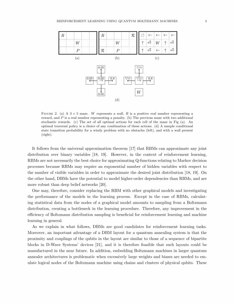
R
W
P
(a)
R
W
R
R
P
(b)
W
↑
←
←↑←←↑←↑
← ←↑↑←↑←↑
(c)
→
0.05
0.05
0.80.05 0.05 →
W
1/15
1/15 0.81/15
(d)
Figure 2. (a) A 3 × 5 maze. W represents a wall, R is a positive real number representing areward, and P is a real number representing a penalty. (b) The previous maze with two additionalstochastic rewards. (c) The set of all optimal actions for each cell of the maze in Fig (a). Anoptimal traversal policy is a choice of any combination of these actions. (d) A sample conditionalstate transition probability for a windy problem with no obstacles (left), and with a wall present(right).
It follows from the universal approximation theorem [17] that RBMs can approximate any joint
distribution over binary variables [18, 19]. However, in the context of reinforcement learning,
RBMs are not necessarily the best choice for approximating Q-functions relating to Markov decision
processes because RBMs may require an exponential number of hidden variables with respect to
the number of visible variables in order to approximate the desired joint distribution [18, 19]. On
the other hand, DBMs have the potential to model higher-order dependencies than RBMs, and are
more robust than deep belief networks [20].
One may, therefore, consider replacing the RBM with other graphical models and investigating
the performance of the models in the learning process. Except in the case of RBMs, calculat-
ing statistical data from the nodes of a graphical model amounts to sampling from a Boltzmann
distribution, creating a bottleneck in the learning procedure. Therefore, any improvement in the
efficiency of Boltzmann distribution sampling is beneficial for reinforcement learning and machine
learning in general.
As we explain in what follows, DBMs are good candidates for reinforcement learning tasks.
Moreover, an important advantage of a DBM layout for a quantum annealing system is that the
proximity and couplings of the qubits in the layout are similar to those of a sequence of bipartite
blocks in D-Wave Systems’ devices [21], and it is therefore feasible that such layouts could be
manufactured in the near future. In addition, embedding Boltzmann machines in larger quantum
annealer architectures is problematic when excessively large weights and biases are needed to em-
ulate logical nodes of the Boltzmann machine using chains and clusters of physical qubits. These

4 D. CRAWFORD, A. LEVIT, N.GHADERMARZY, J. S. OBEROI, AND P. RONAGH
are the reasons why, instead of attempting to embed a Boltzmann machine structure on an existing
quantum annealing system as in [22, 23, 24, 25], we work under the assumption that the network
itself is the native connectivity graph of a near-future quantum annealer, and, using numerical
simulations, we attempt to understand its applicability to reinforcement learning.
We also refer the reader to current trends in machine learning using quantum circuits, specifically,
[26] and [27] for reinforcement learning, and [28] and [29] for training quantum Boltzmann machines
with applications in deep learning and tomography. To the best of our knowledge, the present paper
complements the literature on quantum machine learning as the first proposal on reinforcement
learning using adiabatic quantum computation.
Quantum Monte Carlo (QMC) numerical simulations have been found to be useful in simulat-
ing time-dependant quantum systems. Simulated quantum annealing (SQA) [30, 31], one of the
many flavours of QMC methods, is based on the Suzuki–Trotter expansion of the path integral
representation of the Hamiltonian of Ising spin models in the presence of a transverse field driver
Hamiltonian. Even though the efficiency of SQA for finding the ground state of an Ising model is
topologically obstructed [32], we consider the samples generated by SQA to be good approxima-
tions of the Boltzmann distribution of the quantum Hamiltonian [33]. Experimental studies have
shown similarities in the behaviour of SQA and that of quantum annealing [34, 35] and its physical
realization by D-Wave Systems [36, 37].
We expect that when SQA is set such that the final strength of the transverse field is negligible,
the distribution of the samples approaches the classical limit one expects to observe in absence
of the transverse field. Another classical algorithm which can be used to obtain samples from
the Boltzmann distribution is conventional simulated annealing (SA), which is based on thermal
annealing. Note that this algorithm can be used to create Boltzmann distributions from the Ising
spin model only in the absence of a transverse field. It should, therefore, be possible to use SA or
SQA to approximate the Boltzmann distribution of a classical Boltzmann machine. However, unlike
in the case of SA, it is possible to use SQA not only to approximate the Boltzmann distribution
of a classical Boltzmann machine, but also that of a graphical model in which the energy operator
is a quantum Hamiltonian in the presence of a transverse field. These graphical models, called
quantum Boltzmann machines (QBM), were first introduced in [38].
We use SQA simulations to provide evidence that a quantum annealing device that approximates
the distribution of a DBM or a QBM may improve the learning process compared to a reinforcement
learning method that uses classical RBM techniques. Other studies have shown that SQA is more
efficient than thermal SA [30, 31]. Therefore, our method, used in conjunction with SQA, can also
be viewed as a quantum-inspired approach for reinforcement learning.
What distinguishes our work from current trends in quantum machine learning is that (i) we
consider the use of quantum annealing in reinforcement learning applications rather than frequently
studied classification or recognition problems; (ii) using SQA-based numerical simulations, we as-
sume that the connectivity graph of a DBM directly maps to the native layout of a feasible quantum

REINFORCEMENT LEARNING USING QUANTUM BOLTZMANN MACHINES 5
annealer; and (iii) the results of our experiments using SQA to simulate the sampling of an entan-
gled system of spins suggest that using quantum annealers in reinforcement learning tasks can offer
an advantage over thermal sampling.
2. Preliminaries
2.1. Adiabatic Evolution of Open Quantum Systems. The evolution of a quantum system
under a slowly changing time-dependent Hamiltonian is characterized by the quantum adiabatic
theorem (QAT). QAT has a long history going back to the work of Born and Fock [39]. Colloquially,
QAT states that a system remains close to its instantaneous steady state provided there is a gap
between the eigenenergy of the steady state and the rest of the Hamiltonian’s spectrum at every
point in time if the evolution is sufficiently slow. This result motivated [40] and [41] to introduce the
closely related paradigms of quantum computing known as quantum annealing (QA) and adiabatic
quantum computation (AQC).
QA and AQC, in turn, inspired efforts in the manufacturing of physical realizations of adia-
batic evolution via quantum hardware ([6]). In reality, the manufactured chips operate at nonzero
temperature and are not isolated from their environment. Therefore, the existing adiabatic theory
did not describe the behaviour of these machines. A contemporary investigation in quantum adi-
abatic theory was thus initiated to study adiabaticity in open quantum systems ([1, 2, 3, 4, 5]).
These references prove adiabatic theorems to various degrees of generality and under a variety of
assumptions about the system.
In fact, [2] develops an adiabatic theory for equations of the form
(1) εx(s) = L(s)x(s),
where L is a family of linear operators on a Banach space and L(s) is a generator of a contrac-
tion semigroup for every s. This provides a general framework that encompasses many adiabatic
theorems, including that of classical stochastic systems, all the way to quantum evolutions of open
systems generated by Lindbladians. The manifold of instantaneous stationary states is identical
to ker(L(s)), and [2] shows that the dynamics of the system are parallel-transported along this
manifold as ε→ 0.
An example of (1) is the case in which the Banach space is the space of bounded operators on a
Hilbert space, and in this case we study the evolution of the density matrix ρ of a quantum system.
The Lindbladian is defined via the adjoint action of a Hermitian H on ρ, and couplings to the heat
bath are represented via a family of operators Γα with∑
α Γ∗αΓα being bounded:
Lρ = −i[H, ρ] +1
2
∑α
([Γαρ,Γ∗α] + [Γα, ρΓ∗α]).
In the work of [2], it was then proven that ρ(s) is parallel-transported along ker(L(s)), and that if
L:
(i) is the generator of a contraction semigroup;
(ii) has closed and complementary range and kernel;

6 D. CRAWFORD, A. LEVIT, N.GHADERMARZY, J. S. OBEROI, AND P. RONAGH
(iii) is Ck with respect to s; and
(iv) is constant near the endpoints s = 0 and s = 1;
then the solution to (1) with initial condition in ker(L(0)) deviates only in O(εk) from ker(L(1))
at s = 1.
The authors of [5] focuses on estimating the adiabatic error in terms of the physical parameters
of the theory. In particular, they study the case of a quantum system coupled to a thermal bath
satisfying the Kubo–Martin–Schwinger (KMS) condition. Given a distance δ, in order for the norm
of the solution of (1) to stay δ-close to the instantaneous steady state of the system at s = 1, they
show that ε has to decrease at a rate of O(λ2), where λ denotes the smallest nonzero eigenvalue in
L. Note that the KMS condition implies that the Gibbs state exp(−βH(s))/ tr[exp(−βH(s))] is,
in fact, in ker(L(s)).
This stream of research suggests promising opportunities to use quantum annealers to sample
from the Gibbs state of a quantum Hamiltonian using adiabatic evolution. In this paper, the
transverse field Ising model (TFIM) has been the centre of attention. In practice, due to additional
complications in quantum annealing (e.g., level crossings and gap closure), the samples gathered
from the quantum annealer are far from the Gibbs state of the final Hamiltonian. In fact, [42]
suggests that the distribution of the samples would correspond more closely to an instantaneous
Hamiltonian at an intermediate point in time, called the freeze-out point. Therefore, our goal is
to investigate the applicability of sampling from a TFIM with significant Γ to free energy–based
reinforcement learning.
2.2. Simulated Quantum Annealing. Simulated quantum annealing (SQA) methods are a class
of quantum-inspired algorithms that perform discrete optimization by classically simulating quan-
tum tunnelling phenomena (see [43, p. 422] for an introduction). The algorithm used in this paper
is a single spin-flip version of quantum Monte Carlo numerical simulation based on the Suzuki–
Trotter formula, and uses the Metropolis acceptance probabilities. The SQA algorithm simulates
the quantum annealing phenomena of an Ising spin model with a transverse field, that is,
(2) H(t) = −∑i,j
Jijσzi σ
zj −
∑i
hiσzi − Γ(t)
∑i
σxi ,
where σz and σx represent the Pauli z- and x-matrices, respectively, the indices i and j range over
the sites of the system, and the time t ranges from 0 to 1. In this quantum evolution, the strength
of the transverse field is slowly reduced to zero at finite temperature. In our implementations, we
have used a linear transverse field schedule for the SQA algorithm as in [31] and [44]. Based on the
Suzuki–Trotter formula, the key idea of this algorithm is to approximate the partition function of
the Ising model with a transverse field as a partition function of a classical Hamiltonian denoted
by Heff , corresponding to a classical Ising model of one dimension higher. More precisely,
(3) Heff(σ) = −∑i,j
r∑k=1
Jijrσikσjk − J+
∑i
r∑k=1
σikσi,k+1 −∑i
r∑k=1
hirσik ,

REINFORCEMENT LEARNING USING QUANTUM BOLTZMANN MACHINES 7
where r is the number of replicas, J+ = 12β log coth
(Γβr
), and σik represent spins of the classical
system of one dimension higher.
In our experiments, the strength Γ of the transverse field is scheduled to linearly decrease from
20.00 to one of Γf = 0.01 or 2.00. The inverse temperature β is set to the constant 2.00. The initial
value, 20.00, of the transverse field is empirically chosen to be well above the coupling strengths
created during the training. Each spin is replicated 25 times to represent the Trotter slices in the
extra dimension. The simulation is set to iterate over all replications of all spins one time per
sweep, and the number of sweeps is set to 300, which appears to be large enough for the sizes of
Ising models constructed during our experiments. For each instance of input, the SQA algorithm
is run 150 times. After termination, the configuration of each replica, as well as the configuration
of the entire classical Ising model of one dimension higher, is returned.
Although the SQA algorithm does not follow the dynamics of a physical quantum annealer explic-
itly, it is used to simulate this process, as it captures major quantum phenomena such as tunnelling
and entanglement [34]. In [34], for example, it is shown that quantum Monte Carlo simulations can
be used to understand the tunnelling behaviour in quantum annealers. As mentioned previously,
it readily follows from the results of [33] that the limiting distribution of SQA is the Boltzmann
distribution of Heff . This makes SQA a candidate classical algorithm for sampling from Boltzmann
distributions of classical and quantum Hamiltonians. The former is achieved by setting Γf ' 0,
and the latter by constructing an effective Hamiltonian of the system of one dimension higher, rep-
resenting the quantum Hamiltonian with non-negligible Γf . Alternatively, a classical Monte Carlo
simulation used to sample from the Boltzmann distribution of the classical Ising Hamiltonian is the
SA algorithm, based on thermal fluctuations of classical spin systems.
2.3. Markov Decision Process. The stochastic control problem of interest to us is a Markov
decision process (MDP), defined as having:
(i) finite sets of states S and actions A;
(ii) a controlled Markov chain [45], defined by a transition kernel P(s′ ∈ S|s ∈ S, a ∈ A);
(iii) a real-valued function r : S ×A→ R, known as the immediate reward structure; and
(iv) a constant γ ∈ [0, 1), known as the discount factor.
A function π : S → A is called a stationary policy ; that is, it is a choice of action π(s) for every
state s independent of the point in time that the controlled process reaches s. The application of a
stationary policy π reduces the MDP into a time-homogeneous Markov chain Π, with a transition
probability P(s′|s, π(s)). The random process Π with initial condition Π0 = s we denote by Πs.
Our Markov decision problem is to find
π∗(s) = argmaxπ
V (π, s),(4)
When both S and A are finite, the MDP is said to be finite.The transition kernel does not need to be time-homogeneous; however, this definition suffices for the purposes of
this work.For more-general statements, see [45].
8 D. CRAWFORD, A. LEVIT, N.GHADERMARZY, J. S. OBEROI, AND P. RONAGH
where
V (π, s) = E
[ ∞∑i=0
γi r(Πsi , π(Πs
i ))
].(5)
2.3.1. Maze Traversal as a Markov Decision Process. Maze traversal is a problem typically used
to develop and benchmark reinforcement learning algorithms [46]. A maze is structured as a two-
dimensional grid of r rows and c columns in which a decision-making agent is free to move up,
down, left, or right, or to stand still. During the maze traversal, the agent encounters obstacles
(e.g., walls), rewards (e.g., goals), and penalties (negative rewards, e.g., a pit). Each cell of the
maze can contain either a deterministic or stochastic reward, a wall, a pit, or a neutral value.
Fig. 2a and Fig. 2b show examples of two mazes. Fig. 2c shows the corresponding solutions to the
maze in Fig. 2a.
The goal of the reinforcement learning algorithm in the maze traversal problem is for the agent
to learn the optimal action to take in each cell of the maze by maximizing the total reward, that is,
finding a route across the maze that avoids walls and pits while favouring rewards. This problem
can be modelled as an MDP determined by the following components:
• The state of the system is the agent’s position within the maze. The position state s takes values
in the set of states
S = {1, ..., r} × {1, ..., c}.• In any state, the agent can decide to take one of the five actions
a ∈ {↑, ↓,←,→,}.
These actions will guide the agent through the maze. An action that would lead the agent into
a wall (W ) or outside of the maze boundary is treated as an inadmissible action. Each action
can be viewed as an endomorphism on the set of states
a : S → S.
If a = , then a(s) = s; otherwise, a(s) is the state adjacent to S in the direction shown by a.
We do not consider training samples where a is inadmissible.
• The transition kernel determines the probability of the agent moving from one state to another
given a particular choice of action. In the simplest case, the probability of transition from s to
a(s) is one:
P(a(s)|s, a) = 1.
We call the maze clear if the associated transition kernel is as above, as opposed to the windy
maze, in which there is a nonzero probability that if the action a is taken at state s, the next
state will differ from a(s).
• The immediate reward r(s, a) that the agent gains from taking an action a in state s is the value
contained in the destination state. Moving into a cell containing a reward returns the favourable

REINFORCEMENT LEARNING USING QUANTUM BOLTZMANN MACHINES 9
value R, moving into a cell containing a penalty returns the unfavourable value P , and moving
into a cell with no reward returns a neutral value in the interval (P,R).
• A discount factor for future rewards is a non-negative constant γ < 1. In our experiments, this
discount factor is set to γ = 0.8. The discount factor is a feature of the problem rather than
a free parameter of an implementation. For example, in a financial application scenario, the
discount factor might be a function of the risk-free interest rate.
The immediate reward for moving into a cell with a stochastic reward is given by a random
variable R. If an agent has prior knowledge of this distribution, then it should be able to treat the
cell as one with a deterministic reward value of E[R]. This allows us to find the set of all optimal
policies in each maze instance. This policy information is denoted by α∗ : S → 2A, associating with
each state s ∈ S a set of optimal actions α∗(s) ⊆ A.
In our maze model, the neutral value is set to 100, the reward R = 200, and the penalty P = 0.
In our experiments, the stochastic reward R is simulated by drawing a sample from the Bernoulli
distribution 200 Ber(0.5); hence, it has the expected value E[R] = 100, which is identical to the
neutral value. Therefore, the solutions depicted in Fig. 2c are solutions to the maze of Fig. 2b as
well.
2.4. Value Iteration. Bellman [47] writes V (π, s) recursively in the following manner using the
monotone convergence theorem:
V (π, s) = E
[ ∞∑i=0
γi r(Πsi , π(Πs
i ))
]
= E[r(Πs0, π(Πs
0))] + γ E
[ ∞∑i=0
γi r(Πsi+1, π(Πs
i+1))
]= E[r(s, π(s))] + γ
∑s′∈S
P(s′|s, π(s))V (π, s′) .
In particular, it leads to the Bellman optimality equation:
(6) V ∗(s) = V (π∗, s) = maxa
(E[r(s, a)] + γ
∑s′∈S
P(s′|s, a)V ∗(s′)
).
Hence, V ∗ is a fixed point for the operator
TV (f) : s 7→ maxa
(E[r(s, a)] + γ
∫f
)on the space L∞(S) of bounded functions S → R endowed with the max norm. Here, the integral
is taken with respect to the probability measure on S, induced by the conditional probability
distribution P(s′|s, a). It is easy to check that TV is a contraction mapping, and thus V ∗ is the
unique fixed point of TV and the uniform limit of any sequence of functions {TnV f}n. Numerical
computation of this limit using (6), called value iteration, is a common method of solving the
Markov decision problem (4). However, even the ε-optimal algorithms for this approach depend

10 D. CRAWFORD, A. LEVIT, N.GHADERMARZY, J. S. OBEROI, AND P. RONAGH
heavily on the cardinality of both S and A, and suffer from the curse of dimensionality [47, 48].
Moreover, the value iteration method requires having full knowledge of the transition probabilities,
as well as the distribution of the immediate rewards.
2.5. Q-functions. For a stationary policy π, the Q-function (also known as the action–value func-
tion) is defined as a mapping of a pair (s, a) to the expected value of the reward of the Markov
chain that begins with taking action a at initial state s and continuing according to π [8]:
Q(π, s, a) = E[r(s, a)] + E
[ ∞∑i=1
γi r(Πsi , π(Πs
i ))
].
It is straightforward to check that
V (π∗, s) = maxa
Q(π∗, s, a),
and for Q∗(s, a) = maxπ Q(π, s, a) = Q(π∗, s, a), the optimal policy for the MDP can be retrieved
via the following:
π∗(s) = argmaxa
Q∗(s, a).(7)
This reduces the Markov decision problem to computing Q∗(s, a). The Bellman optimality equation
for Q∗(s, a) is
Q∗(s, a) = E[r(s, a)] + γ∑s′
P(s′|s, a) maxa′
Q∗(s′, a′),
which makes Q∗ the fixed point of a different operator
TQ(f) : (s, a) 7→ E[r(s, a)] + γ
∫maxa′
f
defined on L∞(S ×A).
2.6. Temporal-Difference Gradient Descent. In this section, we derive the Q-learning method
for MDPs. From the previous section, we know that starting from an initial Q0 : S × A → R, the
sequence {Qn = TnQQ0} converges to Q∗. The difference
(8) Qn+1(s, a)−Qn(s, a) = E[r(s, a)] + γ∑s′
P(s′|s, a) maxa
Qn(s′, a)︸ ︷︷ ︸(∗)
−Qn(s, a)
is called the temporal difference of Q-functions, and is denoted by ETD.
Employing a gradient approach to find the fixed point of T on L∞(S × A) involves locally
parametrizing the functions in this space by a vector of parameters θ, that is,
Q(s, a) = Q(s, a;θ),
and travelling in the direction that minimizes ‖ETD‖2:
∆θ ∝ −ETD∇θETD .(9)
REINFORCEMENT LEARNING USING QUANTUM BOLTZMANN MACHINES 11
The method TD(0) consists of treating the (∗) in (8) as constant with respect to the parameter-
ization θ, in which case we may write
∆θ ∝∼ ETD(s, a)∇θQ(s, a;θ).
For an agent agnostic with respect to the transition kernel or the distribution of the reward
r(s, a), or both, this update rule for θ is not possible. The alternative is to substitute, at each
iteration, the expected value ∑s′
P(s′|s, a) maxa
Qn(sn+1, a)
by maxaQn(sn+1, a), where sn+1 is drawn from the probability distribution P(s′|s, a), and substitute
E[r(sn, an)] by a sample of r(sn, an). This leads to a successful Monte Carlo training method called
Q-learning .
In what follows, we explain the case in which θ comprises the weights of a Boltzmann machine.
Let us begin by introducing clamped Boltzmann machines, which are of particular importance in
the case of reinforcement learning.
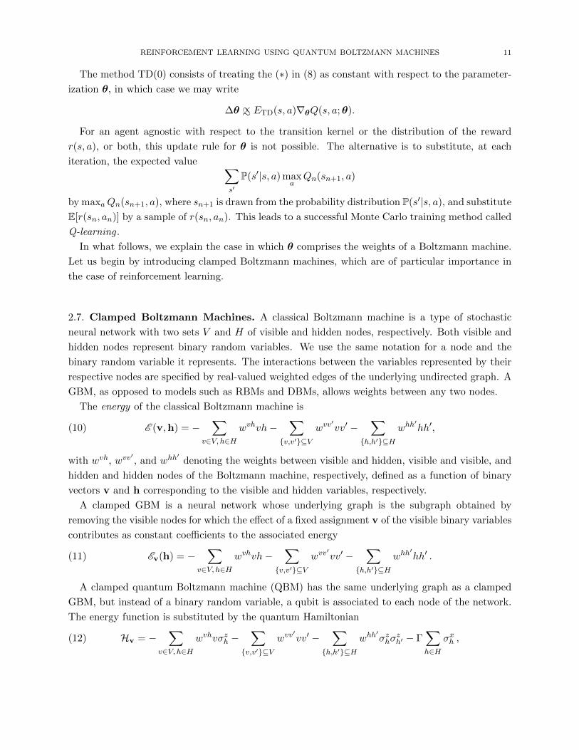
2.7. Clamped Boltzmann Machines. A classical Boltzmann machine is a type of stochastic
neural network with two sets V and H of visible and hidden nodes, respectively. Both visible and
hidden nodes represent binary random variables. We use the same notation for a node and the
binary random variable it represents. The interactions between the variables represented by their
respective nodes are specified by real-valued weighted edges of the underlying undirected graph. A
GBM, as opposed to models such as RBMs and DBMs, allows weights between any two nodes.
The energy of the classical Boltzmann machine is
(10) E (v,h) = −∑
v∈V, h∈Hwvhvh−
∑{v,v′}⊆V
wvv′vv′ −
∑{h,h′}⊆H
whh′hh′,
with wvh, wvv′, and whh
′denoting the weights between visible and hidden, visible and visible, and
hidden and hidden nodes of the Boltzmann machine, respectively, defined as a function of binary
vectors v and h corresponding to the visible and hidden variables, respectively.
A clamped GBM is a neural network whose underlying graph is the subgraph obtained by
removing the visible nodes for which the effect of a fixed assignment v of the visible binary variables
contributes as constant coefficients to the associated energy
(11) Ev(h) = −∑
v∈V, h∈Hwvhvh−
∑{v,v′}⊆V
wvv′vv′ −
∑{h,h′}⊆H
whh′hh′ .
A clamped quantum Boltzmann machine (QBM) has the same underlying graph as a clamped
GBM, but instead of a binary random variable, a qubit is associated to each node of the network.
The energy function is substituted by the quantum Hamiltonian
(12) Hv = −∑
v∈V, h∈Hwvhvσzh −
∑{v,v′}⊆V
wvv′vv′ −
∑{h,h′}⊆H
whh′σzhσ
zh′ − Γ
∑h∈H
σxh ,

12 D. CRAWFORD, A. LEVIT, N.GHADERMARZY, J. S. OBEROI, AND P. RONAGH
where σzh represent the Pauli z-matrices and σxh represent the Pauli x-matrices. Thus, a clamped
QBM with Γ = 0 is equivalent to a clamped classical Boltzmann machine. This is because Hv
is a diagonal matrix in the σz-basis, the spectrum of which is identical to the range of Ev. The
remainder of this section is formulated for the clamped QBMs, acknowledging that it can easily be
specialized to clamped classical Boltzmann machines.
Let β = 1kBT
be a fixed thermodynamic beta. For an assignment of visible variables v, F (v)
denotes the equilibrium free energy, and is defined as
F (v) := − 1
βlnZv = 〈Hv〉+
1
βtr(ρv ln ρv) .(13)
Here, Zv = tr(e−βHv) is the partition function of the clamped QBM and ρv is the density matrix
ρv = 1Zve−βHv . The term − tr(ρv ln ρv) is the entropy of the system. The notation 〈· · · 〉 is used
for the expected value of any observable with respect to the Gibbs measure, in particular,
〈Hv〉 =1
Zvtr(Hve
−βHv).
2.8. Reinforcement Learning Using Clamped Boltzmann Machines. In this section, we
explain how a general Boltzmann machine (GBM) can be used to provide a Q-function approximator
in a Q-learning method. To the best of our knowledge, this derivation has not been previously given,
although it can be readily derived from the ideas presented in [16] and [38]. Following [16], the goal
is to use the negative free energy of a Boltzmann machine to approximate the Q-function through
the relationship
Q(s, a) ≈ −F (s,a) = −F (s,a;θ)
for each admissible state–action pair (s, a) ∈ S ×A. Here, s and a are binary vectors encoding the
state s and action a on the state nodes and action nodes, respectively, of the Boltzmann machine.
In reinforcement learning, the visible nodes of the GBM are partitioned into two subsets of state
nodes S and action nodes A.
The parameters θ, to be trained according to a TD(0) update rule (see Sec. 2.6), are the weights
in a Boltzmann machine. For every weight w, the update rule is
∆w = −ε(rn(sn, an) + γmaxa
Q(sn+1, a)−Q(sn, an))∂F
∂w.
From (13), we obtain
∂F (s,a)
∂w= − 1
βZs,a
∂
∂wtr(e−βHs,a
)=
1
βZs,atr
(βe−βHs,a
∂
∂wHs,a
)=
⟨∂
∂wHs,a
⟩.
Therefore, the update rule for TD(0) for the clamped QBM can be rewritten as
(14) ∆wvh = ε(rn(sn, an) + γQ(sn+1, an+1)−Q(sn, an))v〈σzh〉

REINFORCEMENT LEARNING USING QUANTUM BOLTZMANN MACHINES 13
and
(15) ∆whh′
= ε(rn(sn, an) + γQ(sn+1, an+1)−Q(sn, an))〈σzhσzh′〉,
where the thermodynamic beta is absorbed into the learning rate ε, and
an+1 = argmaxa
Q(sn+1, a).
Here, h and h′ denote two distinct hidden nodes and (by a slight abuse of notation) the letter v
stands for a visible (state or action) node, and also the value of the variable associated to that
node.
To approximate the right-hand side of each of (14) and (15), we use SQA experiments. By [49,
Theorem 6], we may find the expected values of the observables 〈σzh〉 and 〈σzhσzh′〉 by averaging
the corresponding spins in the classical Ising model of one dimension higher used in SQA. To
approximate the Q-function, we take advantage of [49, Theorem 4] and use (13) applied to this
classical Ising model. More precisely, let Heffv represent the Hamiltonian of the classical Ising model
of one dimension higher and the associated energy function E effv . The free energy of this model can
be written
F (v) = 〈Heffv 〉+
1
β
∑c
P(c|v) logP(c|v) ,(16)
where c ranges over all spin configurations of the classical Ising model of one dimension higher.
The above argument holds in the absence of the transverse field, that is, for the classical Boltz-
mann machine. In this case, the TD(0) update rule is given by
(17) ∆wvh = ε(rn(sn, an) + γQ(sn+1, an+1)−Q(sn, an))v〈h〉
and
(18) ∆whh′
= ε(rn(sn, an) + γQ(sn+1, an+1)−Q(sn, an))〈hh′〉 ,
where 〈h〉 (referred to as activations of the hidden nodes in machine learning terminology) and
〈hh′〉 are the expected values of the variables and the product of variables, respectively, in the
binary encoding of the hidden nodes with respect to the Boltzmann distribution given by P(h|v) =
exp(−βEv(h))/∑
h′ exp(−βEv(h′)). Therefore, they may be approximated using SA or SQA when
Γ→ 0.
The values of the Q-functions in (17) and (18) can also be approximated empirically, since, in a
classical Boltzmann machine,
F (v) =∑h
P(h|v)Ev(h) +1
β
∑h
P(h|v) logP(h|v)(19)
= −∑s∈Sh∈H
wshs〈h〉 −∑a∈Ah∈H
waha〈h〉 −∑
{h,h′}⊆H
uhh′〈hh′〉+
1
β
∑h
P(h|s,a) logP(h|s,a).
14 D. CRAWFORD, A. LEVIT, N.GHADERMARZY, J. S. OBEROI, AND P. RONAGH
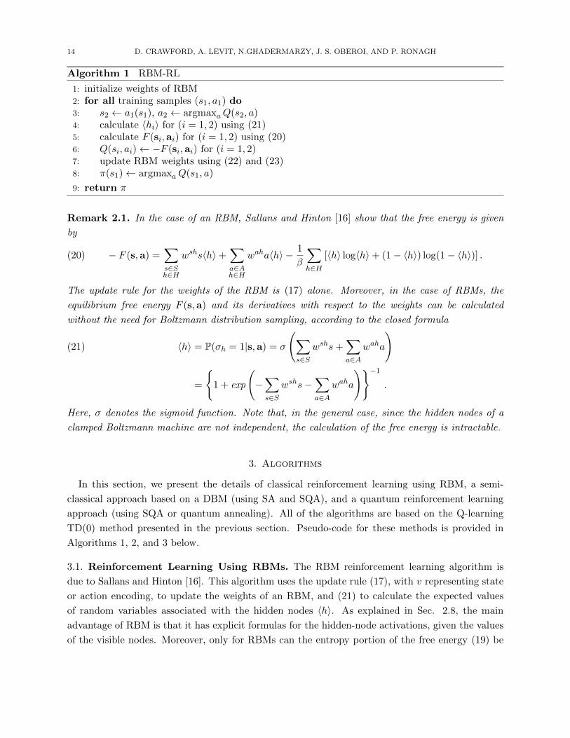
Algorithm 1 RBM-RL
1: initialize weights of RBM2: for all training samples (s1, a1) do3: s2 ← a1(s1), a2 ← argmaxaQ(s2, a)4: calculate 〈hi〉 for (i = 1, 2) using (21)5: calculate F (si,ai) for (i = 1, 2) using (20)6: Q(si, ai)← −F (si,ai) for (i = 1, 2)7: update RBM weights using (22) and (23)8: π(s1)← argmaxaQ(s1, a)
9: return π
Remark 2.1. In the case of an RBM, Sallans and Hinton [16] show that the free energy is given
by
(20) − F (s,a) =∑s∈Sh∈H
wshs〈h〉+∑a∈Ah∈H
waha〈h〉 − 1
β
∑h∈H
[〈h〉 log〈h〉+ (1− 〈h〉) log(1− 〈h〉)] .
The update rule for the weights of the RBM is (17) alone. Moreover, in the case of RBMs, the
equilibrium free energy F (s,a) and its derivatives with respect to the weights can be calculated
without the need for Boltzmann distribution sampling, according to the closed formula
〈h〉 = P(σh = 1|s,a) = σ
(∑s∈S
wshs+∑a∈A
waha
)(21)
=
{1 + exp
(−∑s∈S
wshs−∑a∈A
waha
)}−1
.
Here, σ denotes the sigmoid function. Note that, in the general case, since the hidden nodes of a
clamped Boltzmann machine are not independent, the calculation of the free energy is intractable.
3. Algorithms
In this section, we present the details of classical reinforcement learning using RBM, a semi-
classical approach based on a DBM (using SA and SQA), and a quantum reinforcement learning
approach (using SQA or quantum annealing). All of the algorithms are based on the Q-learning
TD(0) method presented in the previous section. Pseudo-code for these methods is provided in
Algorithms 1, 2, and 3 below.
3.1. Reinforcement Learning Using RBMs. The RBM reinforcement learning algorithm is
due to Sallans and Hinton [16]. This algorithm uses the update rule (17), with v representing state
or action encoding, to update the weights of an RBM, and (21) to calculate the expected values
of random variables associated with the hidden nodes 〈h〉. As explained in Sec. 2.8, the main
advantage of RBM is that it has explicit formulas for the hidden-node activations, given the values
of the visible nodes. Moreover, only for RBMs can the entropy portion of the free energy (19) be

REINFORCEMENT LEARNING USING QUANTUM BOLTZMANN MACHINES 15
Algorithm 2 DBM-RL
1: initialize weights of DBM2: for all training samples (s1, a1) do3: s2 ← a1(s1), a2 ← argmaxaQ(s2, a)4: approximate 〈hi〉, 〈hih′i〉,P(h|si,ai)
using SA or SQA for (i = 1, 2)5: calculate F (si,ai) using (19) for (i = 1, 2)6: Q(si, ai)← −F (si,ai) for (i = 1, 2)7: update DBM weights using (18), (22), and (23)8: π(s1)← argmaxaQ(s1, a)
9: return π
written in terms of the activations of the hidden nodes. More-complicated network architectures
do not possess this property, so there is a need for a Boltzmann distribution sampler.
In Algorithm 1, we recall the steps of the classical reinforcement learning algorithm using an RBM
with a graphical model similar to that shown in Fig. 1a. We set the initial Boltzmann machine
weights using Gaussian zero-mean values with a standard deviation of 1.00, as is common practice
for implementing Boltzmann machines [50]. Consequently, this initializes an approximation of a
Q-function and a policy π given by
π(s) = argmaxa
Q(s, a) .
In each training iteration, we select a state–action pair (s1, a1) ∈ S × A. We associate a classical
spin variable σh to each hidden node h. Then, the activations of the hidden nodes are calculated
via (21). In our experiments, all Boltzmann machines have as many state nodes as |S| and as
many action nodes as |A|. We associate one node for every state s ∈ S, and the corresponding
binary encoding is s = (0, 0, . . . , 1, . . . , 0), with zeroes everywhere except at the index of the node
corresponding to s. We use similar encoding for the actions, using the action nodes. A subsequent
state s2 is obtained from the state–action pair (s1, a1) using the transition kernel outlined in Sec.
2, and a corresponding action a2 is chosen via policy π. The free energy of the RBM is calculated
using (20) for both (s1, a1) and (s2, a2).
This results in an approximation of the Q-function (see Sec. 2.5) defined on the state–action
space S ×A [16],
Q(s, a) ≈ −F (s,a) ,
for both state–action pairs. We then use the update rule (17), or, more precisely,
(22) ∆wsh = ε(r(s1, a1) + γQ(s2, a2)−Q(s1, a1))s1〈h〉
and
(23) ∆wah = ε(r(s1, a1) + γQ(s2, a2)−Q(s1, a1))a1〈h〉 ,
with a learning rate ε to update the weights of the RBM. In view of (7), the best known policy can
be acquired via π(s) = argmaxaQ(s, a) for any state s.

16 D. CRAWFORD, A. LEVIT, N.GHADERMARZY, J. S. OBEROI, AND P. RONAGH
3.2. Reinforcement Learning Using DBMs. Since we are interested in the dependencies be-
tween states and actions, we consider a DBM architecture that has a layer of states connected to
the first layer of hidden nodes, followed by multiple hidden layers, and a layer of actions connected
to the final layer of hidden nodes (see Fig. 1). We demonstrate the advantages of this deep architec-
ture trained using SQA and the derivation in Sec. 2.8 of the temporal-difference gradient method
for reinforcement learning using general Boltzmann machines (GBM).
In Algorithm 2, we summarize the DBM-RL method. Here, the graphical model of the Boltzmann
machine is similar to that shown in Fig. 1b. The initialization of the weights of the DBM is
performed in a similar fashion to the previous algorithm.
In each training iteration, we select a state–action pair (s1, a1) ∈ S×A. Every node corresponding
to a state or an action is removed from the graph and the configurations of the spins corresponding
to the hidden nodes are sampled using SA or SQA on an Ising spin model constructed as follows:
the state s1 contributes to a bias of ws1h to σh if h is adjacent to s1; and the action a1 contributes
to a bias of wa1h to σh if h is adjacent to a1. The bias on any spin σh for which h is a hidden node
not adjacent to state s1 or action a1 is zero.
A subsequent state s2 is obtained from the state–action pair (s1, a1) using the transition kernel
outlined in Sec. 2, and a corresponding action a2 is chosen via policy π. Another SQA sampling is
performed in a similar fashion to the above for this pair.
According to lines 4 and 5 of Algorithm 2, the samples from the SA or SQA algorithm are used
to approximate the free energy of the classical DBM at points (s1, a1) and (s2, a2) using (19).
If SQA is used, averages are taken over each replica of each run; hence, there are 3750 samples
of configurations of the hidden nodes for each state–action pair. The strength Γ of the transverse
field is scheduled to linearly decrease from 20.00 to Γf = 0.01.
The SA algorithm is used with a linear inverse temperature schedule that increases from 0.01 to
2.00 in 50,000 sweeps, and is run 150 times. So, if SA is used, there are only 150 sample points
used in the above approximation. The results of DBM-RL using SA or SQA have no significant
differences.
The final difference between Algorithm 1 and Algorithm 2 is that the update rule now includes
updates of weights between two hidden nodes given by (18),
(24) ∆whh′
= ε(r(s1, a1) + γQ(s2, a2)−Q(s1, a1))〈hh′〉 ,
in addition to the previous rules (22) and (23).
3.3. Reinforcement Learning Using QBMs. The last algorithm is QBM-RL, presented in
Algorithm 3. The initialization is performed as in Algorithms 1 and 2. However, according to lines
4 and 5, the samples from the SQA algorithm are used to approximate the free energy of a QBM
at points (s1, a1) and (s2, a2) by computing the free energy corresponding to an effective classical
Ising spin model of one dimension higher representing the quantum Ising spin model of the QBM,
via (16).

REINFORCEMENT LEARNING USING QUANTUM BOLTZMANN MACHINES 17
In this case, 〈Heffs,a〉 from (16) is approximated by the average energy of the entire system of one
dimension higher and P(c|s,a) is approximated by the normalized frequency of the configuration
c of the entire system of one dimension higher (hence, there are only 150 sample points for each
input instance in this case). The strength Γ of the transverse field in SQA is scheduled to linearly
decrease from 20.00 to Γf = 2.00. In this algorithm, the weights are updated as in Algorithm 2.
However, 〈h〉 and 〈hh′〉 in this algorithm represent expectations of measurements in the z-basis.
In each training iteration, we select a state–action pair (s1, a1) ∈ S×A. Every node corresponding
to a state or an action is removed from this graph and the configurations of the spins corresponding
to the hidden nodes are sampled using SQA on an Ising spin model constructed as follows: the
state s1 contributes to a bias of ws1h to σh if h is adjacent to s1; and the action a1 contributes to
a bias of wa1h to σh if h is adjacent to a1. The bias on any spin σh for which h is a hidden node
not adjacent to state s1 or action a1 is zero.
A subsequent state s2 is obtained from the state–action pair (s1, a1) using the transition kernel
outlined in Sec. 2, and a corresponding action a2 is chosen via policy π. Another SQA sampling is
performed in a similar fashion to the above for this pair.
In Fig. 3a and Fig. 3b, the selection of (s1, a1) is performed by sweeping across the set of state–
action pairs. In Fig. 3d, the selection of (s1, a1) and s2 is performed by sweeping over S × A× S.
In Fig. 3c, the selection of s1, a1, and s2 are all performed uniformly randomly.
We experiment with a variety of learning-rate schedules, including exponential, harmonic, and
linear; however, we found that for the training of both RBMs and DBMs, an adaptive learning-
rate schedule performed best (for information on adaptive subgradient methods, see [51]). In our
experiments, the initial learning rate is set to 0.01.
In all of our studied algorithms, training terminates when a desired number of training samples
have been processed, after which the updated policy is returned.
4. Numerical Results
We study the performance of temporal-difference reinforcement learning algorithms (explained
in detail in Sec. 3) using Boltzmann machines. We generalize the method introduced in [16], and
Algorithm 3 QBM-RL
1: initialize weights of QBM2: for all training samples (s1, a1) do3: s2 ← a1(s1), a2 ← argmaxaQ(s2, a)4: approximate 〈hi〉, 〈hih′i〉, 〈Heff
si,ai〉,
and P(c|si,ai) using SQA for (i = 1, 2)5: calculate F (si,ai) using (16) for (i = 1, 2)6: Q(si, ai)← −F (si,ai) for (i = 1, 2)7: update QBM weights using (18), (22), and (23)8: π(s1)← argmaxaQ(s1, a)
9: return π

18 D. CRAWFORD, A. LEVIT, N.GHADERMARZY, J. S. OBEROI, AND P. RONAGH
compare the policies obtained from these algorithms to the optimal policy using a fidelity measure,
which we define in (25).
For Tr independent trials of the same reinforcement learning algorithm, Ts training samples are
used for reinforcement learning. The fidelity measure at the i-th training sample is defined by
(25) fid(i) = (Tr × |S|)−1Tr∑l=1
∑s∈S
1A(s,i,l)∈α∗(s),
where A(s, i, l) denotes the action assigned at the l-th run and i-th training sample to the state s.
In our experiments, each algorithm is run 1440 times, and for each run of an algorithm, Ts = 500
training samples are generated.
Fig. 3a and Fig. 3b show the fidelity of the generated policies obtained from various reinforcement
learning experiments on two clear 3× 5 mazes. In Fig. 3a, the maze includes one reward, one wall,
and one pit, and in Fig. 3b, the maze additionally includes two stochastic rewards. In these
experiments, the training samples are generated by sweeping over the maze. Each sweep iterates
over the maze elements in the same order. This explains the periodic behaviour of the fidelity
curves (cf. Fig. 3c).
The curves labelled ‘QBM-RL’ represent the fidelity of reinforcement learning using QBMs.
Sampling from the QBM is performed using SQA. All other experiments use classical Boltzmann
machines as their graphical model. In the experiment labelled ‘RBM-RL’, the graphical model
is an RBM, trained classically using formula (21). The remaining curve is labelled ‘DBM-RL’ for
classical reinforcement learning using a DBM. In these experiments, sampling from configurations of
the DBM is performed with SQA (with Γf = 0.01). The fidelity results of DBM-RL coincide closely
with those of sampling configurations of the DBM using SA; therefore, we have not included them.
Fig. 3c regenerates the results of Fig. 3a using uniform random sampling (i.e., without sweeping
through the maze).
Our next result, shown in Fig. 3d, compares RBM-RL, DBM-RL, and QBM-RL for a windy
maze of size 3× 5. The transition kernel for this experiment is chosen such that P(a(s)|s, a) = 0.8,
and P(s′|s, a) has a nonzero value for all s′ 6= a(s) that are reachable from s by taking some action,
in which case all these values are equal. The transition probability is zero for all other states.
Fig. 2d shows examples of the transition probabilities in the windy problem.
To demonstrate the performance of RBM-RL, DBM-RL, and QBM-RL with respect to scaling,
we define another measure called average fidelity, av`, where we take the average fidelity over the
last ` training samples of the fidelity measure. Given Ts total training samples and fid(i) as defined
above, we write
av` =1
`
Ts∑i=Ts−`
fid(i) .
In Fig. 4, we report the effect of maze size on av` for RBM-RL, DBM-RL, and QBM-RL for varying
maze sizes. We plot av` for each algorithm with ` = 500, 250, and 10 as a function of maze size

REINFORCEMENT LEARNING USING QUANTUM BOLTZMANN MACHINES 19
0 100 200 300 400 500
Training Sample
0.0
0.2
0.4
0.6
0.8
1.0
fid1R1W1P
(a)
0 100 200 300 400 500
Training Sample
0.0
0.2
0.4
0.6
0.8
1.0
fid
3R1W1P
(b)
0 100 200 300 400 500
Training Sample
0.0
0.2
0.4
0.6
0.8
1.0
fid
1R1W1P
(c)
0 100 200 300 400 500
Training Sample
0.0
0.2
0.4
0.6
0.8
1.0
fid
1R1W1P-windy
(d)
RBM-RL DBM-RL QBM-RL
Figure 3. Comparison of RBM-RL, DBM-RL, and QBM-RL training results. Every underlyingRBM has 16 hidden nodes and every DBM has two layers of eight hidden nodes. The shaded areasindicate the standard deviation of each training algorithm. (a) The fidelity curves for the threealgorithms run on the maze in Fig 2a. (b) The fidelity curves for the maze in Fig 2b. (c) Thefidelity curves of the mentioned three algorithms corresponding to the same experiment as thatof (a), except that the training is performed by uniformly generated training samples rather thansweeping across the maze. (d) The fidelity curves corresponding to a windy maze similar to Fig 2a.
for a family of problems with one deterministic reward, two stochastic rewards, one pit, and n− 2
walls. We use nine n× 5 mazes in this experiment, indexed by various values of n. In addition to
the av` plots, we include a dotted-line plot depicting the fidelity for a completely random policy.
The fidelity of the random policy is given by the average probability of choosing an optimal action
at each state when generating admissible actions uniformly at random, which is given by 18n+748n+24 .
Note that the fidelity of the random policy increases as the maze size increases. This is due to the

20 D. CRAWFORD, A. LEVIT, N.GHADERMARZY, J. S. OBEROI, AND P. RONAGH
R RW
W
W
...
R
P
W
W
...
↑
←
←
↑ ←↑ ↑ ←↑
↑ ←↑←↑
↑↑←↑←↑
← ← ←
n−
2
5
(a)
2×
5
3×
5
4×
5
5×
5
6×
5
7×
5
8×
5
9×
5
10×
5
Maze Size
0.0
0.2
0.4
0.6
0.8
1.0
av`
3R(n−2)W1P - QBM/DBM [10,10], RBM [20]
DBM-RL, `= 500
DBM-RL, `= 250
DBM-RL, `= 10
RBM-RL, `= 500
RBM-RL, `= 250
RBM-RL, `= 10
QBM-RL, `= 500
QBM-RL, `= 250
QBM-RL, `= 10
(b)
Figure 4. A comparison between the performance of RBM-RL, DBM-RL, and QBM-RL as thesize of the maze grows. All Boltzmann machines have 20 hidden nodes. (a) The schematics of ann× 5 maze with one deterministic reward, 2 stochastic rewards, one pit, and n− 2 walls. (b) Thescaling of the average fidelity of each algorithm run on each instance of the n×5 maze. The dottedline is the average fidelity of uniformly randomly generated actions.
fact that maze rows containing a wall have more average admissible optimal actions than the top
and bottom rows of the maze.
5. Discussion
The fidelity curves in Fig. 3 show that DBM-RL outperforms RBM-RL with respect to the
number of training samples. Therefore, we expect that in conjunction with a high-performance
sampler of Boltzmann distributions (e.g., a quantum or a quantum-inspired oracle taken as such),
DBM-RL improves the performance of reinforcement learning. QBM-RL is not only on par with
DBM-RL, but actually slightly improves upon it by taking advantage of sampling in the presence
of a significant transverse field.
This is a positive result for the potential of sampling from a quantum device in machine learn-
ing, as we do not expect quantum annealing to obtain the Boltzmann distribution of a classical
Hamiltonian [42, 52, 53]. However, given the discussion in Sec. 2.1, a quantum annealer viewed

REINFORCEMENT LEARNING USING QUANTUM BOLTZMANN MACHINES 21
as an open system coupled to a heat bath could be a better choice of sampler from its instanta-
neous Hamiltonian in earlier stages of the annealing process, compared to a sampler of the problem
Hamiltonian at the end of the evolution. Therefore, these experiments address whether a quantum
Boltzmann machine with a transverse field Ising Hamiltonian can perform at least as well as a
classical Boltzmann machine.
In each experiment, the fidelity curves from DBM-RL produced using SQA with Γf = 0.01 match
the ones produced using SA. This is consistent with our expectation that using SQA with Γ → 0
produces samples from the same distribution as SA, namely, the Boltzmann distribution of the
classical Ising Hamiltonian with no transverse field.
The best algorithm in our experiments is evidently QBM-RL using SQA. Here, the final trans-
verse field is Γf = 2.00, corresponding to one-third of the anneal for a quantum annealing algorithm
that evolves along the convex linear combination of the initial and final Hamiltonians with constant
speed. This is consistent with ideas found in [38] on sampling at freeze-out [42].
Fig. 3c shows that, whereas the maze can be solved with fewer training samples using ordered
sweeps of the maze, the periodic behaviour of the fidelity curves is due to this periodic choice of
training samples. This effect disappears once the training samples are chosen uniformly randomly.
Fig. 3d shows that the improvement in the learning of the DBM-RL and QBM-RL algorithms
persists in the case of more-complicated transition kernels. The same ordering of fidelity curves
discussed earlier is observed: QBM-RL outperforms DBM-RL, and DBM-RL outperforms RBM-
RL.
It is worth mentioning that, even though it may seem that more connectivity between the
hidden nodes may allow a Boltzmann machine to capture more- complicated correlations between
the visible nodes, the training process of the Boltzmann machine becomes more computationally
involved. In our reinforcement learning application, an RBM with m hidden nodes, and n = |S|+|A|visible nodes, has mn weights to train. A DBM with two hidden layers of equal size has 1
4m(2n+m)
weights to train. Therefore, when m < 2n, the training of the DBM is in a domain of a lower
dimension. Further, a GBM with all of its hidden nodes forming a complete graph requires mn+(m2
)weights to train, which is always larger than that of an RBM or a DBM with the same number of
hidden nodes.
One can observe from Fig. 4 that, as the maze size increases and the complexity of the rein-
forcement learning task increases, av` decreases for each algorithm. The RBM algorithm, while
always outperformed by DBM-RL and QBM-RL, shows a much faster decay in average fidelity as
a function of maze size compared to both DBM-RL and QBM-RL. For larger mazes, the RBM
algorithm fails to capture maze traversal knowledge, and approaches av` of a random action al-
location (the dotted line), whereas the DBM-RL and QBM-RL algorithms continue to be trained
well. DBM-RL and QBM-RL are capable of training the agent to traverse larger mazes, whereas
the RBM algorithm, utilizing the same number of hidden nodes and a larger number of weights,
fails to converge to an output that is better than a random policy.

22 D. CRAWFORD, A. LEVIT, N.GHADERMARZY, J. S. OBEROI, AND P. RONAGH
The runtime and computational resources needed to compare DBM-RL and QBM-RL with RBM-
RL have not been investigated here. We expect that in view of [19], the size of RBM needed to
solve larger maze problems will grow exponentially. Thus, it would be interesting to research the
extrapolation of the asymptotic complexity and size of the DBM-RL and QBM-RL algorithms
with the aim of attaining a quantum advantage. Applying the algorithms described in this paper
to tasks that have larger state and action spaces, as well as to more-complicated environments, will
allow us to demonstrate the scalability and usefulness of the DBM-RL and QBM-RL approaches.
The experimental results shown in Fig. 4 represent only a rudimentary attempt to investigate
this matter, yet the results are promising. However, this experiment does not provide a practical
characterization of the scaling of our approach, and further investigation is needed.
Acknowledgements
We would like to thank Hamed Karimi, Helmut Katzgraber, Murray Thom, Matthias Troyer,
and Ehsan Zahedinejad, as well as the referees and editorial board of Quantum Information and
Computation, for reviewing this work and providing many helpful suggestions. The idea of using
SQA to run experiments involving measurements with a nonzero transverse field was communi-
cated in person by Mohammad Amin. We would also like to thank Marko Bucyk for editing this
manuscript.
References
[1] M. S. Sarandy and D. A. Lidar, “Adiabatic approximation in open quantum systems,” Phys. Rev. A, vol. 71,
p. 012331, 2005.
[2] J. E. Avron, M. Fraas, G. M. Graf, and P. Grech, “Adiabatic theorems for generators of contracting evolutions,”
Commun. Math. Phys., vol. 314, no. 1, pp. 163–191, 2012.
[3] T. Albash, S. Boixo, D. A. Lidar, and P. Zanardi, “Quantum adiabatic Markovian master equations,” New J.
Phys., vol. 14, no. 12, p. 123016, 2012.
[4] S. Bachmann, W. De Roeck, and M. Fraas, “The Adiabatic Theorem for Many-Body Quantum Systems,”
arXiv:1612.01505, 2016.
[5] L. C. Venuti, T. Albash, D. A. Lidar, and P. Zanardi, “Adiabaticity in open quantum systems,” Phys. Rev. A,
vol. 93, p. 032118, 2016.
[6] M. W. Johnson, M. H. S. Amin, S. Gildert, T. Lanting, F. Hamze, N. Dickson, R. Harris, A. J. Berkley,
J. Johansson, P. Bunyk, E. M. Chapple, C. Enderud, J. P. Hilton, K. Karimi, E. Ladizinsky, N. Ladizinsky,
T. Oh, I. Perminov, C. Rich, M. C. Thom, E. Tolkacheva, C. J. S. Truncik, S. Uchaikin, J. Wang, B. Wilson,
and G. Rose, “Quantum annealing with manufactured spins,” Nature, vol. 473, pp. 194–198, 2011.
[7] J. Kelly, R. Barends, A. G. Fowler, A. Megrant, E. Jeffrey, T. C. White, D. Sank, J. Y. Mutus, B. Campbell,
Y. Chen, Z. Chen, B. Chiaro, A. Dunsworth, I. C. Hoi, C. Neill, P. J. J. O’Malley, C. Quintana, P. Roushan,
A. Vainsencher, J. Wenner, A. N. Cleland, and J. M. Martinis, “State preservation by repetitive error detection
in a superconducting quantum circuit,” Nature, vol. 519, pp. 66–69, 2015.
[8] R. S. Sutton and A. G. Barto, Reinforcement Learning: An Introduction. MIT Press, 1998.
[9] D. Bertsekas and J. Tsitsiklis, Neuro-dynamic Programming. Anthropological Field Studies, Athena Scientific,
1996.
[10] V. Derhami, E. Khodadadian, M. Ghasemzadeh, and A. M. Z. Bidoki, “Applying reinforcement learning for web
pages ranking algorithms,” Appl. Soft Comput., vol. 13, no. 4, pp. 1686–1692, 2013.
REINFORCEMENT LEARNING USING QUANTUM BOLTZMANN MACHINES 23
[11] S. Syafiie, F. Tadeo, and E. Martinez, “Model-free learning control of neutralization processes using reinforcement
learning,” Engineering Applications of Artificial Intelligence, vol. 20, no. 6, pp. 767–782, 2007.
[12] I. Erev and A. E. Roth, “Predicting how people play games: Reinforcement learning in experimental games with
unique, mixed strategy equilibria,” Am. Econ. Rev., pp. 848–881, 1998.
[13] H. Shteingart and Y. Loewenstein, “Reinforcement learning and human behavior,” Current Opinion in Neuro-
biology, vol. 25, pp. 93–98, 2014.
[14] T. Matsui, T. Goto, K. Izumi, and Y. Chen, “Compound reinforcement learning: theory and an application to
finance,” in European Workshop on Reinforcement Learning, pp. 321–332, Springer, 2011.
[15] Z. Sui, A. Gosavi, and L. Lin, “A reinforcement learning approach for inventory replenishment in vendor-managed
inventory systems with consignment inventory,” Engineering Management Journal, vol. 22, no. 4, pp. 44–53, 2010.
[16] B. Sallans and G. E. Hinton, “Reinforcement learning with factored states and actions,” JMLR, vol. 5, pp. 1063–
1088, 2004.
[17] K. Hornik, M. Stinchcombe, and H. White, “Multilayer feedforward networks are universal approximators,”
Neural Networks, vol. 2, no. 5, pp. 359–366, 1989.
[18] J. Martens, A. Chattopadhya, T. Pitassi, and R. Zemel, “On the representational efficiency of restricted Boltz-
mann machines,” in Advances in Neural Information Processing Systems, pp. 2877–2885, 2013.
[19] N. Le Roux and Y. Bengio, “Representational power of restricted Boltzmann machines and deep belief networks,”
Neural Computation, vol. 20, no. 6, pp. 1631–1649, 2008.
[20] R. Salakhutdinov and G. E. Hinton, “Deep Boltzmann Machines,” in Proceedings of the Twelfth International
Conference on Artificial Intelligence and Statistics, AISTATS 2009, Clearwater Beach, Florida, USA, April
16-18, 2009, pp. 448–455, 2009.
[21] R. Harris, M. W. Johnson, T. Lanting, A. J. Berkley, J. Johansson, P. Bunyk, E. Tolkacheva, E. Ladizinsky,
N. Ladizinsky, T. Oh, F. Cioata, I. Perminov, P. Spear, C. Enderud, C. Rich, S. Uchaikin, M. C. Thom, E. M.
Chapple, J. Wang, B. Wilson, M. H. S. Amin, N. Dickson, K. Karimi, B. Macready, C. J. S. Truncik, and
G. Rose, “Experimental investigation of an eight-qubit unit cell in a superconducting optimization processor,”
Phys. Rev. B, vol. 82, p. 024511, 2010.
[22] M. Benedetti, J. Realpe-Gmez, R. Biswas, and A. Perdomo-Ortiz, “Quantum-assisted learning of graphical
models with arbitrary pairwise connectivity,” arXiv:1609.02542, 2016.
[23] S. H. Adachi and M. P. Henderson, “Application of Quantum Annealing to Training of Deep Neural Networks,”
arXiv:1510.06356, 2015.
[24] M. Denil and N. de Freitas, “Toward the implementation of a quantum RBM,” in NIPS 2011 Deep Learning
and Unsupervised Feature Learning Workshop, 2011.
[25] M. Benedetti, J. Realpe-Gomez, R. Biswas, and A. Perdomo-Ortiz, “Estimation of effective temperatures in
quantum annealers for sampling applications: A case study with possible applications in deep learning,” Phys.
Rev. A, vol. 94, p. 022308, 2016.
[26] V. Dunjko, J. M. Taylor, and H. J. Briegel, “Quantum-enhanced machine learning,” Phys. Rev. Lett., vol. 117,
p. 130501, 2016.
[27] D. Dong, C. Chen, H. Li, and T. J. Tarn, “Quantum reinforcement learning,” IEEE Transactions on Systems,
Man, and Cybernetics, Part B (Cybernetics), vol. 38, pp. 1207–1220, 2008.
[28] N. Wiebe, A. Kapoor, and K. M. Svore, “Quantum deep learning,” Quantum Inf. Comput., vol. 16, no. 7-8,
pp. 541–587, 2016.
[29] M. Kieferova and N. Wiebe, “Tomography and Generative Data Modeling via Quantum Boltzmann Training,”
arXiv:1612.05204, 2016.
[30] E. Crosson and A. W. Harrow, “Simulated Quantum Annealing Can Be Exponentially Faster than Classical
Simulated Annealing,” arXiv:1601.03030, 2016.
24 D. CRAWFORD, A. LEVIT, N.GHADERMARZY, J. S. OBEROI, AND P. RONAGH
[31] B. Heim, T. F. Rønnow, S. V. Isakov, and M. Troyer, “Quantum versus classical annealing of Ising spin glasses,”
Science, vol. 348, no. 6231, pp. 215–217, 2015.
[32] M. B. Hastings and M. H. Freedman, “Obstructions to classically simulating the quantum adiabatic algorithm,”
Quantum Information & Computation, vol. 13, pp. 1038–1076, 2013.
[33] S. Morita and H. Nishimori, “Convergence theorems for quantum annealing,” J. Phys. A: Mathematical and
General, vol. 39, no. 45, p. 13903, 2006.
[34] S. V. Isakov, G. Mazzola, V. N. Smelyanskiy, Z. Jiang, S. Boixo, H. Neven, and M. Troyer, “Understanding
quantum tunneling through quantum Monte Carlo simulations,” arXiv:1510.08057, 2015.
[35] T. Albash, T. F. Rønnow, M. Troyer, and D. A. Lidar, “Reexamining classical and quantum models for the
D-Wave One processor,” arXiv:1409.3827, 2014.
[36] L. T. Brady and W. van Dam, “Quantum Monte Carlo simulations of tunneling in quantum adiabatic optimiza-
tion,” Phys. Rev. A, vol. 93, no. 3, p. 032304, 2016.
[37] S. W. Shin, G. Smith, J. A. Smolin, and U. Vazirani, “How ‘Quantum’ is the D-Wave Machine?,”
arXiv:1401.7087, 2014.
[38] M. H. Amin, E. Andriyash, J. Rolfe, B. Kulchytskyy, and R. Melko, “Quantum Boltzmann machine,”
arXiv:1601.02036, 2016.
[39] M. Born and V. Fock, “Beweis des Adiabatensatzes,” Zeitschrift fur Physik, vol. 51, pp. 165–180, 1928.
[40] T. Kadowaki and H. Nishimori, “Quantum annealing in the transverse Ising model,” Phys. Rev. E, vol. 58,
pp. 5355–5363, 1998.
[41] E. Farhi, J. Goldstone, S. Gutmann, and M. Sipser, “Quantum Computation by Adiabatic Evolution,”
arXiv:quant-ph/0001106, 2000.
[42] M. H. Amin, “Searching for quantum speedup in quasistatic quantum annealers,” Phys. Rev. A, vol. 92, no. 5,
p. 052323, 2015.
[43] S. M. Anthony Brabazon, Michael O’Neill, Natural Computing Algorithms. Springer-Verlag Berlin Heidelberg,
2015.
[44] R. Martonak, G. E. Santoro, and E. Tosatti, “Quantum annealing by the path-integral Monte Carlo method:
The two-dimensional random Ising model,” Phys. Rev. B, vol. 66, no. 9, p. 094203, 2002.
[45] S. Yuksel, “Control of stochastic systems.” Course lecture notes, Queen’s University (Kingston, ON Canada),
Retrieved in May, 2016.
[46] R. S. Sutton, “Integrated architectures for learning, planning, and reacting based on approximating dynamic
programming,” in In Proceedings of the Seventh International Conference on Machine Learning, pp. 216–224,
Morgan Kaufmann, 1990.
[47] R. Bellman, “Dynamic programming and Lagrange multipliers,” Proceedings of the National Academy of Sci-
ences, vol. 42, no. 10, pp. 767–769, 1956.
[48] M. Puterman, Markov Decision Processes: Discrete Stochastic Dynamic Programming. John Wiley & Sons, 2014.
[49] M. Suzuki, “Relationship between d-dimensional quantal spin systems and (d+1)-dimensional Ising systems
equivalence, critical exponents and systematic approximants of the partition function and spin correlations,”
Progr. Theor. Exp. Phys., vol. 56, no. 5, pp. 1454–1469, 1976.
[50] G. Hinton, “A practical guide to training restricted Boltzmann machines,” Momentum, vol. 9, no. 1, p. 926,
2010.
[51] J. Duchi, E. Hazan, and Y. Singer, “Adaptive subgradient methods for online learning and stochastic optimiza-
tion,” JMLR, vol. 12, no. Jul, pp. 2121–2159, 2011.
[52] Y. Matsuda, H. Nishimori, and H. G. Katzgraber, “Ground-state statistics from annealing algorithms: quantum
versus classical approaches,” New. J. Phys., vol. 11, no. 7, p. 073021, 2009.
[53] L. C. Venuti, T. Albash, M. Marvian, D. Lidar, and P. Zanardi, “Relaxation versus adiabatic quantum steady-
state preparation,” Phys. Rev. A, vol. 95, p. 042302, 2017.

REINFORCEMENT LEARNING USING QUANTUM BOLTZMANN MACHINES 25
[54] E. Farhi and A. W. Harrow, “Quantum Supremacy through the Quantum Approximate Optimization Algo-
rithm,” arXiv:1602.07674, 2016.
[55] F. Abtahi and I. Fasel, “Deep belief nets as function approximators for reinforcement learning,” Frontiers in
Computational Neuroscience, 2011.
[56] S. Elfwing, E. Uchibe, and K. Doya, “Scaled free-energy based reinforcement learning for robust and efficient
learning in high-dimensional state spaces,” Value and Reward Based Learning in Neurobots, p. 30, 2015.
[57] R. Martonak, G. E. Santoro, and E. Tosatti, “Quantum annealing by the path-integral Monte Carlo method:
The two-dimensional random Ising model,” Phys. Rev. B, vol. 66, no. 9, p. 094203, 2002.
[58] M. Otsuka, J. Yoshimoto, and K. Doya, “Free-energy-based reinforcement learning in a partially observable
environment.,” ESANN 2010 proceedings, European Symposium on Artificial Neural Networks – Computational
Intelligence and Machine Learning, 2010.
[59] S. Boixo, S. V. Isakov, V. N. Smelyanskiy, R. Babbush, N. Ding, Z. Jiang, J. M. Martinis, and H. Neven,
“Characterizing quantum supremacy in near-term devices,” arXiv:1608.00263v2, 2016.
[60] J. Raymond, S. Yarkoni, and E. Andriyash, “Global warming: Temperature estimation in annealers,”
arXiv:1606.00919, 2016.
[61] P. M. Long and R. Servedio, “Restricted Boltzmann machines are hard to approximately evaluate or simulate,”
in Proceedings of the 27th International Conference on Machine Learning, pp. 703–710, 2010.
[62] D. H. Ackley, G. E. Hinton, and T. J. Sejnowski, “A learning algorithm for Boltzmann machines,” Cogn. Sci.,
vol. 9, no. 1, pp. 147–169, 1985.
[63] S. Singh, T. Jaakkola, M. L. Littman, and C. Szepesvari, “Convergence results for single-step on-policy
reinforcement-learning algorithms,” Machine learning, vol. 38, no. 3, pp. 287–308, 2000.
[64] N. Fremaux, H. Sprekeler, and W. Gerstner, “Reinforcement learning using a continuous time actor-critic frame-
work with spiking neurons,” PLoS Comput. Biol., vol. 9, no. 4, p. e1003024, 2013.
[65] D. Silver, A. Huang, C. J. Maddison, A. Guez, L. Sifre, G. Van Den Driessche, J. Schrittwieser, I. Antonoglou,
V. Panneershelvam, M. Lanctot, et al., “Mastering the game of go with deep neural networks and tree search,”
Nature, vol. 529, no. 7587, pp. 484–489, 2016.
[66] V. Mnih, K. Kavukcuoglu, D. Silver, A. A. Rusu, J. Veness, M. G. Bellemare, A. Graves, M. Riedmiller, A. K.
Fidjeland, G. Ostrovski, et al., “Human-level control through deep reinforcement learning,” Nature, vol. 518,
no. 7540, pp. 529–533, 2015.
E-mail address, Daniel Crawford: [email protected]
E-mail address, Anna Levit: [email protected]
E-mail address, Navid Ghadermarzy: [email protected]
E-mail address, Jaspreet S. Oberoi: [email protected]
E-mail address, Pooya Ronagh: [email protected]
(Daniel Crawford, Anna Levit, Jaspreet S. Oberoi, Pooya Ronagh) 1QB Information Technologies (1QBit)
(Navid Ghadermarzy) Department of Mathematics, University of British Columbia
(Jaspreet S. Oberoi) School of Engineering Science, Simon Fraser University
(Pooya Ronagh) Institute for Quantum Computing and Department of Physics and Astronomy, Uni-
versity of Waterloo
Top Related