


Languages
Pages
Legal

UNIVERSITY OF CALIFORNIA
SANTA CRUZ
RECONSTRUCTING SHAPES FROM SUPPORT ANDBRIGHTNESS FUNCTIONS
A thesis submitted in partial satisfaction of therequirements for the degree of
MASTER OF SCIENCE
in
COMPUTER ENGINEERING
by
Amyn Poonawala
March 2004
The Thesis of Amyn Poonawalais approved:
Professor Peyman Milanfar, Chair
Professor Richard Gardner
Professor Roberto Manduchi
Professor Hai Tao
Robert C. MillerVice Chancellor for Research andDean of Graduate Studies

Copyright c© by
Amyn Poonawala
2004
Contents
List of Figures v
Abstract vi
Dedication viii
Acknowledgements ix
1 Introduction 11.1 Support Functions . . . . . . . . . . . . . . . . . . . . . . . . . . . . . 11.2 Brightness Functions . . . . . . . . . . . . . . . . . . . . . . . . . . . . 31.3 Thesis Contribution and Organization . . . . . . . . . . . . . . . . . . 6
2 Support-type functions and the EGI 112.1 Background . . . . . . . . . . . . . . . . . . . . . . . . . . . . . . . . . 112.2 Extended Gaussian Image . . . . . . . . . . . . . . . . . . . . . . . . . 142.3 Shape from EGI . . . . . . . . . . . . . . . . . . . . . . . . . . . . . . 16
2.3.1 Proposed Method . . . . . . . . . . . . . . . . . . . . . . . . . . 172.3.2 A basic statistical comparison of the two methods . . . . . . . 19
2.4 Relation between support-type functions and the EGI . . . . . . . . . 232.4.1 Support Functions . . . . . . . . . . . . . . . . . . . . . . . . . 232.4.2 Brightness Functions . . . . . . . . . . . . . . . . . . . . . . . . 24
3 Algorithms for shape from support-type functions 273.1 Support functions . . . . . . . . . . . . . . . . . . . . . . . . . . . . . . 27
3.1.1 Past Algorithms . . . . . . . . . . . . . . . . . . . . . . . . . . 283.1.2 Proposed Algorithms using EGI Parameterization . . . . . . . 30
3.2 Algorithms for Shape from Brightness Functions . . . . . . . . . . . . 333.3 Post-Processing Operation . . . . . . . . . . . . . . . . . . . . . . . . . 36
iii
4 Experimental results 394.1 Sample reconstruction for shape from support-type functions . . . . . 40
4.1.1 Support Functions . . . . . . . . . . . . . . . . . . . . . . . . . 404.1.2 Brightness Functions . . . . . . . . . . . . . . . . . . . . . . . . 42
4.2 Effect of experimental parameters . . . . . . . . . . . . . . . . . . . . . 434.2.1 Noise strength . . . . . . . . . . . . . . . . . . . . . . . . . . . 434.2.2 Eccentricity . . . . . . . . . . . . . . . . . . . . . . . . . . . . . 444.2.3 Scale . . . . . . . . . . . . . . . . . . . . . . . . . . . . . . . . . 444.2.4 Number of measurements (Convergence) . . . . . . . . . . . . . 454.2.5 Comparison of post-processing operations . . . . . . . . . . . . 46
5 Statistical analysis using CRLB and confidence regions 475.1 The (unconstrained) Cramer-Rao lower bound . . . . . . . . . . . . . 475.2 The constrained Cramer-Rao lower bound . . . . . . . . . . . . . . . . 525.3 Confidence Region Analysis . . . . . . . . . . . . . . . . . . . . . . . . 53
5.3.1 Introduction . . . . . . . . . . . . . . . . . . . . . . . . . . . . 535.3.2 Local confidence regions for support-type data . . . . . . . . . 555.3.3 Effect of experimental parameters on the confidence regions . . 585.3.4 Global Confidence Region . . . . . . . . . . . . . . . . . . . . . 61
6 Performance analysis and further experimental results 646.1 Performance Analysis . . . . . . . . . . . . . . . . . . . . . . . . . . . 64
6.1.1 Local Confidence Regions . . . . . . . . . . . . . . . . . . . . . 656.1.2 Global Confidence Regions . . . . . . . . . . . . . . . . . . . . 66
6.2 More Experimental Results . . . . . . . . . . . . . . . . . . . . . . . . 686.3 3-D shape reconstruction from brightness functions . . . . . . . . . . . 69
7 Conclusions and future work 727.1 Lightness Functions . . . . . . . . . . . . . . . . . . . . . . . . . . . . 727.2 Uncertainty Ellipsoids for 3-D . . . . . . . . . . . . . . . . . . . . . . . 767.3 Conclusion . . . . . . . . . . . . . . . . . . . . . . . . . . . . . . . . . 76
A 78A.1 FIM calculation for Brightness Functions . . . . . . . . . . . . . . . . 78A.2 FIM calculation for Support Functions . . . . . . . . . . . . . . . . . . 81
Bibliography 83
iv

List of Figures
1.1 A tactile sensor grasping an object from 2 different orientations . . . . 51.2 The two-step approach for estimating shape from support-type functions 7
2.1 Support-line measurement of a planar body. . . . . . . . . . . . . . . . 122.2 Diameter measurement of a planar body. . . . . . . . . . . . . . . . . . 122.3 Non-uniqueness issue with brightness functions. . . . . . . . . . . . . . 142.4 EGI vectors of a polygon. . . . . . . . . . . . . . . . . . . . . . . . . . 152.5 Obtaining the Cartesian coordinate representation from the EGI. . . . 172.6 Viewing directions distributed amongst the wedges. . . . . . . . . . . . 232.7 A 3-D object and its shadow in the direction v. . . . . . . . . . . . . . 252.8 Projection of an edge. . . . . . . . . . . . . . . . . . . . . . . . . . . . 25
3.1 An intermediate step for decimation. . . . . . . . . . . . . . . . . . . . 37
4.1 Shape from support function measurements. . . . . . . . . . . . . . . . 414.2 Simulation results for comparing support function algorithms. . . . . 414.3 A non-convex body estimated using brightness functions. . . . . . . . 424.4 Shape from brightness values . . . . . . . . . . . . . . . . . . . . . . . 424.5 Brightness values. . . . . . . . . . . . . . . . . . . . . . . . . . . . . . . 424.6 Effect of noise power . . . . . . . . . . . . . . . . . . . . . . . . . . . . 444.7 Effect of eccentricity . . . . . . . . . . . . . . . . . . . . . . . . . . . . 444.8 Effect of the scale of the underlying polygon. . . . . . . . . . . . . . . 454.9 Effect of the the number of observations. . . . . . . . . . . . . . . . . . 454.10 Comparing Post-Processing Operations. . . . . . . . . . . . . . . . . . 46
5.1 Local and global confidence regions (from [43]). . . . . . . . . . . . . . 545.2 Local confidence regions for shape from support function. . . . . . . . 565.3 Local confidence regions for shape from brightness function. . . . . . . 565.4 Confidence regions for a regular polygon obtained using (2.10). . . . . 575.5 Effect of noise power on local confidence ellipses for support functions
data. . . . . . . . . . . . . . . . . . . . . . . . . . . . . . . . . . . . . . 59
v
5.6 Effect of noise power on local confidence ellipses for brightness functions. 595.7 Local confidence ellipses for support function with higher number of
measurements. . . . . . . . . . . . . . . . . . . . . . . . . . . . . . . . 595.8 Local confidence ellipses for brightness function with fewer measurements. 595.9 Measurement angles sampled from Von-Mises distribution . . . . . . . 605.10 Local confidence regions for an affinely regular polygon with equally
spaced measurement directions. . . . . . . . . . . . . . . . . . . . . . . 615.11 Local confidence regions for an affinely regular polygon with a better
set of viewing directions. . . . . . . . . . . . . . . . . . . . . . . . . . 615.12 Global confidence region for support functions . . . . . . . . . . . . . . 635.13 Global confidence region for brightness functions . . . . . . . . . . . . 63
6.1 Performance evaluation using local confidence region for brightness func-tions for each vertex of the 12-sided polygon in Fig. 4.3 . . . . . . . . 65
6.2 Performance evaluation of brightness function algorithms. . . . . . . . 676.3 Underlying polygon used for the analysis in Fig. 6.4. . . . . . . . . . . 676.4 Performance evaluation of support function algorithms. . . . . . . . . 676.5 Shape from support function measurements. . . . . . . . . . . . . . . . 686.6 True, noisy, and estimated support function measurements. . . . . . . 686.7 Shape from brightness function measurements. . . . . . . . . . . . . . 696.8 True, noisy, and estimated brightness function measurements. . . . . . 696.9 3-D shape reconstruction from brightness functions . . . . . . . . . . . 70
7.1 Images of a rotating asteroid from several viewpoints. . . . . . . . . . 737.2 Lightcurves (from [11]). . . . . . . . . . . . . . . . . . . . . . . . . . . 737.3 Two illustrations of shape reconstruction using Lightness Function . . 75
vi
Abstract
Reconstructing Shapes from Support and Brightness Functions
by
Amyn Poonawala
In many areas of science and engineering, it is of interest to obtain the shape of an
object or region from partial, weak, and indirect data. Such type of problems are re-
ferred to as geometric inverse problems. In this thesis, we analyze the inverse problems
of reconstructing a planar shape using two different (but related) type of information,
namely, support function data and brightness function data. The brightness function
measurement along a viewing direction gives the volume of the orthogonal projection
of the body along that direction. We discuss linear and non-linear estimation algo-
rithms for reconstructing a planar convex shape using finite and noisy measurements
of its support and brightness functions. The shape is parameterized using its Extended
Gaussian Image (EGI). This parameterization allows us to carry out a systematic sta-
tistical analysis of the problem via a statistical tool called the Cramer-Rao lower bound
(CRLB). Using CRLB, we develop uncertainty regions around the true shape using
confidence region visualization techniques. Confidence regions conveniently display
the effect of experimental parameters like eccentricity, scale, noise, viewing direction
set, on the quality of estimated shapes. Finally, we perform a statistical performance
evaluation of our proposed algorithms using confidence regions.

To my parents, Daulat and Alaudin Poonawala
viii

Acknowledgements
I would like to express my deep and sincere gratitude to my advisor Dr.
Peyman Milanfar for giving me the opportunity to work on this problem and providing
invaluable guidance. His dynamism, vision, and motivation have deeply inspired me
and his valuable suggestions helped me to seek the right direction in research.
I also wish to thank Dr. Richard Gardner for his active engagement, insight-
ful discussions and inculcating me with good writing skills. I also thank my other
committee members Dr. Roberto Manduchi and Dr. Hai Tao for their comments and
suggestions.
Special thanks to my wonderful colleagues at the Multi-Dimensional Signal
Processing (MDSP) group Morteza Shahram, Dirk Robinson, Sina Farsiu and my
office-mates Li Rui and Dr. YuanWei Jin for several fruitful discussions. I also thank
my friends at UCSC Srikumar, Sanjit, Ashwani, Chandu, Shomo, and everybody
else; your presence made my graduate life a wonderful treasurable experience. Also
my gratitude to the terrific JEA gang Salim (Nayu), Amin (Pyala), Salim (Fugga),
Murad (Pandey), and Altaf (Kaalu).
Above all, the love, care, patience, and support of my Mom, Dad and my
brother Azim. I could do this only because of the virtues, values, and confidence you
instilled in me; this work is dedicated to you.
Santa Cruz, CA March 18, 2004 Amyn Poonawala
ix

Chapter 1
Introduction
In this chapter we briefly introduce the problems of shape reconstruction from support
and brightness functions. We discuss the applications where such type of data can be
extracted from physical measurements and also discuss related problems which have
been studied in the past by various researchers. Finally, we present the organization
of this thesis.
1.1 Support Functions
A support line of an object is a line that just touches the boundary of the
object. If the shape is convex then the shape lies completely to one of the half-planes
defined by its support lines. Furthermore, a convex body is uniquely defined by its
support lines at all orientations (see [39, p. 38]). The support function h(α) along a
viewing direction α is the distance from the origin to a support line which is orthogonal
1
to the given direction (see Fig. 2.1).
The problem under consideration is that of reconstructing a shape using
noisy measurements of its support function values. An early contribution in this area
is accredited to Prince and Willsky [36] and [37]. Their study was motivated by the
problem of Computed Tomography (CT) where the nonzero extent of each transmis-
sion projection provides support measurements of the underlying mass distribution.
Prince and Willsky used support functions as priors to improve the performance of
CT particularly when only limited data are available.
Support functions find diverse applications in various fields of science and
engineering and hence they have been studied by several researchers in the past. Lele,
Kulkarni, and Willsky [27] used support function measurements in target reconstruc-
tion from range-resolved and doppler-resolved laser-radar data. The general approach
in [37] and [27] is to fit a polygon or polyhedron to the data, in contrast to that of
Fisher, Hall, Turlach, and Watson [6], who use spline interpolation and the so-called
von Mises kernel to fit a smooth curve to the data in the 2-D case. This method was
taken up in [16] and [33], the former dealing with convex bodies with corners and the
latter giving an example to show that the algorithm in [6] may fail for a given data
set. Further studies and applications including 3-D can be found in [14], [20], and [22].
The problem of shape reconstruction from support function data has also
been extensively studied by the Robotics community in order to reconstruct unknown
shapes using probing. A line probe consists of choosing a direction in the plane and
moving a line perpendicular to this direction from infinity until it touches the object.
2

Thus each line probe provides a supporting line of the object. Li [29] gave an algorithm
that reconstructs convex polygons with 3V + 1 (where V is the number of vertices)
line probes and proved that this is optimal. Lindenbaum and Bruckstein [31] gave an
approximation algorithm for arbitrary planar convex shapes to a desired accuracy using
line probes. Unfortunately, most of the work in this field assumes pure measurements
(no noise) and therefore it is more focussed towards the issues of computational and
algorithmic complexity rather than estimation and uncertainty analysis.
1.2 Brightness Functions
A related problem (with weaker data) is that of shape reconstruction from
noisy measurements of the brightness function. The brightness function of an n-
dimensional body gives the volumes of its (n− 1)-dimensional orthogonal projections
(i.e., shadows) on hyperplanes. The problem is important in geometric tomography,
the area of mathematics concerning the retrieval of information about a geometric ob-
ject from data about its sections or projections (see [7]). For a 3-D body, the brightness
function measurement along a viewing direction gives the area of the orthographic sil-
houette of the body along that direction.
In an imaging scenario, a brightness function measurement of an object can
be obtained by counting the total number of pixels covered by the object in its image.
One could also image an object using a single pixel CCD camera, for example, a
photodiode element, and the brightness function is then proportional to the intensity
3

of this pixel. We stress at the outset the extremely weak nature of such data. Each
measurement provides a single scalar that records only the content of the shadow and
nothing at all about its position or shape neither can we detect holes in it. Hence we
restrict our attention to convex bodies (i.e. convex sets with non-empty interiors). In
fact the brightness function is weak to the extent that there can be infinitely many
bodies having the same (exact) brightness function measurement from all viewing
directions.
Brightness function data appear as one of the several related types of data
in the general inverse problem of reconstructing shape from projections. This has
been treated in the past by mathematicians and researchers from the signal processing
and computer vision community, and we now provide some hints to the voluminous
literature on this topic.
Firstly, the term “projection” is (unfortunately and unnecessarily) often used
in a very different (but not unrelated) sense, for what is also called an X-ray of an
object. There are many successful algorithms for reconstructing images from X-rays,
typically utilizing the Fourier or the Radon transform. Applications include radio
astronomy, electron microscopy, and medical imaging techniques like the CAT (Com-
puterized Axial Tomography) scan and PET (Positron Emission Tomography) scan.
This is a huge subject in its own right; see, for example, [17] or [21]. Note that an
X-ray of an object in a given direction provides an enormous amount of information.
In particular, the support of the X-ray (the points in its domain at which it takes
non-zero values) is just the orthogonal projection or shadow of the object.
4
There is also a considerable body of work on reconstructing a shape from
its orthogonal projections given as sets. Thus one has multiple silhouette images
along known viewing directions. These can be used to construct a visual-hull of the
object (see for example [35], [1], [26], and the references in [7, Note 3.7] to geometric
probing in computer vision). Very recently, Boltino, et al in [2] have also dealt with
a weaker problem of reconstructing shapes from silhouettes with unknown position
of the viewpoints. Shape-from-Silhouettes (SFS) is a very popular method and finds
several applications such as non-invasive 3D model acquisition, obstacle avoidance and
human motion tracking and analysis.
Note that a silhouette provides much weaker information than an X-ray,
and, in general, a brightness function measurement similarly provides much weaker
information still than a silhouette, since it merely records the area of the silhouette.
b1
b2
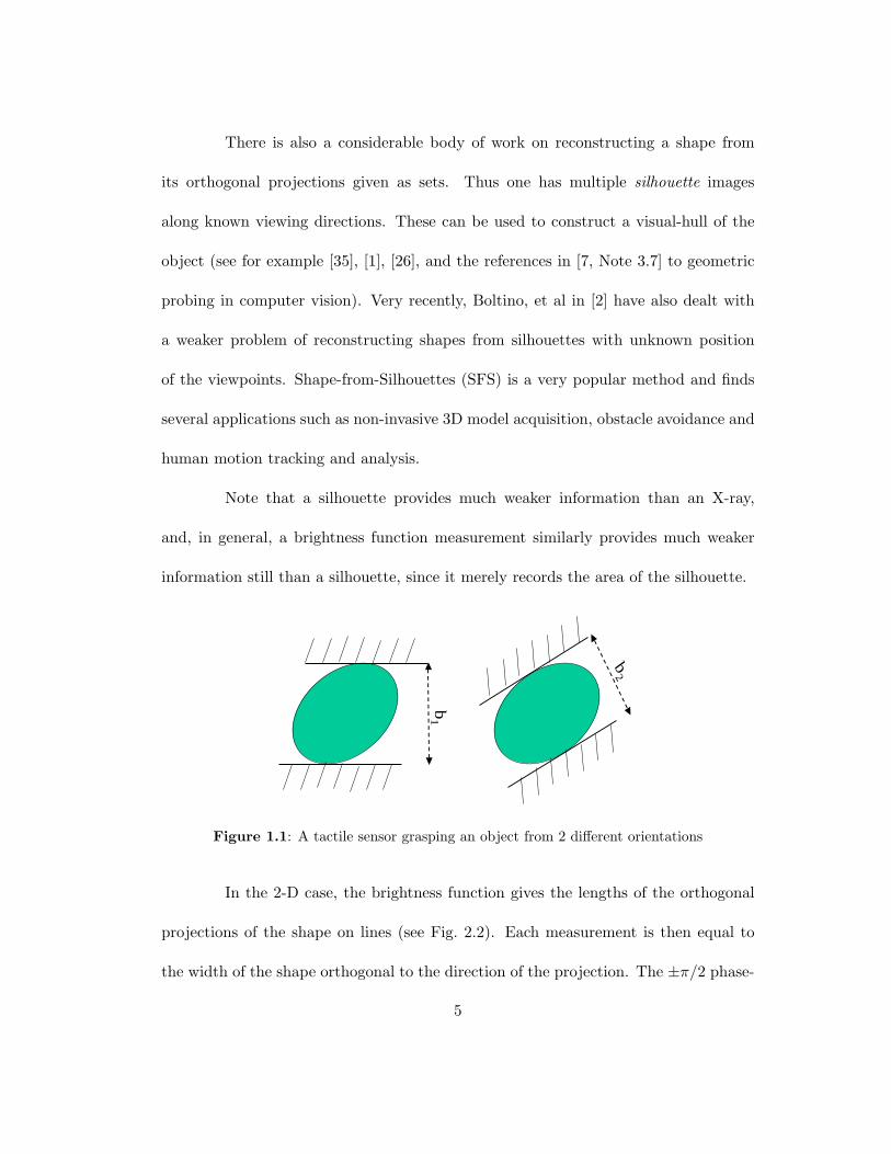
Figure 1.1: A tactile sensor grasping an object from 2 different orientations
In the 2-D case, the brightness function gives the lengths of the orthogonal
projections of the shape on lines (see Fig. 2.2). Each measurement is then equal to
the width of the shape orthogonal to the direction of the projection. The ±π/2 phase-
5

shifted version of brightness function in the planar case is referred to as the diameter
function or width function in the robotics and computer vision community. Diameter
measurements can also be obtained as the sum of support-line measurements along
two antipodal directions. Shape from diameter has also been extensively studied by
the robotics community where the diameter of an object can be measured using an
instrumented parallel jaw-gripper as in Fig. 1.1). Rao and Goldberg [38] observed that
diameter cannot be used to uniquely reconstruct shapes; instead they used them for
recognizing a shape from a known (finite) set of shapes. Lindenbaum and Bruckstein
[30] showed that shape can be uniquely reconstructed from binary perspective projec-
tions using 3V − 3 measurements and proved this to be optimal. However, as with
support functions, this work assumes pure measurements and pays more attention to
algorithmic complexity.
1.3 Thesis Contribution and Organization
This thesis addresses the problem of reconstructing the shape of a planar
convex object from finite, noisy and possibly sparse measurements of the support and
brightness functions along a known set of viewing directions. Though this is not valid
for higher dimensions, we shall collectively refer to support, diameter and brightness
functions as support-type data. The shape is parameterized using its Extended Gaus-
sian Image (EGI) because this parameterization facilitates a systematic statistical
analysis of the problem. Using EGI, a polygon is encoded in terms of the lengths ak
6
of its edges and their outer normal angles θk.
The thesis addresses two important aspects of the two inverse problems under
consideration. First, we focus on non-linear and linear estimation algorithms for re-
constructing shape from noisy support-type data. For support function measurements
our approach is novel in that the approximating shape, a convex polygon, is param-
eterized using its Extended Gaussian Image (EGI). Second, we present a systematic
statistical analysis of the problem via the Cramer-Rao lower bound and confidence
region analysis. As a byproduct of the statistical analysis, we also introduce for the
first time, a correct method for reconstructing planar shapes using corrupted EGI.
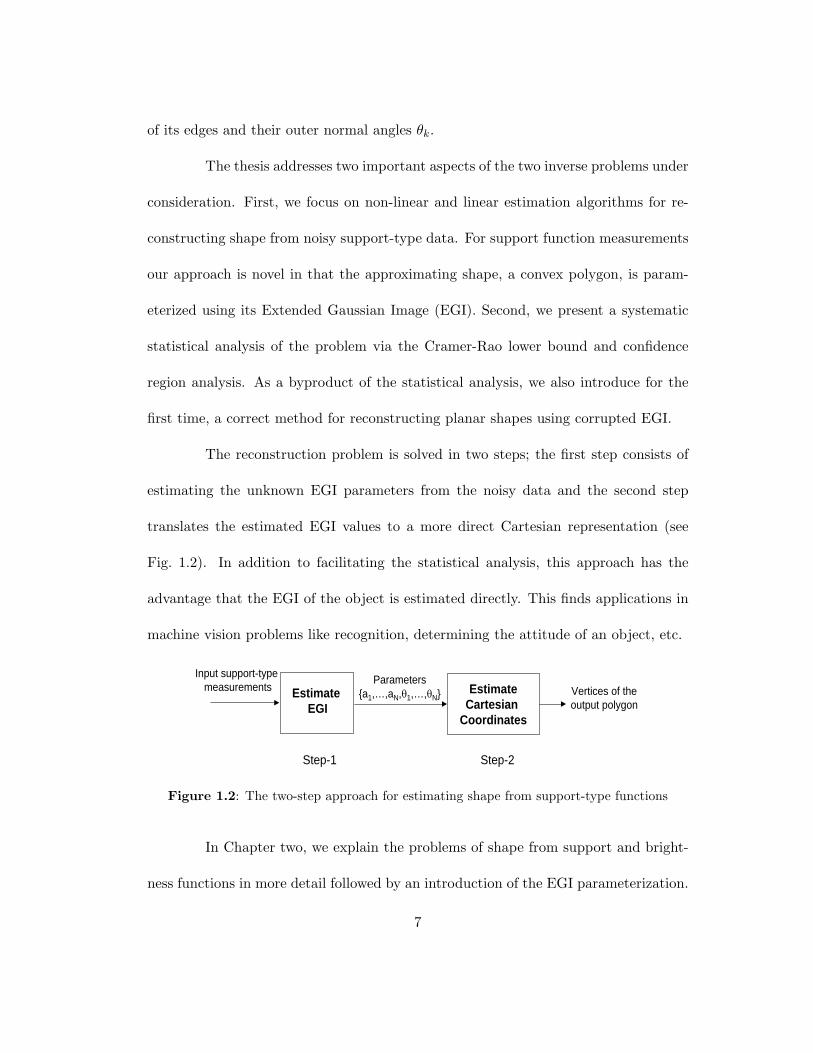
The reconstruction problem is solved in two steps; the first step consists of
estimating the unknown EGI parameters from the noisy data and the second step
translates the estimated EGI values to a more direct Cartesian representation (see
Fig. 1.2). In addition to facilitating the statistical analysis, this approach has the
advantage that the EGI of the object is estimated directly. This finds applications in
machine vision problems like recognition, determining the attitude of an object, etc.
Input support-typemeasurements Estimate
CartesianCoordinates
Step-1 Step-2
Parametersa1,…,aN, 1,…, NEstimate
EGIVertices of theoutput polygon
Figure 1.2: The two-step approach for estimating shape from support-type functions
In Chapter two, we explain the problems of shape from support and bright-
ness functions in more detail followed by an introduction of the EGI parameterization.
7
The second step in Fig. 1.2, addressing the inverse problem of finding a shape from its
EGI, is of considerable interest in its own right. Applications include astrophysics [25],
computer vision [28], [32], the reconstruction of a cavity from ultrasound [41], and esti-
mation of the directional distribution of a fiber process [24]. At first sight the problem
seems a trivial one in the 2-D case, but the obvious method described in Section 2.3
was shown by our statistical study to be unsatisfactory. A completely new method we
claim to be the correct one is introduced in Section 2.3.1. The same problem in three
dimensions remains open. Finally in Section 2.4 we define the mathematical model
for support-type measurements under the EGI parameterization.
Chapter three starts with a discussion of the previous algorithms for shape re-
construction from corrupted support function measurements. We propose novel linear
and non-linear estimation algorithms for shape estimation using support-line measure-
ments under the EGI parameterization. In Section 3.3 is a discussion of algorithms
for reconstruction from noisy brightness function data. For exact measurements, these
were introduced by Gardner and Milanfar [9], [10] and were proved in [10] to converge
in any dimension when the convex body is origin symmetric, a requirement needed
for uniqueness. By “converge,” we mean that the outputs of the algorithms converge
in the Hausdorff metric to the input convex body as the number of measurement di-
rections increases through a sequence of directions whose union is dense in the unit
sphere. In forthcoming joint work with Kiderlen [8], it will be shown that these al-
gorithms, as well as those using the support function, still converge with noisy data.
(Such convergence results seem to be rare. In particular, the algorithm in [6] is only
8

proved to converge with probability approaching one as the number of measurement
directions increases.) In this sense the algorithms we present are fully justified.
In Chapter five, we present sample output reconstructions obtained using the
algorithms discussed in Chapter four for both support and brightness function mea-
surements. We study the effect of experimental parameters like noise power, number
of measurements, eccentricity and scale of the underlying polygon, on the quality of
the estimated shape using Monte-Carlo simulations.
The statistical analysis itself is presented in Chapter five. Again, the ap-
proach for this type of reconstruction problem is new, involving the derivation of the
constrained Cramer-Rao lower bound (CCRLB) on the estimated parameters. Using
the CCRLB, local and global confidence regions can be calculated corresponding to
any preassigned confidence level. These form uncertainty regions around points in the
boundary of the underlying object, or around its whole boundary. Such confidence re-
gions are tremendously powerful in displaying visually the dependence of measurement
direction set, noise power, and the eccentricity, scale, and orientation of the underlying
true shape on the quality of the estimated shape.
The confidence regions also assist us in doing a statistical performance analy-
sis of the proposed algorithms which is presented in Chapter six. Performance analysis
can be carried out using either local confidence regions as in Section 6.1 or using global
confidence regions as in Section 6.2. We also present some more experimental results
of the reconstructed polygons together with their local and global confidence regions
in this section.
9

Finally, in Chapter seven, we introduce another exciting inverse problem
called shape from lightness functions which forms an interesting direction of future
research, and we present conclusive remarks for this thesis.
10

Chapter 2
Support-type functions and the
EGI
In this chapter, we discuss the mathematical models for support and brightness func-
tion measurements. We introduce the EGI (Extended Gaussian Image) parameteri-
zation of a 2-D shape and also define support and brightness function data using the
EGI parameterization.
2.1 Background
The support line LS(α) of the convex set S at angle α is a line orthogonal
to the unit vector v = [cos(α), sin(α)]T that just grazes the set S such that the shape
lies completely in one of the half-planes defined by LS(α) (see Fig. 2.1). Its equation
is given as,
LS(α) = x ∈ <2|xTv = hS(α), (2.1)
11
where,
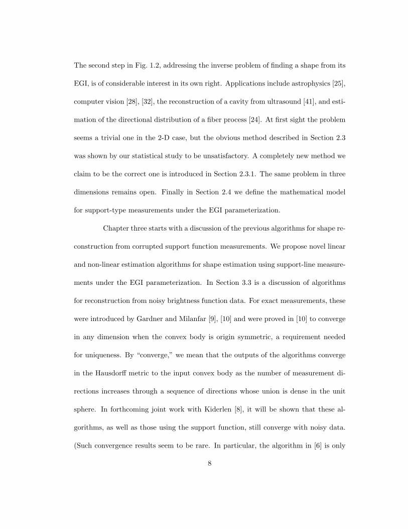
hS(α) = supx∈S
xTv. (2.2)
The magnitude of support function, i.e., |hS(α)| is the minimum distance from the
origin to the support line LS(α).
S
v
x
y
Ls( )
h()
O
Figure 2.1: Support-line measurementof a planar body.
v
x
Ls( )
y
Ls( + )w(
)
-v
Figure 2.2: Diameter measurement of aplanar body.
hS(α) is continuous and periodic with period 2π. A convex set can be com-
pletely determined by its support function measurements obtained from all viewing
directions ([39], p. 38). However in practice, we only have a finite number of support
function measurements h = [h(α1), h(α2), . . . , h(αM )]T . Therefore there is a family of
sets having the same support vector h. The largest of these sets, a polygon SP, that
is uniquely determined by h can be obtained by the intersection of the half-planes
defined by support-lines as follows,
SP = x ∈ <2|xT [v1,v2, . . . ,vM ] ≤ [h1, h2, . . . , hM ]. (2.3)
If zt = (xt, yt) for t = 1, . . . , N are the vertices of the N-sided convex polygon SP, the
12
support function
hSP(α) = maxt(xt cosα + yt sinα). (2.4)
For planar shapes, another closely related measurement is its width function.
The width function is calculated as the sum of support-line measurement along two
antipodal directions (see Fig. 2.2), i.e.,
w(α) = h(α) + h(α + π). (2.5)
Thus the width function is continuous and periodic with a period of π. The brightness
function is simply a phase shifted version of the width function,
b(α) = w(α + π/2) = h(α + π/2) + h(α− π/2). (2.6)
Therefore, in the planar case, the brightness function measures the length of
the orthogonal projection (silhouette) of the shape. Each measurement b(α) provides a
single scalar that records the length of the silhouette viewed from angle α and nothing
at all about its position. Whereas a planar convex body is uniquely determined by
all its silhouettes, there can be infinitely many number of bodies having the same
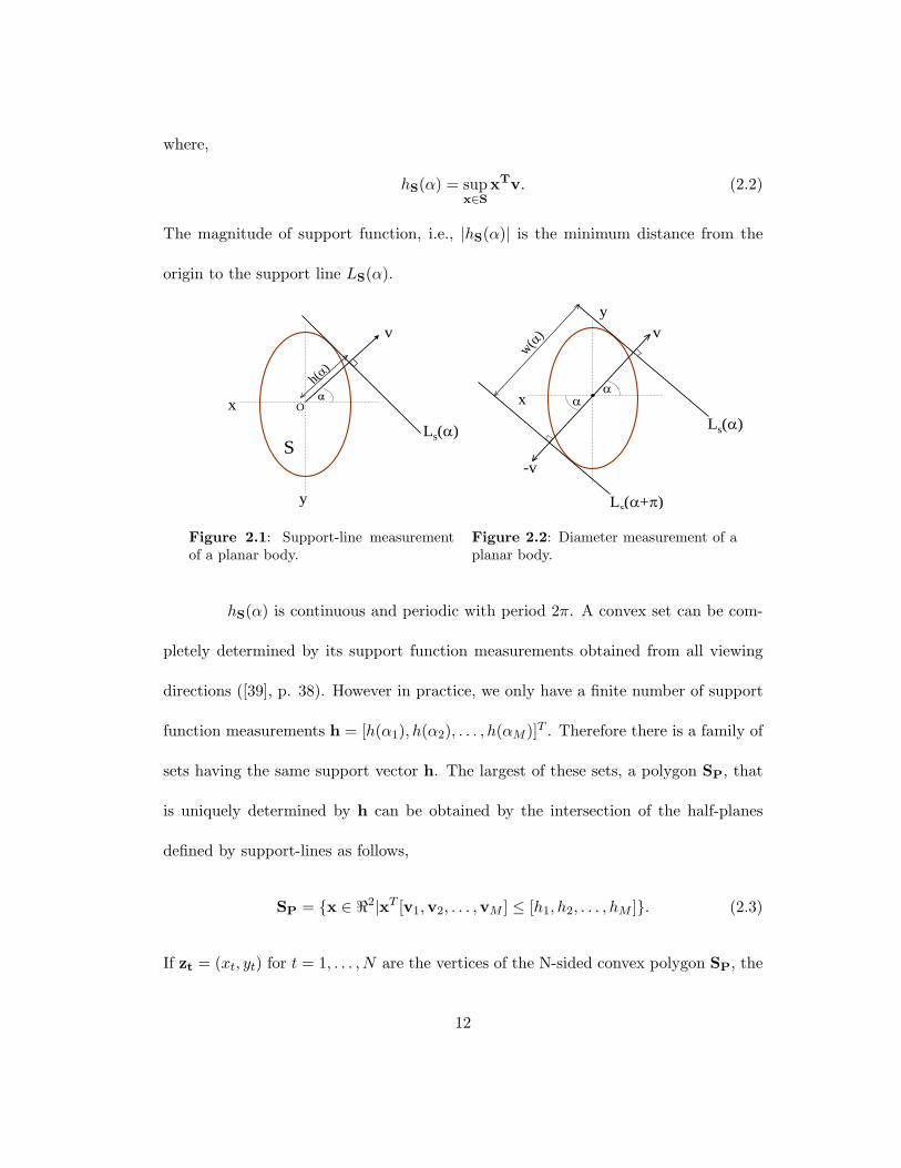
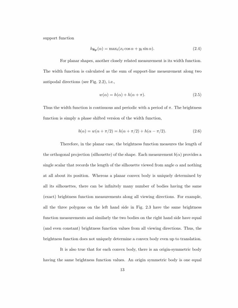
(exact) brightness function measurements along all viewing directions. For example,
all the three polygons on the left hand side in Fig. 2.3 have the same brightness
function measurements and similarly the two bodies on the right hand side have equal
(and even constant) brightness function values from all viewing directions. Thus, the
brightness function does not uniquely determine a convex body even up to translation.
It is also true that for each convex body, there is an origin-symmetric body
having the same brightness function values. An origin symmetric body is one equal
13
Figure 2.3: Non-uniqueness issue with brightness functions.
to its reflection in the origin. For detailed discussions, see [7, Chapter 3] and [10].
However, a remarkable result due to Alexandrov [7, Theorem 3.3.6] called Alexan-
drov’s projection theorem, states that any two origin-symmetric convex bodies having
the same brightness function must be equal. By seeking to reconstruct only origin-
symmetric bodies, we therefore overcome the non-uniqueness problem for brightness
functions. For example, in Fig. 2.3 the hexagon and the circle are origin symmetric
bodies and hence our algorithm reproduces them uniquely as outputs.
2.2 Extended Gaussian Image
Underlying our whole approach is the idea of parameterizing a shape using
its Extended Gaussian Image (EGI), also referred to as the Extended Circular Image
in the 2-D case. EGI is obtained by mapping the surface normal vector information
of an object onto the unit sphere (the unit circle in the 2-D case) called the Gaussian
sphere. Each region of the unit sphere (unit circle in 2-D) is assigned a weight equal
to the area (length in 2D) of the set of points on the surface of the shape at which the
14

outer unit normal vector lies in the region. The EGI has the desirable property that
it determines a convex object uniquely (up to translation). For more details, we refer
the reader to [39] and [18].
When the shape is a suitably smooth convex body, the EGI can be represented
by a function f(u), where u is a unit vector and f(u) is the reciprocal of the Gaussian
curvature of the surface of the body at the point where the outer unit normal is u; see
[10]. Thus in effect the EGI encodes the shape in terms of its curvature as a function
of the outer unit normal to its boundary.
1
2
3
4
a1u1
a4u4
a2u2
a3u3
Figure 2.4: EGI vectors of a polygon.
When the shape is a convex polygon (or more generally, an n-dimensional
convex polyhedron), the EGI is simple to describe. For an N -sided polygon whose
kth edge has length ak and outer unit normal vector uk, the EGI is a measure on the
unit circle consisting of a finite sum of point masses, each placed at the outer unit
normal to an edge and having weight equal to the length of that edge. In other words,
it becomes
f(u) =N∑
k=1
akδ(u− uk), (2.7)
where δ is the Dirac delta function. As Fig. 2.4 indicates, the EGI of an N-sided
15
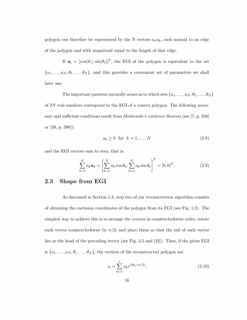
polygon can therefore be represented by the N vectors akuk, each normal to an edge
of the polygon and with magnitude equal to the length of that edge.
If ui = [cos(θi), sin(θi)]T , the EGI of the polygon is equivalent to the set
a1, . . . , aN , θ1, . . . , θN, and this provides a convenient set of parameters we shall
later use.
The important question naturally arises as to which sets a1, . . . , aN , θ1, . . . , θN
of 2N real numbers correspond to the EGI of a convex polygon. The following neces-
sary and sufficient conditions result from Minkowski’s existence theorem (see [7, p. 356]
or [39, p. 390]):
ak ≥ 0 for k = 1, . . . , N (2.8)
and the EGI vectors sum to zero, that is,
N∑
k=1
akuk =
[N∑
k=1
ak cos θk,N∑
k=1
ak sin θk
]T
= [0, 0]T . (2.9)
2.3 Shape from EGI
As discussed in Section 1.3, step two of our reconstruction algorithm consists
of obtaining the cartesian coordinates of the polygon from its EGI (see Fig. 1.2). The
simplest way to achieve this is to arrange the vectors in counterclockwise order, rotate
each vector counterclockwise by π/2, and place them so that the tail of each vector
lies at the head of the preceding vector (see Fig. 2.5 and [32]). Then, if the given EGI
is a1, . . . , aN , θ1, . . . , θN, the vertices of the reconstructed polygon are
zt =t∑
k=1
akei(θk+π/2), (2.10)
16
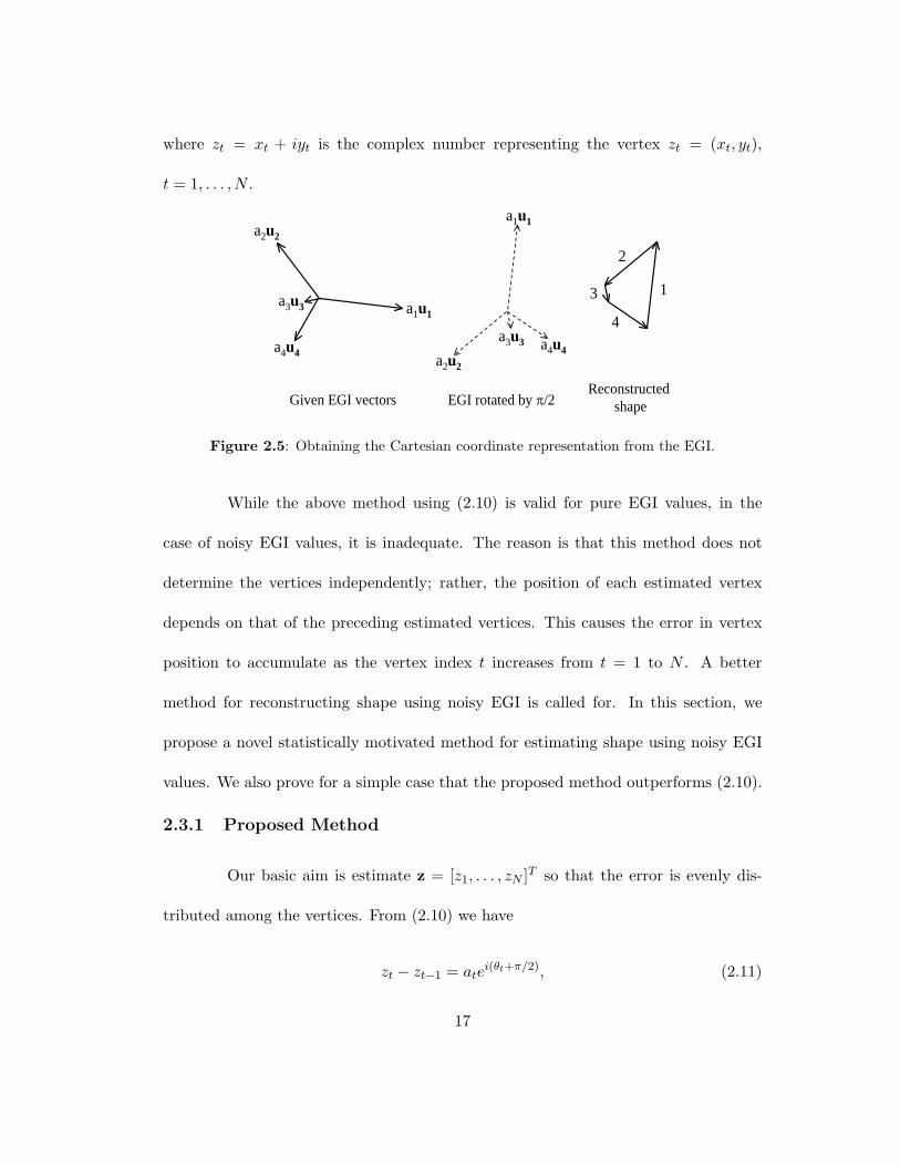
where zt = xt + iyt is the complex number representing the vertex zt = (xt, yt),
t = 1, . . . , N .
Given EGI vectors
1
EGI rotated by /2Reconstructed
shape
a1u1
a4u4
a2u2
a3u3
2
3
4
a1u1
a2u2
a3u3 a4u4
Figure 2.5: Obtaining the Cartesian coordinate representation from the EGI.
While the above method using (2.10) is valid for pure EGI values, in the
case of noisy EGI values, it is inadequate. The reason is that this method does not
determine the vertices independently; rather, the position of each estimated vertex
depends on that of the preceding estimated vertices. This causes the error in vertex
position to accumulate as the vertex index t increases from t = 1 to N . A better
method for reconstructing shape using noisy EGI is called for. In this section, we
propose a novel statistically motivated method for estimating shape using noisy EGI
values. We also prove for a simple case that the proposed method outperforms (2.10).
2.3.1 Proposed Method
Our basic aim is estimate z = [z1, . . . , zN ]T so that the error is evenly dis-
tributed among the vertices. From (2.10) we have
zt − zt−1 = atei(θt+π/2), (2.11)
17
for t = 1, . . . , N , and hence the equation
Qz = r, (2.12)
where
Q =
−1 1 0 · · · 0 0
0 −1 1 · · · 0 0
......
......
...
0 0 0 · · · −1 1
1 0 0 · · · 0 −1
(2.13)
and
r =[a1e
i(θ1+π/2), . . . , aNei(θN+π/2)]T
.
However, rankQ = N − 1 and so the solution for z in (2.12) is not unique. We
overcome this by fixing the barycenter of the vertices of the polygon (that is, their
average) at the point with complex number form c by adding the constraint
N∑
t=1
zt = c. (2.14)
When c is the origin, this can be written in the form eT z = 0, where e = [1, 1, . . . , 1]T .
We can now solve the well-defined least-squares problem,
minz‖Qz− r‖2 + (eTz)2. (2.15)
The solution is a point where the derivative of the cost function becomes zero. There-
fore,
d
dz
(||Qz− r||2 + (eTz)2
)=
d
dz
(zTQTQz− 2zTQTr + rTr + zeeTz
)= 0. (2.16)
18

This yields the unique solution,
z = (QTQ + eeT )−1QT r = Dr, (2.17)
where we note that the matrix being inverted is now full rank. Let dij for i, j =
1, . . . , N represent the elements of the matrix D. Therefore,
zt =N∑
k=1
dtkakei(θk+π/2), (2.18)
for t = 1, . . . , N . Comparing (2.18) with (2.10), we see that zt now depends on all the
EGI vectors.
2.3.2 A basic statistical comparison of the two methods
From Fig. 1.2 we note that the EGI is estimated from the noisy input support-
type data and therefore it too will be corrupted. Let a = [a1, . . . , aN ]T and Θ =
[θ1, . . . , θN ]T correspond to the estimated EGI components. For the sake of simplicity
in our analysis, let us assume that the angles are estimated accurately, i.e. Θ = Θ,
thereby leaving a as the only corrupted data. We further assume that the elements of
a have identical variances and are uncorrelated to each other. Then the covariance of
a is
cov(a) =
σ2 0 0 · · · 0
0 σ2 0 · · · 0
......
......
0 0 0 · · · σ2
= σ2I. (2.19)
19
From (2.10), the estimated polygon z is given as,
z = Pr (2.20)
where,
P =
1 0 0 · · · 0 0
1 1 0 · · · 0 0
...
1 1 1 · · · 1 1
(2.21)
and,
r =[a1e
i(θ1+π/2), a2ei(θ2+π/2), . . . , aNei(θN+π/2)
]T. (2.22)
Now, cov(z) = Pcov(r)PT. Hence, our next task is to calculate the covari-
ance of r. We note that r can be written as,
r =
ei(θ1+π/2) 0 · · · 0 0
0 ei(θ2+π/2) · · · 0 0
...
0 0 · · · ei(θN−1+π/2) 0
0 0 · · · 0 ei(θN+π/2)
a1
a2
...
aN−1
aN
= RΘa
(2.23)
Therefore,
cov(r) = RΘcov(a)RΘH
= RΘRΘHcov(a) (cov(a) and RΘ are diagonal matrices)
20

= (I) cov(a) (RΘ is a unitary matrix)
= σ2I (from 2.19) (2.24)
Therefore,
cov(z) = σ2(PPT) (2.25)
The variances of the individual estimated vertices are given by the diagonal elements
of the above matrix. By observing the structure of the matrix P, it is not difficult to
see that these diagonal elements are increasing linearly as a function of the index t.
More explicitly,
PPT =
1 1 1 · · · 1
1 2 2 · · · 2
1 2 3 · · · 3
......
......
1 2 3 · · · N
,
which leads to,
var(zt) =t∑
i=1
σ2 (2.26)
for t = 1, . . . , N
Equation (2.26) clearly demonstrates that the variance of the estimated ver-
tex increases as the index increases (accumulation effect). This is highly undesirable
and therefore (2.10) is not an optimum method for estimating cartesian coordinates
from EGI.
21
Next we demonstrate that the proposed method (2.18) overcomes this is-
sue. From (2.17), z = D.r, therefore, cov(z) = Dcov(r)DT. Employing the same
assumptions and arguments as earlier, we note that,
cov(z) = σ2(DDT) = σ2(QTQ + eeT )−1QTQ(QTQ + eeT )−1. (2.27)
By (2.13), Q is a square circulant matrix, and since e = [1, 1, . . . , 1]T , the
matrix eeT has every entry equal to 1 and is therefore also a square circulant matrix.
Using the well-known facts that the sum, product, transpose, and inverse of square
circulant matrices are again square circulant matrices [4], we see from (2.27) that
cov(z) is also a square circulant matrix. Therefore its diagonal elements are equal;
in other words, the variances var(zt), t = 1, . . . , N are all equal and hence the er-
ror is distributed more evenly amongst all the vertices. Moreover, the variances are
independent of the index number of the vertices unlike (2.26).
Under our simplifying assumption, this demonstrates that the proposed method
(2.18) is a statistically improved way of estimating the cartesian coordinates of a poly-
gon from the corrupted EGI values. However, an extension of this problem to the 3-D
case is more difficult. Little in [32] proposed a non-linear algorithm for reconstructing
a 3-D shape from pure EGI values. The problem of 3-D shape reconstruction from
noisy EGI has essentially not been treated by researchers in the past (so far as we are
aware), thereby forming a challenging direction of future work.
22
2.4 Relation between support-type functions and the EGI
Here we define the mathematical model which will enable us to directly cal-
culate the support and brightness function values of a shape from the EGI.
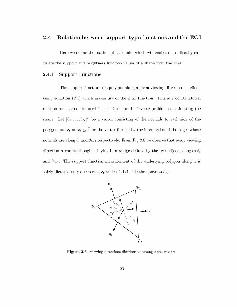
2.4.1 Support Functions
The support function of a polygon along a given viewing direction is defined
using equation (2.4) which makes use of the max function. This is a combinatorial
relation and cannot be used in this form for the inverse problem of estimating the
shape. Let [θ1, . . . , θN ]T be a vector consisting of the normals to each side of the
polygon and zt = [xt, yt]T be the vertex formed by the intersection of the edges whose
normals are along θt and θt+1 respectively. From Fig 2.6 we observe that every viewing
direction α can be thought of lying in a wedge defined by the two adjacent angles θt
and θt+1. The support function measurement of the underlying polygon along α is
solely dictated only one vertex zt which falls inside the above wedge.
z1
z2
z3
v1
v3
v4
v2
v5
v6
u1
u2
u3
Figure 2.6: Viewing directions distributed amongst the wedges.
23
Thus, if θt ≤ α < θt+1, (2.4) can be simplified as,
hS(α) = xt cos(α) + yt sin(α). (2.28)
Note that if we first assign the correspondence between the viewing angles and the
wedges formed by the normals, we can get rid of the max function in (2.4). Using
(2.18), we can write the vertex coordinates zt = [xt, yt]T of a polygon in terms of its
EGI as follows,
zt =
[N∑
k=1
dtkak cos(θk + π/2),N∑
k=1
dtkak sin(θk + π/2)
]T
. (2.29)
From (2.29) and (2.28) we obtain,
hS(α) =N∑
k=1
dtkak cos(θk + π/2) cos(α) +N∑
k=1
dtkak sin(θk + π/2) sin(α),
=N∑
k=1
dtkak sin(α− θk). (2.30)
Note that the above expression is only valid for a polygon having the barycen-
ter of its vertices at the origin. Thus, the support values of a polygon can be calculated
from its EGI using (2.30).
2.4.2 Brightness Functions
We now proceed to defining the brightness function values of a shape using
EGI. The brightness function b(v) of a continuous body for a given viewing direction
v (a unit vector) is given by [7],
b(v) =12
∫
S|uT v|f(u)du. (2.31)
24

Integration is over the unit sphere (in two dimensions, the unit circle S). Since |uT v| is
a cosine term, it is true that |uT v|f(u)du represents the area of the projection in the
direction v of an surface element du normal to u (refer Fig. 2.7). Thus, the brightness
function measurement along a given direction is the volume of the orthogonal pro-
jection of the body along that direction. It is important to note that the brightness
functions data are scalar values (volume of projections), therefore they only provide a
one-dimensional information about an n-dimensional body. As a result the brightness
function data becomes progressively weaker as we move on to the higher dimensions.
Figure 2.7: A 3-D object and its shadowin the direction v.
αθk
ak|cos(α - θ
k )|
Figure 2.8: Projection of an edge.
For an N-sided convex polygon, ak|uTk v| is just the length of the projection of
the kth edge in the direction v (see Fig. 2.8). The brightness function of this polygon
is
b(v) =12
N∑
k=1
ak|uTk v|. (2.32)
(This formula can also be obtained by substituting (2.7) into (2.31), assuming this is
valid.) If v = [cosα, sinα]T and uk = [cos θk, sin θk]T , we can rewrite (2.32) in the
25

form
b(α) =12
N∑
k=1
ak| cos(α− θk)|. (2.33)
Thus, the brightness function values of a polygon can be calculated from its EGI using
(2.33). We note here that b(α) can also be thought of as the circular convolution of
the vector a with the function |cos(x)|.
26

Chapter 3
Algorithms for shape fromsupport-type functions
In this chapter, we propose linear and non-linear algorithms for estimating the EGI of
a polygon from finite and noisy support-type measurements. We follow the two step
approach for shape reconstruction outlined in Fig. 1.2.
3.1 Support functions
We consider an unknown planar convex body K with a finite number of noisy
support function measurements modelled by, y(αm) = h(αm)+n(αm) in fixed measure-
ment directions vm = [cos αm, sinαm]T , m = 1, . . . , M . The noise n(αm) is assumed
to be white Gaussian noise with variance σ2. Collecting the above measurements into
a vector form,
y = h + n, (3.1)
where y = [y(α1), . . . , y(αM )]T is the observation vector, h = [h(α1), . . . , h(αM )]T is
the vector of true support values and n = [n(α1), . . . , n(αM )]T is the noise vector. We
27

now discuss some past algorithms for shape reconstruction from corrupted support
function data.
3.1.1 Past Algorithms
Prince and Willsky [37] observed that because of the presence of noise, the
measured support vector y = [y(α1), . . . , y(αM )]T may not correspond to any closed
convex set S. They derived the necessary and sufficient conditions, a set of inequality
constraints, to check the consistency of the measured support vector y when the
measurement angles are equally spaced. Lele, et al [27] extended their work by deriving
the constraint set for the more practical case of any general measurement set.
Using (3.1), the estimated vector h can be obtained by employing the con-
strained linear least squares optimization as (see [27]),
h = arg minh||y − h||2, (3.2)
subject to the constraint,
C(Ω)h ≥ 0 (3.3)
where Ω = [α1, . . . , αM ]T and,
C(Ω) =
− sin(α2 − αM ) sin(α1 − αM ) 0 . . . sin(α2 − α1)
sin(α3 − α2) − sin(α3 − α1) sin(α2 − α1) . . . 0
0 sin(α4 − α3) − sin(α4 − α2) . . . 0
......
......
...
sin(αM − αM−1) 0 0 sin(α1 − αM ) − sin(α1 − αM−1)
.
(3.4)
The constraint (3.3) is a necessary and sufficient condition, essentially due to Rademacher
(see [39, p. 47], which includes an extension to higher dimensions), for h to be con-
28

sistent with a support function of a closed convex set. From h, the output polygon
can be reconstructed using the intersection method described in (2.3). Note that this
method gives an M -sided output polygon irrespective of the number of sides of the
underlying polygon.
The second method proposed by Lele, Kulkarni and Willsky in [27] makes use
of prior information about the angles of sides of the object. The aim is to reconstruct
an N -sided polygon with pre-specified normal directions to its sides using M corrupted
support function measurements. Let θ1, . . . , θN be the known angles of the sides of
the underlying polygon. The shape is parameterized using its support function values
at Θ where Θ = [θ1, . . . , θN ]T . Hence, if a given measurement angle αm lies anywhere
in the wedge formed by two adjacent normals θLm and θRm , i.e. θRm ≤ αm ≤ θLm ,
then,
h(αm) =sin(θRm − αm)sin(θRm − θLm)
hLm +sin(αm − θLm)sin(θRm − θLm)
hRm . (3.5)
The support function measurement model in this case is,
y = A(Θ)h + n, (3.6)
where, y and n hold the same meaning as in (3.1) but h = [h(θ1), h(θ2), . . . , h(θN )]T .
The matrix A(Θ) ∈ <M×N is defined using (3.5) which computes the support values
along any direction α using the support values along two adjacent normals. Thus the
mth row of A(Θ) has two adjacent non-zero entries corresponding to angles θLm and
θRm such that αm lies in the interval [θLm , θRm ]. Using (3.6), the estimated vector h
29

can be obtained by employing least squares optimization (see [27]),
h = arg minh||y −A(Θ)h||2, (3.7)
subject to the constraint C(Θ) ≥ 0. The matrix A(Θ) in (3.7) is completely deter-
mined and hence the optimization problem is linear in the unknown parameter h.
3.1.2 Proposed Algorithms using EGI Parameterization
We use the two-step approach outlined in Fig. 1.2 to estimate shape from
noisy support functions. In this section we discuss algorithms for estimating the EGI
of a convex polygon using finite, noisy support line measurements. Once this is done,
we can use (2.18) to obtain the cartesian coordinates of the polygon.
Here we deal with two cases; in the first case, the normal to the edges are
either known or fixed a priori and therefore we estimate only the length of edges,
whereas, in the second case the entire EGI vector (both length and normals) are
estimated. The estimation algorithms are linear and non-linear for the aforementioned
cases respectively.
Linear Algorithms
If we assume that the underlying shape K is an N -sided polygon whose
vertices have barycenter at 0 and which has prescribed outer normal angles θk, k =
1, . . . , N , then we proceed as follows. For each measurement angle αm, we assign tm
30

such that θtm ≤ αm < θtm+1 and then use (2.30) and (3.1) to obtain
y(αm) =N∑
k=1
dtmkak sin(αm − θk) + n(αm), (3.8)
where the unknowns are the edge lengths ak, k = 1, . . . , N . In vector form this becomes
the measurement model
y = S(Θ)a + n, (3.9)
where y, Θ, and n have the same meaning as in (3.6), a = [a1, . . . , aN ]T , and the
matrix S(Θ) ∈ <M×N has entries S(Θ)m,k = dtmk sin(αm − θk). We can then solve
the least squares problem
a = arg mina||y − S(Θ)a||2, (3.10)
subject to the Minkowski’s condition give by (2.8) and (2.9) which ensure that the
estimated EGI vector corresponds to a closed convex polygon. Since Θ is known, S(Θ)
is completely determined and the constraints are linear in the unknown parameter a;
hence (3.10) is a constrained linear least squares optimization problem.
The linear algorithm based on (3.10) is equivalent to that of Lele, Kulkarni,
and Willsky [27] described in (3.7); that is, for a given input vector y and prescribed
outer normal angle vector Θ, the outputs of the two algorithms are the same (provided
both algorithms construct polygons whose vertices have barycenter at 0). If we take
N = M and replace Θ by Ω, the algorithm based on (3.10) is equivalent to that of
Prince and Willsky [37] described in (3.2).
31
Non-linear algorithm
In this case, both normals and length of edges of the underlying polygon
are unknown. However, we assume that the underlying polygon has its barycenter at
the origin and that the correspondence between the viewing angles and the wedges (as
explained in Fig. 2.6 and Section 2.4.1) is known a priori. Thus, for every measurement
αm, we know tm such that θtm ≤ αm ≤ θtm+1. Under these assumptions, we can write
the measurement model using (3.8) as,
y = S(Θ)a + n. (3.11)
However, in this case the unknowns are a1, . . . , aN and θ1, . . . , θN . Note that our
prior assumption is weaker compared to Lele, et al in (3.6); they assumed that the
normal directions of the edges are pre-specified, whereas in our case the normals are
still unknown. Also, unlike (3.2), the number of sides of the reconstructed polygon are
independent of the number of measured support values.
Employing the least-squares error criterion, the unknowns in (3.11) can be
estimated as,
(a, Θ) = arg min(a,Θ)
||y − S(Θ)a||2 (3.12)
subject to the Minkowski constraints (2.8) and (2.9). Note that the optimization
problem is non-linear in the unknown parameters. Moreover, this algorithm is actually
the Maximum Likelihood Estimator (MLE) of the unknown parameters a and Θ owing
to the Gaussian noise assumption (see [23, pp. 223–6 and 254–5] for further details).
32

3.2 Algorithms for Shape from Brightness Functions
We now discuss algorithms for shape reconstruction using corrupted bright-
ness function measurements. The problem is solved using the same two-step approach
illustrated in Fig. 1.2. In this section we discuss linear and non-linear algorithms to
estimate the EGI of a polygon from corrupted brightness function data.
We assume that the brightness function measurements are obtained from an
N -sided polygon using the model b(αm) = b(αm) + n(αm), m = 1, . . . , M , where the
first term is given by (2.33) and the second term is the noise. As before, the noise
throughout the discussion is Gaussian white noise with variance σ2. While the scope
of this section is restricted to the planar case, the algorithms discussed in this section
can be readily extended to higher dimensions (for more details see [10]).
In vector form the measurements are
b = C(Θ)a + n, (3.13)
where b = [b(α1), . . . , b(αM )]T , n = [n(α1), . . . , n(αM )]T , a = [a1, . . . , aN ]T , Θ =
[θ1, . . . , θN ]T , and C(Θ)mk = | cos(αm − θk)|/2. Employing the least-squares error
criterion, the unknowns in (3.13) can be estimated as
(a, Θ) = arg min(a,Θ)
‖b−C(Θ)a‖2. (3.14)
However, note that a and Θ should define a convex polygon, therefore the optimization
problem (3.14) is subject to the constraints (2.8) and (2.9).
In general, the solution to (3.14) is not unique, even when there is no noise
33

in the measurements. This is to be expected in view of the, finite, weak nature of
data. But in order to ensure a reasonable reconstruction, we also need to overcome
the more serious non-uniqueness issue associated with brightness functions illustrated
by Fig. 2.3. As per our discussion in Section 2.1, this can be achieved if we seek to
reconstruct origin-symmetric convex bodies. The origin symmetry of our approximat-
ing polygon is ensured by imposing the following linear constraints on its EGI (note
that N must be even in this case):
ak = aN/2+k for k = 1, . . . , N/2; (3.15)
θk = θN/2+k + π for k = 1, . . . , N/2. (3.16)
These two constraints imply (2.9) and hence make it redundant. To sum-
marize, we solve (3.14), subject to (2.8), (3.15), and (3.16). This algorithm is the
Maximum Likelihood Estimator (MLE) of the unknown parameters a and Θ again
owing to the Gaussian noise assumption. Since (3.14) is non-linear in the unknown
parameters, constrained non-linear optimization is required, and this is computation-
ally very expensive. Without adaptation, this algorithm is therefore of little practical
use.
One possible adaptation is prompted by the observation that the least squares
problem (3.14) is of a special type known as separable. It could then be feasible to use
the variable projection method of Golub and Pereyra [12] where each of the unknowns
a and Θ is treated separately in each iteration. However, a different modification, using
a theoretical result of Campi, Colesanti, and Gronchi [3], effectively allows (3.14) to be
34
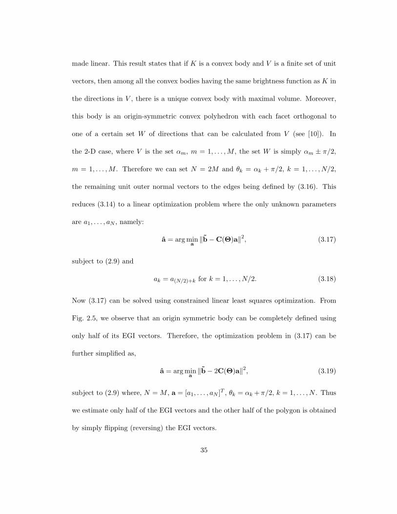
made linear. This result states that if K is a convex body and V is a finite set of unit
vectors, then among all the convex bodies having the same brightness function as K in
the directions in V , there is a unique convex body with maximal volume. Moreover,
this body is an origin-symmetric convex polyhedron with each facet orthogonal to
one of a certain set W of directions that can be calculated from V (see [10]). In
the 2-D case, where V is the set αm, m = 1, . . . , M , the set W is simply αm ± π/2,
m = 1, . . . , M . Therefore we can set N = 2M and θk = αk + π/2, k = 1, . . . , N/2,
the remaining unit outer normal vectors to the edges being defined by (3.16). This
reduces (3.14) to a linear optimization problem where the only unknown parameters
are a1, . . . , aN , namely:
a = arg mina‖b−C(Θ)a‖2, (3.17)
subject to (2.9) and
ak = a(N/2)+k for k = 1, . . . , N/2. (3.18)
Now (3.17) can be solved using constrained linear least squares optimization. From
Fig. 2.5, we observe that an origin symmetric body can be completely defined using
only half of its EGI vectors. Therefore, the optimization problem in (3.17) can be
further simplified as,
a = arg mina‖b− 2C(Θ)a‖2, (3.19)
subject to (2.9) where, N = M , a = [a1, . . . , aN ]T , θk = αk + π/2, k = 1, . . . , N . Thus
we estimate only half of the EGI vectors and the other half of the polygon is obtained
by simply flipping (reversing) the EGI vectors.
35

Since the underlying planar convex body K is origin symmetric, the linear
algorithm based on (3.19) is equivalent to that of Prince and Willsky [37] described in
Section 3.1.1 for reconstruction from support function measurements. Indeed, under
the constraints for origin symmetry, the objective functions and feasible sets for the two
optimization problems (3.2) and (3.17) are the same. However, in higher dimensions
the corresponding problems are completely different.
3.3 Post-Processing Operation
The algorithm using (3.2),(3.17) and (3.19) constructs a polygon z whose
edges number up to twice the number of brightness function measurements (up to
because some of the optimal edge lengths may be zero.) This may instigate huge
storage requirements particularly for large M . Therefore, there may be a need for an
extra operation to prune the number of edges of z down to R (a user-defined value)
and obtain an R-sided output polygon zout. The key challenge is to achieve this while
retaining the overall shape. We have studied three approaches, namely, thresholding,
clustering [5] (suggested to us by Gil Kalai), and decimation [44].
In thresholding, we discard edges with lengths smaller than a preset value
and similarly discard vertices if the difference between the normal directions of its
adjacent sides is less than another preset value. The thresholds are chosen arbitrarily
and hence this method is rather ad hoc. Besides, it is not possible to ensure that the
output polygon will have exactly R vertices.
36
Clustering is a more systematic method whereby the set of vertices are par-
titioned into a fixed number of R disjoint groups (clusters);[5] and [19]. The output
polygon can be obtained by choosing a representative element from each cluster. We
have chosen to use agglomerative hierarchical clustering which is a bottom-up cluster-
ing methodology. We start by assigning the individual elements to a separate cluster.
We then evaluate the all-pair distance between the clusters using a suitable distance
metric. The pair of clusters with the shortest distance are merged to form new cluster
and the distances between the latter and all other clusters is calculated. The above
process is repeated until we are finally left with R clusters. The representative element
of a cluster is calculated as the mean of all the vertices belonging to that cluster.
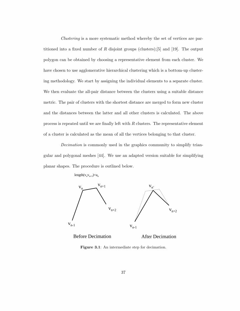
Decimation is commonly used in the graphics community to simplify trian-
gular and polygonal meshes [44]. We use an adapted version suitable for simplifying
planar shapes. The procedure is outlined below.
vnvn+1
vn-1
vn+2
vn-1
vn+2
vn’
length(vnvn+1)=an
Before Decimation After Decimation
Figure 3.1: An intermediate step for decimation.
37

1. Form a priority queue using the edges of the polygon as the key with the maxi-
mum priority assigned to the smallest edge.
2. Choose the EGI vector anun corresponding to the edge with the highest priority.
Let vn and vn+1 be two adjacent vertices which define the above edge.
3. Define a new vertex vn′ given by vn′ = (vn+vn+1)2 and connect it to the adjacent
vertices vn−1 and vn+2 to obtain the edges vn−1vn′ and vn′vn+2. Thus we have
succeeded in decimating one edge.
4. Repeat the above steps until we obtain an R sided polygon.
Thus, by employing the algorithms outlined in this section, we can obtain the
EGI of the polygon using corrupted support and brightness function measurements.
38

Chapter 4
Experimental results
The quality of the reconstructed polygon obtained using the algorithms outlined in
the earlier chapter depend on experimental parameters like noise strength, eccentricity,
scale, viewing set, etc. In this chapter, we use Monte-Carlo simulation results to study
the behavior of our algorithms with respect to changes in these parameters.
We also require a shape comparison metric to quantify the quality of the
reconstructed shapes. A survey of various shape matching metrics can be obtained
in [42]. We employ two commonly used metrics, namely, the Hausdorff distance (δH)
and the Symmetric Difference of Area (S).
The Hausdorff distance between two convex bodies K and L is
δH(K, L) = ‖hK(θ)− hL(θ)‖∞, (4.1)
where hK and hL are the support functions of K and L respectively, and ‖ · ‖∞ is the
infinity norm defined as,
‖x‖∞ = maxi|xi|.
39

The Symmetric Difference of Area between two bodies A and B centered at
the origin can be defined as,
S(A,B) = area((A− B) ∪ (B−A)) (4.2)
In other words it is the area of the non-overlapping regions of the two shapes (for more
details see [15] where a relation between δH and S can also be obtained).
4.1 Sample reconstruction for shape from support-type
functions
Here we present a few sample reconstructions obtained using the algorithms
discussed in the earlier chapter.
4.1.1 Support Functions
Fig. 4.1 demonstrates the reconstructed polygons from support functions ob-
tained by employing all three algorithms, namely, the non-linear algorithm (3.12) and
the two previously proposed algorithms (3.2) and (3.7). All the algorithms were run
under their required assumptions. The underlying shape is a user-defined quadrilat-
eral having barycenter of its vertices at the origin, σ = 0.1, and the support data
is measured from 18 equally spaced viewing directions in the range [0, 2π] (Here and
below, the entire interval, [0, 2π] in this case, is divided into M bins of equal size and
measurement vectors are positioned at the center of each bin.) The quality of shape
reconstruction is compared by calculating the Hausdorff distance between the input
40
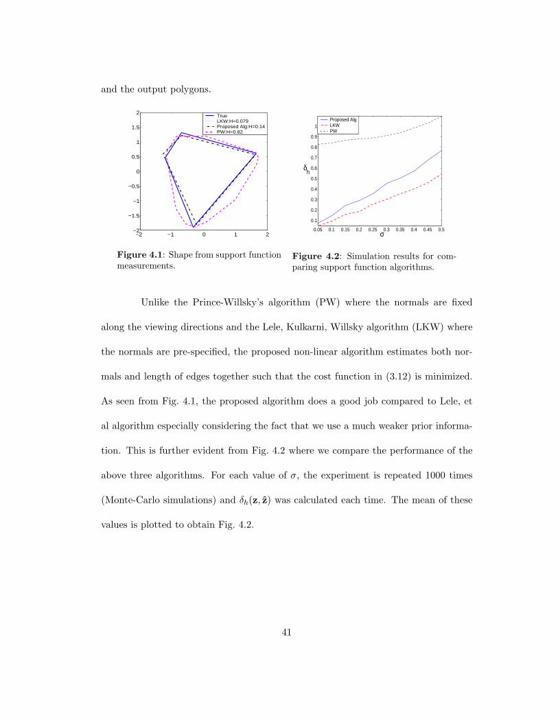
and the output polygons.
−2 −1 0 1 2−2
−1.5
−1
−0.5
0
0.5
1
1.5
2TrueLKW:H=0.079Proposed Alg:H=0.14PW:H=0.82
Figure 4.1: Shape from support functionmeasurements.
0.05 0.1 0.15 0.2 0.25 0.3 0.35 0.4 0.45 0.5
0.1
0.2
0.3
0.4
0.5
0.6
0.7
0.8
0.9
1Proposed AlgLKWPW
δh
σ
Figure 4.2: Simulation results for com-paring support function algorithms.
Unlike the Prince-Willsky’s algorithm (PW) where the normals are fixed
along the viewing directions and the Lele, Kulkarni, Willsky algorithm (LKW) where
the normals are pre-specified, the proposed non-linear algorithm estimates both nor-
mals and length of edges together such that the cost function in (3.12) is minimized.
As seen from Fig. 4.1, the proposed algorithm does a good job compared to Lele, et
al algorithm especially considering the fact that we use a much weaker prior informa-
tion. This is further evident from Fig. 4.2 where we compare the performance of the
above three algorithms. For each value of σ, the experiment is repeated 1000 times
(Monte-Carlo simulations) and δh(z, z) was calculated each time. The mean of these
values is plotted to obtain Fig. 4.2.
41

−1 0 1
−2
−1
0
1
2
OriginalConvex HullReconstructed
Figure 4.3: A non-convex body estimated using brightness functions.
4.1.2 Brightness Functions
The underlying body in Fig. 4.3 is non-convex and the brightness function
values were measured from 36 equally spaced angles in [0, π] and σ = 0.2. The es-
timated shape z obtained using (3.17) is an origin symmetric polygon which closely
approximates the convex-hull of the underlying body as demonstrated in the figure.
−2 −1 0 1 2−2
−1
0
1
2zzhatzout
Figure 4.4: Shape from brightness values
0 0.5 1 1.5 2 2.5 33.4
3.6
3.8
4
4.2
4.4
4.6
4.8
5True (B)Noisy (Bn)Estimated (Bhat)Output (Bout)
θ
Figure 4.5: Brightness values.
The underlying shape in Fig. 4.4 is a user-defined octagon and brightness
42
function were measured from 90 equally spaced viewing directions in [0, π] and σ =
0.05. The estimated polygon z is a 38-sided origin-symmetric polygon obtained using
(3.17). The output polygon zout was obtained from z by pruning the number of sides
down to 16 using decimation. Fig. 4.5 illustrates the true, noisy, estimated and output
brightness function values.
4.2 Effect of experimental parameters
We now analyze the effect of experimental parameters on the quality of re-
construction using Monte-Carlo simulation runs.
4.2.1 Noise strength
The graph in Fig. 4.6 illustrates the behavior of δh(z, z) versus σ. z is a
15-sided regular polygon with eccentricity = 1 where eccentricity ∈ (0, 1] is defined as
the ratio of the minor axis to the major axis of an ellipse inscribing the polygon (a
circle has eccentricity=1). The scale of the polygon (radius of the inscribing polygon)
z is equal to 3 and the brightness function was measured from 36 equally spaced
viewing directions in [0, π]. For each value of σ, the experiment is repeated 1000
times (Monte-Carlo simulations) and δh(z, z) is calculated each time. The mean of
these values (h) is plotted in Fig. 4.6 along with the ±σh vertical error bars (σh is
the standard error of the mean h). We observe that if the noise power increases, the
hausdorff distance between the input and estimated polygon increases and hence the
estimation deteriorates.
43

0 0.2 0.4 0.6 0.8 1 1.2 1.4 1.6 1.8 20
0.1
0.2
0.3
0.4
0.5
0.6
σ
H(z
,zha
t)
Figure 4.6: Effect of noise power
0 0.2 0.4 0.6 0.8 10
0.1
0.2
0.3
0.4
0.5
0.6
0.7
M=18M=36M=90
1/eccentricity
δ h(z
,zhat)
Figure 4.7: Effect of eccentricity
4.2.2 Eccentricity
The graph in Fig. 4.7 illustrates the behavior of our linear algorithm (3.17)
as the eccentricity of the underlying affinely regular polygon changes. Here K = 16,
σ = 0, and scale=1. The figure is composed of three graphs corresponding to three
viewing sets consisting of 18, 36 and 90 equally spaced observation angles respectively.
The error is very small for higher eccentric bodies indicating that it is much easier
to estimate them compared to those with smaller eccentricity. Also note that the
dense viewing set (90 observations) yields better results than the sparse viewing set
(18 measurements) which can be attributed to the simple fact that more number of
observations provide more information thereby implying better estimates.
4.2.3 Scale
The underlying polygon in Fig. 4.8 is a 12-sided regular polygon and the
brightness values were measured from 36 equally spaced viewing directions in [0, π].
The scale of the underlying polygon is varied and the Hausdorff error is calculated
44
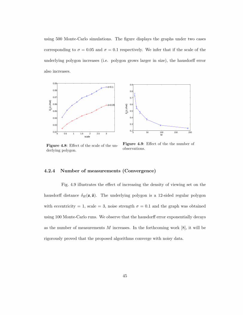
using 500 Monte-Carlo simulations. The figure displays the graphs under two cases
corresponding to σ = 0.05 and σ = 0.1 respectively. We infer that if the scale of the
underlying polygon increases (i.e. polygon grows larger in size), the hausdorff error
also increases.
0 0.5 1 1.5 2 2.5 30.02
0.03
0.04
0.05
0.06
0.07
0.08
0.09
σ=0.1
σ=0.05
scale
δ h(z
,zh
at)
Figure 4.8: Effect of the scale of the un-derlying polygon.
0 50 100 150 2000.2
0.3
0.4
0.5
0.6
0.7
0.8
0.9
M
δ h(z,z
hat)
Figure 4.9: Effect of the the number ofobservations.
4.2.4 Number of measurements (Convergence)
Fig. 4.9 illustrates the effect of increasing the density of viewing set on the
hausdorff distance δH(z, z). The underlying polygon is a 12-sided regular polygon
with eccentricity = 1, scale = 3, noise strength σ = 0.1 and the graph was obtained
using 100 Monte-Carlo runs. We observe that the hausdorff error exponentially decays
as the number of measurements M increases. In the forthcoming work [8], it will be
rigorously proved that the proposed algorithms converge with noisy data.
45
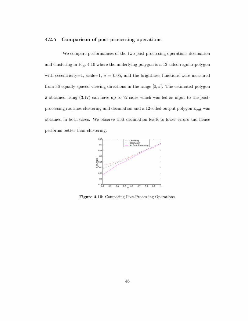
4.2.5 Comparison of post-processing operations
We compare performances of the two post-processing operations decimation
and clustering in Fig. 4.10 where the underlying polygon is a 12-sided regular polygon
with eccentricity=1, scale=1, σ = 0.05, and the brightness functions were measured
from 36 equally spaced viewing directions in the range [0, π]. The estimated polygon
z obtained using (3.17) can have up to 72 sides which was fed as input to the post-
processing routines clustering and decimation and a 12-sided output polygon zout was
obtained in both cases. We observe that decimation leads to lower errors and hence
performs better than clustering.
0.2 0.3 0.4 0.5 0.6 0.7 0.8 0.9 10.05
0.1
0.15
0.2
0.25
0.3
0.35
0.4
0.45
σ
δ H(z
,zou
t)
ClusteringDecimationNo Post−Processing
δ h(z,z
out)
Figure 4.10: Comparing Post-Processing Operations.
46

Chapter 5
Statistical analysis using CRLB
and confidence regions
In this chapter we present statistical analysis of the problem by employing the Cramer-
Rao lower bound analysis and the confidence region visualization technique. Confi-
dence regions quantitate and conveniently display the dependence of the experimental
parameters like eccentricity, noise, viewing set, etc on the quality of the estimated
shape thereby providing a more intuitive and elaborative understanding.
5.1 The (unconstrained) Cramer-Rao lower bound
The Cramer-Rao lower bound (CRLB) is a statistical tool often used in the
performance evaluation of estimation problems. It provides the theoretical lower bound
on the variance of any unbiased estimator; see, for example, [23, pp. 27–35]. Since no
unbiased estimator can have lower variance than the CRLB, it provides a benchmark
for comparison in the performance of an algorithm. Consider an observation vector x
47

given by
x = f(Ψ) + w (5.1)
where Ψ = [ψ1, . . . , ψP ]T is the vector of parameters to be estimated and w is the
noise. The CRLB (see [23, pp. 30–44]) states that the covariance matrix is bounded
below as follows:
Cov(Ψ) ≥ J−1(Ψ). (5.2)
Here Ψ is the vector of estimated parameters and J(Ψ) is a P × P matrix called the
Fisher information matrix (FIM), whose entries are given by the following expression
involving the probability density function (p.d.f.) p(x;Ψ) of the observed data:
J(i, j) = [J(Ψ)]ij = −E
(∂2 ln p(x;Ψ)
∂ψi∂ψj
), (5.3)
for i, j = 1, . . . , P , and where E(.) denotes the expected value.
We first apply this bound to the problem of reconstructing from noisy support
functions modelled by (3.11), with assumptions needed to derive (3.12). Therefore,
this analysis is valid if the underlying polygon has barycenter of vertices at the origin
and the correspondence tm for every viewing direction is known. Recall that the noise
is Gaussian with variance σ2. The observation vector is x = [h(α1), . . . , h(αM )]T and
the parameter vector is Ψ = [a1, . . . , aN , θ1, . . . , θN ]T , so that P = 2N . It follows from
(3.8) that the joint p.d.f. for the support function data is
ph(x;Ψ) =M∏
m=1
1√2πσ2
exp
−1
2σ2
(h(αm)−
N∑
k=1
dtmkak sin(αm − θk)
)2 . (5.4)
48

The FIM will be a 2N × 2N matrix consisting of four N ×N blocks J1, J2, J3, and
J4. Specifically, for i, j = 1, . . . , N , we have
J1(i, j) = J(i, j) = −E
(∂2 ln p(x;Ψ)
∂ai∂aj
)=
1σ2
M∑
m=1
dtmidtmjsm,i sm,j , (5.5)
J2(i, j) = J(i, j + N) = −E
(∂2 ln p(x;Ψ)
∂ai∂θj
)= − aj
σ2
M∑
m=1
dtmidtmjsm,i cm,j , (5.6)
J3(i, j) = J(i + N, j) = −E
(∂2 ln p(x;Ψ)
∂θi∂aj
)= − ai
σ2
M∑
m=1
dtmidtmjsm,j cm,i, (5.7)
and
J4(i, j) = J(i + N, j + N) = −E
(∂2 ln p(x;Ψ)
∂θi∂θj
)=
aiaj
σ2
M∑
m=1
dtmidtmjcm,i cm,j ,
(5.8)
where cm,k = cos(αm−θk) and sm,k = sin(αm−θk). For calculations, see Appendix A.
Thus J is a function of both the EGI vector parameters and the set of measurement
directions.
Next we apply this bound to the problem of reconstructing from noisy bright-
ness functions modelled by (3.13). Here we need to calculate the CRLB for only half
the number of parameters due to the origin symmetry of the reconstruction. The
observation vector x = [b(α1), . . . , b(αM )]T and the reduced space parameter vector is
Ψ = [a1, . . . , aN/2, θ1, . . . , θN/2]T , so that P = N . Using (2.32), (3.13) and under the
Gaussian noise assumption, the joint p.d.f. for the brightness function data is
pb(x;Ψ) =M∏
m=1
1√2πσ2
exp
−1
2σ2
b(αm)−
N/2∑
k=1
ak| cos(αm − θk)|
2 (5.9)
and the FIM is an N × N matrix consisting of four N/2 × N/2 blocks we will again
49

label J1, J2, J3, and J4. Specifically, for i, j = 1, . . . , N/2, we have
J1(i, j) = J(i, j) = −E
(∂2 ln p(x;Ψ)
∂ai∂aj
)=
1σ2
M∑
m=1
|cm,i| |cm,j |, (5.10)
J2(i, j) = J(i, j + N/2) = −E
(∂2 ln p(x;Ψ)
∂ai∂θj
),
=aj
σ2
M∑
m=1
|cm,i| sm,j sgn(cm,j), (5.11)
J3(i, j) = J(i + N/2, j) = −E
(∂2 ln p(x;Ψ)
∂θi∂aj
),
=ai
σ2
M∑
m=1
|cm,j | sm,i sgn(cm,i), (5.12)
and
J4(i, j) = J(i + N/2, j + N/2) = −E
(∂2 ln p(x;Ψ)
∂θi∂θj
)
=aiaj
σ2
M∑
m=1
sm,i sm,j sgn(cm,i) sgn(cm,j),(5.13)
where cm,k = cos(αm−θk), sm,k = sin(αm−θk), and sgn(f) returns +1 or -1 according
to whether f takes positive or negative values, respectively. For calculations, see
Appendix A.
For brightness function measurements, the lower bound on the variance of
the estimated shape parameters for any input polygon can be obtained from (5.2) and
the inverse of the FIM from (5.10)–(5.13). The covariance matrix is an N ×N matrix
and consists of 4 blocks each of size N/2×N/2 as shown in (5.14).
Cov([a1, . . . , aN/2, θ1, . . . , θN/2]T ) =
C1 C2
C3 C4
(5.14)
Using the origin symmetry property of the polygon, we can obtain the co-
50
variance matrix of the complete parameter space [a1, . . . , aN , θ1, . . . , θN ]T from (5.14)
by simple replication as shown in (5.15).
Cov([a1, . . . , aN , θ1, . . . , θN ]T ) =
C1 C1 C2 C2
C1 C1 C2 C2
C3 C3 C4 C4
C3 C3 C4 C4
(5.15)
Thus, the lower bound on the covariance of the EGI parameters estimated using bright-
ness function measurements for a planar body is given by (5.15).
Similarly, for support function measurements, the lower bound on the esti-
mated parameter vector [a1, . . . , aN , θ1, . . . , θN ]T can be calculated from (5.2) and the
inverse of the FIM given by (5.5)–(5.8). However, in this case, the FIM turns out
to be singular with rank (2N − 2), yielding an infinite lower bound. The reason for
this behavior is that the equality constraint (2.9) from Minkowski’s conditions has not
been taken into account. For brightness function measurements, only the inequality
constraint (2.8) comes into play, in view of the formulation in (3.19). Such inequality
constraints induce open subsets in the parameter space without any isolated bound-
aries and so do not affect the CRLB; see [13] for more details. On the other hand,
equality constraints can reduce the dimension of the parameter space and cannot be
ignored in the calculations. The next section addresses this issue.
51

5.2 The constrained Cramer-Rao lower bound
In this section we use the results of Stoica and Ng [40] for a constrained
Cramer-Rao lower bound (CCRLB) analysis with a singular FIM.
Let gi(Ψ) = 0, i = 1, . . . , Q, where Ψ ∈ <P and Q < P , be equality con-
straints defined by continuously differentiable functions, and let g(Ψ) = [g1(Ψ), . . . ,gQ(Ψ)]T
be the corresponding constraint vector. The gradient matrix of g is a Q × P matrix
defined by
G(Ψ) =∂g(Ψ)∂ΨT
,
where G should have full rank. Let U ∈ <P×(P−Q) be an orthogonal matrix in the
null space of G(Ψ). Then
G(Ψ)U = 0.
The analysis in [40] shows that, under the given constraints, the covariance matrix of
the estimated parameters should now satisfy,
Cov(Ψ) ≥ U(UTJU)−1UT . (5.16)
As seen from (5.16), the covariance matrix is obtained by projecting the singular fisher
information matrix onto the constraint subspace.
Minkowski’s condition introduces two equality constraints given by (2.9), and
the gradient matrix of these constraints is the 2× 2N matrix
G(Ψ) =
cos θ1 · · · cos θN −a1 sin θ1 · · · −aN sin θN
sin θ1 · · · sin θN a1 cos θ1 · · · aN cos θN
. (5.17)
52

After carrying out the analysis discussed in this section and using (5.16)
and (5.17), we will be able to obtain the CCRLB for the estimated parameters. To
summarize, the lower bound on the variance of the estimated EGI parameters for
brightness functions and support functions can be obtained using (5.15) and (5.16)
respectively. However, our final aim is to reconstruct the 2-D shape from support-
type function data and not simply to find its EGI. Thus what we really need is to find
bounds with respect to the 2-D shape and not just the parameters. Rather than the
quality of estimates of Ψ, we need a global quality measure of the entire reconstructed
boundary. This can be achieved by developing asymptotic confidence regions around
the true shape, a topic introduced in the next section.
5.3 Confidence Region Analysis
5.3.1 Introduction
Asymptotic global confidence regions are used to analyze and visualize the
performance of 2-dimensional parametric shape estimators. Assuming a maximum
likelihood estimator (MLE) operating in the asymptotic regime, the CRLB for the
shape parameters can be used to define a confidence region around the true boundary
of the shape, as in [43]. Note that the MLE is asymptotically normal, unbiased and
asymptotically attains the CRLB; see [23, pp. 164–167]. We follow [43] below; in our
analysis to develop confidence regions.
Consider a 2-D shape parameterization of the form,
s(t;Ψ) = [sx(t;Ψ), sy(t;Ψ)]T ,
53
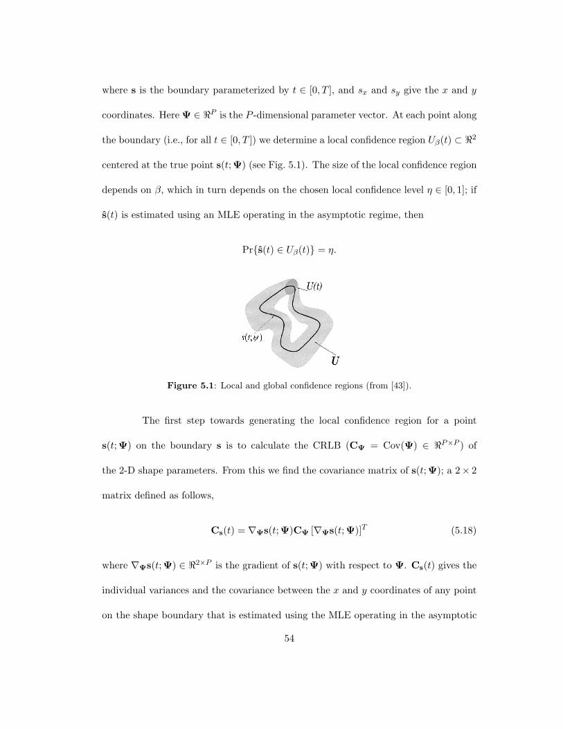
where s is the boundary parameterized by t ∈ [0, T ], and sx and sy give the x and y
coordinates. Here Ψ ∈ <P is the P -dimensional parameter vector. At each point along
the boundary (i.e., for all t ∈ [0, T ]) we determine a local confidence region Uβ(t) ⊂ <2
centered at the true point s(t;Ψ) (see Fig. 5.1). The size of the local confidence region
depends on β, which in turn depends on the chosen local confidence level η ∈ [0, 1]; if
s(t) is estimated using an MLE operating in the asymptotic regime, then
Prs(t) ∈ Uβ(t) = η.
Figure 5.1: Local and global confidence regions (from [43]).
The first step towards generating the local confidence region for a point
s(t;Ψ) on the boundary s is to calculate the CRLB (CΨ = Cov(Ψ) ∈ <P×P ) of
the 2-D shape parameters. From this we find the covariance matrix of s(t;Ψ); a 2× 2
matrix defined as follows,
Cs(t) = ∇Ψs(t;Ψ)CΨ [∇Ψs(t;Ψ)]T (5.18)
where ∇Ψs(t;Ψ) ∈ <2×P is the gradient of s(t;Ψ) with respect to Ψ. Cs(t) gives the
individual variances and the covariance between the x and y coordinates of any point
on the shape boundary that is estimated using the MLE operating in the asymptotic
54
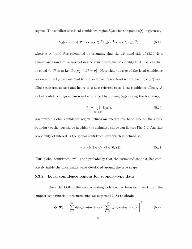
regime. The smallest size local confidence region Uβ(t) for the point s(t) is given as,
Uβ(t) = x ∈ <2 : (x− s(t))TCs(t)−1(x− s(t)) ≤ β2 (5.19)
where β > 0 and β is calculated by assuming that the left-hand side of (5.19) is a
Chi-squared random variable of degree 2 such that the probability that it is less than
or equal to β2 is η; i.e. Prχ22 ≤ β2 = η. Note that the size of the local confidence
region is directly proportional to the local confidence level η. For each t, Uβ(t) is an
ellipse centered at s(t) and hence it is also referred to as local confidence ellipse. A
global confidence region can now be obtained by moving Uβ(t) along the boundary,
Uβ =⋃
t∈[0,T ]
Uβ(t). (5.20)
Asymptotic global confidence region defines an uncertainty band around the entire
boundary of the true shape in which the estimated shape can lie (see Fig. 5.1) Another
probability of interest is the global confidence level which is defined as,
γ = Prs(t) ∈ Uβ, ∀t ∈ [0, T ] (5.21)
Thus global confidence level is the probability that the estimated shape s, lies com-
pletely inside the uncertainty band developed around the true shape.
5.3.2 Local confidence regions for support-type data
Once the EGI of the approximating polygon has been estimated from the
support-type function measurements, we may use (2.18) to obtain
s(t;Ψ) =
[N∑
k=1
dtkak cos(θk + π/2),N∑
k=1
dtkak sin(θk + π/2)
]T
, (5.22)
55

where the discrete values t = 1, . . . , N of t each index a vertex of the polygon. From
this, we find the gradient ∇Ψs(t;Ψ) ∈ <2×2N to be,[
dt1 cos(θ1 + π/2) · · · dtN cos(θN + π/2) −dt1a1 sin(θ1 + π/2 · · · −dtNaN sin(θN + π/2)
dt1 sin(θ1 + π/2) · · · dtN sin(θN + π/2) dt1a1 cos(θ1 + π/2) · · · dtNaN cos(θN + π/2)
].
(5.23)
Using (5.18), (5.19), and (5.23), the asymptotic local confidence ellipses Uβ(t) can be
calculated for t = 1, . . . , N .
In the case of support function measurements, the matrix CΨ in (5.18) is
substituted by the CCRLB given by the right-hand side of (5.16). For brightness
functions measurements, we instead use the CRLB given by the right-hand side of
(5.15). For an N -sided polygon, t varies discretely from 1, . . . , N and therefore we
obtain N local confidence regions each centered at its corresponding true vertex st.
−2 −1 0 1 2−2
−1
0
1
2
x
y
Figure 5.2: Local confidence regions forshape from support function.
−1 0 1
−1
0
1
x
y
Figure 5.3: Local confidence regions forshape from brightness function.
Fig. 5.2 shows the local confidence ellipses for a polygon with N = 7 sides
whose support function is measured at M = 180 equally spaced angles. The noise is
Gaussian with σ = 0.2 and the local confidence level is η=0.73. From (2.28) we know
56
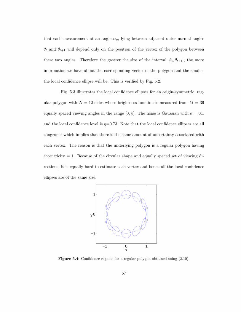
that each measurement at an angle αm lying between adjacent outer normal angles
θt and θt+1 will depend only on the position of the vertex of the polygon between
these two angles. Therefore the greater the size of the interval [θt, θt+1], the more
information we have about the corresponding vertex of the polygon and the smaller
the local confidence ellipse will be. This is verified by Fig. 5.2.
Fig. 5.3 illustrates the local confidence ellipses for an origin-symmetric, reg-
ular polygon with N = 12 sides whose brightness function is measured from M = 36
equally spaced viewing angles in the range [0, π]. The noise is Gaussian with σ = 0.1
and the local confidence level is η=0.73. Note that the local confidence ellipses are all
congruent which implies that there is the same amount of uncertainty associated with
each vertex. The reason is that the underlying polygon is a regular polygon having
eccentricity = 1. Because of the circular shape and equally spaced set of viewing di-
rections, it is equally hard to estimate each vertex and hence all the local confidence
ellipses are of the same size.
−1 0 1
−1
0
1
x
y
Figure 5.4: Confidence regions for a regular polygon obtained using (2.10).
57

If we use the vertex reconstruction method given by (2.10) instead of (2.18)
while defining s(t;Ψ) in (5.22), the local confidence ellipses in Fig. 5.3 instead look like
as shown in Fig. 5.4. Note that the size of the local confidence ellipses increase with
the index t which can be attributed to the unequal error distribution given by (2.26).
The confidence regions in Fig. 5.4 effectively display that (2.10) is a poor method to
obtain shape from EGI.
5.3.3 Effect of experimental parameters on the confidence regions
We now proceed to study the effect of various experimental parameters on
the confidence regions for shape from support type functions.
Noise Power: Increasing the noise corrupting the support-type measurements de-
creases the signal to noise ratio (SNR) and leads to bad estimates. Fig. 5.5 and Fig. 5.6
are obtained using the same shape and parameters as in Fig. 5.2 and Fig. 5.3 respec-
tively, except that the noise strength σ was increased to 0.3 for the support case and
0.2 for the brightness case. We observe that the size of local confidence ellipses has
increased and therefore the associated uncertainty is higher making the estimation
process difficult. An opposite effect is observed if the noise strength is decreased.
Effect of the number of measurements: Increasing the number of measurements
provides more information about the shape which lead to better shape estimation.
Fig. 5.8 is obtained using the same shape and parameters as in Fig. 5.3 except that
the number of brightness function measurements is increased from 36 to 90. We
58

−2 −1 0 1 2−2
−1
0
1
2
x
y
Figure 5.5: Effect of noise power on localconfidence ellipses for support functionsdata.
−1 0 1
−1
0
1
x
y
Figure 5.6: Effect of noise power on lo-cal confidence ellipses for brightness func-tions.
observe that the confidence ellipses have grown smaller in size indicating that the
uncertainty has decreased. Thus we get better shape estimates by increasing the
number of measurements. An opposite effect is observed by decreasing the number of
measurements as evident from Fig. 5.7 which was obtained using 72 equally spaced
viewing directions instead of 180 with the remaining parameters similar to Fig. 5.2.
−2 −1 0 1 2−2
−1
0
1
2
x
y
Figure 5.7: Local confidence ellipses forsupport function with higher number ofmeasurements.
−1 0 1
−1
0
1
x
y
Figure 5.8: Local confidence ellipses forbrightness function with fewer measure-ments.
59

−1 0 1
−1
0
1
x
y
Figure 5.9: Measurement angles sampled from Von-Mises distribution
Randomly drawn viewing set: In Fig. 5.6, the underlying polygon and parameters
are as in Fig. 5.3, but the M = 1000 measurement angles are randomly drawn from the
von Mises distribution V (π/3, 5) (see [34]) with mean π/3 and concentration parameter
κ = 5. The high value of κ leads to a very heavy concentration of measurement angles
near π/3. A brightness function measurement provides the greatest information about
the vertices of the polygon contained in the support lines parallel to the measurement
direction. This explains the very different sizes of the local confidence ellipses in
Fig. 5.6, which are largest at the vertices that lie in support lines parallel to the
relatively few measurement directions orthogonal to π/3.
Effect of eccentricity Fig. 5.10 is obtained using an affinely regular polygon with
N = 8 sides whose support function is measured at M = 72 equally spaced angles,
with σ = 0.1. The local confidence ellipses vary in size, the largest occurring at
vertices 1 and 5 where the “curvature” is smallest. This is compatible with earlier
60

−2 −1 0 1 2−2
−1
0
1
2
x
1 5
4
3
2
6 8
7
y
Figure 5.10: Local confidence regions foran affinely regular polygon with equallyspaced measurement directions.
−2 −1 0 1 2−2
−1
0
1
2
x
1
2
3
4
5
6
7
8
y
Figure 5.11: Local confidence regions foran affinely regular polygon with a betterset of viewing directions.
remarks. If the user has prior information about the eccentricity of the input polygon,
the distribution of the measurement angles can be changed accordingly to compensate.
This is demonstrated in Fig. 5.11, where a total of 72 measurements are made in 12
equally spaced directions each in the intervals [0, π/6), [π/6, 5π/6) and [5π/6, π), and
the 36 antipodal directions. The local confidence ellipse have become more nearly
equal in size.
5.3.4 Global Confidence Region
From the discussion in the previous subsection, we can only develop the local
confidence region for the vertices of the polygon. In this case the global confidence
region Uβ as defined in (5.20) will not give us an uncertainty band around the entire
shape. Moreover, we are not able to find the local confidence region for any point
on the boundary of the polygon; as we are restricted to the vertices. The motivation
behind this sub-section is to enable us to find the confidence region for any point on
61

the shape boundary thereby giving us the global confidence region which will be in
the form of a continuous uncertainty band completely enclosing the true shape as in
Fig. 5.1.
We are restricted to the confidence regions of only the vertices because t in
(5.22) takes on discrete values in the interval [1, N ] with each value of t indexing a
vertex of the polygon. Let us define a shape parameter τ which can take continuous
values in the interval [1, N + 1]. The new shape parameterization s(τ,Ψ) can be
obtained as follows,
s(τ ;Ψ) = (dτe − τ)s(bτc;Ψ) + (τ − bτc)s(dτe;Ψ) (5.24)
where bτc = floor(τ) i.e. rounding τ towards the direction of negative infinity, and
dτe = ceil(τ) i.e. rounding τ towards the direction of positive infinity. Note that τ = 1
and τ = N + 1 refer to the same point on the polygon boundary. Using (5.22) and
substituting t = bτc we get,
s(bτc;Ψ) =
[N∑
k=1
dbτc(k)ak cos(θk + π/2),N∑
k=1
dbτc(k)ak sin(θk + π/2)
](5.25)
Similarly using (5.22) and substituting t = dτe we get,
s(dτe;Ψ) =
[N∑
k=1
ddτe(k)ak cos(θk + π/2),N∑
k=1
ddτe(k)ak sin(θk + π/2)
](5.26)
Finally from (5.24),(5.25) and (5.26) we get,
s(τ ;Ψ) =
[N∑
k=1
qτkak cos(θk + π/2),N∑
k=1
qτkak sin(θk + π/2)
]T
, (5.27)
for 1 ≤ τ ≤ N + 1, where
qτk = (dτe − τ)dbτck + (τ − bτc)ddτek.
62
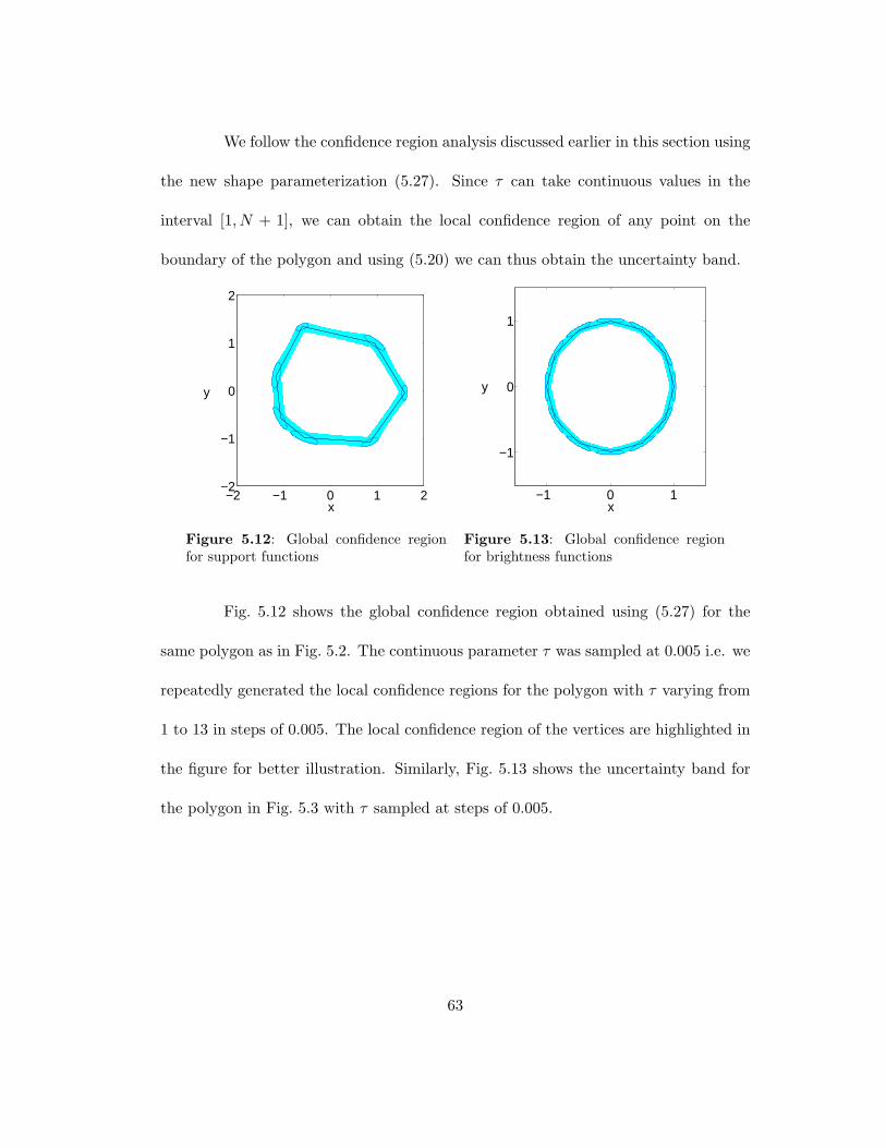
We follow the confidence region analysis discussed earlier in this section using
the new shape parameterization (5.27). Since τ can take continuous values in the
interval [1, N + 1], we can obtain the local confidence region of any point on the
boundary of the polygon and using (5.20) we can thus obtain the uncertainty band.
−2 −1 0 1 2−2
−1
0
1
2
x
y
Figure 5.12: Global confidence regionfor support functions
−1 0 1
−1
0
1
x
y
Figure 5.13: Global confidence regionfor brightness functions
Fig. 5.12 shows the global confidence region obtained using (5.27) for the
same polygon as in Fig. 5.2. The continuous parameter τ was sampled at 0.005 i.e. we
repeatedly generated the local confidence regions for the polygon with τ varying from
1 to 13 in steps of 0.005. The local confidence region of the vertices are highlighted in
the figure for better illustration. Similarly, Fig. 5.13 shows the uncertainty band for
the polygon in Fig. 5.3 with τ sampled at steps of 0.005.
63

Chapter 6
Performance analysis and furtherexperimental results
In this chapter, we use confidence regions to carry out a statistical performance analysis
of our proposed algorithms to find out how close we are to optimal. Later, we also
present some experimental results demonstrating both the sample reconstructions and
the uncertainty regions together.
6.1 Performance Analysis
The optimal algorithm is the MLE operating in the asymptotic regime, since
it is normal, unbiased, and attains the CRLB. Though the algorithms we have consid-
ered above are not necessarily unbiased, their performance can be measured effectively
by comparing them with the MLE operating in the asymptotic regime, using the con-
fidence regions developed earlier for this algorithm. The performance analysis can be
carried out with the aid of both local and global confidence regions as discussed below.
64
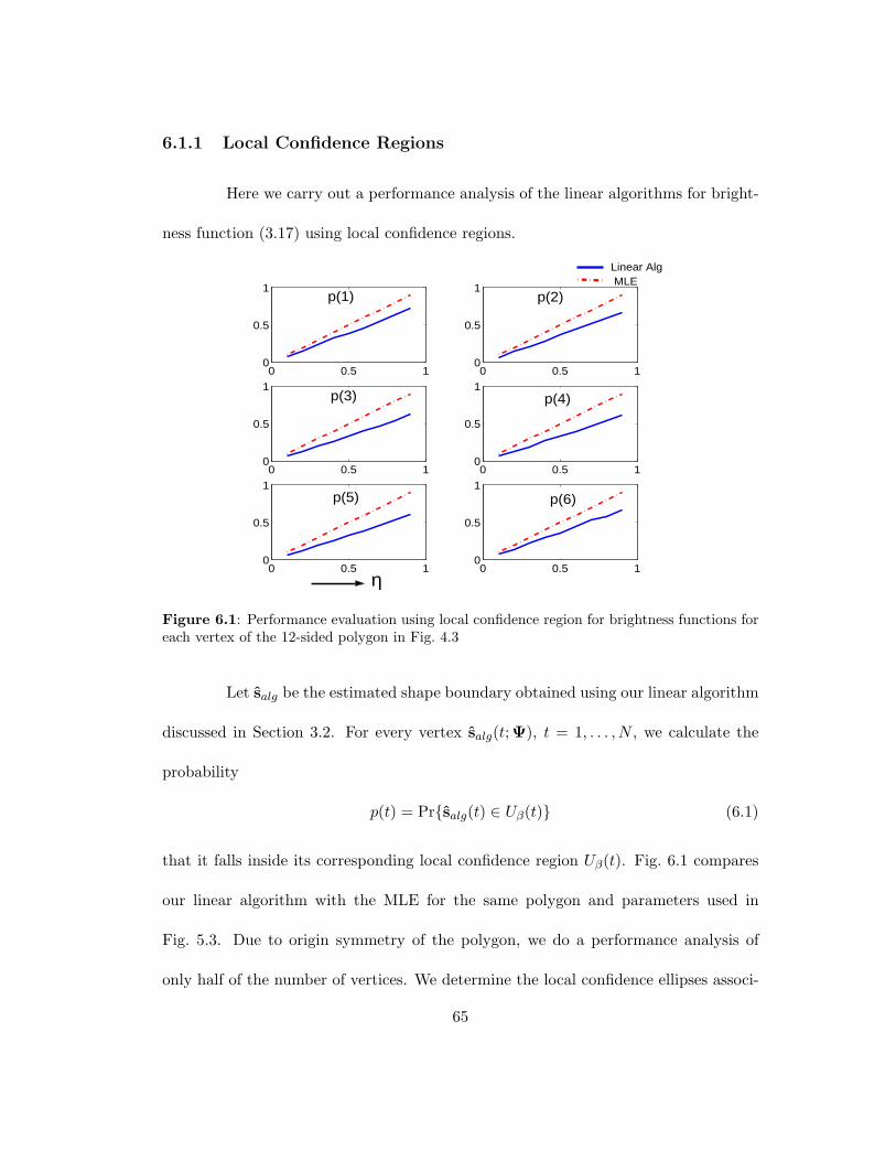
6.1.1 Local Confidence Regions
Here we carry out a performance analysis of the linear algorithms for bright-
ness function (3.17) using local confidence regions.
0 0.5 10
0.5
1
0 0.5 10
0.5
1
0 0.5 10
0.5
1
0 0.5 10
0.5
1
0 0.5 10
0.5
1
0 0.5 10
0.5
1
p(1) p(2)
p(3) p(4)
p(5) p(6)
Linear Alg MLE
η
Figure 6.1: Performance evaluation using local confidence region for brightness functions foreach vertex of the 12-sided polygon in Fig. 4.3
Let salg be the estimated shape boundary obtained using our linear algorithm
discussed in Section 3.2. For every vertex salg(t;Ψ), t = 1, . . . , N , we calculate the
probability
p(t) = Prsalg(t) ∈ Uβ(t) (6.1)
that it falls inside its corresponding local confidence region Uβ(t). Fig. 6.1 compares
our linear algorithm with the MLE for the same polygon and parameters used in
Fig. 5.3. Due to origin symmetry of the polygon, we do a performance analysis of
only half of the number of vertices. We determine the local confidence ellipses associ-
65
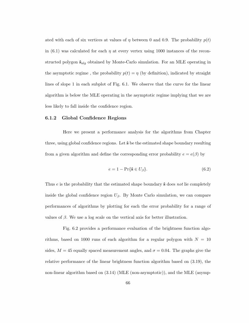
ated with each of six vertices at values of η between 0 and 0.9. The probability p(t)
in (6.1) was calculated for each η at every vertex using 1000 instances of the recon-
structed polygon salg obtained by Monte-Carlo simulation. For an MLE operating in
the asymptotic regime , the probability p(t) = η (by definition), indicated by straight
lines of slope 1 in each subplot of Fig. 6.1. We observe that the curve for the linear
algorithm is below the MLE operating in the asymptotic regime implying that we are
less likely to fall inside the confidence region.
6.1.2 Global Confidence Regions
Here we present a performance analysis for the algorithms from Chapter
three, using global confidence regions. Let s be the estimated shape boundary resulting
from a given algorithm and define the corresponding error probability e = e(β) by
e = 1− Prs ∈ Uβ. (6.2)
Thus e is the probability that the estimated shape boundary s does not lie completely
inside the global confidence region Uβ. By Monte Carlo simulation, we can compare
performances of algorithms by plotting for each the error probability for a range of
values of β. We use a log scale on the vertical axis for better illustration.
Fig. 6.2 provides a performance evaluation of the brightness function algo-
rithms, based on 1000 runs of each algorithm for a regular polygon with N = 10
sides, M = 45 equally spaced measurement angles, and σ = 0.04. The graphs give the
relative performance of the linear brightness function algorithm based on (3.19), the
non-linear algorithm based on (3.14) (MLE (non-asymptotic)), and the MLE (asymp-
66

0.5 1 1.5 2 2.5 3 3.510
−3
10−2
10−1
100
Linear algorithmMLE (non−asymptotic)MLE (asymptotic)
β
e
Figure 6.2: Performance evaluation of brightness function algorithms.
totic). The latter is produced as follows. Since the MLE is asymptotically normal,
unbiased, and attains the CRLB, we first draw an EGI sample from the normal dis-
tribution N(Ψ,CΨ) where the matrix CΨ is is given by the right-hand side of (5.15).
From the EGI sample we obtain the estimated boundary s by (5.22), and the value
of e in (6.2) is estimated from 1000 independent trials of this type. Fig. 6.2 indicates
in particular that the linear brightness function algorithm does a reasonably good job
when compared to the optimal MLE estimator.
−2 −1 0 1 2−2
−1
0
1
2
x
y 0
Figure 6.3: Underlying polygon used forthe analysis in Fig. 6.4.
0.5 1 1.5 2 2.5 3 3.510
−3
10−2
10−1
100
PWLKWMLE (non−asymptotic)MLE (asymptotic)
β
e
Figure 6.4: Performance evaluation ofsupport function algorithms.
67

Fig. 6.4 provides a similar evaluation of the support function algorithms,
based on 1000 runs of each algorithm for a polygon with N = 5 sides, M = 72
equally spaced measurement angles, and σ = 0.1. The underlying polygon has vertices
with barycenter at 0 as shown in Fig. 6.3. The graphs in Fig. 6.4 give the relative
performance of the algorithms of Prince and Willsky (PW), Lele, Kulkarni, and Willsky
(LKW), the non-linear algorithm based on (3.12) (MLE (non-asymptotic)), and the
MLE (asymptotic). However, we stress that the comparison is not really a fair one,
since on the one hand the PW algorithm produces outputs with outer normals in
the measurement directions, and on the other, the LKW algorithm assumes, as prior
knowledge, unknown outer normal angles. In view of this it is hardly surprising that
the PW algorithm performs much worse, and the KLW algorithm much better, than
the MLE algorithms.
6.2 More Experimental Results
Figure 6.5: Shape from support functionmeasurements.
0 1.57 3.14 4.71 6.280.6
0.8
1
1.2
1.4
1.6True NoisyEstimated
α
hK(α)
Figure 6.6: True, noisy, and estimatedsupport function measurements.
Figs. 6.5 and 6.7 illustrate true (solid line) and estimated (dotted line) poly-
68
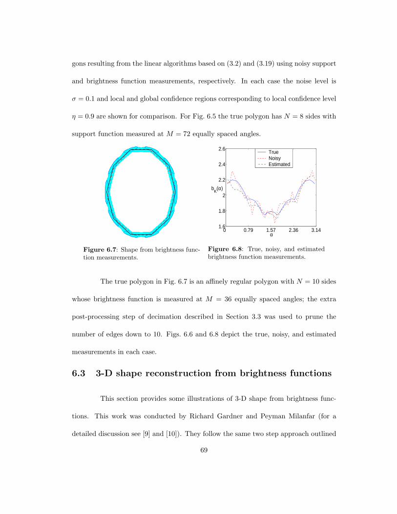
gons resulting from the linear algorithms based on (3.2) and (3.19) using noisy support
and brightness function measurements, respectively. In each case the noise level is
σ = 0.1 and local and global confidence regions corresponding to local confidence level
η = 0.9 are shown for comparison. For Fig. 6.5 the true polygon has N = 8 sides with
support function measured at M = 72 equally spaced angles.
Figure 6.7: Shape from brightness func-tion measurements.
0 0.79 1.57 2.36 3.141.6
1.8
2
2.2
2.4
2.6TrueNoisyEstimated
α
bK(α)
Figure 6.8: True, noisy, and estimatedbrightness function measurements.
The true polygon in Fig. 6.7 is an affinely regular polygon with N = 10 sides
whose brightness function is measured at M = 36 equally spaced angles; the extra
post-processing step of decimation described in Section 3.3 was used to prune the
number of edges down to 10. Figs. 6.6 and 6.8 depict the true, noisy, and estimated
measurements in each case.
6.3 3-D shape reconstruction from brightness functions
This section provides some illustrations of 3-D shape from brightness func-
tions. This work was conducted by Richard Gardner and Peyman Milanfar (for a
detailed discussion see [9] and [10]). They follow the same two step approach outlined
69
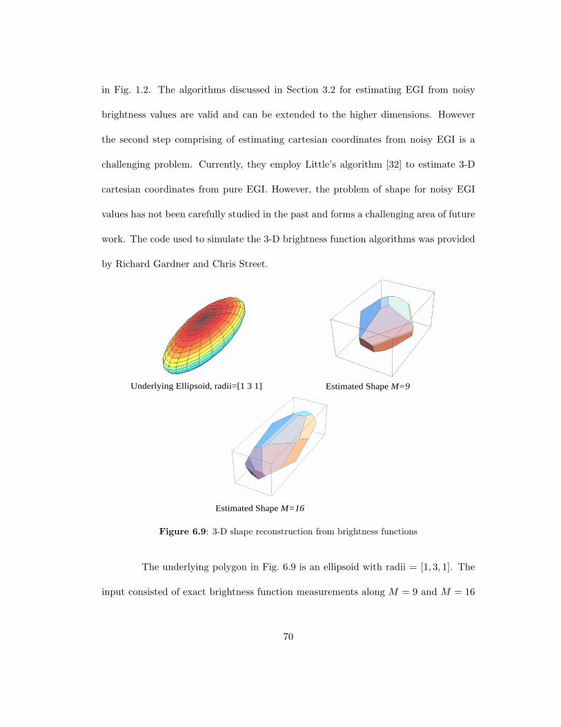
in Fig. 1.2. The algorithms discussed in Section 3.2 for estimating EGI from noisy
brightness values are valid and can be extended to the higher dimensions. However
the second step comprising of estimating cartesian coordinates from noisy EGI is a
challenging problem. Currently, they employ Little’s algorithm [32] to estimate 3-D
cartesian coordinates from pure EGI. However, the problem of shape for noisy EGI
values has not been carefully studied in the past and forms a challenging area of future
work. The code used to simulate the 3-D brightness function algorithms was provided
by Richard Gardner and Chris Street.
Underlying Ellipsoid, radii=[1 3 1] Estimated Shape M=9
Estimated Shape M=16
Figure 6.9: 3-D shape reconstruction from brightness functions
The underlying polygon in Fig. 6.9 is an ellipsoid with radii = [1, 3, 1]. The
input consisted of exact brightness function measurements along M = 9 and M = 16
70
viewing directions corresponding to the spherical polar angles
(2πr
3,πs
3
): r = 0, 1, 2, s = 0, 1, 2
(6.3)
and,(
2πr
4,πs
4
): r = 0, 1, 2, 3, s = 0, 1, 2, 3
(6.4)
respectively. Furthermore, the number of facets of the estimated polygon were reduced
down to 30 using clustering as the post-processing operation. We observe that the
output for M = 16 resembles the underlying polygon more closely than that for
M = 9. Thus, as the number of brightness function measurements increase, the
quality of reconstruction improves.
71

Chapter 7
Conclusions and future work
In this chapter, we introduce a new problem called shape reconstruction from “lightness
functions”. We discuss future directions of research emanating from the current work
and also provide conclusive remarks.
7.1 Lightness Functions
The brightness functions measurements obtained using model (2.31) are inde-
pendent of the illumination of the body; the model does not incorporate the presence
and effects of a light source. Imagine an object with lambertian surface that is so
poorly resolved that its entire image falls on a single pixel at any given time. In
this case, the only available information about the object is the time history of its
tracked pixel intensity. If the object is rotating, then the time history is determined
by two factors, namely the brightness function of the object and the illumination of
the object in the direction in which it is exposed to the camera (see Fig. 7.1 for ex-
ample). The measurement of this time history for an atmosphereless body is what
astronomers refer to as the “lightcurve” of the object (see Fig. 7.2 and [11]) and the
72

problem is to estimate the shape of the object using the weak information provided by
the “lightcurves”. Clearly we need to extend the model in (2.31) to account for such
practical scenarios.
Figure 7.1: Images of a rotating asteroidfrom several viewpoints.
Figure 7.2: Lightcurves (from [11]).
We introduce the “lightness functions” which are defined for objects having
lambertian surface that are illuminated by a light source. The light source is considered
infinitely far away from the object it is illuminating and hence all the rays have a
common direction (directional light source). Sunlight which illuminates astral bodies
is a commonly cited example of a directional light source. The radiance of a lambertian
reflector is the same from all viewing directions. Such a surface follow Lambert’s
Cosine Law which states that the radiance from an element of area of a surface varies
as the cosine of the angle between that direction and the perpendicular to the surface
element.
L(P) = ρ cosλ (7.1)
where, L(P) is the diffused reflectance from the surface, ρ is the effective albedo which
73

is proportional to the intensity of the illuminant and the reflectance properties of the
surface, and λ is the angle between the normal to the surface and the incoming light
ray. Note that the brightness function model in (2.31) can also be written as
b(v) =∫
Sf(u)max(uT v, 0)du (7.2)
Using (7.1) and (7.2) we define the lightness function as,
l(v, w) =∫
Sρ(u)f(u)max(−uT v, 0)max(uT w, 0)du (7.3)
Note that the lightness function is a function of the viewing direction v as
well as the direction of the incoming light ray w. Moreover, unlike the brightness
function, the periodicity interval is 2π. The lightness function is also a weaker form
of data compared to brightness functions. Every point on the object boundary has
to satisfy an additional condition given by the term max(uT w, 0) which checks if the
point is visible or not. Therefore, parts of the object that are not illuminated when
observed from a particular viewing direction do not contribute towards the lightness
function measurement.
Fig. 7.3 shows preliminary results for two cases of shape reconstruction using
lightness function. In both the cases, the underlying polygon is a 15-sided regular
polygon with eccentricity=1. The lightness functions are measured from 30 equally
spaced viewing directions in the range [0, π] and σ = 0. For the sake of simplicity, the
albedo values for all the facets of the polygon are assumed to be equal and a known
value which is set equal to 1. We used the linear least squares approach given in
(3.17) to obtain the estimated polygons. The only difference in the two cases is the
74

direction w of the incoming ray of light as seen from Fig. 7.3. Clearly we can see that
the quality of reconstruction is better if the viewing directions are along the brighter
(more illuminated) parts of the body.
Figure 7.3: Two illustrations of shape reconstruction using Lightness Function
If the albedo value for each facet of the polygon is assumed to be unknown,
the system becomes under-determined; a case which we have not yet studied. A future
direction of work would also consist of developing robust algorithms for shape recon-
struction using corrupted lightness function measurements. This will be of particular
interest to the astronomy community; see [11]. We also need to consider the effect of
having more than one light source illuminating the object. It will be also interesting
to see the confidence regions for shape reconstruction using lightness functions.
75

7.2 Uncertainty Ellipsoids for 3-D
The algorithms for estimating the EGI using brightness functions data can be
easily extended to the 3-D case; see [9] and [10]. However, the problem of estimating
cartesian co-ordinates using noisy EGI values for a 3-D object is a very hard problem
and has not been carefully studied in the past. The difficulty of this problem can
be gauged from the fact that the obvious way to do this in the 2-D case turns out
to be statistically inefficient. In the 3-D case, we are currently using the algorithm
proposed by Little in [32] to obtain cartesian shape representation using pure EGI.
However, we do not know yet if it is statistically efficient and whether it faces the
similar problem of accumulating errors for noisy EGI. Moreover this algorithm uses
non-linear optimization which makes the analysis more challenging. We can also repeat
the confidence region analysis presented in this paper and generate the uncertainty
ellipsoids for each vertex of the polyhedra and furthermore the uncertainty volume
enclosing the underlying polyhedra.
7.3 Conclusion
In this thesis, we presented non-linear and linear algorithms for estimating
a convex shape from finitely many noisy measurements of its support or brightness
function. The shape was parameterized using Extended Gaussian Image and we also
derived a statistically efficient method for obtaining the cartesian coordinates of a
polygon from corrupted EGI values. Focusing on the 2-D case, we carried out a
systematic statistical analysis of these algorithms via computation of the Cramer-Rao
76

lower bound on the estimated parameters. Using this bound, we found local and global
confidence regions for the underlying shape, providing a valuable visual demonstration
of the effect of experimental parameters on the quality of estimated shape. For the
support functions, the CRLB was infinity and hence we use the constrained CRLB
to develop the confidence regions. Finally, we presented a performance analysis of
the linear algorithm for shape from brightness functions that indicates this algorithm
operates reasonably well.
77

Appendix A
Here we present the derivation of the Fisher Information Matrix (FIM) for support
and brightness function measurements.
A.1 FIM calculation for Brightness Functions
In this section, we present the analysis for the case of brightness functions.
The measurement model for brightness function measurements of a planar convex
body is,
b(αm) =12
N∑
k=1
ak| cos(αm − θk)|+ n(αm)
where, m = 1, . . . , M and M = total number of observations.
N = total number of edges of the polygon.
αm = mth viewing direction
θk = Normal to the kth side of the polygon
ak = Length of the kth side of the polygon
b(αm) = brightness function measurement along the viewing direction αm
n(αm) = Noise corrupting the brightness function measurement along the direction
αm (assumed to be White Gaussian Noise with zero mean and variance σ2).
78

If the underlying body is origin symmetric, the joint PDF of the observed data can be
obtained from (5.9) as follows,
pb(x;Ψ) =
M∏m=1
1√2πσ2
exp
− 1
2σ2
(b(αm)−
N/2∑k=1
ak| cos(αm − θk)|)2
where the x = [b(α1), . . . , b(αM )]T and Ψ = [a1, . . . , aN/2, θ1, . . . , θN/2]T .
Therefore, the log-likelihood function for the brightness data is given as,
ln pb(x;Ψ) = −M
2ln(2πσ2)− 1
2σ2
M∑m=1
(b(αm)−
N/2∑k=1
ak| cos(αm − θk)|)2
(A.1)
To calculate J1(i, j)
J1(i, j) = −E
(∂2 ln pb(x;Ψ)
∂ai∂aj
)for i, j = 1, . . . , N/2 (A.2)
Differentiating the log-likelihood function (A.1) wrt the parameter ai we get,
∂ ln pb(x;Ψ)
∂ai= − 1
2σ2
M∑m=1
[2
(b(αm)−
N/2∑k=1
ak| cos(αm − θk)|)
∂
∂ai
(−
N/2∑k=1
ak| cos(αm − θk)|)]
=1
σ2
M∑m=1
[(b(αm)−
N/2∑k=1
ak| cos(αm − θk)|)| cos(αm − θi)|
](A.3)
Differentiating (A.3) wrt the parameter aj we get,
∂2 ln pb(x;Ψ)
∂ai∂aj= − 1
σ2
M∑m=1
(| cos(αm − θi)|| cos(αm − θj)|) (A.4)
Therefore, from (A.2) and (A.4) we obtain,
J1(i, j) =1
σ2
M∑m=1
(| cos(αm − θi)|| cos(αm − θj)|)
To calculate J2(i, j) and J3(i, j)
J3(i, j) = J2(j, i) = −E
(∂2 ln pb(x;Ψ)
∂θi∂aj
)for i, j = 1, . . . , N/2
79
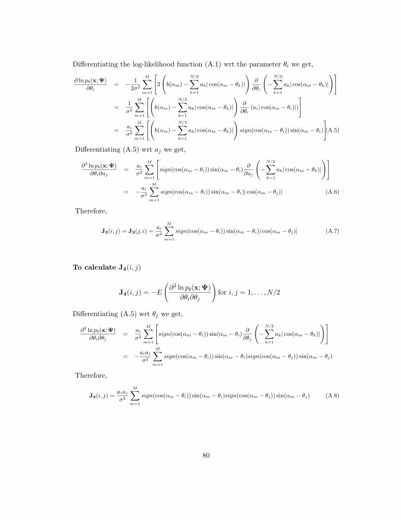
Differentiating the log-likelihood function (A.1) wrt the parameter θi we get,
∂ ln pb(x;Ψ)
∂θi= − 1
2σ2
M∑m=1
[2
(b(αm)−
N/2∑k=1
ak| cos(αm − θk)|)
∂
∂θi
(−
N/2∑k=1
ak| cos(αm − θk)|)]
=1
σ2
M∑m=1
[(b(αm)−
N/2∑k=1
ak| cos(αm − θk)|)
∂
∂θi(ai| cos(αm − θi)|)
]
=ai
σ2
M∑m=1
[(b(αm)−
N/2∑k=1
ak| cos(αm − θk)|)
sign(cos(αm − θi)) sin(αm − θi)
](A.5)
Differentiating (A.5) wrt aj we get,
∂2 ln pb(x;Ψ)
∂θi∂aj=
ai
σ2
M∑m=1
[sign(cos(αm − θi)) sin(αm − θi)
∂
∂aj
(−
N/2∑k=1
ak| cos(αm − θk)|)]
= − ai
σ2
M∑m=1
sign(cos(αm − θi)) sin(αm − θi)| cos(αm − θj)| (A.6)
Therefore,
J3(i, j) = J2(j, i) =ai
σ2
M∑m=1
sign(cos(αm − θi)) sin(αm − θi)| cos(αm − θj)| (A.7)
To calculate J4(i, j)
J4(i, j) = −E
(∂2 ln pb(x;Ψ)
∂θi∂θj
)for i, j = 1, . . . , N/2
Differentiating (A.5) wrt θj we get,
∂2 ln pb(x;Ψ)
∂θi∂θj=
ai
σ2
M∑m=1
[sign(cos(αm − θi)) sin(αm − θi)
∂
∂θj
(−
N/2∑k=1
ak| cos(αm − θk)|)]
= −aiaj
σ2
M∑m=1
sign(cos(αm − θi)) sin(αm − θi)sign(cos(αm − θj)) sin(αm − θj)
Therefore,
J4(i, j) =aiaj
σ2
M∑m=1
sign(cos(αm − θi)) sin(αm − θi)sign(cos(αm − θj)) sin(αm − θj) (A.8)
80

A.2 FIM calculation for Support Functions
In this section, we present the derivation of the Fisher Information Matrix
for support function data. The measurement model for support function data of a
polygon having barycenter of the vertices at the origin is,
y(αm) =N∑
k=1
dtmkak sin(αm − θk) + n(αm),
where the symbols have the same meaning as in Section A.1
Therefore, the joint PDF of the measured support data is given as,
ph(y;Ψ) =
M∏m=1
1√2πσ2
exp
[−1
2σ2
(y(αm)−
N∑k=1
dtmkak sin(αm − θk)
)2], (A.9)
where the y = [y(α1), . . . , y(αm)]T and Ψ = [a1, . . . , aN , θ1, . . . , θN ]T . From (A.9),
the log-likelihood function for the support data is,
lnph(y;Ψ) = −M
2ln(2πσ2)− 1
2σ2
M∑m=1
(y(αm)−
N∑k=1
dtmkak sin(αm − θk)
)2
(A.10)
To calculate J1(i, j)
J1(i, j) = −E
(∂2 ln p(y;Ψ)
∂ai∂aj
)for i, j = 1, . . . , N
Differentiating the log-likelihood function (A.10) wrt ai we obtain,
∂ ln ph(y;Ψ)
∂ai= − 1
2σ2
M∑m=1
[2
(y(αm)−
N∑k=1
dtmkak sin(αm − θk)
)∂
∂ai
(−
N∑k=1
dtmkak sin(αm − θk)
)]
=1
σ2
M∑m=1
[(y(αm)−
N∑k=1
dtmkak sin(αm − θk)
)dtmi sin(αm − θi)
](A.11)
Differentiating the above equation wrt aj we get,
∂2 ln ph(y;Ψ)
∂ai∂aj= − 1
σ2
M∑m=1
dtmidtmj sin(αm − θi) sin(αm − θj) (A.12)
81

Therefore, from (A.12),
J1(i, j) =1
σ2
M∑m=1
dtmidtmj sin(αm − θi) sin(αm − θj) (A.13)
To calculate J2(i, j) and J3(i, j)
J3(i, j) = J2(j, i) = −E
(∂2 ln p(y;Ψ)
∂θi∂aj
)for i, j = 1, . . . , N
Differentiating the log-likelihood function (A.10) wrt θi we obtain,
∂ ln ph(y;Ψ)
∂θi= − 1
2σ2
M∑m=1
[2
(y(αm)−
N∑k=1
dtmkak sin(αm − θk)
)∂
∂θi
(−
N∑k=1
dtmkak sin(αm − θk)
)]
= − ai
σ2
M∑m=1
[(y(αm)−
N∑k=1
dtmkak sin(αm − θk)
)dtmi cos(αm − θi)
](A.14)
Differentiating the above equation wrt aj we get,
∂2 ln ph(y;Ψ)
∂θi∂aj=
ai
σ2
M∑m=1
dtmidtmj sin(αm − θj) cos(αm − θi) (A.15)
Therefore,
J3(i, j) = J2(j, i) = − ai
σ2
M∑m=1
dtmidtmj sin(αm − θj) cos(αm − θi) (A.16)
To calculate J4(i, j)
J4(i, j) = −E
(∂2 ln p(y;Ψ)
∂θi∂θj
)for i, j = 1, . . . , N
Differentiating (A.14) wrt θj we get,
∂2 ln ph(y;Ψ)
∂θi∂θj= −aiaj
σ2
M∑m=1
dtmidtmj cos(αm − θi) cos(αm − θj) (A.17)
Therefore,
J4(i, j) =aiaj
σ2
M∑m=1
dtmidtmj cos(αm − θi) cos(αm − θj) (A.18)
82

Bibliography
[1] N. Ahuja and J. Veenstra, Generating octrees from object silhouettes in ortho-graphic views, IEEE Transactions on Pattern Analysis and Machine Intelligence11 (1989), no. 2, 137–149.
[2] Andrea Bottino, Luc Jaulin, and Aldo Laurentini, Finding feasible parametersets for shape from silhouettes with unknown position of the viewpoints, IEEETransactions on Pattern Analsyis and Machine Intelligence (2003).
[3] S. Campi, A. Colesanti, and P. Gronchi, Convex bodies with extremal volumes hav-ing prescribed brightness in finitely many directions, Geom. Dedicata 57 (1995),121–133.
[4] P. J. Davis, Circulant matrices, Willey Interscience, 1979.
[5] R. O. Duda and P. E. Hart, Pattern classification and scene analysis, Wiley-Interscience, 1973.
[6] N. I. Fisher, P. Hall, B. Turlach, and G. S. Watson, On the estimation of aconvex set from noisy data on its support function, Journal of American StatisticalAssociation 92 (1997), no. 437, 84–91.
[7] R. J. Gardner, Geometric tomography, Cambridge University Press, 1995.
[8] R. J. Gardner, M. Kiderlen, and P. Milanfar, Convergence of algorithms for re-construction from noisy support and brightness functions, Tech. report, (in prepa-ration), 2003.
[9] R. J. Gardner and P. Milanfar, Shape reconstruction from brightness functions,Proceedings of the SPIE Conference on Advanced Signal Proccessing Algorithms,Architecture, and Implementations X (2001), 234–245.
[10] R. J. Gardner and P. Milanfar, Reconstruction of convex bodies from brightnessfunctions, Discrete and Computational Geometry 29 (2003), 279–303.
83
[11] L. Giacomini, Asteroids shapes and rotation: what is a lightcurve?,http://spaceguard.ias.rm.cnr.it/tumblingstone/issues/special-palermo/lightcurve.htm.
[12] G. H. Golub and V. Pereyra, The differentiation of pseudo-inverses and nonlin-ear least squares problems whose variables separate, SIAM Journal of NumericalAnalysis 10 (1973), 413–432.
[13] J. D. Gorman and A. O. Hero, Lower bounds for parametric estimation withconstraints, IEEE Transactions on Imformation Theory 26 (1990), no. 6, 1285–1301.
[14] J. Gregor and F. R. Rannou, Three-dimensional support function estimation andapplication for projection magnetic resonance imaging, International Journal ofImaging System Technology 12 (2002), 43–50.
[15] H. Groemer, On the symmetric difference metric for convex bodies, Contributionsto Algebra and Geometry 41 (2000), no. 1, 107–114.
[16] P. Hall and B. Turlach, On the estimation of a convex set with corners, IEEETransactions on Pattern Analysis and Machine Intelligence 21 (1999), no. 3, 225–234.
[17] G. T. Hermann, Image reconstruction from projections, Academic Press, NewYork, 1980.
[18] B. K. P. Horn, Robot Vision, The MIT Press and McGraw-Hill Book Company,1986.
[19] V. Hosel and S. Walcher, Clustering techniques: A brief survey, Tech. report,Institute of Biomathematics and Biometry, 2001.
[20] M. Ikehata and T. Ohe, A numerical method for finding the convex hull of polyg-onal cavities using the enclosure method, Inverse Problems 18 (2002), 111–124.
[21] A. Kak and M. Slaney, Principles of computerized tomographic imaging, SIAM,IEEE Press, 2001.
[22] W. C. Karl, S. R. Kulkarni, G. V. Verghese, and A. S. Willsky, Local tests forconsistency of support hyperplane data, Journal of Mathematical Imaging andVision 6 (1995), 249–269.
[23] S. Kay, Fundamentals of statistical signal processing - volume II, Prentice-Hall,Englewood Cliffs, 1993.
84
[24] M. Kiderlen, Non-parameteric estimation of the directional distribution of sta-tionary line and fibre processes, Adv. Appl. prob. 33 (2001), 6–24.
[25] L. Lamberg, On the minkowski problem and the lightcurve operator, Ann. Acad.Sci. Fennicae, Math. Diss. 87 (1993).
[26] A. Laurentini, The visual hull concept for silhouette-based image understanding,IEEE Transactions on Pattern Analysis and Machine Intelligence 16 (1994), no. 2,150–162.
[27] A. S. Lele, S. R. Kulkarni, and A. S. Willsky, Convex polygon estimation fromsupport line measurements and applications to target reconstruction from laserradar data, Journal of Optical Society America 9 (1992), 1693–1714.
[28] J. Lemordant, P. D. Tao, and H. Zouaki, Modelisation et optimisation numeriquepour la reconstruction d’un polyedre a partir de son image gaussienne generalisee,,RAIRO Model. Math. Anal. Numer. 27 (1993), 349–374.
[29] S. Y. R. Li, Reconstruction of polygons from projections, Information ProcessingLetters 28, 235–240.
[30] M. Lindenbaum and A. Bruckstein, Reconstructing a convex polygon from binaryperspective projections, Pattern Recognition 23 (1990), no. 12, 1343–1350.
[31] M. Lindenbaum and A. Bruckstein, Blind approximation of planar convex sets,IEEE Transaction on Robotics and Automation 10 (1994), no. 4, 517–529.
[32] J. J. Little, An iterative method for reconstructing convex polyhedra from extendedgaussian images, Proceedings AAAI National Conference on Artificial Intelligence(1983), 247–250.
[33] E. Mammen, J. S. Marron, B. A. Turlach, and M. P. Wand, A general projectionframework for constrained smoothing, Statistical Sciences 16 (2001), no. 3, 232–248.
[34] K. V. Mardia and P. E. Jupp, Directional statistics, Willey, 2001.
[35] W. N. Martin and J. K. Agarwal, Volumetric description of objects from multipleviews, IEEE Transactions on Pattern Analysis and Machine Intelligence 5 (1983),150–158.
[36] J. L. Prince, Geometric model-based estimation from projections, Ph.D. thesis,Massachusetts Institute of Technology, 1988.
[37] J. L. Prince and A. S. Willsky, Estimating convex sets from noisy support line
85

measurements, IEEE Transactions on Pattern Analysis and Machine Intelligence12 (1990), no. 4, 377–389.
[38] A. S. Rao and K. Y. Goldberg, Shape from diameter: Recognizing polygonal partswith a parallel-jaw gripper, International Journal of Robotics Research 13 (1994),no. 1, 16–37.
[39] R. Schneider, Convex bodies: The brunn-minkowski theory, Cambridge UniversityPress, 1993.
[40] P. Stoica and B. C. Ng, On the cramer-rao bound under parametric constraints,IEEE Signal Processing Letters 5 (1998), no. 7, 177–179.
[41] M. A. Sumbatyan and E. A. Troyan, Reconstruction of the shape of a convexdefect from a scattered wave field in the ray approximation, Journal of AppliedMathematics and Mechanics 56 (1992), 464–468.
[42] E. C. Veltkamp, Shape matching: similarity measures and algorithms, Proceedingsof the International Conference on Shape Modelling and Applications (2001), 188–197.
[43] J. C. Ye, Y. Bresler, and P. Moulin, Asymptotic global confidence regions in para-metric shape estimation problems, IEEE Transactions on Information Theory 46(2000), no. 5, 1881–1895.
[44] Pan Zhingeng, Zhou Kun, and Shi Jiaoying, A new mesh simplification algo-rithm based on triangle collapses, Journal of Computer Science and Technology16 (2001), no. 1, 57–63.
86
Top Related