


Languages
Pages
Legal


1
Recent Developments in Unit Root Tests and
Historical Crop Yields
Hector O. Zapata, David I. Maradiaga, Aude L. Pujula Professor and Research Assistants
Department of Agricultural Economics & Agribusiness LSU Agricultural Center 101 Ag Admin Bldg
Baton Rouge, LA 70803 Phone: (225) 578‐2766
Email: [email protected]
Michael R. Dicks Professor
Oklahoma State University 314 AgHall,
Stillwater, OK74078 Phone: (405) 744‐6163
Email: [email protected]
Selected Paper prepared for presentation at the Agricultural & Applied Economics Association’s 2011 AAEA & NAREA Joint Annual Meeting, Pittsburgh, Pennsylvania, July 2426, 2011.
Copyright 2011 by Zapata, Maradiaga, Pujula, and Dicks. All rights reserved. Readers may make verbatim copies of this document for noncommercial purposes by any means, provided that this copyright appears on all such copies.
2
Recent Developments in Unit Root Tests and
Historical Crop Yields
Abstract This study conducts an investigation on the application of classical unit‐root tests using parametric tests (the augmented Dickey‐Fuller, 1979 – ADF), and nonparametric tests (Phillips and Perron, 1988—PP) to corn and soybean yields in the Delta states using county‐level data from 1961 to 2009. The main concern of the paper is to assess what would be drawn about nonstationarity in crop yields using these tests versus using modified versions of these tests (Ng and Perron, 2001) that are assumed to solve size and power problems associated with the ADF and PP tests. The investigation focuses on methodological aspects of the classical tests, uncovers the nature of filtered yields often needed prior to density estimation, sheds light on the effect of lag truncation and provides guidance for future work. It is found that the complexity in yield behavior is such that at very small samples (40 observations or less), results can lead to ambiguous findings in larger samples (49 observations). This sample size analysis with county‐level yield data uncovers that negative moving average effects are present and help explain certain ambiguous findings. As a by‐product, this paper contains a condensed review of literature on unit‐roots that may prove useful in applied research.
Key Words: Crop yields, nonstationarity, unit‐roots, density estimation.

3
Recent Developments in Unit Root Tests and Historical Crop Yields
The large but inconclusive literature on crop yield distributions has been recently
summarized and empirically revisited by a number of researchers (e.g., Harri et al. ,2008)
using a variety of yield models for several thousand data series at the county level for U.S.
crops. One salient finding in these papers is the limited support for stochastic trends in
yields. The main issue driving this type of research has to do with the appropriate
specification of crop yield distributions which are essential in risk management in
agriculture. Clearly, if crop yields were nicely behaved (independent, random, and
normal), specifying the distribution function would be trivial and probability estimates
would be easy to obtain. In practice, however, yields must be filtered (transformed) prior
to identifying a distribution function, and the question of how to best do this remains an
open one. When using historical crop yields, it is well documented that yields can behave
as either deterministic (e.g., linear trend) or stochastic (e.g., unit‐root). Harri et al., for
example, find limited support for stochastic trends in yields..
The extensive literature on this subject has acknowledged the usefulness of the ADF
and PP tests in determining the most adequate functional form to describe technological
change in yield data. Also, the temporal dependence, heterogeneity, and the finite sample
equivalence between a trend‐stationary process and an ARIMA(0,1,1) with a negative MA
coefficient close to the unit‐circle has led some to argue that the standard PP test may be a
better choice. Recent developments in unit‐root tests solve the poor size and power

4
performance of the standard ADF and PP tests and provide new modified tests. Although
modifications to the standard ADF and PP tests have been published in the econometrics
literature over the past decade, it is not until recently that modifications with improved
size and power have been refined, and this may explain the slow adoption of these tests in
applied research. The modification deals with important empirical omissions in the use of
unit‐root tests that should prove useful in a wide variety of applications. First,
modifications to statistical selection criteria used in the identification of lag‐length (e.g.,
using MAIC rather than AIC‐‐ Ng and Perron, 2001; Perron and Qu, 2007) suggest that lag‐
length selection using standard criteria such as the AIC tends to be too small in the
presence of moving average processes with large negative roots. Second, recent work has
shown that the modified tests can have global power problems because of the dependence
on the unit‐root hypothesis; therefore, the estimation of the unit‐root must be decoupled
from that of the long run variance of the process for the tests to have good size properties
when the long‐run variance is estimated using an autoregressive spectral density
estimator. These recent developments are relevant to risk analyses with crop yields
because they accommodate frequently reported regularities in crop yields such as serial
correlation, deterministic components, and non‐Gaussian behavior. This paper applies
these recent developments to county‐level historical crop yields for corn and soybeans in
the Mississippi River Delta Region (Texas, Louisiana, Mississippi, Arkansas, and Missouri)
using county‐crop yields with at least 20 observations to 2009 (a total of 302 counties).
The impact on yield probability estimates from the application of existing procedures and
the new methods are calculated.

5
Literature on Unit Roots
Dickey and Fuller (1979) and Said and Dickey (1984) are perhaps the two most
influential papers on tests for unit roots (DF tests). Of interest is testing the null hypothesis
that the coefficient on the one‐period lagged term of the dependent variable being tested
for unit‐roots equals one versus the alternative that this coefficient is less than one (a
stationary alternative hypothesis). These tests found wide applicability in economics
research and are now standard tools in most econometrics software packages. Because the
DF tests often require the estimation of an autoregression with one or more lags on the
first‐differences of the dependent variable, a statistical model selection criteria is used to
determine the lag length; the DF test calculated from this autoregression is referred to as
the Augmented Dickey‐Fuller (ADF) test. Phillips and Perron (1988) developed a
nonparametric alternative to the ADF tests (PP tests) that found similar wide applicability.
The ADF and PP tests can be specified under three basic models, which can be
specified as:
This is a regression of first‐differences in on a constant term , a linear trend
, a lagged yields and lagged differences of yields. If there are no deterministic
components in the series, then the first two terms are omitted generating a third model
without a constant and without a trend. Some econometric packages (e.g., SHAZAM) report
test statistics for those three models. While it is well known that a t‐type statistic can be

6
used to test for a unit‐root, it appears less well known (or less often used) that Phillips
(1987), and Phillips and Perron suggested a testing strategy for unit‐roots that should first
decipher whether the series in question is trend deterministic (e.g., represented by a
simple linear trend) versus trend stochastic (e.g. unit‐root). Such a test would require
testing a joint hypothesis that the γ and α2 parameters in equation (1) equal zero, and of
course, this is a classical F‐test. Phillips and Perron recommend using this test prior to
proceeding with other tests.
While an extensive review of the literature on unit‐roots for applied researchers
may prove beneficial, we only provide a brief list of the works (in addition to the papers
cited in the previous section) that reflect the main historical progression in testing for unit‐
roots. Schwert (1989) and Perron and Ng (1996) provided Monte Carlo evidence
suggesting that when the moving‐average polynomial of the first‐differenced series has a
large negative root, many tests have size problems, resulting in over‐rejection of the unit‐
root hypothesis. Similarly, the low power of these tests in the presence of an
autoregressive coefficient close to but less than one was noted early (e.g. DeJong et al.,
(1992)). Using a proposition in Stock (1990), Ng and Perron (1996) introduced a class of
modified unit‐root tests with better power (more robust to size distortions in the presence
of negative serial correlation). Later on, Ng and Perron (2001) applied local GLS
detrending (Dufour and King (1991); Elliot, Rothenberg, and Stock (1996)) to the modified
tests to obtain gains in size and power when the modified tests are estimated using an
autoregressive spectral density estimator at frequency zero. These findings also showed
that appropriate selection of the truncation lag was crucial, an issue also studied by others
(e.g. Ng and Perron (1995), and Lopez (1997)) who showed via simulation experiments

7
that there is a strong association between the identified lag‐length and the size and power
of the tests. Ng and Perron (2001) introduced a modified AIC (referred to as MAIC) to
resolve the lag‐length truncation problem (Haldrup and Jasson (2006) provide an excellent
survey of these developments). A few years later, Perron and Qu (2007) discovered that a
simple modification to the lag‐length truncation in Ng and Perron (2001) using OLS (rather
than GLS detrending in selecting the MAIC truncation) would result in tests having an exact
size. All these developments (and an R routine to estimate the tests) can be found in Lupi
(2009).
Unitroots in Crop Yields
Probability density estimation is a recurrent field of research in agricultural
economics. It is of particular interest in risk assessment and has been applied to crop yields
since the fifties. Foote and Bean (1951) followed by Day (1965) were the first to discuss the
issue of non‐normality in crop yield distributions. Their pioneer works laid the foundation
to a vast statistical quest on the subject. Gallagher (1986 and 1987), for example, used a
Gamma distribution to estimate corn and soybean yield density functions and found
evidence of negative skewness, thus suggesting that yields are non‐normally distributed.
Nelson and Preckel (1989) opted for a beta distribution to estimate corn yield distributions
conditional on fertilizer application. According to the authors, the beta distribution has the
advantage of being flexible as it captures the three moments of a probability distribution.
Taylor (1990) brought for the first time the use of the multivariate non‐normal probability
density function that can work under small samples. Taylor found both univariate and
multivariate densities for corn, soybeans and wheat to be negatively skewed. Taylor’s work

8
was the motivation for other multivariate studies such as Ramirez (1997) who also
reported negative skewness. Moss and Shonkwiler (1993) estimated an inverse hyperbolic
sine transformation to model corn yields and found negative skewness. Goodwin and Ker
(1998) were the first to apply non‐parametric techniques to crop yield distributions. Ker
and Goodwin (2000) reexamined Goodwin and Ker’s (1998) methodology and found
significant efficiency gains in estimating conditional yield densities via the empirical Bayes
nonparametric kernel density estimator. In view of the diversity of distributions, Nelson
(1990) attempted to show the impact of the distribution choice on probability estimates
comparing normal and gamma distributions. Other authors have also tried to compare
alternative distributions based on their performance such as Turvey and Zhao (1999),
Norwood et al. (2004) and Sherrick et al. (2004). This list of works is far from exhaustive
but illustrates the array of statistical interest in finding adequate specifications of yield
densities.
The choice of the distribution is not the only matter of disagreement. Indeed, the presence
of trends in crop yields, either deterministic (e.g., linear trend) or stochastic (e.g., unit‐
root), has been largely questioned. In the early literature, levels were used to estimate crop
yield density functions. Foote and Bean (1951) were the first to notice the trending
behavior of corn yields and that the data generation process (DGP) of the latter was most
likely to be non‐random. Likewise, Day (1965) insisted on the importance of understanding
stochastic properties of crop yields in risk assessments. After WWII, with the technological
changes that occurred in agriculture in the U.S. as well as in Europe, the upward trend in
crop yields became unquestionable. Therefore, researchers started to model this behavior
by fitting a linear trend to crop yield data prior to density estimation (e.g., Gallagher, 1986

9
and 1987 and Turvey and Zhao, 1999). Researchers rapidly realized that the impact of
technology as well as major severe climatic events was not so easy to model. Overcoming
these drawbacks, Zapata and Rambaldi (1989) and then, Kaylen and Koroma (1991)
considered stochastic trends in crop yield density estimation for the first time. Similar
works are those of Moss and Shonkwiler (1993) who allowed stochastic trends in crop
yield series using nested models. Goodwin and Ker (1998) carefully determined the DGP
and found that an ARIMA (0,1,2) and thus stochastic processes, best represented crop yield
series. In consequence, they have applied first differencing to the data before generating
non‐parametric (Kernel) crop yield density functions. The use of ARIMA filters in crop yield
distribution estimation is rooted in some traditional works (e.g. Bessler, 1980, p.666). As
suggested by time‐series theory and simulated in Zapata and Rambaldi (1989), arbitrary
transformations can generate series with different properties than those of the underlying
DGP process, thus leading to misspecified probability density functions and biased
probability estimates. In this spirit, Atwood, Shaik and Watts (2003) have assessed
through a Monte Carlo experiment the effect of alternative detrending methods on
normality tests. Although they shed light on the consequences of using an incorrect filter,
their work was limited to deterministic processes. As in Zapata and Rambaldi (1989),
Sherrick et al. (2004) determined the DGP of crop yields using unit‐root tests. Recently,
Harri et al. (2008) summarized the literature on crop yield distribution using a variety of
yield models for several thousand data series at the county level for U.S. corn, cotton,
soybean, and wheat. Using standard unit‐root tests (Augmented Dickey‐Fuller (ADF) and
Phillips‐Perron (PP)) they found little evidence for stochastic trends. But, Maradiaga
(2010), using ADF tests, concluded that about 74% of crop yield series in Arkansas and

10
Louisiana were characterized by stochastic processes. One consensus in this rich literature
in stochastic trends in yields is a “lack of consensus” on how to best describe the time
series properties of historical yields.
Methods
In an effort to complement previous work in this field, we provide a strong
emphasis on current practice by applying the ADF and PP tests as commonly reported in
the literature (e.g., Harri et al., 2008). This typically involves the estimation of the ADF and
PP tests to yield data in a model with a constant (equation (2)) and a constant and trend
(equation (1)). To determine the lag truncation of each test, a statistical selection criteria
(the AIC) is used. Once these preliminary results are obtained, we divide the findings for
yields in two types of trends: a) stochastic trends (implying the possibility of unit‐roots in
yields), and b) deterministic trends (implying that a linear trend may be an appropriate
yield filter). Then side‐by‐side comparisons of the ADF and PP tests relative to the
modified tests (DFGLS and MPP‐ Ng and Perron, 2001) are estimated. In theory, the
modified versions of these should be more powerful and have better size than the classical
ADF and PP tests. The standard tests are specified once an optimal lag length in the
augmented regressions has been identified using the modified AIC criterion (MAIC).
Frequency histograms were obtained by comparing residuals from ARIMA(0,0,1) on
linearly detrended yields and an ARIMA(0,1,1,) model, and tests comparing two‐sample
empirical CDFs ( empirical CFDs from ARIMA(0,1,2) vs. polynomial detrending).
11
Data
Historical corn and soybean yields (bu/acre) for Arkansas, Louisiana, Mississippi,
Missouri and Texas were obtained from the National Agricultural Statistics Service
(http://www.nass.usda.gov/) for the 1961‐2009 period. The data are aggregated county
level yields for irrigated and non‐irrigated crops. Four sample sizes were used with a
production history of 20 (1990‐2009), 30 (1980‐2009), 40 (1970‐2009), and 49 (1961‐
2009) years with no missing observations. These data screening resulted in a total of 315,
302, 298, and 254 counties (samples) at the 20, 30, 40, and 49 sample sizes, respectively.
Descriptive Analysis of Corn Yields
Descriptive statistics for historical (1990‐2009) corn and soybean yields in
Arkansas, Louisiana, Mississippi, Missouri and Texas are shown in Table 1. The five states
county average for corn yields was 114.17 bu/acre. County level corn yields were highest
at 185 bu/acre in Atchison, Missouri in 2009 and lowest at 16.7 bu/acre in Fayette, Texas
in 1996. The highest standard deviation for county corn yields was 52.49 in bu/acre in
Texas, while the lowest was 23.39 bu/acre in Mississippi. In the case of soybeans, the five
states county average yield was 30.05 bu/acre. County level corn yields were highest at
54.5 bu/acre in Atchison, Missouri in 2009 and lowest at 11 bu/acre in Fannin, Texas in
2006. The highest standard deviation for county corn yields was 7.66 in bu/acre in
Mississippi, while the lowest was 5.8 bu/acre in Arkansas.

12
Table 1. Descriptive Statistics for Corn and Soybean Yields for the Mississippi Delta States.
Crop State Mean Maximum Minimum Std Dev
Corn Arkansas 133.17 184 70.2 24.43 Louisiana 125.02 180.3 57.5 24.37 Mississippi 105.23 182.2 51.1 23.39 Missouri 116.89 185 36.8 27.5 Texas 109.55 235 16.7 52.49 Soybeans Arkansas 31.52 46 17 5.8 Louisiana 30.41 51.9 11.2 7.59 Mississippi 28.7 50 10.2 7.66 Missouri 34.8 54.5 13.1 6.95 Texas 26.3 49 11 7.32
Classical ADF/PP UnitRoot Results
Three hypothesis were tested (a) a joint test is carried to test for the significance of the
trend and the presence of a unit‐root in equation (1), (b) a t‐ test for the
significance of the unit‐root in equation (1), and (c) a t‐test of the significance
of the unit‐root carried in equation (2). The results are shown in Table 2 and
are organized by total samples (the section labeled Total) with three horizontal blocks and
by crop (the section labeled By Crop) with two horizontal blocks. As pointed out earlier, the
joint test is used to determine whether yields are stochastic or trend deterministic. If the
joint test rejects Ho, the conclusion is that the unit‐root and no‐linear trend are jointly
rejected, leading to the decision that yields are trend deterministic. If trend deterministic
behavior is found, there is no need for further testing for unit‐roots; but if stochastic trends
are found, an additional test (a t‐test) should be estimated to decide whether unit‐roots are
present. Two of these t‐statistics are shown in Table 2: the t‐statistics for unit‐root in a

13
model with a constant and a linear trend (the second horizontal block in the section labeled
Total—this is test (b) above), and the t‐statistic for unit‐root in a model with a constant
only (the third horizontal block in the section labeled Total—this is test (c) above). The
salient finding from the total section of Table 2 is that at any sample size, the ADF test
Table 2. Augmented Dickey Fuller and Phillips-Perron Tests Results (Failing to Reject). Test/Ho ADF PP
Sample Size 20 30 40 49 20 30 40 49
Total
Trend:
(F-Test)
Proportion 75.24 56.29 55.70 73.62 13.65 0.99 0.67 0.39
Count 237 170 166 187 43 3 2 1
# of samples 315 302 298 254 315 302 298 254
Trend:
(T-Test)
Proportion 97.89 91.76 97.59 92.51 95.35 66.67 50.00 0.00
Count 232 156 162 173 41 2 1 0
# of samples 237 170 166 187 43 3 2 1
Constant:
(T-Test)
Proportion 85.34 94.87 98.15 96.53 75.61 50.00 100.00 0
Count 198 148 159 167 31 1 1 0
# of samples 232 156 162 173 41 2 1 0
By Crop
Corn
Trend:
(F-Test)
Proportion 76.92 45.14 45.77 77.36 5.13 0.69 0.70 0.94
Count 120 65 65 82 8 1 1 1
# of samples 156 144 142 106 156 144 142 106
Soybeans
Trend:
(F-Test)
Proportion 73.58 66.46 64.74 70.95 22.01 1.27 0.64 0.00
Count 117 105 101 105 35 2 1 0
# of samples 159 158 156 148 159 158 156 148

14
identifies stochastic trends. For example, at 20 observations, 75.24% of crop yields (237
counties) could be assumed to have a stochastic trend (these cells are highlighted
in bold). In striking contrast, the PP test suggests that only a small percentage of the
samples have a stochastic trend. For example, at 20 observations, only 13.65% of crop
yields (43 counties) could be assumed to have a stochastic trend.
The third horizontal block of Table 2 shows the t‐statistic for test (b). Concentrating
on the 237 trend stochastic crop yields based on the ADF results, it is found that that most
of these have a unit root. For example, at 20 observations, the ADF indicates that 97.89%
(232 counties) have a unit‐root in a model with a constant and a trend and about 85.34%
(198 counties) have unit‐roots when testing with a model that has a constant but no linear
trend. This is a non‐trivial finding! If a trend is present but a model with a constant only is
used in testing for unit‐roots with ADF, the differential (97.89% ‐ 85.34% = 12.55%)
represents the percent of missed unit‐roots.
Finding reasonable explanations for the disparity of results is not simple but
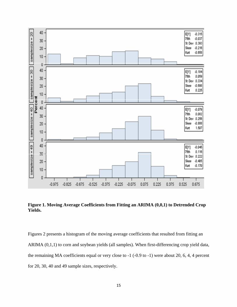
perhaps can be explored by recurring to well‐known theoretical results. Figure 1 presents
a histogram of the moving average coefficients that resulted from fitting an ARIMA (0,0,1)
model to residuals from linearly detrended corn and soybean yields (all samples). After
detrending crop yields it is clear that yields were successfully converted to stationary
processes in about 87, 91, 98 and 100 percent for 20, 30, 40 and 49 samples sizes,
respectively. The counterparts are the MA coefficients close to ‐1 indicating the presence of
a stochastic trend. That these effects are present is cause for thinking that Ng and Perron
(2001) and Perron and Qu (2007) modified tests would be a better method (better size and
power of the tests) to get closer to the time‐series properties of crop yields.
15
Figure 1. Moving Average Coefficients from Fitting an ARIMA (0,0,1) to Detrended Crop Yields.
Figures 2 presents a histogram of the moving average coefficients that resulted from fitting an
ARIMA (0,1,1) to corn and soybean yields (all samples). When first-differencing crop yield data,
the remaining MA coefficients equal or very close to -1 (-0.9 to -1) were about 20, 6, 4, 4 percent
for 20, 30, 40 and 49 sample sizes, respectively.

16
Figure 2. Moving Average Coefficients from Fitting an ARIMA (0,1,1) to Crop Yields (levels).
Modified DF/PP UnitRoot Tests
There are four tests for unit‐roots that were re‐estimated based on the modifications
suggested in Ng and Perron (2001); these tests were “t‐type” tests for unit‐roots and
included the ADF and PP tests of the previous section, and the DFGLS and modified Phillips‐
Perron (MPP). All four tests were estimated using the MAIC selection criterion of Ng and
Perron (2001), so the lag length for the ADF and PP does not necessarily correspond to the
lag‐length used in the previous section. The results are shown in Figures 3‐11. The top
row in each of these figures contains histograms of the values of the t‐statistics for unit‐
root from each of the tests (ADF‐t, PP‐t, DFGLS‐t, and MPP‐t). The t‐test calculated from a
model with a constant is labeled as (C) and from a model with a constant and a trend is
17
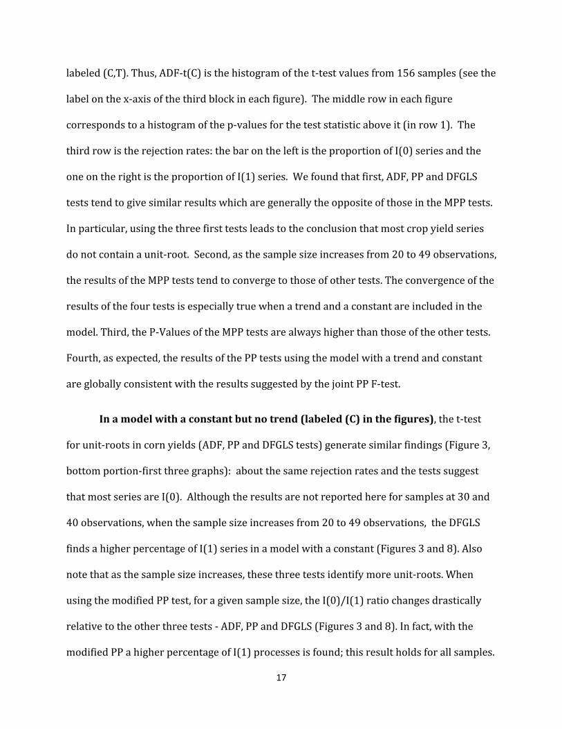
labeled (C,T). Thus, ADF‐t(C) is the histogram of the t‐test values from 156 samples (see the
label on the x‐axis of the third block in each figure). The middle row in each figure
corresponds to a histogram of the p‐values for the test statistic above it (in row 1). The
third row is the rejection rates: the bar on the left is the proportion of I(0) series and the
one on the right is the proportion of I(1) series. We found that first, ADF, PP and DFGLS
tests tend to give similar results which are generally the opposite of those in the MPP tests.
In particular, using the three first tests leads to the conclusion that most crop yield series
do not contain a unit‐root. Second, as the sample size increases from 20 to 49 observations,
the results of the MPP tests tend to converge to those of other tests. The convergence of the
results of the four tests is especially true when a trend and a constant are included in the
model. Third, the P‐Values of the MPP tests are always higher than those of the other tests.
Fourth, as expected, the results of the PP tests using the model with a trend and constant
are globally consistent with the results suggested by the joint PP F‐test.
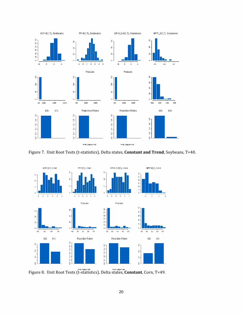
In a model with a constant but no trend (labeled (C) in the figures), the t‐test
for unit‐roots in corn yields (ADF, PP and DFGLS tests) generate similar findings (Figure 3,
bottom portion‐first three graphs): about the same rejection rates and the tests suggest
that most series are I(0). Although the results are not reported here for samples at 30 and
40 observations, when the sample size increases from 20 to 49 observations, the DFGLS
finds a higher percentage of I(1) series in a model with a constant (Figures 3 and 8). Also
note that as the sample size increases, these three tests identify more unit‐roots. When
using the modified PP test, for a given sample size, the I(0)/I(1) ratio changes drastically
relative to the other three tests ‐ ADF, PP and DFGLS (Figures 3 and 8). In fact, with the
modified PP a higher percentage of I(1) processes is found; this result holds for all samples.

18
Figure 3. Unit Root Tests (t‐statistics), Delta states, Constant, Corn, T=20.
Figure 4. Unit Root Tests (t‐stat), Delta states, Corn, Constant and Trend, T=20.

19
Figure 5. Unit Root Tests (t‐statistics), Delta states, Constant, Soybeans, T=20.
Figure 6. Unit Root Tests (t‐statistics), Delta states, Constant and Trend, Soybeans, T=20.
20
Figure 7. Unit Root Tests (t‐statistics), Delta states, Constant and Trend, Soybeans, T=40.
Figure 8. Unit Root Tests (t‐statistics), Delta states, Constant, Corn, T=49.

21
Figure 9. Unit Root Tests (t‐statistics), Delta states, Constant and trend, Corn, T=49.
Figure 10. Unit Root Tests (t‐statistics), Delta states, Constant, Soybeans, T=49.
22
Figure 11. Unit Root Tests (t‐statistics), Delta states, Constant, Corn, T=49.
When using the latter (MPP), as the sample size increases the percentage of I(0) processes
tends to increase (Figures 3 and 8). Note also that the P‐value is generally higher for the
MPP test (Figures 3‐12, middle block). Lastly, we found that the results from the ADF and
PP tests are not consistent with the results obtained with the ADF joint F‐test which found
that about 23% (up to 55% depending on the sample size) of the samples were found to be
trend deterministic or with the Phillips‐Perron F‐test where more than 95% of the series
are trend deterministic at all sample sizes (Table 2).
In a model that includes a constant and a trend (labeled (C,T)) the main highlights for
corn yields are that for a given sample size, most of the series are identified as I(0) when

23
using either ADF, PP or DFGLS tests. These results hold as the sample size increases.
Second, the MPP test gives similar results as in the ADF, PP and DFGLS tests at sample sizes
T= 40 and 49 (Figure 9, results for T=40 not shown). However, at T= 20 & 30, the MPP test
gives opposite results to the ones of ADF, PP and DFGLS tests (i.e. most are I(1) –Figure 4;
results not shown for T=30). As before, the P‐values are higher for the MPP tests (Figure 4
and 9). Note also that the results of the PPs test are consistent with the results of the joint
test in Table 2.
For soybean yields in a model with a constant only (labeled (C)), we found that for
all sample sizes, ADF, PP and DFGLS tests give similar results (i.e., most processes are
identified as I(0) ‐‐Figures 5 and 10). On the contrary, a higher percentage of I(1) yields
has been found when employing the MPP test (Figure 5). However, as the sample size
increases, so does the relative percentage of I(0) yields and almost equals the percentage of
I(1) – Figure 10).
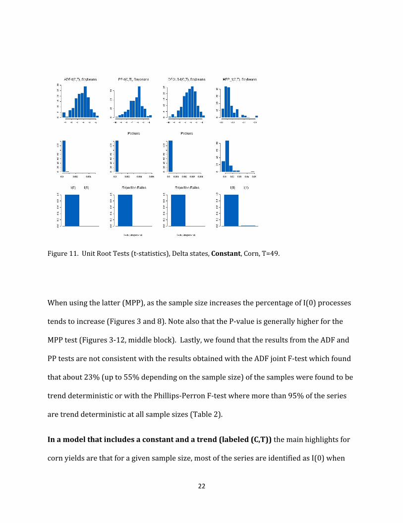
Continuing with soybean yields, in a model with a constant and a trend (labeled
(C,T)), for all samples, ADF, PP and DFGLS tests results are again similar; a majority of I(0)
processes has been found (Figures 6, 7 & 11). On the contrary, employing the MPP test
leads to a higher percentage of I(1) processes (Figure 6). However, as the sample size
increases, from T=20 to T=40, the relative percentage of I(0) increases (Figure 6 & 7). As T
increases to 49 observations, the results of the MPP test become similar to those of the
other tests (i.e., 100% of the processes are found to be I(0) ‐‐Figure 11). Again, the results
obtained when the PP tests are employed are consistent to that of the joint F‐test (Table 2).
24
Discussion
A point that deserves discussion is that at small sample sizes, a large majority of I(1)
processes are found when the MPP tests are employed. As the sample size increases, the
results of the four tests converge (i.e. most processes are I(0)). A question that
instantaneously comes to mind is why the results of the MPP tests are so drastically
different from those of the other tests at small sample sizes? Is it because this particular
test is performing better at small sample sizes or on the contrary, worse? Is this
performance linked to the DGP of the series rather than directly to the sample size? A first
element of response is that our results may support the statement of Ng and Perron (2001)
that “the majority of tests suffer from severe size distortions when the moving‐average
polynomial of the first differenced series has a large negative autoregressive negative root”
(Ng and Perron, 2001, p.1519). In fact, this statement also holds for detrended series. The
general idea is that the performance of unit‐root tests is poor when the error process
presents strongly negative MA terms (Enders, 2010). “The consequence is over‐rejections
of the unit‐root hypothesis” (Ng and Perron, 2001, p.1519). As a matter of fact, we found
that when first‐differencing or detrending crop yield data, the proportion of MA coefficients
close to or equal to ‐1 was higher for small sample sizes (T= 20 and 30) (Figures 1 & 2).
Thus, we conclude that this may indicate that the ADF, PP and DFGLS tests were not
able to identify the presence of unit‐roots in crop yield series at small sample sizes (i.e.
when more filtered series present a MA coefficient close to one). This explains the high
proportion of I(0) found with these tests compared to the results of the MPP tests. This
conclusion deserves an assessment through a Monte Carlo experiment, similar to Ng and

25
Perron (2001) but with smaller sample sizes in a yield‐data coherent framework. Note that
the smallest size that the authors used was 150 observations. Also of interest would be a
closer examination of the performance of the DFGLS‐t statistic in relation to a constant
versus a constant and a trend model specification. The findings here are preliminary but
lead to reasonable results in the first model but not the second.
We believe that the DGP should not be disconnected to what is happening in the
field. Hence, it would be also interesting to link the abundance of series with strongly
negative MA terms to the technological changes or climatic events that occurred in corn
and soybean productions in Southern U.S. Recalling that the counties with small sample
sizes correspond to crop yield observations that start in the early nineties and end today
while for counties with large sample sizes we had observations since the early sixties.
Recalling also that “the presence of the negative MA term means that εt has a one‐unit effect
on yt in period t only” (Enders, 2010, p.220), a MA coefficient that is close to ‐1 may
correspond to a negative shock whose effects are carried to the next crop season. Hence,
we may hypothesize that severe climatic events may have occurred more frequently during
the two last decades.
The search for improved methods to test nonstationarity of yield distributions is
likely to continue. This paper has identified at least one area of future research that may
prove useful in making more definite progress in the identification of yield distributions.
Perhaps future research should also emphasize deeper thinking into the evolving nature of
historical yields and how these can be best related to the theory of nonstochastic processes.
We conducted an exhaustive evaluation testing the paired difference between empirical

26
CDFs generated from an ARIMA(0,1,2) and polynomially detrended yields to address the
question of whether such differences are substantially large to significantly impact risk
estimation. The results found no support for a significant difference between pairs of
empirical CDFs, an issue that deserves closer investigation. Hamilton (1994) suggested to
think in terms of “parsimonious DGPs” and not necessarily about the I(0) or I(1) nature of
the data. Perhaps future studies of nonstationary yields will shed more light on this
thinking.

27
References
Atwood, J., S. Shaik, and M. Watts. “Are Crop Yields Normally Distributed? A Reexamination.” American Journal of Agricultural Economics, 85,4(November 2003):888‐901.
Bessler, D. "Aggregated Personalistic Beliefs on Yields of Selected Crops Estimated Using ARIMA Processes." American Journal of Agricultural Economics. 62(November 1980):666‐74.
Day, R.H. “Probability Distributions of Field Crop Yields.” Journal of Farm Economics, 47,3(August 1965):713‐741.
Dufour, J.M., and M. King. “Optimal Invariant Tests for Autocorrelation Coefficient in Linear Regressions with Stationary and Nonstationary Errors,” Journal of Econometrics, 47(1991):115‐143.
DeJong, D.N., J.C. Nankervis, N.E. Savin, and C.H. Whiteman. “The Power Problem of Unit Root Tests in Time Series with Autoregressive Errors,” Journal of Econometrics, 53(1992):323‐343.
Dickey, D.A. and W.A. Fuller. “Distribution of the Estimators for Autoregressive Time Series with a Unit Root.” Journal of the American Statistical Association, (1979): 427–431.
Elliot, G., T.J. Rothenberg, and J.H. Stock. “Efficient Tests for an Autoregressive Unit Root,” Econometrica, 64(1996):813‐836.
Enders, W. Applied Econometric Time Series. Wiley Series in Probability and Mathematical Statistics. New York: John Wiley & Sons, 1995 and 2010.
Foote, R. J., and L. H. Bean. “Are Yearly Variations in Crop Yields Really Random?” Journal of Agricultural Economic Resources, 3(1951):23‐30
Gallagher, P. “U.S. Corn Yield Capacity and Probability: Estimation and Forecasting with Nonsymmetric Disturbances.” North Central Journal of Agricultural Economics, 8,1(January 1986:)109‐22.
____. “U.S. Soybean yields: Estimation and Forecasting with Nonsymmetric Disturbances.” American Journal of Agricultural Economics, 69,4(November 1987):796‐803.
Goodwin, B. K., and A.P. Ker. “Nonparametric Estimation of Crop Yield Distributions: Implications for Rating Group‐Risk Crop Insurance Contracts.” American Journal of Agricultural Economics, 80,1(February 1998):139‐53.
Haldrup, N. and M. Jansson. “Improving Size and Power in Unit Root Testing.” In T.C. Mills, K. Patterson (eds.), Econometric Theory, Vol. 1 of Palgrave Handbook of Econometrics, Ch. 7, (2006) pp. 252‐277. Palgrave MacMillan, Basingstoke.
Hamilton, J.D. Time Series Analysis. Princeton, NJ: Princeton University Press, 1994.

28
Harri, A. Erdem, C., K. H. Coble, and T. O. Knight. “Crop Yield Distributions: A Reconciliation of Previous Research and Statistical Tests for Normality.” Review of Agricultural Economics, No. 1 (2008): 163‐182.
Kaylen, M.S., and S.S. Koroma. “Trend, Weather Variables, and the Distribution of U.S. Corn Yields.” Review of Agricultural Economics, 13,2(July 1991):249‐58.
Ker, A.P., and B. K. Goodwin. “Nonparametric Estimation of Crop Insurance Rates Revisited.” American Journal of Agricultural Economics, 83(May 2000):463‐478.
Lopez, J.H. “The Power of the ADF test,” Economics Letters, 57(1997):5‐10.
Lupi, C. “Unit Root CADF Testing in R.” Journal of Statistical Software, 32, 2 (2009): 1‐19. URL http://www.jstatsoft.org/v32/i02/.
Maradiaga, D.I. (2010). Stochastic Trends in Crop Yield Density Estimation. Master's Thesis, Louisiana State University, Baton Rouge, LA. 67p.
Moss, C.B., and J.S. Shonkwiler. “Estimating Yield Distributions with a Stochastic Trend and Nonnormal Errors.” American Journal of Agricultural Economics, 75,4(November 1993):1056‐62.
National Agricultural Statistics Service (NASS‐USDA). Historical Corn and Soybean Yields at the County Level from Arkansas, Louisiana, Mississippi, Missouri and Texas. Downloaded on January 10 2011 from: nass.usda.gov/Data_and_Statistics/Quick_Stats/
Nelson, C.H. “The Influence of Distributional Assumptions on the Calculation of Crop Insurance Premia.” North Central Journal of Agricultural Economics, 12(January 1990):71‐78.
Nelson, C.H., and P.V. Preckel. “The Conditional Beta Distribution as a Stochastic Production Function.” American Journal of Agricultural Economics, 71,2(May 1989):370‐78.
Ng, S., and P. Perron (1995): “Unit Root Tests in ARMA Models with Data Dependent Methods for the Selection of the Truncation Lag,” Journal of the American Statistical Association, 90, 268–281.
_____“Lag Length Seleccion and the Construction of Unit Root Tests with Good Size and Power,” Econometrica, Vol. 69, No. 6 (November, 2001), 1519–1554.
Norwood, B., M.C. Roberts, and J.L. Lusk “Ranking Crop Yield Models Using out‐of‐Sample Likelihood Functions.” American Journal of Agricultural Economics, 86,4(2004):1032‐43.
Perron, P., and S. Ng (1996): “Useful Modifications to Unit Root Tests with Dependent Errors and their Local Asymptotic Properties,” Review of Economic Studies, 63, 435–465.
Perron, P. and Z. Qu. “A simple modification to improve the finite sample properties of Ng and Perron’s unit root tests. Economic Letters, 94 (2007): 12‐19.
Phillips, P.C., "Time Series Regression with Unit Roots," Econometrica, 55,2(1987), 277‐302.
29
Phillips P.C. and P. Perron. “Testing for a Unit Root in Time Series Regression.” Biometrika, 75,2(June, 1988):335‐346.
Ramírez, O. A. “Estimation and Use of a Multivariate Parametric Model for Simulating Heteroskedastic, Correlated, Nonnormal Random Variables: The Case of Corn Belt Corn, Soybeans, and Wheat Yields.” American Journal of Agricultural Economics, 79,1(February 1997):191‐205.
Said and Dickey, 1984. S.E. Said and D.A. Dickey , Testing for unit roots in autoregressive moving average models of unknown order. Biometrika, 71 (1984), pp. 599–607.
Sherrick, B.J., F.C. Zanini, G.D. Schnitkey, and S.H. Irwin. “Crop Insurance Valuation under Alternative Yield Distributions.” American Journal of Agricultural Economics, 86,2(May 2004):406‐19.
Schwert, G. W. (1989): “Tests for Unit Roots: A Monte Carlo Investigation,” Journal of Business and Economic Statistics, 7, 147–160.
Stock, J.H. “A Class of Tests for Integration and Cointegration,” Manuscript, Harvard University, 1990.
Turvey, C.G., and J. Zhao. “Parametric and Non‐Parametric Crop Yield Distributions and Their Effects on All‐Risk Crop Insurance Premiums.” Working Paper WP 99/05, Department of Food, Agricultural and Resource Economics, University of Guelph, Guelph, January 1999.
Zapata, H.O., and A.N. Rambaldi. “Effects of Data Transformation on Stochastic Properties of Economic Data,” Paper presented at the annual meetings of the American Agricultural Economics Association, Baton Rouge, Louisiana, July 1989.
Top Related