


Languages
Pages
Legal

Query OptimizationIntroduction to DatabasesCompSci 316 Spring 2017

Announcements (Mon., Mar. 27)
• Homework #3 • 3.3, 3.4, and 3.5 due Wednesday, March 29
• Project• Milestone 2 due today
• Submit both on sakai
2
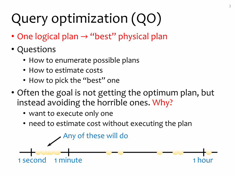
Query optimization (QO)• One logical plan → “best” physical plan• Questions• How to enumerate possible plans• How to estimate costs• How to pick the “best” one
• Often the goal is not getting the optimum plan, but instead avoiding the horrible ones. Why?• want to execute only one• need to estimate cost without executing the plan
3
1 second 1 hour1 minute
Any of these will do
Steps for cost based QO4
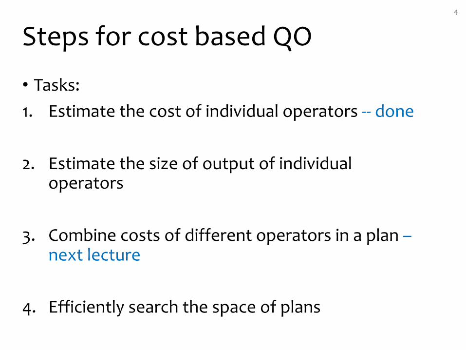
• Tasks:1. Estimate the cost of individual operators -- done
2. Estimate the size of output of individual operators
3. Combine costs of different operators in a plan –next lecture
4. Efficiently search the space of plans
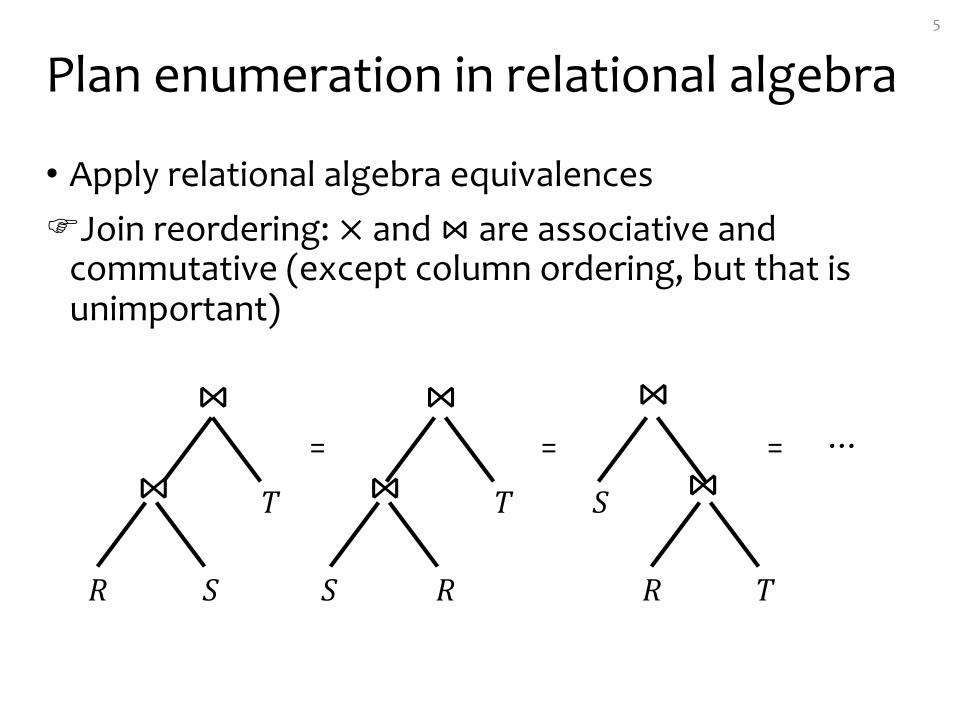
Plan enumeration in relational algebra
• Apply relational algebra equivalencesFJoin reordering: × and ⋈ are associative and
commutative (except column ordering, but that is unimportant)
5
⋈
⋈
𝑅 𝑆
𝑇
⋈
⋈
𝑆 𝑅
𝑇
⋈
⋈
𝑅 𝑇
𝑆
…= = =
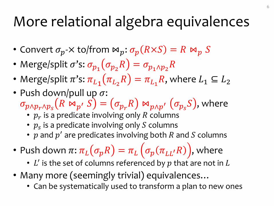
More relational algebra equivalences
• Convert 𝜎(-× to/from ⋈(: 𝜎( 𝑅×𝑆 = 𝑅 ⋈( 𝑆• Merge/split 𝜎’s: 𝜎(* 𝜎(+𝑅 = 𝜎(*∧(+𝑅• Merge/split 𝜋’s: 𝜋./ 𝜋.+𝑅 = 𝜋.*𝑅, where 𝐿/ ⊆ 𝐿2• Push down/pull up 𝜎:𝜎(∧(3∧(4 𝑅 ⋈(5 𝑆 = 𝜎(3𝑅 ⋈(∧(5 𝜎(4𝑆 , where• 𝑝7 is a predicate involving only 𝑅 columns• 𝑝8 is a predicate involving only 𝑆 columns• 𝑝 and 𝑝9 are predicates involving both 𝑅 and 𝑆 columns
• Push down 𝜋: 𝜋. 𝜎(𝑅 = 𝜋. 𝜎( 𝜋..5𝑅 , where• 𝐿9 is the set of columns referenced by 𝑝 that are not in 𝐿
• Many more (seemingly trivial) equivalences…• Can be systematically used to transform a plan to new ones
6
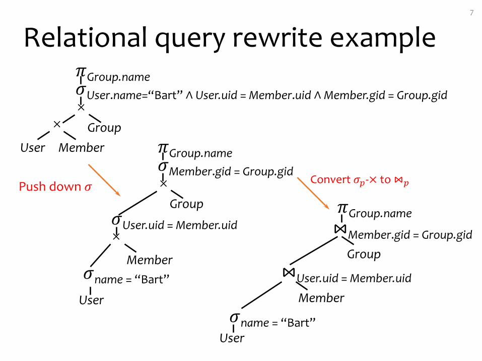
Relational query rewrite example7
𝜋Group.name𝜎User.name=“Bart” ∧ User.uid = Member.uid ∧Member.gid = Group.gid×
MemberGroup×
User 𝜋Group.name𝜎Member.gid = Group.gid×
Member
Group
×
User
𝜎User.uid = Member.uid
𝜎name = “Bart”
Push down 𝜎𝜋Group.name⋈Member.gid = Group.gid
Member
Group
User
⋈User.uid = Member.uid
𝜎name = “Bart”
Convert 𝜎(-× to ⋈(
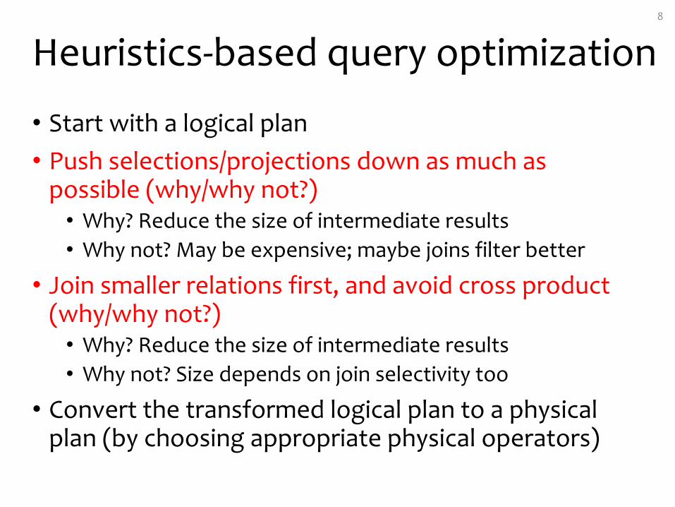
Heuristics-based query optimization
• Start with a logical plan• Push selections/projections down as much as
possible (why/why not?)• Why? Reduce the size of intermediate results• Why not? May be expensive; maybe joins filter better
• Join smaller relations first, and avoid cross product (why/why not?)• Why? Reduce the size of intermediate results• Why not? Size depends on join selectivity too
• Convert the transformed logical plan to a physical plan (by choosing appropriate physical operators)
8
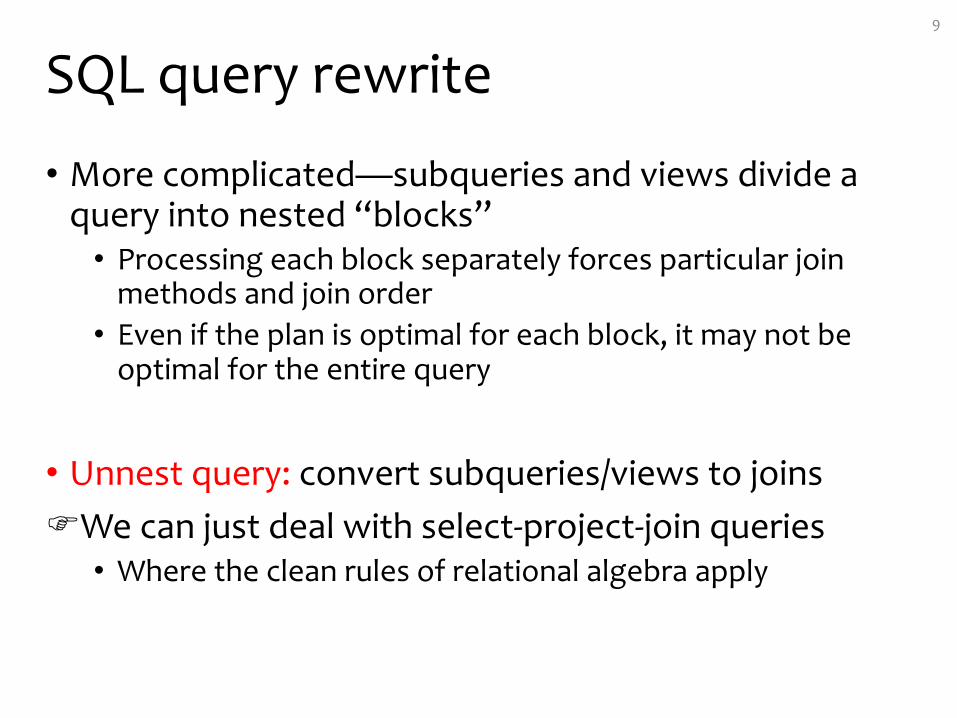
SQL query rewrite
• More complicated—subqueries and views divide a query into nested “blocks”• Processing each block separately forces particular join
methods and join order• Even if the plan is optimal for each block, it may not be
optimal for the entire query
• Unnest query: convert subqueries/views to joinsFWe can just deal with select-project-join queries• Where the clean rules of relational algebra apply
9
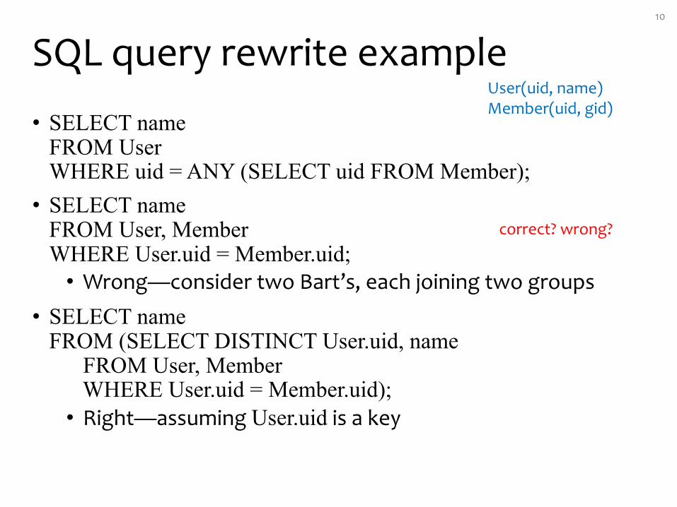
SQL query rewrite example
• SELECT nameFROM UserWHERE uid = ANY (SELECT uid FROM Member);• SELECT name
FROM User, MemberWHERE User.uid = Member.uid;• Wrong—consider two Bart’s, each joining two groups
• SELECT nameFROM (SELECT DISTINCT User.uid, name
FROM User, MemberWHERE User.uid = Member.uid);• Right—assuming User.uid is a key
10
correct? wrong?
User(uid, name)Member(uid, gid)
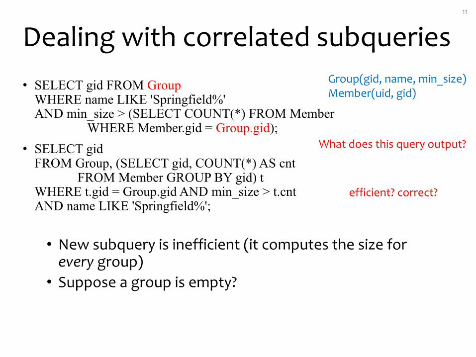
Dealing with correlated subqueries• SELECT gid FROM Group
WHERE name LIKE 'Springfield%'AND min_size > (SELECT COUNT(*) FROM Member
WHERE Member.gid = Group.gid);• SELECT gid
FROM Group, (SELECT gid, COUNT(*) AS cntFROM Member GROUP BY gid) t
WHERE t.gid = Group.gid AND min_size > t.cntAND name LIKE 'Springfield%';
• New subquery is inefficient (it computes the size for every group)• Suppose a group is empty?
11
Group(gid, name, min_size)Member(uid, gid)
efficient? correct?
What does this query output?
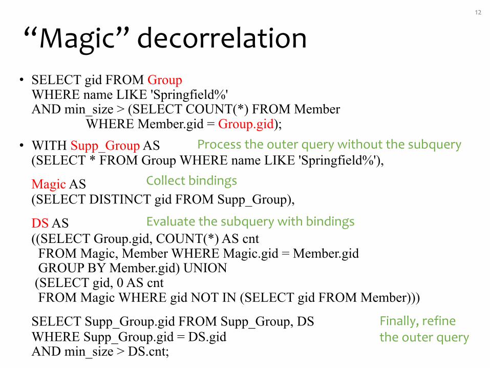
“Magic” decorrelation• SELECT gid FROM Group
WHERE name LIKE 'Springfield%'AND min_size > (SELECT COUNT(*) FROM Member
WHERE Member.gid = Group.gid);• WITH Supp_Group AS
(SELECT * FROM Group WHERE name LIKE 'Springfield%'),
Magic AS(SELECT DISTINCT gid FROM Supp_Group),
DS AS((SELECT Group.gid, COUNT(*) AS cntFROM Magic, Member WHERE Magic.gid = Member.gidGROUP BY Member.gid) UNION
(SELECT gid, 0 AS cntFROM Magic WHERE gid NOT IN (SELECT gid FROM Member)))
SELECT Supp_Group.gid FROM Supp_Group, DSWHERE Supp_Group.gid = DS.gidAND min_size > DS.cnt;
12
Process the outer query without the subquery
Collect bindings
Evaluate the subquery with bindings
Finally, refinethe outer query
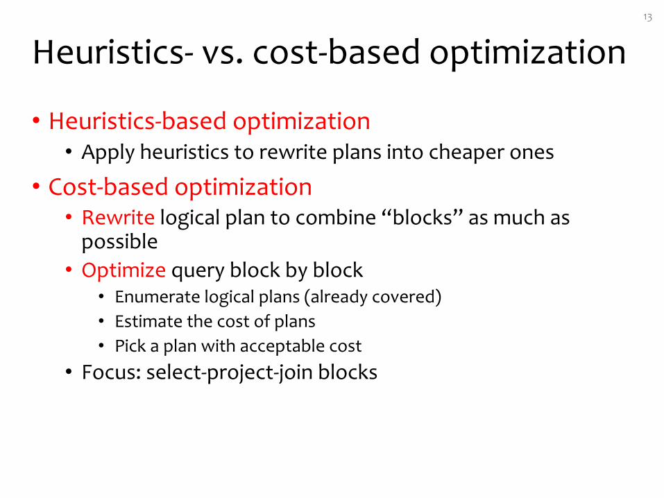
Heuristics- vs. cost-based optimization
• Heuristics-based optimization• Apply heuristics to rewrite plans into cheaper ones
• Cost-based optimization• Rewrite logical plan to combine “blocks” as much as
possible• Optimize query block by block
• Enumerate logical plans (already covered)• Estimate the cost of plans• Pick a plan with acceptable cost
• Focus: select-project-join blocks
13
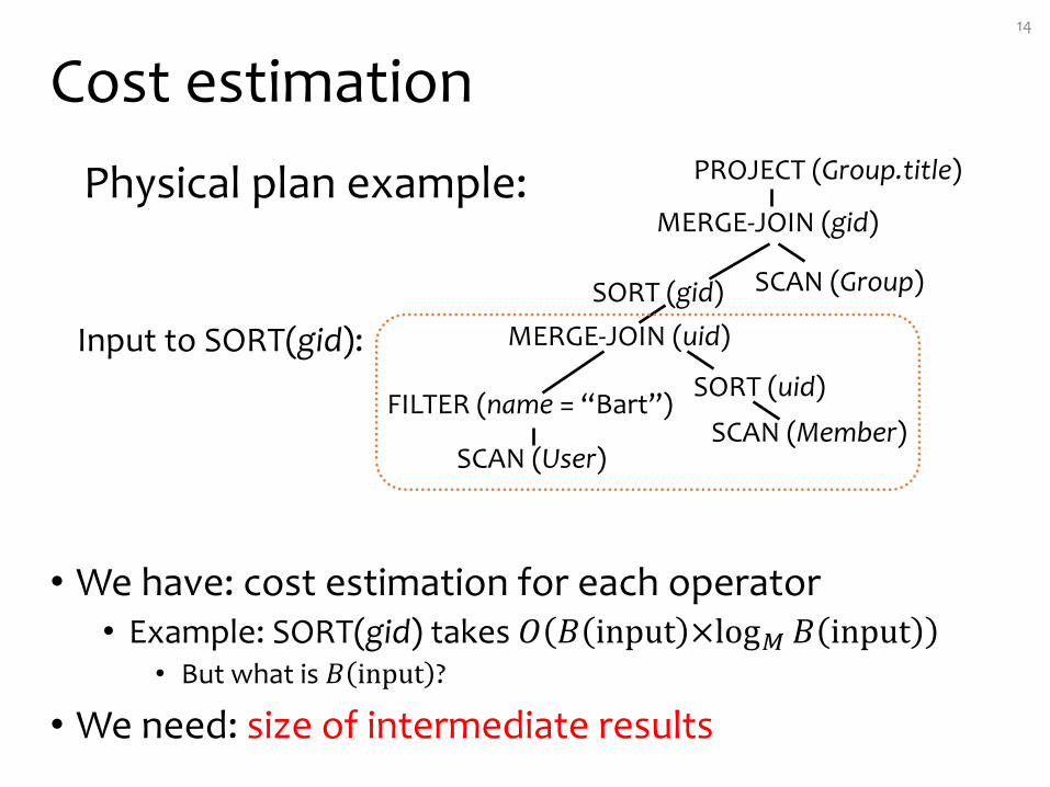
Cost estimation
• We have: cost estimation for each operator• Example: SORT(gid) takes 𝑂 𝐵 input ×logD 𝐵 input
• But what is 𝐵 input ?
• We need: size of intermediate results
14
PROJECT (Group.title)
MERGE-JOIN (gid)
SCAN (Group)SORT (gid)MERGE-JOIN (uid)
SCAN (Member)
SORT (uid)
SCAN (User)
FILTER (name = “Bart”)
Physical plan example:
Input to SORT(gid):
15
http://www.learningresources.com/product/estimation+station.do
Cardinality estimation
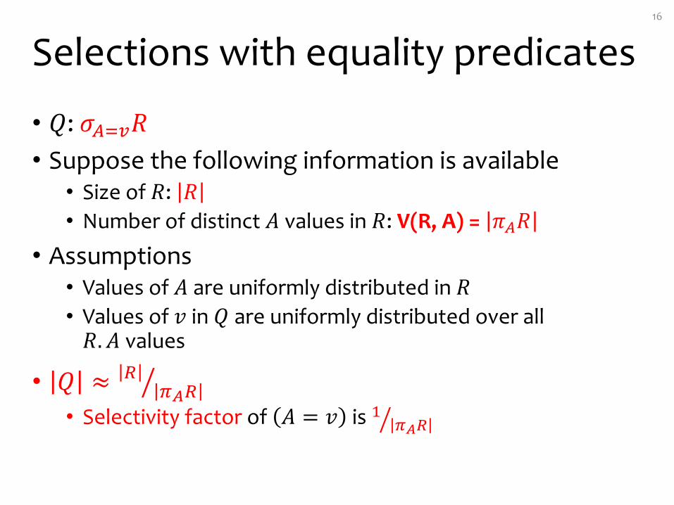
Selections with equality predicates
• 𝑄: 𝜎FGH𝑅• Suppose the following information is available• Size of 𝑅: 𝑅• Number of distinct 𝐴 values in 𝑅: V(R, A) = 𝜋F𝑅
• Assumptions• Values of 𝐴 are uniformly distributed in 𝑅• Values of 𝑣 in 𝑄 are uniformly distributed over all 𝑅. 𝐴values
• 𝑄 ≈ NOPNQ
• Selectivity factor of 𝐴 = 𝑣 is / OPNQ
16
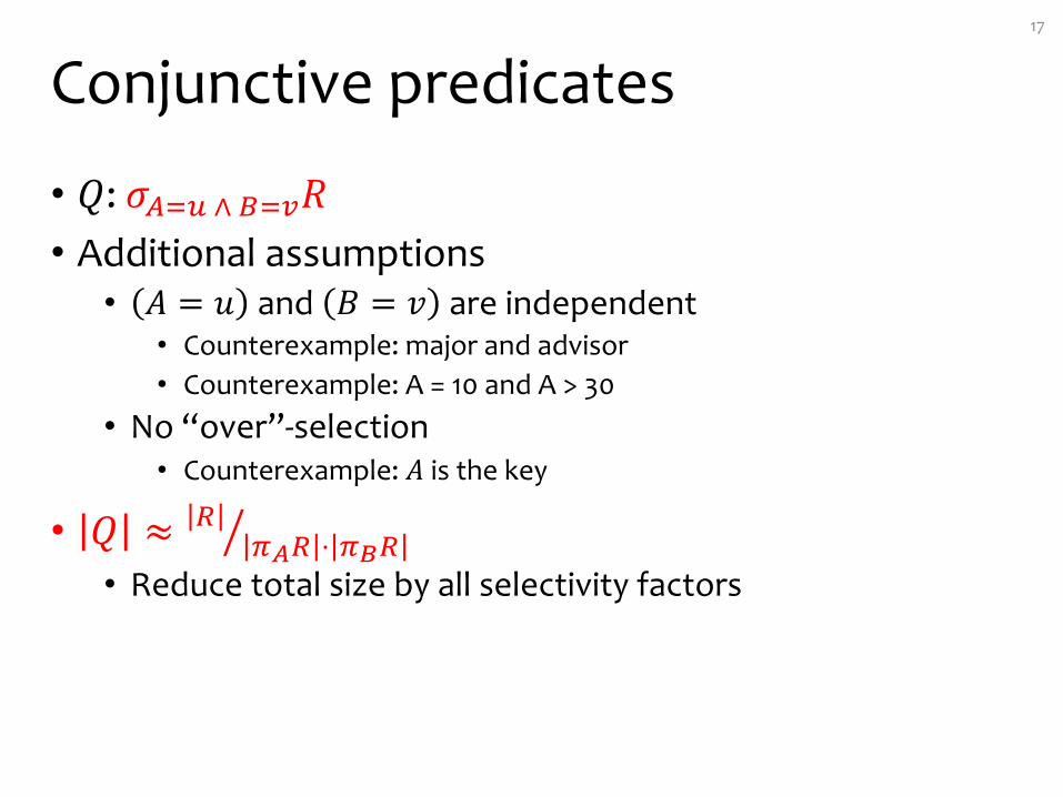
Conjunctive predicates
• 𝑄: 𝜎FGR∧SGH𝑅• Additional assumptions• 𝐴 = 𝑢 and 𝐵 = 𝑣 are independent
• Counterexample: major and advisor• Counterexample: A = 10 and A > 30
• No “over”-selection• Counterexample: 𝐴 is the key
• 𝑄 ≈ NOPN ⋅ OVNQ
• Reduce total size by all selectivity factors
17
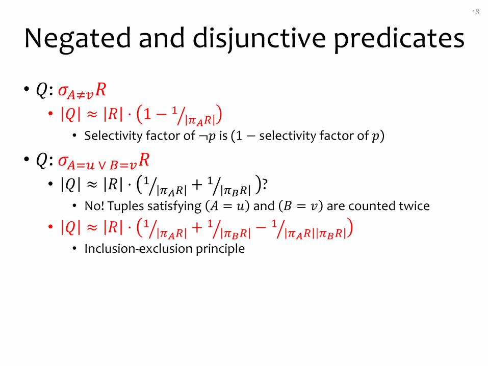
Negated and disjunctive predicates
• 𝑄: 𝜎FWH𝑅• 𝑄 ≈ 𝑅 ⋅ 1 − /
OPNQ• Selectivity factor of ¬𝑝 is (1 − selectivity factor of 𝑝)
• 𝑄: 𝜎FGR∨SGH𝑅• 𝑄 ≈ 𝑅 ⋅ /
OPNQ + /OVNQ ?
• No! Tuples satisfying 𝐴 = 𝑢 and 𝐵 = 𝑣 are counted twice
• 𝑄 ≈ 𝑅 ⋅ /OPNQ + /
OVNQ − /OPN OVNQ
• Inclusion-exclusion principle
18
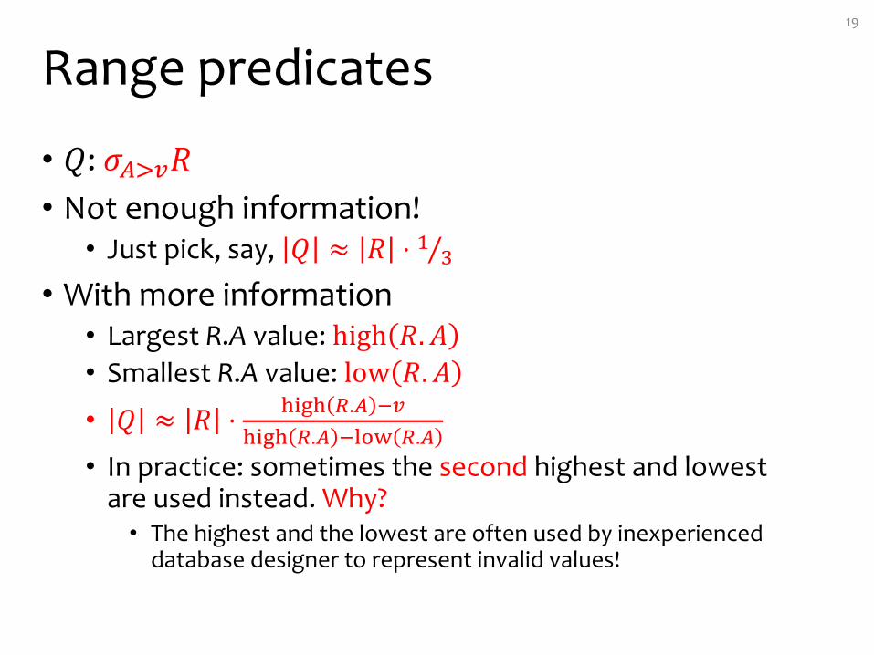
Range predicates
• 𝑄: 𝜎F]H𝑅• Not enough information!• Just pick, say, 𝑄 ≈ 𝑅 ⋅ / ^⁄
• With more information• Largest R.A value: high 𝑅. 𝐴• Smallest R.A value: low 𝑅. 𝐴• 𝑄 ≈ 𝑅 ⋅ bcdb N.F eH
bcdb N.F efgh N.F• In practice: sometimes the second highest and lowest
are used instead. Why?• The highest and the lowest are often used by inexperienced
database designer to represent invalid values!
19
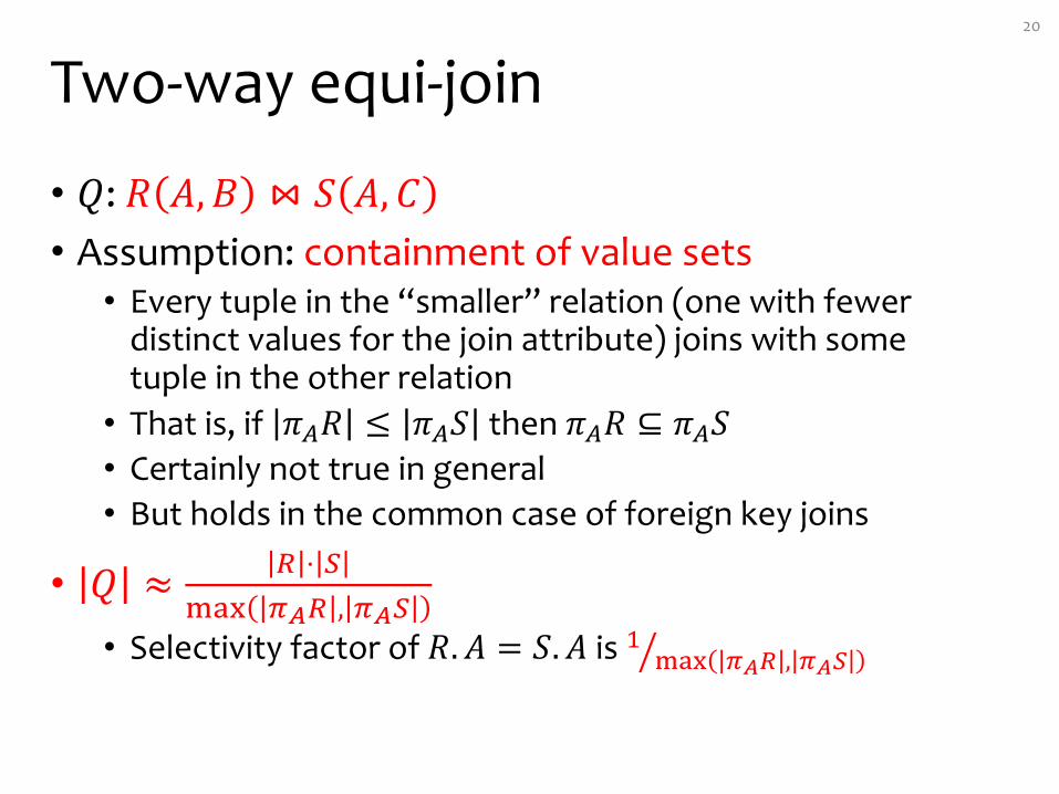
Two-way equi-join
• 𝑄: 𝑅 𝐴, 𝐵 ⋈ 𝑆 𝐴, 𝐶• Assumption: containment of value sets• Every tuple in the “smaller” relation (one with fewer
distinct values for the join attribute) joins with some tuple in the other relation• That is, if 𝜋F𝑅 ≤ 𝜋F𝑆 then 𝜋F𝑅 ⊆ 𝜋F𝑆• Certainly not true in general• But holds in the common case of foreign key joins
• 𝑄 ≈ N ⋅ lmno OPN , OPl
• Selectivity factor of 𝑅. 𝐴 = 𝑆. 𝐴 is / mno OPN , OPlQ
20
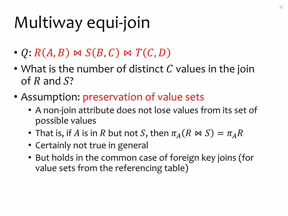
Multiway equi-join
• 𝑄: 𝑅 𝐴, 𝐵 ⋈ 𝑆 𝐵, 𝐶 ⋈ 𝑇 𝐶, 𝐷• What is the number of distinct 𝐶 values in the join
of 𝑅 and 𝑆?• Assumption: preservation of value sets• A non-join attribute does not lose values from its set of
possible values• That is, if 𝐴 is in 𝑅 but not 𝑆, then 𝜋F 𝑅 ⋈ 𝑆 = 𝜋F𝑅• Certainly not true in general• But holds in the common case of foreign key joins (for
value sets from the referencing table)
21
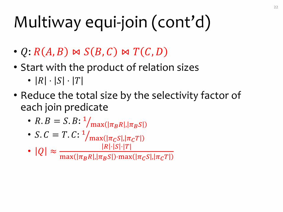
Multiway equi-join (cont’d)
• 𝑄: 𝑅 𝐴, 𝐵 ⋈ 𝑆 𝐵, 𝐶 ⋈ 𝑇 𝐶, 𝐷• Start with the product of relation sizes • 𝑅 ⋅ 𝑆 ⋅ 𝑇
• Reduce the total size by the selectivity factor of each join predicate• 𝑅. 𝐵 = 𝑆. 𝐵: / mno OVN , OVlQ• 𝑆. 𝐶 = 𝑇. 𝐶: / mno Oql , OqrQ• 𝑄 ≈ N ⋅ l ⋅|r|
mno OVN , OVl ⋅mno Oql , Oqr
22

Cost estimation: summary
• Using similar ideas, we can estimate the size of projection, duplicate elimination, union, difference, aggregation (with grouping)• Lots of assumptions and very rough estimation• Accurate estimate is not needed• Maybe okay if we overestimate or underestimate
consistently• May lead to very nasty optimizer “hints”
SELECT * FROM User WHERE pop > 0.9;SELECT * FROM User WHERE pop > 0.9 AND pop > 0.9;
• Not covered: better estimation using histograms
23
Search strategy24
http://1.bp.blogspot.com/-Motdu8reRKs/TgyAi4ki5QI/AAAAAAAAAKE/mi8ejfZ8S7U/s1600/cornMaze.jpg
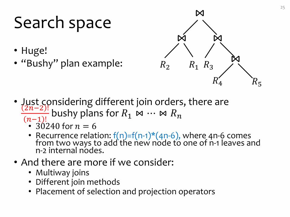
Search space• Huge!• “Bushy” plan example:
• Just considering different join orders, there are 2te2 !te/ !
bushy plans for 𝑅/ ⋈ ⋯ ⋈ 𝑅t• 30240 for 𝑛 = 6• Recurrence relation: f(n)=f(n-1)*(4n-6), where 4n-6 comes
from two ways to add the new node to one of n-1 leaves and n-2 internal nodes.
• And there are more if we consider:• Multiway joins• Different join methods• Placement of selection and projection operators
25⋈
𝑅2 𝑅/ 𝑅^𝑅} 𝑅~
⋈ ⋈⋈
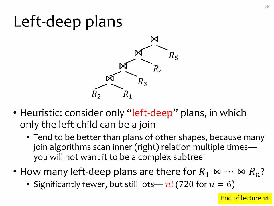
Left-deep plans
• Heuristic: consider only “left-deep” plans, in which only the left child can be a join• Tend to be better than plans of other shapes, because many
join algorithms scan inner (right) relation multiple times—you will not want it to be a complex subtree
• How many left-deep plans are there for 𝑅/ ⋈ ⋯ ⋈ 𝑅t?• Significantly fewer, but still lots— 𝑛! (720 for 𝑛 = 6)
26
⋈
𝑅2 𝑅/𝑅^
𝑅}𝑅~⋈
⋈⋈
End of lecture 18
Top Related