


Languages
Pages
Legal


1
Quasi-stationarity of centennial Northern Hemisphere midlatitude winter storm tracks
Lan Xia, Hans von Storch, Frauke Feser Institute of Coastal Research, Helmholtz-Zentrum Geesthacht, Geesthacht, Germany Abstract: The winter storm activity on the Northern Hemisphere during the last one thousand years in a global
climate simulation was analyzed by determining all midlatitude storms and their tracks, then consecutively
clustering them for hundred years’ segments. Storm track clusters with longest lifetime and largest deepening
rates are found over the oceans. The numbers of extratropical winter storms exhibit notable yearly variability but
hardly any variability on centennial time scales. The clusters of these storm tracks also show only small
differences between the centuries. The numbers of members in neighboring oceanic clusters are negatively
correlated. A linear relationship was found between the numbers of members per storm track clusters over the
Pacific or Atlantic Ocean and seasonal mean atmospheric circulation patterns by a canonical correlation analysis
(CCA).
1. Introduction
There is great interest in the issue of changing statistics of extratropical cyclones because of the impacts
associated with the passage of such storms, in particular related to strong wind and heavy precipitation.
Therefore many studies deal with perspectives of changing storm statistics in the course of emerging
anthropogenic climate change (e.g., Schubert et al. 1998; Ulbrich and Christoph 1999; Pinto et al. 2007).
However, for assessing the significance of expected future changes, knowledge about the natural variability of
storminess is needed (IDAG 2005). But most analysis of recent and ongoing change of extratropical storm
activity concentrated on recent decades re-analyses such as Sickmöller et al. (2000) and Weisse et al. (2005), or
on the last century such as Alexandersson et al. (1998) and Matulla et al. (2008) who made use of proxies based
on air pressure statistic. Only Fischer-Bruns et al. (2005) examined multi-centennial data – from coupled
atmosphere-ocean global climate model (GCM) simulations subject to estimated external (volcanic, solar and
anthropogenic) forcing. They showed that the storm frequency had no noteworthy long-term trends until
recently. In particular no obvious link between temperature variations and extratropical storm activity emerged.
We examine in this paper a similar GCM simulation, this time extending for almost 1000 years, and we study the
statistics through the lens of regional clustering and frequency of storm tracks. It has been shown previously that
the temperature variations simulated by the model (von Storch et al. 2004) is relatively strong, albeit within the

2
range of what is considered plausible for the past millennium (Moberg et al. 2005), so that we may expect the
model to simulate also the century-to-century variability of other quantities, such as mid-latitude storminess.
This study is based on the availability of millennial simulations, which by now are routinely computed after their
first appearance in the late 1990s (von Storch et al. 1997). This long simulation mostly operates with spatial
resolutions which are suitable for extratropical storms, but not for tropical cyclones. Since it has been used and
examined by various researchers on midlatitude storms (Fischer-Bruns et al. 2005), we limit ourselves to such
midlatitude baroclinic storms.
Unfortunately, the spatial resolution of this simulation is relatively coarse, namely T30, and the output is stored
only every 12 hours. Jung et al. (2006) state that extratropical cyclone numbers within low horizontal resolution
model data are 40% smaller compared with reanalysis data. Uncertainties of cyclone frequency also rise due to
the coarse temporal resolution (Zolina and Gulev 2002). However, previous analyses have employed just this
configuration, such as Raible and Blender (2004) and Fischer Bruns et al. (2005). When assessing storm activity
in terms of variance of 500 hPa height, Stendel and Roeckner (1998) found that T30 generates reasonable
patterns and the deviations are less than 10% compared to ERA/ECMWF reanalysis data. A comparison of our
results with other tracking studies is difficult as different tracking methods use different settings. Important is,
however, that the spatial patterns and the relative frequencies of the different tracks are comparable. The
intention of this study is to determine and discuss the variability of storm tracks from century to century. We
argue that the underestimation of the total number and length of tracks acts in the same way throughout the
simulation: our track numbers may be biased negatively, but uniformly, so that the variability should hardly be
affected.
Various automatic tracking algorithms for describing cyclone activity in long-term datasets are available (Murray
and Simmonds, 1991; Hodges, 1994, 1995; Serreze, 1995; Blender et al., 1997; Muskulus and Jacob, 2005;
Wernli and Schwierz, 2006; Rudeva and Gulev, 2007; Zahn and von Storch, 2008a). We adopt in our study
Hodges (1994, 1995 and 1999) well-documented and frequently applied method. The cluster analysis was
developed for sorting objects into different categories, and can of course be applied to cyclones, e.g. Blender et
al. (1997) and Sickmöller et al. (2000) for North Atlantic baroclinic storms, Elsner (2003), Nakamura et al.
(2009) and Chu et al. (2010) for tropical storms.

3
How storm track activity relates to changes of circulation has been studied often: the effect of the North Atlantic
Oscillation (NAO) (Hurrell 1995, Ulbrich and Christoph 1999, Gulev et al. 2001, Pinto et al. 2007 and Raible et
al. 2007) on storm statistics has been studied; also the effects of the Southern Oscillation (SO) (Sickmöller et al.
2000), the North Pacific Oscillation (PNA) (Christoph and Ulbrich 2000, Sickmöller et al. 2000, and Gulev et al.
2001) as well as anomalies of midlatitude sea surface temperature (SST) anomalies (Brayshaw et al. 2008). In
this paper, variability of Northern Hemisphere extratropical storms and its relation to changes in winter
circulation is studied. This is done with the help of a Canonical Correlation Analysis of seasonal anomalies of
mean sea level pressure fields (MSLP) and the time-variable number of members in the storm track clusters.
The long-term simulation dataset, obtained with the coupled atmosphere-ocean GCM ECHO-G exposed to time
variable solar, volcanic and greenhouse-gas forcing of the last millennium, is described in section 2. In section
3.1 tracking results using the Lagrangian-type tracking algorithm of Hodges (1994, 1995, and 1999) are shown
and compared with results derived from NCEP/NCAR reanalysis data in order to evaluate the model simulation.
Time series of cyclone numbers for the 990 years (quasi-millennium) and for the 10 centuries are also shown. In
section 3.2 tracks are clustered into ten groups by the K-means clustering method; characteristics such as life
span, frequency, or intensity are analyzed for each cluster. Century-to-century variability of cyclones for each
cluster is also analyzed. Interactions of storm counts between different clusters are studied in section 3.3.
Variations of the numbers of members of the clusters in the marine sectors of the North Pacific and North
Atlantic are related to mean winter circulation anomalies in section 3.4. In section 4 results are discussed and
conclusions are drawn.
2. Data and Methods
2.1 Data
The quasi-millennial (years 1000-1990) simulation which data is used in this study has been run with the global
climate model ECHO-G (Min et al., 2005 a, b) that combines the atmospheric model ECHAM4 (Roeckner et al.
1996) and ocean model HOPE-G (Wolff et al. 1997). For the atmospheric part the horizontal resolution is T30
(about 3.75°) and for the ocean T42 (about 2.8°). There are 19 (20) levels for the atmosphere (ocean). The output
is stored every 12 hours. The estimated historical forcing for driving the model such as solar variations, CO2 and
CH4 concentrations as well as volcanic effects have been described previously by von Storch et al. (2004) and
Zorita et al. (2005). ECHO-G simulations have been found skillfully in simulating the seasonal mean
climatology and inter-annual variability of mean sea level pressure and surface temperature (Min et al. 2005 a, b;

4
Gouirand et al. 2007). The atmospheric circulation of the Northern Hemisphere in winter including the NAO
pattern is simulated realistically by ECHO-G (Min et al., 2005b). The North Atlantic sea level pressure
anomalies and response to the El Nino Southern Oscillation (ENSO) are similar to observed patterns and other
climate reconstructions (Gouirand et al. 2007).
Examinations of shorter simulations done with ECHO-G have shown that the grid resolution of T30 is sufficient
to study midlatitude baroclinic cyclones (Stendel and Roeckner 1998, Raible and Blender 2004, Fischer-Bruns et
al. 2005). The storm tracks were found to agree well with ERA-15/ECMWF reanalysis data (Stendel and
Roeckner, 1998).
The key added value of this simulation is the homogeneous presentation of a possible development during the
last millennium; obviously a validation of the simulation is hardly possible. However, with respect to the
development of Northern Hemisphere temperature, comparisons with different proxy reconstructions are
possible, ranging from tree ring data to borehole temperatures (González-Rouco et al. 2003, Tan et al. 2009).
These indicate that this simulations is within the envelope of suggestions of past temperature development. Other
simulations extending over 1000 and more years also exhibit qualitatively similar developments. Some have
argued that ECHO-G temperature variations would be too strong, however, which would not question our main
conclusion namely that the mid-latitude winter storm activity is remarkably stationary on time scales of 100
years (see below).
2.2 Cyclone tracking
For cyclone identification and tracking, the automatic tracking algorithm developed by Hodges (1994, 1995, and
1999) is applied. This algorithm has widely been used to study climatology of extratropical cyclones (Hoskins
and Hodges 2002, 2005), tropical storms and monsoon depressions (Hodges 1999), or specific cyclones such
polar lows (Xia et al. 2012). In this study, only winter cyclones (DJF) at mid-latitudes (≥30° N) on the Northern
Hemisphere (NH) are considered.
The tracking is done with mean sea level pressure (MSLP) fields of ECHO-G simulation. Before tracking,
wavenumbers less than or equal to 5 are subtracted for removing large-scale features (Hoskins and Hodges
2002). Then the tracking algorithm determines all minima below -1 hPa in the filtered MSLP fields. Minima are
5
connected to form tracks if their distance is less than 12° (about 1333 km) within 12 hours. Minimum lifetimes
of tracks are set to 2 days.
For the temporal resolution, no ad-hoc process is used to interpolate the 12-hourly MSLP fields into shorter time
steps (as e.g. Murray and Simmonds 1991, Zolina and Gulev 2002 have done). For getting smooth tracks, B-
spline interpolation (Dierckx 1981, 1984) is used to overcome the coarseness of T30 (Hodges 1994 and 1995). A
smoothing procedure is also applied as suggested by Hodges (1994 and 1999). This procedure minimizes along-
track variations in direction and speed. The smoothing is done adaptively, and is more invasive when the system
moves slowly and less invasive when the systems moves fast (Hodges 1999).
2.3 Clustering analysis
Before clustering, processing is required so that the tracks are described by only a few characteristic parameters.
Different approaches have been used to that end. For instance, Blender et al. (1997) used the relative
displacement of a cyclone from its initial positions within 3 days. Elsner et al. (2000), dealing with hurricanes,
used latitude and longitude coordinates at the positions of maximum and final intensities. Nakamura et al. (2009)
used the location of maximum wind intensity of the storm track and variance ellipse which measures the shape of
the cyclone track. Chu et al. (2010) fitted a second-order polynomial function to the tracks.
Here we adopt Chu et al. (2010)’s procedure and fit to each track a second-order polynomial function with six
free parameters. The zero-order coefficients give the information about the genesis locations of a track; the first-
order coefficients describe the direction of track; and the second-order terms represent the curvature of the track.
Every track can be described by these six parameters and the clustering is done in this 6-dimensional space.
Then we cluster all tracks into ten groups by applying the K-means method to each century. The K-means
method is applied widely for the cluster analysis (Blender et al. 1997, Elsner et al. 2003, and Nakamura et al.
2009). For k clusters, the K-means method minimizes the squared Euclidean distance S of cyclone tracks to
their respective cluster centers
N
i
L
jjikjiS
1 1
2),(, )( ,
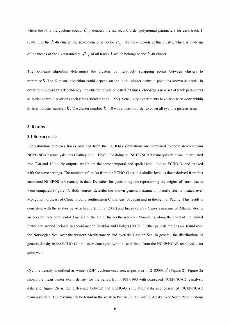
6
where the N is the cyclone count, ji , denotes the six second order polynomial parameters for each track i
(L=6). For the k -th cluster, the six-dimensional vector jk , are the centroids of this cluster, which is made up
of the means of the six parameters ji, of all tracks i which belongs to the k -th cluster.
The K-means algorithm determines the clusters by iteratively swapping points between clusters to
minimize S .The K-means algorithm could depend on the initial cluster centroid positions known as seeds. In
order to minimize this dependency, the clustering was repeated 20 times, choosing a new set of track parameters
as initial centroid positions each time (Blender et al. 1997). Sensitivity experiments have also been done within
different cluster numbers k . The cluster number k =10 was chosen in order to cover all cyclone genesis areas.
3. Results
3.1 Storm tracks
For validation purposes tracks obtained from the ECHO-G simulations are compared to those derived from
NCEP/NCAR reanalysis data (Kalnay et al., 1996). For doing so, NCEP/NCAR reanalysis data was interpolated
into T30 and 12 hourly outputs, which are the same temporal and spatial resolution as ECHO-G, and tracked
with the same settings. The numbers of tracks from the ECHO-G are at a similar level as those derived from this
coarsened NCEP/NCAR reanalysis data. Densities for genesis regions representing the origins of storm tracks
were compared (Figure 1). Both sources describe the known genesis maxima for Pacific storms located over
Mongolia, northeast of China, around southeastern China, east of Japan and in the central Pacific. This result is
consistent with the studies by Adachi and Kimura (2007) and Inatsu (2009). Genesis maxima of Atlantic storms
are located over continental America in the lee of the northern Rocky Mountains, along the coast of the United
States and around Iceland, in accordance to Hoskins and Hodges (2002). Further genesis regions are found over
the Norwegian Sea, over the western Mediterranean and over the Caspian Sea. In general, the distributions of
genesis density in the ECHO-G simulation data agree with those derived from the NCEP/NCAR reanalysis data
quite well.
Cyclone density is defined as winter (DJF) cyclone occurrences per area of 218000km2 (Figure 2). Figure 2a
shows the mean winter storm density for the period from 1951-1990 with coarsened NCEP/NCAR reanalysis
data and figure 2b is the difference between the ECHO-G simulation data and coarsened NCEP/NCAR
reanalysis data. The maxima can be found in the western Pacific, in the Gulf of Alaska over North Pacific, along

7
the coast of North America, in the southeast of Greenland and Barents Sea. For ECHO-G simulation data, the
cyclone density over the Gulf of Alaska, in the south of Greenland, and Western Europe is larger, while it is
smaller in southeast China, over the east of Japan and in the western Mediterranean Sea (Figure 2b). But the
differences are not large and the cyclone density pattern agrees with other results (Gulev et al. 2001, Hoskins and
Hodges 2002). So we conclude that the midlatitude cyclone statistics generated from the ECHO-G simulation
data are realistic.
The 990-year time series of winter cyclone numbers for the NH are shown in Figure 3. Average cyclone numbers
in each century are shown in Figure 4. The smallest average cyclone number of 179/yr is in the twentieth century
(1900-1990). Also in the thirteenth (1201-1300) and fourteenth (1301-1400) century relatively few storms are
counted, with 180 per year. Highest numbers (182 counts per year) emerge in the fifteenth (1401-1500) century.
But generally the average cyclone frequency for different centuries is quite similar with little variability and
decoupled from temperature (Figure 4), while the year-to-year variations for storm numbers are strong (Figure
3). Long-term trends can not be detected during the quasi-millennial winters of years1001-1990.
This result is very similar to that of Fischer-Bruns et al. (2005) who used the maximum wind speed to define
storm days based on a shorter ECHO-G simulation. They compared the storm day frequency between pre-
industrial times (1551-1850) and industrial times (1851-1990) and found no noticeable differences. They stated
that during historical times storms statistics for both hemisphere are remarkably stable with little variability and
storminess mostly decoupled from temperature variations. Only in the climate change scenarios, which describe
possible developments in the 21st century, with a strong increase of greenhouse gas concentrations, the
distributions of high storm frequency exhibited a poleward shift. But there is no increase in the number of storms
when the sum over the entire Northern Hemisphere is formed.
However, compared to higher resolution, the track numbers derived from coarse temporal and spatial grids are
underestimated (Blender and Schubert 2000, Jung et al. 2006, Zolina and Gulev 2002). According to the study of
Jung et al. (2006), cyclones in the northern Pacific, the Arctic, Baffin Bay, the Labrador Sea and the
Mediterranean Sea are specifically sensitive to the spatial resolution. Our results differ from what has been
reported by Gulev et al. (2001) – the cyclone density of ECHO-G is up to 12 cyclones per winter per 218000 km2
(Figure 2) which is less than the number given by Gulev et al. (2001) (up to 20 cyclones per winter per 218000
km2). This difference may partly be due to the different resolution or other deficits of the model ECHO-G, but it

8
may also reflect different tracking settings of these two studies in determining storm tracks. More important is
that the overall patterns and the relative frequencies are comparable.
3.2 Clustering results
All tracks were clustered into ten groups by applying the K-means method in each century (Figure 5). The
centroid track is the mean track of each cluster. We can see that the 10 clusters form a kind of midlatitude ring
around the Northern Hemisphere (Figure 5), with a poleward bend at their ends. It is similar to the schematic of
principal tracks (Figure 15 of Hoskins and Hodges, 2002) and consistent with the genesis areas (Figure 1).
Across the Pacific, tracks are separated into three clusters: cluster 4 from the southeast of China to the Japan Sea,
cluster 5 from the east of Japan to the center of the Pacific, and cluster 6 in the eastern Pacific. In the Atlantic,
there are also 3 clusters: cluster 8 from the eastern North American coast, cluster 9 from the southern Greenland,
and cluster 10 extending from southeastern Iceland to the Norwegian Sea. Cluster 7 corresponds to the tracks
generated from continental American in the lee of the northern Rocky Mountains. The classifications in the
Pacific and Atlantic are quite similar to those of Gulev et al. (2001) except that only two clusters appear for the
Pacific.
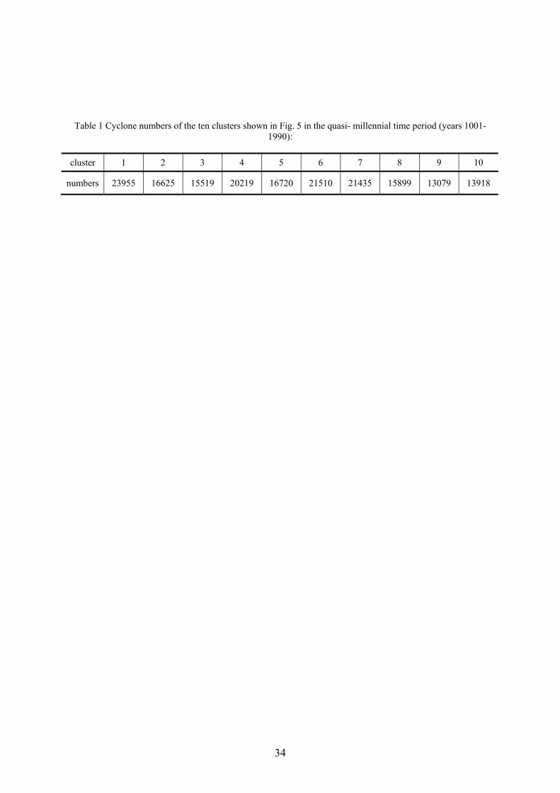
Table 1 lists the numbers of tracks per cluster for the whole time period 1001-1990. Cluster 1 which emanates
from the North Sea, Baltic Sea and the western Mediterranean has the most members. In the Pacific, the eastern
cluster 6 has the highest numbers of tracks, while the central cluster 5 has the fewest. Over the Atlantic, the
western cluster 8 has the most tracks, whereas the fewest number is found in the central cluster 9. The sum of
cyclone counts for the three Pacific clusters (4, 5, 6) is larger than that for the three Atlantic clusters (8, 9, 10).
Many studies found tracks or track density shift northward in the future greenhouse gas forcing (Schubert et al.
1998, Ulbrich and Christoph 1999, Fischer-Bruns et al. 2005, and Pinto et al. 2007). Observation from satellite
also supports that the storm cloudiness has a poleward shift (Bender et al. 2012). Figure 6 displays the centroid
(mean) tracks of the ten clusters for the earliest 11th century (years 1001-1100) and the latest 20th century (years
1900-1990). They differ very little. Obviously, the geometric positions of the tracks were quite similar in the first
and last century of the last millennium. The results of Fischer-Bruns et al. (2005) indicate that it is not the
hemispheric temperature, which is related to the change in tracks, but other factors, such as the zone of
maximum baroclinicity.
9
Figure 7 shows the average cyclone numbers for the 10 clusters in different centuries. There are no large
variations between different centuries; the large differences in cyclone counts between the clusters vary very
little from century to century. Some may expect systematic changes, at least over the North Atlantic for
centuries, when regional significant temperature anomalies prevail, such as the Medieval Warm Period (AD 950-
1250) and the Little Ice Age (AD 1500-1700) (Keigwin 1996, KIHZ-Consortium 2004) -- however, the
differences are rather small (Figure 7: cluster 8, 9 and 10). Fischer-Bruns et al. (2005) stated that the variations
of storm activity are not linearly related to temperature variability during historical times in the ECHO-G
simulation.
Table 2 shows the distribution of lifetimes for all clusters. Overall, the highest percentage is found for the
lifetimes of 2-4 days. For clusters 2, 3 and 6 over 60% of tracks last 2-4 days. Cluster 8, primarily located over
the eastern North American coast, contains most long-lived (more than 10 days) cyclones with about 7% of all its
cyclones (Table 2 and Figure 8 b). Over the Atlantic, the eastern cluster 10 which extends from southeastern
Iceland to the Norwegian Sea, shows an average lifetime of about 5 days; also the number of long-lived cyclones
(5.0%) is a little larger than cluster 9. For the Pacific, cluster 4 has the highest percentage (5.6%) of cyclones
lasting more than 10 days with a mean lifetime of about 6 days (Figure 8 a). In general, cyclones travelling from
land to the sea tend to exist for a longer time, such as those in clusters 3 and 7. The warm Kuroshio current in the
Pacific and the Gulf stream in the Atlantic play important roles in generating baroclinic situations favoring the
lasting of cyclones. Latent heat release and moisture over the ocean also contribute to the development of
cyclones and make them survive longer.
Deepening rates for each track were determined, and frequency distributions for these rates for all tracks in a
cluster derived. The “averaged” deepening rate is calculated for the period, from genesis location to the
maximum pressure value; the “maximum” deepening rate” is the largest pressure fall along a track. Table 3
shows the mean deepening rates per 12 hours for the ten clusters for the whole time period 1001-1990. In the
Atlantic, the average deepening rates are mainly between 2-4 hPa/12h for clusters 8, 9, and 10 with 38.2%,
38.4% and 45.0%, respectively (Figure 8 d and Table 3). Cluster 8 for the eastern North American coast also
shows an elevated average deepening rate of 4-6 hPa/12h. In the Pacific, there are more cyclones with an average
deepening rate of 4-6 hPa/12h compared with Atlantic cyclones: especially cluster 4 in the western Pacific
(30.7%, Figure 8 c). In other clusters average deepening rates are mostly about 0-2 hPa/12h, except for clusters 1
and 7 which have their largest deepening rate percentage between 2 to 4 hPa per 12 hours (Table 3).

10
Table 4 lists the distributions of maximum deepening rates per 12 hours. Figure 8 e and f show maximum
deepening rates for the Pacific and the Atlantic. In the Pacific, more than about 25% of all cyclones go with a
rapid maximum deepening rate of more than 10hPa/12h. Cluster 5 over the central Pacific has the highest
maximum deepening rate (36.6%) of more than 10 hPa per 12h (Figure 8 e). Over the Atlantic, the maximum
deepening rates of more than 10 hPa per 12h occur less often than over the Pacific. Only cluster 8 over the
eastern North American coast shows a maximum deepening rate over 10 hPa per 12h for 23.4% of all its
cyclones (Figure 8 f). Cluster 9 (22.2%) over southern Greenland, and cluster 10 (26.9%), extending from
southeastern Iceland to the Norwegian Sea, show mainly maximum deepening rates of 4-6 hPa/12h. From the
studies of Gulev et al. (2001) of NCEP/NCAR re-analysis and from Uccellini (1990) it is known that the largest
deepening takes place over the oceans. Thus, the statistics of the ECHO-G cyclone clusters are found to be
consistent with the previous analysis of “observed” cyclone activity.
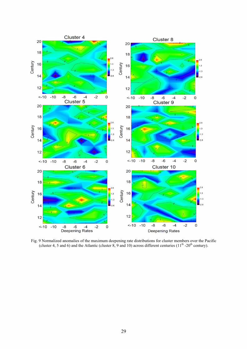
Figure 9 shows changes of the maximum deepening rates for the Atlantic and Pacific clusters during different
centuries. In the 20th century maximum deepening rates larger than 10 hPa per 12h become less frequent for
cluster 8 but more frequent for cluster 10 in the Atlantic (Figure 9 right). Between the 17th and 18th century the
maximum deepening rates for cluster 8 of 6-8 hPa per 12h become more frequent, but those larger than 8 hPa per
12h less frequent. There are tendencies of decreases in the frequency of deep cyclones in the 16th-17th and 19th
century for cluster 9 and in the 16th and 19th century for cluster 10. In the Pacific, in the 20th century frequencies
of rapidly deepening cyclones (over 10 hPa/12h) slightly increase for cluster 4 and 5 (Figure 9 left), and
relatively slowly deepening cyclones (2-4 hPa/12h) appear more often in cluster 4 but less so in cluster 6. There
are decreases in the frequency of deep cyclones in the 11th and 19th century for cluster 4, during the15th to 16th
century for cluster 5, and in the 12th century and during the 14th to 16th century for cluster 6.
3.3 Interactions between clusters
Linkages between cyclonic activities in the Pacific and the Atlantic have been studied before (May and
Bengtsson 1998, Sickmöller et al. 2000). Sickmöller et al. (2000) showed that the numbers of the north-eastward
direction cyclones in the Pacific are related to the frequency of the north-eastward and zonal directional cyclones
in the Atlantic. It was also suggested that upper-level Pacific depressions could cross North America and
influence the genesis of cyclones over the western Atlantic.

11
We analyzed the correlations of the numbers between the ten clusters (Table 5), as derived from all 990 winters
of the simulation. The main feature is a significant, albeit not large negative correlation between neighboring
clusters, e.g., between the Atlantic clusters 8 and 9 (-0.23), the Pacific clusters 4/5 (-0.22) and 5/6 (-0.32), the
continental clusters 7/8 (-0.22) and 1/10 (-0.21). Also minor correlations are found between non-neighboring
clusters across the North American continent such as clusters 6/8 (-0.12), 6/9 (0.13), and 6/10 (0.11). Thus the
linkage between neighboring clusters is not strong but a robust feature, while the remote linkages are very weak.
3.4 Links to large-scale pressure patterns
We investigate how seasonal (DJF) mean MSLP patterns are related to the yearly numbers of cyclones in the
Pacific and the Atlantic. Canonical Correlation Analysis (CCA) (von Storch and Zwiers 1999) is used to
determine systematic mutual dependencies in the yearly MSLP fields and yearly cyclone counts for the three
clusters in the Pacific and the Atlantic separately. Prior to the CCA, a data compression was done truncating the
high-dimensional MSLP fields to the first thirteen Empirical Orthogonal Functions (EOFs) (von Storch and
Zwiers 1999). The fields, both EOF-truncated MSLP as well as cluster counts, are based on deviations from the
long-term (990 winters) mean, i.e. anomalies.
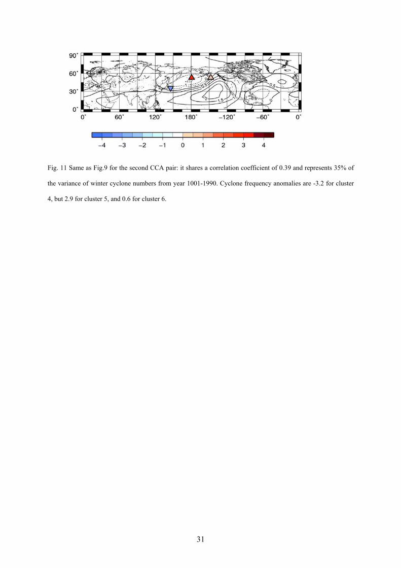
Figures 10 and 11 show the two most important related patterns linking MSLP and cyclone frequency anomalies
in the Pacific. The coefficient time series of the first (second) CCA pattern have a correlation of about 0.6 (0.4)
and the pattern describes 48% (35%) of the variance of winter cyclone counts in the Pacific.
The first Pacific pattern (Figure 10) is a unipolar pressure pattern with a center around the Aleutian Islands with
minimum values below over -4.5 hPa. When the CCA coefficient is 1, then the maximum yearly mean Aleutian
pressure anomaly is more than -4.5 hPa, the number of cyclones in cluster 4 is decreased by -0.6, in cluster 5
decreased by – 2.2 and increased in cluster 6 by 4.6, on average. Thus, when the CCA pattern has a positive
coefficient, the Aleutian Low tends to be stronger (lower pressure) and cyclone numbers of the eastern cluster 6
increase whereas cyclone counts in the western (cluster 4) and central (cluster 5) Pacific tend to be lower.
The second Pacific pattern (Figure 11) describes a bipolar pressure pattern between the Aleutian Islands and
North America with a pressure contrast of more than 3 hPa. This relates to a decrease/increase of cyclone counts
in the western Pacific (cluster 4) but increase/decrease in the central (cluster 5) and eastern Pacific (cluster 6).
This pattern seems to be related to the Pacific North American Oscillation (PNA) pattern, albeit with a shift,

12
which is associated with the East Asian jet stream and influences cyclone genesis in the eastern Pacific
(Sickmöller et al. 2000, Gulev et al. 2001) and cyclone activity in the western Atlantic (Christoph and Ulbrich
2000).
Figure 12 and 13 are the first and second CCA patterns for clusters 8, 9 and 10 over the Atlantic. The first pattern
has a correlation of 0.5 for the coefficient time series and the second pattern shares a correlation of 0.3. They
present about 39% and 31%, respectively, of the variance for the year-to-year winter cyclone counts.
The first Atlantic pattern (Figure 12) is a dipole located over the Iceland Low areas and the Atlantic subtropics
with a pressure contrast of more than 4 hPa obviously related to the North Atlantic Oscillation (NAO) pattern
with deeper/higher Iceland low and higher/shallower subtropical high. In the positive phase (deeper Icelandic
Low) there are more cyclones for cluster 9 and cluster 10 over the southeast of Greenland and northeastern
Atlantic, which agree with the study of Sickmöller et al. (2000). The NAO is known to be associated with
variations of storm activity over the North Atlantic (Ulbrich and Chirstoph 1999, Sickmöller et al. 2000, Gulev et
al. 2001, Pinto et al. 2007 and Raible et al. 2007). When the NAO is in its positive phase, cold air from Arctic
areas is encountering the warm North Atlantic current, and baroclinicity increases over the north Atlantic. This
leads to more cyclone activity over the northeastern Atlantic. When the NAO is in its negative phase with a
shallower Icelandic Low, cyclones shift southward and more intense cyclones happen in the Mediterranean area
(Raible et al. 2007).
The second Atlantic pattern (Figure 13) shows a unipolar pattern located over the Atlantic with values of more
than -2.5 hPa. It relates that more cyclones show up along the eastern North Atlantic (cluster 10). And there are
fewer cyclones over the coast of America (cluster 8) and over southern Greenland (cluster 9).
4. Conclusions
A coupled global atmosphere-ocean model (ECHO-G) simulation for the last about one thousand years was
analyzed for changes in winter storm activity. The ECHO-G model was exposed to realistic variations of
shortwave solar input, time-dependent presence of volcanic material in the upper atmosphere, and slowly
changing greenhouse gas concentrations during the last millennium 1000-1990. An automatic tracking algorithm
(Hodges 1994, 1995, and 1999) was used to locate extratropical cyclones within the simulated MSLP fields. For
validation reasons, the tracks were also compared with coarsened NCEP/NCAR reanalysis data. The main result

13
of the study is that the time series of cyclone counts for years 1001 to 1990 show strong year to year variations,
but an obvious trend was not found.
Tracks were clustered into ten groups by applying the K-means method. The cluster results mainly correspond to
the cyclone genesis areas. Frequency and distributions of lifetime as well as deepening rates were studied for the
ten clusters. The oceanic cyclones show rapid deepening rates and a relatively long lifetime. Storm tracks in the
Pacific are clustered into three groups: tracks over the western Pacific, in the central Pacific and in the eastern
Pacific. In the Atlantic, tracks are also grouped into three clusters: tracks are located over the eastern North
American coast, southern Greenland, and southeastern Iceland and the Norwegian Sea. The frequencies of
cyclones in these two oceans are connected to large-scale pressure patterns. The main results for the Pacific and
the Atlantic are concluded as follows:
The Pacific: Most cyclones are in the eastern Pacific, but fewest are in the central Pacific. Cyclones in the
western Pacific survive longest (average lifetime of 6 days) and also show the highest percentage of cyclones
lasting more than 10 days. Cyclones of the central Pacific have the highest proportions to deepen rapidly (>10
hPa per 12h). In the 20th century those cyclones that deepen rapidly (> 10hPa per 12h) become slightly more
frequent over the western and central Pacific. Frequencies of cyclones over the western, central and eastern
Pacific are correlated with each other and are also related to the Aleutian Low. When the Aleutian Low is
stronger, cyclones in the eastern Pacific increase. Cyclones in the eastern Pacific show weak teleconnections
across the American continent with cyclones in the Atlantic.
The Atlantic: Cyclones located over the eastern North American coast show the highest total numbers, the
longest lifetimes with an average lifespan of 6 days, and also most cyclones which deepen rapidly (>10 hPa per
12h) occur in this region. In the 20th century those rapidly deepening cyclones become less frequent over the
eastern North American coast, but more frequent over southeastern Iceland and the Norwegian Sea. Cyclone
counts over the Atlantic are correlated to the NAO pattern. During the positive NAO phase, there are more
cyclones over the southeast of Greenland, the northeastern Atlantic and northwest Europe. Cyclone numbers
over the Atlantic are smaller than for the Pacific. And more cyclones over the Pacific than over the Atlantic show
a strong deepening rate of at least 10hPa/12h.

14
We conclude that this simulation of the last millennium shows only smaller variations on decadal to centennial
time scales and no long-term trends for the whole period. This is valid for the location and numbers of cyclone
tracks which are changing only marginally.
There are a number of caveats: First, the data are generated by a model as a response to prescribed, estimated
external forcing (solar, volcanic material, greenhouse gases). These estimated external forcing factors may
deviate from reality –as discussions so far point more to an overestimation of solar and volcanic factors. If that
would be so, then the conclusions of “little centennial variations of storm track statistics” would not be affected.
Also the model may show too small variations of storm activity, in particular related to the coarse spatial
resolution of only T30. Comparison with other studies indicates that there may be an underestimate, but this
would be stationary in time, so that our conclusion about temporal variability would not be affected. Finally, the
relatively infrequent storing of MSLP fields, only once in every 12 hours, may have lead to too few detectable
storms. We consider this possibility also less relevant, first because of successful previous studies with this
“coarse” gridding. And again such a bias would hardly affect the strength of variations. But all in all, these
caveats must be acknowledged, and future studies of similar millennial simulations, with better horizontal and
temporal gridding, will show their significance.
Acknowledgments: We thank Eduardo Zorita for providing ECHO-G simulation data, his support with statistic routines,
and helpful discussions. We appreciate Kevin I. Hodges help with his tracking algorithm which was used for our study. The
NCEP/NCAR reanalysis data were provided by the National Centre for Atmospheric Research (NCAR). We thank Beate
Geyer for providing the NCEP/NCAR reanalysis data and technical supports. We also thank Beate Gardeike for her help to
prepare the figures. This work was funded by the China Scholarship Council (CSC) and the Institute of Coastal Research
Helmholtz-Zentrum Geesthacht within the framework of the Junior Scientist Exchange Program organised by the CSC and
the Helmholtz Association of German research centres (HGF). This work is a contribution to the “Helmholtz Climate
Initiative REKLIM” (Regional Climate Change), a joint research project of HGF. The authors thank two anonymous
reviewers for constructive comments that helped to improve this article.

15
Reference Adachi S. and F. Kimura, 2007: A 36-year climatology of surface cyclogenesis in East Asia using high-resolution reanalysis
data. Sola, 3, 113-116.
Alexandersson H, T. Schmith, K. Iden, and H. Tuomenvirta, 1998: Longterm variations of the storm climate over NW
Europe. Global Atmosphere Ocean System, 6, 97–120.
Bengtsson L. and K. I. Hodges, 2006: Storm tracks and climate change. Journal of Climate, 19, 3518-3543.
Bender F. A-M., V. Ramanathan, G. Tselioudis, 2012: Changes in extratropical storm track cloudiness 1983-2008:
Observation support for a poleward shift. Climate Dynamics, 38, 2037-2053.
Blender R., K. Fraedrich and F. Lunkeit, 1997: Identification of cyclone-track regimes in the North Atlantic. Quarterly
Journal of the Royal Meteorological Society, 123, 727-741.
Blender R. and M. Schubert, 2000: Cyclone tracking in different spatial and temporal resolutions. Monthly Weather Review,
128, 377-384.
Brayshaw D. J., B. Hoskin, and M. Blackburn, 2008: The storm-track response to idealized SST perturbations in an
aquaplanet GCM. Journal of Atmospheric Sciences, 65, 2842-2860.
Christoph M. and U. Ulbrich, 2000: Can NAO-PNA relationship be established via the North Atlantic storm track?
Geophysical Research Abstracts, 2, 215.
Chu P., X. Zhao and J. Kim, 2010: Regional typhoon activity as revealed by track patterns and climate change. Hurricanes
and Climate Change, 2, 137-148.
Elsner J. B., K.-b. Liu, and B. Kocher, 2000: Spatial variations in major U.S. hurricane activity: Statistics and a physical
mechanism. Journal of Climate, 13, 2293–2305.
Elsner J. B., 2003: Tracking hurricanes. Bulletin of the American Meteorological Society, 84, 353-356.
Fischer-Bruns I, H. von Storch, J. F. González-Rouco and E. Zorita, 2005: Modelling the variablility of midlatitude storm
activity on decadal to century time scales. Climate Dynamics, 25(5), 461-476.

16
González-Rouco F., H. von Storch, and E. Zorita, 2003: Deep soil temperature as proxy for surface air-temperature in a
coupled model simulation of the last thousand years. Geophysical Research Letters, 30(21), 2116.
Gouirand I., V. Moron, and E. Zorita, 2007: Teleconnections between ENSO and North Atlantic in an ECHO-G simulation of
the 1000-1990 period. Geophysical Research Letters, 34, L06705.
Gulev S. K., O. Zolina and S. Grigoriev, 2001: Extratropical cyclone varibility in the Northern Hemisphere winter from the
NCEP/NCAR reanalysis data. Climate Dynamics, 17, 795-809.
Hodges K. I., 1994: A general method for tracking analysis and its application to meteorological data. Monthly Weather
Review, 122, 2573-2586.
Hodges K. I., 1995: Feature tracking on the unit sphere. Monthly Weather Review, 123, 3458-3465.
Hodges K. I., 1999: Adaptive constraints for feature tracking. Monthly Weather Review, 127, 1362-1373.
Hoskins B. J. and K. I. Hodges, 2002: New perspectives on the Northern Hemisphere winter storm tracks. Journal of the
Atmospheric Sciences, 59, 1041-1061.
Hoskins B. J. and K. I. Hodges, 2005: A new perspective on Southern Hemisphere storm tracks. Journal of Climate, 18,
4108-4129.
Hurrell J. W., 1995: Decadal trends in the North Atlantic Oscillation: regional temperatures and precipitation. Science, 269,
676-679.
International Detection and Attribution Group (IDAG), 2005: Detecting and attributing external influences on the climate
system: A review of recent advances. Journal of Climate, 18, 1291-1314.
Inatsu M., 2009: The neighbor enclosed area tracking algorithm for extratropical wintertime cyclones.
Atmospheric Science Letters, 10, 267-272.
Jung T., S. K. Gulev, I. Rudeva and V. Soloviov, 2006: Sensitivity of extratropical cyclone characteristic to horizontal
resolution in ECMWF model. Quarterly Journal of the Royal Meteorological Society, 132, 1839-1857.

17
Kalnay, E., Kanamitsu, M., Kistler, R., Collins, W., Deaven, D. and co-authors. 1996. The NCEP/NCAR 40-year reanalysis
project. Bulletin of the American Meteorological Society, 77, 437–471.
Keigwin L. D., 1996: The Little Ice Age and Medieval Warm Period in the Sargasso Sea. Science, 274, 1503-1508.
KIHZ-Consortium: Zinke J., H. von Storch, B. Müller, E. Zorita, B. Rein, H. B. Mieding, H. Miller, A. Lücke, G.H. Schleser,
M.J. Schwab, J.F.W. Negendank, U. Kienel, J.F. González-Rouco, C. Dullo and A. Eisenhauser, 2004: Evidence for the
climate during the Late Maunder Minimum from proxy data available within KIHZ. In Fischer H., T. Kumke, G. Lohmann,
G. Flöser, H. Miller, H von Storch and J. F. W. Negendank (Eds.): The Climate in Historical Times. Towards a synthesis of
Holocene proxy data and climate models, Springer, Berlin - Heidelberg - New York, 487 pp., ISBN 3-540-20601-9, 397-414.
Matulla C., W. Schöner, H. Alexandersson, H. von Storch, and X. L. Wang, 2008: European storminess: late nineteenth
century to present. Climate Dynamics, 31,125–130.
May W. and L. Bengtsson, 1998: The signature of ENSO in the Northern Hemisphere midlatitude season mean flow and
high-frequency intraseasonal variability. Meteorology and Atmospheric Physics, 69, 81-100.
Min S. K., S. Legutke, A. Hense, and W. T. Kwon, 2005 a: Internal variability in a 1000-yr control simulation with the
coupled climate model ECHO-G. I: Near-surface temperature, precipitation and mean sea level pressure, Tellus A, 57, 605-
621.
Min S. K., S. Legutke, A. Hense, and W. T. Kwon, 2005 b: Internal variability in a 1000-yr control simulation with the
coupled climate model ECHO-G. II: El Niño Southern Oscillation and North Atlantic Oscillation, Tellus A, 57, 622-640.
Moberg A., D. M. Sonechkin, K. Holmgren, N. M. Datsenko and W. Karlén, 2005: Highly variable Northern Hemisphere
temperatures reconstructed from low- and high-resolution proxy data, Nature, 433, 613-617.
Murray R. J. and I. Simmonds, 1991: A numerical scheme for tracking cyclone centres from digital data Part I: development
and operation of the scheme. Australian Meteorological Magazine, 39, 155-166.
Muskulus M. and D. Jacob, 2005: Tracking cyclones in regional model data: the future of Mediterranean storms. Advanced
Geosciences, 2, 13-19.

18
Nakamura J., U. Lall, Y. Kushnir and S. J. Camargo, 2009: Classifying North Atlantic tropical cyclone tracks by mass
moments. Journal of Climate, 15, 5481-5494.
Pinto J. G., U. Ulbrich, G. C. Leckebusch, T. Spangehl, M. Reyers, and S. Zacharias, 2007: Changes in storm track and
cyclone activity in three SRES ensemble experiments with the ECHAM5/MPI-OM1 GCM. Climate Dynamics, 29, 195-210.
Raible C. C. and R. Blender, 2004: Northern Hemisphere Mid-latitude cyclone variability in different ocean representations.
Climate Dynamics, 22, 239-248.
Raible C. C., M. Yoshimori, T. F. Stocker and C. Casty, 2007: Extreme midlatitude cyclones and their implications for
precipitation and wind speed extremes in simulations of the Maunder Minimum versus present day conditions. Climate
Dynamics, 28, 409-423.
Roeckner E., K. Arpe, L. Bengtsson, M. Christoph, M. Claussen, L. Dümenil, M. Esch, M. Giorgetta, U. Schlese, and U.
Schulzweida, 1996: The atmopheric general circulation model ECHAM4: model description and simulation of present-day
climate. Report No. 218, 90 pp, Max-Planck-Institut für Meteorologie, Bundesstr 55, Hamburg.
Rudeva I. and S. K. Gulev, 2007: Climatology of cyclone size characteristic and their changes during the cyclone life cycle.
Monthly Weather Review, 135, 2568-2587.
Schubert M., J. Perlwitz, R. Blender, K. Fraedrich and F. Lunkeit, 1998: North Atlantic cyclones in CO2-induced warm
climate simulations: frequency, intensity and tracks. Climate Dynamics, 14, 827-837.
Serreze M. C. 1995: Climatological aspects of cyclone development and decay in the arctic. Atmosphere- Ocean, 33(1), 1-23.
Sickmöller M., R. Blender and K. Fraedrich, 2000: Observed winter cyclone tracks in the northern hemisphere in re-analysed
ECMWF data. Quarterly Journal of the Royal Meteorological Society, 126, 591-620.
Stendel M. and E. Roeckner, 1998: Impacts of horizontal resolution on simulated climate statistics in ECHAM4. Report No.
253, Max-Planck-Institut für Meteorologie, Bundesstr 55, Hamburg.
Tan M., X. Shao, J. Liu and B. Cai, 2009: Comparative analysis between a proxy-based climate reconstruction and GCM-
based simulation of temperature over the last millennium in China. Journal of Quaternary Science, 24(5), 547-551.

19
Uccellini L. W., 1990: Process contributing to the rapid development of extratropical cyclones. In: Newton CW, Holopainen
EO (eds) Extratropical cyclones. The Eric Palmen memorial volume. AMS, Boston, 81-106.
Ulbrich U. and M. Christoph, 1999: A shift of the NAO and increasing storm track activity over Europe due to anthropogenic
greenhouse gas forcing. Climate Dynamics, 15, 551-559.
Ulbrich U., G. C. Leckebusch and J. G. Pinto, 2009: Extra-tropical cyclones in the present and future climate: a review.
Theoretical and Applied Climatology, 96, 117-131.
von Storch, J.-S., V. Kharin, U. Cubasch, G. Hegerl, D. Schriever, H. von Storch, E. Zorita, 1997: A 1260 year control
integration with the coupled ECHAM1/LSG general circulation model. Journal of Climate, 10, 1526-154.
von Storch and F. W. Zwiers, 1999: Statistical analysis in climate research. Cambridge University Press, Cambridge, UK,
503pp.
von Storch H., E. Zorita, Y. Dimitriev, F. González-Rouco, and S. Tett, 2004: Reconstructing past climate from noisy data.
Science, 306, 679-682.
Weisse, R., H. von Storch, and F. Feser, 2005: Northeast Atlantic and North Sea Storminess as Simulated by a Regional
Climate Model during 1958-2001 and Comparison with Observations. Journal of Climate, 18(3), 465-479.
Wernli H. and C. Schwierz, 2006: Surface cyclones in the ERA-40 dataset (1958-2001). Part I: novel identification method
and global climatology. Journal of the Atmospheric Sciences, 63, 2486-2507.
Wolff J. O., E. Maier-Reimer, and S. Legutke, 1997: The Hamburg Ocean primitive equation model. Technical Report, No.
13, 98 pp, German Climate Computer Center (DKRZ), Hamburg.
Xia L., M. Zahn, K. I. Hodges, F. Feser, and H. von Storch, 2012: A comparison of two identification and tracking Methods
for polar lows. Tellus A, 64, 17196.
Zahn M. and H. von Storch, 2008a: Tracking polar lows in CLM. Meteorologische Zeitschrift, 17(4), 445-453.
Zahn M. and H. von Storch, 2008b: A long-term climatology of North Atlantic polar lows. Geophysical Research Letters, 35,
L22702.

20
Zolina O. and S. K. Gulev, 2002: Improving the accuracy of mapping cyclone numbers and frequencies. Monthly Weather
Review, 130, 748-759.
Zorita E., J. F. González-Rouco, H. von Storch, J. P. Montávez, and F. Valero, 2005: Natural and anthoropogenic model of
surface temperature variations in the last thousand years. Geophysical Research Letters, 32, L08707.

21
Fig. 1 40-years (1951-1990) average density distribution of cyclone genesis in winter for the Northern
Hemisphere: (a) coarsened NCEP/NCAR reanalysis data; (b) ECHO-G simulation data.

22
Fig. 2 40-years (1951-1990) mean cyclone density (unit: cyclones/winter per 218000km2) for the Northern Hemisphere: (a) coarsened NCEP/NCAR reanalysis data; (b) difference between ECHO-G simulation data and coarsened NCEP/NCAR reanalysis data.

23
Fig. 3 Time series of the numbers of winter (DJF) extratropical cyclones (black line) and winter surface air
temperature (SAT: K) (red line) in the Northern Hemisphere (NH) (years 1001-1990).

24
Fig. 4 Average annual numbers of winter (DJF) extratropical cyclones (black line) and average winter SAT (K)
(red line) in the NH for different centuries (11th -20th century).

25
Fig. 5 Winter (DJF) extratropical cyclone tracks of the 20th century (years 1900-1990) in the NH clustered into
ten clusters by applying the K-means method: member tracks (blue) and centroid tracks (red) of the ten clusters.

26
Fig. 6 Mean tracks of ten clusters (red numbers) for the NH in the 11th and 20th century: red ones are the mean tracks of the ten clusters in the11th century (years 1001-1100), blue ones with circles are the mean tracks of the
ten clusters in the 20th century (years 1901-1990).

27
Fig. 7 Average annual numbers of winter (DJF) extratropical cyclones in the NH for the ten clusters in different
centuries (11th - 20th century).

28
Fig. 8 Distributions (%) of cyclone lifetime (days) (a and b), mean deepening rates (hPa/12h) (c and d), and
maximum deepening rates (hPa/12h) (e and f) for winter cyclones over the Pacific (a, c and e) and the Atlantic (b, d and f) for the whole time period (years 1001-1990).
(a) (b)
(c) (d)
(e) (f)
29
Fig. 9 Normalized anomalies of the maximum deepening rate distributions for cluster members over the Pacific (cluster 4, 5 and 6) and the Atlantic (cluster 8, 9 and 10) across different centuries (11th -20th century).
30
Fig.10 Corresponding correlation patterns between time series of winter (DJF) cyclone numbers in the Pacific
(clusters 4, 5 and 6) (triangles: for positive values, for negative values) and mean sea level pressure
fields in hPa (isolines: dashed for negative and solid for positive). The first CCA pair shares a correlation
coefficient of 0.59 and represents 48% of the variance of winter cyclone numbers from year 1001-1990. Cyclone
frequency anomalies are -0.6 for cluster 4, -2.2 for cluster 5, but 4.6 for cluster 6.
31
Fig. 11 Same as Fig.9 for the second CCA pair: it shares a correlation coefficient of 0.39 and represents 35% of
the variance of winter cyclone numbers from year 1001-1990. Cyclone frequency anomalies are -3.2 for cluster
4, but 2.9 for cluster 5, and 0.6 for cluster 6.

32
Fig.12 Corresponding correlation patterns between time series of winter (DJF) cyclone numbers in the Atlantic
(clusters 8, 9 and 10) (triangles: for positive values, for negative values) and mean sea level pressure
fields in hPa (isolines: dashed for negative and solid for positive). The first CCA pair shares a correlation
coefficient of 0.51 and represents 39% of the variance of winter cyclone numbers from year 1001-1990. Cyclone
frequency anomalies are -0.9 for cluster 8, but 3.0 for cluster 9, and 2.0 for cluster 10.

33
Fig. 13 Same as Fig.11 for the second CCA pair: it shares a correlation coefficient of 0.27 and represents 31% of
the variance of winter cyclone numbers from year 1001-1990. Cyclone frequency anomalies are -1.7 for cluster 8
and -1.7 for cluster 9, but 2.3 for cluster 10.
34
Table 1 Cyclone numbers of the ten clusters shown in Fig. 5 in the quasi- millennial time period (years 1001-1990):
cluster 1 2 3 4 5 6 7 8 9 10
numbers 23955 16625 15519 20219 16720 21510 21435 15899 13079 13918

35
Table 2 Lifespan (days) distribution rates of the ten clusters shown in Fig. 5 in the quasi- millennial time period
(years 1001-1990). Unit: %:
lifetime(days) 2~4 4~6 6~8 8~10 >10 Cluster 1 43.25 30.20 16.70 6.19 3.65 Cluster 2 60.82 25.86 7.99 3.04 2.29 Cluster 3 63.12 15.11 10.02 6.60 5.15 Cluster 4 36.02 28.98 19.96 9.40 5.64 Cluster 5 50.19 29.93 12.40 4.45 3.03 Cluster 6 60.38 24.42 8.51 3.84 2.86 Cluster 7 56.66 18.03 13.28 6.80 5.23 Cluster 8 39.10 29.74 16.48 7.72 6.96 Cluster 9 55.68 23.62 10.54 5.25 4.92
Cluster 10 47.96 24.68 14.59 7.77 5.01

36
Table 3 Mean deepening rate (hPa/12h) distributions of the ten clusters shown in Fig. 5 in the quasi- millennial time period (years 1001-1990). Unit: %:
Mean deepening
rates (hPa/12h)
<-10
-10~-8
-8~-6
-6~-4
-4~-2
-2~0
Cluster 1 0.08 0.34 1.95 11.44 45.79 40.40 Cluster 2 0.07 0.27 1.52 9.01 38.62 50.51 Cluster 3 0.10 0.57 2.86 14.54 36.98 44.95 Cluster 4 2.15 5.05 13.99 30.70 31.69 16.42 Cluster 5 7.12 9.90 18.13 26.01 25.44 13.40 Cluster 6 6.23 7.83 13.65 22.73 30.92 18.63 Cluster 7 0.23 0.69 3.41 14.84 42.22 38.61 Cluster 8 1.55 4.37 12.40 29.49 38.19 14.00 Cluster 9 2.65 4.19 9.60 21.67 38.37 23.51
Cluster 10 0.59 1.22 4.45 15.17 45.00 33.56

37
Table 4 Maximum deepening rate (hPa/12h) distributions of the ten clusters shown in Fig. 5 in the quasi- millennial time period (years 1001-1990). Unit: %:
Maximum deepening
rates(hPa/12h) <-10 -10~-8 -8~-6 -6~-4 -4~-2 -2~0
Cluster 1 2.27 5.58 15.03 28.81 32.05 16.26 Cluster 2 2.08 3.24 9.57 22.48 36.44 26.19 Cluster 3 9.31 7.15 10.76 16.89 28.23 27.66 Cluster 4 31.89 17.06 17.27 13.42 11.72 8.64 Cluster 5 36.64 16.12 15.96 12.78 11.18 7.31 Cluster 6 24.89 14.76 16.89 17.14 15.84 10.48 Cluster 7 9.45 8.78 14.33 19.74 24.68 23.03 Cluster 8 23.35 18.33 21.81 17.83 12.03 6.64 Cluster 9 15.38 13.01 19.01 22.18 19.02 11.39
Cluster 10 5.47 8.63 17.62 26.91 26.44 14.93

38
Table 5 Correlations of time series of winter cyclone numbers between the ten clusters shown in Fig. 5 (years 1001-1990): blue ones are correlation coefficients with a reliability of 95% determined by a t-test.
clusters 2 3 4 5 6 7 8 9 10
1 -0.17 0.02 0.01 0 0.03 -0.02 -0.03 -0.01 -0.21 2 -0.04 0 0 0.01 -0.02 -0.03 0.06 -0.02 3 -0.11 -0.11 0.02 -0.08 0.02 0.03 -0.02 4 -0.22 -0.10 0.02 -0.03 0.01 0 5 -0.32 -0.09 0.09 -0.02 -0.04 6 -0.06 -0.12 0.13 0.11 7 -0.22 0.01 -0.01 8 -0.23 -0.10 9 0.01
Top Related