


Languages
Pages
Legal

Frontpage for master thesis Faculty of Science and Technology
Decision made by the Dean October 30th 2009
Faculty of Science and Technology
MASTER’S THESIS
Study program/Specialization: Petroleum Engineering/Reservoir Engineering
Spring semester, 2011
Open Access
Writer: Eko Yudhi Purwanto
Faculty supervisor: SveinSkjæveland External supervisor(s): Ingebret Fjelde and Arield Lohne Titel of thesis: Effect of IFT on Gravity Segregation in Mixed Wet Reservoir Credits (ECTS): 30 Key words: Mixed Wettability Gravity Segregation IFT Surfactant Flooding ECLIPSE Surfactant Model
Pages: 53 + enclosure: 14
Stavanger, 15 June 2011

ii
ACKNOWLEDGEMENT
Even though this master thesis is an independent work, a lot of people have helped me in
some ways throughout the work.
I owe my deepest gratitude to Ingebret Fjelde for providing me facilities, guidance, and
advices to improve the quality of this thesis.
Arield Lohne, who shared so much valuable knowledge with me, is the other one I want to
acknowledge especially. Many parts of this thesis arise from our long discussions. His views
are always illuminating.
I also want to acknowledge Edwin for providing me invaluable help with Eclipse in the
beginning phase of this work.
I also owe a special acknowledgement to Svein Skjæveland, who gave me a very useful book
and reviewed the draft of this thesis even during the weekend.
Finally, I am grateful to University of Stavanger (UiS) and International Research Institute of
Stavanger (IRIS) as the institutions that gave me the opportunity to perform this work.
Last but not least, thank you to my wife, Trimaharika Widarena, for her continuous support
that always makes me stronger.

iii
ABSTRACT
The effects of water-oil interfacial tension (IFT) on gravity segregation and its implication on
oil recovery have been investigated by numerical simulations and steady state upscaling.
Eclipse surfactant model was used to introduce the reduction of IFT. Micro-scale mechanisms
of the surfactant model, such as relative permeability alteration and residual oil saturation
(Sor) reduction, were turned off in order to isolate the effect of IFT on gravity segregation
mechanism.
Oil recovery in the system with gravity segregation was found to be higher than the oil
recovery given by the system without gravity segregation. Gravity segregation behind the
displacement front caused the oil phase to move upwards and eventually accumulated at the
top of the model, thus increasing the effective horizontal oil mobility. Capillary forces will act
against this segregation. A reduction in IFT will decrease the capillary forces, thus increasing
magnitude of the segregation.
The degree of gravity segregation was also found to increase with increasing water-oil density
difference, increasing model thickness, and increasing horizontal permeability. A correlation
between the degree of gravity segregation and dimensionless Bond number (NB) which
combines all of those parameters was established. If the NB is plotted against the Sor, the
shape of the curve would resemble the Capillary Desaturation Curve (CDC) in which there is
a critical value where the Sor starts to decrease.
Gravity segregation is a slow process. Low injection velocity must be applied in order to give
sufficient time for the gravity forces to act in the system. There is a critical velocity above
which gravity segregation will not be observed. This critical velocity was found to increase
with increasing vertical permeability, increasing oil-water density difference, and decreasing
the model thickness. All of the pertinent parameters were then combined in the form of
dimensionless viscous-gravity ratio (Rvg). It was found that gravity segregation will start to
occur when the Rvg equals to one.

iv
TABLE OF CONTENTS
1 INTRODUCTION .............................................................................................................. 1
1.1 Background .................................................................................................................. 1
1.2 Objectives .................................................................................................................... 2
2 MIXED WETTABILITY ................................................................................................... 4
Introduction ................................................................................................................. 4 2.12.1 Effect of Wettability on Relative Permeability ........................................................... 6
2.2 Effect of Wettability on Capillary Pressure ................................................................. 7
2.3 Effect of Wettability on Oil Recovery ......................................................................... 8
3 SURFACTANT FLOODING .......................................................................................... 10
3.1 Introduction ............................................................................................................... 10
3.2 Surfactants ................................................................................................................. 11
3.3 Displacement Process ................................................................................................ 13
3.4 Important Factors in Surfactant Flooding .................................................................. 16
3.4.1 Salinity ............................................................................................................... 16
3.4.2 Relative Permeability ......................................................................................... 17
3.4.3 Wettability .......................................................................................................... 18
3.4.4 Surfactant Loss ................................................................................................... 19
3.4.5 Gravity Segregation ............................................................................................ 20
4 METHODOLOGY AND MODEL SETUP ..................................................................... 22
4.1 Eclipse Overview ....................................................................................................... 22
4.1.1 Surfactant Model in Eclipse ............................................................................... 23
4.2 Methodology .............................................................................................................. 26
4.3 Base Case Design ...................................................................................................... 27
4.3.1 Model Geometry and Rock Properties ............................................................... 27
4.3.2 Fluid Properties .................................................................................................. 28
4.3.3 Surfactant Properties .......................................................................................... 28
4.3.4 Saturation Functions ........................................................................................... 30
4.3.5 Wells and Simulation Controls .......................................................................... 31
5 RESULTS AND DISCUSSION ...................................................................................... 32
5.1 Simulation Model Validation .................................................................................... 32
5.2 Effect of Gravity Segregation on Oil Recovery ........................................................ 32
5.3 Effect of Injection Velocity on Gravity Segregation ................................................. 35
5.4 Effect of IFT on Gravity Segregation ........................................................................ 37
5.5 Effect of IFT on Gravity Segregation in Various Conditions ................................... 39
5.5.1 Case 1: Effect of Vertical Permeability .............................................................. 40

v
5.5.2 Case 2: Effect of Horizontal Permeability ......................................................... 41
5.5.3 Case 3: Effect of Oil Density ............................................................................. 42
5.5.4 Case 4: Effect of Model Thickness .................................................................... 44
5.5.5 A Correlation for Predicting the Critical Velocity ............................................. 45
5.5.6 A Correlation for Predicting the VE Limit ......................................................... 48
6 CONCLUSIONS AND RECOMMENDATIONS ........................................................... 50
6.1 Conclusions ............................................................................................................... 50
6.2 Recommendations for Further Work ......................................................................... 51
REFERENCES ......................................................................................................................... 52
APPENDICES .......................................................................................................................... 54
A Eclipse Input Data for Base Case ..................................................................................... 54
B Flow2D Upscaling Input Data for Base Case ................................................................... 64
C Production and Injection Well Bottomhole Pressure for All 1D Simulations .................. 67

vi
LIST OF FIGURES
Figure 1.1 History of energy consumption in the United States (EIA, 2011). ........................... 1
Figure 1.2 World energy consumption from 1990 to 2035 (EIA, 2011). .................................. 2
Figure 2.1 Determining wettability from contact angle (Raza et al., 1968). .............................. 5
Figure 2.2 Oil-water relative permeability in various wettability preferences (Rao et al.,
1992). ....................................................................................................................... 6
Figure 2.3 Capillary pressure for different wettability states as represented by aging times, ta
(Behbahani and Blunt, 2004). .................................................................................. 7
Figure 2.4 Oil displacement process in (a) water wet and (b) oil wet system (Raza et al.,
1968). ....................................................................................................................... 8
Figure 2.5 Comparison of waterflooding behaviour in mixed-wet and water-wet cores (insert
shows extension of mixed wettability flooding data) (Salathiel, 1973). ................. 9
Figure 3.1 Schematic of surfactant molecule (Ottewill, 1984). ............................................... 11
Figure 3.2 Water-oil system with surfactant concentration above CMC (Green and Willhite,
1998). ..................................................................................................................... 12
Figure 3.3 IFT as a function of surfactant concentration (Green and Willhite, 1998). ............ 12
Figure 3.4 Capillary Desaturation Curve (Skjæveland and Kleppe, 1992). ............................. 14
Figure 3.5 Surfactant flooding process (Gilliland and Conley, 1976). .................................... 16
Figure 3.6 Effect of salinity on microemulsion phase behavior (Healy et al., 1976). ............. 16
Figure 3.7 IFT and final oil recovery as a function of salinity (Healy and Reed, 1977). ........ 17
Figure 3.8 Gas-oil relative permeability curves for various IFT values (Bardon and Longeron,
1978). ..................................................................................................................... 18
Figure 3.9 Surfactant adsorption as a function of surfactant concentration (Skjæveland and
Kleppe, 1992). ....................................................................................................... 19
Figure 3.10 Residual oil saturation as a function of inverse Bond number (Morrow and
Songkran, 1982). ................................................................................................... 21
Figure 4.1 Calculation of the relative permeability (Eclipse Technical Description, 2009). ... 25
Figure 4.2 Schematic representation of the synthetic model and the wells (not to scale)........ 27
Figure 4.3 IFT as a function of surfactant concentration. ........................................................ 29
Figure 4.4 Mixed wet relative permeability in linear (left) and logarithmic scale (right). ...... 30
Figure 4.5 Mixed wet dimensionless imbibition capillary number. ......................................... 30
Figure 5.1 Production profiles from 1D model with IFT of 1 and 25 dynes/cm. The curve for
IFT of 25 dynes/cm is not seen due to overlap with the other curve..................... 33

vii
Figure 5.2 Production profiles from 1D and 2D model with IFT of 25 and 1 dyne/cm. ......... 33
Figure 5.3 Oil saturation distributions in (a) 1D model, and 2D models with IFT of (b) 25
dynes/cm and (c) 1 dynes/cm. ............................................................................... 34
Figure 5.4 Oil recovery factor as a function of velocity from the base case simulation. ......... 35
Figure 5.5 Upscaled VE curves for the base case model (IFT 25 dynes/cm) in linear and log
scale. ...................................................................................................................... 37
Figure 5.6 Oil recovery factor and the predicted upper and lower limit. ................................. 37
Figure 5.7 Oil recovery factor and the predicted upper and lower limit (kv = 250 md, kh =
1000 md, ρo = 600 kg/m3, H = 2 m). ..................................................................... 38
Figure 5.8 Upscaled VE relative permeability curves for the base case model with IFT of 25
and 1 dynes/cm. ..................................................................................................... 39
Figure 5.9 Simulation results from the case 1. ......................................................................... 40
Figure 5.10 Simulation results from the case 2. ....................................................................... 42
Figure 5.11 Simulation results from the case 3. ....................................................................... 43
Figure 5.12 Simulation results from the case 4. ....................................................................... 45
Figure 5.13 Oil recovery factor as a function of Rvg for the base case. ................................... 46
Figure 5.14 Oil recovery factor as a function of Rvg for the case 1. ........................................ 46
Figure 5.15 Oil recovery factor as a function of Rvg for the case 2. ........................................ 47
Figure 5.16 Oil recovery factor as a function of Rvg for the case 3. ........................................ 47
Figure 5.17 Oil recovery factor as a function of Rvg for the case 4. ........................................ 47
Figure 5.18 VE limit as a function of NB. ................................................................................ 49
Figure 5.19 Residual oil saturation as a function of NB. .......................................................... 49

viii
LIST OF TABLES
Table 4.1 Geometry and rock properties data for base case. .................................................... 28
Table 4.2 Fluid properties. ....................................................................................................... 28
Table 4.3 IFT as a function of surfactant concentration. ......................................................... 29
Table 4.4 Surfactant capillary desaturation data. ..................................................................... 29
Table 5.1 Key parameters in the base case model. ................................................................... 36
Table 5.2 Main observations from the base case simulation. ................................................... 38
Table 5.3 Simulation cases. ...................................................................................................... 39
Table 5.4 Observations from the case 1 and the base case....................................................... 40
Table 5.5 Observations from the case 2 and the base case....................................................... 42
Table 5.6 Observations from the case 3 and the base case....................................................... 44
Table 5.7 Observations from the case 4 and the base case....................................................... 44
Table 5.8 Data set for additional run #1 and #2. ...................................................................... 48

ix
NOMENCLATURE
µ = Viscosity
1D = One-dimensional
2D = Two-dimensional
A = Cross sectional area
ASP = Alkaline/Surfactant/Polymer
CDC = Capillary Desaturation Curve
CMC = Critical Micelles Concentration
CSurf = Surfactant concentration
E = Overall displacement efficiency
Ed = Microscopic displacement efficiency
EOR = Enhanced Oil Recovery
Ev = Macroscopic/volumetric displacement efficiency
FVF = Formation Volume Factor
g = Gravitational constant
H = Thickness
IFT = Interfacial Tension IOIP = Initial Oil in Place
J = Dimensionless capillary pressure
k = Absolute permeability
kh = Horizontal permeability
kro = Relative permeability to oil
krw = Relative permeability to water
kv = Vertical permeability
L = Length
M = Mobility ratio
NB = Bond number
NC = Capillary number
Ø = Porosity
PC = Capillary pressure
PV = Pore Volume
r = Radius of capillary
ROS = Remaining Oil Saturation
Rvg = Viscous-gravity forces ratio
S = Saturation

x
Sof = Final oil saturation
Sor = Residual oil saturation
Subscript d = Displaced fluid
Subscript D = Displacing fluid
Subscript o = Oil
Subscript w = Water
VE = Vertical equilibrium
WBHP-I = Well bottomhole pressure of the injection well
WBHP-P = Well bottomhole pressure of the production well
WCF = Well connection factor
Δp = Pressure drop
Δx = Grid block size in x direction
θ = Contact angle
ρ = Density

1
1 INTRODUCTION
1.1 Background
In this modern global economy, we cannot live without energy and most of the energy supply
comes from petroleum fuel. Figure 1.1 shows historical energy consumption in the United
States taken from U.S. Energy Information Administration, EIA (2011). It can be seen that
petroleum has been the major contributor to the energy consumption for the latter half of the
20th century.
Figure 1.1 History of energy consumption in the United States (EIA, 2011).
As the world population continuously grows, the demand of energy is expected to increase in
the coming years. Figure 1.2 provides historical data and projection of the world energy
consumption from 1990 to 2035. According to the EIA (2011), the world energy consumption
will on average continue to increase by 2% per year and it leads to a doubling of the energy
consumption every 35 years. Therefore, continuous increase of energy supply is important in
order to be able to balance the demand.
Energy diversification is perhaps the best solution to overcome this situation. In addition to
that, Enhanced Oil Recovery (EOR) could also be an important effort to increase the energy
supply. According to Green and Willhite (1998), conventional methods of oil production
produce only about one-third of the initial oil in place (IOIP) and the rest remains in the
reservoir. Properly designed and executed EOR projects are expected to be able to recover
some of the remaining oil by improving the displacement efficiency.

2
Figure 1.2 World energy consumption from 1990 to 2035 (EIA, 2011).
Surfactant flooding is one of the common EOR methods in which surfactant solution is added
into the injection water. Surfactants reduce interfacial tension (IFT) between oil and water
phase (Ottewill, 1984). As the IFT is reduced, the ability of the water phase to displace the
trapped oil phase increases and thereby increasing the oil recovery.
Surfactant flooding requires substantial initial cost for chemicals. When the oil price was low,
this high initial cost became a prohibitive factor for research in surfactant flooding. However,
with the current higher oil price, it seems reasonable to perform a study on surfactant flooding
for enhancing our understanding about its mechanism.
1.2 Objectives
According to Melrose and Brandner (1974), a reduction in IFT might decrease the residual oil
saturation (Sor). It is generally recognized as the main oil recovery mechanism in surfactant
flooding. Some authors also reported that a reduction in IFT will also enhance the fluids
segregation due to the gravity forces (Hornof and Morrow, 1987). This gravity segregation at
the displacement front is normally considered as a negative effect in a displacement process
because it causes the injected fluid to over-ride or under-ride the reservoir oil, thus bypassing
the oil at the bottom or top of the reservoir.
However, gravity segregation acting behind the displacement front might result in different
effects. This study was intended to investigate the mechanism of gravity segregation behind
the displacement front and its implication on oil recovery. The mechanism was investigated
by means of numerical simulation experiments. A set of saturation functions taken from

3
mixed wet core was used in all of the simulations. The ultimate goals of this work were to
study the effect of water-oil IFT reduction on gravity segregation in various conditions and to
find correlations between the behavior of gravity segregation and rock-fluids properties.
This master thesis is divided into six chapters. In Chapter 1, introduction and objectives of the
study are presented. Chapter 2 and 3 summarize previous studies related to wettability and
surfactant flooding. The methodology carried out in this study, along with the results and
discussions are provided in Chapter 4 and 5. Chapter 6 contains the conclusions and
recommendations for further work.

4
2 MIXED WETTABILITY
Introduction 2.1
Wettability is the tendency of one fluid to spread on a solid surface in a multiphase fluids
system (Green and Willhite, 1998). When two immiscible fluids are in contact with a solid
surface, one fluid tends to be attracted to the solid more strongly than the other fluid. The
more strongly attracted fluid is called the wetting fluid.
Wettability is a major factor controlling the distribution of fluids in a porous medium.
Donaldson and Thomas (1971) reported that the wetting phase tends to occupy the small
pores and forms a thin film over all the rock surfaces because of the attractive forces between
the wetting phase and the rock surfaces, while the non-wetting phase is located in the center
of the larger pores.
A water wet rock will preferentially contact water while an oil wet rock will preferentially
contact oil. Reservoir rocks are also known to have intermediate or neutral wettability in
which both oil and water phase tend to wet the solid. The classification of reservoirs as water
wet, oil wet, or intermediate wet is a rough simplification. Anderson (1987a) reported that
reservoir wettability can cover broad range of wetting condition that varies from very strongly
water wet to very strongly oil wet, complex wettability conditions given by combinations of
water wet and oil wet surfaces have also been identified.
According to Cosentino (2001), as all reservoir rocks were originally deposited in an aqueous
environment, the water molecules were therefore promptly adsorbed onto the grain surfaces
during sedimentation. Consequently, all reservoir rocks started out as water wet. During and
after oil accumulation, the oil molecules might displace some of the water molecules from the
surface film. Depending on whether the water molecules are partly or totally displaced in this
way, the rock might acquire partial wettability to oil, or become totally oil wet.
In the early days of petroleum engineering, it was a common practice to assume that oil
reservoirs were strongly water wet due to the fact that water originally occupied the reservoir
(Cosentino, 2001). However, Anderson (1987b) reported that many reservoir rocks exhibit
non uniform wettability, whereby the rocks contain both water wet and oil wet fractions.
Agbalaka et al. (2008) even suggested that non uniform wettability might be the normal
condition in the reservoir.
5
Non uniform wettability can be further divided into two categories: fractional wettability and
mixed wettability. A reservoir is called fractionally wet if oil wet and water wet rocks are
packed in different parts of the rock. Mixed wettability was first introduced by Salathiel
(1973) to describe systems where the larger pores are oil wet, and the smaller pores remain
water wet. Such situations may arise when oil migrates to water wet reservoirs and
preferentially fills the larger pores. The wettability of these larger pores may then be altered to
oil wet by deposition of organic matter from the oil.
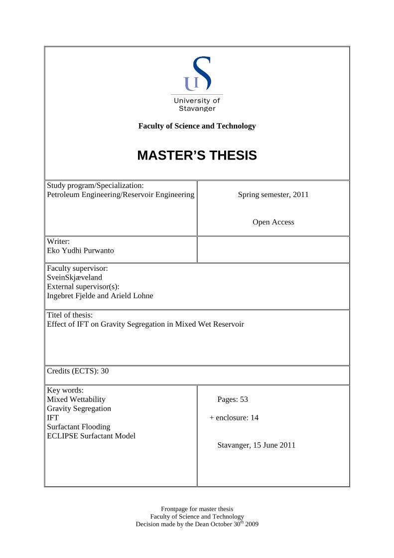
Wettability can be expressed conveniently by measuring the angle of contact at the liquid-
solid surface. This angle, which is normally measured through the water phase, is called
contact angle. As shown in Figure 2.1, a solid is water wet if the contact angle is less than
90o, and oil wet if it is more than 90o. Intermediate wet is identified when the contact angle is
close to 90o.
Apart from the contact angle measurement, several types of laboratory experiments for
determining wettability have been described in the literatures as reported by Anderson (1986).
One of the common methods is USBM (U.S. Bureau of Mines) which employs the wettability
index to express the wettability preferences of a core. In particular, a wettability index equals
to 0 indicates an intermediate wet, while value of +1 and -1 indicate strongly water wet and
strongly oil wet, respectively. Wettability index represents the average wettability of a core,
while the contact angle measures the wettability of a specific surface.
Figure 2.1 Determining wettability from contact angle (Raza et al., 1968).

6
2.1 Effect of Wettability on Relative Permeability
Rao et al. (1992) measured oil-water relative permeabilities from four rock-fluids systems
with different wettability preferences. The data obtained are presented in Figure 2.2. The
water wet characteristic of Beaverhill Lake (BL) rock-fluids is identified in which the end
point oil permeability is high (about 95% of the absolute permeability) and the end point
water permeability is low (about 10% of the absolute permeability). In contrast, the Crossfield
Cardium (CC) rock-fluids system clearly shows oil wet nature in which the end point water
permeability is much higher than the end point oil permeability.
The relative permeability curves for the Gilwood (GW) rock-fluids system indicate an
intermediate wet since the end point oil permeability is only about 30% of the absolute
permeability while the end point water permeability is almost 20% of the absolute. The
relative permeability curves for the Gilwood fluid – Berea (GB) system are comparable to
those of the intermediate wet GW system. However, the saturation band covered by water
permeability for the GB system is somewhat larger than that for the intermediate wet GW
system. Despite similar relative permeability characteristics, the authors found that the GB
system yielded significantly higher oil recoveries than in the intermediately wet GW system.
Therefore, the GB system is considered to be a mixed wet.
Figure 2.2 Oil-water relative permeability in various wettability preferences (Rao et al., 1992).

7
According to Raza et al. (1968), the end point water permeability is lower in the water wet
system when compared with the oil wet system because the residual oil in the water wet is
trapped as discontinuous droplets in the larger pores. These droplets block pore throats, thus
lowering the water permeability. On the other hand, the residual oil in the oil wet system is
located in the smaller pores and as film on the solid surfaces, where it has little effect on the
water flow.
2.2 Effect of Wettability on Capillary Pressure
Behbahani and Blunt (2004) performed an analysis of imbibition processes in mixed wet
rocks using pore scale modeling. Berea cores were saturated with Prudhoe Bay crude oil.
Then the samples were aged for between 0 and 240 hours to alter the wettability of the
samples from water wet towards mixed wettability. The capillary pressures from each sample
were measured and the results are shown in Figure 2.3. As the samples become more mixed
wet, the capillary pressure becomes lower and an increasing fraction of the curve lies below
zero, indicating oil wet properties. The capillary pressures above zero represent the process
when the samples imbibed water, while those below zero represent the process when the
samples imbibed oil. These results show that the mixed wet cores have the ability to imbibe
both water and oil.
Figure 2.3 Capillary pressure for different wettability states as represented by aging times, ta (Behbahani
and Blunt, 2004).

8
2.3 Effect of Wettability on Oil Recovery
Raza et al. (1968) described the process of waterflooding in water wet and oil wet system as
illustrated in Figure 2.4. Water displacing oil from a water wet pore is shown in Figure 2.4a.
The rock surface is preferentially wetted by the water, so water will move forward along the
pores wall, displacing oil in front of it. At some point, the remaining oil will become
disconnected, leaving an oil droplet trapped in the center of the pore. After the water front
passes, most of the remaining oil is immobile. Because of such immobility in this water wet
case, there is little or no oil production after water breakthrough.
Oil displacement process in an oil wet system is illustrated in Figure 2.4b. When the
waterflooding is started, the water will form continuous channels through the centers of the
larger pores, displacing oil in front of it. Oil is left in the smaller pores and as a continuous
film over the pore surfaces. Because much of the remaining oil is still continuous, additional
oil can be produced after water breakthrough. There is a tendency for the water to finger
through the larger pores and bypassing the oil in the smaller pores, thus earlier water
breakthrough is normally observed in an oil wet system. It is generally accepted that
waterflooding is less efficient in oil wet systems compared with water wet ones because of
earlier water breakthrough and more water must be injected to recover a given amount of oil.
Figure 2.4 Oil displacement process in (a) water wet and (b) oil wet system (Raza et al., 1968).

9
Salathiel (1973) compared waterflooding performance first in water wet core, and then in the
same core rendered mixed wettability. ROS (Remaining Oil Saturation) as a function of PV
(Pore Volume) injected is presented in Figure 2.5. As expected, there is very little or no oil
production after water breakthrough when the core is water wet. The final oil saturation is
about 35%. In the mixed wet core, more oil is recovered after the injection of the same
amount of water. The oil saturation keeps decreasing as long as the water is injected;
indicating small but finite oil permeability exists even at very low oil saturation. Very low
residual oil saturation (~10%) will be achieved by injection of many PV of water. The author
postulated that the very low residual oil saturation is obtained because of surface film
drainage mechanism.
Figure 2.5 Comparison of waterflooding behaviour in mixed-wet and water-wet cores (insert shows
extension of mixed wettability flooding data) (Salathiel, 1973).
Laboratory experiments done by Salathiel (1973) also demonstrated that the surface film
drainage of oil depends on the composition of the reservoir fluids and rock properties.
Therefore, the process does not occur in all mixed wet reservoirs. In those mixed wet
reservoirs where surface film drainage can occur, very low residual oil saturation can only be
achieved if depletion times are long enough for gravity segregation to be effective.
Wood et al. (1991) measured residual oil saturation in Endicott core sample, which possesses
typical mixed wettability characteristic. They showed that the remaining oil saturation is a
strong function of PV injected. After 1 PV injection, the ROS is 40%, whereas after 500 PV
the oil saturation is 22% and still falling. In addition, they also found that high vertical
permeability is essential for surface film drainage to be effective. These results reveal that
gravity segregation is an important oil recovery mechanism in mixed wet system.

10
3 SURFACTANT FLOODING
3.1 Introduction
Based on the process description, Green and Willhite (1998) divided oil recovery processes
into primary, secondary, and EOR process. Primary recovery is the recovery of oil by any of
the natural energy sources present in a reservoir without supplementary help from injected
fluids. These natural energy sources could be natural water drive, solution gas drive, gas cap
drive, fluid and rock expansion, or gravity drainage.
Secondary recovery uses additional energy from injection of water or gas to displace oil
toward producing wells (Lake, 1989). Water or gas is either injected into water or gas zone
for pressure maintenance or injected into oil zone to displace oil immiscibly according to
volumetric sweepout considerations. Waterflooding is perhaps the most common method of
secondary recovery.
Lake (1989) defined EOR as oil recovery by means of injection of materials not normally
present in reservoir. The injected fluids supplement the natural energy in the reservoir to
displace oil to a producing well. These processes differ from secondary recovery in such a
way that the injected fluids interact with the reservoir rock/oil system to create favorable
condition for oil recovery. These interactions include lower water-oil IFT, oil swelling, oil
viscosity reduction, wettability alteration, or favorable phase behavior.
Typically, a reservoir will undergo primary production followed by waterflooding (Green and
Willhite, 1998). Recovery by those processes might approach 35 to 50% IOIP when the
waterflooding reaches an economic limit. The remaining oil in the reservoir is a large and
attractive target for EOR methods. However, EOR is not necessarily applied in the last stage
of production. In some cases, EOR is applied as the initial stage of production. The usual
situation is viscous oil that would not be produced economically by primary mechanism or
waterflooding. In other cases, EOR might be applied after primary production (as a second
stage production).
Kate Van Dyke (1997) subdivided EOR techniques into three main categories; thermal
recovery, miscible injection, and chemical injection.
• Thermal recovery
This technique is intended to reduce the viscosity of heavy oil by applying heat, thus
improving the mobility and allowing the oil to be displaced to the producers. This is

11
the most common EOR technique. Hot water or steam drive, steam soak, and in situ
combustion are several methods for generating the heat.
• Miscible injection
Miscible injection is aimed to recover residual oil by using a displacing fluid which
mixes with oil in the reservoir. Typical miscible drive fluids include hydrocarbon
solvents, hydrocarbon gases, and carbon dioxide. Because those fluids are usually
more mobile than oil, they tend to bypass the oil resulting in low displacement
efficiency. This method is therefore best suited to high dip reservoirs.
• Chemical flooding
Chemical flooding involves the addition of one or more chemical compounds to the
injected water to improve displacement efficiency by either reducing water-oil IFT or
increasing the injected water viscosity, makes it less likely to bypass the oil.
Surfactant, polymer, and alkaline are among the chemicals used in chemical flooding.
3.2 Surfactants
Surfactant is a surface active agent that contains a hydrophobic (dislikes water) and a
hydrophilic (likes water) part as schematically illustrated in Figure 3.1, taken from Ottewill
(1984). The hydrophobic portion is often called the tail and the hydrophilic portion the head
of the molecule.
Figure 3.1 Schematic of surfactant molecule (Ottewill, 1984).
When surfactant is added into water-oil system at low concentration, the dissolved surfactant
molecules are dispersed as monomers and migrate to the interface between the oil and water
phase. As the surfactant concentration is increased, the surfactant molecules start to form

12
aggregates or micelles in a very narrow range of concentration called Critical Micelle
Concentration (CMC). Further increase of surfactant concentration results in the formation of
more micelles but relatively small change in monomer concentration. Figure 3.2 shows
water-oil system with surfactant concentration above CMC. The monomers reside at the
water-oil interface while the micelles are located either in the oil or water phase.
Figure 3.2 Water-oil system with surfactant concentration above CMC (Green and Willhite, 1998).
Water-oil IFT is a strong function of the surfactant’s monomers concentration. Figure 3.3
illustrates the general behavior of IFT as a function of surfactant concentration. The IFT
decreases significantly as surfactant concentration increases until the CMC is reached.
Surfactant added in excess of the CMC will not increase the concentration of monomers at the
water-oil interface, thus little change in water-oil IFT occurs.
Figure 3.3 IFT as a function of surfactant concentration (Green and Willhite, 1998).
Oil phase
Water phase
Micelle
Monomer
Micelle

13
3.3 Displacement Process
Craft and Hawkins (1991) defined the overall displacement efficiency (E) of any oil
displacement process as a product of volumetric (Ev) and microscopic displacement efficiency
(Ed). In the form of equation, it can be expressed as follow:
E = Ev × Ed (3.1)
The volumetric displacement efficiency refers to the effectiveness of the displacing fluid in
contacting the reservoir. It is governed by areal and vertical displacement efficiency. Both of
those efficiencies can be improved by maintaining favorable mobility ratio (M) throughout
the process.
M =
�kr µ� �D
�kr µ� �d
(3.2)
Where kr = relative permeability, µ = viscosity, subscript D and d = displacing and displaced
fluid, respectively. Favorable mobility ratio is achieved when the mobility of the displacing
fluid is lower than the mobility of the displaced fluid. In such situation, it is less likely for the
displacing fluid to bypass the displaced fluid. Polymer flooding is intended to decrease
mobility of the displacing fluid by increasing its viscosity.
The vertical displacement efficiency is affected by the density difference between the
displacing and displaced fluid. Large density difference can result in gravity segregation.
Gravity segregation at the displacement front is generally considered as a negative effect on
displacement efficiency. The effect is to bypass fluids at the top (under-riding) or bottom
(over-riding) of the reservoir, reducing the displacement efficiency in vertical cross section.
The vertical displacement efficiency is also affected by vertical permeability variation. In a
layered reservoir with vertical variation in permeability, the displacing fluid tends to flow in
14
the layer with the greatest permeability which leads to an uneven flow in different layers, thus
reducing vertical displacement efficiency.
The microscopic displacement efficiency refers to the effectiveness of the displacing fluid in
mobilizing the oil in the swept region. It is expressed in the magnitude of the residual oil
saturation (Sor) in the regions contacted by the displacing fluid. The microscopic displacement
efficiency can be improved by increasing the capillary number (Nc), a dimensionless ratio
between viscous and capillary forces. There are numerous alternatives to express the capillary
number. The following equations are some of the commonly used expressions.
Nc =
u × µIFT
=∆p × khL × IFT
(3.3)
Where u = velocity, µ = viscosity, ∆p = pressure drop, kh = horizontal permeability, L =
length, and IFT = interfacial tension between oil and water.
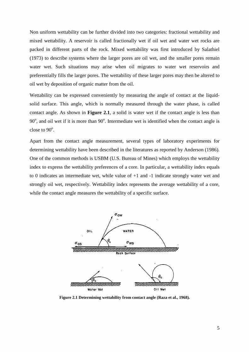
The relationship between the capillary number and residual oil saturation is commonly called
Capillary Desaturation Curve (CDC). Figure 3.4 shows typical CDCs in systems with
different pore size distribution. If the capillary number is increased beyond a particular value,
named critical capillary number, then the viscous forces will overcome the capillary forces
which are responsible for holding the oil in the porous media. Consequently, residual oil
saturation is decreased.
Figure 3.4 Capillary Desaturation Curve (Skjæveland and Kleppe, 1992).

15
The capillary number can be increased either by reducing the capillary forces or increasing
the viscous forces. Under actual reservoir conditions, the viscous forces cannot be increased
greatly because of the limitation on the injection pressure, which must not exceed the
fracturing pressure of the formation. As a result, fluid velocities within the reservoir are
generally limited to values of the order of 1 to 2 ft/day (Morrow, 1979).
The capillary forces, which are proportional to capillary pressure (Pc), are responsible for
holding fluids in porous media. As shown by Equation 3.4, it can be reduced by decreasing
IFT. Generally, IFT between water and oil can be in the range of 20 to 30 dynes/cm. By using
an appropriate surfactant system, this IFT can be reduced to 10-3 or 10-4 dynes/cm.
Pc =
2 × IFT × cos θr
(3.4)
Where IFT = interfacial tension between oil and water, θ = contact angle, and r = size of
capillary.
Figure 3.5, taken from Gilliland and Conley (1976), illustrates the typical process of a
surfactant flooding. Surfactant flooding is normally applied after waterflooding. Surfactant
solution is relatively expensive, so a limited volume (slug size) is usually used. The surfactant
slug therefore has to be displaced by water, usually containing polymer to reduce its mobility.
An oil bank will start to flow and mobilize any residual oil in front. Behind the oil bank, the
surfactant prevents the mobilized oil from being retrapped. If the surfactant concentration is
large enough, oil and water will be completely miscible hence no residual oil will be left in
the swept region. This is not a viable process, because it requires a large amount of surfactant.
If the surfactant is injected at low concentration, there may be up to three phase mixture (oil,
microemulsion, and water). In such condition, small amount of residual oil will still be
trapped in the swept region.
In some instances, polymer and alkaline can also be added into the surfactant slug to improve
the quality of the slug. Polymer is added to increase the slug viscosity, thus improving
volumetric displacement efficiency. Addition of alkaline into the surfactant slug could reduce
the required amount of the surfactant as the alkaline reacts with natural acids present in
certain crude oils to form surfactants within the reservoir. The surfactants formed in the
reservoir work in the same way as an injected surfactant.

16
Figure 3.5 Surfactant flooding process (Gilliland and Conley, 1976).
3.4 Important Factors in Surfactant Flooding
Surfactant solution, or usually called microemulsion, behavior is complex and dependent on a
number of parameters. Several parameters which are necessary to be considered in designing
and executing surfactant flooding project are presented in this section.
3.4.1 Salinity
Figure 3.6, taken from Healy et al. (1976), shows the effect of brine salinity on surfactant
solution (microemulsion) phase behavior. At low brine salinity, the surfactant is solubilized in
the water phase, creating a lower phase microemulsion. At high salinity, the surfactant is
driven out of the brine and solubilized in the oil phase. In this case, the microemulsion is an
upper phase microemulsion. At intermediate salinity, the system separates into three phases.
The microemulsion resides as a middle phase which is saturated with both oil and water. The
salinity at which the middle phase microemulsion contains an equal volume of oil and water is
defined as the optimal salinity for phase behavior (Healy et al., 1976).
Figure 3.6 Effect of salinity on microemulsion phase behavior (Healy et al., 1976).
17
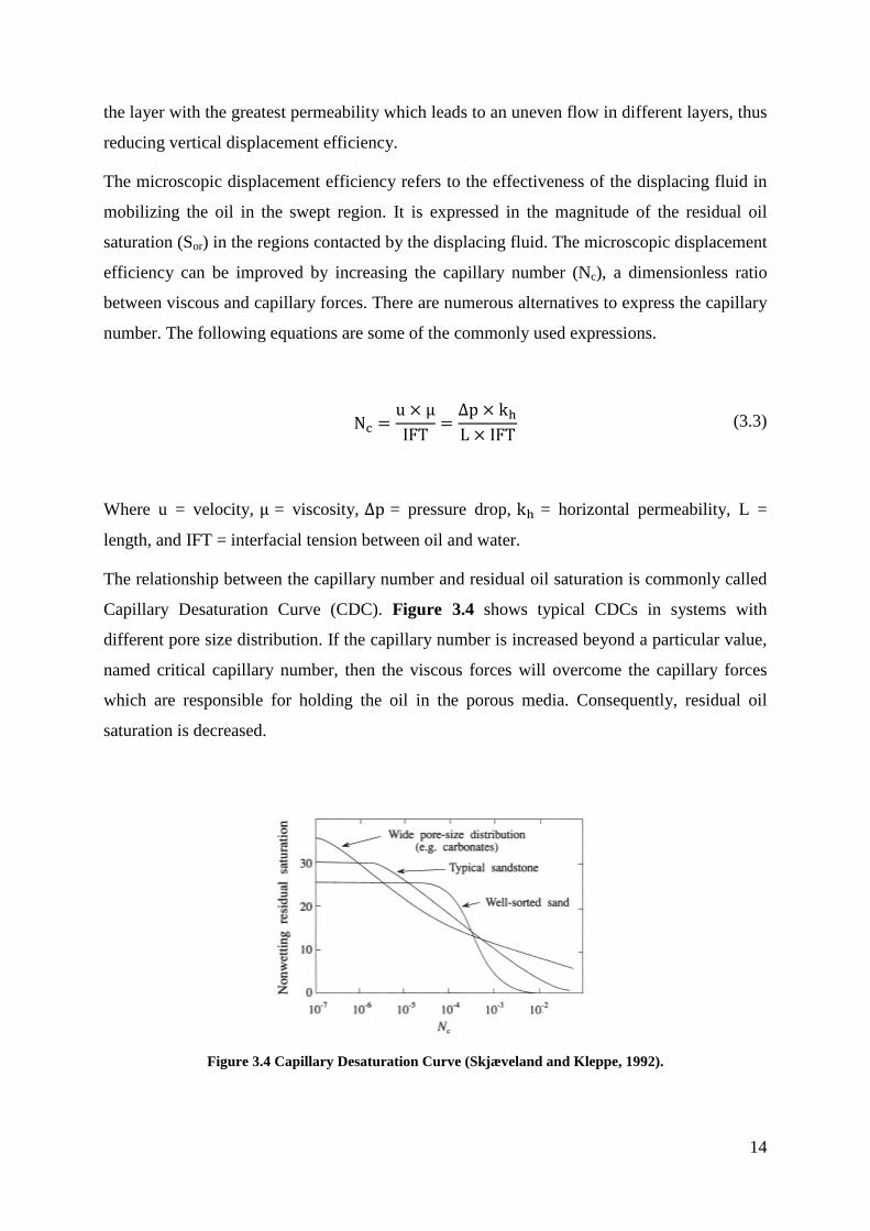
Figure 3.7, taken from Healy and Reed (1977), is a typical plot of IFT between equilibrium
phases and final oil saturation (Sof) as a function of salinity. σmo and σmw represent
microemulsion-oil IFT and microemulsion-water IFT, respectively. The value of salinity at
which σmo = σmw is called the optimal salinity for IFT (Healy et al., 1976). The authors
reported that the optimal salinity for IFT is usually very close to the optimal salinity for phase
behavior. The maximum oil recovery (minimum Sof) occurs at a salinity at or very near
optimal salinity. These results show that a surfactant flooding is most efficient when the IFT
between phases is low at both the leading and trailing edges of a surfactant slug. If the
microemulsion-oil IFT is too large, oil will not be displaced efficiently by the slug. On the
other hand, if the microemulsion-water IFT is too large, a relatively large residual saturation
of surfactant will be trapped at the trailing edge of the slug and the slug will be degraded as it
is transported through the rock.
Figure 3.7 IFT and final oil recovery as a function of salinity (Healy and Reed, 1977).
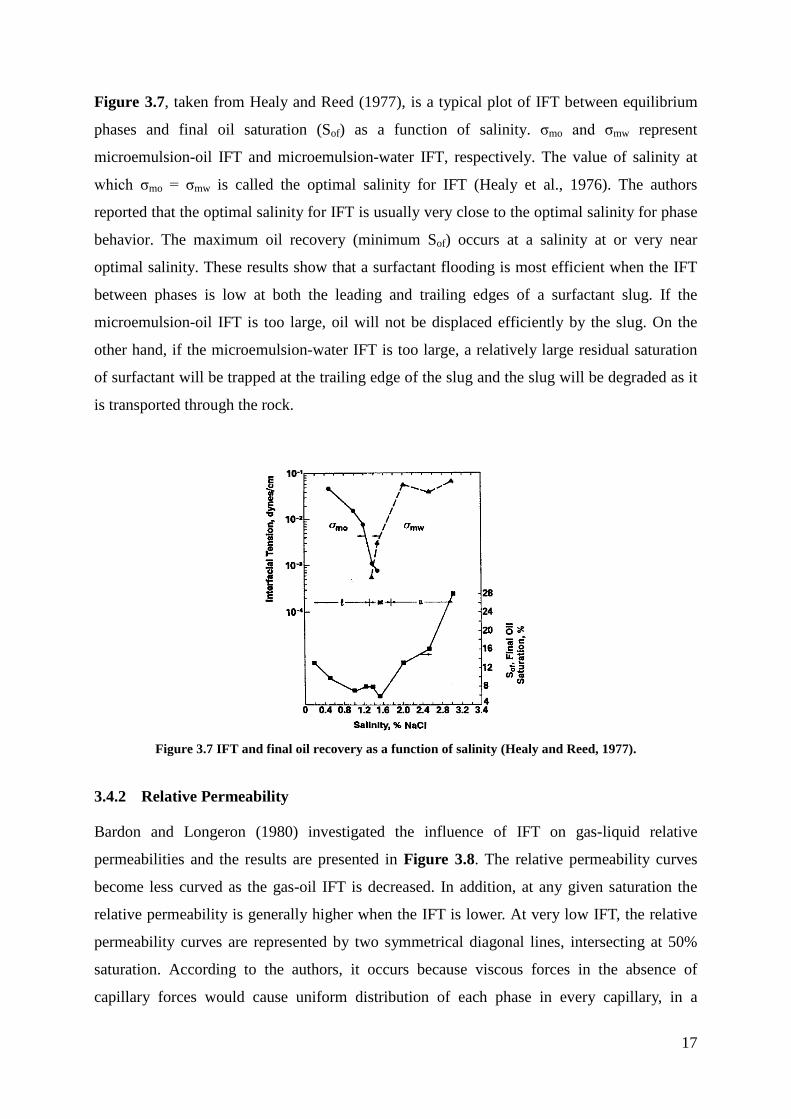
3.4.2 Relative Permeability
Bardon and Longeron (1980) investigated the influence of IFT on gas-liquid relative
permeabilities and the results are presented in Figure 3.8. The relative permeability curves
become less curved as the gas-oil IFT is decreased. In addition, at any given saturation the
relative permeability is generally higher when the IFT is lower. At very low IFT, the relative
permeability curves are represented by two symmetrical diagonal lines, intersecting at 50%
saturation. According to the authors, it occurs because viscous forces in the absence of
capillary forces would cause uniform distribution of each phase in every capillary, in a

18
proportion corresponding to its saturation. When the capillary forces are present, the viscous
forces would distribute the phases in the largest capillaries where the velocity is highest, while
in the smaller capillaries the distribution of the different phases is still determined by the
capillary forces.
Figure 3.8 Gas-oil relative permeability curves for various IFT values (Bardon and Longeron, 1978).
Similar results were presented by Batycky and McCaffery (1978). They conducted a series of
displacement processes for three water-oil IFT values which are nominally 50, 0.2, and 0.02
dynes/cm. They found that IFT reduction causes the relative permeability curves to become
less curved. A reduction in IFT also causes a reduction and the eventual removal of hysteresis
in the measured relative permeability curves. At IFT of 0.02 dynes/cm, the hysteresis
completely disappears, however the relative permeability curves are still slightly curved.
3.4.3 Wettability
Garnes et al. (1990) measured capillary desaturation curves measured on different North Sea
sandstone formations. The authors found that the North Sea Brent cores have lower critical
capillary number compared to Berea cores. Therefore, smaller change in capillary number
was required to mobilize the residual oil. They described that the more mixed wet behaviour
and the higher permeability of the North Sea Brent cores may account for this lower critical
capillary number.

19
Han Dong et al. (2006) conducted an experimental study to investigate waterflooding,
Alkaline/Surfactant/Polymer (ASP) flooding, and polymer flooding performance in different
wettability preferences. They found that displacement efficiency of waterflooding and ASP
flooding is greatly affected by the wettability of the core, but displacement efficiency of
polymer flooding is not sensitive to wettability. The oil recovery of waterflooding is optimum
at close to neutral wettability while water wet and oil wet conditions are favourable to obtain
high enhanced oil recovery for ASP flooding. Unfortunately, mixed wettability was not
included in their experiment.
3.4.4 Surfactant Loss
Green and Willhite (1998) reported that surfactant loss from an injected surfactant slug can
occur by at least three processes; precipitation, adsorption onto the porous medium, and phase
partitioning into a static or slow moving phase. These mechanisms result in retention of
surfactant in porous medium and deterioration of the surfactant composition, leading to poor
displacement efficiency.
The adsorption is strongly affected by the surfactant concentration. Figure 3.9, taken from
Skjæveland and Kleppe (1992), shows the typical adsorption isotherm for the adsorption of a
negatively charged surfactant onto positively charged adsorbent. As the surfactant
concentration increases, the adsorption increases until CMC is reached. Surfactant addition
above CMC will create micelles, but the amount of monomers is constant. According to the
authors, the micelles do not adsorb onto the solid, therefore surfactant adsorption is constant
above CMC.
Figure 3.9 Surfactant adsorption as a function of surfactant concentration (Skjæveland and Kleppe,
1992).
20
3.4.5 Gravity Segregation
Morrow (1979) presented an analysis to study the interplay of capillary, viscous, and
buoyancy forces in the mobilization of residual oil. The author found that the value of water-
oil IFT below which the oil droplet is mobilized, calculated by equating the hydrostatic
pressure difference with the capillary pressure difference, is equal to 10-3 dynes/cm. That is
the same order of magnitude as the IFT lowering needed to mobilize oil by viscous forces
when the flooding rates were restricted to field rates of about 1 ft/day. These results
demonstrate that the trapped oil mobilization could occur because of viscous or buoyancy
forces or some combination of both.
Morrow and Songkran (1982) investigate the correlation between Bond number (NB) and oil
recovery. Bond number is a dimensionless ratio between buoyancy and capillary forces, in the
form of equation it can be expressed as shown by Equation 3.5.
NB =
∆ρgR2
IFT (3.5)
Where ∆ρ = oil-water density difference, IFT = oil-water interfacial tension, g = gravitational
constant, R = characteristic length. Figure 3.10 shows plots of residual oil saturation as a
function of inverse Bond number at various capillary numbers. For the type of system under
their study, it was estimated that zero residual oil saturation will occur if the inverse Bond
number is less than about 3. When the inverse Bond number is greater than about 200, gravity
forces have no effect on the residual oil saturation, and the residual oil saturation depends
only on capillary number. These results demonstrate that the capillary pressure can also be
overcome by buoyancy forces.

21
Figure 3.10 Residual oil saturation as a function of inverse Bond number (Morrow and Songkran, 1982).
Hornof and Morrow (1987) observed front instabilities in displacement process at low water-
oil IFT, even the mobility ratio was at a favorable value. According to the authors, the
instabilities are caused by gravity segregation, which occurs if capillary and viscous forces are
insufficient to overcome the effect of buoyancy forces. These experiments reveal that the
degree of gravity segregation tends to increase with a decrease in IFT.
Schechter et al. (1991) investigated the effect of reduced IFT on gravity segregation in an
imbibition process. The authors found that a transition from capillary to gravity driven flow
occurred as the IFT was reduced. For low IFT and high permeability cores, buoyancy forces
might play a significant role in displacement mechanism. The authors also found that as the
inverse Bond number was decreased, an oil droplet that would have been trapped in the
capillary dominated flow could continue to flow if the gravitational forces became more
dominant.

22
4 METHODOLOGY AND MODEL SETUP
Nowadays, reservoir simulation is a very common practice in oil and service companies
which is used by most reservoir engineers. It is a very useful tool for estimating the future
behaviour of petroleum fields. In some cases, it can also be used for identifying particular
phenomena in a specific task.
All investigations in this study were performed by means of numerical simulation
experiments. Eclipse black oil model with surfactant option was used for simulating the
displacement process. In addition, Flow2D was also used for upscaling the relative
permeability curves. In the following sections, an overview about Eclipse and the
methodology carried out in this study are discussed.
4.1 Eclipse Overview
Eclipse is a reservoir simulator owned by SIS, a division of Schlumberger. It consists of two
separate simulators; Eclipse 100 for black oil modelling, and Eclipse 300 for compositional
modelling (Eclipse Technical Description, 2009). All simulations in this study were
conducted using the Eclipse 100. It is fully implicit, three phases, three dimensional, and
generally used for black oil modelling. The black oil model treats hydrocarbons as if they
have 2 components (oil and gas). Black oil model can be used whenever the hydrocarbon
compositions and properties do not vary significantly with pressure.
Eclipse 100 has the options to simulate several chemical species (polymer, surfactant,
alkaline, solvent, and foam). The surfactant option is the one that being employed in this
study. The important features of surfactant flooding can be modelled with this option. These
important features are discussed later in Section 4.1.1.
In this work, the input data for Eclipse simulation were prepared in free format using TextPad.
This text editor offers interesting features which improve user’s productivity when dealing
with a lot of data files. An Eclipse data input file is divided into the following sections;
1. RUNSPEC
This is the first section of an Eclipse data input file. It contains the run title, start
date, units, various problem dimensions (number blocks, wells, tables, etc.), flags
for phases present (oil, water, gas) and option switches (surfactant, polymer, etc.).

23
2. GRID
This section defines the basic geometry of the simulation grid and various rock
properties (porosity, absolute permeability).
3. PROPS
This section contains pressure and saturation dependent properties of the reservoir
fluids and rock. In surfactant model, properties of the surfactant must be provided
in this section as well. The saturation dependent properties include relative
permeability and capillary pressure data. The pressure dependent properties
include formation volume factor, density, and viscosity.
4. REGIONS
This section divides the computational grid into regions. In surfactant model, the
computational grid is divided into miscible and immiscible conditions. Different
sets of saturation functions corresponding to miscible and immiscible conditions
are assigned to the grid.
5. SOLUTION
This section defines the initial state (pressure, water-oil contact) of every grid
block in the reservoir.
6. SUMMARY
This section specifies a number of variables that are to be written to Summary files
after each time step of the simulation.
7. SCHEDULE
This section specifies the operations to be simulated (production and injection
controls, and constraints) and the times at which output reports are required.
Simulator tuning parameters may also be specified in this section.
4.1.1 Surfactant Model in Eclipse
The surfactant option can be activated by using SURFACT keyword under RUNSPEC
section. The surfactant is assumed to exist only in the water phase, so the amount of the
surfactant injected into the reservoir is specified as a concentration at a water injector by using
WSURFACT keyword under SCHEDULE section. The surfactant concentration will

24
determine the oil-water IFT based on a table provided by SURFST keyword under PROPS
section. The table supplies IFT as a function of surfactant concentration in the injected water.
The surfactant model does not provide detailed chemistry of a surfactant process, but it has
the capability to model the important features of a surfactant flooding on a full field basis
(Eclipse Technical Description, 2009). These important features include:
1. Reduction of capillary pressure.
Eclipse uses the value of IFT for calculating the capillary pressure. The capillary
pressure is given by the following equation.
Pcow = Pcow(Sw)
IFT(Csurf)IFT(Csurf = 0)
(4.1)
Where Pcow = oil-water capillary pressure, IFT(Csurf) and IFT(Csurf = 0) = oil-water
interfacial tension at the present and zero surfactant concentration, respectively. J
function is a dimensionless group that allows the capillary pressure to be correlated
with the rock properties. In many cases, all of the capillary pressure data from a
formation will be reduced to a single curve when the J function is plotted against the
saturation. If J function data are used, then an additional keyword (JFUNC) will be
required under GRID section to convert J function data into capillary pressure values
based on Equation 4.2.
Pc = J(Sw) × IFT × �
∅k�0.5
× Uconst (4.2)
Where Pc = capillary pressure, J(Sw) = dimensionless capillary pressure, Uconst = unit
conversion constant, ∅ and k = porosity and permeability, respectively.
2. Alteration of relative permeability curves from immiscible to miscible condition.
The capillary number is also calculated based on IFT. As the capillary number
increases, there will be a transition from immiscible to miscible condition. The user
has to provide a surfactant capillary desaturation function which describes the

25
transition from immiscible to miscible condition as a function of the capillary number.
It is done by implementing SURFCAPD keyword under PROPS section.
Relative permeability curves are modified based on the capillary number. The
modification is essentially a transition from immiscible relative permeability curves
(at low capillary number) to miscible relative permeability curves (at high capillary
number). Relative permeability curves for both miscible and immiscible condition
must be provided in PROPS section.
Figure 4.1 illustrates the calculation of the relative permeability curves for oil phase.
The end points of the curve are interpolated and both the immiscible and the miscible
curves are scaled to honour these points. The relative permeability values are looked
up on both curves, and the final relative permeability is taken as an interpolation
between these two values. The relative permeability for the water phase is calculated
in the same way as the oil case.
Figure 4.1 Calculation of the relative permeability (Eclipse Technical Description, 2009).
3. Alteration of the injected water viscosity due to surfactant addition.
The surfactant also changes the viscosity of the injected water. The surfactant
viscosity must be provided as a function of surfactant concentration using SURFVISC
keyword under PROPS section. Eclipse uses this input for calculating the water-
surfactant solution viscosity based on the following equation.

26
µws(Csurf, P) = µw(P)
µs(Csurf)µw(Pref)
(4.3)
Where µws = water-surfactant solution viscosity, µs = surfactant viscosity, and µw =
water viscosity.
4. Alteration of wettability.
This feature enables the modelling of wettability alteration of the rock due to the
accumulation of the surfactant. It can be activated by using SURFACTW keyword.
5. Surfactant adsorption onto the surface of reservoir rock.
In addition to the keywords mentioned above, the other optional keywords for
surfactant modelling in Eclipse include SURFADS and SURFROCK. Both of the
keywords are intended for describing the tendency of the surfactant to be adsorbed by
the reservoir rock.
4.2 Methodology
As described in the previous section, Eclipse surfactant model has the capability to model the
main features of a surfactant flooding process. These main features include:
1. Reduction in capillary pressure.
2. Alteration of relative permeability curves from immiscible to miscible condition.
3. Alteration of the injected water viscosity due to surfactant addition.
4. Alteration of rock wettability.
5. Surfactant adsorption onto the surface of reservoir rock.
This study was intended to investigate the effect of capillary pressure on gravity segregation.
To achieve this purpose, Eclipse black oil simulator was used and surfactant option was
activated to introduce the reduction in capillary pressure (by reducing IFT). In order to isolate
the mechanism of capillary pressure reduction from the other mechanisms, the Eclipse
surfactant model’s feature no.2 through no.5 need to be turned off.
27
The feature no.2 was turned off by using the same set of saturation functions both for miscible
and immiscible condition. The feature no.3 was excluded by specifying the same viscosity
both for water and water-surfactant solution. The features no.4 and 5 were neglected by
excluding any keywords related to these features.
Additionally, the surfactant solution was injected continuously. In such situation, the
reduction in IFT will follow the water front and be constant behind the water front. This will
allow us to conveniently assess the effect of any single parameter at a specific IFT without
worrying about the interference from IFT alteration during the displacement process.
4.3 Base Case Design
In this section, all input parameters used in base case model are presented. The input
parameters include model geometry, rock and fluids properties, saturation functions, wells
and simulation controls. The complete Eclipse input data for the base case can be found in
Appendix A.
4.3.1 Model Geometry and Rock Properties
A synthetic cross sectional two-dimensional (2D) model with one injection and one
production well was created to investigate the possible effects of gravity segregation on oil
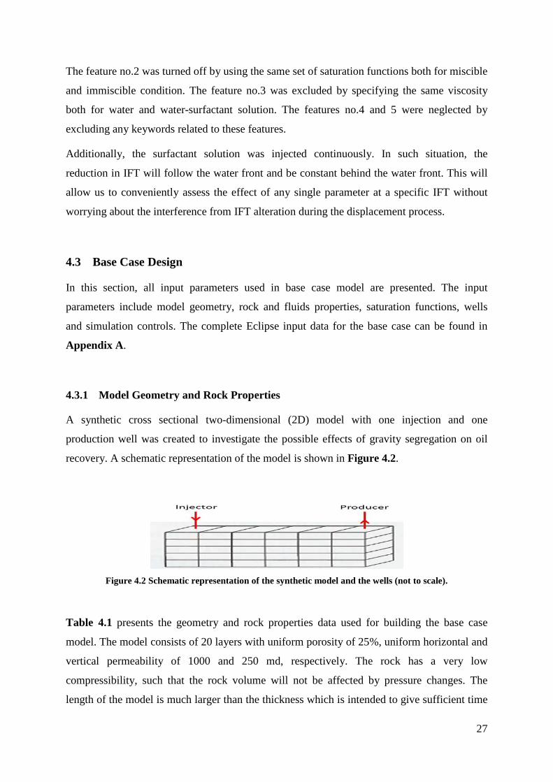
recovery. A schematic representation of the model is shown in Figure 4.2.
Figure 4.2 Schematic representation of the synthetic model and the wells (not to scale).
Table 4.1 presents the geometry and rock properties data used for building the base case
model. The model consists of 20 layers with uniform porosity of 25%, uniform horizontal and
vertical permeability of 1000 and 250 md, respectively. The rock has a very low
compressibility, such that the rock volume will not be affected by pressure changes. The
length of the model is much larger than the thickness which is intended to give sufficient time

28
for gravity forces to act on the system. This thin model may represent a single layer of a
reservoir.
Table 4.1 Geometry and rock properties data for base case.
Property Value
Length 500 m
Width 5 m
Height 2 m
Grid Dimension 100x1x20
Porosity 0.25
Horizontal permeability 1000 md
Vertical permeability 250 md
Rock Compressibility 1E-9 bar-1
4.3.2 Fluid Properties
Two phases (oil and water) were involved in the simulation. Table 4.2 summarizes the
properties of the fluids. Both the oil and water phase are assumed to be incompressible, such
that their Formation Volume Factors (FVF) were set at a value of 1 rm3/sm3 at all pressures.
Water and water-surfactant solution viscosity were set at the same value of 0.3 cp.
Table 4.2 Fluid properties.
Property Value
Bw 1 rm3/sm3 at all pressure
Bo 1 rm3/sm3 at all pressure
ρo 600 kg/m3 at STP
ρw 1000 kg/m3 at STP
µo 0.5 cp at all pressure
µw 0.3 cp at all pressure
µws 0.3 cp at all SC
4.3.3 Surfactant Properties
Table 4.3 summarizes the IFT as a function of surfactant concentration. Plot of the data is
presented in Figure 4.3. As can be seen, surfactant concentration of 6 kg/m3 is considered as
the CMC of the surfactant system, in which further surfactant addition above this value will
not change the IFT.

29
Table 4.3 IFT as a function of surfactant concentration.
Surf Conc, kg/m3 IFT, dynes/cm
0 25
0.5 1
1.5 0.1
3 0.01
6 0.001
10 0.001
Figure 4.3 IFT as a function of surfactant concentration.
Table 4.4 gives the surfactant capillary desaturation data. In Eclipse, the water-oil miscibility
is expressed by a number between 0 and 1. A value of 0 implies immiscible condition and a
value of 1 represents miscible condition. It is worth to emphasize that the surfactant capillary
desaturation data will not affect the results in this study since the same saturation functions
apply for both immiscible and miscible condition.
Table 4.4 Surfactant capillary desaturation data.
Log Nc Miscibility
-9.00 0.00
-4.50 0.00
-2.00 1.00
10.00 1.00
1.E-04
1.E-03
1.E-02
1.E-01
1.E+00
1.E+01
1.E+02
0 2 4 6 8 10
IFT,
dyn
es/c
m
Surfactant Concentration, kg/m3
CMC

30
4.3.4 Saturation Functions
The relative permeability and capillary pressure data were taken from a mixed wet core from
a North Sea reservoir. Figure 4.4 shows the plot of relative permeability as a function of
water saturation in linear and logarithmic scale whereas the plot of the imbibition
dimensionless capillary pressure (J function) as a function of water saturation is presented in
Figure 4.5. These data were used for both miscible and immiscible conditions.
Figure 4.4 Mixed wet relative permeability in linear (left) and logarithmic scale (right).
Figure 4.5 Mixed wet dimensionless imbibition capillary number.
As can be seen in Figure 4.4, the relative permeability curves for both of the oil and water
phase have high curvature, low residual saturation, and long tail at low saturation.
Additionally, the end point water and oil relative permeability are comparable (0.85% and
0.93% of absolute permeability, respectively). Figure 4.5 shows that the capillary pressure
becomes negative as the water phase saturation increases. Those are the typical characteristics
of a mixed wet system.
31
4.3.5 Wells and Simulation Controls
Boundary conditions were set using two wells, placed in the first and the last block (see
Figure 4.2) with well connection factors corresponding to open end faces. Open end faces
were implemented to exclude the additional pressure drop due to the wells, so the simulation
would resemble displacement process in a particular part of a reservoir. It was done by
calculating the Well Connection Factor (WCF) with the following equation and using it as an
input parameter under COMPDAT keyword.
WCF =
khA
�∆x2� (4.4)
Where kh = horizontal permeability, A = cross sectional area, and ∆x = grid block size in x
direction. Both of the wells were perforated in all layers. The production well was controlled
by minimum bottomhole pressure of 200 bars, while the injection well was controlled by the
injection velocity of 0.5 m/day. However, Eclipse does not provide injection velocity as a well
controlling parameter. Therefore, the injection fluid velocities were converted into injection
rates, and then included in the Eclipse input data by using RESV keyword.

32
5 RESULTS AND DISCUSSION
5.1 Simulation Model Validation
As a starting point, the simulation model is validated by evaluating the effect of IFT on oil
recovery in a mixed wet one-dimensional (1D) horizontal model. Two IFT values were used
(25 and 1 dynes/cm) and both of the cases were run at the same injection velocity of 0.5
m/day. The production profiles for both of the cases are presented in Figure 5.1. There are at
least two observations that can be made from these results. First, most of the oil production
occurs before water breakthrough. However, considerable amount of oil production is also
observed after the water breakthrough. The recovery factor at 5 PV injected is about 73% and
keeps increasing if the water injection continues. The continuously increasing oil production
after water breakthrough occurs because the oil wet surfaces in the larger pores of the mixed
wet system help maintaining the continuity of oil phase at low oil saturation. These results
possess a similar trend as the characteristic of mixed wet reservoir as reported by Salathiel
(1973).
The second observation is that both of the cases give the same production profiles. It is
expected since the same saturation functions are used for both immiscible condition (at high
IFT) and miscible condition (at low IFT). Additionally, it is expected that there was no
vertical gravity segregation acting in the one-dimensional system because the fluids were
allowed to move in horizontal direction only. These results suggest that gravity segregation is
the only mechanism that will be affected by changing IFT in this simulation model. Isolating
gravity segregation from other mechanisms is very important, since this study focuses on
investigating the mechanism of gravity segregation.
5.2 Effect of Gravity Segregation on Oil Recovery
Two runs were created using the two-dimensional base case model with high (25 dynes/cm)
and low (1 dynes/cm) IFT. Both of the cases were run at the same velocity of 0.5 m/day.
Figure 5.2 shows the production profiles from both of the cases, along with the result from
the one-dimensional model. It can be seen that the final oil recoveries from both of the two-
dimensional models are higher than that given by the one-dimensional model. The highest oil
recovery is given by the two-dimensional model with low IFT, 78% of IOIP, while the two-
dimensional model with high IFT has produced almost 73%, and the one-dimensional model
has recovered 69% of IOIP after 5 PV injected.

33
Figure 5.1 Production profiles from 1D model with IFT of 1 and 25 dynes/cm. The curve for IFT of 25
dynes/cm is not seen due to overlap with the other curve.
Figure 5.2 Production profiles from 1D and 2D model with IFT of 25 and 1 dyne/cm.
The oil recovery mechanisms in those three cases would be better understood by investigating
their oil saturation distributions. Figure 5.3 visualizes the oil saturation distribution after 5 PV
injections for all of the three cases. In the case of one-dimensional model, no gravity
segregation is observed because the fluids moved in horizontal direction only (see Figure
5.3a). The oil saturation is lower at the inlet (the injection well) and increases toward the
outlet (the production well). The oil phase was displaced solely by horizontal viscous forces
toward the production well.
Water breakthrough

34
In both of the two-dimensional models, vertical gravity segregations are observed. Gravity
forces cause the less dense phase (oil) to move upward and the denser phase (water) to move
downward. This condition results in an upward increasing trend in oil saturation. More even
distribution of oil saturation is observed in the model with high IFT (see Figure 5.3b) when
compared with the model with low IFT (Figure 5.3c). In the model with low IFT, most of the
oil phase has travelled to the top of the model creating a very thin layer with high oil
saturation. These results clearly demonstrate that gravity segregation acting behind the
displacement front may increase the oil recovery by accumulating the oil phase at the top of
the model, thus improving the effective horizontal oil mobility. Capillary forces will act
against this segregation. A reduction in IFT will decrease the capillary forces, thus increasing
the magnitude of gravity segregation. Further investigations on the effect of IFT on gravity
segregation are discussed later in Section 5.4.
Figure 5.3 Oil saturation distributions in (a) 1D model, and 2D models with IFT of (b) 25 dynes/cm and (c)
1 dynes/cm.
35
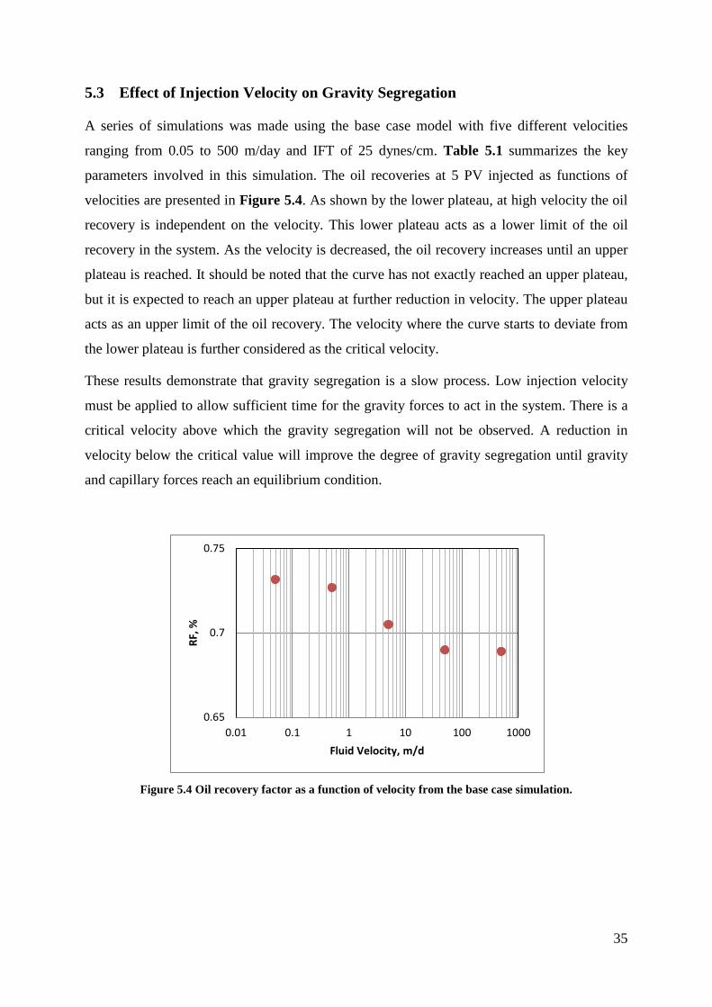
5.3 Effect of Injection Velocity on Gravity Segregation
A series of simulations was made using the base case model with five different velocities
ranging from 0.05 to 500 m/day and IFT of 25 dynes/cm. Table 5.1 summarizes the key
parameters involved in this simulation. The oil recoveries at 5 PV injected as functions of
velocities are presented in Figure 5.4. As shown by the lower plateau, at high velocity the oil
recovery is independent on the velocity. This lower plateau acts as a lower limit of the oil
recovery in the system. As the velocity is decreased, the oil recovery increases until an upper
plateau is reached. It should be noted that the curve has not exactly reached an upper plateau,
but it is expected to reach an upper plateau at further reduction in velocity. The upper plateau
acts as an upper limit of the oil recovery. The velocity where the curve starts to deviate from
the lower plateau is further considered as the critical velocity.
These results demonstrate that gravity segregation is a slow process. Low injection velocity
must be applied to allow sufficient time for the gravity forces to act in the system. There is a
critical velocity above which the gravity segregation will not be observed. A reduction in
velocity below the critical value will improve the degree of gravity segregation until gravity
and capillary forces reach an equilibrium condition.
Figure 5.4 Oil recovery factor as a function of velocity from the base case simulation.
0.65
0.7
0.75
0.01 0.1 1 10 100 1000
RF, %
Fluid Velocity, m/d
36
Table 5.1 Key parameters in the base case model.
Key Parameters Value IFT 25 dynes/cm Vertical permeability 250 md Horizontal permeability 1000 md Oil density 600 kg/m3 Model thickness 2 m
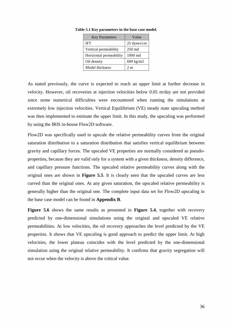
As stated previously, the curve is expected to reach an upper limit at further decrease in
velocity. However, oil recoveries at injection velocities below 0.05 m/day are not provided
since some numerical difficulties were encountered when running the simulations at
extremely low injection velocities. Vertical Equilibrium (VE) steady state upscaling method
was then implemented to estimate the upper limit. In this study, the upscaling was performed
by using the IRIS in-house Flow2D software.
Flow2D was specifically used to upscale the relative permeability curves from the original
saturation distribution to a saturation distribution that satisfies vertical equilibrium between
gravity and capillary forces. The upscaled VE properties are normally considered as pseudo-
properties, because they are valid only for a system with a given thickness, density difference,
and capillary pressure functions. The upscaled relative permeability curves along with the
original ones are shown in Figure 5.5. It is clearly seen that the upscaled curves are less
curved than the original ones. At any given saturation, the upscaled relative permeability is
generally higher than the original one. The complete input data set for Flow2D upscaling in
the base case model can be found in Appendix B.
Figure 5.6 shows the same results as presented in Figure 5.4, together with recovery
predicted by one-dimensional simulations using the original and upscaled VE relative
permeabilities. At low velocities, the oil recovery approaches the level predicted by the VE
properties. It shows that VE upscaling is good approach to predict the upper limit. At high
velocities, the lower plateau coincides with the level predicted by the one-dimensional
simulation using the original relative permeability. It confirms that gravity segregation will
not occur when the velocity is above the critical value.
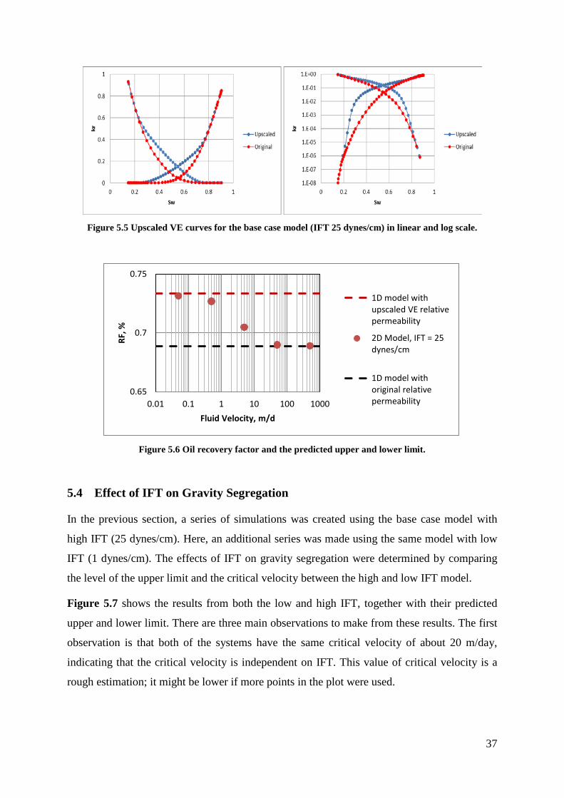
37
Figure 5.5 Upscaled VE curves for the base case model (IFT 25 dynes/cm) in linear and log scale.
Figure 5.6 Oil recovery factor and the predicted upper and lower limit.
5.4 Effect of IFT on Gravity Segregation
In the previous section, a series of simulations was created using the base case model with
high IFT (25 dynes/cm). Here, an additional series was made using the same model with low
IFT (1 dynes/cm). The effects of IFT on gravity segregation were determined by comparing
the level of the upper limit and the critical velocity between the high and low IFT model.
Figure 5.7 shows the results from both the low and high IFT, together with their predicted
upper and lower limit. There are three main observations to make from these results. The first
observation is that both of the systems have the same critical velocity of about 20 m/day,
indicating that the critical velocity is independent on IFT. This value of critical velocity is a
rough estimation; it might be lower if more points in the plot were used.
0.65
0.7
0.75
0.01 0.1 1 10 100 1000
RF, %
Fluid Velocity, m/d
1D model withupscaled VE relativepermeability
2D Model, IFT = 25dynes/cm
1D model withoriginal relativepermeability

38
The second observation is that the effect of IFT reduction becomes more significant as the
injection velocity is decreased. The third observation is that the upper limit significantly
improves, from 73% to 85%, when the IFT is reduced from 25 to 1 dynes/cm. It indicates that
capillary forces restrict the gravity segregation, thus reducing the capillary pressure (by
reducing IFT) will increase the degree of gravity segregation.
The upper limit improvement was then calculated by using Equation 5.1. It was found that
the upper limit increases by 16% when the IFT is reduced from 25 to 1 dynes/cm. Only a
moderate reduction in IFT down to 1 dynes/cm (compared to standard surfactant flooding)
was used in these simulations. These results show that there is a considerable potential
increase in oil recovery given by gravity segregation mechanism. All the main observations
from this base case simulation are summarized in Table 5.2.
% Upper Limit Improvement = �(Upper Limit )High IFT − (Upper Limit)Low IFT
(Upper Limit)High IFT� (5.1)
Figure 5.7 Oil recovery factor and the predicted upper and lower limit (kv = 250 md, kh = 1000 md, ρo =
600 kg/m3, H = 2 m).
Table 5.2 Main observations from the base case simulation.
Observation Result Critical Velocity, m/day ̴ 20 Upper Limit (IFT = 25 dynes/cm), % 73 Upper Limit (IFT = 1 dynes/cm), % 85 Upper Limit Improvement, % 16
0.65
0.7
0.75
0.8
0.85
0.9
0.01 0.1 1 10 100 1000
RF, %
Fluid Velocity, m/d
1D, VE upscaled, IFT =25 dynes/cm
1D, VE Upscaled, IFT =1 dynes/cm
2D, IFT = 1 dynes/cm
2D, IFT = 25 dynes/cm
1D, original relativepermeability

39
The VE upscaled relative permeability curves for both the high and low IFT are presented in
Figure 5.8. It can be seen that the low IFT’s upscaled curves are represented by straight lines,
whereas the high IFT’s upscaled curves have somewhat strong curvature. This indicates that
the capillary forces in the low IFT system are almost completely eliminated, as shown by the
straight lines of the relative permeability curves. Therefore, the upper limit of the low IFT
model is significantly higher than that given by the high IFT model.
Figure 5.8 Upscaled VE relative permeability curves for the base case model with IFT of 25 and 1
dynes/cm.
5.5 Effect of IFT on Gravity Segregation in Various Conditions
The key parameters presented in Table 5.1 are expected to affect the behaviour of gravity
segregation. In this section, the effects of each of those parameters were investigated to study
in what way they affect the segregation process. The investigations were performed by
varying one parameter while the other parameters were kept unchanged. The simulation cases
are summarized in Table 5.3. The highlighted parameter is the one being investigated in each
case.
Table 5.3 Simulation cases.
Case Number kv, md kh, md ρo, kg/m3 H, m Base Case 250 1000 600 2 Case 1 1000 1000 600 2 Case 2 250 250 600 2 Case 3 250 1000 850 2 Case 4 250 1000 600 20
0
0.2
0.4
0.6
0.8
1
0 0.5 1
kr
Sw
Upscaled, IFT = 25dynes/cm
Upscaled, IFT = 1dynes/cm

40
In each case, two series of simulations at various injection velocities were created. One series
is for the model with high IFT (25 dynes/cm) and the other series is for the model with low
IFT (1 dynes/cm). The corresponding upper and lower limits for the low and high IFT model
were also created by one-dimensional simulations with original and upscaled VE relative
permeability curves. The simulation results from each case were then compared with the
results given by the base case model as shown in Table 5.2.
5.5.1 Case 1: Effect of Vertical Permeability
The simulation results from case 1 are presented in Figure 5.9. In this case, the vertical
permeability is four times higher than that in the base case. The main observations from this
case are summarized in Table 5.4. For comparison, the observations from the base case
simulations are also presented in the same table.
Figure 5.9 Simulation results from the case 1.
Table 5.4 Observations from the case 1 and the base case
Observations Case 1, kv = 1000 md Base Case, kv = 250 md
Critical Velocity, m/day ̴ 80 ̴ 20 Upper Limit (IFT = 25 dynes/cm), % 73 73 Upper Limit (IFT = 1 dynes/cm), % 85 85 Upper Limit Improvement, % 16 16
The critical velocity for both the low and high IFT is estimated to be 80 m/day, which is four
times higher than that given by the base case (20 m/day). These results demonstrate that
0.65
0.7
0.75
0.8
0.85
0.9
0.01 0.1 1 10 100 1000
RF, %
Fluid Velocity, m/d
Upper Limit, 25dynes/cm
Upper Limit, 1dynes/cm
IFT = 1 dynes/cm
IFT = 25 dynes/cm
Lower Limit

41
increasing the vertical permeability by a given factor will increase the critical velocity by the
same factor.
Obviously, the lower limit is not affected by the vertical permeability. So are the upper limits
for both the high and low IFT model. Flow2D calculates the J-scaling based on the following
equation.
Pc = J × IFT × �
∅kx
(5.2)
Where Pc = capillary pressure, J = dimensionless capillary pressure, ∅ = porosity, and kx =
horizontal permeability in x direction. The equation shows that vertical permeability is not
accounted for calculating the J-scaling of capillary pressure in the Flow2D software.
Therefore, changing vertical permeability will not affect the upper and lower limit. However,
at any given velocity between the upper and lower plateau, reducing IFT in the system with
higher vertical permeability may give higher oil recovery improvement. For example, at
velocity of 5 m/day, the case 1 gives almost 5% improvement of oil recovery by reducing the
water-oil IFT from 25 to 1 dynes/cm, while the same reduction of IFT in the base case gives
only about 2% improvement.
5.5.2 Case 2: Effect of Horizontal Permeability
The simulation results from case 2 are presented in Figure 5.10. In this case, the horizontal
permeability is four times lower than that in the base case. The main observations from this
case are summarized in Table 5.5. For comparison, the observations from the base case
simulations are also presented in the same table.
Comparing the results from the case 2 and the base case, it can be observed that the horizontal
permeability has no influence in the critical velocity. In both of the cases, gravity segregation
occurs at the same velocity of about 20 m/day. It occurs simply because the horizontal
permeability does not affect the vertical segregation rate.
The upper limit increases from 71 to 84 dynes/cm when the IFT is reduced from 25 to 1
dynes/cm. Both of those upper limits are slightly lower than those given by the base case

42
simulations. It occurs because the capillary pressure is inversely proportional to square root of
horizontal permeability (see Equation 5.1). As the horizontal permeability is decreased, the
capillary pressure will increase, thus less oil will be recovered. However, the upper limit
improvement is higher for the case 2. It indicates that lowering IFT will give more significant
effect if the capillary pressure of the system is originally high.
Figure 5.10 Simulation results from the case 2.
Table 5.5 Observations from the case 2 and the base case.
Results Case 2, kh = 250 md Base Case, kh = 1000 md Critical Velocity, m/day ̴ 20 ̴ 20 Upper Limit (IFT = 25 dynes/cm), % 71 73 Upper Limit (IFT = 1 dynes/cm), % 84 85 Upper Limit Improvement, % 18 16
5.5.3 Case 3: Effect of Oil Density
The simulation results from case 3 are presented in Figure 5.11. In this case, the oil density
was varied while the water density was kept the same as the base case. The density difference
is 150 kg/m3, which is 37.5% of the density difference in the base case. The main
observations from this case are summarized in Table 5.6. For comparison, the observations
from the base case simulations are also presented in the same table.
The critical velocity is estimated to be 8 m/day or lower, which is approximately 40% of the
critical velocity given by the base case. This change is at the same order of magnitude as the
0.65
0.7
0.75
0.8
0.85
0.9
0.01 0.1 1 10 100 1000
RF, %
Fluid Velocity, m/d
Upper Limit, 25dynes/cm
Upper Limit, 1dynes/cm
IFT = 1 dynes/cm
IFT = 25 dynes/cm
Lower Limit

43
change of the density difference (37.5%). These results demonstrate that the critical velocity
will decrease by a given factor when the density difference is decreased by the same factor.
The upper limits for high and low IFT are 70 and 83%, respectively. Both of those limits are
slightly lower than those given by the base case. It occurs because density difference is the
driving force in gravity segregation. As the driving force is decreased, the magnitude of
gravity segregation will also decrease, thus less oil will be recovered. However, the upper
limit improvement is higher for the case 3. It demonstrates that lowering IFT will give more
significant effect when the driving force of gravity segregation is originally low.
Despite the oil density was varied from very low (600 kg/m3) to very high density (850
kg/m3), the effect on segregation is small. It indicates that the magnitude of gravity
segregation is relatively insensitive to the magnitude of the density difference for the range of
densities normally encountered in actual oil production operations.
It is worth to mention that the oil viscosities were kept constant at 0.5 cp for those runs,
although physically, a change in oil density should be accompanied by a change in viscosity.
The reason for not changing the oil viscosity when the density was changed was simply
because the objective of these simulations was to isolate the influence of the density
difference on gravity segregation.
Figure 5.11 Simulation results from the case 3.
0.65
0.7
0.75
0.8
0.85
0.9
0.01 0.1 1 10 100 1000
RF, %
Fluid Velocity, m/d
Upper Limit, 25dynes/cm
Upper Limit, 1dynes/cm
IFT = 1 dynes/cm
IFT = 25 dynes/cm
Lower Limit

44
Table 5.6 Observations from the case 3 and the base case.
Results Case 3, ρo = 850 kg/m3 Base Case, ρo = 600 md
Critical Velocity, m/day ̴ 8 ̴ 20 VE Limit (IFT = 25 dynes/cm), % 70 73 VE Limit (IFT = 1 dynes/cm), % 83 85 VE Limit Improvement, % 18.5 16
5.5.4 Case 4: Effect of Model Thickness
In the case 4, the model thickness is ten times larger than that in the base case. The simulation
results are presented in Figure 5.12. The main observations from this figure, along with the
observations from the base case, are summarized in Table 5.7.
The critical velocity is estimated to be 5 m/day, which is ten times lower than that given by
the base case. These results clearly demonstrate that an increase in the model thickness by a
given factor will decrease the critical velocity by the same factor. It occurs because the oil
phase has to travel in a longer vertical distance in order to reach the top of the model.
The upper limit increases from 83% to 87% when the water-oil IFT is decreased from 25 to 1
dynes/cm. Both of those upper limits are higher than those given by the base case simulations.
It occurs because the hydrostatic pressure of the water phase is higher in the thicker model.
Therefore, the water phase has higher potential to move downwards and displace the oil phase
to the top of the model. When the potential of having gravity segregation is already high,
lowering IFT will only give small oil recovery improvement. It is shown by the upper limit
which increases only by 5% when the IFT is decreased from 25 to 1 dynes/cm. It is much less
than the upper limit improvement given by the base case (thin model), 16%.
Table 5.7 Observations from the case 4 and the base case
Results Case 4, H = 20 m Base Case, H = 2 m Critical Velocity, m/day ̴ 5 ̴ 50 VE Limit (IFT = 25 dynes/cm), % 83 73 VE Limit (IFT = 1 dynes/cm), % 87 85 VE Limit Improvement, % 5 16

45
Figure 5.12 Simulation results from the case 4.
5.5.5 A Correlation for Predicting the Critical Velocity
Critical velocity represents a condition when the gravity forces start to overcome the viscous
forces, thus gravity segregation occurs. The gravity forces are driven by the density
difference, while pressure gradient is the driving mechanism in the viscous forces. A
correlation between the critical velocity and these two parameters (density difference and
pressure gradient) was established. The correlation is based upon the simulation results
previously discussed. Vertical permeability and thickness would also be taken into account in
the correlation since they affect the critical velocity (see Section 5.5.1 and Section 5.5.4).
An attempt was made to correlate the oil recoveries with viscous-gravity forces ratio (Rvg) in
the form of the following equation.
Rvg =
∆pL
× kh∆ρ × g × kv
�hL� (5.2)
Where Δp/L = pressure gradient, Δρ = density difference, g = gravitational acceleration, kv =
vertical permeability, kh = horizontal permeability, h = thickness, and L = length. This
dimensionless number was chosen since it contains all the pertinent parameters. It should be
noted that Equation 5.2 is slightly different from the viscous-gravity forces ratio proposed by
Stalkup (1983) in which h is the denominator and L is the numerator. Stalkup’s equation is
applicable for evaluating gravity segregation at the displacement front, whereas this study
0.65
0.7
0.75
0.8
0.85
0.9
0.01 0.1 1 10 100 1000
RF, %
Fluid Velocity, m/d
Upper Limit, 25dynes/cm
Upper Limit, 1dynes/cm
IFT = 1 dynes/cm
IFT = 25 dynes/cm
Lower Limit

46
focuses on gravity segregation that takes place behind the displacement front. The required Δp
data from all of the simulations carried out in this study are presented in Appendix C.
Figure 5.13 through Figure 5.16 show oil recovery factor as a function of Rvg for all of the
cases. It can be seen that in each case, the curves start to deviate from the lower plateau when
Rvg is approximately one. It indicates that the gravity segregation will occur when the gravity
forces are higher than the viscous forces.
These results demonstrate that viscous-gravity forces ratio can be used as an indicator to
determine under which condition gravity segregation occurs. For a system with a given water-
oil density difference, horizontal and vertical permeability, and geometry (length and height),
one can use this correlation to predict the required pressure difference or velocity for gravity
segregation to occur.
Figure 5.13 Oil recovery factor as a function of Rvg for the base case.
Figure 5.14 Oil recovery factor as a function of Rvg for the case 1.
0.65
0.7
0.75
0.8
0.85
0.9
0.001 0.01 0.1 1 10 100
RF, %
Rvg
IFT = 1 dynes/cm
IFT = 25 dynes/cm
0.65
0.7
0.75
0.8
0.85
0.9
0.001 0.01 0.1 1 10 100
RF, %
Rvg
IFT = 1 dynes/cm
IFT = 25 dynes/cm
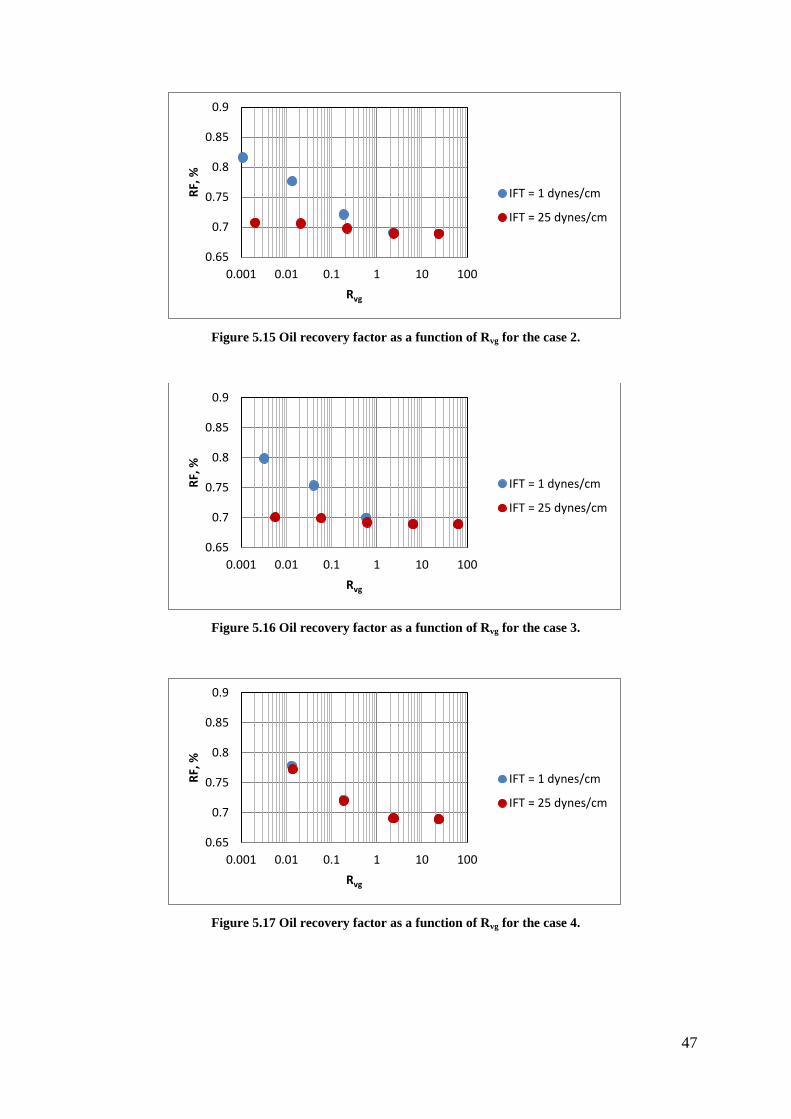
47
Figure 5.15 Oil recovery factor as a function of Rvg for the case 2.
Figure 5.16 Oil recovery factor as a function of Rvg for the case 3.
Figure 5.17 Oil recovery factor as a function of Rvg for the case 4.
0.65
0.7
0.75
0.8
0.85
0.9
0.001 0.01 0.1 1 10 100
RF, %
Rvg
IFT = 1 dynes/cm
IFT = 25 dynes/cm
0.65
0.7
0.75
0.8
0.85
0.9
0.001 0.01 0.1 1 10 100
RF, %
Rvg
IFT = 1 dynes/cm
IFT = 25 dynes/cm
0.65
0.7
0.75
0.8
0.85
0.9
0.001 0.01 0.1 1 10 100
RF, %
Rvg
IFT = 1 dynes/cm
IFT = 25 dynes/cm
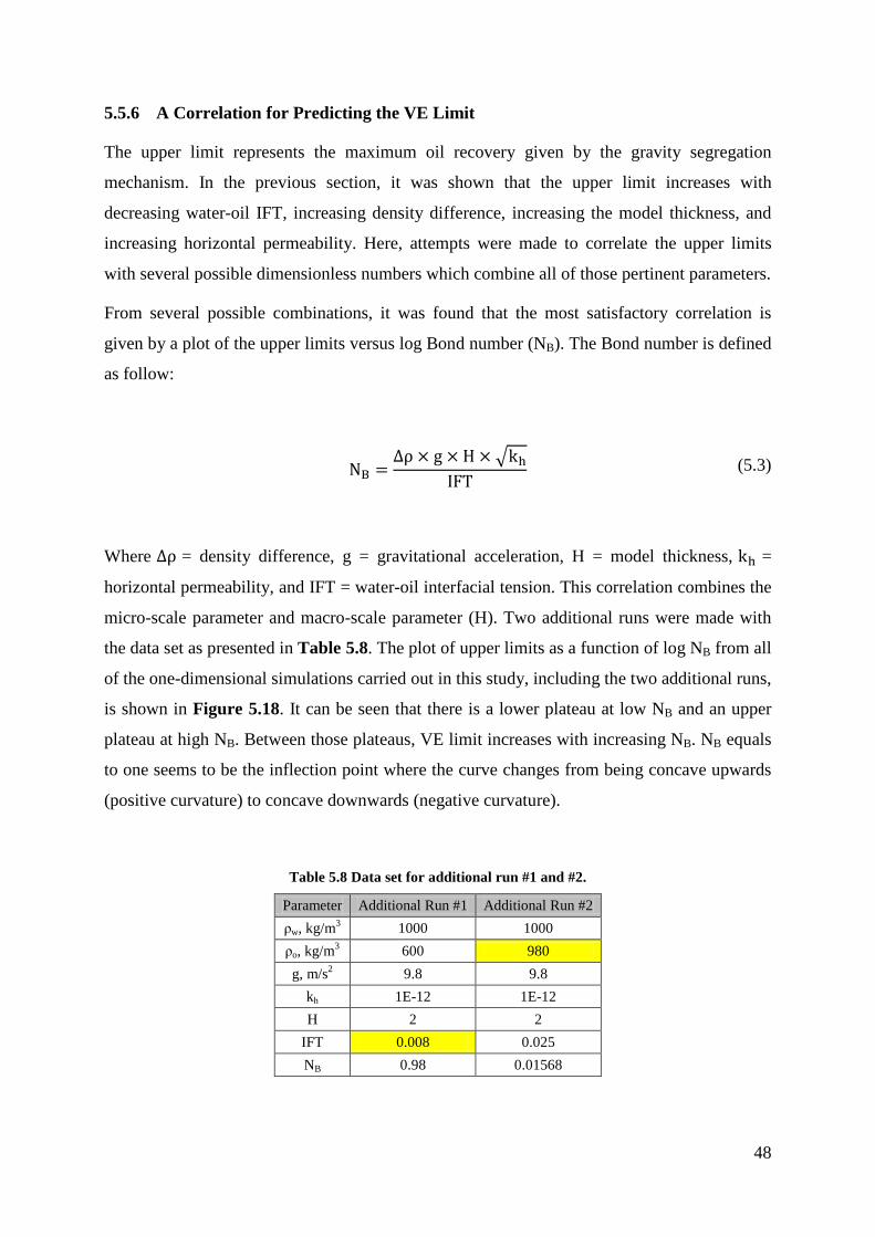
48
5.5.6 A Correlation for Predicting the VE Limit
The upper limit represents the maximum oil recovery given by the gravity segregation
mechanism. In the previous section, it was shown that the upper limit increases with
decreasing water-oil IFT, increasing density difference, increasing the model thickness, and
increasing horizontal permeability. Here, attempts were made to correlate the upper limits
with several possible dimensionless numbers which combine all of those pertinent parameters.
From several possible combinations, it was found that the most satisfactory correlation is
given by a plot of the upper limits versus log Bond number (NB). The Bond number is defined
as follow:
NB =
∆ρ × g × H × �khIFT
(5.3)
Where ∆ρ = density difference, g = gravitational acceleration, H = model thickness, kh =
horizontal permeability, and IFT = water-oil interfacial tension. This correlation combines the
micro-scale parameter and macro-scale parameter (H). Two additional runs were made with
the data set as presented in Table 5.8. The plot of upper limits as a function of log NB from all
of the one-dimensional simulations carried out in this study, including the two additional runs,
is shown in Figure 5.18. It can be seen that there is a lower plateau at low NB and an upper
plateau at high NB. Between those plateaus, VE limit increases with increasing NB. NB equals
to one seems to be the inflection point where the curve changes from being concave upwards
(positive curvature) to concave downwards (negative curvature).
Table 5.8 Data set for additional run #1 and #2.
Parameter Additional Run #1 Additional Run #2 ρw, kg/m3 1000 1000 ρo, kg/m3 600 980 g, m/s2 9.8 9.8
kh 1E-12 1E-12 H 2 2
IFT 0.008 0.025 NB 0.98 0.01568

49
Figure 5.18 VE limit as a function of NB.
If the Bond numbers are plotted against Sor, as shown in Figure 5.19, the shape of the curve
would resemble the CDC (see Figure 3.4). These results demonstrate that the Bond number
has to be increased above a critical value in order to decrease the residual oil saturation. In
this simulation model, this critical Bond number is approximately around 0.07.
Figure 5.19 Residual oil saturation as a function of NB.
0.65
0.7
0.75
0.8
0.85
0.9
0.01 0.1 1 10 100
VE L
imit
NB
Base Case, 25 dynes/cm
Base Case, 1 dynes/cm
High kv, 25 dynes/cm
High kv, 1 dynes/cm
High oil dens, 25 dynes/cm
High oil dens, 1 dynes/cm
Large Thickness, 25 dynes/cm
Large Thickness, 1 dynes/cm
Low kh, 25 dynes/cm
Low kh, 1 dynes/cm
Additional Run #1
Additional Run #2
0.1
0.15
0.2
0.25
0.3
0.35
0.01 0.1 1 10 100
S or
NB
Base Case, 25 dynes/cm
Base Case, 1 dynes/cm
High kv, 25 dynes/cm
High kv, 1 dynes/cm
High oil dens, 25 dynes/cm
High oil dens, 1 dynes/cm
Large Thickness, 25 dynes/cm
Large Thickness, 1 dynes/cm
Low kh, 25 dynes/cm
Low kh, 1 dynes/cm
Additional Run #1
Additional Run #2
Additional runs

50
6 CONCLUSIONS AND RECOMMENDATIONS
6.1 Conclusions
This simulation study enabled the following conclusions to be made.
1. Gravity segregation behind the displacement front gives positive effect on oil recovery by
accumulating the oil phase at the top of the model, thus improving the effective horizontal
oil mobility. In an ideal model, the oil recovery could be 16% higher than that would be
predicted if gravity segregation was ignored.
2. Simulations in various models indicate that reducing IFT will increase the degree of
gravity segregation, thus improving the oil recovery. The effect of reducing IFT was
found to be more significant in a thin model with low horizontal permeability, and high
density difference. However, the degree of gravity segregation is relatively insensitive to
the magnitude of the oil densities normally encountered in actual oil production
operations.
3. There is a critical velocity above which gravity segregation will not occur. Reducing the
velocity below the critical value will increase the degree of gravity segregation until an
equilibrium condition is reached.
4. The critical velocity was found to increase with increasing vertical permeability,
increasing density difference, and decreasing the model thickness.
5. The oil recovery at the equilibrium condition represents the maximum oil recovery given
by gravity segregation mechanism. It can be predicted by using one-dimensional
simulation with vertical equilibrium (VE) upscaled relative permeability curves.
6. Gravity segregation was found to occur when the dimensionless viscous-gravity forces
ratio (Rvg) is around 1. This correlation can be used to estimate the required pressure
difference or injection velocity for the gravity segregation to occur.
7. A correlation between residual oil saturation and Bond number (NB) has a similar shape as
the Capillary Desaturation Curve (CDC). There is a critical Bond number where gravity
forces starts to overcome the capillary forces and decrease the residual oil saturation.
8. Both the Rvg and NB correlations were derived using an ideal homogenous model. It may
not be applicable to heterogeneous reservoirs.
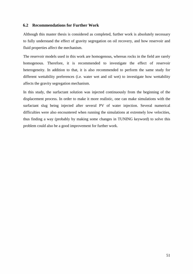
51
6.2 Recommendations for Further Work
Although this master thesis is considered as completed, further work is absolutely necessary
to fully understand the effect of gravity segregation on oil recovery, and how reservoir and
fluid properties affect the mechanism.
The reservoir models used in this work are homogenous, whereas rocks in the field are rarely
homogenous. Therefore, it is recommended to investigate the effect of reservoir
heterogeneity. In addition to that, it is also recommended to perform the same study for
different wettability preferences (i.e. water wet and oil wet) to investigate how wettability
affects the gravity segregation mechanism.
In this study, the surfactant solution was injected continuously from the beginning of the
displacement process. In order to make it more realistic, one can make simulations with the
surfactant slug being injected after several PV of water injection. Several numerical
difficulties were also encountered when running the simulations at extremely low velocities,
thus finding a way (probably by making some changes in TUNING keyword) to solve this
problem could also be a good improvement for further work.

52
REFERENCES
ECLIPSE Technical Description. (2009). Schlumberger.
(2011, May). Retrieved from U.S. Energy Information Administration: http://www.eia.gov
Agbalaka, C. D. (2008). The Effect of Wettability on Oil Recovery: A Review. SPE 114496.
Anderson, W. (1986). Wettability Literature Survey - Part 2: Wettability Measurement. JPT,
1246-1262.
Anderson, W. (December 1987c). Wettability Literature Survey – Part 6: The Effects of
Wettability on Waterflooding. JPT, 1605-1622.
Anderson, W. (November 1987b). Wettability Literature Survey – Part 5: The Effects of
Wettability on Relative Permeability. JPT, 1453-1468.
Anderson, W. (October 1987a). Wettability Literature Survey – Part 4: Effects of Wettability
on Capillary Pressure. JPT, 1238-1300.
Bardon, C. L. (October 1980). Influence of Very Low Interfacial Tensions on Relative
Permeability. SPE Journal, 391-401.
Batychy, J. M. (1978). Low Interfacial Tension Displacement Studies. Petroleum Society of
CIM 78-29-26.
Behbahani, H. B. (2004). Analysis of Imbibition in Mixed-Wet Rocks Using Pore-Scale
Modeling. SPE 90132.
Cosentino, L. (2001). Integrated Reservoir Studies. Paris: Editions Technip.
Craft, B. H. (1991). Applied Petroleum Reservoir Engineering. Englewood Cliffs, NJ:
Prentice Hall.
Donaldson, E. T. (1971). Microscopic Observations of Oil Displacement in Water-Wet and
Oil-Wet Systems. SPE 3555.
Dong, H. H. (2006). The Effect of Wettability on Oil Recovery of
Alkaline/Surfactant/Polymer Flooding. SPE 102564.
Dyke, K. (1997). Fundamentals of Petroleum. Austin, Texas: Petroleum Extension Service.
Garnes, J. M. (1990). Capillary Number Relations for Some North Sea Reservoir Sandstones.
SPE/DOE 20264.
Gilliland, H. C. (1976). A Pilot Test of Surfactant Flooding in the Big Muddy Field. SPE
5891.
Green, D. W. (1998). Enhanced Oil Recovery. Richardson, Texas: SPE.
Healy, R. R. (April 1977). Immiscible Microemulsion Flooding. SPE Journal, 129-139.
Healy, R. R. (June 1976). Multiphase Microemulsion Systems. SPE Journal, 147-160.

53
Hornof, V. M. (1987). Gravity Effects in the Displacement of Oil by Surfactant Solutions.
SPE 13573.
Hornof, V. M. (1987). Gravity Effects in the Displacement of Oil by Surfactant Solutions.
SPE 13573.
Kolnes, J. (1992). Surfactant Flooding Displacement Mechanisms. In S. K. Skjæveland,
SPOR Monograph: Recent Advances in Improved Oil Recovery Methods for North Sea
Sandstone Reservoirs (pp. 239-243). Stavanger: NPD.
Lake, L. (1989). Enhanced Oil Recovery. Englewood Cliffs, NJ: Prentice Hall Inc.
Lohne, A. V. (2007). Flow 2D User’s Manual. Stavanger: IRIS.
Melrose, J. B. (October-December 1974). Role of Capillary Forces in Determining
Microscopic Displacement Efficiency for Oil Recovery by Waterflooding. JCPT, 54-
62.
Morrow, N. (July-September 1979). Interplay of Capillary, Viscous, and Buoyancy Forces in
the Mobilization of Residual Oil. JCPT, 35-46.
Morrow, N. (July-September 1979). Interplay of Capillary, Viscous, and Buoyancy Forces in
the Mobilization of Residual Oil. JCPT, 35-46.
Morrow, N. S. (1981). Effect of Viscous and Buoyancy Forces on Non-Wetting Phase
Trapping in Porous Media. In O. Shah, Surface Phenomena in Enhanced Oil Recovery
(pp. 387-411). New York: Plenum Press.
Ottewill, R. (1984). Surfactants. San Fransisco: Academic Press.
Rao, D. G. (June 1992). The Influence of Reservori Wettability on Waterflood and Miscible
Flood Performance. JCPT, 47-55.
Raza, S. T. (April 1968). Wettability of Reservoir Rocks and Its Evaluation. Prod. Monthly,
2-7.
Salathiel, R. (October 1973). Oil Recovery by Surface Film Drainage in Mixed Wettability
Rocks. JPT, 1216-1224.
Schester, D. Z. (1991). Capillary Imbibition and Gravity Segregation in Low IFT Systems.
SPE 22594.
Wood, A. W. (1991). Determining Effective Residual Oil Saturation for Mixed Wettability
Reservoirs: Endicott Field, Alaska. SPE 22903.

54
APPENDICES
A Eclipse Input Data for Base Case -------
RUNSPEC
-------
TITLE
BASE CASE MODEL
DIMENS
100 1 20 /
NONNC
OIL
WATER
SURFACT
METRIC
TABDIMS
2 1 100 20 1 /
ENDSCALE
/
WELLDIMS
2 50 1 2 /
START
7 MAY 2011 /
NSTACK
50 /
--NOSIM
----
GRID
----
INIT
DXV
100*5 /
DYV
1*5 /
DZ

55
2000*0.1 /
PERMX
2000*1000 /
PERMY
2000*1000 /
PERMZ
2000*250 /
PORO
2000*0.25 /
TOPS
100*2500 /
JFUNC
--DYNE.PER.CM
WATER 25 /
RPTGRID
/
-----
PROPS
-----
SWFN
--SW KRW J
0.148000 0.00000000 200.0000
0.149590 0.00000001 23.83791
0.153375 0.00000002 6.147762
0.160945 0.00000004 2.258275
0.168515 0.00000009 1.309519
0.176085 0.00000021 0.888995
0.183655 0.00000036 0.653511
0.191225 0.00000054 0.503619
0.198795 0.00000081 0.400102
0.206365 0.00000121 0.324441
0.213935 0.00000176 0.266779
0.221505 0.00000255 0.221397
0.229075 0.00000369 0.184753
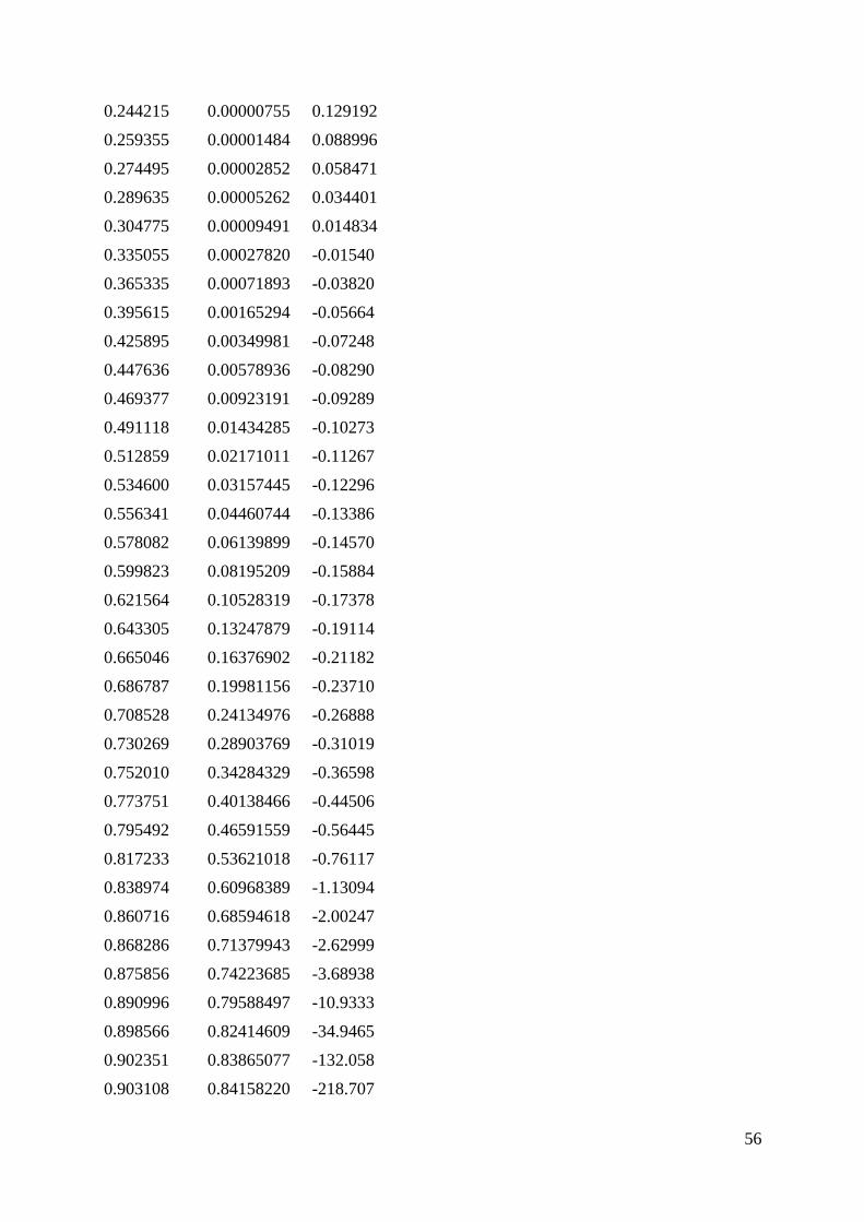
56
0.244215 0.00000755 0.129192
0.259355 0.00001484 0.088996
0.274495 0.00002852 0.058471
0.289635 0.00005262 0.034401
0.304775 0.00009491 0.014834
0.335055 0.00027820 -0.01540
0.365335 0.00071893 -0.03820
0.395615 0.00165294 -0.05664
0.425895 0.00349981 -0.07248
0.447636 0.00578936 -0.08290
0.469377 0.00923191 -0.09289
0.491118 0.01434285 -0.10273
0.512859 0.02171011 -0.11267
0.534600 0.03157445 -0.12296
0.556341 0.04460744 -0.13386
0.578082 0.06139899 -0.14570
0.599823 0.08195209 -0.15884
0.621564 0.10528319 -0.17378
0.643305 0.13247879 -0.19114
0.665046 0.16376902 -0.21182
0.686787 0.19981156 -0.23710
0.708528 0.24134976 -0.26888
0.730269 0.28903769 -0.31019
0.752010 0.34284329 -0.36598
0.773751 0.40138466 -0.44506
0.795492 0.46591559 -0.56445
0.817233 0.53621018 -0.76117
0.838974 0.60968389 -1.13094
0.860716 0.68594618 -2.00247
0.868286 0.71379943 -2.62999
0.875856 0.74223685 -3.68938
0.890996 0.79588497 -10.9333
0.898566 0.82414609 -34.9465
0.902351 0.83865077 -132.058
0.903108 0.84158220 -218.707

57
0.903865 0.84452387 -470.499
0.905000 0.84747583 -600.000
/
0.148000 0.00000000 200.0000
0.149590 0.00000001 23.83791
0.153375 0.00000002 6.147762
0.160945 0.00000004 2.258275
0.168515 0.00000009 1.309519
0.176085 0.00000021 0.888995
0.183655 0.00000036 0.653511
0.191225 0.00000054 0.503619
0.198795 0.00000081 0.400102
0.206365 0.00000121 0.324441
0.213935 0.00000176 0.266779
0.221505 0.00000255 0.221397
0.229075 0.00000369 0.184753
0.244215 0.00000755 0.129192
0.259355 0.00001484 0.088996
0.274495 0.00002852 0.058471
0.289635 0.00005262 0.034401
0.304775 0.00009491 0.014834
0.335055 0.00027820 -0.01540
0.365335 0.00071893 -0.03820
0.395615 0.00165294 -0.05664
0.425895 0.00349981 -0.07248
0.447636 0.00578936 -0.08290
0.469377 0.00923191 -0.09289
0.491118 0.01434285 -0.10273
0.512859 0.02171011 -0.11267
0.534600 0.03157445 -0.12296
0.556341 0.04460744 -0.13386
0.578082 0.06139899 -0.14570
0.599823 0.08195209 -0.15884
0.621564 0.10528319 -0.17378
0.643305 0.13247879 -0.19114

58
0.665046 0.16376902 -0.21182
0.686787 0.19981156 -0.23710
0.708528 0.24134976 -0.26888
0.730269 0.28903769 -0.31019
0.752010 0.34284329 -0.36598
0.773751 0.40138466 -0.44506
0.795492 0.46591559 -0.56445
0.817233 0.53621018 -0.76117
0.838974 0.60968389 -1.13094
0.860716 0.68594618 -2.00247
0.868286 0.71379943 -2.62999
0.875856 0.74223685 -3.68938
0.890996 0.79588497 -10.9333
0.898566 0.82414609 -34.9465
0.902351 0.83865077 -132.058
0.903108 0.84158220 -218.707
0.903865 0.84452387 -470.499
0.905000 0.84747583 -600.000
/
SOF2
--SO KRO
0.09500 0.00000000
0.12528 0.00000077
0.15556 0.00000491
0.18584 0.00002617
0.21612 0.00011603
0.2464 0.00042824
0.27668 0.00131584
0.30696 0.00336597
0.33724 0.00716820
0.36752 0.01275780
0.3978 0.02070515
0.42808 0.03237853
0.45836 0.04878788
0.48864 0.07083417

59
0.51892 0.09909457
0.5492 0.13357739
0.57948 0.17349708
0.60976 0.21713381
0.64004 0.26475376
0.67032 0.32144566
0.7006 0.38839826
0.73088 0.46703697
0.76116 0.55889411
0.79144 0.66559810
0.82172 0.78885812
0.8520 0.93044349
/
0.09500 0.00000000
0.12528 0.00000077
0.15556 0.00000491
0.18584 0.00002617
0.21612 0.00011603
0.2464 0.00042824
0.27668 0.00131584
0.30696 0.00336597
0.33724 0.00716820
0.36752 0.01275780
0.3978 0.02070515
0.42808 0.03237853
0.45836 0.04878788
0.48864 0.07083417
0.51892 0.09909457
0.5492 0.13357739
0.57948 0.17349708
0.60976 0.21713381
0.64004 0.26475376
0.67032 0.32144566
0.7006 0.38839826
0.73088 0.46703697

60
0.76116 0.55889411
0.79144 0.66559810
0.82172 0.78885812
0.8520 0.93044349
/
PVTW
--P FVF COMP VISC VISCOSIBILITY
250 1 0 0.3 0 /
PVDO
--P FVF VISC
250 1.0000 0.5
50000 0.9999 0.5 /
ROCK
--P COMP
250 1E-9 /
DENSITY
--OIL WATER GAS
600 1000 10 /
SURFVISC
--CONC VISC
0 0.3
10 0.3 /
SURFST
--CONC IFT.NEWTON.PER.M
0.0 0.025
0.5 0.001
1.5 0.0001
3.0 0.00001
6.0 0.000001
10 0.000001 /
SURFCAPD
--LOGNC 1=MISC 0=IMMISC
-9.0 0.0
-4.5 0.0
-2.0 1.0

61
10 1.0 /
-9.0 0.0
-4.5 0.0
-2.0 1.0
10 1.0 /
RPTPROPS
'SURFVISC' /
-------
REGIONS
-------
SATNUM
2000*1 /
SURFNUM
2000*2 /
RPTREGS
/
--------
SOLUTION
--------
EQUIL
--DEPTH BHP WOC PC
2500 250 2510 5 /
RPTSOL
'PRES' 'SOIL' 'SWAT' 'RESTART=1' 'SURFBLK' 'FIPSURF=2' /
-------
SUMMARY
-------
FOE
--RECOVERY FACTOR
FOPR
--FIELD.OIL.PROD.RATE
FOPT
--FIELD.OIL.PROD.TOTAL
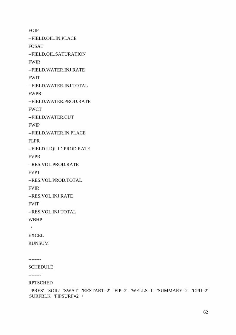
62
FOIP
--FIELD.OIL.IN.PLACE
FOSAT
--FIELD.OIL.SATURATION
FWIR
--FIELD.WATER.INJ.RATE
FWIT
--FIELD.WATER.INJ.TOTAL
FWPR
--FIELD.WATER.PROD.RATE
FWCT
--FIELD.WATER.CUT
FWIP
--FIELD.WATER.IN.PLACE
FLPR
--FIELD.LIQUID.PROD.RATE
FVPR
--RES.VOL.PROD.RATE
FVPT
--RES.VOL.PROD.TOTAL
FVIR
--RES.VOL.INJ.RATE
FVIT
--RES.VOL.INJ.TOTAL
WBHP
/
EXCEL
RUNSUM
--------
SCHEDULE
--------
RPTSCHED
'PRES' 'SOIL' 'SWAT' 'RESTART=2' 'FIP=2' 'WELLS=1' 'SUMMARY=2' 'CPU=2' 'SURFBLK' 'FIPSURF=2' /

63
WELSPECS
--WELL GROUP I J DEPTH PHASE
'PRO' 'G' 100 1 2500 'OIL' /
'INJ' 'G' 1 1 2500 'WAT' /
/
COMPDAT
--WELL I J K1 K2 OPEN.CLOSE 1* WELL.CON.FACTOR RW
'PRO' 100 1 1 20 'OPEN' 1* 34.108 /
'INJ' 1 1 1 20 'OPEN' 1* 34.108 /
/
WCONPROD
--WELL OPEN.CLOSE CONTROL 4* RESV BHP.LOWER.LIMIT
'PRO' 'OPEN' 'BHP' 5* 200 /
/
WCONINJE
--WELL PHASE OPEN.CLOSE CONTROL RATE RESV BHP.UPPER.LIMIT
'INJ' 'WAT' 'OPEN' 'RESV' 1* 5 50000 /
/
WSURFACT
--WELL CONC
'INJ' 0 /
/
TUNING
0.001 3 0.00001 1* 1.5 /
1* 1E-5 1* 1E-7 /
100 1* 100 1* 100 /
TSTEP
1250 /
END

64
B Flow2D Upscaling Input Data for Base Case runsect
*IDENTIFICATION OF THE RUN (CASE DESCRIPTION).
--------------------------------------------------------------------------
--------------------------------------------------------------------------
title
'Homogeneous model: 500m×2m' /
ruNflags
2 1 1 0 1 /
rateflag
0 /
sourcedim
100 20 1 1 0 0 /
phases
1 1 0 /
nrock
1 /
nstack
30 /
pause
1 /
-----------------------------------------------------------------------
gridsect
-----------------------------------------------------------------------
orientation
90 0 /
permx
1 / Darcy
permy
0.25 /
poro
15000*0.25 /
dx
100*500 / cm

65
dy
20*10 / cm
-----------------------------------------------------------------------
propsect
-----------------------------------------------------------------------
density
0.6 1 0.010 / (g/ml)
ift
25 1 / mN/m=dynes/cm
viscosity
0.5 0.3 0.0289 / o-w-g
jscale
1 /
krtab1
1 1 2 3 1 / rock 1
include "incl/relp_mixed-wet_1.txt" /
/
pctab1
1 1 3 /
include "incl/Pc_imb_mixed-wet_1.txt" /
/
swco
1 1 1 /
-----------------------------------------------------------------------
compsect
-----------------------------------------------------------------------
PcwLIST
40 2 2 /
-2.5 -1.25 /
1.25 2.5 /
newttol
500 0.01 0.00001 /
dtcalc

66
0.2 0.0001 1.1 0.75 1 0 0 /
dttol
1e-10 0.0001 2 3 200 /
lintol
500 1e-10 /
confact
1e6 10000 1 1 /
solver
1 2 /
upstream
1 /
end

67
C Production and Injection Well Bottomhole Pressure for All 1D Simulations
kv = 250 md, kh = 1000 md, ρo = 600 kg/m3, H = 2 m IFT = 25 dynes/cm IFT = 1 dynes/cm
RF, % WBHP-I WBHP-P RF, % WBHP-P WBHP-I 0.73154 202.1 200 0.81905 201.3 200 0.72681 222 200 0.77695 216.4 200 0.70495 455 200 0.72128 428 200 0.68982 3099 200 0.6906 3077.4 200 0.68902 29415.3 200 0.68902 29414.9 200
kv = 1000 md, kh = 1000 md, ρo = 600 kg/m3, H = 2 m
IFT = 25 dynes/cm IFT = 1 dynes/cm RF, % WBHP-I WBHP-P RF, % WBHP-P WBHP-I
0.73202 202.1 200 0.83557 201.3 200 0.73092 221.4 200 0.80598 214.1 200 0.72027 428.5 200 0.75491 385.7 200 0.69514 2958.8 200 0.70089 2832.4 200 0.68911 29385.8 200 0.6893 29329 200
kv = 250 md, kh = 250 md, ρo = 600 kg/m3, H = 2 m
IFT = 25 dynes/cm IFT = 1 dynes/cm RF, % WBHP-I WBHP-P RF, % WBHP-P WBHP-I
0.70729 210 200 0.8162 205.4 200 0.7059 301.8 200 0.77656 265.7 200
0.69771 1279.5 200 0.72103 1112.6 200 0.68927 11828.7 200 0.69027 11716.5 200 0.68883 116974.6 200 0.68883 116972.6 200
kv = 250 md, kh = 1000 md, ρo = 850 kg/m3, H = 2 m
IFT = 25 dynes/cm IFT = 1 dynes/cm RF, % WBHP-I WBHP-P RF, % WBHP-P WBHP-I
0.70072 202.6 200 0.79849 201.5 200 0.69893 226.9 200 0.75324 218.8 200 0.69185 484.3 200 0.6997 465.7 200 0.68917 3118.2 200 0.68938 3112 200 0.68902 29415.7 200 0.68902 29415.7 200
kv = 250 md, kh = 1000 md, ρo = 600 kg/m3, H = 20 m
IFT = 25 dynes/cm IFT = 1 dynes/cm RF, % WBHP-I WBHP-P RF, % WBHP-P WBHP-I
0.77216 201.7 200 0.77777 201.6 200 0.71957 223 200 0.72145 222.8 200 0.69051 487.9 200 0.69065 487.6 200 0.68916 3118.7 200 0.68916 3118.8 200 0.68901 29416.5 200 0.68901 29416.5 200
Top Related