


Languages
Pages
Legal

December 2004 Productivity, Taxes and Hours Worked in Spain: 1970–2000 Juan C. Conesa Universitat Pompeu Fabra, Centre de Referència d’Economia Analítica, Universitat de Barcelona, and Centre de Recerca en Economia del Benestar Timothy J. Kehoe University of Minnesota and Federal Reserve Bank of Minneapolis Abstract _________________________________________________________________
In 1975 hours worked per adult were higher in Spain than in the US, one decade later they
were 40 percent smaller. This paper quantitatively assesses the impact of the evolution of
TFP and taxes on the evolution of aggregate hours worked in Spain. Solow decomposition
shows that the sharp decrease in hours worked per adult is responsible for the negative
comovement of TFP and output per adult. We show that as mcu as 80 percent of the
decrease in hours worked can be accounted for by the evolution of taxation in an otherwise
standard neoclassical growth model. Finally, we provide a comparison with the experience
of France over the same period and show that the model fits well the French experience
over the same time period.
_________________________________________________________________________
*This work has benefited from outstanding research assistance by Kim Ruhl and from comments by participants at seminars at the Federal Reserve Bank of Minneapolis, Florida State University, Universitat de Barcelona, Universitat Pompeu Fabra, Universitat Rovira i Virgili, and 2003 Workshop of the Jornadas Béticas de Macroeconomía Dinámica. Conesa acknowledges financial support from the Fundación Ramón Areces, Ministerio de Ciencia y Tecnología, SEC2003-06080, and the Generalitat de Catalunya, SGR00-016.
1. Introduction What has driven output growth and fluctuations in Spain over the past three
decades? What has been the impact of the evolution of taxes on aggregate hours worked
and output? We answer these questions using the methodology developed by Cole and
Ohanian (1999) and Kehoe and Prescott (2002) to study great depressions. This
methodology relies on growth accounting and a simple general equilibrium growth model.
Our growth accounting indicates that, over the period 1970 to 2000, the major factor in
determining economic fluctuation in Spain has been fluctuations in aggregate hours
worked, rather than fluctuations in productivity growth or in capital accumulation. Our
applied general equilibrium analysis indicates that most of the fluctuations in hours worked
can be accounted for by changes in taxes. In particular, the model accounts for more than
70 percent of the sharp decline in hours worked over the period the evolution of aggregate
hours worked in Spain is consistent with the evolution of taxes from a neoclassical growth
perspective. Moreover the sharp decrease in hours worked happened over a time period
with high total factor productivity growth. As a way of comparison, we use the same
methodology for the French case and we find that the model economy is consistent with the
data for the French economy as well. Again, it is the evolution of taxes and not lack of
productivity growth what drives hours worked and output per capita.
The methodology used is the one introduced in Kehoe and Prescott (eds., 2002),
following the steps of a similar methodology proposed in Cole and Ohanian (1999) to the
study of the US Great Depression.
In the first step, growth accounting is used to quantify the contribution of Total
Factor Productivity (from now on, we refer to it as TFP), capital deepening and aggregate
hours worked for the dynamics of output relative to trend. Next, a standard neoclassical
growth model is constructed, where a stand-in household is choosing hours worked,
consumption and capital holdings, taking as given the deterministic evolution of TFP and
tax rates. Such a methodology provides a quantitative tool, at the same time that identifies
the relevant margins for potential candidate explanations.
Prior to 1975 TFP and output per working age person perfectly comoved in Spain.
However, after 1975 this is not the case anymore. The reason is the beginning of a
generalized process of decreasing aggregate hours worked. That observation is also present

3
in the French economy and is in sharp contrast with the US experience, where hours
worked per adult have been roughly constant, and even increasing during the last fifteen
years. Spain is just an extreme case of “European-like” labor market dynamics. The
comparison with France shows that the decrease in hours worked started later in time (1975
as compared to the late sixties), but was quantitatively sharper.
Such differential labor market experiences between US and Europe have been
extensively studied in the literature. Most of the literature in this research area has focused
on the impact of differences in labor market institutions. Bentolila and Bertola (1990),
Blanchard and Jimeno (1995) or Blanchard and Summers (1986) among others, focus on
the role of institutions and labor market restrictions. Sargent and Ljungqvist (1999, 2002)
focus on the interaction between shocks and institutions in a labor search model. Prescott
(2002), however, argues that differential taxation alone might account for the differences in
the current level of aggregate hours worked between France and the US. To our knowledge,
though, ours is the first attempt to quantify the implications of the evolution of taxes for the
evolution of aggregate hours worked.
Our analysis shows that the evolution of the taxation of consumption and factor
earnings can account for 80% of the secular trend decrease in hours worked in Spain and
virtually all of the decrease in France. We show that the behaviour of aggregate hours
worked is in line with the predictions of standard neoclassical theory, in contrast with most
theoretical work relying in differences in labor market institutions. Of course our exercise is
silent about the distribution of aggregate hours worked within the working age population.
Also, the exercise proposed allows us to identify time periods in which data deviates from
theory in a quantitatively important way. We want to identify these episodes, since they
suggest avenues for future research.
Several papers have tried to understand whether Spain displays differential features
in terms of employment dynamics than other European economies. Our exercise seems to
agree with several other papers that find the Spanish economy much more in line with other
economies than other authors have tried to argue. In particular, Zilibotti and Marimon
(1998) find that conditioning for initial sectoral composition of output there is no
substantial difference in Spanish employment dynamics relative to the rest of European
economies. Also, Jimenez-Martin and Sanchez-Martin (2003) contribute to understanding

4
the role of retirement incentives provided by the Spanish Social Security system, which is a
non-trivial component of the fall in aggregate hours worked.

5
2. The Growth Accounting Exercise
In order to construct the growth accounting exercise we use National Accounts using the
System of National Accounts (SNA93) and data on hours worked per worker and
employment rates by the corresponding country Labor Force Surveys.
We construct a series of capital by using the Perpetual Inventory Method given the
available series of investment (starting back in 1954) and a value for the constant
depreciation rate, chosen to be 0.0453δ = . This value is chosen to be consistent with the
ratio of depreciation to GDP observed in the data.
The standard growth accounting is done as in Kehoe and Prescott (2002), by using an
aggregate production function of the form:
1t t t tY A K Lα α−=
where tA is TFP, and tK and tL are the capital and labor inputs respectively.
Dividing by working-age population, tN , we can decompose the evolution of output
according to the following expression:
1 1
1t t tt
t t t
Y K LAN Y N
αα
α−
−⎛ ⎞ ⎛ ⎞
= ⎜ ⎟ ⎜ ⎟⎝ ⎠ ⎝ ⎠
Assigning a value for the capital share α we are ready to perform our decomposition. We
measure directly α from the data and obtain a value of 0.31. Our estimate is slightly higher
than the estimated value in Gollin (2002), who argues for a common across countries
capital share of income = 0.3α . Notice that this number is very similar to the EU estimate
of 0.305 (see European Economy (1994)).
Along a balanced growth path the capital-output ratio, /t tK Y , and hours worked per
working-age person, /t tL N , are constant over time. Therefore output per working-age
6
person should grow at rate implied by the TFP factor, 1
1tA α− .
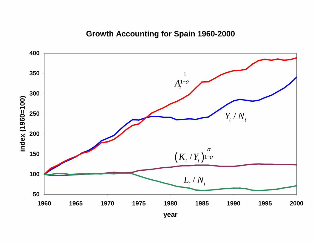
First, we report the growth accounting exercise for the US in Figure 1. Notice the contrast
with the case of Spain, as reported in Figure 2. Clearly, after 1975 Spain deviates from
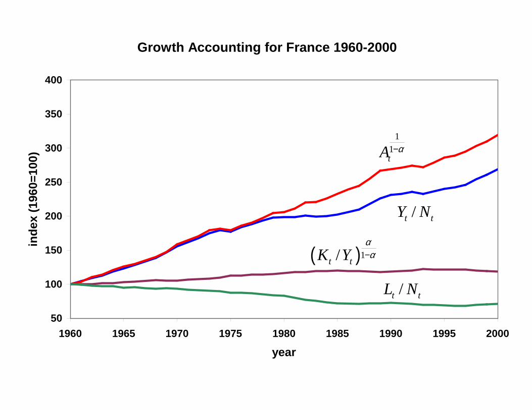
balanced growth path. A similar conclusion can be reached for the case of France, reported
in Figure 3.
Notice that, while in the period 1960–1975, the data seems to indicate a Balanced Growth
Path for the case of Spain, subsequent to 1975 the TFP factor and output per adult start
diverging. The reason is the dramatic fall in aggregate hours worked.
Figure 4 displays the evolution of aggregate hours worked. Notice that the fall in aggregate
hours worked starting in 1975 is due to both a fall in hours worked per worker and a fall in
employment rates. However, the main focus of this paper is to understand the contribution
of the evolution of taxes for this observed fall in aggregate hours worked, but not on its
distribution across the population.
Such a sharp decline in aggregate hours worked is in line with the economic experiences of
other European economies. It is illustrative to compare the evolution of hours worked in
Spain with those in France and the US. This comparison is reported in Figure 5.
Notice that France and Spain have experienced a similar drop in hours worked between
1960 and 2000. However, the French case has been a more continuous and smooth process
taking place since 1960, while the Spanish experience was concentrated in the decade
between 1975 and 1985. Nevertheless, the French economy experience is similar to that of
Spain, in the sense that the deviations of output relative to productivity are generated by
falling hours worked, see Figure 3.
3. The Theoretical Framework
The simplest theoretical framework one could write is one in which a stand-in infinitely-
lived consumer is going to choose sequences of consumption, hours worked and capital,
taking as given the evolution of TFP and taxes. The production side of the economy takes
place through a stand-in producer operating the aggregate technology taking competitive
7
prices as given. Finally, there is a government that levies proportional taxes on
consumption, labor earnings and capital earnings, and uses the proceeds to finance a lump-
sum transfer to the consumers in a balanced budget fashion. We will consider 1970 as our
starting point, five years before the changes which constitute the main object of this paper
take place.
In such a framework the stand-in consumer solves the following maximization problem:
1970
max [ log (1 ) log( )]tt t tt
C N h Lβ γ γ∞
=+ − −∑
1s.t. (1 )
(1 ) (1 )( ) .
ct t t t
kt t t t t t t
C K K
w L r K T
τ
τ τ δ++ + −
= − + − − +
1970 1970K K=
Here tN denotes the number of working-age population in the economy and h denotes the
yearly disposable time endowment of each individual. The choice variables are then
sequences of aggregate consumption, aggregate capital stock and aggregate hours worked,
denoted respectively by , ,t t tC K L . In Section 8 we provide a sensitivity analysis with
respect to the preferences specification, as well as with respect to the assumption that all tax
proceeds are lump-sum rebated to the consumers.
For each period the resource constraint in this economy is given by:
11 (1 ) , 1970,...t t t t t tC K K A K L tα αδ −++ − − = =
And the government budget constraint implies:
( ) , 1970,...c kt t t t t t t t tC w L r K T tτ τ τ δ+ + − = =
The problem of the stand-in producer can be characterized by the following pricing rules
for both factors of production:
8
1 1
(1 )
, 1970,...t t t t
t t t t
w A K L
r A K L t
α α
α α
α
α δ
−
− −
= −
= − =
Our benchmark specification implies that all tax proceeds are rebated to the consumer in a
lump-sum fashion.1 This is equivalent to viewing government expenditure as a perfect
substitute for private consumption, and it is a reasonable abstraction as long as tax proceeds
are mainly used to finance transfers to consumers (social security pensions, unemployment
insurance,…) or to finance publicly provided consumption goods and services (health care,
education,…) that could alternatively be provided through the private sector. In fact,
looking at the composition of government expenditure we find that in the year 1996 the
sum of pensions, healthcare, unemployment insurance and education in Spain amounted to
63% of the government outlays (25% of GDP).
Notice that this assumption is not neutral in determining the implication of taxes for hours
worked, since it generates a much bigger response of hours worked to changes in taxes. See
Prescott (2002) for a discussion of this issue. In Section 8 we provide a sensitivity analysis
with respect to this issue. In particular, we go to the other extreme and explore the
hypothesis that all government consumption is wasted or alternatively finances the
provision of public goods that enter separably in the utility function.
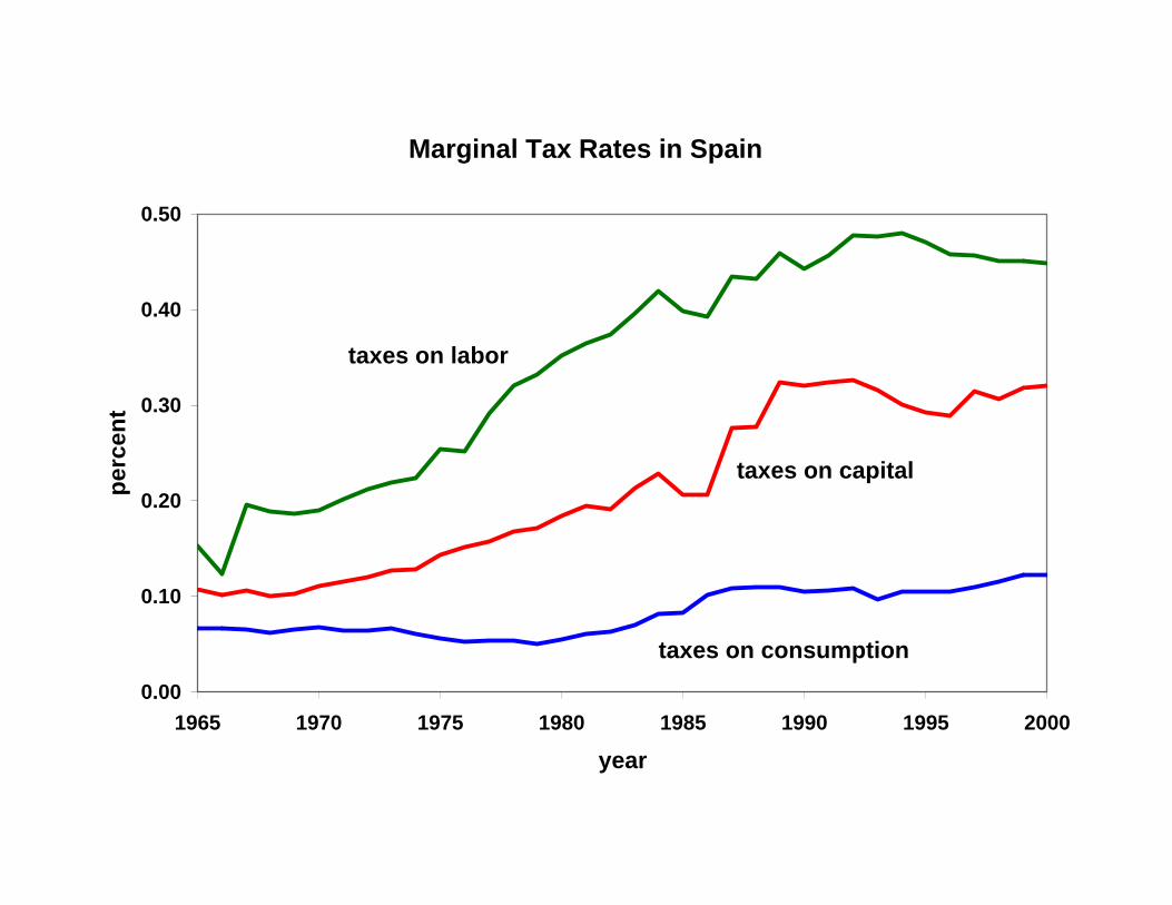
4. The Evolution of Effective Tax Rates
In order to obtain estimates of the evolution of effective marginal tax rates we use the same
methodology proposed in Mendoza et al. (1994). However, there are two main differences;
first, we attribute a fraction of household’s non-wage income to labor income; second, we
measure marginal as compared to average tax rates.
Estimating the effective marginal tax rates requires taking into account the progressivity of
income taxes. Taxation of labor earnings can be decomposed into income taxation and
1 A fraction of the tax proceeds, in Spain between 18% and 24.5% depending of the year, are lump-sum rebated through the progressivity of income taxation. Since average tax rates are smaller than marginal tax rates, we should tax at marginal rates and then have lump-sum tax rebates.

9
payroll taxes (mainly social security contributions, that are roughly proportional). Provided
that the relevant figure in terms of the distortionary implications is the marginal and not the
average tax rate, we adjust our tax estimates for both capital and labor income. Calonge and
Conesa (2003) have estimated an effective income tax function, as the one proposed in
Gouveia and Strauss (1994), for the Spanish economy using disaggregated data taken
directly from tax returns. They report that the aggregate marginal tax rate in Spain
(computed as the increase in tax revenues if everybody’s income were to increase by 1
percentage point, 26.5%) is 1.83 times bigger than the aggregate average tax rate (total tax
revenues divided by total income, 14.5%).
Hence, we adjust by 83% the taxation of households income in order to compute effective
marginal tax rates. Our final estimates are reported in Figure 6.
For a more detailed explanation of the tax estimates see Appendix A.
5. Numerical Experiment and Calibration
In the experiment we perform our theoretical economy will determine the equilibrium
evolution of the endogenous variables, given the initial capital stock in 1970 as measured in
the data. Our theoretical economy will react to the evolution of the exogenous variables,
which are the evolution of TFP as measured in the growth decomposition exercise, the
evolution of the tax rates as estimated from the data and the evolution of the working-age
population as measured in the data. Then, we will compare the evolution of the main
aggregate variables implied by the model with those observed in the data.
In order to determine the value of the disposable time endowment of individuals, h , we
assume that each adult has a time endowment of 100 hours a week.
Next, we need to assign values to all the parameters in the model.
The depreciation rate δ is chosen so that the ratio of depreciation to GDP coincides with
that observed in the data on average between 1970 and 2000. Therefore, we choose
0.0453δ = so that we obtain 2000
1970/ 31 0.142t
tt
KY
δ=
=∑ .
Our estimate of the capital share in Spain is 0.31. This estimate is obtained by using the
same national accounting data as the one used for the TFP accounting exercise and for the

10
estimation of the marginal tax rates.
In order to calibrate the preference parameters we use the first order conditions from the
household problem and the data observations for the period 1970-1974 (those are the years
for which we have complete data and are prior to the phenomenon we are interested in: the
sharp fall in hours worker starting in 1975). Deriving the two first order conditions and
rearranging we can write the value of the preference parameters as a function of data
observations:
1 1(1 ) 1(1 ) 1 (1 )( )
ct t
c kt t t t
CC r
τβτ τ δ+ ++
=+ + − −
(1 )(1 ) (1 ) ( )
ct t
ct t t t t t
CC w N h L
τγτ τ
+=
+ + − −
Using these two conditions and actual data from 1970-1974 we could compute a vector of
the parameters β and γ . The parameters we assign to our economy are the average of
these vectors.
Given that our goal is to quantify the implications of the evolution of taxes we will perform
two experiments. The first one will determine the evolution of our theoretical economy if
taxes had stayed constant at their initial level in 1970. The second experiment will
determine the evolution of the theoretical economy considering the evolution observed for
the tax variables. Then, we will compare both outcomes.
Notice then that the right parameterization will depend crucially on the assumption about
the evolution of taxes corresponding to these two experiments, yielding two different pairs
of parameters.
For the case in which we assume constant taxes at the 1970 level we find the following
parameter values: 0.9790β = , 0.3311γ = . When taxes are set equal to the actual estimated
values we find: 0.9791β = , 0.3365γ = .

11
6. The Results
Figure 7 illustrates the importance of taking into account the evolution of tax rates for
understanding the evolution of the Spanish economy during the last three decades. The
base-case model economy predictions are much more in line with the data than those
implied by the evolution of TFP alone, ignoring the evolution of taxes.
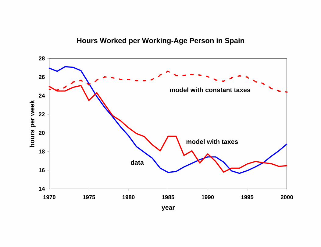
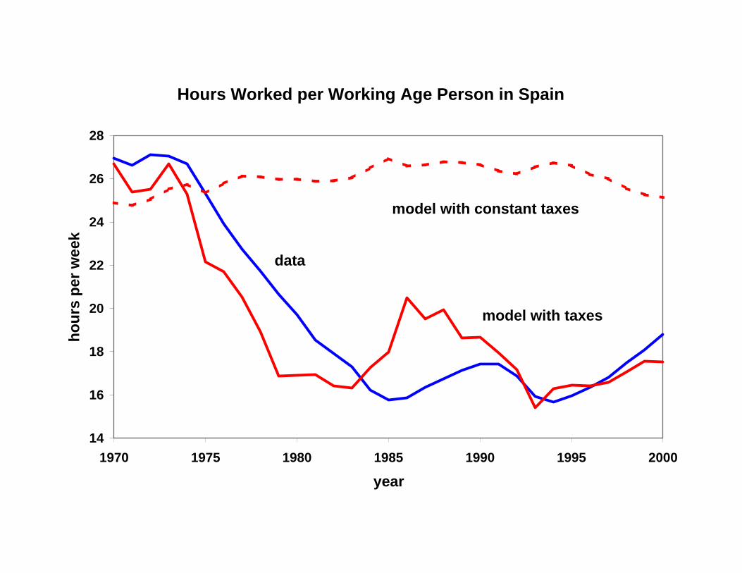
The model with taxes accounts for a sizeable fall in hours worked, see Figure 8. In fact, the
order of magnitude of this fall is captured well in the model economy: between 1974 and
1994 (the time with the lowest value) hours worked per working-age person fall 41 percent
in the data and 31 percent in the model. Nevertheless, the fall between 1974 and 1985 is not
as sharp in our base-case model economy as compared to the data. Also, it fails to account
for the recovery experienced by hours worked since 1994. In fact, several labor market
reforms have taken place since 1994 and might be responsible for this deviation of the
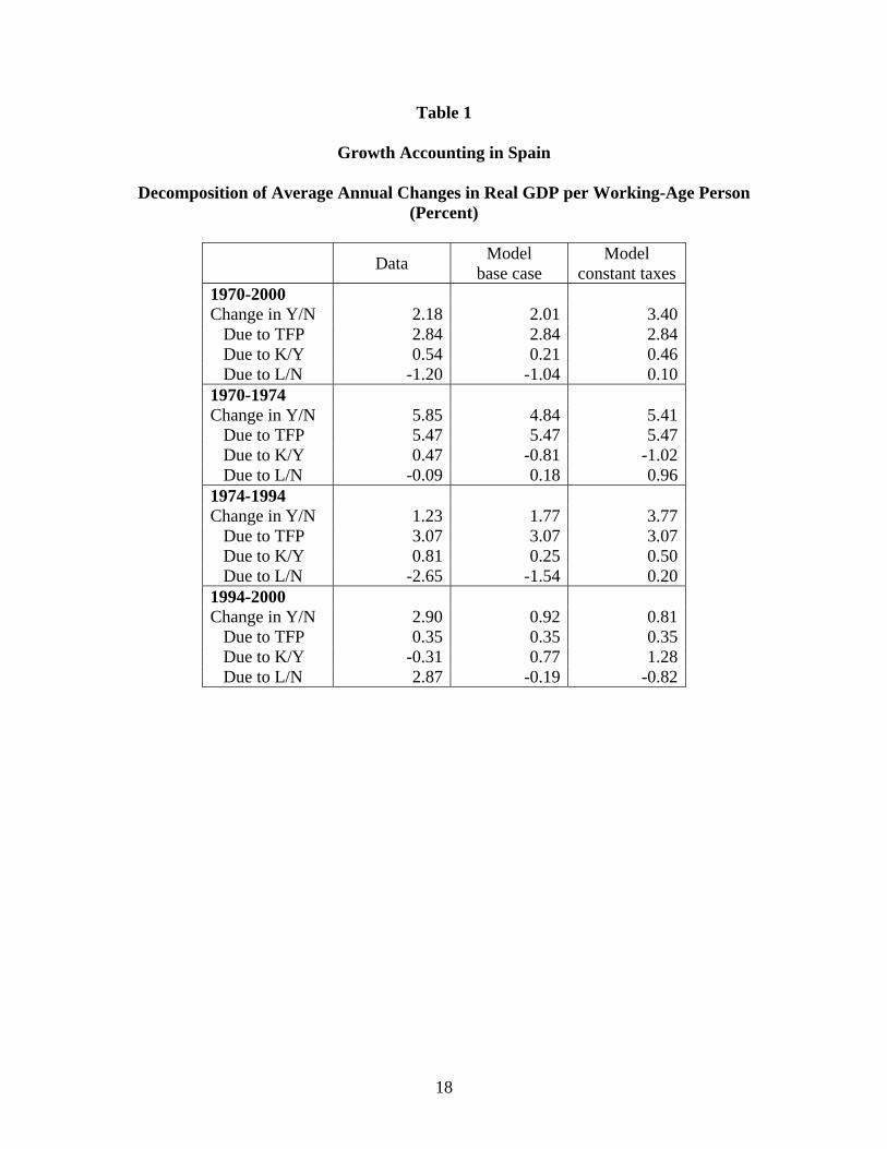
model relative to data. Table 1 shows for different subperiods the contribution of the
different components of GDP. It clearly shows how the model is not able to account for the
evolution of hours worked in the second part of the nineties, while the base case model
does reasonably well in previous periods. This shows that the labor market reforms that
were undertaken in the mid nineties have had a quantitative impact.
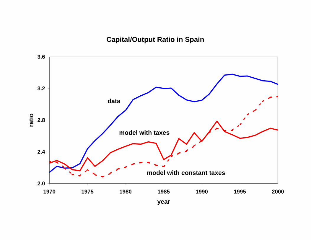
Finally, notice that the model predictions regarding capital deepening fall short of the data
experience as shown in Figure 9. Our model represents a closed economy, while capital
inflows, together with a general process of financial liberalization, might have played an
important role in capital deepening for the Spanish economy. The exercise suggests that the
evolution of taxation has not had a quantitatively important impact on that margin.
Nevertheless, our exercise shows that the key component is the evolution of hours worked,
and that the distortions introduced by taxes in the labor market have had a non-negligible
impact, especially if we compare the results in our base-case economy to the counterfactual
of constant taxes at the 1970 level.
We do not want to claim, however, that other frictions or institutional features in the labor
market have no role in explaining the evolution of hours worked. Indeed, tax revenues have
been used to some extent to finance certain institutional programs such as unemployment

12
insurance or publicly provided retirement pensions. To the extent that the increase in taxes
has been contemporaneous to the development of these programs, alternative explanations
are clearly correlated with the evolution of taxes.
The quantitative implications of alternative model specifications relative to the data can be
found in Table 1.
7. An Instructive Comparison: France
We saw in Section 2 that the Spanish economy was in line with the French experience, i.e.
output falling short of that implied by the evolution of productivity due to a sharp decrease
in aggregate hours worked. Now, we redo the exercise for the French economy and
evaluate the impact of the evolution of TFP and tax rates. The evolution of taxes is reported
in Figure 10.
First, we calibrate the French economy. The procedure followed is exactly the same as the
one for Spain.
In terms of technology parameters the estimated values are 0.299α = and 0.0439δ = . For
the preference parameters, we obtain 0.9957β = , 0.3509γ = in the case of a model with
constant taxes; and 0.9960β = , 0.3523γ = in the model version with actual taxes.
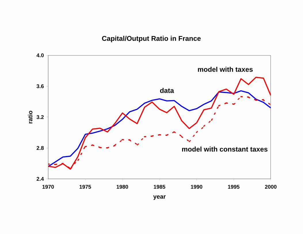
The base-case model does an impressive job in accounting for the evolution of GDP, hours
worked, and capital deepening in France. See Figures 11, 12 and 13, and Table 2.
Prescott (2002) argues that the tax wedge in labor supply is responsible for the difference in
hours worked between Europe and the US. Our results relative to the evolution over time
are consistent with it. This increases our confidence in the ability of our exercise to capture
the main aggregate performance of actual economies.
8. Sensitivity Analysis
In this section we evaluate how sensitive are our results to some of the key assumptions in
our exercise. We will explore separately the role of 4 key assumptions:

13
- The role of TFP growth, by comparing our results with a counterfactual in which TFP
would have grown at a constant rate.
- We recalibrate the preference parameters using data from the period 1975-2000 in order to
determine how sensitive are the results to our choice of the time period for the base-case
calibration.
- The intertemporal elasticity of substitution, by changing preferences to a CRRA
specification with higher than log curvature.
- The nature of government expenditure, by exploring the results under the assumption that
government consumption is wasted or used to finance the provision of public goods that
enter the utility function separably.
Table 3 summarizes the quantitative implications for all of our sensitivity analysis.
Constant TFP Growth
Consider the scenario in which TFP growth would have continued over the entire period
1970-2000 at the same average growth rate as it did during 1970-1974. This way we can
determine the contribution of the productivity slowdown for economic performance over
that period.
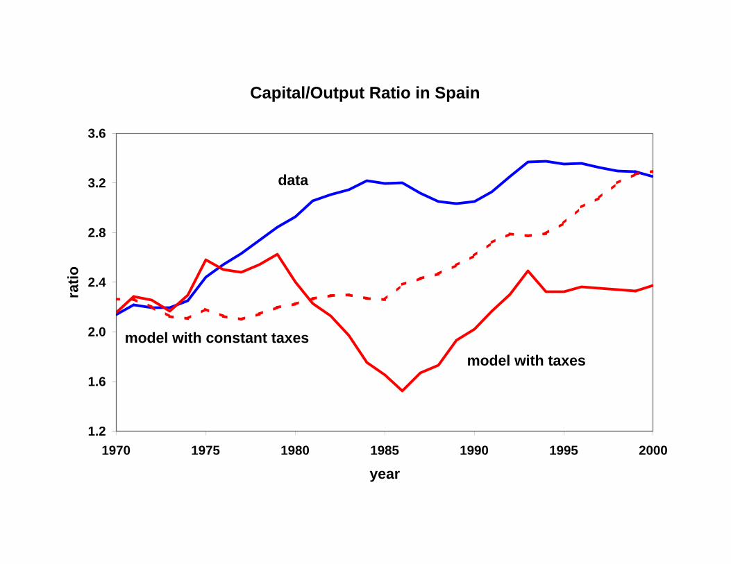
Our exercise shows that under this alternative scenario the model does equally well in
accounting for the evolution of aggregate hours worked, while it does worst in terms of the
evolution of the capital-output ratio and output per capita. From that we conclude that
productivity as measured in TFP did not have any impact in the evolution of hours worked.
Recalibrating Preference Parameters to 1975-2000
The key parameters are the preference parameters, and in order to determine those we used
data prior to 1975. The question now is to see to what extent our results are sensitive to that
choice.
In order to perform this sensitivity analysis we recalibrate the preference parameters using
data for the period 1975-2000 and we find values of 0.9917β = , 0.2904γ = .

14
Under this alternative parameterization hours worked are shifted downwards, so that the
model does better in accounting for the low level of hours worked after 1975, but then it is
inconsistent with the high levels observed prior to 1975. Also, the model does better in
terms of accounting for the evolution of the capital-output ratio.
Preferences Specification
In assuming log preferences we might be biasing our results in the sense that it implies an
intertemporal elasticity of substitution that some econometric studies focusing on individual
behaviour might find too high. In order to evaluate the implications of this feature for our
results we change the specification of preferences to:
1
1970 1 /t t t t
tt t
C N h LN N
φγ γ
β φ−
∞
=
⎛ ⎞⎡ ⎤⎛ ⎞ ⎛ ⎞−⎜ ⎟−⎢ ⎥⎜ ⎟ ⎜ ⎟⎜ ⎟⎢ ⎥⎝ ⎠ ⎝ ⎠⎣ ⎦⎝ ⎠∑
where tN is adult-equivalent population (we simply divide population by two) and 1φ = − .
In order to perform our sensitivity analysis we need to recalibrate the preference parameters
in our economy. We find values of 0.9918β = , 0.3365γ = .
Our results show that the model performs better in accounting for the evolution of hours
worked, but worse in accounting for capital accumulation.
Composition of Government Expenditure In our theoretical framework government revenues are lump-sum rebated to the consumers.
That implies that all tax revenues are either used to finance transfers or used to finance
consumption and investment goods that are perfect substitutes of consumer’s individual
choices. In this section we show how the results might change with respect to this
assumption.
In order to do so, we go to the other extreme and consider all of government consumption
in the National Accounts to be thrown into the ocean. Notice that this is clearly an extreme
15
scenario since a lot of government consumption finances goods that could otherwise be
provided by the private sector (health care, education,…).
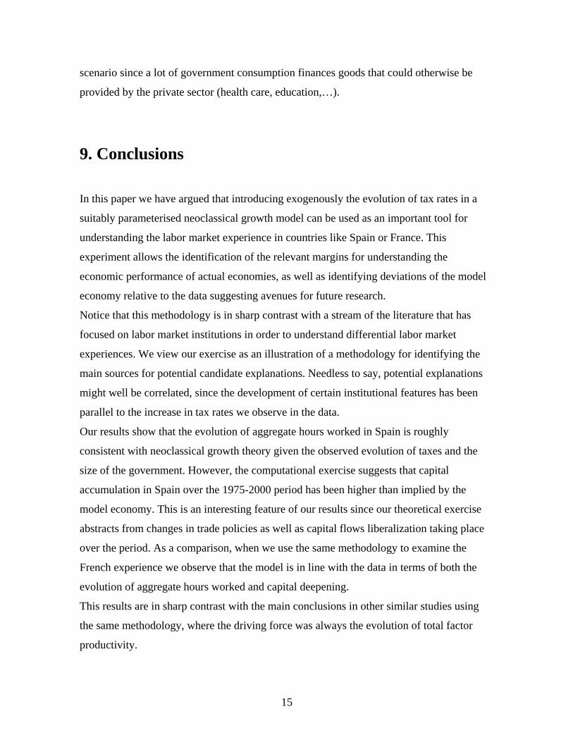
9. Conclusions
In this paper we have argued that introducing exogenously the evolution of tax rates in a
suitably parameterised neoclassical growth model can be used as an important tool for
understanding the labor market experience in countries like Spain or France. This
experiment allows the identification of the relevant margins for understanding the
economic performance of actual economies, as well as identifying deviations of the model
economy relative to the data suggesting avenues for future research.
Notice that this methodology is in sharp contrast with a stream of the literature that has
focused on labor market institutions in order to understand differential labor market
experiences. We view our exercise as an illustration of a methodology for identifying the
main sources for potential candidate explanations. Needless to say, potential explanations
might well be correlated, since the development of certain institutional features has been
parallel to the increase in tax rates we observe in the data.
Our results show that the evolution of aggregate hours worked in Spain is roughly
consistent with neoclassical growth theory given the observed evolution of taxes and the
size of the government. However, the computational exercise suggests that capital
accumulation in Spain over the 1975-2000 period has been higher than implied by the
model economy. This is an interesting feature of our results since our theoretical exercise
abstracts from changes in trade policies as well as capital flows liberalization taking place
over the period. As a comparison, when we use the same methodology to examine the
French experience we observe that the model is in line with the data in terms of both the
evolution of aggregate hours worked and capital deepening.
This results are in sharp contrast with the main conclusions in other similar studies using
the same methodology, where the driving force was always the evolution of total factor
productivity.

16
References
Bentolila, S. and G. Bertola (1990), “Firing Costs and Labor Demand: How Bad is Eurosclerosis?” Review of Economic Studies 57, 381-402. Blanchard, O. J. (2004), “The Economic Future of Europe,” NBER Working Paper 10310. Blanchard, O.J. and J. F. Jimeno (1995), “Structural Unemployment: Spain versus Portugal,” American Economic Review Papers and Proceedings 85, 212-218. Blanchard, O. J. and L. H. Summers (1986), “Hysteresis and the European Unemployment Problem,” NBER Macroeconomics Annual, 1. Cambridge, MA, MIT Press. Boscá, J. E., M. Fernández y D. Taguas (1999), “Estructura impositiva en los países de la OCDE,” Ministerio de Economía y Hacienda. Calonge, S. and J. C. Conesa (2003), “Progressivity and Effective Income Taxation in Spain: 1990 and 1995”, Universitat de Barcelona. Cole, H. L. and L. E. Ohanian (1999), “The Great Depression in the United States from a Neo-classical Perspective.” Federal Reserve Bank of Minneapolis Quarterly Review 23, 2-24. European Commission (2004), Statistical Annex, European Economy 6. Gollin, D. (2002), “Getting Income Shares Right,” Journal of Political Economy 110, 458-474. Gouveia, M. and R. P.Strauss (1994), “Effective federal individual income tax functions:An exploratory empirical analysis ”, National Tax Journal 47, 317-339. Hayashi, F. and E. C. Prescott (2002), “The 1990s in Japan: A Lost Decade,” Review of Economic Dynamics 5, 206-235. Jimenez-Martin, S. and A. Sanchez (2003), “An Evaluation of the Life-Cycle Effects of Minimum Pensions on Retirement Behavior”, UPF working paper 715. Kehoe, T. J. and E. C. Prescott (eds., 2002), “Great Depressions of the 20th Century,” Review of Economic Dynamics 5. Ljungqvist, L. and T. J. Sargent (1998), “The European Unemployment Dilemma,” Journal of Political Economy 106, 514-550. Ljungqvist, L. and T. J. Sargent (2002), “The European Employment Experience,” CEPR
17
Discussion Papers 3543. Marimón, R. and F. Zilibotti (1998), “Actual versus Virtual Employment in Europe: Is Spain Different?” European Economic Review 42, 123-153. Mendoza, E. G., A. Razin and L. L. Tesar (1994), “Effective Tax Rates in Macroeconomics. Cross-country Estimates of Tax Rates on Factor Incomes and Consumption,” Journal of Monetary Economics 34, 297-323. Nickell, S. (2003), “Employment and Taxes,” CESifo Working Paper Series No. 1109. Prescott, E. C. (2002), “Richard T. Ely Lecture: Prosperity and Depressions,” American Economic Review Papers and Proceedings, 92, 1-15. Prescott, E. C. (2004), “Why Do Americans Work So Much More than Europeans?” Federal Reserve Bank of Minneapolis Quarterly Review 28, 2-13. Sánchez, V. (2003), “Womens’ Employment and Fertility in Spain over the Last Twenty Years,” CAERP Working Paper 03/16.
18
Table 1
Growth Accounting in Spain
Decomposition of Average Annual Changes in Real GDP per Working-Age Person (Percent)
Data Model base case
Model constant taxes
1970-2000 Change in Y/N 2.18 2.01 3.40 Due to TFP 2.84 2.84 2.84 Due to K/Y 0.54 0.21 0.46 Due to L/N -1.20 -1.04 0.10 1970-1974 Change in Y/N 5.85 4.84 5.41 Due to TFP 5.47 5.47 5.47 Due to K/Y 0.47 -0.81 -1.02 Due to L/N -0.09 0.18 0.96 1974-1994 Change in Y/N 1.23 1.77 3.77 Due to TFP 3.07 3.07 3.07 Due to K/Y 0.81 0.25 0.50 Due to L/N -2.65 -1.54 0.20 1994-2000 Change in Y/N 2.90 0.92 0.81 Due to TFP 0.35 0.35 0.35 Due to K/Y -0.31 0.77 1.28 Due to L/N 2.87 -0.19 -0.82

19
Table 2
Growth Accounting in France
Decomposition of Average Annual Changes in Real GDP per Working-Age Person (Percent)
Data Model base case
Model constant taxes
1970-2000 Change in Y/N 1.90 1.60 2.77 Due to TFP 2.46 2.46 2.46 Due to K/Y 0.35 0.35 0.28 Due to L/N -0.91 -1.21 0.03

20
Table 3
Growth Accounting in Spain: Sensitivity Analysis
Decomposition of Average Annual Changes in Real GDP per Working-Age Person (Percent)
Data
Model base case
Model constant
TFP growth
Model recalibrated parameters
Model alternative
utility
Model government consumption
Model myopic
expectations1970-2000 Change in Y/N 2.18 2.01 2.71 2.11 2.30 2.20 1.94 Due to TFP 2.84 2.84 4.24 2.84 2.84 2.84 2.84 Due to K/Y 0.54 0.21 -0.23 0.50 0.59 0.24 0.32 Due to L/N -1.20 -1.04 -1.30 -1.23 -1.13 -0.88 -1.221970-1974 Change in Y/N 5.85 4.84 3.75 5.39 5.46 5.31 5.13 Due to TFP 5.47 5.47 4.24 5.47 5.47 5.47 5.47 Due to K/Y 0.47 -0.81 0.35 -0.04 0.16 -0.56 -0.36 Due to L/N -0.09 0.18 -0.84 -0.04 -0.17 0.40 0.021974-1994 Change in Y/N 1.23 1.77 2.11 1.77 2.01 1.90 1.65 Due to TFP 3.07 3.07 4.24 3.07 3.07 3.07 3.07 Due to K/Y 0.81 0.25 -0.17 0.57 0.63 0.33 0.40 Due to L/N -2.65 -1.54 -1.96 -1.87 -1.69 -1.50 -1.821994-2000 Change in Y/N 2.90 0.92 4.00 1.16 0.25 1.12 0.79 Due to TFP 0.35 0.35 4.24 0.35 0.35 0.35 0.35 Due to K/Y -0.31 0.77 -0.83 0.73 0.58 0.47 0.49 Due to L/N 2.87 -0.19 0.59 0.08 -0.68 0.30 -0.04
Growth Accounting for Spain 1960-2000
50
100
150
200
250
300
350
400
1960 1965 1970 1975 1980 1985 1990 1995 2000
year
inde
x (1
960=
100)
11tA α−
/t tL N
/t tY N
( )1/t tK Yαα−

Work in Spain 1960-2000
50
60
70
80
90
100
110
1960 1965 1970 1975 1980 1985 1990 1995 2000year
1960
=100
hours per working age person
employment rate
hours per worker

Hours Worked per Working-Age Person
14
16
18
20
22
24
26
28
1960 1965 1970 1975 1980 1985 1990 1995 2000
year
hour
s pe
r wee
k
United States
France
Spain
Growth Accounting for France 1960-2000
50
100
150
200
250
300
350
400
1960 1965 1970 1975 1980 1985 1990 1995 2000
year
inde
x (1
960=
100)
11tA α−
/t tY N
( )1/t tK Yαα−
/t tL N
Marginal Tax Rates in Spain
0.00
0.10
0.20
0.30
0.40
0.50
1965 1970 1975 1980 1985 1990 1995 2000
year
perc
ent
taxes on labor
taxes on consumption
taxes on capital

Detrended Real GDP per Working-Age Person in Spain
70
80
90
100
110
120
130
1970 1975 1980 1985 1990 1995 2000
year
inde
x (1
975=
100)
data
model with constant taxes
model with taxes
Hours Worked per Working-Age Person in Spain
14
16
18
20
22
24
26
28
1970 1975 1980 1985 1990 1995 2000
year
hour
s pe
r wee
k
data
model with taxes
model with constant taxes
Capital/Output Ratio in Spain
2.0
2.4
2.8
3.2
3.6
1970 1975 1980 1985 1990 1995 2000
year
ratio
data
model with constant taxes
model with taxes

Marginal Tax Rates in France
0.00
0.10
0.20
0.30
0.40
0.50
0.60
1970 1975 1980 1985 1990 1995 2000
year
perc
ent
taxes on labor
taxes on consumption
taxes on capital

Real GDP per Working-Age Person in France
80
90
100
110
120
130
1970 1975 1980 1985 1990 1995 2000
year
inde
x (1
970=
100)
data
model with constant taxes
model with taxes

Hours Worked per Working-Age Person in France
14
16
18
20
22
24
26
28
1970 1975 1980 1985 1990 1995 2000
year
hour
s pe
r wee
k
data
model with taxes
model with constant taxes
Capital/Output Ratio in France
2.4
2.8
3.2
3.6
4.0
1970 1975 1980 1985 1990 1995 2000
year
ratio
data
model with constant taxes
model with taxes

Detrended Real GDP per Working Age Person in Spain
60
70
80
90
100
110
120
130
140
1970 1975 1980 1985 1990 1995 2000
year
inde
x (1
975=
100)
data
model with constant taxes
model with taxes
Hours Worked per Working Age Person in Spain
14
16
18
20
22
24
26
28
1970 1975 1980 1985 1990 1995 2000
year
hour
s pe
r wee
k
data
model with taxes
model with constant taxes
Capital/Output Ratio in Spain
1.2
1.6
2.0
2.4
2.8
3.2
3.6
1970 1975 1980 1985 1990 1995 2000
year
ratio
data
model with constant taxesmodel with taxes
Top Related