


Languages
Pages
Legal


Problem Definitions and Evaluation
Criteria for CEC 2011 Competition on
Testing Evolutionary Algorithms on Real
World Optimization Problems
Swagatam Das1 and P. N. Suganthan2
1Dept. of Electronics and Telecommunication Engg. , Jadavpur University, Kolkata 700 032, India
2School of Electrical and Electronic Engineering,
Nanyang Technological University, Singapore 639798, Singapore
E-mails: [email protected], [email protected]
Technical Report, December, 2010

2
We thankfully acknowledge the contribution of the following friends, colleagues and
students in making the problem set complete:
1. Dr. B. K. Panigrahi, Indian Institute of Technology (IIT) Delhi, India.
2. Dr. Chit Hong Yam, European Space Agency, Advanced Concepts Team
(http://www.esa.int/act), ESTEC, DG-PF, Keplerlaan 1 – 2201, AZ Noordwijk
- The Netherlands.
3. Dr. P. K. Rout, ITER, SOA University, Orissa, India.
4. Mr. Krishnanand K. R, Multi-disciplinary Research Cell, SOA University,
Orissa, India.
5. Mr. Siddharth Pal, Dept. of Electronics and Telecommunications Engineering,
Jadavpur University, India.
6. Mr. Aniruddha Basak, Dept. of Electronics and Telecommunications
Engineering, Jadavpur University, India.
7. Mr. Sayan Maity, Dept. of Electronics and Telecommunications Engineering,
Jadavpur University, India.
We express our deep gratitude to Prof. Lin-Yu Tseng and Mr. Chun Chen of
National Chung Hsing University, Taichung, Taiwan, for their huge efforts in
translating the MATLAB source code package to C programming language. We
also thank Dr Antonio LaTorre from CeSViMa - Universidad Politécnica de
Madrid for generating a Linux C package.

3
A comprehensive account of some real world optimization problems have been presented in
details. These problems can be used to evaluate the performance of different stochastic
optimization algorithm. After all, every optimization algorithm has to be applied to some real
world problems. In light of this fact, some real world optimizations problems have been
selected and detailed analysis of those problems have given to understand it and the objective
functions have been evaluated respected to the constraints (if any) to optimize and get its
solution.
1. Problem Definitions
In this section some real world problems to evaluate the performance of algorithms are defined.
1. Parameter Estimation for Frequency-Modulated (FM) Sound Waves (Problem No.1
in Table 1)
Frequency-Modulated (FM) sound wave synthesis has an important role in several modern
music systems and to optimize the parameter of an FM synthesizer is a six dimensional
optimization problem where the vector to be optimized is 1 1 2 2 3 3, , , , ,X a a aω ω ω= of the
sound wave given in eqn. (1). The problem is to generate a sound (1) similar to target sound
(2). This problem is a highly complex multimodal one having strong epistasis, with minimum
value ( ) 0solf X =r
. This problem has been tackled using Genetic Algorithms (GAs) in [1],
[2].The expressions for the estimated sound and the target sound waves are given as:
( )( )( )1 1 2 2 3 3( ) .sin . . .sin . . .sin . .y t a t a t a tω θ ω θ ω θ= + + (1)
( ) ( ) ( ) ( ) ( )( )( )( )0 ( ) (1.0).sin 5.0 . . 1.5 .sin 4.8 . . 2.0 .sin 4.9 . .y t t t tθ θ θ= − + (2)
respectively where 2 100θ π= and the parameters are defined in the range [ ]6.4 6.35−
The fitness function is the summation of square errors between the estimated wave (1) and
the target wave (2) as follows:

4
( )100 2
00( ) ( ) ( )
tf X y t y t
== −∑
r (3)
2. Lennard-Jones Potential Problem (Problem No. 2 in Table 1)
It is a potential energy minimization problem. Lennard-jones potential problem involves the
minimization of molecular potential energy associated with pure Lennard-Jones (LJ) cluster
[3], [4]. This is a multi-modal optimization problem comprised of an exponential number of
local minima [3]. The lattice structure of LJ cluster has an icosahedral core and a combination
of surface lattice points. Most of the global minima have structures based upon the Mackay
icosahedrons an can be seen in the Cambridge Cluster Database (http://www-
wales.ch.cam.ac.uk/CCD.html). An algorithm can be tasted over this function for its
capability to conform molecular structure, where the atoms are organized in such a way that
the molecule has minimum energy. Lennard-Jones pair potential for N atoms, given by the
Cartesian coordinates
, , , 1,...,i i i ip x y z i N= =r r r r
(4)
is given as follows:
( ) ( )1
12 6
1 1V 2. ,
N N
N ij iji j i
p r r−
− −
= = +
= −∑ ∑ (5)
where 2ij j ir p p= −
r rwith gradient
( ) ( )( )14 8
1,12 , 1,...,
N
j N ij ij j ii i j
V p r r p p j N− −
= ≠
∇ =− − − =∑ r r (6)
Lennard-Jones potential has minimum value at a particular distance between the two points
[5]. The structures of LJ clusters after optimization take following shapes as reported by
Cambridge Cluster Database.

5
N = N=
(a) (b) N = N = (c) (d)
Fig. 1: (a), (b), (c), and (d) are the shapes for 38, 75, 102 and 104 atom LJ clusters and the
optimum potential reported up to now are -173.928427, -402.894866, -569.363652 and -
582.086642 respectively pair well depth.
The variation of Lennard-Jones pair potential V(r) = r-12-2.r-6 with pair distance r have
been plotted in Figure 2. It can be clearly seen that it has a unique minimum value of -1 for a
particular value of r (=1). Its value increases very fast when r is decreased from the
optimum value and tends to infinity near r=0. This tendency of pair potential curve makes it
a hard optimization problem.

6
0 1 2 3 4 5 6-1
0
1
2
3
4
5
6
7
r
V(r)
Fig. 2: Variation of pair potential with r
Following [4], we can reduce the dimension of the problem in the following way. We first fix
an atom at the origin and choose our second atom to lie on the positive X-axis. The third atom
can then be selected to lie in the upper half of the X-axis. Since the position of the first atom
is always fixed and the second atom is restricted to the positive X-axis, this gives a
minimization problem involving three variables for three atoms. For four atoms, additionally
three variables (the Cartesian co-ordinates of the 4-th atom) are required to give a
minimization problem in six independent variables. For each further atom, three variables
(coordinates of the position of the atom) are added to determine the potential energy of
clusters. Let xr be the variable of the problem which has three components for three atoms, six
components for 4 atoms and so on. The first variable due to the second atom i.e. 1 [0, 4]x ∈ ,
then the second and third variables are such that 2 [0, 4]x ∈ and 3 [0, ]x π∈ . The coordinates
ix for any other atom is taken to be bound in the range:
1 4 1 44 ,44 3 4 3
i i⎡ ⎤− −⎢ ⎥ ⎢ ⎥− − +⎢ ⎥⎢ ⎥ ⎢ ⎥⎣ ⎦ ⎣ ⎦⎣ ⎦
where r⎢ ⎥⎣ ⎦ is the nearest least integer w.r.t. r∈ .
7
3. The Bifunctional Catalyst Blend Optimal Control Problem (Problem No. 3 in
Table 1)
Luus [6, 7] studied a hard multimodal optimal control problem which has many local optima.
As many as 300 local optima have been reported by Esposito and Floudas [8]. The proposed
problem is a chemical process which converts methylcyclopentane to benzene in a tubular
reactor and described by a set of following seven differential equations:
1 1 1,x k x= −& (4)
( )2 1 1 2 3 2 4 5 ,x k x k k x k x= − + +& (8)
3 2 2 ,x k x=& (9)
4 6 4 5 5 ,x k x k x= − +& (10)
( )5 3 2 6 4 4 5 8 9 5 7 6 10 7 ,x k x k x k k k k x k x k x= − + − + + + + +& (11)
6 8 5 7 6 ,x k x k x= −& (12)
7 9 5 10 7x k x k x= −& (13)
where , 1,2,...,7ix i = are the mole fractions of the chemical species, and the rate constants
( )ik are cubic functions of the catalyst blend ( )u t :
2 3
1 2 3 4 , 1, 2,...,10i i i i ik c c u c u c u i= + + + = (14)
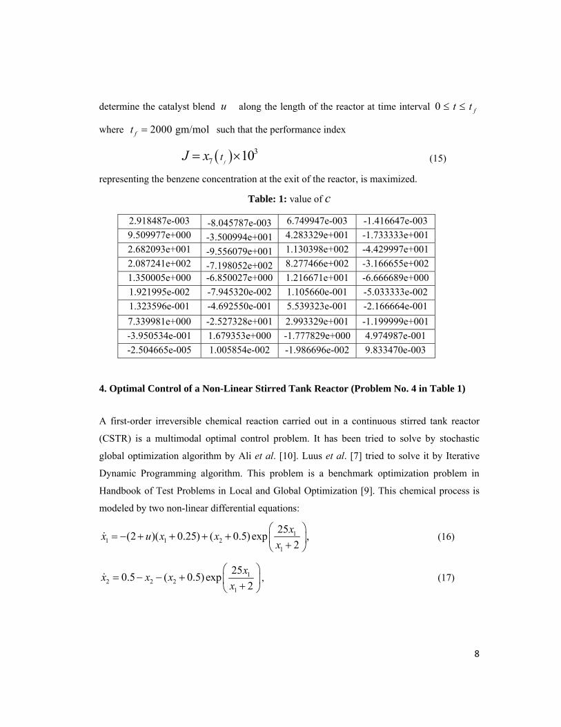
Where the values of the coefficients cij are experimentally evaluated are given in Table 1[7].
The mass fraction of the hydrogenation catalyst is bounded as: 0.6 ( ) 0.9u t≤ ≤ and
initially [ ][0] 1 0 0 0 0 0 0 Tx = . This chemical process is operated in steady state
and hence 1x appears at the beginning of the process and 7x at the end, so 1x through
7x can be considered to be placed along the length of the tubular reactor. The objective is to
8
determine the catalyst blend u along the length of the reactor at time interval 0 ft t≤ ≤
where 2000 gm/molft = such that the performance index
( ) 37 10
ftJ x= × (15)
representing the benzene concentration at the exit of the reactor, is maximized.
Table: 1: value of c
2.918487e-003 -8.045787e-003 6.749947e-003 -1.416647e-003 9.509977e+000 -3.500994e+001 4.283329e+001 -1.733333e+001 2.682093e+001 -9.556079e+001 1.130398e+002 -4.429997e+001 2.087241e+002 -7.198052e+002 8.277466e+002 -3.166655e+002 1.350005e+000 -6.850027e+000 1.216671e+001 -6.666689e+000 1.921995e-002 -7.945320e-002 1.105660e-001 -5.033333e-002 1.323596e-001 -4.692550e-001 5.539323e-001 -2.166664e-001 7.339981e+000 -2.527328e+001 2.993329e+001 -1.199999e+001 -3.950534e-001 1.679353e+000 -1.777829e+000 4.974987e-001 -2.504665e-005 1.005854e-002 -1.986696e-002 9.833470e-003
4. Optimal Control of a Non-Linear Stirred Tank Reactor (Problem No. 4 in Table 1)
A first-order irreversible chemical reaction carried out in a continuous stirred tank reactor
(CSTR) is a multimodal optimal control problem. It has been tried to solve by stochastic
global optimization algorithm by Ali et al. [10]. Luus et al. [7] tried to solve it by Iterative
Dynamic Programming algorithm. This problem is a benchmark optimization problem in
Handbook of Test Problems in Local and Global Optimization [9]. This chemical process is
modeled by two non-linear differential equations:
11 1 2
1
25(2 )( 0.25) ( 0.5)exp ,2
xx u x xx
⎛ ⎞= − + + + + ⎜ ⎟+⎝ ⎠
& (16)
12 2 2
1
250.5 ( 0.5)exp2
xx x xx
⎛ ⎞= − − + ⎜ ⎟+⎝ ⎠
& , (17)

9
( )u t = Flow rate of the cooling fluid, 1x = Dimensionless steady state temperature and
2x = Deviation from dimensionless steady state concentration. The optimization objective is
to determine suitable value of u so that the performance index
0.72 2 2 21 20
( 0.1. ) ,ftJ x x u dt
== + +∫ (18)
is minimizes where the initial conditions are ( ) [ ]0 0.0.9 0.09 Tx = . Though the problem is
unconstrained the initial guess for ( )u t lies in [ ]0.0 5.0 . The integration involved in
evaluation is performed using sub-function ode45 available in MATLAB with relative
tolerance set to 11 10−× .
5. Tersoff Potential Function Minimization Problem (Problem No. 5 & 6 in Table 1)
Evaluation of inter atomic potentials for covalent systems, particularly for Silicon has been
receiving great interest from the researchers. One such potential is Tersoff potential, which
governs the interaction of silicon atoms with a strong covalent bonding. Tersoff has given
two parameterization of silicon and these are called Sc(B) and Sc(C). If we define the
positions of the molecular clusters of N atoms by:
1 2 , , ..., ,NX X X X=r r r r
(19)
where iXr
s 1, 2,...,i N∈ is a three-dimensional vector denoting the coordinates of the ith
atom in Cartesian coordinate system then the total Tersoff potential energy function of the
system is a function of atomic co-ordinates and defined as
1 3 1 1 3 1 3( ,..., ) ( ,..., ) ... ( ,..., )Nf X X E X X E X X= + +r r r r r r
(20)
Total potential is sum of individual potentials of atoms given by eqn. (21), which further
needs calculation of eqn. (22) through (27). The potential of any atom depends on the
physical position of their neighbor atoms. Different atoms have different distances and angles

10
subtended with respect to the other atoms so every atom has deferent energies. Now the
Tersoff potential [11] of individual atoms can be formally defined as
( ) ( ) ( )( )1 ,
2i c ij R ij ij R ijj iE f r V r B V r i
≠= − ∀∑ (21)
where ijr is the distance between atoms i and j, VR is a repulsive term, VA is an attractive
term, ( )c ijf r is a switching function and Bij is a many-body term that depends on the
positions of atoms i and j and the neighbors of atom i. These quantities are detailed in [11].
1
11
1 21
nnnBij ijγ ξ⎛ ⎞⎜ ⎟⎝ ⎠
−= + (22)
where ni and γ are known fitted parameters [11] . The term ξij for atoms i and j (i.e., for
bond ij ) is given by:
( ) ( ) ( )( )333expij c ij ijk ij ik
k if r g r rξ θ λ
≠
= −∑ (23)
Here ξij describes the contribution of the neighbors of the atom , ξij increases as the number
of k atoms increases but the term Bij decreases as ξij increases. The exponential term in (23) is
designed to reduce the contribution of bonds with length greater than ijr , so that the distant
neighbors of have a reduced contribution to the bond order term. The term ijkθ is the bond
angle between bonds ij and ik, and the function g is given by:
( ) ( )( )( )22 2 2 21 cosijk ijkg c d c d hθ θ= + − + − (24)
The parameter h is the cosine of the optimum bond angle and c and d control the
influence of bond angles on the many-body term. The quantities 3, , and c d hλ which appear

11
in (23) and (24) are also known fitted parameters. The terms ( )R ijV r and ( )A ijV r are given
by:
( ) 1 ijrR ijV r Ae λ−=
(25)
( ) 2 ijrA ijV r Be λ−=
(26)
where A,B, 1λ and 2λ are given fitted parameters. The switching function ( )c ijf r restricts
the potential calculations to nearest neighbors only and ensures that atomic interactions decay
smoothly to zero as the separation distance increases. It is given by
( ) ( )1, if 1 1 sin / , if 2 20, if
ij
c ij ij ij
ij
r R D
f r r R D R D r R D
r R D
π
≤ −
⎡ ⎤= − − − ⟨ ⟨ +⎣ ⎦
≥ +
⎧⎪⎪⎨⎪⎪⎩
(27)
The two sets of parameter values respectively for Si(B) and Si(C) is tabulated in Table 2 [12].
Though Tersoff potential problem is a 3N × dimensional in 3-dimentional space, the no. of
dimensions to be evaluated can be decreased in light of the fact that it depends on relative
position of atom instead of actual Cartesian coordinates. One atom can be permanently put on
the origin and second atom on the positive x-axis. Thus for a 3-atom system the actual no. of
variables is four instead of nine. Now, for each additional atom added to the system, the no.
of variables increases by three (three Cartesian coordinates of an additional atom). Thus, in
general, for the system of N atoms, the no. of unknown variables is 3 6n N= × − . Now the
cluster X of N atoms can be redefined as
( )3 61 2, ,..., , N
nx x x x x IR −= ∈ (28)
The search region for both Si (B) and Si(C) model of Tersoff potential is
1 2 1 2 3, ,..., | 4.25 , 4.25, 4,..., 0 4,0n ix x x x x i n x x πΩ = − ≤ ≤ = ≤ ≤ ≤ ≤
(29)
12
The potential (29) is a complex and differentiable function whose partial derivatives can be
found in [11]. The cost function now can be redefined as:
( ) ( ) ( ) ( )1 2 ... , Nf x E x E x E x x= + + + ∈Ω (30)
Note that in this case also the variables are initialized in the same way as was done for the
Lennard-Jones potential minimization problem.
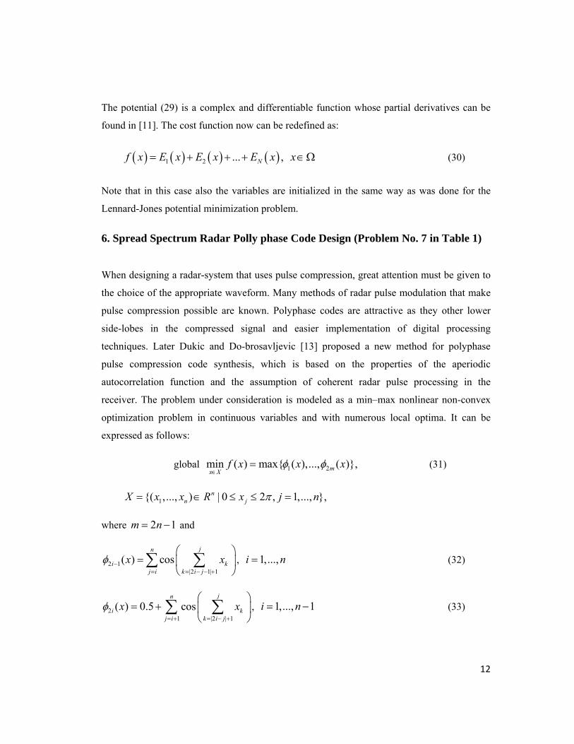
6. Spread Spectrum Radar Polly phase Code Design (Problem No. 7 in Table 1)
When designing a radar-system that uses pulse compression, great attention must be given to
the choice of the appropriate waveform. Many methods of radar pulse modulation that make
pulse compression possible are known. Polyphase codes are attractive as they other lower
side-lobes in the compressed signal and easier implementation of digital processing
techniques. Later Dukic and Do-brosavljevic [13] proposed a new method for polyphase
pulse compression code synthesis, which is based on the properties of the aperiodic
autocorrelation function and the assumption of coherent radar pulse processing in the
receiver. The problem under consideration is modeled as a min–max nonlinear non-convex
optimization problem in continuous variables and with numerous local optima. It can be
expressed as follows:
global 1 2min ( ) max ( ),..., ( ),mx Xf x x xφ φ
∈= (31)
1( ,..., ) | 0 2 , 1,..., ,nn jX x x R x j nπ= ∈ ≤ ≤ =
where 2 1m n= − and
2 1|2 1| 1
( ) cosjn
i kj i k i j
x xφ −= = − − +
⎛ ⎞= ⎜ ⎟
⎝ ⎠∑ ∑ , 1,...,i n= (32)
21 |2 | 1
( ) 0.5 cosjn
i kj i k i j
x xφ= + = − +
⎛ ⎞= + ⎜ ⎟
⎝ ⎠∑ ∑ , 1,..., 1i n= − (33)
13
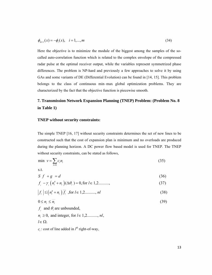
( ) ( ), 1,...,m i ix x i mφ φ+ = − = (34)
Here the objective is to minimize the module of the biggest among the samples of the so-
called auto-correlation function which is related to the complex envelope of the compressed
radar pulse at the optimal receiver output, while the variables represent symmetrized phase
differences. The problem is NP-hard and previously a few approaches to solve it by using
GAs and some variants of DE (Differential Evolution) can be found in [14, 15]. This problem
belongs to the class of continuous min–max global optimization problems. They are
characterized by the fact that the objective function is piecewise smooth.
7. Transmission Network Expansion Planning (TNEP) Problem: (Problem No. 8
in Table 1)
TNEP without security constraints:
The simple TNEP [16, 17] without security constraints determines the set of new lines to be
constructed such that the cost of expansion plan is minimum and no overloads are produced
during the planning horizon. A DC power flow based model is used for TNEP. The TNEP
without security constraints, can be stated as follows,
min (35)
s.t.
l ll
v c n
S f g d
∈Ω
=
+ =
∑
( )( )
0
___0
(36)
( ) 0, for 1,2.........., (37)
,for 1,2..........,
l l l l l
l l l l
f n n l
f n n f l nl
γ θ− + Δ = ∈
≤ + ∈___
(38)
0 (39) and are unbounded,
0, and integer, for 1,2.........., ,.
l
l l
l
l
n nf
n l nll
θ≤ ≤
≥ ∈
∈Ω
lc : cost of line added in lth right-of-way,

14
S : branch-node incidence transposed matrix of the power system,
f :vector with elements l
f ,
lγ : susceptance of the circuit that can be added to lth right-of-way,
ln : the number of circuits added in lth right-of-way,
0ln : no. of circuits in the base case,
lθΔ : phase angle difference in lth right-of way,
lf : total real power flow by the circuit in lth right-of-way ,
___
lf : maximum allowed real power flow in the circuit in lth right-of-way,
___
ln :maximum number of circuits that can be added in lth right-of-way,
Ω :set of all right-of-ways,
nl: total number of lines in the circuit.
The objective is to minimize the total investment cost of the new transmission lines to be
constructed, satisfying the constraint on real power flow in the lines of the network.
Constraint (38) represents the power balance at each node. Constraint (37) is the real power
flow equations in DC network. Constraint (38) represents the line real power flow constraint.
Constraint (39) represents the restriction on the construction of lines per corridor (R.O.W).
The transmission lines added in any right-of–way are the decision variables.
The cost of each solution to the TNEP without security constraints can be obtained using the
eqn.(40) as shown below:
Minimize:
___
1 2W (abs ( ) ) +W ( - ) ll l l l ll ol
f c n f f n n∈Ω
= + −∑ ∑ (40)
ol: represents the set of overloaded lines.
The objective of the TNEP is to find the set of transmission lines to be constructed such that
the cost of expansion plan is minimum and no overloads are produced during the planning

15
horizon. Hence, first term in the equation (40) indicates the total investment cost of a
transmission expansion plan. The second term is added to the objective function for the real
power flow constraint violations. The third term is added to the objective function if
maximum number of circuits that can be added in lth right-of-way exceeds the maximum
limit. W1, W2 are constants. The second and third terms are added to the fitness function only
in case of violations.
8. Large Scale Transmission Pricing Problem (Problem No. 9 in Table 1)
In the modern era of deregulated power systems, transmission pricing is one of the
extensively debated issues in literature [18-20]. The unbundling of vertically integrated
utilities creates transmission owner as a separate identity. The transmission pricing, as per
generic perception, tackles the issue of allocating the fixed costs of transmission to various
stake-holders. Many factors influence the decision about the scheme of transmission pricing
to be adopted. Some of the factors could be: ex-ante / ex-post pricing, market based / non-
market methods, methods for centralized or decentralized markets, whether loss is part of
transmission pricing or not, etc. The list is quite exhaustive and hence is the number of
proposed methods of transmission pricing.
Equivalent Bilateral Exchange (EBE) is one such method introduced in [19] that works on the
linearized model of the system. The original scheme is developed for a pool market (non-
transaction based), in order to calculate the final transmission charges for each node. The
method imposes a rule on the established power flow snap-shot. The rule is based on the
assumption that every generator contributes to every load. The amount of contribution is
decided in proportionate manner. The method provides fair price signals and proves to be
useful in pool system, where, bilateral transactions are non-existent.
The original EBE method [19] creates a load-generation interaction matrix (equivalent
bilateral exchange) based on the following proportionality principle:
16
sysD
DjGiij P
PPGD = , (41)
where, GDij is the amount of equivalent bilateral exchange that takes place between
generator i and load j and sysDP is the total load in the system. Now the fraction of power flow
in line k due to bilateral exchange between generation at bus i and demand at bus j is
evaluated for all equivalent bilateral power exchanges using DC load flow or by using PTDF
[18]. The net flow in the line k is the absolute sum of all the flows due to all the transactions.
The net flow in the line can be expressed in terms of equivalent bilateral power exchanges as
∑∑=i j
ijkijk GDpf γ (42)
Equation (43) shows that creating an equivalent bilateral transaction matrix using
proportionality principle is not the only way to do the pricing. There are multiple solutions
possible. Though proportionate principle is logical or intuitive way of decomposing, it needs
to be seen how the multiplicity of solutions can be used for proper applications.
Problem Statement
If there are pre-existing bilateral transactions, it creates a division amongst the existing
customers: Bilateral customers and pool customers. Hence, we suggest a different
transmission pricing schemes for these two sets of customers. Since the bilateral transactions
are a-priori known, the usage rate for the BT are calculated using PTDF and evaluating usage
of lines by BTs. Thus, in step 1, some of the total charges to be recovered are attributed to
BTs. The rest of the charges are now recovered through pool customers. However, the
allocation of these remaining charges and calculation of rates thereby, is done using
optimization. As mentioned earlier, the optimization helps in exploring the multiple solutions
in deciding the equivalent bilateral exchanges such that the charges of pool customers are
close to those had BTs been absent. The formulation is discussed next.

17
Problem Formulation
An input file, containing the bus specifications, line specifications, fixed cost to be recovered
and bilateral transactions data, is considered as the problem definition. The sensitivity of a
line connecting bus m and n for a transaction between buses i and j are given by [18] as
, ,mi ni mj njij mn
mn
X X X Xx
γ− − −
= (43)
where mnx is the reactance of line connecting buses m and n; miX , niX , mjX and njX entries
of the X matrix[18].
Usage rates with pool only market:
The EBE method [19] is applied on the given data and the transmission charges in
Rs/Mwhr are evaluated at each bus. Let igeR is the obtained transmission usage rate for a
generation at bus i and jdeR be the obtained transmission usage rate for a demand at bus j.
Usage rates with pool and bilateral transactions:
i) The equivalent bilateral transactions between pool generations and pool demands are
obtained by minimizing usage rate deviations due to bilateral transactions i.e.
minijGD ( )ijF GD =
2
'
. .
kk
ij ijj k k k
ij ij ij iji j i j
ige
gi gii
FCGD
GD BT
RP P
γ
γ γ
⎡ ⎤⎡ ⎤⎡ ⎤⎡ ⎤⎢ ⎥⎢ ⎥⎢ ⎥⎢ ⎥⎢ ⎥⎢ ⎥⎢ ⎥⎢ ⎥⎢ ⎥⎢ ⎥⎢ ⎥⎢ ⎥⎢ ⎥⎢ ⎥⎢ ⎥⎢ ⎥⎡ ⎤⎢ ⎥⎢ ⎥⎢ ⎥⎢ ⎥⎢ ⎥+⎢ ⎥⎢ ⎥⎢ ⎥⎢ ⎥⎢ ⎥⎢ ⎥⎢ ⎥⎢ ⎥⎢ ⎥⎣ ⎦⎣ ⎦⎣ ⎦⎢ ⎥⎣ ⎦ −⎢ ⎥−⎢ ⎥⎢ ⎥⎢ ⎥⎢ ⎥⎢ ⎥⎢ ⎥⎢ ⎥⎢ ⎥⎣ ⎦
∑ ∑∑∑ ∑∑
∑ +
18
'
. .
kk
ij iji k k k
ij ij ij iji j i j
jde
dj djj
FCGD
GD BT
RP P
γ
γ γ
⎡ ⎤⎡ ⎤⎡ ⎤⎡ ⎤⎢ ⎥⎢ ⎥⎢ ⎥⎢ ⎥⎢ ⎥⎢ ⎥⎢ ⎥⎢ ⎥⎢ ⎥⎢ ⎥⎢ ⎥⎢ ⎥⎢ ⎥⎢ ⎥⎢ ⎥⎢ ⎥⎡ ⎤⎢ ⎥⎢ ⎥⎢ ⎥⎢ ⎥⎢ ⎥+⎢ ⎥⎢ ⎥⎢ ⎥⎢ ⎥⎢ ⎥⎢ ⎥⎢ ⎥⎢ ⎥⎢ ⎥⎣ ⎦⎣ ⎦⎣ ⎦⎢ ⎥⎣ ⎦+ −⎢ ⎥−⎢ ⎥⎢ ⎥⎢ ⎥⎢ ⎥⎢ ⎥⎢ ⎥⎢ ⎥⎢ ⎥⎣ ⎦
∑ ∑∑∑ ∑∑
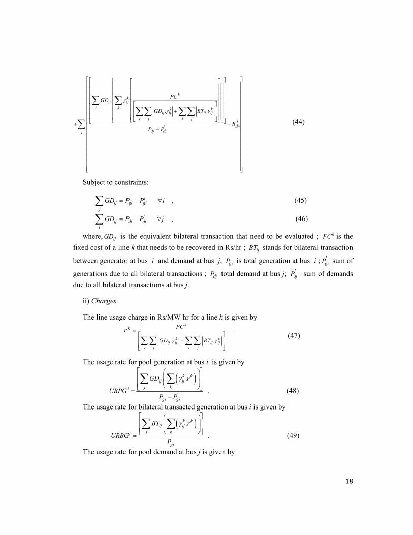
∑ (44)
Subject to constraints: i
ij gi gij
GD P P= −∑ i∀ , (45)
'ij dj dj
i
GD P P= −∑ j∀ , (46)
where, ijGD is the equivalent bilateral transaction that need to be evaluated ; kFC is the fixed cost of a line k that needs to be recovered in Rs/hr ; ijBT stands for bilateral transaction
between generator at bus i and demand at bus j; giP is total generation at bus i ; 'giP sum of
generations due to all bilateral transactions ; djP total demand at bus j; 'djP sum of demands
due to all bilateral transactions at bus j. ii) Charges The line usage charge in Rs/MW hr for a line k is given by
.
. .
k
k kij ij ij ij
i j i j
k FC
GD BT
rγ γ
=⎡ ⎤⎢ ⎥+⎢ ⎥⎣ ⎦∑∑ ∑∑
(47)
The usage rate for pool generation at bus i is given by
( )'
.
.
k kij ij
j ki
gi gi
GD r
URPGP P
γ⎡ ⎤⎛ ⎞⎢ ⎥⎜ ⎟⎜ ⎟⎢ ⎥⎝ ⎠⎣ ⎦=
−
∑ ∑ (48)
The usage rate for bilateral transacted generation at bus i is given by
( )
'
.
.
k kij ij
j ki
gi
BT r
URBGP
γ⎡ ⎤⎛ ⎞⎢ ⎥⎜ ⎟⎜ ⎟⎢ ⎥⎝ ⎠⎣ ⎦=∑ ∑
(49)
The usage rate for pool demand at bus j is given by
19
( )'
.
.
k kij ij
i kj
dj dj
GD r
URPDP P
γ⎡ ⎤⎛ ⎞⎢ ⎥⎜ ⎟⎜ ⎟⎢ ⎥⎝ ⎠⎣ ⎦=
−
∑ ∑ (50)
The usage rate for bilateral transacted demand at bus j is given by,
dj
j k
kkijij
j
P
rBTURBD
∑ ∑ ⎟⎟⎠
⎞⎜⎜⎝
⎛
=
γ (51)
The present instantiation of the problem is on IEEE 30 bus system. We have assumed that the
fixed cost to be recovered is US$ 100/hr and the cost of each element is proportional to the
line reactance as the element costs are unavailable for this network system. First, a base case
DC load flow is run and the charges for each bus using original EBE scheme are calculated.
Then, we superimpose additional bilateral transactions over the base case data to realize a
combined pool and bilateral market. The charges for BTs and Pool customers can be
calculated using equations (48 - 51). The charges for generators and loads in Pool scheme are
calculated using equation (48) and (50) respectively, such that the objective function of
equation (44) is minimized.
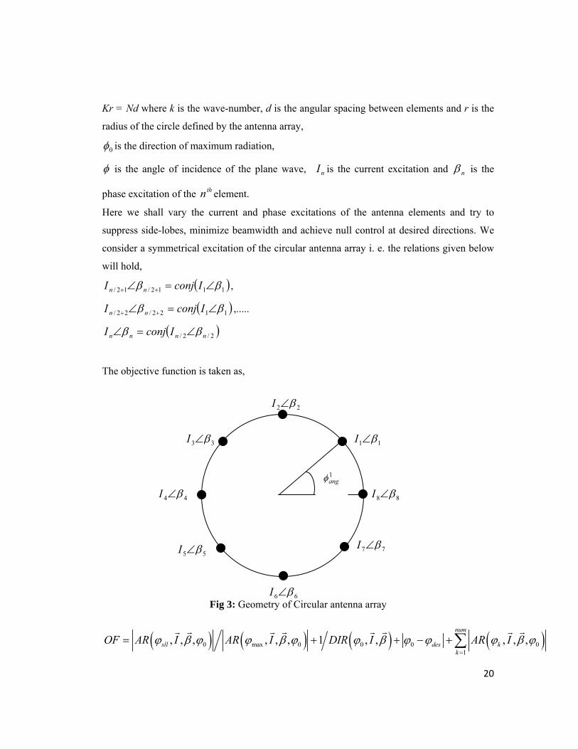
9. Circular Antenna Array Design Problem (Problem No. 10 in Table 1) Circular shaped antenna arrays find various applications in sonar, radar, mobile and
commercial satellite communication systems [21 – 23]. Let us consider N antenna elements
spaced on a circle of radius r in the x-y plane. This is shown in figure 1 and the antenna
elements are said to constitute a circular antenna array. The array factor for the circular array
is written as follows,
( ) ( ) ( )( )[ ]∑=
+−−−=N
nn
nang
nangn jkrIAF
10coscosexp βφφφφφ (52)
where,
( ) Nnnang 12 −= πφ is the angular position of the thn element on the x-y plane,
20
88 β∠I
77 β∠I 55 β∠I
33 β∠I
22 β∠I
11 β∠I
44 β∠I
66 β∠I
1angφ
Kr = Nd where k is the wave-number, d is the angular spacing between elements and r is the
radius of the circle defined by the antenna array,
0φ is the direction of maximum radiation,
φ is the angle of incidence of the plane wave, nI is the current excitation and nβ is the
phase excitation of the thn element.
Here we shall vary the current and phase excitations of the antenna elements and try to
suppress side-lobes, minimize beamwidth and achieve null control at desired directions. We
consider a symmetrical excitation of the circular antenna array i. e. the relations given below
will hold,
( )1112/12/ ββ ∠=∠ ++ IconjI nn ,
( )1122/22/ ββ ∠=∠ ++ IconjI nn ,.....
( )2/2/ nnnn IconjI ββ ∠=∠
The objective function is taken as,
Fig 3: Geometry of Circular antenna array
( ) ( ) ( ) ( )0 max 0 0 0 01
, , , , , , 1 , , , , ,num
sll des kk
OF AR I AR I DIR I AR Iϕ β ϕ ϕ β ϕ ϕ β ϕ ϕ ϕ β ϕ=
= + + − +∑r r r rr r r r
21
(53)
The first component attempts to suppress the sidelobes. sllφ is the angle at which maximum
sidelobe level is attained. The second component attempts to maximize directivity of the
array pattern. Nowadays directivity has become a very useful figure of merit for comparing
array patterns. The third component strives to drive the maxima of the array pattern close to
the desired maxima desφ . The fourth component penalizes the objective function if sufficient
null control is not achieved. num is the number of null control directions and kφ specifies the
thk null control direction.
Below we provide the instantiation of the design problem for this competition:
Number of elements in circular array = 12
x1= Any string within bounds
null= [50,120] in radians (no null control)
phi_desired= 180ο
distance= 0.5
Here x1 denotes the input string and the readers may look at the read_me.txt file in the folder
Prob_9_Circ_Antenna for more details.
10. Dynamic Economic Dispatch (DED) Problem (Problem No. 11.1 and 11.2 in Table 1)
The Dynamic Economic Dispatch (DED) problem follows the charecteristics of the hourly
dispatch problem, but here the power demand varies with each hour and the power generation
schedule for 24 hours is to be determined. We can say that the dimension of the DED
problem is 24 times that of the static ELD problem.
22
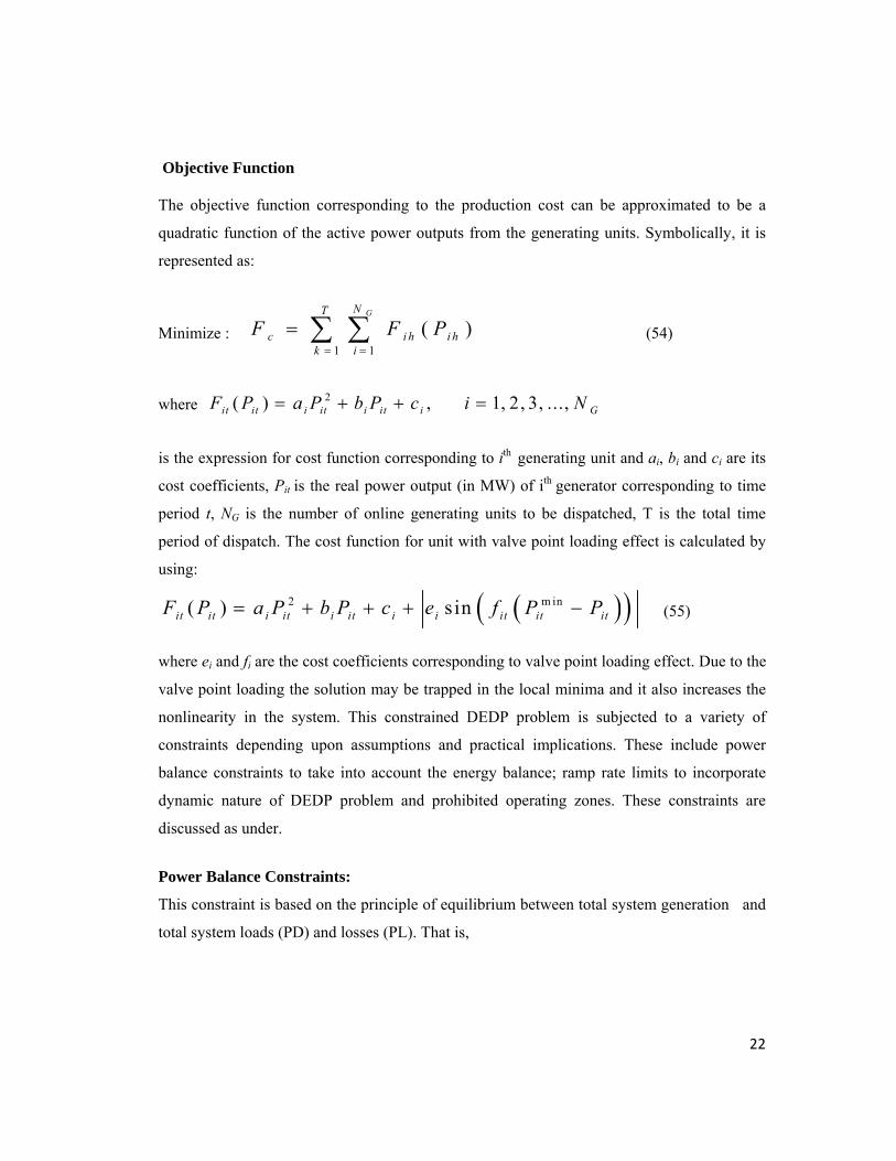
Objective Function The objective function corresponding to the production cost can be approximated to be a
quadratic function of the active power outputs from the generating units. Symbolically, it is
represented as:
Minimize : 1 1
( )GNT
c i h i hk i
F F P= =
= ∑ ∑ (54)
where 2( ) , 1, 2, 3, ...,it it i it i it i GF P a P b P c i N= + + =
is the expression for cost function corresponding to ith generating unit and ai, bi and ci are its
cost coefficients, Pit is the real power output (in MW) of ith generator corresponding to time
period t, NG is the number of online generating units to be dispatched, T is the total time
period of dispatch. The cost function for unit with valve point loading effect is calculated by
using:
( )( )2 m in( ) sinit it i it i it i i it it itF P a P b P c e f P P= + + + − (55)
where ei and fi are the cost coefficients corresponding to valve point loading effect. Due to the
valve point loading the solution may be trapped in the local minima and it also increases the
nonlinearity in the system. This constrained DEDP problem is subjected to a variety of
constraints depending upon assumptions and practical implications. These include power
balance constraints to take into account the energy balance; ramp rate limits to incorporate
dynamic nature of DEDP problem and prohibited operating zones. These constraints are
discussed as under.
Power Balance Constraints:
This constraint is based on the principle of equilibrium between total system generation and
total system loads (PD) and losses (PL). That is,

23
LtDt
N
iit PPP
G
+=∑=1
(56)
where PLt is obtained using B- coefficients, given by
∑ ∑= =
=G GN
i
N
jjtijitLt PBPP
1 1 (57)
Generator Constraints:
The output power of each generating unit has a lower and upper bound so that it lies in
between these bounds. This constraint is represented by a pair of inequality constraints as
follows:
maxmin
iiti PPP ≤≤ (58)
where, Pimin and Pi
max are lower and upper bounds for power outputs of the ith generating unit
in MW.
Ramp Rate Limits:
One of unpractical assumption that prevailed for simplifying the problem in many of the
earlier research is that the adjustments of the power output are instantaneous. However, under
practical circumstances ramp rate limit restricts the operating range of all the online units for
adjusting the generator operation between two operating periods. The generation may
increase or decrease with corresponding upper and downward ramp rate limits. So, units are
constrained due to these ramp rate limits as mentioned below.
If power generation increases, it
iit URPP ≤− −1
If power generation decreases, iitt
i DRPP ≤−−1
where Pit-1 is the power generation of unit i at previous hour and URi and DRi are the upper
and lower ramp rate limits respectively. The inclusion of ramp rate limits modifies the
generator operation constraints as follows
)DRP,Pmin(P)PUR,Pmax( i1t
imaxiiii
mini −≤≤− −
(59)
24
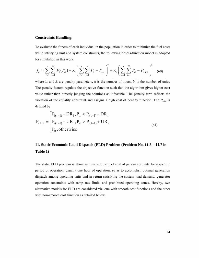
Constraints Handling:
To evaluate the fitness of each individual in the population in order to minimize the fuel costs
while satisfying unit and system constraints, the following fitness-function model is adopted
for simulation in this work: 2 2
1 lim1 1 1 1 1 1
( )n N n N n N
k i it it Dt r it rt i t i t i
f F P P P P Pλ λ= = = = = =
⎛ ⎞ ⎛ ⎞= + − + −⎜ ⎟ ⎜ ⎟
⎝ ⎠ ⎝ ⎠∑∑ ∑∑ ∑∑ (60)
where λ1 and λr are penalty parameters, n is the number of hours, N is the number of units.
The penalty factors regulate the objective function such that the algorithm gives higher cost
value rather than directly judging the solutions as infeasible. The penalty term reflects the
violation of the equality constraint and assigns a high cost of penalty function. The Prlim is
defined by
i(t 1) i it i( t 1) i
r lim i(t 1) i it i( t 1) i
it
P DR , P P DR
P P UR , P P UR
P , otherwise
− −
− −
− < −⎡⎢
= + > +⎢⎢⎣
(61)
11. Static Economic Load Dispatch (ELD) Problem (Problem No. 11.3 – 11.7 in
Table 1)
The static ELD problem is about minimizing the fuel cost of generating units for a specific
period of operation, usually one hour of operation, so as to accomplish optimal generation
dispatch among operating units and in return satisfying the system load demand, generator
operation constraints with ramp rate limits and prohibited operating zones. Hereby, two
alternative models for ELD are considered viz. one with smooth cost functions and the other
with non-smooth cost function as detailed below.

25
Objective Function
The objective function corresponding to the production cost can be approximated to be a
quadratic function of the active power outputs from the generating units. Symbolically, it is
represented as:
Minimize: 1
( )GN
i ii
F f P=
= ∑ (62)
where2( ) , 1,2,3, ...,i i i i i i i Gf P a P b P c i N= + + = is the expression for cost
function corresponding to ith generating unit and ai, bi and ci are its cost coefficients. Pi is the
real power output (in MW) of ith generator corresponding to time period t. NG is the number of
online generating units to be dispatched. The cost function for unit with valve point loading
effect is calculated by using:
( )( )iiiiiiiiiii PPfecPbPaPf −+++= min2 sin)( (63)
where ei and fi are the cost coefficients corresponding to valve point loading effect. This
constrained ELD problem is subjected to a variety of constraints depending upon assumptions
and practical implications. These include power balance constraints to take into account the
energy balance; ramp rate limits to incorporate dynamic nature of ELD problem and
prohibited operating zones. These constraints are discussed as under.
Power Balance Constraints or Demand Constraints
This constraint is based on the principle of equilibrium between total system generation and
total system loads (PD) and losses (PL). That is,
1
GN
i D Li
P P P=
= +∑ (64)
where PL is obtained using B- coefficients, given by
∑∑ ∑== =
++=GG G N
iii
N
i
N
jjijiL BPBPBPP
1000
1 1 (65)

26
Generator Constraints
The output power of each generating unit has a lower and upper bound so that it lies in
between these bounds. This constraint is represented by a pair of inequality constraints as
follows:
maxii
mini PPP ≤≤
(66)
where, Pimin and Pi
max are lower and upper bounds for power outputs of the ith generating unit.
Ramp Rate Limits
One of unpractical assumption that prevailed for simplifying the problem in many of the
earlier research is that the adjustments of the power outputs are unbounded. However, under
practical circumstances ramp rate limit restricts the operating range of all the online units for
adjusting the generator operation between two operating periods. The generation may
increase or decrease with corresponding upper and downward ramp rate limits. So, units are
constrained due to these ramp rate limits as mentioned below:
If power generation increases, i1t
ii URPP ≤− −
If power generation decreases, ii1t
i DRPP ≤−−
where Pit-1 is the power generation of unit i at previous hour and URi and DRi are the upper
and lower ramp rate limits respectively. The inclusion of ramp rate limits modifies the
generator operation constraints as follows:
)DRP,Pmin(P)PUR,Pmax( i1t
imaxiiii
mini −≤≤− −
Prohibited Operating Zones
The generating units may have certain zones where operation is restricted on the grounds of
physical limitations of machine components or instability e.g. due to steam valve or vibration
in shaft bearings. Consequently, discontinuities are produced in cost curves corresponding to

27
the prohibited operating zones. So, there is a quest to avoid operation in these zones in order
to economize the production. Symbolically, for a generating unit i,
PP and PP pzi
pzi
)(≥≤
where pzpz P and P)(
are the lower and upper limits of a given prohibited zone for
generating unit i.
Conflicts in Constraints Handling
If ever, the maximum or minimum limits of generation of a unit as given lie in the prohibited
zone for that generator, then some modifications are to be made in the upper and lower limits
for the generator constraints in order to avoid the conflicts. In case, maximum limit for a
generator lies in the prohibited zone, the lower limit of the prohibited zone is taken as the
maximum limit of power generation for that particular generator. Similarly, care is taken in
case the minimum limit of power generation of a generator lies in the prohibited zone by
taking upper limit of the prohibited zone as the lower limit of power generation for that
generator.
12. Hydrothermal Scheduling Problem (Problem No. 11.8 – 11.10 in Table 1)
Hydrothermal scheduling can be either a short term or a long term problem. Short term refers
to duration of typically 24 hours, while long term refers to duration of weeks or months. The
primary intent of short-term scheduling of a hydrothermal power system is to schedule the
power generations of the thermal and hydro units in the system to satiate the load demands, in
the scheduling duration of one day or a few days, in accordance with the various constraints
put on the hydraulic systems and the power system networks. Generally, the objective
function to be minimized in a hydrothermal scheduling problem is the overall fuel cost of
thermal units for the given short term. The hydrothermal system considered here is extremely
complex and involves nonlinear relationships of the decision variables, cascaded nature of
hydraulic network, water carry delays and time link between the consecutive schedules, that

28
make the problem of discovering global optimum cost difficult using regular optimization
methods.
The system considered comprises of a multi-chain cascaded network of four hydro plants and
an equivalent thermal power plant. If there are multiple thermal units, they can be taken
together and considered as an equivalent thermal network. The distribution of power among
those thermal units can be solved as a different and independent problem. Our objective here
would be to maximize the output of the hydro units such that thermal unit takes up only
minimum load. Considering the fact that we have to schedule the water discharges of four
hydro units for 24 hours, the dimension of the problem is 96. Such huge dimension can take
conventional methods years to solve using even a computer.
Objective Function
The total fuel cost for operation of the thermal system so as to meet the load demands in the
scheduling period is given by F . The objective function is formulated as
Minimize ( )Ti
M
1ii PfF ∑
=
= (67)
where fi is the cost function corresponding to the equivalent thermal unit’s power generation
PTi at ith interval . M is the total number of intervals considered for the short term schedule.
The cost function fi can be written as:
( )( )TiTiiiiTiiTiiTii PPfecPbPaPf −+++= min2 sin)( (68)
The minimization problem is subject to various system constraints.
Demand constraints
This constraint comes from the principle of energy conservation. The total power produced
by thermal unit and hydro units put together should be satiating both the power demand and
the power loss occurring.
29
Loss(i)D(i)
N
kH(k,i)T(i) PPPP +=+ ∑
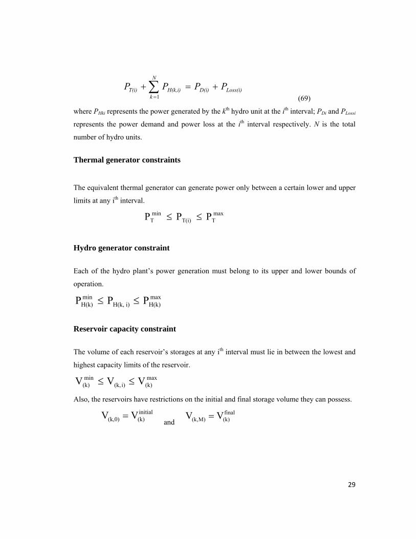
=1 (69)
where PHki represents the power generated by the kth hydro unit at the ith interval; PDi and PLossi
represents the power demand and power loss at the ith interval respectively. N is the total
number of hydro units.
Thermal generator constraints
The equivalent thermal generator can generate power only between a certain lower and upper
limits at any ith interval.
max
TT(i)min
T PPP ≤≤
Hydro generator constraint Each of the hydro plant’s power generation must belong to its upper and lower bounds of
operation.
maxH(k)i)H(k,
minH(k) PPP ≤≤
Reservoir capacity constraint
The volume of each reservoir’s storages at any ith interval must lie in between the lowest and
highest capacity limits of the reservoir.
max(k)i)(k,
min(k) VVV ≤≤
Also, the reservoirs have restrictions on the initial and final storage volume they can possess.
initial(k)(k,0) VV =
and final(k)M)(k, VV =
30
Water discharge constraint
The water discharge rate of each reservoir must belong to its minimum and maximum
operating limits at all intervals. max(k)i)(k,
min(k) QQQ ≤≤
Hydraulic continuity constraint
The volume stored in the kth reservoir for the (i+1)th interval is found from the following
continuity equation.
( ) i)(k,i)(k,i)(k,Ωj
τ)-i(j,τ)-i(j,i)(k,1)i(k, RSQSQVV(k)
+−−++= ∑=
+
(70)
where Ω(k) is the index set of the upstream reservoirs contributing to the kth reservoir, τ is the
time delay occurring for the water in jth upstream reservoir to reach the kth reservoir. S and R
represent the spillage and inflow rate respectively.
Hydro power generation equation
The hydro power generated by the kth unit at ith interval is taken as a function of discharge rate
and storage volume of that unit in that interval.
( )k)(6,i)(k,k)(5,i)(k,k)(4,
i)(k,i)(k,k)(3,2
i)(k,k)(2,2
i)(k,k)(1,i)H(k,
cQcVc
QVcQcVcP
+++
++=
(71)
where c(1,k) , c(2,k) , c(3,k) , c(4,k) , c(5,k) and c(6,k) are the constant coefficients of the system for the
kth reservoir.

31
13. Messenger: Spacecraft Trajectory Optimization Problem (Problem No. 12 in
Table 1)
A good benchmark to test global optimization algorithms in Space Mission Design related
problems is the Multiple Gravity Assist (MGA) problem. In mathematical terms this is a
finite dimension global optimisation problem with non linear constraints. It can be used to
locate the best possible trajectory that an interplanetary probe equipped with a chemical
propulsion engine may take to go from the Earth to another planet or asteroid. The spacecraft
is constrained to thrust only at planetary encounters. A detailed description of the problem
may be found in [24]. The constraint on the spacecraft thrusting only only at planetary
encounters is often unacceptable as it may results in trajectories that are not realistic or that
use more propellant than necessary. The MGA-1DSM problem removes most of these
limitations. It represents an interplanetary trajectory of a spacecraft equipped with chemical
propulsion, able to thrust its engine once at any time during each trajectory leg. Thus the
solutions to this problem are suitable to perform preliminary quantitative calculation for real
space missions. This comes to the price of having to solve an optimization problem of larger
dimensions. The implementation details of this problem are the sum of a number of
previously published works [25 - 28].
The “Messenger” trajectory optimization problem represents a rendezvous mission to
Mercury modeled as an MGA-1DSM problem. The selected fly-by sequence and other
parameters are compatible with the currently flying Messenger mission. With respect to the
problem "Messenger" the fly-by sequence is more complex and allows for resonant fly-bys at
Mercury to lower the arrival DV. For the twenty-six dimensional global optimization
problem, the detailed ranges of each variable, MATLAB codes etc. can be found from the
URL:
http://www.esa.int/gsp/ACT/inf/op/globopt/MessengerFull.html

32
14. Cassini 2: Spacecraft Trajectory Optimization Problem (Problem No. 13 in
Table 1)
In this problem the objective function (unconstrained) evaluates the DV required to reach
Saturn using an Earth – Venus, Venus – Earth, Jupiter - Saturn fly-by sequence with deep
space maneuvers. Consider a different model for the Cassini trajectory: deep space maneuvers
are allowed between each one of the planets. This leads to a higher dimensional problem with
a much higher complexity. We also consider, in the objective function evaluation, a
rendezvous problem rather than an orbital insertion as in the MGA model of the Cassini
mission. This is the main cause for the higher objective function values reached. For the 12-
dimensional state-vector the bounds, the MATLAB code for evaluating the objective
functions etc. can be found in the following URL:
http://www.esa.int/gsp/ACT/inf/op/globopt/edvdvdedjds.htm
33
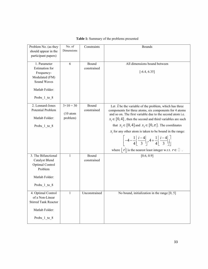
Table 1: Summary of the problems presented
Problem No. (as they should appear in the participant papers)
No. of Dimensions
Constraints Bounds
1. Parameter Estimation for
Frequency-Modulated (FM)
Sound Waves
Matlab Folder:
Probs_1_to_8
6 Bound constrained
All dimensions bound between
[-6.4, 6.35]
2. Lennard-Jones Potential Problem
Matlab Folder:
Probs_1_to_8
3×10 = 30
(10 atom problem)
Bound constrained
Let xr be the variable of the problem, which has three components for three atoms, six components for 4 atoms and so on. The first variable due to the second atom i.e.
1 [0, 4]x ∈ , then the second and third variables are such
that 2 [0, 4]x ∈ and 3 [0, ]x π∈ . The coordinates
ix for any other atom is taken to be bound in the range:
1 4 1 44 ,44 3 4 3
i i⎡ ⎤− −⎢ ⎥ ⎢ ⎥− − +⎢ ⎥⎢ ⎥ ⎢ ⎥⎣ ⎦ ⎣ ⎦⎣ ⎦
where r⎢ ⎥⎣ ⎦ is the nearest least integer w.r.t. r∈ .
3. The Bifunctional Catalyst Blend
Optimal Control Problem
Matlab Folder:
Probs_1_to_8
1 Bound constrained
[0.6, 0.9]
4. Optimal Control of a Non-Linear
Stirred Tank Reactor
Matlab Folder:
Probs_1_to_8
1 Unconstrained No bound, initialization in the range [0, 5]

34
5. Tersoff Potential for model Si (B)
Matlab Folder:
Probs_1_to_8
and
6. Tersoff Potential for model Si (C)
Matlab Folder:
Probs_1_to_8
3×10 = 30
(10 atom problem)
Bound constrained
Let xr be the variable of the problem which has three components for three atoms, six components for 4 atoms and so on. The first variable due to the second atom i.e.
1 [0, 4]x ∈ , then the second and third variables are such
that 2 [0, 4]x ∈ and 3 [0, ]x π∈ . The coordinates
ix for any other atom is taken to be bound in the range:
1 4 1 44 ,44 3 4 3
i i⎡ ⎤− −⎢ ⎥ ⎢ ⎥− − +⎢ ⎥⎢ ⎥ ⎢ ⎥⎣ ⎦ ⎣ ⎦⎣ ⎦
where r⎢ ⎥⎣ ⎦ is the nearest least integer w.r.t. r∈ .
7. Spread Spectrum Radar Polly phase
Code Design
Matlab Folder:
Probs_1_to_8
20 Bound constrained
All dimensions bound between
[0, 2 ]π
8. Transmission Network Expansion Planning (TNEP)
Problem:
Matlab Folder:
Probs_1_to_8
7 Equality and inequality constraints
All variables are bounded in the interval [0, 15].
9. Large Scale Transmission Pricing
Problem
Matlab Folder:
Prob_9_Transmission_Pricing
g*d (g: no. of
generator buses, d:
no. of load buses)
For, IEEE 30 bus system:
g=6, d=21
Linear Equality
Constraints
max min ,
min 0ij gi ij dj ij
ij
GD P BT P BT
GD
= − −
=
(plz see the bounds.m file in \Prob_8_Transmission_Pricing folder)
10. Circular Antenna Array Design
Problem
12 Bound constrained
First six dimensions in [0.2, 1] and next six dimensions [-180, 180]
35
Matlab Folder:
Prob_10_Circ_Antenna
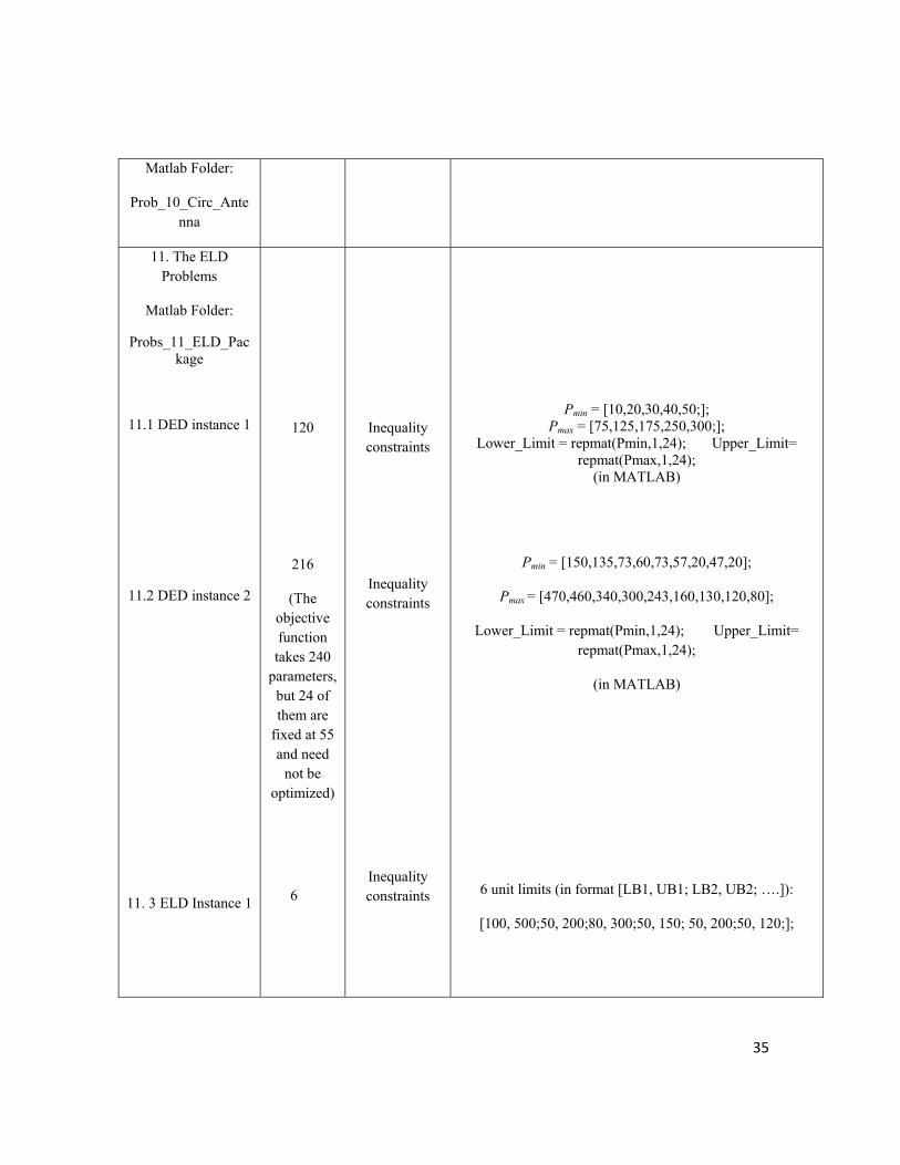
11. The ELD Problems
Matlab Folder:
Probs_11_ELD_Package
11.1 DED instance 1
11.2 DED instance 2
11. 3 ELD Instance 1
120
216
(The objective function takes 240
parameters, but 24 of them are
fixed at 55 and need
not be optimized)
6
Inequality constraints
Inequality constraints
Inequality constraints
Pmin = [10,20,30,40,50;]; Pmax = [75,125,175,250,300;];
Lower_Limit = repmat(Pmin,1,24); Upper_Limit= repmat(Pmax,1,24);
(in MATLAB)
Pmin = [150,135,73,60,73,57,20,47,20];
Pmax = [470,460,340,300,243,160,130,120,80];
Lower_Limit = repmat(Pmin,1,24); Upper_Limit= repmat(Pmax,1,24);
(in MATLAB)
6 unit limits (in format [LB1, UB1; LB2, UB2; ….]):
[100, 500;50, 200;80, 300;50, 150; 50, 200;50, 120;];
36
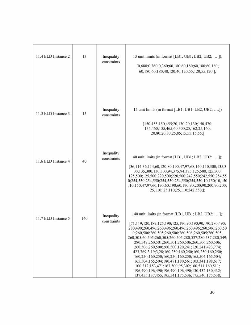
11.4 ELD Instance 2
11.5 ELD Instance 3
11.6 ELD Instance 4
11.7 ELD Instance 5
13
15
40
140
Inequality constraints
Inequality constraints
Inequality constraints
Inequality constraints
13 unit limits (in format [LB1, UB1; LB2, UB2; ….]):
[0,680;0,360;0,360;60,180;60,180;60,180;60,180; 60,180;60,180;40,120;40,120;55,120;55,120;];
15 unit limits (in format [LB1, UB1; LB2, UB2; ….])
[150,455;150,455;20,130;20,130;150,470; 135,460;135,465;60,300;25,162;25,160;
20,80;20,80;25,85;15,55;15,55;]
40 unit limits (in format [LB1, UB1; LB2, UB2; ….]):
[36,114;36,114;60,120;80,190;47,97;68,140;110,300;135,300;135,300;130,300;94,375;94,375;125,500;125,500;
125,500;125,500;220,500;220,500;242,550;242,550;254,550;254,550;254,550;254,550;254,550;254,550;10,150;10,150;10,150;47,97;60,190;60,190;60,190;90,200;90,200;90,200;
25,110; 25,110;25,110;242,550;];
140 unit limits (in format [LB1, UB1; LB2, UB2; ….]):
[71,119;120,189;125,190;125,190;90,190;90,190;280,490; 280,490;260,496;260,496;260,496;260,496;260,506;260,50
9;260,506;260,505;260,506;260,506;260,505;260,505; 260,505;60,505;260,505;260,505;280,537;280,537;280,549;
280,549;260,501;260,501;260,506;260,506;260,506; 260,506;260,500;260,500;120,241;120,241;423,774;
423,769;3,19;3,28;160,250;160,250;160,250;160,250; 160,250;160,250;160,250;160,250;165,504;165,504; 165,504;165,504;180,471;180,561;103,341;198,617; 100,312;153,471;163,500;95,302;160,511;160,511; 196,490;196,490;196,490;196,490;130,432;130,432; 137,455;137,455;195,541;175,536;175,540;175,538;

37
11.8 Hydrothermal Scheduling Instance
1
11.9 Hydrothermal Scheduling Instance
2
11.10 Hydrothermal Scheduling Instance
3
96
96
96
Inequality constraints
Inequality constraints
Inequality constraints
175,540;330,574;160,531;160,531;200,542;56,132; 115,245;115,245;115,245;207,307;207,307;175,345; 175,345;175,345;175,345;360,580;415,645;795,984; 795,978;578,682;615,720;612,718;612,720;758,964;
755,958;750,1007;750,1006;713,1013;718,1020;791,954; 786,952;795,1006;795,1013;795,1021;795,1015;94,203; 94,203;94,203;244,379;244,379;244,379;95,190;95,189;
116,194;175,321;2,19;4,59;15,83;9,53;12,37;10,34; 112,373;4,20;5,38;5,19;50,98;5,10;42,74;42,74;
41,105;17,51;7,19;7,19;26,40;];
Qmin = [5 6 10 13]; Qmax = [15 15 30 25]; Lower_Limit = repmat(Qmin,1,24);
Upper_Limit = repmat(Qmax, 1, 24);
Same as 11.8
Same as 11.8
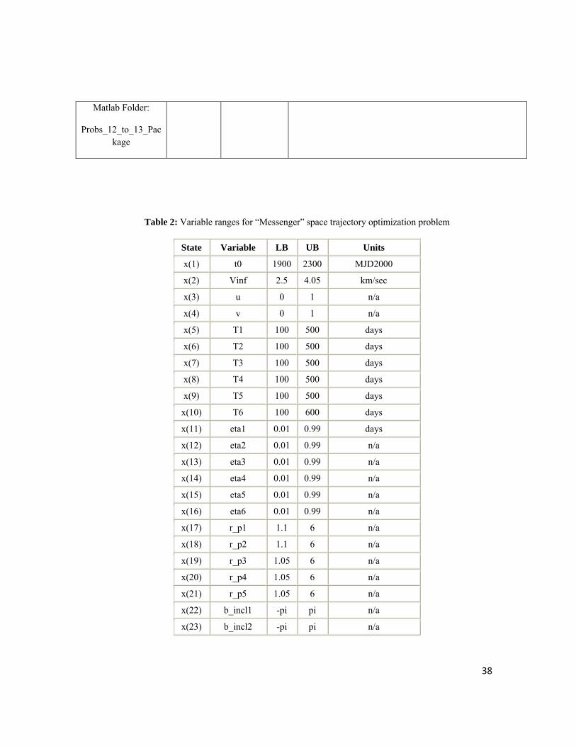
12. Messenger: Spacecraft Trajectory
Optimization Problem
Matlab Folder:
Probs_12_to_13_Package
26 Bound constraints
Please see Table 2
13. Cassini 2: Spacecraft Trajectory
Optimization Problem
22 Bound constraints
Please see Table 3
38
Matlab Folder:
Probs_12_to_13_Package
Table 2: Variable ranges for “Messenger” space trajectory optimization problem
State Variable LB UB Units
x(1) t0 1900 2300 MJD2000
x(2) Vinf 2.5 4.05 km/sec
x(3) u 0 1 n/a
x(4) v 0 1 n/a
x(5) T1 100 500 days
x(6) T2 100 500 days
x(7) T3 100 500 days
x(8) T4 100 500 days
x(9) T5 100 500 days
x(10) T6 100 600 days
x(11) eta1 0.01 0.99 days
x(12) eta2 0.01 0.99 n/a
x(13) eta3 0.01 0.99 n/a
x(14) eta4 0.01 0.99 n/a
x(15) eta5 0.01 0.99 n/a
x(16) eta6 0.01 0.99 n/a
x(17) r_p1 1.1 6 n/a
x(18) r_p2 1.1 6 n/a
x(19) r_p3 1.05 6 n/a
x(20) r_p4 1.05 6 n/a
x(21) r_p5 1.05 6 n/a
x(22) b_incl1 -pi pi n/a
x(23) b_incl2 -pi pi n/a

39
x(24) b_incl3 -pi pi n/a
x(25) b_incl4 -pi pi n/a
x(26) b_incl5 -pi pi n/a
Table 3: Variable ranges for “Cassini 2” space trajectory optimization problem
State Variable LB UB Units x(1) t0 -1000 0 MJD2000 x(2) Vinf 3 5 km/sec x(3) u 0 1 n/a x(4) v 0 1 n/a x(5) T1 100 400 days x(6) T2 100 500 days x(7) T3 30 300 days x(8) T4 400 1600 days x(9) T5 800 2200 days x(10) eta1 0.01 0.9 n/a x(11) eta2 0.01 0.9 n/a x(12) eta3 0.01 0.9 n/a x(13) eta4 0.01 0.9 n/a x(14) eta5 0.01 0.9 n/a x(15) r_p1 1.05 6 n/a x(16) r_p2 1.05 6 n/a x(17) r_p3 1.15 6.5 n/a x(18) r_p4 1.7 291 n/a x(19) b_incl1 -pi pi rad x(20) b_incl2 -pi pi rad x(21) b_incl3 -pi pi rad x(22) b_incl4 -pi pi rad
2. Evaluation Criteria
40
The authors should report the mean, best, and worst objective function values
obtained over 25 independent runs. The authors are asked to report these values after
executing their algorithms for 50000, 100000, and 150000 FEs (Function
Evaluations). The participants should use uniform random initialization within the
prescribed search space for each problem. We discourage participants searching for a
distinct set of parameters for each problem/dimension/etc. Please provide details on
the following whenever applicable:
a) All parameters to be adjusted
b) Corresponding dynamic ranges
c) Guidelines on how to adjust the parameters
d) Estimated cost of parameter tuning in terms of number of FEs
e) Actual parameter values used.
If the algorithm requires encoding, then the encoding scheme should be independent
of the specific problems and governed by generic factors such as the search ranges.
References:
[1] Horner, J. Beauchamp, and L. Haken, “Genetic algorithms and their application to FM matching
synthesis,” Comput. Music J., vol. 17, no. 4, pp. 17–29, 1993.
[2] F. Herrera and M. Lozano, “Gradual distributed real-coded genetic algorithms,” IEEE Trans. Evol.
Comput., vol. 4, no. 1, pp. 43–62, Apr. 2000.
[3] M.R. Hoare, “Structure and dynamics of simple microclusters”, Advances in Chemical Physics,
Vol. 40, pp. 49-135, 1979.
[4] N. P. Moloi and M. M. Ali, "An Iterative Global Optimization Algorithm for Potential Energy
Minimization", Journal of Computational Optimization and Applications, 30 (2), 119-132, 2005.
[5] G. L. Xue, R. S. Maier, and J. B. Rosen, Minimizing the Lennard-Jones potential function on a
massively parallel computer, Preprint 91-115, AHPCRC, University of Minnesota, Minneapolis,
MN, 1991.
41
[6] R. Luus and B. Bojkov, “Global optimization of the bifunctional catalyst problem”, Can. J. Chem.
Eng. 72, pp.160–163, 1994.
[7] R. Luus, Iterative Dynamic Programming, Chapman & Hall/CRC Press, Boca Raton, FL, 2000.
[8] W.R. Esposito and C. A. Floudas, “Deterministic global optimization in non-linear optimal control
problems”, J. Global Optim. 17, pp. 97–126, 2000.
[9] C .A. Floudas, P. M. Pardalos, C. S. Adjiman, W. R. Esposito, Z. H. Gumus, S.T. Harding, J. L.
Klepeis, C. A. Meyer, C. A. Schweiger, “Handbook of test problems in local and global
optimization”, Kluwer Academic Publishers, Dordrecht, The Netherlands, 1996.
[10] M.M. Ali, C. Storey, and A. Törn, “Application of stochastic global optimization algorithms to
practical problems”, J. Optim. Theory Applic. 95 (3), pp. 545–563, 1997.
[11] J. Tersoff, (1988), Empirical interatomic potential for silicon with improved elastic properties,
Physics Review B, 38:9902-9905.
[12] M. M. Ali and A. Torn, A. (2000), Optimization of carbon and silicon cluster geometry for
Tersoff potential using differential evolution, in Optimization in Computational Chemistry and
Molecular Biology: Local and Global Approaches, Edited by A. Floudas and M. Pardalos,
Kluwer Academic Publisher, 287-300.
[13] M.L. Dukic and Z.S. Dobrosavljevic, “A method of a spreadspectrum radar polyphase code
design”, IEEE Journal on Selected Areas in Comm. 8, pp. 743–749, 1990.
[14] N. Mladenović, J. Petrovic, V. Kovacevic-Vujicic, and M. Cangalovic, “Solving spread-
spectrum radar polyphase code design problem by tabu search and variable neighborhood
search,” European Journal of Operational Research, 153, 389-399, 2003.
[15] S. Das, A. Konar, U. K. Chakraborty, and A. Abraham, “Differential evolution with a
neighborhood based mutation operator: a comparative study”, IEEE Transactions on
Evolutionary Computation, Vol. 13, Issue 3, Page(s): 526-553, June, 2009.
[16] B. K. Panigrahi, A. Abraham, and S. Das (Eds.), Computational Intelligence in Power
Engineering, Springer-Verlag Berlin Heidelberg, SCI 302, pp. 367 – 379, 2010.
[17] I. J. De Silva, IM. J. Rider, R. Romero, A. V. Garcia, and C. A. Murari, “Transmission network
expansion planning with security constraints”, IEE Proc. Gener. Transm. Distrib. 152(6), pp.
828–836, 2005.
[18] R. D. Christie, B. F..Wollenberg, and I. Wangensteen, “Transmission management in
deregulated environment”, Proc. IEEE, Vol. 88, pp. 170-195, FEB 2000.
[19] F. D. Galiana, A J. Conejo, and H A. Gil, “Transmission network cost allocation based on
Equivalent Bilateral Exchanges”, IEEE Trans. on Power Systems, vol. 18, no. 4, Nov. 2003.

42
[20] Y. M. Park, J. U. Lim, and J. R. Won, “An analytical approach for transmission costs allocation
in transmission system”, IEEE Trans. on Power Systems, vol. 13, no. 4, pp. 1407-1412, Nov.
2003.
[21] M. I. H. Dessouky, A. Sharshar, and Y. A. Albagory, “Efficient sidelobe reduction technique for
small-sized concentric circular arrays," Progress In Electromagnetics Research, PIER 65, 187 -
200, 2006.
[22] L. Gurel and O. Ergul, “Design and simulation of circular arrays of trapezoidal-tooth log-
periodic antennas via genetic optimization," Progress In Electromagnetics Research, PIER 85,
243 - 260, 2008.
[23] M. Dessouky, H. Sharshar, and Y. Albagory, “A novel tapered beamforming window for uniform
concentric circular arrays," Journal of Electromagnetic Waves and Applications, Vol. 20, No.
14, 2077 -2089, 2006.
[24] Addis, B. and Cassioli, A. and Locatelli, M. and and Schoen, F. Global optimization for the design of space trajectories. COAP, submitted, 2008. published: Optimization On Line.
[25] D. Izzo, Global optimization and space pruning for spacecraft trajectory design, In Spacecraft Trajectory Optimization (Conway Ed.), Cambridge University Press, 2009.
[26] A. Cassioli, D. Di Lorenzo, M. Locatelli, F. Schoen, and M. Sciandrone, “Machine learning for global optimization” in e-prints for the optimization community (http://www.optimization-online.org/DB_FILE/2009/08/2360.pdf)
[27] M. Schlueter, J. J. Rückmann, and M. Gerdts, “Non-linear mixed-integer-based Optimization Technique for Space Applications”, Poster for ESA NPI Day 2010.
[28] T. Vinkó and D. Izzo, “Global optimisation heuristics and test problems for preliminary spacecraft trajectory design, european space agency”, The Advanced Concepts Team, ACT technical report (GOHTPPSTD), 2008.
Top Related