


Languages
Pages
Legal

Probability and Statistics NotesChapter Five
Jesse Crawford
Department of MathematicsTarleton State University
Spring 2011
(Tarleton State University) Chapter Five Notes Spring 2011 1 / 37
Outline
1 Section 5.2: Transformations of Two Random Variables
2 Section 5.3: Several Independent Random Variables
3 Section 5.4: The Moment-Generating Function Technique
4 Section 5.5: Random Functions Associated with NormalDistributions
5 Section 5.6: The Central Limit Theorem
6 Section 5.7: Approximations for Discrete Distributions
7 Review for Exam 1
(Tarleton State University) Chapter Five Notes Spring 2011 2 / 37
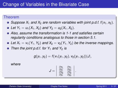
Change of Variables in the Bivariate Case
TheoremSuppose X1 and X2 are random variables with joint p.d.f. f (x1, x2).Let Y1 = u1(X1,X2) and Y2 = u2(X1,X2).Also, assume the transformation is 1-1 and satisfies certainregularity conditions analogous to those in section 5.1.Let X1 = v1(Y1,Y2) and X2 = v2(Y1,Y2) be the inverse mappings.Then the joint p.d.f. for Y1 and Y2 is
g(y1, y2) = f (v1(y1, y2), v2(y1, y2))|J|,
where
J =
∣∣∣∣∣ ∂x1∂y1
∂x1∂y2
∂x2∂y1
∂x2∂y2
∣∣∣∣∣ .(Tarleton State University) Chapter Five Notes Spring 2011 3 / 37

The F Distribution
DefinitionSuppose U and V are independent, andU ∼ χ2(r1) and V ∼ χ2(r2).Then the random variable
W =U/r1
V/r2
is said to have an F distribution with r1 and r2 degrees of freedom,denoted F (r1, r2).If 0 < α < 1, then Fα(r1, r2) is the critical value such that
P[W ≥ Fα(r1, r2)] = α.
(Tarleton State University) Chapter Five Notes Spring 2011 4 / 37
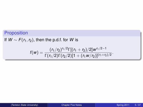
PropositionIf W ∼ F (r1, r2), then the p.d.f. for W is
f (w) =(r1/r2)r1/2Γ[(r1 + r2)/2]w r1/2−1
Γ(r1/2)Γ(r2/2)[1 + (r1w/r2)](r1+r2)/2 .
(Tarleton State University) Chapter Five Notes Spring 2011 5 / 37
Outline
1 Section 5.2: Transformations of Two Random Variables
2 Section 5.3: Several Independent Random Variables
3 Section 5.4: The Moment-Generating Function Technique
4 Section 5.5: Random Functions Associated with NormalDistributions
5 Section 5.6: The Central Limit Theorem
6 Section 5.7: Approximations for Discrete Distributions
7 Review for Exam 1
(Tarleton State University) Chapter Five Notes Spring 2011 6 / 37

Independence and Random Samples
DefinitionSuppose X1, . . . ,Xn are random variables with joint p.d.f.f (x1, . . . , xn), andlet fi(xi) be the p.d.f. of Xi , for i = 1, . . . ,n.Then X1, . . . ,Xn are independent if
f (x1, . . . , xn) = f1(x1) · · · fn(xn).
If these random variables all have the same distribution, they aresaid to be identically distributed.If X1, . . . ,Xn are independent and identically distributed (IID), thenthey are referred to as a random sample of size n from theircommon distribution.
(Tarleton State University) Chapter Five Notes Spring 2011 7 / 37
ExampleA certain population of women have heights that are normallydistributed,with mean 64 inches and standard deviation 2 inches.Let (X1,X2,X3) be a random sample of size 3 from this population.Find the joint p.d.f. for (X1,X2,X3).Find the probability that everyone’s height in the sample exceeds67 inches.
(Tarleton State University) Chapter Five Notes Spring 2011 8 / 37
PropositionIf X1, . . . ,Xn are independent, then for any sets A1, . . . ,An,
P(X1 ∈ A1, . . . ,Xn ∈ An) = P(X1 ∈ A1) · · ·P(Xn ∈ An)
Also, for any functions u1, . . . ,un,
E [u1(X1) · · · un(Xn)] = E [u1(X1)] · · ·E [un(Xn)]
(Tarleton State University) Chapter Five Notes Spring 2011 9 / 37

Mean and Variance of a Linear Combination of R.V.’s
TheoremSuppose X1, . . . ,Xn are independent R.V.’swith means µ1, . . . , µn, andvariances σ2
1, . . . , σ2n.
If a1, . . . ,an ∈ R, then
E [a1X1 + · · ·+ anXn] = a1µ1 + · · ·+ anµn, and
Var[a1X1 + · · ·+ anXn] = a21σ
21 + · · ·+ a2
nσ2n.
(Tarleton State University) Chapter Five Notes Spring 2011 10 / 37
Mean and Variance of the Sample Mean
DefinitionLet X1, . . . ,Xn be a random sample.The sample mean is
X =1n
n∑i=1
Xi .
PropositionLet X1, . . . ,Xn be a random sample from a population withpopulation mean µ and population variance σ2.Then
E(X ) = µ, and
Var(X ) =σ2
n.
(Tarleton State University) Chapter Five Notes Spring 2011 11 / 37

Outline
1 Section 5.2: Transformations of Two Random Variables
2 Section 5.3: Several Independent Random Variables
3 Section 5.4: The Moment-Generating Function Technique
4 Section 5.5: Random Functions Associated with NormalDistributions
5 Section 5.6: The Central Limit Theorem
6 Section 5.7: Approximations for Discrete Distributions
7 Review for Exam 1
(Tarleton State University) Chapter Five Notes Spring 2011 12 / 37

m.g.f. of a Linear Combination
Theorem (5.4-1)Suppose X1, . . . ,Xn are independent R.V.’s withmoment-generating functions MXi (t), for i = 1, . . . ,n.Then the moment-generating function of Y =
∑ni=1 aiXi is
MY (t) =n∏
i=1
MXi (ai t).
Example (5.4-2)Suppose 0 ≤ p ≤ 1, andX1, . . . ,Xn all have a Bernoulli(p) distribution.Find the distribution of Y =
∑ni=1 Xi .
(Tarleton State University) Chapter Five Notes Spring 2011 13 / 37

Corollaries for Random Samples
Corollary (5.4-1)Suppose X1, . . . ,Xn is a random samplefrom a distribution with m.g.f. M(t).Then the m.g.f. of Y =
∑ni=1 Xi is
MY (t) = [M(t)]n, and
the m.g.f. of X is
MX (t) =
[M(
tn
)]n
.
Example (5.4-3)Suppose (X1,X2,X3) is a random sample froman exponential distribution with mean θ.Find the distributions of Y = X1 + X2 + X3 and X .
(Tarleton State University) Chapter Five Notes Spring 2011 14 / 37

Theorem (5.4-2)If X1, . . . ,Xn are independent, andXi ∼ χ2(ri), for each i, then
X1 + · · ·+ Xn ∼ χ2(r1 + · · ·+ rn).
Corollary (5.4-2)If Z1, . . . ,Zn are independent standard normal R.V.’s, then
W = Z 21 + · · ·+ Z 2
n ∼ χ2(n).
Corollary (5.4-3)
If X1, . . . ,Xn are independent, and each Xi ∼ N(µi , σ2i ), then
W =n∑
i=1
(Xi − µi)2
σ2i
∼ χ2(n).
(Tarleton State University) Chapter Five Notes Spring 2011 15 / 37

Outline
1 Section 5.2: Transformations of Two Random Variables
2 Section 5.3: Several Independent Random Variables
3 Section 5.4: The Moment-Generating Function Technique
4 Section 5.5: Random Functions Associated with NormalDistributions
5 Section 5.6: The Central Limit Theorem
6 Section 5.7: Approximations for Discrete Distributions
7 Review for Exam 1
(Tarleton State University) Chapter Five Notes Spring 2011 16 / 37
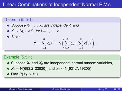
Linear Combinations of Independent Normal R.V.’s
Theorem (5.5-1)Suppose X1, . . . ,Xn are independent, andXi ∼ N(µi , σ
2i ), for i = 1, . . . ,n.
Then
Y =n∑
i=1
ciXi ∼ N
(n∑
i=1
ciµi ,
n∑i=1
c2i σ
2i
).
Example (5.5-1)Suppose X1 and X2 are independent normal random variables,X1 ∼ N(693.2,22820), and X2 ∼ N(631.7,19205).Find P(X1 > X2).
(Tarleton State University) Chapter Five Notes Spring 2011 17 / 37

Sample Mean and Variance for a Normal Population
Theorem (5.5-2)
Let (X1, . . . ,Xn) be a random sample from N(µ, σ2).Then the sample mean
X =1n
n∑i=1
Xi ,
and the sample variance,
S2 =1
n − 1
n∑i=1
(Xi − X )2,
are independent. Their distributions are
X ∼ N(µ, σ2/n), and S2 ∼ σ2
n − 1χ2(n − 1).
(Tarleton State University) Chapter Five Notes Spring 2011 18 / 37

ExampleConsider a population of women whose heights arenormally distributed with mean 64 inchesand standard deviation 2 inches.For a sample of size n = 10, find P(63 < X < 65), andfind constants a and b such that P(a < S2 < b) = 0.95.Repeat the problem when n = 81.
(Tarleton State University) Chapter Five Notes Spring 2011 19 / 37

Unbiasedness of X and S2
From Theorem 5.5-2, we have
E [X ] = µ, and E [S2] = σ2.
X , the sample mean, is used to estimate the population mean µ.S2, the sample variance, is used to estimate the populationvariance σ2.On average, each of these estimators are equal to the parametersthey are intended to estimate.That is, X and S2 are unbiased.
(Tarleton State University) Chapter Five Notes Spring 2011 20 / 37

Remarks about Degrees of Freedom
In the proof of Theorem 5.5-2, we noted that
n∑i=1
(Xi − µ)2
σ2 ∼ χ2(n), and
n∑i=1
(Xi − X )2
σ2 ∼ χ2(n − 1).
Replacing the parameter µ with its estimator X resulted in a lossof one degree of freedom.There are many examples where the degrees of freedom isreduced by one for each parameter being estimated.
(Tarleton State University) Chapter Five Notes Spring 2011 21 / 37
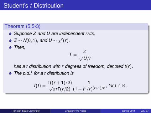
Student’s t Distribution
Theorem (5.5-3)Suppose Z and U are independent r.v.’s,Z ∼ N(0,1), and U ∼ χ2(r).Then,
T =Z√U/r
has a t distribution with r degrees of freedom, denoted t(r).The p.d.f. for a t distribution is
f (t) =Γ((r + 1)/2)√πrΓ(r/2)
1(1 + t2/r)(r+1)/2 , for t ∈ R.
(Tarleton State University) Chapter Five Notes Spring 2011 22 / 37

Relevance to Samples from Normal Distributions
Corollary
Suppose X1, . . . ,Xn is a random sample from N(µ, σ2).Then
T =X − µS/√
n
has a t distribution with n − 1 degrees of freedom.
(Tarleton State University) Chapter Five Notes Spring 2011 23 / 37

Outline
1 Section 5.2: Transformations of Two Random Variables
2 Section 5.3: Several Independent Random Variables
3 Section 5.4: The Moment-Generating Function Technique
4 Section 5.5: Random Functions Associated with NormalDistributions
5 Section 5.6: The Central Limit Theorem
6 Section 5.7: Approximations for Discrete Distributions
7 Review for Exam 1
(Tarleton State University) Chapter Five Notes Spring 2011 24 / 37
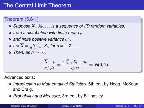
The Central Limit Theorem
Theorem (5.6-1)Suppose X1,X2, . . . is a sequence of IID random variables,from a distribution with finite mean µand finite positive variance σ2.Let X = 1
n∑n
i=1 Xi , for n = 1,2, . . .Then, as n→∞,
X − µσ/√
n=
∑ni=1 Xi − nµ√
nσ⇒ N(0,1).
Advanced texts:Introduction to Mathematical Statistics, 6th ed., by Hogg, McKean,and Craig.Probability and Measure, 3rd ed., by Billingsley.
(Tarleton State University) Chapter Five Notes Spring 2011 25 / 37
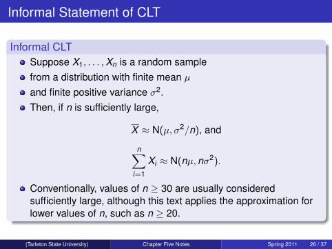
Informal Statement of CLT
Informal CLTSuppose X1, . . . ,Xn is a random samplefrom a distribution with finite mean µand finite positive variance σ2.Then, if n is sufficiently large,
X ≈ N(µ, σ2/n), and
n∑i=1
Xi ≈ N(nµ,nσ2).
Conventionally, values of n ≥ 30 are usually consideredsufficiently large, although this text applies the approximation forlower values of n, such as n ≥ 20.
(Tarleton State University) Chapter Five Notes Spring 2011 26 / 37
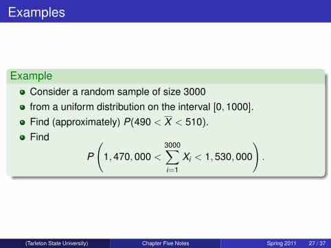
Examples
ExampleConsider a random sample of size 3000from a uniform distribution on the interval [0,1000].Find (approximately) P(490 < X < 510).Find
P
(1,470,000 <
3000∑i=1
Xi < 1,530,000
).
(Tarleton State University) Chapter Five Notes Spring 2011 27 / 37

Lottery Tickets
ExampleConsider a $1 scratch-off lottery ticket with the following prizestructure:
Prize($) Probability0 0.802 0.15
10 0.05
Find the expected profit/loss from buying a single ticket. Also findthe standard deviation.What is the chance of breaking even if you buy one ticket?If you buy 100 tickets?If you buy 500 tickets?
(Tarleton State University) Chapter Five Notes Spring 2011 28 / 37
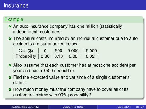
Insurance
ExampleAn auto insurance company has one million (statisticallyindependent) customers.The annual costs incurred by an individual customer due to autoaccidents are summarized below:
Cost($) 0 500 5,000 15,000Probability 0.80 0.10 0.08 0.02
Also, assume that each customer has at most one accident peryear and has a $500 deductible.Find the expected value and variance of a single customer’sclaims.How much money must the company have to cover all of itscustomers’ claims with 99% probability?
(Tarleton State University) Chapter Five Notes Spring 2011 29 / 37
Outline
1 Section 5.2: Transformations of Two Random Variables
2 Section 5.3: Several Independent Random Variables
3 Section 5.4: The Moment-Generating Function Technique
4 Section 5.5: Random Functions Associated with NormalDistributions
5 Section 5.6: The Central Limit Theorem
6 Section 5.7: Approximations for Discrete Distributions
7 Review for Exam 1
(Tarleton State University) Chapter Five Notes Spring 2011 30 / 37
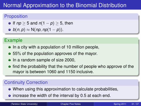
Normal Approximation to the Binomial Distribution
PropositionIf np ≥ 5 and n(1− p) ≥ 5, thenb(n,p) ≈ N(np,np(1− p)).
ExampleIn a city with a population of 10 million people,55% of the population approves of the mayor.In a random sample of size 2000,find the probability that the number of people who approve of themayor is between 1060 and 1150 inclusive.
Continuity CorrectionWhen using this approximation to calculate probabilities,increase the width of the interval by 0.5 at each end.
(Tarleton State University) Chapter Five Notes Spring 2011 31 / 37
ExampleSuppose X ∼ b(20,0.3).Approximate the following probabilities:
I P(2 ≤ X ≤ 8)I P(2 < X < 8)I P(2 < X ≤ 8)
(Tarleton State University) Chapter Five Notes Spring 2011 32 / 37
Normal Approximation to the Poisson Distribution
PropositionIf n is sufficiently large,then Poiss(n) ≈ N(n,n).
ExampleA radioactive sample emits β-particles according to a Poissonprocessat an average rate of 35 per minute.Find the probability that the number of particles emittedin a 20 minute period exceeds 720.
(Tarleton State University) Chapter Five Notes Spring 2011 33 / 37

Outline
1 Section 5.2: Transformations of Two Random Variables
2 Section 5.3: Several Independent Random Variables
3 Section 5.4: The Moment-Generating Function Technique
4 Section 5.5: Random Functions Associated with NormalDistributions
5 Section 5.6: The Central Limit Theorem
6 Section 5.7: Approximations for Discrete Distributions
7 Review for Exam 1
(Tarleton State University) Chapter Five Notes Spring 2011 34 / 37
Know how to do all homework and quiz problems.Given the joint p.d.f. of two random variables, be able to determine
I probabilities/expected values involving both random variables
P[(X ,Y ) ∈ A] =
∫ ∫A
f (x , y) dydx , for any A ⊂ R2.
E [u(X ,Y )] =
∫ ∞−∞
∫ ∞−∞
u(x , y)f (x , y) dydx .
I marginal p.d.f.’s and probabilities/expected values involving onlyone of the variables
f1(x) =
∫ ∞−∞
f (x , y) dy .
P(X ∈ A) =
∫A
f1(x) dx , for any A ⊆ R.
E [u(X )] =
∫ ∞−∞
u(x)f1(x) dx .
(Tarleton State University) Chapter Five Notes Spring 2011 35 / 37
I conditional p.d.f.’s, conditional mean/variance, and conditionalprobabilities
g(x | y) =f (x , y)
f2(y).
E [u(X ) | Y = y ] =
∫ ∞−∞
u(x)g(x | y) dx .
Var(X | Y = y) = E(X 2 | Y = y)− E(X | Y = y)2.
I the covariance and correlation coefficient
σXY = Cov(X ,Y ) = E(XY )− E(X )E(Y ).
ρ =Cov(X ,Y )
σXσY.
I the least squares regression line relating the variables
y = µY + ρσY
σX(x − µX ).
(Tarleton State University) Chapter Five Notes Spring 2011 36 / 37
Be able to find the expected value, variance, and probabilitiesinvolving Y , conditioning on X = x , when X and Y are jointlynormal
µY |x = E(Y | X = x) = µY + ρσY
σX(x − µX ).
σ2Y |x = Var(Y | X = x) = σ2
Y (1− ρ2).
The conditional distribution of Y given X = x is N(µY |x , σ2Y |x ).
Be able to find the distribution of Y = u(X ) using the distributionfunction technique or the change of variables formula.
G(y) = P(Y ≤ y) = P(u(X ) ≤ y), and g(y) = G′(y).
g(y) = f [v(y)]|v ′(y)|, where v = u−1.
g(y1, y2) = f [v1(y1, y2), v2(y1, y2)]
∣∣∣∣∣∣∣∣∣∣ ∂x1∂y1
∂x1∂y2
∂x2∂y1
∂x2∂y2
∣∣∣∣∣∣∣∣∣∣ .
Know the material in sections 5.3-5.6 and be able to solve relatedproblems.
(Tarleton State University) Chapter Five Notes Spring 2011 37 / 37
Top Related