


Languages
Pages
Legal


South Dakota State University South Dakota State University
Open PRAIRIE: Open Public Research Access Institutional Open PRAIRIE: Open Public Research Access Institutional
Repository and Information Exchange Repository and Information Exchange
Electronic Theses and Dissertations
2017
Price Discovery and Volatility Spillover Effects: The Agricultural Price Discovery and Volatility Spillover Effects: The Agricultural
ETPS and Their Underlying Commodities ETPS and Their Underlying Commodities
Yu Chen South Dakota State University
Follow this and additional works at: https://openprairie.sdstate.edu/etd
Part of the Economics Commons
Recommended Citation Recommended Citation Chen, Yu, "Price Discovery and Volatility Spillover Effects: The Agricultural ETPS and Their Underlying Commodities" (2017). Electronic Theses and Dissertations. 1142. https://openprairie.sdstate.edu/etd/1142
This Thesis - Open Access is brought to you for free and open access by Open PRAIRIE: Open Public Research Access Institutional Repository and Information Exchange. It has been accepted for inclusion in Electronic Theses and Dissertations by an authorized administrator of Open PRAIRIE: Open Public Research Access Institutional Repository and Information Exchange. For more information, please contact [email protected].
PRICE DISCOVERY AND VOLATILITY SPILLOVER EFFECTS: THE
AGRICULTURAL ETPS AND THEIR UNDERLYING COMMODITIES
BY
YU CHEN
A thesis submitted in partial fulfillment of the requirement for the degree
Master of Science
Major in Economics
South Dakota State University
2017


iii
ACKNOWLEDGEMENTS
I express my sincere gratitude to Dr. Zhiguang Wang as my advisor. Thanks for his
help in extending my knowledge on the investment and research, and improving my skills
and vision in this area, which benefits me greatly during my whole graduate life.
I would like to thank Dr. Lisa Elliott and Dr. Joseph Santos for their encouragement
and suggestions to my thesis and coursework. Your comments always can help me make
progress.
I would like to appreciate my fiancée, Shanshan Ma for supporting and encouraging
me in the completion of this thesis. Also I am very grateful to my friend, Justin Price,
Richard Mulder and Chad Te Slaa for their help with editing.

iv
TABLE OF CONTENTS
LIST OF FIGURES ........................................................................................................... vi
LIST OF TABLES ............................................................................................................ vii
ABSTRACT ..................................................................................................................... viii
CHAPTER 1 INTRODUCTION ........................................................................................ 1
1.1 Background ....................................................................................................................1
1.2 Problem Identification ...................................................................................................2
1.3 Research Objectives and Hypotheses ............................................................................5
1.4 Justification of the Study ...............................................................................................7
CHAPTER 2 LITERATURE REVIEW ............................................................................. 9
2.1 Price Discovery ..............................................................................................................9
2.2 Volatility Spillover.......................................................................................................15
CHAPTER 3 DATA AND METHODOLODY ............................................................... 21
3.1 Data Description ..........................................................................................................21
3.2 Tests of Stationarity and Cointegration .......................................................................24
3.3 Models..........................................................................................................................24
3.3.1 Vector Error Correction Model ..................................................................................... 25
3.3.2 Information Share ......................................................................................................... 27
3.3.3 Baba, Engle, Kraft, and Kroner model .......................................................................... 29
CHAPTER 4 RESULT ANALYSIS ................................................................................ 32
4.1 Summary Statistics.......................................................................................................32

v
4.2 Price Discovery between ETPs and Underlying ..........................................................37
4.2.1 Stationarity Test ............................................................................................................ 37
4.2.2 Cointegration Test ......................................................................................................... 39
4.2.3 Mean Equation (VEC model) ....................................................................................... 41
4.3 Information Share of ETPs and Underlying ................................................................48
4.4 Volatility Spillover between ETPs and Underlying.....................................................51
4.5 Magnitude of Volatility Spillovers between ETPs and Underlying ............................60
CHAPTER 5 CONCLUSIONS ........................................................................................ 62
REFERENCES ................................................................................................................. 66

vi
LIST OF FIGURES
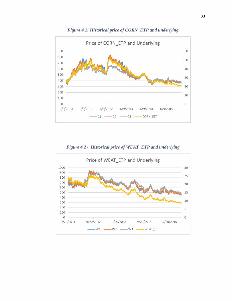
Figure 4.1: Historical price of CORN_ETP and underlying .......................................................... 33
Figure 4.2:Historical price of WEAT_ETP and underlying ....................................................... 33
Figure 4.3: Historical price of SOYB_ETP and underlying .......................................................... 34
Figure 4.4: Historical price of JJG_ETP and underlying ............................................................... 34
Figure 4.5: Historical price of DAG_ETP and underlying ............................................................ 35
Figure 4.6: Information share of ETPs throughout the history ...................................................... 51

vii
LIST OF TABLES
Table 4.1: Summary Statistics ....................................................................................................... 35
Table 4.2: Stationarity Test ............................................................................................................ 38
Table 4.3: Cointegration Test ........................................................................................................ 39
Table 4.4: VEC Model’s results of CORN_ETP and underlying .................................................. 44
Table 4.5: VEC Model's results of SOYB_ETP and underlying ................................................... 45
Table 4.6: VEC Model's results of WEAT_ETP and underlying .................................................. 45
Table 4.7: VEC Model's results of JJG_ETP and underlying ........................................................ 46
Table 4.8: VEC Model's results of DAG_ETP and underlying ..................................................... 47
Table 4.9: Estimates of information share of ETPs and underlying components .......................... 49
Table 4.10: BEKK Model's results of CORN_ETP and underlying .............................................. 56
Table 4.11: BEKK Model's results of SOYB_ETP and underlying .............................................. 56
Table 4.12: BEKK Model's results of WEAT_ETP and underlying ............................................. 57
Table 4.13: BEKK Model's results of JJG_ETP and Underlying .................................................. 58
Table 4.14: BEKK Model's results of DAG_ETP and Underlying .............................................. 59
Table 4.15: Magnitude of Volatility Spillover Effects between ETPs and Underlying ................. 61

viii
ABSTRACT
PRICE DISCOVERY AND VOLATILITY SPILLOVER EFFECTS: THE
AGRICULTURAL ETPS AND THEIR UNDERLYING COMMODITIES
YU CHEN
2017
This thesis investigates the price discovery and volatility spillover effects between
agricultural ETPs and commodity underlying. We analyze historical prices of five most
popular grain ETPs and their underlying commodities using VEC model and BEKK model.
Price discovery is confirmed by bidirectional relationships between ETPs and underlying
commodity in the long term, and the WEAT_ETP and CBOT Wheat Futures December
Contracts. In addition, findings show unidirectional relationships between ETPs and
underlying, mostly in the short term. In the process of price discovery, the information
share of ETPs is much lower than that of underlying, with a potential downward trend.
Volatility spillover is confirmed by bidirectional relationships between ETPs and
underlying, such as JJG_ETP and soybean futures, and confirmed by unidirectional
relationships, such as from wheat futures to DAG_ETP. For single commodity based ETPs,
the degree of volatility spillover from the nearby futures contracts to ETPs is higher than
that from distant futures contracts.

1
CHAPTER 1 INTRODUCTION
1.1 Background
Exchange Traded Products (ETPs) are a basket of securities, including stocks,
bonds, commodities, or indices. There are three types of ETPs, such as Exchange Traded
Funds (ETFs), Exchange Traded Notes (ETNs) and Exchange Traded Vehicles (ETVs).
The main benefits of investments in ETPs are found through the ease of diversification,
low expense ratios, tax efficiency, and transparency as well. This is combined with all the
standard trading structures of equities (e.g., options, short selling, stop losses, and limit
orders). ETPs can be bought and sold at any time during the trading day, in comparison to
mutual funds that can only be sold at the end of the day when their net asset value (NAV)
is calculated. Thus, in comparison to existing mutual funds or underlying securities, ETPs
tend to be an attractive investment tool.
In recent years, ETPs markets have been dramatically growing, not only in terms
of numbers and in terms of varieties of products, but also in terms of total assets and market
values. Initially, these products aimed at replicating broad-based stock indices. New ETPs
extended their fields to sectors, international markets, fixed-income instruments and lately
commodities. During the first half of 2015, globally listed exchange traded products (ETPs)
added $152 billion in net new assets, bringing total assets in the 11,295 listed funds to
$2.971 trillion, which is almost half of the passive mutual fund industry. This drastic
increase in value suggests that ETFs must have filled and continue to fill a gap in investors’
needs.

2
With increasing capitalization, ETPs have been playing a significant role in the
financial markets. However, it is the fact that ETPs are likely to be easily misused by
investors, which might lead to liquidity and volatility issues. This may rely on the fact that
ETPs are fairly new innovative financial products that a handful of investors, who are
trading ETPs, actually do not have a deep understanding of differences from other financial
derivatives in terms of investment strategies, complexities, latent risk, and regulations. For
example, ETFs like DIA, SPY, and QQQ, are the top three most actively traded securities
in the stock market. Due to clustering of volatility and the price discovery process, they are
found to have the price deviation that exists during trading days (DeFusco et al. 2007).
Also, in the futures market, price efficiency and volatility issues are a major concern after
introducing new ETPs to the market.
1.2 Problem Identification
In the secondary market, ETPs, a sized asset of around $2.91 trillion, have been a
considerable force that certainly impacts the movement of the whole market. Among ETPs,
ETFs are dominating trading in the market. Recent related research has been focusing on
three major topics: 1) exploring impacts of the arrival of ETFs on the underlying
components, 2) examining the efficiency of index derivatives markets, and 3) investigating
the price discovery of the index. Deville (2008) attempted to answer three major questions:
1) what impact does the advent of ETFs have on trading and market quality with regard to
index component stocks and index derivatives, 2) do ETFs represent a performing
alternative to conventional index funds, and 3) does the specific structure of ETFs allow
for more efficient index fund pricing?

3
With regard to ETPs’ impact on liquidity and volatility of securities, there is
currently no consensus in the literature. Empirical research has particularly found that
ETPs markets are likely to be more liquid and volatile than individual underlying securities,
and thus have strong potential impact on individual securities. On the other hand, other
research show that ETPs do not have a strong liquidity so that ETPs barely have interactive
impacts on component securities due to information asymmetry and the lack of arbitrage
opportunities in ETPs trading than individual stocks. (Park and Switzer 1995; Chou and
Kugele 2006; Madura and Richie 2005).
Looking with multiple views of the impact from ETPs, researchers draw attention
to price discovery and volatility spillover effects in order to have a deep understanding of
the advent of ETPs era. Price discovery which is interpreted as ‘the incorporation of the
information implicit in investor trading into market prices’ usually emphasizes the
existence of information share. The information share associated with a specific market is
defined as the proportion of the efficient price innovation variance that can be attributed to
that market. Information share is likely to cause tracking errors or price deviations. This
could explain why ETPs are traded at the premium or discount. Volatility spillover issues
investigate how volatility in one market is transferrable to other markets through the
arbitrage of goods between markets, which is usually distinguished temporarily, spatially,
and vertically.
Price discovery and volatility spillover could happen in the same market, but for
distinct securities, or for the same securities in different markets. For example, stocks in
the Dow Jones Industrial Average, which are tradable in many stock exchanges, have been
found to experience the existence of price discrepancy among different stock exchange

4
markets. Also, the phenomenon of price discovery and volatility spillover could appear
among related assets, but in a different market, such as commodity ETPs in the stock
market and their underlying components in the commodity futures market.
Originally, the arrival of commodity ETPs was designed to enhance the
diversification of the agricultural commodity index, and provide a more sophisticated
strategy for investing in commodities than were provided by conventional commodity
index. However, due to typical features such as cost saving, interest earned and
transparency, they have attracted a host of active and aggressive investors, which leads to
an increasing swing of liquidity among the futures market. Despite the importance of ETPs
to the commodity futures market, it currently still has limited research on the arrival of
agricultural ETPs. Thus far, research has found an existence of long-run co-integration
between ETN prices and the values of their underlying commodity indexes (Noman et al.
2013). However, research has not been done on that examine the price discovery process
and volatility spillover effect between commodity ETNs and their underlying.
It is interesting to note that the introduction of agricultural ETPs enriches investing
activities for commodity investors, by the fact that traders can continuously trade ETPs
instead of multiple commodity futures contracts, which includes a basket of commodity
future contracts in the secondary market throughout trading days. In this case, an important
question needs to be addressed: whether a volatile demand of ETPs will potentially lead to
price movement and volatility spillover to their underlying securities or vice versa (i.e., the
equity market vs. the commodity futures market)? In other words, it is reasonable to
question that whether high volume of ETPs’ trading would lead to high-frequency arbitrage
activity that can transfer the price pressure from the ETPs market to the underlying

5
securities, which results in the fact that the demand for ETPs would have a transmission
demand effect for the underlying securities. Conversely, it is also worth considering the
effect from underlying trading flows that would push a signal back to ETPs and probably
influence the demand of ETPs shares. Therefore, this study aims at discovering the price
discovery and volatility spillover effects between agricultural grain ETPs in the stock
market and their underlying commodities in the futures market.
1.3 Research Objectives and Hypotheses
Objective
This study is to investigate bidirectional price discovery and volatility spillover
effects between agricultural ETPs and their underlying commodities. In the first step, it is
necessary to understand how liquidity of commodity futures in the commodity market
could influence the liquidity of ETPs market, to uncover the existence of price discovery
between both markets, and eventually to quantify the contribution of the price discovery
from each market via the measure of information share. In the next step, if ETPs enables a
channel of arbitrage trading, it is worth investigating whether the introduction of ETPs
would cause volatility spillover effects among the ETP market and the markets of their
underlying components.
Hypotheses
1) There is a bilateral relationship in the price discovery of agricultural ETPs and
underlying, while the ETP market has a rising information share in the price
discovery of the underlying commodities.

6
Two important issues related to price discovery are (a) to determine which market
first incorporates new information about the underlying fundamental asset, and (b) how the
efficacy of price discovery depends on market liquidity and the prevalence of asymmetric
information. We use the information share (Hasbrouck 1995, Gonzalo and Granger 1995)
to measure each market’s contribution to the price discovery of the underlying
commodities. According to previous research, it has been seen an existence of information
share among indexes and their underlying. Therefore, in this study, we hypothesize that
there is a significant and increasing amount of information share arising from the newly
developed agricultural ETPs markets.
2) There is a bilateral volatility spillover effect between agricultural ETPs and
their underlying commodities.
Volatility spillovers would happen within multiple related markets because most
securities share common market information, have demand substitution effects on others,
and compete in the usage of some common inputs, such as production materials and labor.
When volatility in one market changes significantly, it leads to volatility movement in other
relative markets. Yang, Zhang, and Leatham (2003) found the evidence of volatility
transmission in the American and Canadian wheat market. Krause and Tse (2013)
uncovered the bi-directional volatility transmission among five comparable broad markets
and industry ETFs pairs in American and Canadian markets. Therefore, we hypothesize
that there is a bi-lateral volatility spillover effect existing between agricultural ETPs and
their underlying securities.

7
1.4 Justification of the Study
ETPs, typically index-based, consist of a basket of security assets. ETPs are
therefore created to track the investment performance of specific indices. In that case, there
is a theoretical relationship between ETPs and their underlying assets. This linkage is likely
to depend on a rational expectation hypothesis, through which, investors measure ETPs’
value as the net value of ETPs’ underlying assets. With the changing of the net value of
underlying securities, the value of ETPs fluctuate throughout the time. However, due to
asymmetric information and arbitrage activities existing in the market, it is hard to track
the net asset value of ETPs perfectly. Thus, to have a deep understanding of ETPs is
necessary.
Studies on price discovery and volatility spillover effects in the financial market
have shown multiple scenarios. They mostly focus on the relationships between liquid
securities and industry indexes. Some of them is to investigate the price discovery and
volatility transmission of same securities in different markets, while some is to uncover the
relationships for different securities in the same market. However, price discovery and
volatility transmission effects have rarely been studied among agricultural commodities
and agricultural indexes. To my best knowledge, there are some insights of the price
discovery between agricultural commodity futures and spot price. But I haven’t seen
quantified price discovery effects in the agriculture related paper, which will be applied in
the paper using Hasbrouck’s information share (1995). From that, we are able to capture
the proportional contributions of each single market in the process of price discovery.
From a policy perspective, it is vital to understand the impacts that ETPs have had
on the liquidity and volatility of commodity markets. If it is the case that ETPs are found

8
to have direct influence on the volatility of underlying securities, it may be necessary for
regulatory bodies to implement regulation to mitigate any potential effects. For example,
if it is found that ETFs are negatively impacting market functionality, then policy response
must focus on position limits, short-selling limits, and margin limits for ETFs.
This thesis is divided into five chapters. Chapter 1 describes the introduction,
research objectives and the justification of the study. Chapter 2 presents a review of
previous works related to price discovery and volatility spillover issues. Chapter 3
describes the data and research methodology used in the study. Chapter 4 presents and
analyzes the empirical results of the study. Chapter 5 concludes the study.

9
CHAPTER 2 LITERATURE REVIEW
This section reviews literature related to price discovery and volatility spillover
across multiple markets. With regard to the price discovery, it is divided into two sections.
The first section illustrates the price discovery in non-commodity markets, such as stock
index/ETPs and underlying stocks. The second section focuses on the price discovery
process related to the commodity market, such as commodity index/ETPs and commodity
futures. With regard to the volatility spillover, it includes two sections. The first section
involves volatility spillover effects between the agriculture commodity futures market and
the stock market. The second section illustrates previous studies of ETPs’ impact on
volatility.
2.1 Price Discovery
Price discovery in non-commodity markets
In general, price discovery is the process of determining an asset's full value
through a marketplace at a given time. Within the process, it refers to two definition of
values – observable price and unobservable price. The unobservable price reflects the
fundamental value of security assets. It is different from the observable price, which can
be broken down into its fundamental value and trading noise effects. Trading noise may
come from stochastic price movements due to factors such as bid-ask spreads swing,
inventory adjustments, and transient order imbalances.
Borkovec et al. (2010) conducted a study to discover linkages between exchange
traded funds and the broader market, and a potentially severe mismatch in liquidity. In an

10
attempt to answer the question on how does the liquidity provision affect price discovery
for exchange traded funds, Borkovec et al. investigated price discovery of ETFs in a
specific scenario: the U.S. financial markets on May 6th 2010. On this date, the market
experienced an abnormal incline, lasting only a few minutes before recovering. This event
is called a market flash crash. Their findings show that price discovery process failed for
ETFs during the flash crash, which proximately results from an extreme slack of liquidity,
both in ETFs and the relevant underlying components in the baskets. This might be a good
explanation why it is unrealistic to believe that the value of ETFs was to some extent re-
measured by market traders within a few minutes This resulted in a significant drop of
investors’ interest due to lack of depth, even though ETFs as a class of product have
attracted liquidity interest in other periods.
Hasbrouck (1995) investigated Dow Jones 30 stocks, which are tradable in many
stock exchanges, in order to discover price discrepancy and its mechanics among several
markets for same individual stocks. In other words, it is to explore that whether there exists
price discovery issues for one security that is trading in multiple markets. Hasbrouck adopts
a microstructure model to assess co-integration of individual stocks in different markets,
to determine how the information of stocks is transmitted among the different markets and
where the information share is dominant. Using the VAR model and VEC model,
Hasbrouck eventually shows that price discovery appears to be dominant in the NYSE
market, and the information share of most Dow stocks is larger than the NYSE's market
share (by trading volume).
Yan and Zivot (2002) summarized two types of price discovery measurements,
including the information share (IS) and the component share (CS) between multiple

11
markets. They adopted a structural cointegration model in order to clarify the application
of IS and CS. The model applies two types of structural price shocks: a permanent news
innovation to the common fundamental value, and a transitory liquidity/noise trading
shock. In the findings, Yan and Zivot showed that information share (IS) and the
component share (CS) are likely to be used together to distinguish the impacts of permanent
and transitory shocks to stocks. This is because neither IS nor CS alone can fully explain
the price discovery dynamics between multiple markets. In other words, the component
share cannot be interpreted as a market’s price responses to shocks, and the information
share failed to present the dynamics even when the cross-market innovations are
uncorrelated.
Henker & Marte (2006) attempted to contradict previous predictions that the futures
contract leads the index in the process of price discovery. They explored information share
between the security basket (HOLDR) and its portfolio (underlying components), and
eventually found out that the price of the portfolio of underlying securities is more
informative and leads the HOLDR (basket) price. This output is supportive of the
theoretical study by Subrahmanyam (1991), in which it is predicted that nonsynchronous
trading in the underlying components of an index may enlarge the probability of the lead
that the index net asset value surpasses its market price, and that the lead from the portfolio
to the basket is larger than that from the basket to the portfolio.
Due to the feature of intraday freedom-to-trade, ETPs’ prices are supposed to
fluctuate over the trading day, and its price will probably either be at a premium or discount
from the NAV. To clarify, if shares of an ETP trade at a discount below the net value of
the index’s underlying shares, the investor can long a host of ETP shares and short its

12
underlying components. In this case, price discrepancy of ETPs is hardly avoidable. Aber
et al. (2009) conducted a study on price volatility and tracking ability of ETFs, showing
that ETFs, when their daily prices appear to be volatile, have more possibility to trade at a
premium to their net asset value than at a discount, implying that the market tended to
overvalue these ETFs compared to their underlying NAVs. In addition, they stress that both
trading types have similar co-movement with their benchmarks, but are slightly
distinguished in terms of their tracking ability.
Due to regular management of ETPs, like formal creation and redemption, price
deviations are likely to appear. This is called a relative performance weakness by Gastineau
(2004). In the event of the mispricing of ETPs, investment arbitrage usually comes along
with price tracking errors. DeFusco et al. (2011) evaluated the pricing deviations of the
three most liquid ETFs, Spider, Diamonds and Cubes, from the price of the underlying
index by using the GARCH model. The conclusion was that the pricing deviation is
predictable due to its stationarity, series of volatility and lead-lag relationship. These
deviations are to be considered as additional costs for the ETFs.
In addition, Engle and Sarkar (2006) ever doubted that measurements of premiums
or discounts of ETFs in most models can be misleading because the net asset value of
ETFs’ underlying components is not correctly illustrated or because the price of ETFs is
inaccurately tracked. They attempted to introduce a new model, called the errors-in-
variables model. This model measures the standard deviation of the remaining pricing
errors and investigates the time variation in this standard deviation. Through the use of the
Kalman Filter State Space model, the ‘dyna’ model, and the GARCH model, Engle and
Sarkar eventually discover that the premiums (discounts) for the domestic ETFs, which is

13
typically slander and transitory, usually lasts only a few minutes. The standard deviation
of the premiums (discounts) is 15 basis points on average across all domestic ETFs, which
is considerably lower than the bid-ask spread. Meanwhile, premiums (discounts) of
international ETFs are much larger and last longer up to a few days. The reason for this
difference is explained by the higher cost and the complexity of the creation and
redemption of international ETFs. The bid-ask spreads are also much wider but are
comparable with the standard deviation of the premiums.
Price Discovery in Commodity Market
In the commodity futures market, price discovery is also a major issue. Agriculture
companies are highly involved in the process of producing and commercializing in which
information is generated and transferred into the market. In this process, it is not likely to
guarantee that information is appropriately interpreted and used, which to some extent
cause price deviation in the markets.
To improve our understanding of relative pricing efficiency on futures markets for
wheat, Yang and Leatham (1999) adopting the ECM, examined the dynamic-price
discovery mechanism in three wheat futures markets. The study states the prices of KCBT
were found to drive the price changes in both CBT and MGE in the long run. In the short
run, KCBT and CBT contributed more to the price information transmission for a longer
time while MGE was limited to a shorter time horizon. These findings were explainable by
the market microstructure of the three futures markets, including the role of underlying
cash wheat, market size, and speculation level.

14
Figuerola-Ferretti et al. (2010) demonstrated and measured the phenomenon of
price discovery in both futures markets and spot markets, adopting the two types of price
discovery processing created by Garbade and Silber (1983). These price discovery
processes combined with the method of permanent Transitory decomposition by Gonzalo
and Granger (1995), eventually illustrate an equilibrium model of price dynamics between
futures markets and spot markets with finite elasticity of arbitrage services and
convenience yields. Their findings demonstrate that the linear relationship in futures and
spot markets depends on the elasticity of arbitrage services and is determined by the
relative liquidity traded in the spot and futures markets. Also, after testing non-ferrous
metals prices (Al, Cu, Ni, Pb, Zn) traded in the London Metal Exchange (LME), Figuerola-
Ferretti et al. discovered backwardation is very common in most of the markets, and in
those highly liquid futures markets (Al, Cu, Ni, Zn), futures prices are typically information
dominant.
Storage is regarded as an economic force that connects the futures and cash market
in terms of commodity. Through storage, arbitrage might easily work. To explore the tie
of price discovery and commodity storage, Yang et al. (2002) examined the price discovery
performance of storable and non-storable commodities in the futures markets. Assuming a
perfect storable commodity model exists, which does not cause arbitrage, their findings
show that asset storability does not have a significant impact on the existing co-integration
between cash price and futures prices for agriculture commodities. Asset storability also
does not change the function of the futures market in predicting cash prices in the long run,
but it does, to some extent, impact the variance of futures markets’ prediction.

15
Index funds have been increasingly flowing into commodity futures markets over
the last decade, which, in principle, could have influence on the risk premium of the
commodity future contract through a large amount of buying. To have a deep
understanding of it, Hamilton and Wu (2013) attempted to look for a systematic
relationship between the expected returns of futures contracts and the net value of
commodity futures contracts held by index-fund traders using a simple regression model.
After testing 12 agricultural commodities, they found that it is not significant that the
investors’ positions of agricultural contracts possibly facilitate to predict returns on the
near futures contracts. In the oil futures market, their findings, under Singleton’s method,
showed some support of binary relation in the earlier data, especially in the recession of
2007-2009.
2.2 Volatility Spillover
Volatility spillover within Agriculture Markets
Volatility spillover is the idea that volatility in one market could transmit to other
markets, via sharing market information and the arbitrage of goods between markets. In
the financial market, many questions related to volatility spillover have often been asked
and investigated. Does the volatility of a major market lead to the volatility of other
markets? Does the volatility of an asset transmit or spillover to another asset directly or
indirectly through its conditional covariance? Do the innovations or the shocks from one
market increase the volatility in another market, and are the impacts the same for negative
and positive shocks?

16
Volatility spillovers exist among agricultural commodity markets because most
commodities share common market information, have demand substitution effects on
others, and compete in the usage of some common inputs, such as production materials and
labor. When volatility in one market changes significantly, it leads to volatility swings in
other relative markets. Such uncertainty and risks in the commodity market highly impact
production and marketing decisions for market participants.
In this case, research on volatility spillovers in agricultural commodity markets has
become an important issue. Researchers focus on an investigation of overall market
behaviors, and an exploration of the transmission of risks and shocks across interrelated
markets. To achieve such goals, it requires a recognition of linkages between different
markets and, in particular, the mechanism of volatility transmission among them. Also, the
dynamics of linkages are important indicators to help understand overall market behavior
and performance.
Yang, Zhang, and Leatham (2003), to discovery futures price and volatility
transmissions in the wheat market, conducted a study based on three wheat production
regions. These included the United States (US), Canada, and the European Union (EU).
Using a specific multivariate GARCH model (BEKK), their findings show that the
volatility of the EU market is self-dependent, but somehow has been able to transmit to the
U.S. and Canadian markets, but not vice versa. In addition, in the U.S., the volatility in
wheat prices is affected by Canadian markets, but not vice versa, which is interpreted as
Canada having the dominant role in the wheat market.
Buguk et al. (2003) conducted a study to examine whether the transmission of
volatility exists within a vertical catfish supply chain, knowing this phenomenon occurs in

17
the financial markets. They questioned whether price volatility in input markets (feeding
materials: corn, soybeans, menhaden) could transmit itself through higher market levels
(catfish feed and farm- and wholesale-level catfish), and vice versa. An exponential
GARCH (or EGARCH) model was used to capture possible spillovers among price series,
assuming a unidirectional transmission between feeding material and other market levels
according to the size of the catfish and feed markets relative to the corn and soybean
markets. In their results, they illustrate that there is a significant unidirectional spillover
between corn, soybean, menhaden prices, and catfish prices (feed, farm, and wholesale-
level fish prices), which provides evidence of volatility spillovers existing in an agricultural
market.
Zhao and Goodwin (2011), to investigate the topic of volatility spillovers, examined
relationships and transmissions among implied volatilities that are derived from two
options markets – corn and soybeans. They, using weekly average data from 2003 to 2010,
applied a VAR model with Fourier seasonal components as exogenous variables, impulse
response functions, and bootstrapped Chow tests. Their findings indicated that volatility
spillovers exist from the corn market to the soybean market, but not from the soybean
market to the corn market. In addition, from impulse response functions, they discovered
that responses of implied volatility in one market are positive and highly significant to a
shock in itself.
Du, Yu, and Hayes (2011) examined the roles of various factors influencing the
volatility of crude oil prices and the possible linkage between this volatility and agricultural
commodity markets (specifically corn and wheat). They applied a bivariate stochastic
volatility model to estimate three pairs of log returns of weekly crude oil, corn, and wheat

18
futures prices from November 1998 to January 2009. The model parameters are estimated
by the Bayesian Markov chain Monte Carlo methods. In their findings, Du, Yu, and Hayes
displayed evidence of volatility spillover among crude oil, corn, and wheat markets after
the fall of 2006. This could be largely explained by the tightened interdependent
relationships between markets, which is induced by ethanol production.
Serra and Gil (2012) studied the U.S. corn price fluctuations of the past two decades
to determine whether stock building can mitigate price fluctuations in a volatile food
market. They discovered that corn price volatility can be explained by the clustering
influence from energy prices, corn stocks, and the global economic conditions. A
multivariate GARCH specification that allows for exogenous variables in the conditional
covariance model is estimated both parametrically and semi parametrically. In the findings,
Serra and Gil showed that (1) there exists price volatility transmission between ethanol and
corn markets; (2) macroeconomic instability can increase corn price volatility; (3) stock
building is found to significantly reduce corn price fluctuations.
Volatility Spillover Related to ETPs market
The invention of ETPs is regarded as one of the most successful financial
innovations in the past twenty years. This kind of security portfolio gives the ability to
track the performance of the broad-base stock index. At the present, a handful of studies
are devoted to investigate the effects of ETPs arrival to the market. Researchers attempt to
answer a few questions: what impacts it has after introducing ETPs into the market and
how ETPs influence the liquidity of their underlying components? Among those topics,
most of them emphasize the examination of volatility effects from ETPs.
19
With ever increasing liquidity and arbitrage opportunities, ETFs have attracted a
handful of noise traders. This noise could be translated into underlying components through
the arbitrage channel, which contributes to the liquidity of underlying securities. Ben-
David et al. (2014) explored whether ETFs increase the non-fundamental volatility of the
underlying securities, using OLS regression and a regression discontinuity. Their output
displays that ETFs propagate to introduce new noise into the market, as opposed to
remodeling the existing noise, and stocks with higher ETF ownerships present substantially
higher volatility. More interestingly, they state that ETFs ownership presents a significant
relation with movement of component stock prices from a random walk at the intraday and
daily frequencies.
Krause and Tse (2013) conducted a study on how information flows across broad
market and industry ETFs in Canada and the United States, by examining the existence of
price discovery and volatility transmission among five comparable broad markets and
industry ETFs pairs in each market. Using the VAR model and EGARCH model, they
discover that volatility transmissions between the U.S. market and Canadian market are
highly bi-directional, while price discovery flows are consistently dominant from the U.S.
market to the Canadian market among ETFs. Also, information is captured more quickly
into prices through traded securities in the U.S. market, and the combination of negative
U.S. return spillovers and asymmetric volatility. This creates bilateral volatility spillover
effects.
Corbet and Twomey (2014) generated questions of whether commodity ETFs
amplify or influence volatility in the period after their introduction into international
commodity markets. In other words, does volatility effects from commodity ETFs act as

20
an accelerant for price deviation, or as a mechanism for liquidity improvements, thereby
expediting information transmission? Furthermore, given volatility effects exist
prominently, Corbet and Twomey continue to question whether the size of ownership of
the commodity among ETFs matters with effects. Using the EGARCH model, they found
out that larger market-proportional ETF holdings present higher volatility than smaller ETF
holdings, while smaller commodity markets, such as agriculture grain commodity, are
found to have growing liquidity flows, resulting from ETFs activities.
Lin and Chiang (2005) conducted a study to investigate volatility swings of
underling securities of the Taiwan 50 Index after the arrival of its ETF, named TTT.
Following a method that uses the unconditional variance of a GARCH model as the
volatility of underlying components of the Taiwan 50 Index, they demonstrated that the
volatility of the component stocks rise up after introducing TTT into the market. The
magnitude of volatility movement is not statistically distinguishable within most stock
sectors, but is in the electronic and the financial sector. In these sectors, the volatility of
TTT underlying companies increased dramatically after the advent of TTT. More
interestingly, it also displayed that the volatility of several companies in the mixed sector
are reduced to some extent.

21
CHAPTER 3 DATA AND METHODOLODY
3.1 Data Description
This study selects 5 typical ETPs of grain commodities with comparably higher
trading volumes, including Teucrium Corn Fund (CORN), Teucrium Soybean Fund
(SOYB), Teucrium Wheat Fund (WEAT), iPath Bloomberg Grains Subindex Total Return
ETN (JJG), PowerShares DB Agriculture Double Long ETN (DAG). Each ETP comprises
of several commodity futures underlying components, or tracking certain grain index
which comprises a basket of commodities futures.
The CORN’s net asset value (NAV) reflects the daily changes in percentage terms
of a weighted average of the closing settlement prices for three futures contracts of corn
commodity (“Corn Futures Contracts”) that are traded on the Chicago Board of Trade
(“CBOT”). Specifically, CORN comprises of three different Corn Futures Contracts: (1)
the second-to-expire CBOT Corn Futures Contract (C1), weighted 35%, (2) the third-to-
expire CBOT Corn Futures Contract (C2), weighted 30%, and (3) the CBOT Corn Futures
Contract expiring in the December following the expiration month of the third-to-expire
contract (C3), weighted 35%. (This weighted average of the three referenced Corn Futures
Contracts is referred to herein as the “Benchmark”.) Each contract is expected to roll over
in its last trading day.
Similarly, SOYB’s NAV is tracked by Soybean Futures Contracts Benchmark.
Specifically, the SOYB comprises of three different Soybean Futures Contracts: (1)
second-to-expire CBOT Soybean Futures Contract (S1), weighted 35%, (2) the third-to-
expire CBOT Soybean Futures Contract (S2), weighted 30%, and (3) the CBOT Soybean

22
Futures Contract expiring in the November following the expiration month of the third-to-
expire contract (S3), weighted 35%. Each contract is expected to roll over in its last trading
day.
Similarly, WEAT’s NAV is calculated by Wheat Futures Contracts Benchmark.
Specifically, the WEAT comprises of three different Wheat Futures Contracts: (1) the
second-to-expire CBOT Wheat Futures Contract (W1), weighted 35%, (2) the third-to-
expire CBOT Wheat Futures Contract (W2), weighted 30%, and (3) the CBOT Wheat
Futures Contract expiring in the December following the expiration month of the third-to-
expire contract (W3), weighted 35%. Each contract is expected to roll over in its last trading
day.
Additionally, JJG tracks the performance of Bloomberg Grains Subindex Total
ReturnSM (the “Grains ETNs”), which includes Corn Futures Contracts (42.71%), Soybean
Futures Contracts (32.49%), Chicago Wheat Futures Contracts (Cwheat) (18.24%), and
Kansas City Wheat Futures Contracts (Kwheat) (6.55%), whose weights are timely floating.
To minimize tracking errors, the Bloomberg Grains Subindex approaches a typical way for
rolling over commodity contracts, which counts on Lead Futures Contracts (front month
contracts) starting from 100% and reducing by 20% on each trading day, and Next Futures
Contracts (second month contracts), starting from 0% amount and rising by 20% on each
trading day, this process happens from 6th business day to 10th business day in each rolling
month.
Also, DAG tracks the performance of a total return version of the Deutsche Bank
Liquid Commodity Index – Optimum Yield Agriculture™ (the “Index”). The return on the
Index is derived by combining the returns on two component indices: the DB 3-Month T-

23
Bill Index (the “TBill index”) and the Deutsche Bank Liquid Commodity Index – Optimum
Yield Agriculture™ Excess Return (the “agriculture index”). The agriculture index is
intending to reflect the price changes, positive or negative, with a basket of four agricultural
commodities futures contracts: corn (weighted 25%), soybeans (weighted 25%), wheat
(weighted 25%), and sugar (weighted 25%). After the close of trading on February 16,
2012 (the "Effective Date"), one of underlying components in the agriculture index, wheat
futures contract, which was traded on the Board of Trade of the City of Chicago, Inc.
(“CBOT”), was replaced by a basket of three underlying futures contracts on wheat that
are traded on CBOT, the Kansas City Board of Trade (“KCBT”) and the Minneapolis Grain
Exchange, Inc. (“MGEX”), respectively. These contracts are weighted equally on each
rebalancing day, about 8.33% respectively. But to ensure the consensus of data, this study
still consider the factor of wheat futures contracts as previous as the CBOT wheat futures.
To avoid tracking error in the rolling month, the agriculture index approaches a typical
method to roll over each contract like Bloomberg Grains Subindex, adopting Lead Futures
Contracts and Next Futures Contracts changing with an amount of percentage, which starts
from 2nd business days to 6th business day in months prior to each contract expiration month.
In fact, the newly developed agricultural ETPs haven’t a long trading history. This
study will use all of their trading history by March 14th 2016, associated with their
underlying components. Among them, JJG has the longest trading history (October 23rd,
2007), then DAG (April 15th, 2008), CORN (June 8th, 2010), WEAT (September 19th,
2011), and SOYB (September 19th, 2011). Historical data of each ETP is obtained from
Yahoo Finance, while historical data of ETPs’ underlying is gained from Quandl Database.
To ensure the tracking accuracy, all the daily data of underlying securities are manipulated

24
according to the ETPs’ issuing prospects. To conduct this study, daily price of each
security is used.
3.2 Tests of Stationarity and Cointegration
If the stochastic data is non-stationary, the method of OLS would yield invalid
estimates, such as yielding high R square values and high t-ratios. This is called 'spurious
regression'. In order to prevent the disturbance of non-stationary data, it is necessary to test
the stationarity of the data sample in the beginning. Two methods are implemented to test
the stationarity of the data: the Augmented Dickey-Fuller (ADF) test and the Phillip and
Perron (PP) test. The ADF test is an augmented version of the Dickey–Fuller test for a
more complex time series models, allowing autocorrelation at higher order lags. The null
hypothesis of an ADF test is that there is a unit root in time series data samples. The Phillips
Perron test that builds on the Dickey–Fuller test of null hypothesis is helpful to test the unit
root among variables that has a high order of autocorrelation.
Then, the Johansen test, regarded as a multivariate generalization of the augmented
Dickey-Fuller test, is commonly used to test cointegrated relationships between variables.
The Johansen tests are likelihood-ratio tests that include maximum eigenvalue test and the
trace test. Because of this, the Johansen test permits to track more than one cointegrated
relationship when there are more than two variables.
3.3 Models
The main purpose of the research is to examine the existence of price discovery
between grain commodity ETPs and their underlying components which are trading in the
25
stock market and futures market, and to explore the volatility spillover effect among those
securities in different financial markets. To achieve this goal, this study will adopt the
Vector Error Correction Model (VECM) to discover the short-term and long-term
relationship between ETPs and their underlying. Based on that, this study then will apply
the mechanism of information share by Hasbrouck (1995), in order to quantify the value of
price discovery. Lastly, we will conduct the Baba, Engle, Kraft, and Kroner (BEKK) model
to examine shock and volatility transmission effects among them.
3.3.1 Vector Error Correction Model
Vector Error Correction Model (VECM) is commonly used with nonstationary
series that have a long-run stochastic trend, known as cointegration. To specify, the VECM
restricts the cointegrated relationships of the long-run behavior of the endogenous
variables, instead it captures a cointegration term that allows a wide range of short-run
dynamics. The cointegration term, known as the error correction term relates to last-periods
deviation from a long-run equilibrium, has influences on its short-run dynamics.
VECM is a representation of Vector Autoregression (VAR) Model, which assumes
that innovations are normally distributed. Firstly, we consider k variates and ith order vector
autoregressive time series,'
1, ,...t t k tY Y Y and VAR model as follow,
1 1 ...t t k t i tY C Y Y (1)

26
Where 1,2...,t n , and C is the constant term. The error term t is assumed to be k-
dimensional normally distributed (0, )N , where is the covariance matrix of the error
term. After introducing a k k matrix which defined as
1 ... k I (2)
We reformat VAR model as a VEC model,
1t t i t i tY C Y Y (3)
Or,
1, 1 1,1 11 1 11 1
, 1 ,1 1
. . . .
. .. . . . . . . . .
. .. . . . . . . . .
. . . .
t t it k k
t
k t k t ikt k kk k kk
Y YY
C
Y YY
(4)
Where1 2 3( , , ,... ) 'kC C C C C is a 1k vector of intercept terms,
1 ... k I is a
k k coefficient matrices, which illustrate the long run relationship,
1( ... ), 1,.. 1.i i p i p , is a k k coefficient matrices of t iY , which states the
short-term relationship,1 2 3( , , ,..., ) 't i t i t i t i kt iY Y Y Y Y is a 1k vector of
cointegrating factor, which t =1, t is a 1k vector of residuals.
From (3), this study investigates the significance of both long-run and shot-run
parameters to examine the price discovery effect of the mean returns between each
agricultural ETP and their underlying components. If coefficients related to ETPs in the
off-diagonal of the matrix are found to have a statistical significance, it means there are
price spillover effects existing between the ETP and its underlying components in the long
run. For example, if the model finds the significance of the ik parameters between an
underlying (i) and an ETP (k) for the sampled data, we can say price spillover effects are

27
found running from agricultural ETPs to underlying commodity in the long run, and vice
versa. Similarly, if coefficients related to ETPs in the off-diagonal of the matrix i are
found to have a statistical significance, it means there are price spillover effects existing
between the ETP and its underlying components in the short run. For example, if the model
finds the significance of theik parameters between an underlying (i) and an ETP (k) for
the sampled data, we can say price spillover effects is found running from agricultural
ETPs to underlying commodity in the short run, and vice versa. Meanwhile, the residual
t will be collected and used for analyzing volatility spillover effects by Baba, Engle, Kraft,
and Kroner model in the next step.
3.3.2 Information Share
Hasbrouck (1995) proposes a measurement for one market’s contribution to price
discovery based on the share of the variance of innovation that attributes to this market.
From the VEC model, Hasbrouck assumes that the “efficient price” of securities follows a
random walk and has the permanent component. Then, the information share decomposes
the variance of efficient price changes into components attributable to the different
markets. To compute the information share, the price changes are assumed to be covariance
stationary. This implies that they may be expressed as the vector moving average (VMA)
1 1 2 2t t t tY ... (5)
Wheret is a zero-mean vector of serially uncorrelated residual with the covariance matrix
, and i (i = 1, 2...p-1) coefficients are the impulse response parameters. The cumulative
impulse response function is

28
0
k
k i iM (6)
Where limk kM M . The rows of M are all identical. Let m be any row of M . So the
random-walk component of the prices is:
k tw m (7)
So the innovation variance is:
2 '
w m m (8)
If is diagonal, which means the market innovations are uncorrelated, then 'm m
will consist of k terms, each of which represents the contribution to the random-walk
innovation from a particular market. Then, the information share of the jth market is defined
as
2
'
j jj
j
mIS
m m
(9)
If is not diagonal, which means the market innovations are correlated, the
measurement of information share has the problem of attributing the covariance terms to
each market. To avoid this problem, Hasbrouck (1995) suggests to calculate the Cholesky
decomposition of and measure the information share using the orthogonalized
innovations. According to Hasbrouck (1995), the orthogonal innovation matrix contains
the upper and lower bounds, which are very close, generally within 0.001 of each other. To
be brief, this study only reports the lower bound in the analysis, since results using the
upper bound are virtually identical. Thus, Let F be a lower triangular matrix such that
'FF . Then the information share of the jth market is defined as

29
2
'
([ ] )j
j
mFIS
m m
(10)
Where [ ] jmF is the jth element of the row matrix mF .
The information share is a relative proportion of contribution that attributes to
different securities. It measures which security presents more informative values and
moves first in response to new information. For instance, if the information share of an
ETP is higher than that of its underlying components, we can say the ETP will move first
when responding to new innovation and there is more price discovery in the ETP, and vice
versa.
3.3.3 Baba, Engle, Kraft, and Kroner model
Baba, Engle, Kraft, and Kroner (BEKK) model, which is a class of Multivariate
GARCH model, is proposed by Engle and Kroner (1995) for investigating volatility
spillovers effects. The BEKK model allows for volatility spillover across multiple markets.
To achieve that goal, this method ensures the condition of a positive-definite conditional
variance-covariance matrix in the process of optimization.
In this study, the BEKK model is adopted to provide an appropriate path for
exploring the volatility transmission linkage between multiple securities that are trading in
different markets. In this model, we assume that variables have constant correlation and
innovations follow a Student's t distribution with v degrees of freedom. Below is a multi-
dimensional BEKK parameterization of our data series:
' ' '
1t tCC (11)

30
Where, t =
11, 1 ,
1, ,
. .
. . .
. . .
t k t
k t kk t
; C =
11 1
1
. .
. . .
. . .
. .
k
k kk
C C
C C
is an upper triangular matrix;
=
11 1
1
. .
. . .
. . .
. .
k
k kk
, is k k coefficient matrices; =
2
1, 1 1, 1 , 1
2
, 1 1, 1 , 1
. .
. . .
. . .
. .
t t k t
k t t k t
;
=
11 1
1
. .
. . .
. . .
. .
k
k kk
, is k k coefficient matrices; 1t =
11, 1 1 , 1
1, 1 , 1
. .
. . .
. . .
. .
t k t
k t kk t
;
Or,
211, 1 , 11 1 11 1 11 11, 1 1, 1 , 1
21, , 1 1 1, 1 1, 1 , 1
. . . . . . . .. .
. . . . . . . . . . . .. . .
. . . . . . . . . . . .. . .
. . . . . .. .
t k t k k kt t k t
k t kk t k kk k kk k kkk t t k t
C C
C C
11 1 11 111, 1 1 , 1
1 11, 1 , 1
. . . .. .
. . . . . .. . .
. . . . . .. . .
. . . .. .
k kt k t
k kk k kkk t kk t
(12)
In matrix A, the diagonal elements, depict the ARCH effect, measure the impact of
shocks on securities’ own volatility, and the off-diagonal elements illustrate spillover
effects from other securities’ shock. The coefficient ij (i=1, 2…k; j=1, 2...k ), given its
statistical significance, for example, presents a cross effect running from the lagged
residual terms of the security i to the security j and vice versa. In this study, each ETP is
placed in the last subsequence in each model. If the coefficient kj is related to an ETP, say
security k is an ETP and security j is an underlying for example, we could interpret that a
shock from the ETP has an important impact on the underlying, and vice versa.

31
In matrix B, the diagonal elements, depict the GARCH effect, measure each
security’s past volatility effect on its conditional variance, and the off-diagonal elements
captures the spillover effects from other securities’ the past volatility movement. The
coefficient ij (i=1, 2...k; j=1, 2...k), presents a cross-effect running from of the past
volatility movement of security i to the current volatility of security j, and vice versa. In
this study, each ETP is placed as the last variable in each model. If the coefficient kj is
related to an ETP, say security k is an ETP and security j is an underlying, we could
interpret that the past volatility movement from the ETP has an important spillover effect
on the volatility of underlying, and vice versa.
To measure the magnitude of volatility spillovers, the squared summation of the
cross terms of the BEKK model 2 2
ij ij (i=1, 2...k; j=1, 2...k) is adopted. If the
coefficients kj and kj are statistically significant, say security k is an ETP and security j
is an underlying, we can say the expression 2 2
kj kj measures the magnitude of volatility
spillover from the agricultural ETP (k) to the underlying (j), and vice versa. The difference
in magnitudes of volatility spillovers helps to identify the rank of contribution of volatility
from underlying to an ETP. And the difference in magnitudes of volatility spillovers helps
to identify the rank of contribution of volatility from an ETP to underlying. Due to the
different scales of price of ETPs and underlying, it is difficult to compare the magnitudes
of volatility spillovers from both sides. Therefore, in this study, we only aim to ranking the
contribution from one market to the other market.

32
CHAPTER 4 RESULT ANALYSIS
4.1 Summary Statistics
This paper examines the price discovery and volatility spillover effects between
grain commodity ETPs and their underlying components. To achieve this goal, this study
includes 5 ETPs. Some of them are specialized funds, which comprise a single type of
agricultural commodity futures, but different contract months, such as CORN, WEAT and
SOYB. Some are mixed funds, which comprise different types of agricultural commodity
futures, such as JJG and DAG. As the history of agricultural ETPs is not too long, this
study covers all of daily data for each fund since their inception dates. Specifically, CORN
and their underlying are starting from 06/08/2010-03/14/2016, WEAT and their underlying
are starting from 09/19/2011-03/14/2016, SOYB and their underlying are starting from
09/19/2011-03/14/2016, JJG and their underlying are starting from 10/23/2007-03/14/2016,
and DAG and their underlying are starting from 04/15/2008-03/14/2016. Figure 4.1 graphs
historical price of CORN_ETP and its underlying, C1, C2 and C3. Figure 4.2 graphs
historical price of WEAT_ETP and its underlying, W1, W2 and W3. Figure 4.3 graphs
historical price of SOYB_ETP and its underlying, S1, S2 and S3. Figure 4.4 graphs
historical price of JJG_ETP and its underlying, corn futures, soybean futures, Cwheat
futures and Kwheat futures. Figure 4.5 graphs historical price of DAG_ETP and its
underlying, corn futures, wheat futures, soybean futures and sugar futures. The price
history of selected ETPs and their underlying is shown in Figures 4.1-4.5. Descriptive
summary of historical price data is reported in Table 4.1.
33
Figure 4.1: Historical price of CORN_ETP and underlying
Figure 4.2:Historical price of WEAT_ETP and underlying

34
Figure 4.3: Historical price of SOYB_ETP and underlying
Figure 4.4: Historical price of JJG_ETP and underlying

35
Figure 4.5: Historical price of DAG_ETP and underlying
Figures 4.1 – 4.5 show historical price data of ETPs along with commodity
underlying. As we can see, the price of CORN_ETP, SOYB_ETP and WEAT_ETP along
with underlying started low and suddenly peaked in the year of 2012, then followed by a
gradual slump. The price of JJG_ETP and DAG_ETP along with commodity underlying
started high in mid-2008 and ended low by 2016 after experiencing fluctuated years. This
fluctuation of grain commodity market might result from several economic and non-
economic issues, such as the 2007-2008 financial crisis and the 2012-2013 drought. In
addition, roughly speaking, these graphs indicate the movement of ETPs go consistently
with their underlying throughout the period.
Table 4.1: Summary Statistics
Table 4.1 presents summary statistics of five ETPs and their underlying
components. C1, C2 and C3 represent the second-to-expire CBOT Corn Futures Contract,

36
the third-to-expire CBOT Corn Futures Contract and the CBOT Corn Futures Contract
expiring in the December following the expiration month of the third-to-expire contract.
Similarly, S1, S2 and S3 represent soybean futures contracts, and W1, W2 and W3
represent wheat futures contracts. The sample data are from different time ranges.
Specifically, CORN and their underlying are in 06/08/2010-03/14/2016 WEAT and their
underlying are in 09/19/2011-03/14/2016, SOYB and their underlying are in 09/19/2011-
03/14/2016, JJG and their underlying are in 10/23/2007-03/14/2016, and DAG and their
underlying are in 04/15/2008-03/14/2016. St. Dev stands for “standard deviation.”
In Table 4.1, observations of sample data are diverse, due to different inception
dates. The big gap between minimum and maximum price of each security indicates the
grain ETPs and commodity underlying have been through a volatile period. Speaking of
the skewness, it is to measure the asymmetry of the probability distribution of a random
variable. Most of estimates of skewness are moderate positive, within the range of -1 to 1,
Table 4.1
Variables Obs. Mean St.Dev. Median Min Max Skewness Kurtosis
C1 1437 534.648 141.537 507.500 333.250 838.750 0.269 -1.378
C2 1437 531.832 133.265 506.750 342.000 837.750 0.371 -1.208
C3 1437 505.415 86.795 505.500 366.750 681.500 0.139 -1.308
CORN_ETP 1437 34.812 8.702 35.120 20.535 52.670 0.036 -1.247
W1 1117 634.321 117.184 638.000 446.000 948.250 0.635 -0.176
W2 1117 644.017 116.871 651.250 452.500 936.500 0.559 -0.275
W3 1117 667.587 106.502 680.000 477.500 910.000 0.198 -0.783
WEAT_ETP 1117 16.180 4.930 16.290 8.560 25.350 0.133 -1.295
S1 1121 1225.795 232.237 1272.000 855.250 1768.250 -0.040 -1.100
S2 1121 1207.092 217.536 1257.750 855.500 1766.250 0.043 -0.874
S3 1121 1136.369 160.109 1176.500 859.750 1552.500 -0.214 -1.130
SOYB_ETP 1121 22.259 2.690 22.830 17.060 28.850 -0.226 -0.755
CORN 2157 500.012 142.728 441.000 293.500 831.250 0.550 -1.152
SOYBEAN 2157 1195.262 225.623 1205.000 783.500 1771.000 0.190 -1.100
CWHEAT 2157 638.508 142.151 624.500 428.000 1280.000 0.843 0.564
KWHAET 2157 681.148 157.309 680.750 430.760 1337.000 0.519 -0.076
JJG_ETP 2157 45.025 9.652 44.620 29.480 74.430 0.528 -0.388
CORN 1914 502.758 145.353 438.250 293.500 831.250 0.523 -1.227
WHEAT 1914 666.240 138.043 676.000 453.500 1051.500 0.319 -0.925
SOYBEAN 1914 1194.027 228.851 1199.250 781.750 1771.000 0.192 -1.138
SUGAR 1914 18.599 5.361 17.320 9.530 35.310 0.734 -0.207
DAG_ETP 1914 9.514 4.369 9.175 2.940 28.780 1.112 2.329

37
which means the bulk of the data lies to the right of the mean. This implies that the price
of commodity is tending to rise up. Few variables, such as S1, S3 and SOYB_ETP, show
negative skewness in price, which means that the majority of the data lies to the left of the
mean, Furthermore, kurtosis is a measure of the ‘peakedness’ of the probability distribution
of a random variable, which describes the shape of a probability distribution. Most
estimates of kurtosis are slightly negative, which displays platykurtic shapes with an acute
tails and a fatter peak around the mean for the sampled period. Since all the estimates are
within the range from -3 to 3, they are all acceptable. Compared to kurtosis values of each
underlying, DAG_ETP’s and WEAT_ETP’s are fairly higher, which indicates that the data
tends to have light peak, or outliers.
4.2 Price Discovery between ETPs and Underlying
4.2.1 Stationarity Test
Two methods are implemented to test the existence of stationarity of the date: The
Augmented Dickey-Fuller (ADF) test and the Phillip and Perron (PP) test. The ADF test is
an augmented version of the Dickey–Fuller test for a more complex time series model,
allowing autocorrelation at higher order lags. The null hypothesis of an ADF test is that
there is a unit root present in a time series sample. The Phillips Perron test that builds on
the Dickey–Fuller test of the null hypothesis is helpful to test the unit root in the data that
has a high order of autocorrelation.

38
Table 2: Stationarity Test
Table 4.2 reports the results of unit root tests (Augmented Dickey-Fuller and
Phillips-Perron). C1, C2 and C3 represent the second-to-expire CBOT Corn Futures
Contract, the third-to-expire CBOT Corn Futures Contract and the CBOT Corn Futures
Contract expiring in the December following the expiration month of the third-to-expire
contract. Similarly, S1, S2 and S3 represent soybean futures contracts, and W1, W2 and
W3 represent wheat futures contracts.
Table 4.2 presents two types of stationarity test: ADF test and PP test. All the tests
show lack of statistical significance against the null hypothesis of unit root or non-
Table 4.2
Security Decision
Statistics P Value Alpha P Value
C1 -1.418 0.531 -12.190 0.429 Fail to Reject
C2 -1.454 0.517 -12.657 0.404 Fail to Reject
C3 -1.535 0.487 -13.312 0.367 Fail to Reject
CORN_ETP -1.046 0.670 -10.124 0.545 Fail to Reject
S1 -0.847 -0.847 -7.504 0.691 Fail to Reject
S2 -0.961 0.744 -9.134 0.600 Fail to Reject
S3 -1.286 0.580 -18.684 0.091 Fail to Reject
SOYB_ETP -1.580 0.470 -9.852 0.560 Fail to Reject
W1 -1.295 0.577 -10.583 0.519 Fail to Reject
W2 -1.226 0.602 -10.447 0.527 Fail to Reject
W3 -1.257 0.591 -12.521 0.411 Fail to Reject
WEAT_ETP -1.182 -1.182 -15.234 0.260 Fail to Reject
CORN -1.819 0.3807 -7.399 0.697 Fail to Reject
SOYBEAN -2.444 0.1472 -10.169 0.5425 Fail to Reject
CWHEAT -2.621 0.0915 -14.381 0.3076 Fail to Reject
KWHAET -2.120 0.2684 -11.593 0.4631 Fail to Reject
JJG_ETP -1.887 0.3554 -9.8221 0.5619 Fail to Reject
CORN -1.862 0.3646 -6.754 0.733 Fail to Reject
WHEAT -2.790 0.06332 -12.729 0.3998 Fail to Reject
SOYBEAN -2.359 0.179 -8.7977 0.619 Fail to Reject
SUGAR -2.071 0.2867 -8.9835 0.6087 Fail to Reject
DAG_ETP -3.521 0.01 -18.016 0.1048 Fail to Reject
ADF Test PP Test

39
stationarity, so that fail to reject the null hypothesis. Thus, it concludes that the price data
of securities are non-stationary. Next, the cointegration test is described below.
4.2.2 Cointegration Test
Johansen (1988) develops maximum likelihood estimators of cointegrating vectors
and provides a rank test to determine the number of cointegrating vectors, r. In this study,
the Johansen test has been used to investigate the cointegrated relationship between each
ETP and commodity underlying, includes two types of tests maximal trace test and
maximal eigenvalue test. In this study, we adopt maximal eigenvalue test as an indicator,
testing the null hypothesis that there are (at most) r (0 < r < p) cointegrated vectors. To be
accurate, this study proposes an assumption during the test: whether there is a linear trend
existing in the model.
Table 4.3: Cointegration Test
Table 4.3 presents summary of cointegration test for each ETP and underlying. C1,
C2 and C3 represent the second-to-expire CBOT Corn Futures Contract, the third-to-expire
CBOT Corn Futures Contract and the CBOT Corn Futures Contract expiring in the
December following the expiration month of the third-to-expire contract. Similarly, S1, S2
and S3 represent soybean futures contracts, and W1, W2 and W3 represent wheat futures
contracts. Cwheat and Kwheat represent nearby Chicago Wheat Futures Contract and
Kansas Wheat Futures Contract respectively. All tests adopt maximal eigenvalue statistic
under two types of methods: without/with linear trend. Within the result, 'r' means the
number of cointegrated relationship, and 'test' means values of test statistic. All the tests
reject the hypothesis, which imply the existence of cointegration.

40
Table 4.3 displays results of the cointegration test for each ETP and its underlying.
Taking CORN_ETP and its underlying components for example. When the finding of the
hypothesis of r<=0 and r<=1 is much larger than 5% critical value, it presents the
hypothesis is rejected, which means there are at least two cointegration among CORN_ETP,
C1,C2 and C3 (i.e., the intercepts in the long-run relations). Similarly, tests for
WEAT_ETP and SOYB_ETP and their underlying have all been witnessed to reject the
hypothesis of r<=0 at 5% critical value, resulting in the evidences of at least one
cointegrated relationships among them respectively. Also, the test of JJG_ETP rejects the
Table 4.3
Securities
H0=r Test 5% Critical Value Test 5% Critical Value
C1 r=0 37.31 28.14 37.57 31.46
C2 r<=1 31.98 22.00 32.77 25.54
C3 r<=2 7.69 15.67 7.65 18.96
CORN_ETP r<=3 3.62 9.24 4.50 12.25
S1 r=0 31.40 28.14 45.52 31.46
S2 r<=1 15.42 22.00 15.50 25.54
S3 r<=2 10.97 15.67 13.78 18.96
SOYB_ETP r<=3 4.83 9.24 8.78 12.25
W1 r=0 37.52 28.14 37.99 31.46
W2 r<=1 15.58 22.00 18.70 25.54
W3 r<=2 10.37 15.67 12.06 18.96
WEAT_ETP r<=3 4.76 9.24 4.75 12.25
CORN r=0 43.16 34.40 44.89 37.52
SOYBEAN r<=1 20.40 28.14 24.70 31.46
K.WHEAT r<=2 15.87 22.00 16.86 25.54
C.WHEAT r<=3 6.11 15.67 7.17 18.96
JJG_ETP r<=4 3.77 9.24 4.15 12.25
CORN r=0 541.55 34.40 523.09 37.52
SOYBEAN r<=1 37.71 28.14 47.10 31.46
WHEAT r<=2 20.72 22.00 27.69 25.54
SUGAR r<=3 14.87 18.96 14.93 18.96
DAG_ETP r<=4 4.54 9.24 6.14 12.25
Without linear trend With linear trend

41
hypothesis of r<=1 at 5% critical value, which shows at least two cointegrated relationship
existing among JJG_ETP, corn futures, soybean futures, Kwheat futures and Cwheat
futures. Besides, the test of DAG_ETP rejects the hypothesis of r<=0 and r<=1 at 5%
critical value, which illustrates multiple cointegration existing between DAG_ETP, corn
futures, soybean futures, wheat futures and sugar futures. Therefore, it concludes that failed
rejections of the null hypothesis imply that there exists at least two co-integrating vector
which confirms a long run equilibrium relationship between the each agricultural ETP and
underlying.
4.2.3 Mean Equation (VEC model)
From the test of cointegration, it shows the evidence of cointegration between
variables, which suggests a long term relationship between variables. To avoid the noise
of cointegration, the VEC model is necessary to be applied. The VEC model allows the
long run behavior of the endogenous variables to converge to their long run equilibrium
relationship while allowing a wide range of short run dynamics.
Tables 4.4-4.8 report results of VEC models of five ETPs, CORN_ETP,
WEAT_ETP, SOBY_ETP, JJG_ETP, DAG_ETP and their underlying. With regard to
CORN_ETP, the long run equilibrium relationships from CORN_ETPt-1 to ∆C2t and ∆C3t
are confirmed, which are statistically significant at 1% and 10% level respectively. Yet,
there is no evidence of long run relationships from underlying to ∆CORN_ETPt. This
means the impact of the CORN_ ETP’s price movement, in the long run, can be transmitted
to its underlying, especially C1 and C2, and not vice versa. Furthermore, the short run
price transmissions from ∆CORN_ETPt-1 to ∆C1t, ∆C2t and ∆C3t are obtained, which

42
shows 1%, 1% and 10% statistical significance level respectively, and not vice versa. This
means impacts from the CORN_ETP is significant to the price movement of C1, C2 and
C3 in the short run. Overall, there is a unilateral relationship from the CORN_ETP to C2
and C3 in the long run, while there are unilateral relationships from the CORN_ETP to its
underlying in the short run, C1 and C2 in particularly.
With regard to SOYB_ETP, the long run equilibrium relationships from
SOYB_ETPt-1 to ∆S1t, ∆S2t and ∆S3t are confirmed, which are statistically significant at
1%, 1% and 5% level respectively. And, there also exists a long run relationship from S1t-
1 to ∆SOYB_ETPt, at 5% significance level. This means, in the long run, the impact of the
SOYB_ ETP’s price movement can be transmitted to all of its underlying, while the impact
of S1 can be transmitted to SOYB_ ETP. Furthermore, the short run price transmissions
from ∆S2t-1 and ∆S3t-1 to ∆SOYB_ETPt are observed, which shows 5% and 5% statistical
significance level respectively, and not vice versa. This means impacts from the S2 and S3
are significant to the price movement of SOYB_ ETP in the short run. Overall, in the long
run, there are unilateral relationships from the SOYB_ETP to S2 and S3 and a bilateral
relationship between SOYB_ETP and S1, while there are unilateral relationships from S2
and S3 to SOYB_ETP in the short run.
With regard to WEAT_ETP, the long run equilibrium relationships from
WEAT_ETPt-1 to∆W1t and ∆W3t are confirmed, which are statistically significant at 5%
and 5% level respectively. And, there also exist long run relationships from W2t-1 and W3t-
1 to ∆WEAT_ETPt, at 10% and 5% significance level respectively. This means, in the long
run, the impact of the WEAT_ETP’s price movement can be transmitted to its underlying,
such as W1 and W3, while the price impact of W2 and W3 can be transmitted to WEAT_

43
ETP. Furthermore, there is no evidence that shows a unilateral or bilateral relationship
between the WEAT_ETP and its underlying in the short run, since none of their coefficients
is statistically significant. Overall, there, in the long run, are a unilateral relationship from
the WEAT_ETP to W1 and a unilateral relationship from W2 to WEAT_ETP, as well as a
bilateral relationship between WEAT_ETP and W3, while there is no evidence of
equilibrium relationships between WEAT_ETP and the underlying in the short run.
Regarding to the JJG_ETP, the long run equilibrium relationships from JJG_ETPt-
1 to ∆CORNt and ∆KWHEATt are confirmed, which are statistically significant at 1% and
5% level respectively, while there is no relationship observed from underlying to the
JJG_ETP. This means, in the long run, the impact of the JJG_ETP’s price movement can
be transmitted to its underlying, such as CORN and KWHEAT, and not vice versa.
Furthermore, the short run price transmission from ∆JJG_ETPt-1 to ∆SOYBEANt,
∆CWHEATt and ∆KWHEATt are observed, which shows 1%, 10% and 1% statistical
significance level respectively, and not vice versa. Overall, in the long run, there are
unilateral relationships from JJG_ETP to corn futures and Kansas wheat futures, while
there are strong unilateral relationships from JJG_ETP to soybean futures and Kansas
wheat futures in the short run.
In regards to DAG_ETP, the long run equilibrium relationships from DAG_ETPt-1
to ∆SOYBEANt , ∆WHEATt , and ∆SUGARt are confirmed, which are statistically
significant at 10%, 10% and 10% level respectively, while only a long relationship from
CORNt-1 to ∆DAG_ETPt is observed too at 1% significance level. This means, in the long
run, the impact of the CORN’s price movement can be transmitted to DAG_ETP, while
DAG_ETP has a slight impact on its underlying, such as SOYBEAN, WHEAT and

44
SUGAR. Furthermore, the short run price transmission from ∆CORNt-1, ∆WHEATt-1 and
∆SUGARt-1 to ∆DAG_ETPt are observed, which shows 5%, 5% and 10% statistical
significance level respectively, and not vice versa. Overall, there is, in the long run, a
unilateral relationship from corn futures to DAG_ETP, while there are unilateral
relationships from corn futures and wheat futures to DAG_ETP in the short run.
Table 4.4: VEC Model’s results of CORN_ETP and underlying
Table 4.4 presents the output of VEC model about the CORN_ETP and its
underlying. C1, C2 and C3 represent the second-to-expire CBOT Corn Futures Contract,
the third-to-expire CBOT Corn Futures Contract and the CBOT Corn Futures Contract
expiring in the December following the expiration month of the third-to-expire contract.
Values without parentheses are estimated parameters, values below parameter estimates
are p-values. Note, ***, ** and * denote statistical significance at 1%, 5% and 10% levels,
respectively.
Table 4.4
∆CORN_ETPt ∆C1t ∆C2t ∆C3t
CORN_ETPt-1 0.005 0.166 0.530 0.265
0.646 0.41 0.00 *** 0.06*
C1t-1 0.000 -0.034 -1.326 0.008
0.880 0.016** 0.174 0.407
C2t-1 0.001 0.039 -1.027 0.005
0.503 0.005*** 0.00 *** 0.616
C3t-1 -0.002 -0.035 -0.461 -0.058
0.067* 0.110 0.00 *** 0.00 ***
∆CORN_ETPt-1 -0.085 5.784 3.751 1.722
0.237 0.00 *** 0.001*** 0.062*
∆C1t-1 -0.001 -0.149 -0.105 -0.070
0.891 0.021** 0.100 0.135
∆C2t-1 -0.004 0.027 0.024 0.014
0.234 0.686 0.71 0.773
∆C3t-1 -0.004 -0.274 -0.212 -0.121
0.324 0.001*** 0.014** 0.05*

45
Table 4.5: VEC Model's results of SOYB_ETP and underlying
Table 4.5 presents the output of VEC model about the SOYB_ETP and its
underlying.
S1, S2 and S3 represent the second-to-expire CBOT Soybean Futures Contract, the third-
to-expire CBOT Soybean Futures Contract and the CBOT Soybean Futures Contract
expiring in the December following the expiration month of the third-to-expire contract.
Values without parentheses are estimated parameters, values below parameter estimates
are p-values. ***, ** and * denote statistical significance at 1%, 5% and 10% levels,
respectively.
Table 4.6: VEC Model's results of WEAT_ETP and underlying
Table 4.6 presents the output of VEC model about the WEAT_ETP and its
underlying. W1, W2 and W3 represent the second-to-expire CBOT Wheat Futures Contract,
the third-to-expire CBOT Wheat Futures Contract and the CBOT Wheat Futures Contract
expiring in the December following the expiration month of the third-to-expire contract.
Values without parentheses are estimated parameters, values below parameter estimates
are p-values. Note, ***, ** and * denote statistical significance at 1%, 5% and 10% levels,
respectively.
Table 4.5
∆SOYB_ETPt ∆S1t ∆S2t ∆S3t
SOYB_ETPt-1 -0.050 -1.747 -1.736 -1.692
0.00 *** 0.033** 0.030** 0.001***
S1t-1 0.001 -0.015 0.013 0.057
0.023* 0.522 0.560 0.002
S2t-1 -0.002 0.029 -0.001 -0.024
0.443 0.164 0.970 0.149
S3t-1 0.000 0.008 0.001 -0.045
0.644 0.628 0.935 0.00***
∆SOYB_ETPt-1 -0.458 -2.058 -1.192 -0.010
0.00 *** 0.475 0.672 0.775
∆S1t-1 0.001 0.061 -0.012 -0.036
0.367 0.518 0.896 0.636
∆S2t-1 0.003 -0.014 -0.033 -0.016
0.043** 0.888 0.739 0.840
∆S3t-1 0.002 -0.044 -0.025 -0.003
0.036** 0.464 0.669 0.946

46
Table 4.7: VEC Model's results of JJG_ETP and underlying
Table 4.7 presents the output of VEC model about the JJG_ETP and its underlying.
CORN represent the nearby CBOT Corn Futures Contract. Similarly, SOYBEAN,
CWHEAT represent the nearby CBOT Soybean Futures Contract. KWHEAT represent
nearby Kansas Wheat Futures Contract. Values without parentheses are estimated
parameters, values below parameter estimates are p-values. Note, ***, ** and * denote
statistical significance at 1%, 5% and 10% levels, respectively.
Table 4.6
∆WEAT_ETPt ∆W1t ∆W2t ∆W3t
WEAT_ETPt-1 -0.057 -1.532 -1.818 -1.246
0.00 *** 0.014** 0.386 0.026**
W1t-1 -0.002 -0.141 -0.073 -0.073
0.229 0.089* 0.356 0.323
W2t-1 0.005 0.214 0.136 0.148
0.062* 0.036** 0.165 0.105
W3t-1 -0.002 -0.062 0.053 -0.070
0.014** 0.017** 0.033** 0.002***
∆WEAT_ETPt-1 -0.464 -2.107 -1.818 -0.715
0.00 *** 0.337 0.386 0.715
∆W1t-1 0.008 0.309 0.334 0.125
0.142 0.173 0.123 0.535
∆W2t-1 0.004 -0.195 -0.249 -0.060
0.609 0.496 0.364 0.814
∆W3t-1 -0.001 -0.103 -0.072 -0.097
0.751 0.309 0.459 0.282

47
Table 4.8: VEC Model's results of DAG_ETP and underlying
Table 4.8 presents the output of VEC model about the DAG_ETP and its underlying.
CORN represent the nearby CBOT Corn Futures Contract. Similarly, SOYBEAN,
CWHEAT represent the nearby CBOT Soybean Futures Contract. KWHEAT represent
nearby Kansas Wheat Futures Contract. Values without parentheses are estimated
parameters, values below parameter estimates are p-values. Note, ***, ** and * denote
statistical significance at 1%, 5% and 10% levels, respectively.
Table 4.7
∆JJG_ETPt ∆CORNt ∆SOYBEANt ∆CWHEATt ∆KWHEATt
JJG_ETPt-1 -0.023 -0.321 -0.029 0.013 0.331
0.018** 0.009*** 0.913 0.944 0.003**
CORNt-1 0.000 -0.002 0.014 -0.001 -0.079
0.535 0.503 0.034* 0.859 0.157
SOYBEANt-1 0.000 0.002 -0.017 0.004 -0.128
0.448 0.459 0.006*** 0.315 0.015*
CWHEATt-1 0.001 0.012 0.013 -0.009 -0.175
0.129 0.165 0.488 0.504 0.048 *
KWHEATt-1 0.000 0.005 -0.001 -0.003 -0.939
0.774 0.493 0.934 0.916 0.001 **
∆JJG_ETPt-1 -0.012 0.042 6.967 2.144 2.747
0.125 0.955 0.00 *** 0.053* 0.00***
∆CORNt-1 -0.001 0.034 -0.256 -0.134 -0.158
0.726 0.338 0.00 *** 0.012** 0.002***
∆SOYBEANt-1 0.002 0.049 -0.112 -0.012 -0.055
0.115 0.001*** 0.00 *** 0.543 0.117
∆CWHEATt-1 -0.006 -0.082 -0.160 -0.181 -0.147
0.079* 0.085* 0.245 0.043** 0.007***
∆KWHEATt-1 0.004 0.039 0.039 0.136 0.180
0.125 0.413 0.703 0.055* 0.007***

48
4.3 Information Share of ETPs and Underlying
A market's contribution to price discovery is the "information share". According to
Hasbrouck (1995), information share measures the market's contribution to which is the
proportion of the efficient price innovation variance that can be attributed to that market.
This efficient price is unobservable, but common to all the markets. Intuitively, information
share proxies for 'who moves first' in the price discovery.
Table 4.9 reports information share is allocated differently in ETPs and underlying
components. Taking CORN_ETP and its underlying for example. The information share
of C1 counts much more than C2, C3 and CORN_ETP, about 0.803, while that of
Table 4.8
∆DAG_ETPt ∆CORNt ∆SOYBEANt ∆WHEATt ∆SUGARt
DAG_ETPt-1 -0.225 -0.281 0.612 -0.340 -0.014
0.00 *** 0.115 0.083* 0.073* 0.053*
CORNt-1 0.000 -0.010 0.012 0.009 0.000
0.004** 0.528 0.226 0.092* 0.923
SOYBEANt-1 0.000 -0.003 -0.018 0.004 0.000
0.988 0.902 0.00*** 0.145 0.607
WHEATt-1 0.000 0.015 0.025 -0.016 0.000
0.284 0.191 0.025** 0.027** 0.573
SUGARt-1 0.003 0.149 0.059 0.091 -0.005
0.051' 0.178 0.633 0.199 0.066*
∆DAG_ETPt-1 -0.074 0.135 1.252 0.097 0.016
0.069* 0.923 0.648 0.951 0.797
∆CORNt-1 0.002 0.031 0.060 -0.007 0.003
0.034** 0.346 0.356 0.849 0.040**
∆SOYBEANt-1 0.000 0.020 -0.098 0.015 0.001
0.303 0.159 0.00*** 0.364 0.417
∆WHEATt-1 -0.002 -0.056 -0.013 -0.059 -0.002
0.032** 0.057* 0.829 0.078* 0.122
∆SUGARt-1 0.035 1.229 1.995 2.264 -0.046
0.071* 0.061* 0.125 0.002*** 0.078*

49
CORN_ETP is lowest, about 0.028. This means C1 is most likely to move first when new
innovation comes and CORN_ETP will reflect it at last. Similarly, the information share
of S1 and W1 take the dominant proportions, about 0.817 and 0.898 respectively, while
that of SOYB_ETP and WEAT_ETP are the lowest, about 0.038 and 0.032 respectively.
This means S1 and W1 will probably first reflect new innovation compared to other related
securities. As with JJG_ETP, the finding shows that the information share of CORN,
SOYBEAN and CWHEAT dominant, which are about 0.508, 0.176 and 0.254 respectively,
while that of JJG_ETP is the lowest. This implies that JJG_ETP’s underlying are most
likely to move faster than JJG_ETP in response to new information while JJG_ETP moves
at last. Similarly, it applies to DAG_ETP. The information of CORN, SOYBEAN and
WHEAT counts more than others, about 0.261, 0.146 and 0.308 respectively, while that of
DAG_ETP is the lowest, about 0.036.
To summarize, the findings imply that the information share of ETPs’ underlying
are much higher than ETPs, which means the price of underlying commodities moves faster
than ETPs when new information comes. Interestingly, in three single commodity based
ETPs, all the nearby futures contracts have the largest information share. That demonstrates
that they are more informative to new shocks in the futures market.
Table 4.9: Estimates of information share of ETPs and underlying components
Table 4.9 reports the estimate of information share for each ETP and its underlying.
Larger value means more contribution which indicates that particular market reflects faster
when new information comes.

50
Due to kinds of economic and non-economic events, information share of each
security is changing throughout the time. It might be affected by trading volume and spread,
security volatility and important financial regulations. In the Figure 4.6 as below, it
presents the magnitude of information share of each ETP throughout the history, which are
divided by three periods. As we can see, CORN_ETP, SOYB_ETP and WEAT_ETP have
a decreasing information share trend throughout the whole period while the information
share of JJG_ETP and DAG_ETP slumps in the beginning, followed by a sharp jump.
Table 4.9
C1 0.803 CORN 0.508
C2 0.089 SOYBEAN 0.176
C3 0.077 CWHAT 0.254
CORN_ETP 0.028 KWHEAT 0.033
JJG_ETP 0.027
S1 0.817
S2 0.026 CORN 0.261
S3 0.116 SOYBEAN 0.146
SOYB_ETP 0.038 WHEAT 0.308
SUGAR 0.145
W1 0.898 DAG_ETP 0.036
W2 0.046
W3 0.022
WEAT_ETP 0.032
Information Share

51
Figure 4.6: Information share of ETPs throughout the history
4.4 Volatility Spillover between ETPs and Underlying
In the BEKK model, the diagonal elements in matrix A capture the ARCH effect,
and the off-diagonal elements of matrix A capture the cross-market shock spillover,
whereas the diagonal elements in matrix B measure the GARCH effect, and the off-
diagonal elements of matrix B capture the cross-market volatility spillover.
As shown in Table 4.10, the diagonal elements of 11 , 22 , 33 and 44 show strong
statistical significance. This presents the existence of ARCH effects among CORN_ETP
and underlying components themselves. In particularly, the statistical significance of 44
illustrates that the volatility of CORN_ETP is directly affected by its own shocks to return.
Looking at the coefficients of 14 and 34 , all presents strong statistical significance at 1%
significance level. This means shocks of returns from C1 and C3 have crucial influence on
the volatility of CORN_ETP. Meanwhile, the fact that 41 , 42 and 43 have statistical
significance at 1% level indicates strong volatility linkages/transmission from CORN_ETP
to C1, C2 and C3 respectively. Thus, it concludes that there exist bi-directional shock
52
transmissions between the CORN_ETP and the underlying of C1 and C3, and a
unidirectional shock transmission from CORN_ETP to C2.
In addition, the diagonal elements of11 ,
22 ,33 and
44 depict strong statistical
significance. This presents the existence of GARCH effects for each security itself. The
significance of 44 , in particularly, illustrates that volatility of the CORN_ETP is directly
affected by its own past volatility. The coefficients 14 , 24 and 34 are statistically
significant at the 1% level. This implies strong volatility spillover effects from the
underlying futures C1, C2, and C3 to CORN_ETP. In other words, when the past volatility
of C1 rises up for a certain reason, it is highly possible to affect the volatility of
CORN_ETP. So as C2 and C3 to CORN_ETP. Meanwhile, the coefficients of 41 , 42 and
43 are statistically significant at the 1% level. This shows that there are strong volatility
transmission effects from CORN_ETP to C1, C2 and C3. Thus, the above findings imply
the evidence of bi-directional volatility spillover effects between the CORN_ETP and its
underlying of C1, C2 and C3.
Due to a great success of the issuing of CORN_ETP, Teucrium continued to
introduce additional ETPs: SOYB_ETP and WEAT_ETP. As shown in Table 4.11, the
diagonal elements of11 ,
22 ,33 and
44 show strong statistical significance. This
presents the existence of ARCH effects among the SOYB_ETP and underlying themselves.
In particularly, the significance of 44 illustrates that volatility of the SOYB_ETP is
directly affected by its own shock to price. Considering the coefficient of14 , it displays
strong statistical significance at 1% significance level. This means shocks from S1 has
significant influence on the volatility of SOYB_ETP. In addition, the fact that coefficients
of41 and
42 show statistical significance at 1% level, indicates strong shocks
linkages/transmissions from SOYB_ETP to S1 and S2. Thus, it concludes that there exist
a bi-directional shock transmission between the SOYB_ETP and S1, and a unidirectional
shocks linkages from SOYB_ETP to S2.
In addition, the diagonal elements of 11 , 22 , 33 and 44 have strong statistical
significance, which presents the existence of GARCH effects for SOYB_ETP and
underlying themselves. The significance of 44 , in particularly, illustrates that volatility of

53
the SOYB_ETP is directly affected by its own past volatility. The coefficients of14 and
34 are statistically significant at 1% level. This implies strong volatility spillover effects
from S1and S3 to the SOYB_ETP. In other words, when the past volatility of S1 or S3
rises up for certain reason, it is highly possible to affect the volatility of SOYB_ETP.
Meanwhile, none of41 42 and
43 are statistically significant, which shows that there are
not strong volatility transmission effects from SOYB to S1, S2 and S3. Thus, the above
findings imply the evidence of unidirectional volatility spillover effects from S1 and S3 to
SOYB_ETP.
As shown in Table 4.12, the diagonal elements of11 ,
22 ,33 and
44 show strong
statistical significance at 1% level. This presents the existence of ARCH effects for
WEAT_ETP and underlying themselves. In particularly, the significance of 44 implies
that volatility of the WEAT_ETP is directly affected by its own shock to price. Looking at
the coefficients of14 24 and
34 , they display strong statistical significance at 1%
significance level. This means shocks from W1, W2 and W3 exert crucial influence on the
volatility of WEAT_ETP. Also, the fact that 42 and
43 have statistical significance at 1%
significance level, indicates strong volatility linkages/transmissions from WEAT_ETP to
W2 and W3.Thus, the findings imply the evidence of bi-directional shock transmission
linkages between the WEAT_ETP and its underlying of W2, W3, and a unidirectional
shock transmission linkage from W1 to WEAT_ETP.
In addition, the diagonal elements of11 ,
22 ,33 and
44 show strong statistical
significance. This presents the existence of GARCH effects for WEAT_ETP and
underlying themselves. The significance of44 , in particularly, illustrates that the volatility
of the WEAT_ETP is directly affected by its own past volatility. The coefficients of14 ,
24 and34 are statistically significant at 1% level. This implies strong volatility spillover
effects from W1, W2 and W3 to the WEAT_ETP. In other words, when the past volatility
of W1 rises up for certain reasons, it is highly possible to affect the volatility of
WEAT_ETP. So as W2 andW3 to WEAT_ETP. Also, the coefficients of 43 is statistically
significant at 1% level. This shows that there is strong volatility transmission effects from
WEAT_ETP to W3. Thus, the above findings imply the evidence of bi-directional volatility

54
spillover between the WEAT_ETP and W3 and unilateral volatility spillover from W1 and
W2 to WEAT_ETP.
Regarding to JJG_ETP and DAG_ETP, results display similar views of volatility
spillover effects between ETPs and underlying components. As shown in Table 4.13, the
diagonal elements of11 ,
22 , 33 ,
44 and55 show strong statistical significance at 1%
level. This presents the existence of ARCH effects for JJG_ETP and underlying
themselves. In particularly, the significance of 55 illustrates that volatility of the JJG_ETP
is directly affected by its own shock to price. The coefficients of15 ,
25 , 35 and
45 are
statistically significant at 1% significance level. This means shocks from CORN, SOYB,
CWHEAT and KWHEAT have crucial influence on the volatility of JJG_ETP. Also, 51
and52 are statistically significant at 1% significance level. This implies strong volatility
linkages/transmissions from JJG_ETP to CORN and SOYBEAN respectively. Besides the
coefficients of53 and
54 do not show statistical significance, which indicates no existence
of volatility linkages from JJG_ETP to CWHAET and KWHEAT. Thus, the above findings
imply evidences of bi-directional shock transmissions between the JJG_ETP and corn
futures and soybean futures, and unidirectional shock transmissions from Chicago wheat
futures and Kansas wheat futures to JJG_ETP.
In addition, the diagonal elements of11 ,
22 , 33 ,
44 and55 show strong
statistical significance. This presents the existence of GARCH effects for JJG_ETP and
underlying components themselves. The significance of55 , in particularly, illustrates that
volatility of the JJG_ETP is directly affected by its own past volatility. The coefficients of
15 and25 are statistically significant at 1% level. This implies strong volatility spillover
effects from CORN and SOYBEAN to JJG_ETP. In other words, when the past volatility
of CORN or SOYBEARN rises up for certain reasons, it is highly possible to affect the
volatility of JJG_ETP. Meanwhile, the coefficients of 51 and 52 are statistically
significant at 1% level. This implies that there are strong volatility transmissions from
JJG_ETP to the CORN and SOYBEAN. Thus, it concludes that there are bidirectional
volatility spillover effects existing between JJG_ETP and corn futures and soybean futures.

55
As shown in Table 4.14, the diagonal elements of 11 ,
22 , 33 ,
44 and55 show
strong statistical significance at 1% or 5% level, which presents the existence of ARCH
effects for DAG_ETP and underlying themselves. In particularly, the significance of 55
illustrates that the volatility of the DAG_ETP is directly affected by its own shock to price.
The coefficients of25 and
45 are statistically significant at 1% significance level. This
means shocks from WHEAT and SUAGR have crucial influence on the volatility of
DAG_ETP. Also, 51 ,
52 , 53 and
54 are statistically significant at 1% or 5% level,
which implies strong volatility linkages/transmissions from DAG_ETP to CORN,
WHEAT, SOYBEAN and SUGAR. Thus, it concludes that there exists bi-directional
shock transmissions between the DAG_ETP and wheat futures as well as sugar futures,
and unidirectional shock transmissions from DAG_ETP to corn futures as well as soybean
futures.
In addition, the diagonal elements of11 ,
22 ,33 ,
44 and 55 show strong
statistical significance at 1% level, which presents the existence of GARCH effects for
DAG_ETP and underlying themselves. The significance of55 , in particularly, illustrates
that volatility of the DAG_ETP is directly affected by its own past volatility. The
coefficients of15 ,
25 and45 are statistically significant at 1% or 5% level. This implies
volatility spillover effects from the past volatility of CORN, WHEAT and SUGAR to
DAG_ETP. In other words, when the past volatility of CORN, WHEAT or SUGAR rises
up for certain reasons, for example, it is highly possible to affect the volatility of
DAG_ETP. So as wheat futures and sugar future to DAG_ETP. Also, the coefficients of
51 , 53 and
54 are statistically significant at 1% or 5% significance level, which shows
there is a strong volatility transmission effect from DAG_ETP to the CORN, SOYBEAN
and SUGAR. Thus, it concludes that there are bi-directional volatility spillover effects
existing between the DAG_ETP and corn futures as well as sugar futures, and unilateral
volatility spillovers from DAG_ETP to soybean futures and from wheat futures to
DAG_ETP.

56
Table 4.10: BEKK Model's results of CORN_ETP and underlying
Table 4.10 reports the BEKK model output of the CORN_ETP and its underlying.
C1, C2 and C3 represent the second-to-expire CBOT Corn Futures Contract, the third-to-
expire CBOT Corn Futures Contract and the CBOT Corn Futures Contract expiring in the
December following the expiration month of the third-to-expire contract. Values without
parentheses are estimated parameters, values in parentheses near parameter estimates are
p-values. Note, ***, ** and * denote statistical significance at 1%, 5% and 10% levels,
respectively.
Table 4.11: BEKK Model's results of SOYB_ETP and underlying
Table 4.11 reports the BEKK model output of the SOYB_ETP and its underlying,
S1, S2 and S3 represent the second-to-expire CBOT Soybean Futures Contract, the third-
to-expire CBOT Soybean Futures Contract and the CBOT Soybean Futures Contract
expiring in the December following the expiration month of the third-to-expire contract.
Values without parentheses are estimated parameters, values in parentheses near parameter
estimates are p-values. Note, ***, ** and * denote statistical significance at 1%, 5% and
10% levels, respectively.
Table 4.10
Coefficient P value Coefficient P value
0.680 (0.00)*** 0.948 (0.00)***
-0.648 (0.00)*** 0.210 (0.00)***
-0.115 (0.00)*** 0.067 (0.00)***
-0.002 (0.00)*** 0.011 (0.00)***
-0.749 (0.00)*** 0.158 (0.00)***
1.046 (0.00)*** 0.739 (0.00)***
0.104 (0.00)*** 0.003 (0.22)
0.000 (0.25) 0.008 (0.00)***
-0.703 (0.00)*** 0.175 (0.00)***
-1.254 (0.00)*** 0.217 (0.00)***
-0.078 (0.00)*** 0.832 (0.00)***
-0.013 (0.00)*** -0.011 (0.00)***
10.949 (0.00)*** -4.549 (0.00)***
11.783 (0.00)*** -2.592 (0.00)***
-0.310 (0.01)** 0.950 (0.00)***
0.107 (0.00)*** 0.793 (0.00)***
C1, C2, C3, CORN_ETP
11 11
12 12
13 13
14 14
21 21
22 22
23 23
24 24
31 31
32 32
33 33
34 34
41 41
42 42
43 43
44 44

57
Table 4.12: BEKK Model's results of WEAT_ETP and underlying
Table 4.12 reports the BEKK model output of the WEAT_ETP and its underlying,
W1, W2 and W3 represent the second-to-expire CBOT Wheat Futures Contract, the third-
to-expire CBOT Wheat Futures Contract and the CBOT Wheat Futures Contract expiring
in the December following the expiration month of the third-to-expire contract. Values
without parentheses are estimated parameters, values in parentheses near parameter
estimates are p-values. Note, ***, ** and * denote statistical significance at 1%, 5% and
10% levels, respectively.
Table 4.11
Coefficient P value Coefficient P value
0.454 (0.00)*** 1.164 (0.00)***
0.512 (0.00)*** 0.198 (0.01)**
-0.467 (0.00)*** 0.006 (0.65)
-0.004 (0.00)*** 0.001 (0.00)***
-0.006 (0.81) -0.272 (0.00)***
-0.141 (0.00)*** 0.754 (0.00)***
0.343 (0.00)*** 0.077 (0.00)***
0.001 (0.12) -0.004 (0.26)
-0.047 (0.00)*** -0.146 (0.00)***
0.026 (0.02)** -0.199 (0.00)***
0.562 (0.00)*** 0.708 (0.00)***
0.000 (0.98) -0.003 (0.00)***
-3.249 (0.00)*** 0.215 (0.78)
-2.819 (0.01)** -0.326 (0.67)
-1.870 (0.10) -0.449 (0.51)
0.517 (0.00)*** 0.853 (0.00)***
S1, S2, S3, SOYB_ETP
44 44
11 11
12 12
13 13
14 14
21 21
22 22
23 23
24 24
31 31
32 32
33 33
34 34
41 41
42 42
43 43
44 44
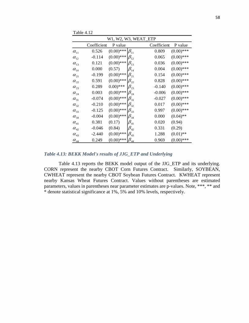
58
Table 4.13: BEKK Model's results of JJG_ETP and Underlying
Table 4.13 reports the BEKK model output of the JJG_ETP and its underlying.
CORN represent the nearby CBOT Corn Futures Contract. Similarly, SOYBEAN,
CWHEAT represent the nearby CBOT Soybean Futures Contract. KWHEAT represent
nearby Kansas Wheat Futures Contract. Values without parentheses are estimated
parameters, values in parentheses near parameter estimates are p-values. Note, ***, ** and
* denote statistical significance at 1%, 5% and 10% levels, respectively.
Table 4.12
Coefficient P value Coefficient P value
0.526 (0.00)*** 0.809 (0.00)***
-0.114 (0.00)*** 0.065 (0.00)***
0.121 (0.00)*** 0.036 (0.00)***
0.000 (0.57) 0.004 (0.00)***
-0.199 (0.00)*** 0.154 (0.00)***
0.591 (0.00)*** 0.828 (0.00)***
0.289 0.00)*** -0.140 (0.00)***
0.003 (0.00)*** -0.006 (0.00)***
-0.074 (0.00)*** -0.027 (0.00)***
-0.210 (0.00)*** 0.017 (0.00)***
-0.125 (0.00)*** 0.997 (0.00)***
-0.004 (0.00)*** 0.000 (0.04)**
0.381 (0.17) 0.020 (0.94)
-0.046 (0.84) 0.331 (0.29)
-2.440 (0.00)*** 1.288 (0.01)**
0.249 (0.00)*** 0.969 (0.00)***
W1, W2, W3, WEAT_ETP
11 11
12 12
13 13
14 14
21 21
22 22
23 23
24 24
31 31
32 32
33 33
34 34
41 41
42 42
43 43
44 44

59
Table 4.14: BEKK Model's results of DAG_ETP and Underlying
Table 4.14 reports the BEKK model output of the DAG_ETP and its underlying.
CORN represent the nearby CBOT Corn Futures Contract. Similarly, SOYBEAN,
WHEAT and SUGAR represent the nearby CBOT Soybean, Wheat and Sugar Futures
Contract. Values without parentheses are estimated parameters, values in parentheses near
parameter estimates are p-values. Note, ***, ** and * denote statistical significance at 1%,
5% and 10% levels, respectively.
Table 4.13
Coefficient P value Coefficient P value
0.240 (0.00)*** 0.966 (0.00)***
0.136 (0.00)*** -0.036 (0.00)***
-0.100 (0.00)*** 0.026 (0.00)***
-0.057 (0.01)** 0.015 (0.00)***
0.002 (0.04)** -0.001 (0.00)***
0.037 (0.00)*** -0.010 (0.00)***
0.563 (0.00)*** 0.870 (0.00)***
0.009 (0.27) -0.003 (0.22)
0.020 (0.01)** -0.005 (0.03)**
0.003 (0.00)*** 0.000 (0.00)***
0.059 (0.01)** -0.004 (0.15)
0.262 (0.00)*** -0.022 (0.11)
0.225 (0.00)*** 0.967 (0.00)***
0.035 (0.00)*** -0.007 (0.23)
0.006 (0.00)*** 0.000 (0.27)
-0.017 (0.06)* 0.003 (0.28)
-0.132 (0.00)*** 0.022 (0.13)
0.069 (0.00)*** -0.010 (0.04)**
0.248 (0.00)*** 0.970 (0.00)***
-0.003 (0.00)*** 0.000 (0.13)
-2.324 (0.00)*** 0.455 (0.00)***
-9.780 (0.00)*** 2.276 (0.00)***
-0.071 (0.88) -0.112 (0.25)
-0.701 (0.14) 0.014 (0.88)
0.034 (0.00)*** 1.000 (0.00)***
CORN SOYBEAN CWHEAT KWHEAT JJG_ETP
44 44
11 11
12 12
13 13
14 14
15 15
21 21
22 22
23 23
24 24
25 25
31 31
32 32
33 33
34 34
35 35
41 41
42 42
43 43
44 44
45 45
51 51
52 52
53 53
54 54
55 55

60
4.5 Magnitude of Volatility Spillovers between ETPs and Underlying
The magnitude of volatility spillover is the summation of the parameters of ARCH
effects and GARCH effect in the BEKK model. The value of magnitude does not matter a
lot, while the difference in magnitude represents the rank of contribution. In Table 4.15,
the findings show that the contribution of volatility spillover from the nearby futures
contracts to ETPs, given they are single commodity based ETPs, is higher than that from
Table 4.14
Coefficient P value Coefficient P value
0.230 (0.00)*** 0.962 (0.00)***
-0.063 (0.00)*** 0.011 (0.10)
-0.275 (0.00)*** 0.248 (0.00)***
0.000 (0.14) 0.000 (0.00)***
0.000 (0.14) 0.000 (0.02)**
0.042 (0.00)*** -0.014 (0.00)***
0.241 (0.00)*** 0.955 (0.00)***
-0.029 (0.45) -0.028 (0.33)
0.000 (0.21) 0.000 (0.00)***
0.000 (0.00)*** 0.000 (0.02)**
-0.027 (0.00)*** 0.016 (0.01)**
-0.004 (0.69) 0.005 (0.47)
0.601 (0.00)*** 0.648 (0.00)***
-0.001 (0.00)*** 0.000 (0.00)***
0.000 (0.54) 0.000 (0.05)*
1.410 (0.00)*** -0.215 (0.00)***
1.801 (0.00)*** -0.235 (0.00)***
6.016 (0.00)*** -1.253 (0.00)***
0.128 (0.00)*** 0.990 (0.00)***
0.027 (0.00)*** -0.002 (0.00)***
1.294 (0.03)** -0.369 (0.01)**
3.426 (0.00)*** -0.777 (0.10)
-17.573 (0.00)*** 9.385 (0.00)***
0.061 (0.01)** -0.029 (0.00)***
0.265 (0.00)*** 0.957 (0.00)***
CORN WHEAT SOYBEAN SUGAR DAG_ETP
55 55
11 11
12 12
13 13
14 14
15 15
21 21
22 22
23 23
24 24
25 25
31 31
32 32
33 33
34 34
35 35
41 41
42 42
43 43
44 44
45 45
51 51
52 52
53 53
54 54
55 55
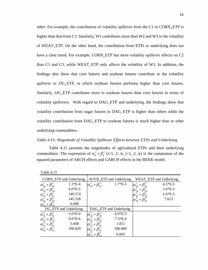
61
other. For example, the contribution of volatility spillover from the C1 to CORN_ETP is
higher than that from C3. Similarly, W1 contributes more than W2 and W3 to the volatility
of WEAT_ETP. On the other hand, the contribution from ETPs to underlying does not
have a clear trend. For example, CORN_ETP has more volatility spillover effects on C2
than C1 and C3, while WEAT_ETP only affects the volatility of W3. In addition, the
findings also show that corn futures and soybean futures contribute to the volatility
spillover to JJG_ETP, in which soybean futures performs higher than corn futures.
Similarly, JJG_ETP contributes more to soybean futures than corn futures in terms of
volatility spillovers. With regard to DAG_ETP and underlying, the findings show that
volatility contribution from sugar futures to DAG_ETP is higher than others while the
volatility contribution from DAG_ETP to soybean futures is much higher than to other
underlying commodities.
Table 4.15: Magnitude of Volatility Spillover Effects between ETPs and Underlying
Table 4.15 presents the magnitudes of agricultural ETPs and their underlying
commodities. The expression of 2 2
ij ij (i=1, 2...k; j=1, 2...k) is the summation of the
squared parameters of ARCH effects and GARCH effects in the BEKK model.
Table 4.15
1.3*E-4 1.7*E-5 4.5*E-5
6.0*E-5 1.6*E-5
140.574 1.6*E-5
145.558 7.613
0.999
5.0*E-6 8.0*E-5
9.0*E-6 7.3*E-4
5.608 1.811
100.829 396.889
0.005
DAG_ETP and UnderlyingJJG_ETP and Underlying
CORN_ETP and Underlying SOYB_ETP and Underlying WEAT_ETP and Underlying2 2
14 14 2 2
14 14 2 2
14 14 2 2
15 15 2 2
34 34 2 2
24 24 2 2
25 25 2 2
41 41 2 2
34 34 2 2
51 51 2 2
42 42 2 2
43 43 2 2
52 52 2 2
43 43
2 2
15 15 2 2
25 25 2 2
25 25 2 2
45 45 2 2
51 51 2 2
51 51 2 2
52 52 2 2
53 53 2 2
54 54

62
CHAPTER 5 CONCLUSIONS
This study aims to investigate the price discovery and volatility spillover effects
between agricultural grain ETPs and their underlying, which are traded in different
markets: the stock markets and the futures markets. Three types of potential results are
assumed: 1) there exists bidirectional price and volatility transmission among ETPs and
underlying components, 2) there exists unidirectional price and volatility transmission
among ETPs and underlying components, 3) there does not exists directional price and
volatility transmission among ETPs and underlying components. An additional purpose is
assumed: the agricultural ETP market has a rising information share in the price discovery
of underlying commodities.
To achieve these goals, this study examines the five most popular agricultural
ETPs: three of them are single commodity based ETPs with multiple futures contract
months, and two of them are multiple commodity based ETPs with nearby contract months.
Due to short history of agriculture ETPs, this study covers all the historical data of each
ETP since inception. Among them, the longest trading history ranges from October 23rd,
2007 to March 14th 2016. All the data of the trading history of each ETPs is obtained from
Yahoo Finance, while all the trading history of the underlying of ETPs, the commodity
futures contracts, is gained from Quandl Database. Then, after data manipulation, all daily
settlement price data is used. Considering the existence of cointegration, this study adopts
Vector Error Correction Model (VEC model) to explore price discovery among ETPs and
underlying components. Following that, we apply Hasbrouck’s (1995) method to measure
the information share of ETPs and underlying components. Lastly, we obtain residuals

63
from each VEC model and apply them into Baba, Engle, Kraft, and Kroner model (BEKK
model) to investigate the volatility spillover effects among ETPs and underlying
components.
From the results of VEC model, this study uncovers that there are unidirectional
and bidirectional price spillover effects existing between certain ETPs and underlying
components in both long-term and short-term. Take the CORN_ETP for example. There
are unilateral relationships from the CORN_ETP to C2 and C3 in the long run, while there
are unilateral relationships from the CORN_ETP to C1 and C2 in the short run. Similarly,
in the long run, there are unilateral relationships from the SOYB_ETP to S2 and S3 and a
bilateral relationship between SOYB_ETP and S1, while there are unilateral relationships
from S2 and S3 to SOYB_ETP in the short run. Furthermore, in the long run, there are
unilateral relationships from the WEAT_ETP to W1 and from W2 to WEAT_ETP, as well
as a bilateral relationship between WEAT_ETP and W3, while there is no evidence of
equilibrium relationships between WEAT_ETP and its underlying commodities in the
short run.
With regard to JJG_ETP and DAG_ETP, there are unilateral relationships from
JJG_ETP to corn futures and Kansas wheat futures in the long run, while there are strong
unilateral relationships from JJG_ETP to corn futures and Kansas wheat futures. In
addition, in the long run, there is a unilateral relationship from corn futures to DAG_ETP,
while there are unilateral relationships from corn futures and wheat futures to DAG_ETP
in the short run.
From the results for information share, this study shows that the information share
of ETPs’ underlying is much higher than ETPs. This means underlying commodities move

64
faster than ETPs when new information comes. Interestingly, in three single commodity
based ETPs, all the nearby futures contracts have the largest information share. This
findings explains that they have more price discovery and move faster than others when
new shocks come in the market. In addition, this study rejects the hypothesis that the
agricultural ETPs have a rising information share in the process of price discovery.
From the results of BEKK model, this study finds that there indeed are
unidirectional and bilateral volatility spillover effects existing between certain ETPs and
their underlying. Take the CORN_ETP for example. The findings show that there are
bidirectional shock transmissions between the CORN_ETP and underlying of C1 and C3
and a unidirectional shock transmission from CORN_ETP to C2. Meanwhile, there are
bidirectional volatility spillovers between the ETP of CORN and underlying of C1, C2 and
C3. Similarly, this also applies to the SOYB_ETP and WEAT_ETP. There are a bi-
directional shock transmissions between the SOYB_ETP and S1, and a unidirectional
shock linkage from SOYB_ETP to S2. And unidirectional volatility spillovers effects exist
from S1 and S3 to SOYB_ETP. In addition, there are bi-directional shock transmissions
between the ETP_WEAT and its underlying of W2, W3, and a unidirectional shock
transmission from W1 to WEAT_ETP. The above findings imply the evidence of bi-
directional volatility spillovers between the WEAT_ETP and W3 and unilateral volatility
spillovers from W1 and W2 to WEAT_ETP.
With regard to JJG_ETP and DAG_ETP, this study uncovers evidences of bi-
directional shock transmissions between the JJG_ETP and corn futures and soybean futures
and unidirectional shock transmissions from Chicago wheat futures and Kansas wheat
futures to JJG_ETP. And there are strong volatility transmissions from JJG_ETP to the
65
corn futures and soybean futures. Thus, it concludes that there are bidirectional volatility
spillovers effect existing between JJG_ETP and corn futures and soybean futures. In
addition, there exist bi-directional shock transmissions between the DAG_ETP and wheat
futures as well as sugar futures, and unidirectional shock transmissions from DAG_ETP to
corn futures as well as soybean futures. Bidirectional volatility spillovers exist between the
DAG_ETP and corn futures as well as sugar futures, and unilateral volatility spillovers
from DAG_ETP to soybean futures and from wheat futures to DAG_ETP.
In the comparison of magnitude to volatility spillover effects, we find that the
contribution of volatility spillovers from the underlying to ETPs and ETPs to the
underlying. When they are single commodity based ETPs, the contributions of nearby
futures contract are always higher than that from distant contracts. However, contributions
from ETPs to underlying do not have a clear trend.
Due to limitations and time constraints, this study does not cover different methods
of price discovery and volatility spillover measurements and other related factors. Further
studies could analyze the volatility spillover effect between agriculture ETPs and their
underlying commodities by focusing on the structural break (different time periods) in
multivariate GARCH models, in addition to developing optimal hedging strategies using
agriculture ETPs that could be adopted by investors.

66
REFERENCES
Aber, Jack W., Dan Li, and Luc Can. "Price volatility and tracking ability of ETFs."
Journal of Asset Management 10.4 (2009): 210-221.
Ascioglu A., M. Aydogdu, R. K. Chou and L. P. Kugele (2006). "An Analysis of Intraday
Patterns in ETF and Common Stock Spreads", working paper.
Ackert L. F. and Y. S. Tian (2000). "Arbitrage and Valuation in the Market for Standard
and Poor's Depositary Receipts", Financial Management, v29, 71-87.
Bodie, Zvi. (1995). On the risk of stocks in the long run. Financial Analysts Journal 51,
18-22.
Ben-David, Itzhak, Francesco Franzoni, and Rabih Moussawi. Do ETFs increase
volatility? No.w20071. National Bureau of Economic Research, 2014.
Borkovec M, Domowitz I, Serbin V, et al. Liquidity and Price Discovery in Exchange-
Traded Funds: One of Several Possible Lessons from the Flash Crash [J]. The
Journal of Index Investing, 2010, 1(2): 24-42.]
Buguk, Cumhur, Darren Hudson, and Terry Hanson. "Price volatility Spillover in
Agricultural Markets: an Examination of US Catfish Markets." Journal of
Agricultural and Resource Economics (2003): 86-99.
Corbet Shaen, and Cian Twomey. "Have Exchange Traded Funds Influenced Commodity
Market Volatility?" International Journal of Economics and Financial Issues 4.2
(2014): 323-335.
DeFusco, A.R, Ivanov I.S. and Karels V. G. (2011). The Exchange Traded Funds' Pricing

67
Deviation: Analysis and Forecasts. Journal of Economics and Finance, 35, 181-
197.
Deville, Laurent. "Exchange Traded Funds: History, Trading and Research." Handbook
of Financial Engineering. Springer US, 2008. 67-98.
Du, Xiaodong, Yu, Cindy L., & Hayes, Dermot J. (2011). Speculation and volatility
spillover in the crude oil and agricultural commodity markets: A Bayesian
Analysis. Energy Economics, 33(3), 497-503.
Engle, Robert, and Debojyoti Sarkar. "Premiums-discounts and exchange traded funds."
Journal Of Derivatives 13.4 (2006): 27.
Figuerola-Ferretti I, Gonzalo J. Modelling and measuring price discovery in commodity
Markets [J]. Journal of Econometrics, 2010, 158(1): 95-107.
Hamilton, James D., and Jing Cynthia Wu. "Effects of Index? Fund Investing On
Commodity Futures Prices." International Economic Review 56.1 (2015): 187-
205.
Hasbrouck J. One security, many markets: Determining the contributions to price
discovery [J]. The journal of Finance, 1995, 50(4): 1175-1199.
Henker, Thomas, and Martin Martens. "Price discovery in HOLDR security baskets and
the Underlying stocks." Available at SSRN 924520 (2006).
Krause, Timothy, and Yiuman Tse. "Volatility and return spillovers in Canadian and US
industry ETFs." International Review of Economics & Finance 25 (2013): 244-
259.
Li, Yanan, & Giles, David E. (2013). Modelling Volatility Spillover Effects Between
Developed Stock Markets and Asian Emerging Stock Markets.

68
Lin, Ching-Chung, and Min-Hsien Chiang. "Volatility effect of ETFs on the constituents
of the Underlying Taiwan 50 Index." Applied Financial Economics 15.18 (2005):
1315-1322.
Madura J. and N. Richie (2005). "Impact of the QQQ on Liquidity, Pricing Efficiency,
and Risk Of the Underlying Stocks", working paper, Susquehanna University.
Noman, Abdullah M., and M. Nakibur Rahman. "Commodity futures indexes and related
Exchange traded notes: Linear and nonlinear adjustment." Journal of Derivatives
& Hedge Funds 19.3 (2013): 189-207.
Park T. H. and Switzer L. N. (1995). "Index Participation Units and the Performance of
Index Futures Markets, Evidence from the Toronto 35 Index Participation Units
Market", Journal of Futures Markets, v15, 187-2000.
Serra, Teresa. (2011). Volatility spillovers between food and energy markets: A
semiparametric Approach. Energy Economics, 33(6), 1155-1164.
Yang J, Leatham D J. Price discovery in wheat futures markets [J]. Journal of
Agricultural and Applied Economics, 1999, 31(02): 359-370.
Yang, Jian, Jin Zhang, and David J. Leatham. "Price and volatility transmission in
international wheat futures markets." Annals of Economics and Finance 4 (2003):
37-50.
Yang, Jian, David Bessler, and David J. Leatham. "Asset storability and price discovery
of Commodity futures markets: A new look." Available at SSRN 322682 (2002).
Yan, Bingcheng, and Eric Zivot. "A structural analysis of price discovery measures."
Journal of Financial Markets 13.1 (2010): 1-19.
Zhao, Jieyuan, and Barry Goodwin. "Volatility spillovers in agricultural commodity

69
markets: An Application involving implied volatilities from options markets."
Selected Paper prepared for presentation at the AAEA & NAREA Joint Annual
Meeting, Pittsburgh, Pennsylvania, and July. 2011.
Top Related