


Languages
Pages
Legal


Preserving Privacy in Data Preparation for
Association Rule Mining
Nan Zhang, Shengquan Wang, and Wei Zhao, Fellow, IEEE
Abstract
We address the privacy preserving association rule mining problem in a distributed system with one data miner
and multiple data providers, each holds one transaction. The literature has tacitly assumed that randomization is the
only effective approach to preserve privacy in such circumstances. We challenge this assumption by introducing
an algebraic techniques based scheme in the data preparation phase. Compared to previous approaches, our new
scheme can identify association rules more accurately but disclose less private information. Furthermore, our new
scheme can be readily integrated as a middleware with existing systems.
Index Terms
Data mining; clustering, classification, and association rules; privacy; singular value decomposition.
I. INTRODUCTION
The goal of data mining is to extract interesting knowledge from large amounts of data [1]. Traditional
data mining algorithms deal with centralized data. Recently, a number of applications on the Internet lead
to a need for mining distributed data. In this circumstance, a privacy concern arises from the distributed
The authors are with the Department of Computer Science, Texas A&M University, College Station, TX 77840. E-mail: {nzhang, swang,
zhao}@cs.tamu.edu.
A preliminary version of this paper is to be presented at the 8th European Conference on Principles and Practice of Knowledge Discovery
in Databases (PKDD), September 2004.

2
data providers. In this paper, we address issues related to production of accurate data mining results, while
preserving the private information in the data being mined.
We will focus on association rule mining, which will be briefly reviewed in the next section. Since
Agrawal, Imielinski, and Swami addressed this problem in [2], association rule mining has been an active
research area due to its wide applications and the challenges it presents. Many algorithms have been
proposed and analyzed [3]–[5]. However, few of them have addressed the issue of privacy protection.
We can classify privacy preserving association rule mining systems into two classes based on their
infrastructures, named Server to Server (S2S) and Client-to-Server (C2S), respectively. In the first category
(S2S), data are distributed across several autonomous entities (servers) [6], [7]. Each server holds a private
database that contains numerous data points (i.e., transactions). The servers collaborate with each other
to identify association rules spanning multiple databases. Since usually only a few servers are involved
in a system (e.g., less than 10), the problem can be modeled as a variation of the secured multi-party
computation [8], which has been extensively studied in cryptography [9].
In the second category (C2S), a system consists of one data miner (server) and large amounts of data
providers (clients) [10], [11]. Each data provider holds only one transaction. Association rule mining is
performed by the data miner on the aggregate transactions provided by the data providers. Online survey
is a typical example of this kind of system, as the system can be modeled as consisting of one data miner
(i.e., the survey analyzer) and thousands of data providers (i.e., the survey respondents). To ensure the
effectiveness of the survey results (e.g., to block multiple votes from a unique IP), the identity of the data
providers cannot be hidden from the data miner. Thus, privacy is of particular concern in this kind of
system. In fact, there has been wide media coverage of the public debate of protecting privacy in online
surveys [12].
Both S2S and C2S systems have wide applications. Nevertheless, we will focus on studying C2S
systems in this paper. Several studies have been carried out on privacy preserving association rule mining
in C2S systems. Most of them have tacitly assumed that an effective approach to preserving privacy is

3
randomization. If we consider the data mining as a two-phase process, which consists of the the data
prepartion phase and the data mining phase, the randomization approach is involved in both phases. We
Fig. 1. 2-phase Data Mining
challenge this assumption by introducing a new scheme that only occurs in the data preparation phase.
Our new scheme integrates algebraic techniques with random noise perturbation. It has the following
important features that distinguish it from previous approaches:
• Our scheme is easy to implement and flexible. Our scheme is involved only in the data preparation
phase and does not require a support recovery procedure in the data mining phase. Thus, our new
scheme is transparent to the data mining process. It can be readily integrated as a middleware with
existing systems.
• Our scheme can identify association rules more accurately but disclose less private information.
Roughly speaking, our scheme selects the most useful features for asssociation rule mining from the
original data and transmits only these features to the data miner. Our simulation data show that for
the same level of accuracy, our system discloses private information about five times less than the
randomization approach.
• We allow explicit negotiation between the data providers and the data miner in terms of the tradeoff
between the accuracy of data mining results and the privacy of data providers. Instead of following
the rules set by the data miner, a data provider can play a role in determining the tradeoff between
accuracy and privacy. This is an important feature because people have a wide variety of attitudes

4
towards privacy. Due to survey results in [13], the net users’ attritudes towards privacy can be
divided into three categories: 7% privacy fundamentalists who are extremely concerned about the use
of their private data, 56% pragmatic majority who are generally willing to provide data if privacy
protection measures can be offered; and 27% marginally concerned who barely care about privacy.
The negotiation feature in our scheme can help the data miner to collaborate with both hard-core
privacy fundamentalists and people comfortable with limited privacy disclosure.
The rest of this paper is organized as follows: In Section II, we brief review previous approaches. We
present our models and introduce our new scheme in Section III. The communication protocol of our
new scheme and its basic components are also provided in this section. In Section IV, we present the
theoretical analysis of the tradeoff between accuracy and privacy in our scheme. The simulation results are
presented in Section V. In Section VI, we present the experimental results on the performance evaluation
of our scheme. Implementation and overhead issues are discussed in Section VII, followed by a final
remark in Section VIII.
II. APPROACHES
In this section, we first overview the definition of association rule mining. Then, we introduce our
models of the data miners. Based on the model, we review the randomization approach, which has been
widely used in the literature of privacy preserving data mining. We will address the problems associated
with the randomization approach, which motivates us to design a new privacy preserving scheme.
A. Association Rule Mining
A motivating example for association rule mining is a survey of hobbies. Each survey respondent
chooses arbitrary number of hobbies from five options: football, soccer, beauty, video games and PC
games. These options are called items. For a survey respondent, the answer to the survey is called a
transaction. As we can see, a transaction is a set of items (e.g., t ={football, soccer}). Given a number
of transactions, association rule mining finds interesting correlation (relationship) between items [1]. For

5
example, suppose that there are 5, 000 survey respondents. The survey analyzer finds that within the 1, 000
respondents who choose video games as their hobbies, there are 800 respondents who also choose PC
games as their hobbies. Based on the survey results, the survey analyzer may infer an association rule
that can be represented as follows.
video games ⇒ PC games [support = 16%, confidence = 80%]. (1)
The support of this rule is the percentage of the respondents who choose both video games and PC
games. Roughly speaking, the confidence is the probability that a respondent who chooses video games
also chooses PC games. Both support and confidence are measures of the validity and trustworthiness of
the association rules. Technically speaking, the main task of association rule mining is to find all frequent
itemsets, which are itemsets that have support larger than a threshold determined by the data miner.
B. Model of Data Miners
Due to the privacy concern introduced to the system, we classify the data miners into two categories.
One category is legal data miners. These data miners always act legally in that they only perform regular
data mining tasks and would never intentionally invade the privacy of the data providers. The other
category is illegal data miners. These data miners would purposely compromise the privacy of the data
providers.
Like adversaries in distributed systems, illegal data miners come in many forms. In most forms, their
behavior is restricted from arbitrarily deviating from the protocol. In this paper, we focus on a particular
sub-class of illegal miners. That is, in our system, illegal data miners are honest but curious: they follow
proper protocols (i.e., they are honest), but they analyze all intermediate communications and received
transactions (i.e., they are curious) to discover private information [9]. Even though it is a relaxation from
the Byzantine behavior, this kind of honest but curious (nevertheless illegal) behavior is common and has
been widely used as the adversary model in the literature.

6
C. Randomization Approach
To prevent invasion of privacy due to the existence of illegal data miners, countermeasures must be
implemented in the data mining system. We briefly review the randomization approach, which is currently
used to preserve privacy in association rule mining.
Based on the randomization approach, the entire data mining process is a two-step process. The first
step is in the data preparation phase. In this step, a data provider first applies the randomization algorithm
to the transaction it holds. Then, the data provider transforms the randomized transaction to the data
miner. In previous studies, several randomization algorithms have been proposed including the cut-and-
paste operator [10] and MASK operator [11]. For example, when the cut-and-paste operator is used, the
data provider first randomly choose an integer j as the number of items that occur in both the original
transaction t and the randomized transaction R(t). After that, the data provider randomly choose j items
from the t and place these items into R(t). Then, for every item a 6∈ t, the data provider tosses a coin
with probability ρ to place a into R(t).
In the second step, the data miner performs association rule mining on the aggregate data. With the
randomization approach, the data miner must first employ a support recovery algorithm which intends to
reconstruct the support of candidate itemsets.
Also in the second step, an illegal data miner may invade privacy by using a privacy data recovery
algorithm on the randomized transactions supplied by the data providers.
Figure 1 depicts the privacy preserving association rule mining system with the randomization approach.
Clearly, any such system should be measured by its capability of both generating accurate association
rules and preventing invasion of privacy.
D. Problems of the Randomization Approach
While the randomization approach is intuitive, researchers have recently identified some problems of
the randomization approach as follows.

7
Fig. 2. randomization approach
• In [10], the authors remarked that if the cut-and-paste operator is applied to a transaction with 10
or more items, it is difficult, if not impossible, for the data provider to contribute to the association
rule mining with its privacy preserved. Furthermore, large itemsets have exceedingly high variances
on the recovered support. Similar problems exist with other randomization operators as they share
the similar scheme on the randomization of the original data.
An approach was proposed in [10] to solve this problem. In the approach, all data providers that
hold transactions with 10 or more items do not transfer the randomized transaction to the data miner.
Unfortunately, this approach prevents many frequent itemsets that contain 4 or more items from being
discovered by the data miner.
• In [14], the authors showed that the spectral properties of randomized data could help curious
data miners to separate noise from private data. Based on random matrix theory, they proposed
a filtering method to reconstruct private data from the randomized data set. They demonstrated that
the randomization approach preserves very little privacy in many cases. Although their work is based

8
on the randomization approach for privacy preserving data classification, we believe that the similarity
between randomization operators in association rule mining and data classification makes the problem
inherent in the randomization approach.
• The randomization approach also suffers in efficiency. Since the privacy preserving mechanism is
not restricted to the data preparation phase, it puts a heavy load on (legal) data miners at run time
(because of the support recovery) [15]. It is shown that the cost of mining randomized data set is
well within an order of magnitude in respect to that of mining original data set.
We explore the reasons behind these problems as given below.
• We note that previous randomization approaches are transaction-invariant. That is, the same pertur-
bation algorithm is applied to all data. Since more items in the original transaction always result in
more “real” items to be included in the randomized transaction, privacy protection on transactions
with a large size (e.g., |t| > 10) are doomed to failure.
• Previous randomization approaches are item-invariant. All items in the original transaction have the
same probability of being included in the perturbed transaction. No specific operation is performed
to preserve the correlation between different items. Thus, a lot of “real” items in the perturbed
transactions may not appear in any frequent itemset. That is, the disclosure of these items does not
contribute to the mining of association rules.
We remark that the transaction-invariant and item-invariant properties are inherent in the randomization
approach. The reason is that in a system using randomization approach, the communication is one-way:
from the data providers to the data miner. As such, a data provider cannot obtain any specific guidance
on the perturbation of its transaction from the (legal) data miner, nor can the data providers learn the
correlation between the items. Thus, a data provider has no choice but to use a transaction-invariant and
item-invariant approach.
This observation motivates us to develop a new scheme that allows two-way communication between
the data miner and the data providers. The two-way communication helps preserving privacy while not

9
incurring too much overhead. Thereby, we significantly improve the performance in terms of accuracy,
privacy, and efficiency. We describe the new scheme in the next section.
III. COMMUNICATION PROTOCOL AND RELATED COMPONENTS
In this section, we introduce our new scheme including the communication protocol and its basic
components.
A. Description of Our New Scheme
Fig. 3. our new scheme
Figure 2 depicts the infrastructure of a system using our new scheme. Our scheme has two key
components, perturbation guidance (PG) in the data miner server side and perturbation in the data provider
client side. Compared to the randomization approach, our scheme does not have the support recovery
component. Instead, the association rule mining is performed on the perturbed transactions (R(t)) directly.
Thus, our scheme is restricted to the data preparation stage and does not put a heavy load on the data
miner by recovering the support at run time.

10
Our scheme is a three-step process. In the first step, the data miner negotiates different perturbation level
k with different data providers. The larger k is, the more contribution R(t) will make to the association rule
mining task. The smaller k is, the more private information is preserved. Thus, a privacy fundamentalist
can choose a small k to preserve its privacy while a privacy unconcerned data provider can choose a large
k to contribute to the association rule mining.
The second step is to transmit the perturbed transactions from the data providers to the data miner.
Since each data provider comes at a different time (e.g., different survey respondents take the survey at
different time), this step can be considered as an iterative process. In each stage, the data miner dispatches
a reference (perturbation guidance) Vk to a data provider Pi. Here Vk depends on the perturbation level
kthat is negotiated by the data miner and the data provider Pi in the first step. Based on the received Vk,
the perturbation component of Pi computes the perturbed transaction R(t) from its original transaction
t. Then, Pi transmits R(t) to the perturbation guidance (PG) component of the data miner. The PG
component then updates Vk based on R(t) and forwards R(t) to the association rule mining process. A
curious data miner can also obtain R(t). In this case, the curious data miner uses private data recovery
algorithm to compromise privacy in R(t).
In the third step, the perturbed transactions received by the data miner are used by the association rule
mining process. Association rules are identified and delivered to the data miner.
The key here is to properly design Vk so that correct guidance can be given to the data providers on how
to perturb the transactions. In our scheme, we let Vk be an algebraic quantity derived from the currently
received, yet perturbed transactions. The details of computing Vk will be presented as a basic component
of our scheme.
B. Notions of Transactions
Before presenting the details of the communication protocol and its basic components, we first introduce
some notions of the data set. Let I be a set of n items (i.e., I = {a1, . . . , an}. Suppose that there are
m data providers in the system. Each data provider Ci holds a transaction ti, which is a subset of I . We

11
represent the data set by an m×n matrix T = [a1, . . . , an] = [t1; . . . ; tm] 1. An example of the transaction
matrix T is shown in Table I. Let 〈T 〉ij be the element of T with indices i and j. The element 〈T 〉ij
represents whether item j is in transaction ti. Suppose that transaction t1 contains items a1 and a2. The
first row of the matrix has 〈T 〉1,1 = 〈T 〉1,2 = 1.
TABLE I
AN EXAMPLE OF A TRANSACTION MATRIX
a1 a2 · · · an
t1 1 1 · · · 0
......
.... . .
...
tm 1 0 · · · 1
An itemset B ⊆ I is an h-itemset if and only if B contains h items (i.e., |B| = h). The support of B
is the percentage of the transactions in the data set that contain B. That is,
supp(B) =|{t ∈ T |B ⊆ t}|
m. (2)
An h-itemset B is frequent if supp(B) ≥ min supp, where min supp is a predefined minimum threshold
of support. Refer to the “survey of hobbies” example in the above subsection, {video games, PC games}
is a frequent 2-itemset with support 0.16. The set of frequent h-itemsets is denoted by Lh.
C. The Communication Protocol
We now describe the communication protocol of our new scheme. The negotiation between the data
miner and data providers is shown in Protocol 1. On the side of data miner server, there are two threads that
perform the operations in Protocol 2 and Protocol 3 iteratively after the negotiation. For a data provider,
it performs the operations in Protocol 4 to perturb and transmit its transaction to the data miner.
1Here ti and ai are used somewhat ambiguously. In the context of association rule mining, ti is a transaction and ai is an item. In the
context of matrix, ti represents a row vector in T and ai represents a column vector in T .
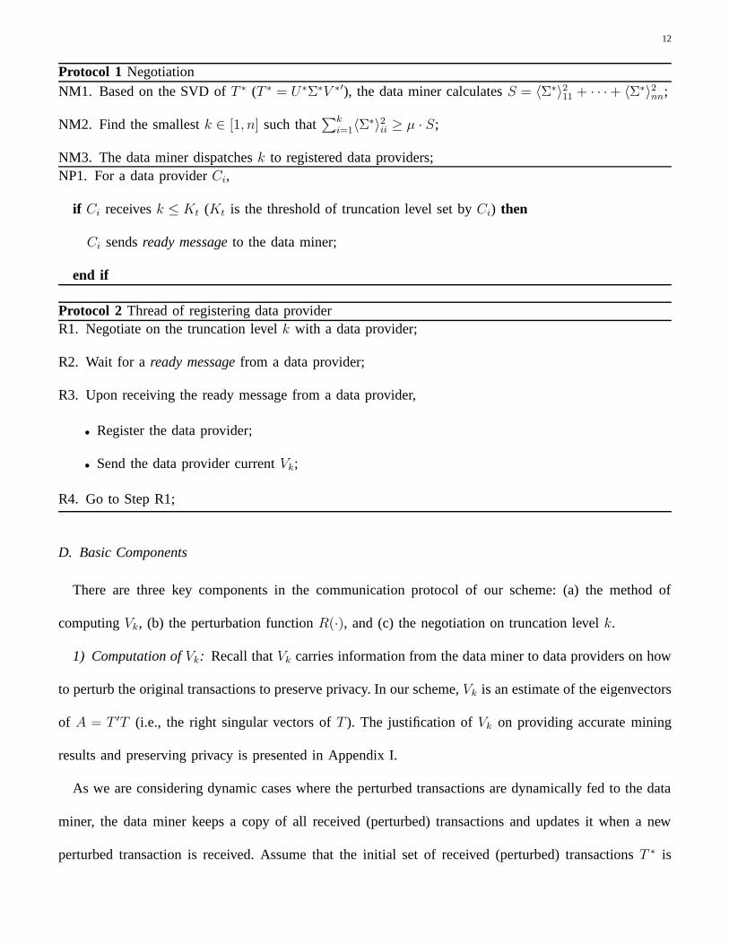
12
Protocol 1 NegotiationNM1. Based on the SVD of T ∗ (T ∗ = U∗Σ∗V ∗′), the data miner calculates S = 〈Σ∗〉211 + · · ·+ 〈Σ∗〉2nn;
NM2. Find the smallest k ∈ [1, n] such that∑k
i=1〈Σ∗〉2ii ≥ µ · S;
NM3. The data miner dispatches k to registered data providers;NP1. For a data provider Ci,
if Ci receives k ≤ Kt (Kt is the threshold of truncation level set by Ci) then
Ci sends ready message to the data miner;
end if
Protocol 2 Thread of registering data providerR1. Negotiate on the truncation level k with a data provider;
R2. Wait for a ready message from a data provider;
R3. Upon receiving the ready message from a data provider,
• Register the data provider;
• Send the data provider current Vk;
R4. Go to Step R1;
D. Basic Components
There are three key components in the communication protocol of our scheme: (a) the method of
computing Vk, (b) the perturbation function R(·), and (c) the negotiation on truncation level k.
1) Computation of Vk: Recall that Vk carries information from the data miner to data providers on how
to perturb the original transactions to preserve privacy. In our scheme, Vk is an estimate of the eigenvectors
of A = T ′T (i.e., the right singular vectors of T ). The justification of Vk on providing accurate mining
results and preserving privacy is presented in Appendix I.
As we are considering dynamic cases where the perturbed transactions are dynamically fed to the data
miner, the data miner keeps a copy of all received (perturbed) transactions and updates it when a new
perturbed transaction is received. Assume that the initial set of received (perturbed) transactions T ∗ is

13
Protocol 3 Thread of receiving transactionT1. Wait for a perturbed transaction R(t) from a data provider;
T2. Upon receiving the transaction from a registered data provider,
• Update Vk based on the recently received perturbed transaction;
• Deregister the data provider;
T3. Go to Step T1;
Protocol 4 Transaction perturbationP1. Negotiate on the truncation level k with the data miner;
P2. Send the data miner a ready message indicating that this provider is ready to contribute to the mining
process;
P3. Wait for a message that contains Vk from the data miner;
P4. Upon receiving the message from the data miner,
• Compute R(t) based on t and Vk;
P5. Transfer R(t) to the data miner;
empty 2. Every time when a perturbed transaction R(t) is received, T ∗ is updated by appending R(t)
to the bottom of T ∗. Thus, T ∗ is the matrix of currently received (perturbed) transactions. We derive Vk
from T ∗.
In particular, the computation of Vk is done in the following steps. Using singular value decomposition
(SVD) [16], we decompose T ∗ as (3), where Σ∗ = diag(s1, . . . , sn) is a diagonal matrix with s1 ≥ · · · ≥ sn.
T ∗ = U∗Σ∗V ∗′. (3)
The numbers s2i make up the eigenvalues of A∗ = T ∗′T ∗. V ∗ is an n× n unitary matrix composed of the
eigenvectors of A∗.
Vk is composed of the k eigenvectors of A∗ that are associated with the largest k eigenvalues of A∗. If
2T ∗ may also contain some transactions provided by privacy-careless data providers

14
V ∗ = [v1, . . . , vn], we have
Vk = [v1, . . . , vk]. (4)
Thus, we call Vk as the k-truncation of V ∗. Several incremental algorithms have been proposed to update
Vk when a perturbed transaction is received by the data miner [17], [18]. The computing cost of updating
Vk is addressed in Sect. VII.
As we will see in Sect. IV, k plays a critical role in balancing accuracy and privacy. We will also show
that by using Vk in conjunction with R(·), which is to be discussed next, we can achieve both desired
accuracy and privacy protection.
2) Perturbation function: Recall that once a data provider receives Vk from the data miner, the data
provider applies a perturbation function R(·) to its transaction t. The result is a perturbed transaction
R(t) that will be transmitted to the data miner. The computation of R(t) is defined as follows. First, for
a given Vk, the transaction t is transformed by t = tVkV′k . Note that the elements of the vector t may
not be integers. Algorithm 5 is employed to round t to 0 or 1. In this algorithm, ρt is a pre-defined
parameter. Finally, for the completeness of our work, we introduce an optional procedure to enhance the
privacy preserving capability of the system, which is shown in Algorithm 6. A data provider may use
the protocol to insert additional noise into R(t). In the protocol, ρm is a parameter determined by the
data provider. The higher ρm is, the more noise is inserted into the perturbed transaction. We remark that
this protocol is optional and is only needed by privacy fundamentalists. An example of the perturbation
process is provided in Appendix II.
3) Negociation on truncation level: In order to retain enough information for association rule mining
after the transformation from t to R(t), a textbook heuristic is to make the sum of the k eigenvalues
associated with the retained eigenvectors of A∗ larger than 85% of the sum of the eigenvalues of A∗ (i.e.,
µ = 85%) [16], [19]. The perturbation level k is usually large at the beginning but decreases and stabilizes
to be fairly small (e.g., less than 1% of n) soon. Thus, in the theoretical analysis of our scheme, we consider
the perturbation level k as a predetermined parameter rather than a variable updated throughout the data

15
Algorithm 5 Mapping
Let 〈t〉i be the element of vector t with index i. Similar notations apply to other vectors.
for every element 〈t〉i in t do
if 〈t〉i ≥ 1 − ρt then
〈R(t)〉i = 1
else
〈R(t)〉i = 0
end if
end for
Algorithm 6 Random-noise perturbationfor every item ai /∈ t do
Choose a real number j uniformly at random on [0, 1]
if j ≥ 1 − ρm then
〈R(t)〉i = 1
end if
end for
preparation process.
We have described the communication protocol of our scheme and its key components. We now discuss
the accuracy and privacy measures of our scheme.
IV. ANALYSIS ON ACCURACY AND PRIVACY
In this section, we analyze our new scheme. We define measures for accuracy and privacy and derive
their bounds, in order to provide guidelines for the tradeoff between these two measures and hence help
system managers setting parameter. We also show the simulation and experimental results of our scheme
on real datasets. For the simplicity of our discussion, we do not consider the optional random noise
insertion procedure in Algorithm 6.

16
A. Accuracy Measure
An accuracy measure should reflect the capability of the system that can correctly identify association
rules in a given dataset. We define the accuracy measure as the error of the support of frequent itemsets.
This is because that the main task of association rule mining is to identify frequent itemsets with support
larger than a threshold min supp. There are two kinds of errors: a) false drops, which are unidentified
frequent itemsets, and b) false positives, which are itemsets incorrectly identified to be frequent.
We now formally define our accuracy measure. Given itemset Ij , let supp(Ij) and supp′(Ij) be the
support of Ij in the original transactions T and the perturbed transactions R(T ), respectively. Recall that
the set of frequent h-itemsets in T is Lh. We define the errors on false drops and false positives as follows.
Definition 4.1: Given itemset size h, the error on false drops, ρh1 , and the error on false positives, ρh
2 ,
are defined as
ρh1 = max
Ij∈Lh
(supp(Ij) − supp′(Ij)), (5)
ρh2 = max
Ij 6∈Lh
(supp′(Ij) − supp(Ij)). (6)
We define our accuracy measure, degree of accuracy, as the maximum value of ρh1 and ρh
2 on all sizes of
itemsets.
Definition 4.2: The degree of accuracy in a privacy preserving association rule mining system is defined
as γ = maxh≥1 max(ρh1 , ρ
h2).
Based on the definition, we derive an upper bound on the accuracy measure.
Theorem 4.3: In our system, the degree of accuracy γ satisfies
γ ≤ σ2k+1
m
(
1 + max
{
1 − (1 − ρt)2
(1 − ρt)2,1 − ρt
ρt
})
, (7)
where σ2k+1
is the (k+1)th largest eigenvalue of A = T ′T . In particular, when ρt = (3−√
5)/2, γ reaches
its lowest upper bound at γ ≤ 2.618σ2k+1
/m.
The proof of Theorem 4.3 can be found in Appendix III. Our bound on accuracy measure is fairly small
when the number of transactions (m) is sufficiently large. This is usually the case in reality. Actually, our

17
scheme tends to enlarge the support of frequent itemsets and reduce the support of infrequent itemsets.
Thus, the upper bound is not always tight. We can observe this trend from the experimental results, which
will be presented in Section VI.
B. Privacy Measure
In our system, the data miner cannot infer the original transaction t from a perturbed transaction R(t)
deterministically because VkV′k is a singular matrix with its determinant det(VkV
′k) = 0 (i.e., it does not
have an inverse matrix). To measure the probability that an item in t can be identified from R(t), we need
a privacy measure.
Due to survey results in [12], a data provider (e.g., net user) always has a strong will of filtering out
“unwanted” data (i.e., data not contribute to the mining of association rules) before transmitting its private
data to the data miner. Given transaction t, an item ai in t is unwanted if ai does not appear in any frequent
itemset (i.e., ∀h ≥ 1, ai 6∈ {Lh|Lh ⊆ t}). That is, the disclosure of ai (i.e., ai ∈ R(t)) does not contribute
to the mining of association rules. We measure privacy by the probability that an “unwanted” item is
included in the perturbed transaction. Formally speaking, our privacy measure, named level of privacy, is
defined as follows.
Definition 4.4: Given transaction t, an item ai ∈ t is unwanted if and only if there does not exist any
frequent itemset I ⊆ t such that ai ∈ I . We define the level of privacy as the probability that an infrequent
item in t is included in the perturbed transaction R(t). That is, the level of privacy is defined as
δ = Pr{ai ∈ R(t)|ai is unwanted in t}. (8)
As we can see from the definition, a higher level of privacy results in a higher probability of privacy
invasion. With an approximation, we derive an upper bound on the level of privacy in our scheme.
Theorem 4.5: With properly set parameters, the level of privacy in our system is bounded by
δ<∼1 −√
σ2k+1
+ · · ·+ σ2n
σ21 + · · ·+ σ2
n
, (9)
where σ2i is the ith largest eigenvalue of A = T ′T .

18
The proof of Theorem 4.5 can be found in Appendix IV. Because of the uncertainty on the rounding off
operation in Algorithm 5, this bound is not tight.
As we can see from Theorem 4.3 and Theorem 4.5, there is a tradeoff between accuracy and privacy in
our system. The upper bound of the degree of accuracy is in proportion to σ2k+1
. The level of privacy is a
decreasing function of σ2k+1
. The larger the perturbation level k is, the more unwanted items are disclosed
to the data miner, and the more frequent itemsets can be correctly identified.
V. SIMULATION RESULTS
In this section, we present the simulation results of our scheme on a randomly generated dataset. The
experimental results on a real dataset will be presented in the next section.
The randomly generated dataset consists of 2, 000 transactions. Let there are 20 items in the dataset.
Each transaction is a subset of the 20 items. We represent the dataset by a 2, 000 × 20 matrix T . The
first 19 columns (items) of T , a1, . . . , a19, are independently generated. The 20th column is set to be the
same as the 10th column (i.e., a10 = a20). The first item a1 has a probability of 0.6 to be included in a
transaction. All other columns have probability of 0.1 to be included in a transaction. Thus, the expected
support of a1 is 0.6. The expected support of every other item is 0.1. Since a10 = a20, the expected
support of {a10, a20} is 0.1. We set min supp = 0.09 as the threshold (lower bound) on the support of a
frequent itemset.
In the randomly generated dataset, the support of {a1} and {a10, a20} are listed as follows.
support of {a1} = 0.6085, support of {a10, a20} = 0.0985. (10)
As we can see, these two itemsets have support much higher than other 1-itemsets and 2-itemsets,
respectively. The left part of Figure 3 shows the original dataset. In the original dataset, the total number
of appearance of all items is 4929 times including 1217 times of a1, 197 times of a10, 197 times of a20,
and 3318 times of the other items.

19
In our simulation, we set the parameters as µ = 0.85 (in Protocol 1), ρt = 0.8 (in Algorithm 5),
and µm = 0 (in Algorithm 6). The data miner updates Vk when every 10 transactions are received. The
truncation level k calculated from Protocol 1 is listed as follows. The right part of Fig. 3 shows the
TABLE II
TRUNCATION LEVEL k
k 7 6 5 4 3 2
Transaction No. 1 − 20 21 − 50 51 − 90 91 − 120 121 − 200 201 − 2000
dataset after perturbation. In the perturbed dataset, the total number of appearance of all items is 1646
times including 1217 times of a1, 197 times of a10, 197 times of a20, and 35 times of the other items.
The association rule mining results are stated as follows.
{a1}, with support 0.6085 and {a10, a20}, with support 0.0985. (11)
As we can see, the support of “interesting” itemsets are perfectly recovered with the degree of accuracy
γ = 0. The privacy is well preserved with the level of privacy δ = 1.05%.
Fig. 4. comparison of between original and perturbed transactions

20
VI. EXPERIMENTAL RESULTS ON A REAL DATASET
In this section, we make a comparison between our approach and the cut-and-paste randomization
approach [10] by experimental results on a real dataset. We use a real world dataset named “BMS
Webview 1” [20], which contains web click stream data of several months from the e-commerce website
of a leg-care company. The dataset contains 59, 602 transactions and 497 items.
We randomly choose 10, 871 transactions from the dataset as our test band. The maximum transaction
size is 181. The average transaction size is 2.90. There are 325 transactions (2.74%) that contains 10 or
more items. We set the support threshold min supp to be 0.2%. There are 798 frequent itemsets including
259 1-itemset, 350 2-itemsets, 150 3-itemsets, 37 4-itemsets and two 5-itemsets.
As a compromise between privacy and accuracy, the cutoff parameter Km of cut-and-paste random-
ization operator is set to 7. The truncation level k of our approach is set to 6. Since both our approach
and the cut-and-paste operator use the same method to add random noise, we compare the results before
noise is added. Thus we set ρm = 0 for both our approach and the cut-and-paste randomization operator.
0.1 0.2 0.3 0.4 0.5 0.6 0.7 0.8 0.9 10.2
0.4
0.6
0.8
1
1.2
1.4
1.6
1.8
ρt
degr
ee o
f acc
urac
y (%
)
Our perturbation algorithm Previous approach: cut−and−paste
Fig. 5. accuracy
The solid line in Figure 4 shows the change of degree of accuracy (max{ρ1, ρ2}) of our approach with
the parameter ρt. The dotted line shows the degree of accuracy when the cut-and-paste randomization
operator is used. As we can see, our approach always identifies association rules more accurately than

21
the cut-and-paste approach.
0 0.1 0.2 0.3 0.4 0.5 0.6 0.7 0.8 0.9 10
0.1
0.2
0.3
0.4
0.5
0.6
0.7
0.8
Deg
ree
of P
rivac
y
ρt
Our perturbation algorithmPrevious approach: cut−and−paste
Fig. 6. privacy
The level of privacy in the same setting is presented in Fig. 5. As we can see, our approach preserves
privacy better than the cut-and-paste operator when ρt > 0.1. Thus, our approach is better on both privacy
and accuracy issues when 0.1 ≤ ρt ≤ 1. From the figures, we observe a recommendation for the data
providers as that ρt ∈ [0.7, 0.8] is suitable for hard-core privacy fundamentalists and ρt ∈ [0.2, 0.3] is
recommended to privacy marginally concerned people.
In particular, we analyze all 2-itemsets in the real dataset to show that our scheme tends to enlarge the
support of frequent itemsets and reduce the support of infrequent itemsets. The result is shown in Fig. 6.
The x-axis is the support of 2-itemsets in the original dataset. The y-axis is the support of itemsets in
the perturbed dataset. The figure intends to show how effectively our system blocks the unwanted items
from being divulged. If a system preserves privacy perfectly, we should have y equal to zero when x
is less than min supp. The data in Fig. 6 shows that almost all 2-itemsets with support less than 0.2%
(233, 368 unwanted 2-itemsets) have been blocked. That is, the privacy has been successfully protected.
Meanwhile, the supports of frequent 2-itemsets are enlarged. This should help the data miner to identify
frequent itemsets from additional noises.
22
0 50 100 150 200
50
100
150
200
250
Support in Original Transactions
Sup
port
in P
ertu
rbed
Tra
nsac
tions
k = 6 out of 497, ρt = 0.4
Support in R(T) (× 10−4)Support in T (× 10−4)
233,368 2−itemsets
13641 2−itemsets
Fig. 7. comparison of 2-itemsets supports between original and perturbed transactions
VII. IMPLEMENTATION
A prototypical system for privacy preserving mining of association rules has been implemented using
our new scheme. The system is designed on web browsers and servers for the application of online
surveys. Visitors taking surveys through web browsers are considered to be data providers. The web server
conducting surveys is considered to be the data miner. We implement the data perturbation algorithm as
custom code on the web browsers. The PG (perturbation guidance) part of the data miner is implemented
as custom code on the web server. All custom codes are component-based plug-ins that one can easily
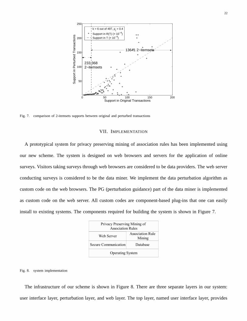
install to existing systems. The components required for building the system is shown in Figure 7.
Fig. 8. system implementation
The infrastructure of our scheme is shown in Figure 8. There are three separate layers in our system:
user interface layer, perturbation layer, and web layer. The top layer, named user interface layer, provides

23
interface to data providers and the data miner. The middle layer, named perturbation layer, realizes our
privacy preserving scheme and exploits the bottom layer to transfer information. The bottom layer, named
web layer, consists of web servers and web browsers. As an important feature of our system, the details
of data perturbation on the middle layer are transparent to both data providers and the data miner. The
Fig. 9. system infrastructure
overhead of our implementation is substantially smaller than the randomization approach in the context of
online survey. The time-consuming part of the cut-and-paste randomization approach, which is the support
recovery procedure, occurs in the association rule mining process. The support recovery algorithm needs
to compute the partial support of all candidate itemsets for each transaction size, which will result in a
significant overhead.
In our system, the only overhead (possibly) incurred on the data miner is to update the perturbation
guidance Vk. Many SVD updating algorithms have been proposed including SVD-updating, folding-in
and recomputing the SVD [17], [18]. Since T ∗ is usually a sparse matrix, the complexity of updating
SVD can be considerably reduced to O(n). Besides, this overhead is not on the critical time path of the
mining process. It occurs during data collection instead of data mining process. Note that the transmitted
“perturbation guidance” Vk is of length k · n. Since k is always a small number (e.g., k ≤ 10), the
communication overhead incurred by our introduction of two-way communication is not significant.
VIII. FINAL REMARKS
In this paper, we propose a new scheme on privacy preserving mining of association rules. Compared
with previous approaches, we introduce a two-way communication mechanism between the data miner

24
and data providers with little overhead. In particular, we let the data miner send a perturbation guidance to
the data providers. Using this intelligence, the data providers distort the data transactions to be transmitted
to the miner. As a result, our scheme identifies association rules more precisely than previous approaches
and at the same time protects privacy more effectively.
Our work is preliminary and many extensions can be made. In addition to using a similar approach in
data classification [21], we are currently investigating how to apply the approach to clustering problems.
We would like to investigate a new behavior model that is stronger than the honest-but-curious model,
and can be dealt with by our scheme.
REFERENCES
[1] J. Han and M. Kamber, Data Mining Concepts and Techniques. Morgan Kaufmann, 2001.
[2] R. Agrawal, T. Imielinski, and A. Swami, “Mining association rules between sets of items in large databases,” in Proc. ACM SIGMOD
Int. Conf. on Management of Data, 1993, pp. 207–216.
[3] R. Agrawal and R. Srikant, “Fast algorithms for mining association rules in large databases,” in Proc. Int. Conf. on Very Large Data
Bases, 1994, pp. 487–499.
[4] J. S. Park, M. S. Chen, and P. S. Yu, “An effective hash-based algorithm for mining association rules,” in Proc. ACM SIGMOD Int.
Conf. on Management of Data, 1995, pp. 175–186.
[5] M. Fang, N. Shivakumar, H. Garcia-Molina, R. Motwani, and J. D. Ullman, “Computing Iceberg queries efficiently,” in Proc. Int. Conf.
on Very Large Data Bases, 1998, pp. 299–310.
[6] J. Vaidya and C. Clifton, “Privacy preserving association rule mining in vertically partitioned data,” in Proc. ACM SIGKDD Int. Conf.
on Knowledge discovery and data mining, 2002, pp. 639–644.
[7] M. Kantarcioglu and C. Clifton, “Privacy-preserving distributed mining of association rules on horizontally partitioned data,” in Proc.
ACM SIGMOD Workshop on Research Issues on Data Mining and Knowledge Discovery, 2002, pp. 24–31.
[8] Y. Lindell and B. Pinkas, “Privacy preserving data mining,” Advances in Cryptology, vol. 1880, pp. 36–54, 2000.
[9] O. Goldreich, Secure Multi-Party Computation. Cambridge Univeristy Press, 2004.
[10] A. Evfimievski, R. Srikant, R. Agrawal, and J. Gehrke, “Privacy preserving mining of association rules,” in Proc. ACM SIGKDD Intl.
Conf. on Knowledge Discovery and Data Mining, 2002, pp. 217–228.
[11] S. J. Rizvi and J. R. Haritsa, “Maintaining data privacy in association rule mining,” in Proc. Int. Conf. on Very Large Data Bases,
2002, pp. 682–693.
[12] J. Hagel and M. Singer, Net Worth. Harvard Business School Press, 1999.

25
[13] L. F. Cranor, J. Reagle, and M. S. Ackerman, “Beyond concern: Understanding net users’ attitudes about online privacy,” AT&T
Labs-Research, Tech. Rep. TR 99.4.3, 1999.
[14] H. Kargupta, S. Datta, Q. Wang, and K. Sivakumar, “On the privacy preserving properties of random data perturbation techniques,” in
Proceedings of the 3rd IEEE International Conference on Data Mining. IEEE Press, 2003, pp. 99–106.
[15] S. Agrawal, V. Krishnan, and J. R. Haritsa, “On addressing efficiency concerns in privacy-preserving mining,” in Proceedings of the
9th International Conference on Database Systems for Advanced Applications. Springer Verlag, 2004, pp. 439–450.
[16] G. H. Golub and C. F. V. Loan, Matrix Computations. Johns Hopkins University Press, 1996.
[17] J. R. Bunch and C. P. Nielsen, “Updating the singular value decomposition,” Numerische Mathematik, vol. 31, pp. 111–129, 1978.
[18] M. Gu and S. C. Eisenstat, “A stable and fast algorithm for updating the singular value decomposition,” Yale University, Tech. Rep.
YALEU/DCS/RR-966, 1993.
[19] I. T. Jolliffe, Principle Component Analysis. Springer Verlag, 1986.
[20] Z. Zheng, R. Kohavi, and L. Mason, “Real world performance of association rule algorithms,” in Proc. ACM SIGKDD Int. Conf. on
Knowledge Discovery and Data Mining, 2001, pp. 401–406.
[21] N. Zhang, S. Wang, and W. Zhao, “On a new scheme on privacy preserving data classification,” Texas A&M University, Tech. Rep.
TAMU/CS 2004-10-5, 2004.
[22] B. Nobel and J. W. Daniel, Applied linear algebra. Prentice-Hall, 1988.

26
APPENDIX I
APPENDIX: JUSTIFICATION OF Vk
The main part of a privacy preserving association rule mining system is the data perturbation mechanism
employed by the data providers. In current techniques, randomization operator is used to perturb original
transactions. As we described in Section II, an item-invariant randomization operator leaves the correlation
between different items unconsidered. We investigate the item correlation to improve accuracy of mining
results.
Specifically, our data perturbation algorithm preserves the support of 2-itemsets. The intuition behind
our approach can be stated as follows. The PG part of the data miner maintains an estimation of the
support of all 1-itemsets and 2-itemsets. Based on the estimation, PG tells the data providers which
itemsets are more likely to be frequent itemsets. We know that no superset of an infrequent itemset is
frequent (anti-monotone). A data provider may safely remove all infrequent 1-itemsets and 2-itemsets
because they cannot appear in any frequent itemset 3 or more items either.
Readers may raise a question that why we choose to maintain the support of 1-itemsets and 2-itemsets
instead of 1, 2, and 3-itemsets or 1-itemsets only? For the first question, the main reason is that the
large number of 3-itemsets (n3) could impose serious overhead on the system. Besides, as we can see in
Appendix III, our algorithm also preserves the support of itemsets with 3 or more items.
On the other hand, if we choose to maintain the support of 1-itemsets only, we cannot remove many
items from original transactions to protect privacy. Roughly speaking, if {ai, aj}, {aj, ak}, and {ai, ak}
are all frequent, we have a fairly high probability that {ai, aj, ak} is also frequent. However, if both ai and
aj are frequent, the probability that {ai, aj} is frequent is much smaller. Thus, in order to guarantee that
all frequent 2-itemsets can be preserved, we cannot remove many items from the original transactions.
Now we will show that our data perturbation algorithm successfully preserves the support of 2-itemsets.
Here we consider the case when Vk is the k-truncation of the accurate eigenvectors of T ′T . In reality, the
value of Vk has to be estimated from the current copy of T ∗. Fortunately, the value of Vk converges well

27
to its accurate value. Besides, the convergence is fairly fast in most cases. The proof of convergence is
presented in Appendix V.
Consider A = T ′T
A = T ′T =
a1 · a1 · · · a1 · an
... ai · aj
...
an · a1 · · · an · an
(I.12)
where ai · aj is the dot product of ai and aj .
ai · aj =
m∑
h=1
〈ai〉h〈aj〉h (I.13)
Note that
ai · aj
m= support of {ai, aj}. (I.14)
Thus, we may preserve the support of 2-itemsets by a precise approximation of A. In particular, we use
truncated eigenvectors of A to perturb the original transactions T into T .
Given transaction matrix T , define the perturbed transaction T = TVkV′k .
T = [t1, t2, . . . tm]′ (I.15)
Vk = [v1, v2, . . . , vk] (I.16)
T = TVkV′k = [t1VkV
′k, t2VkV
′k, . . . , tmVkV
′k]. (I.17)
With some algebriac manupulation we have
A = T ′T = VkV′kT
′TVkV′k (I.18)
= VkV′kV (Σ′Σ)V ′VkV
′k (I.19)
= VkΣ′ΣV ′
k (I.20)
= σ2
1v1v′1 + · · ·+ σ2
kvkv′k (I.21)
Thus, A is the optimal rank-k approximation of A [16]. In other words, we preserve the support of
2-itemsets while cutting off its eigenvectors.

28
Our data perturbation algorithm also preserves the privacy of data providers. The data miner cannot
deduce the original t from t because VkV′k is a singular matrix with det(VkV
′k) = 0, which means that
VkV′k does not have an inverse matrix.
APPENDIX II
APPENDIX: EXAMPLE OF TRANSACTION PERTUBATION
As we have shown in Appendix I, we can reach a precise approximation of A = T ′T by perturbing t
to t = tVkV′k. Besides this “truncated eigenvectors” perturbation, we need a function to map the values
of t ∈ [0, 1] to integer values R(t) ∈ {0, 1}. Although the truncation of eigenvectors has already inserted
some “noise” items into the transactions, we still need to add more “noise” items. These tasks are done
by the Alg. 5 and Alg. 6. Here we use an example to illustrate the algorithms involved in the perturbation
process.
Example 2.1: A data provider Ci holds a transaction t = [1, 1, 0, 1, 1, 1, 0, 0]. After negotiating with the
data miner, Ci receives Vk (k = 2) from the data miner as follows.
V ′k =
0.30 0.43 0.38 0.28 0.32 0.43 0.35 0.27
−0.50 0.08 −0.01 0.37 −0.03 0.05 −0.45 0.61
(II.22)
Using truncated eigenvectors Vk as perturbation guidance, Ci first calculates t by t = tVkV′k . Now the
perturbed transaction t is
t = [0.54, 0.75, 0.67, 0.48, 0.56, 0.76, 0.63, 0.46]. (II.23)
The step of mapping t to integer values can be stated as:
1) As stated in Alg. 5, Ci rounds off t to integer. Let ρt be 0.3. Ci transforms t to
R(t) = [1, 0, 0, 1, 0, 0, 0, 0] = {a1, a4}; (II.24)
2) After that, as stated in Alg. 6, Ci inserts some items into R(t) as random noise. ρm is the probability
of a “false” item to be placed into R(t). Now R(t) may become
R(t) = [1, 0, 0, 1, 0, 0, 1, 0] = {a1, a4, a7}. (II.25)

29
TABLE III
MAPPING FUNCTION
〈t1〉i · 〈t2〉j 〈t1〉i · 〈t2〉j 〈R(t1)〉i · 〈R(t2)〉j
0 · 0 ≥ (1 − ρt)2 1 · 1
0 · 1 ≥ (1 − ρt)2 1 · 1
1 · 1 ≤ (1 − ρt) 1 · 0
1 · 1 ≤ (1 − ρt)2 0 · 0
As shown in the above example, there are three parameters, k, ρt, and ρm, in the perturbation process.
They all supply data providers controls to preserve privacy. The first parameter, k, is determined by the
negotiation between the data provider and the data miner. The other parameters are determined by the
data provider due to its sensitivity of privacy.
APPENDIX III
APPENDIX: PROOF OF THEOREM 4.3
We first consider the error on support of 2-itemsets. Then we will generalize the result to itemsets with
other sizes.
First, we consider the error introduced by the truncated eigenvectors perturbation (i.e., t = tVkV′k). As
shown in (I.21) in Appendix I, A = T ′T is a rank-k approximation of A = T ′T . Since no entry of a
matrix can exceeds the 2-norm of the matrix [22], we have
maxi,j
|〈A − A〉ij| ≤ ‖A − A‖2 = σ2
k+1 (III.26)
For 1-itemsets, assume that the error on support of itemset {ai} introduced by the perturbation is εTi . We
have εTi = |〈A − A〉ii| ≤ σ2
k+1/m. For 2-itemsets, assume that the error on support of itemset {ai, aj}
introduced by the perturbation is εTij . We have εT
ij = |〈A − A〉ij| ≤ σ2k+1
/m.
Second, we consider the error introduced by the rounding off operation in Alg. 5. Let εMij be the error
on support of {ai, aj} introduced by the rounding off operation. As we may can from Tab. III, for every

30
possible value of ti and tj , we have∣
∣
∣
∣
〈R(t1)〉i · 〈R(t2)〉j − 〈t1〉i · 〈t2〉j〈t1〉i · 〈t2〉j − 〈t1〉i · 〈t2〉j
∣
∣
∣
∣
≤ max{1 − (1 − ρt)2
(1 − ρt)2,1 − ρt
ρt
}. (III.27)
Thus, consider the ratio between εMij and εT
ij , we have
εMij
εTij
≤∣
∣
∣
∣
〈R(t1)〉i · 〈R(t2)〉j − 〈t1〉i · 〈t2〉j〈t1〉i · 〈t2〉j − 〈t1〉i · 〈t2〉j
∣
∣
∣
∣
≤ max{1 − (1 − ρt)2
(1 − ρt)2,1 − ρt
ρt
}. (III.28)
In other words, the error on support of {ai, aj} introduced by the rounding off operation satisfies
εMij ≤ max{1 − (1 − ρt)
2
(1 − ρt)2,1 − ρt
ρt
}εTij (III.29)
Thus, for any 2-itemset {ai, aj}, the error on its support introduced by the whole transformation (i.e.,
t → R(t)) satisfies
max{ρ1, ρ2} ≤ εTij + εM
ij ≤ (1 + max{1 − (1 − ρt)2
(1 − ρt)2,1 − ρt
ρt
})σ2k+1
m. (III.30)
The bound reaches its optimal (lowest) value, εMi,j ≤ 2.618σ2
k+1/m, when ρt = (3 −
√5)/2. The error of
support of 1-itemset can also be bounded by the above value following the same steps.
Now we generalize the result to itemsets with 3 or more items.
Lemma 3.1: Let ε be
ε = (1 + max{1 − (1 − ρt)2
(1 − ρt)2,1 − ρt
ρt
})σ2k+1
m(III.31)
∀h > 2, we have max{ρh1 , ρ
h2} ≤ ε.
Proof: We only show that max{ρ31, ρ
32} ≤ ε. Readers may easily prove the other cases when h > 3
following the same approach.
Suppose there exists a 3-itemset I0 such that
|supp(I0) − supp′(I0)| > ε. (III.32)
Without loss of generality, let I0 be {a1, a2, a3}. Let εi and εij be the error on support of {ai} and {ai, aj},
respectively. Consider the error on support of every itemset that is a subset of I0, we have
ε12 + ε23 + ε13 ≥ |supp(I0) − supp′(I0)| > ε, (III.33)
ε1 + ε2 + ε3 ≥ |supp(I0) − supp′(I0)| > ε. (III.34)

31
Due to Tab. III, we have
εT12 + εT
23 + εT13 >
σ2k+1
m, (III.35)
εT1 + εT
2 + εT3 >
σ2k+1
m. (III.36)
Consider the 2-norm of A − A.
‖A − A‖2 = maxx s.t. ‖x‖2=1
‖(A − A)x‖2. (III.37)
Let x0 be [√
3/3,√
3/3,√
3/3, 0, . . . , 0]′. We have
‖A − A‖2 ≥ ‖(A − A)x0‖2 (III.38)
≥
√
(
√3
3(εT
1 + εT12 + εT
13))2 + (
√3
3(εT
21 + εT2 + εT
23))2 + (
√3
3(εT
31 + εT32 + εT
3 ))2 (III.39)
>σ2
k+1
m= ‖A − A‖2. (III.40)
Here we reach a contradiction. Thus, we have max{ρ31, ρ
32} ≤ ε.
APPENDIX IV
APPENDIX: PROOF OF THEOREM 4.5
Consider the F-norm (Frobenius norm) of T − T .
‖T − T‖F ≡
√
√
√
√
m∑
i=1
n∑
j=1
|〈T − T 〉ij|2 =√
σ2k+1
+ · · ·+ σ2n. (IV.41)
Although the rounding off error of t is hard to be bounded, an overpessimistic estimation can be given as
‖T − R(T )‖F ≥ ‖T − T‖F . (IV.42)
Note that ‖T−R(T )‖F is equal to the sum of the hamming distance between all corresponding transactions
t and R(t), i.e.,
‖T − R(T )‖F =∑
t∈T
#{items at which t and R(t) differ} (IV.43)
In our system, the number of false positives (ai ∈ t, ai 6∈ t) is much less than the number of items removed
from T . We may estimate the number of removed items by ‖T −R(T )‖F . Recall that our system tends to

32
enlarge the support of frequent itemsets and reduce the support of infrequent itemsets. Thus, the number
of “unwanted” items divulged to the data miner can be estimated by
δ ≈ ‖R(T )‖F∑
t∈T |t| ≈ ‖T‖ − ‖T − R(T )‖F∑
t∈T |t| ≤ 1 −√
σ2k+1
+ · · ·+ σ2n
σ21 + · · ·+ σ2
n
(IV.44)
APPENDIX V
APPENDIX: CONVERGENCE
Assume the data miner currently holds a latest transaction matrix T , whose k-truncated SVD is UkΣkV′k .
After a data provider received Σk and Vk from the data miner, he will transform its own transaction t into
t such that
[
T
t
]
k
=
[
T
t
]
k
= UkΣkV′k, (V.45)
and then send t back to the data miner.
Lemma 5.1: For any matrix T with k-truncated SVD Tk = UkΣkV′k , we always have
Tk = U ′kUkT = TVkV
′k. (V.46)
By Lemma 5.1 and (V.45), we have[
T VkV′k
tVkV ′k
]
k
=
[
T VkV′k
tVkV ′k
]
k
, (V.47)
If we choose t = tVkV′k, then tVkV
′k = t, i.e., (V.47) and (V.45) always hold with the chosen t.
The problem is how to obtain Vk. There are several exists updating algorithms that obtain Vk based on
Σk and Vk. For example, in [], if T is a low-rank-plus-shift matrix, we have
[
T
t
]
k
≈[
Tk
t
]
k
, (V.48)
By (V.45) and (V.48), we have
VkΣ2
kV′k ≈ (T ′
kTk + tt′)k = (VkΣ2
kV′k + tt′)k. (V.49)
Given Σk and Vk, with the above equation, Vk can be computed as
Vk ≈ Vk (V.50)
Top Related