


Languages
Pages
Legal


1 Previous versions presented at the American Political Science Association (APSA) Meeting, September 1998, at theHarvard-MIT Research Training Group in Positive Political Economy, Spring 1996, and at the 1996 APSA. Some ofthese arguments and related extensions also appear in [references omitted for anonymity]. I gratefully acknowledgehelpful comments, criticisms, and suggestions from Steve Ansolabahere, Torben Iversen, Thomas Cusack, Carles Boix,Michael Thies, Chris Achen, Jim Alt, Nancy Burns, Ken Kollman, Bill Clark, and Michael Wallerstein. The remainingshortcomings are my own and are the more inexcusable given such excellent advice.
Political Participation, Income Distribution,and Public Transfers in Developed Democracies
Robert J. Franzese, Jr.1
Assistant Professor, Department of Political Science,Faculty Associate, Center for Political Studies, Institute for Social Research,
Faculty Affiliate and Advisory Board, Center for European Studies, International Institute,The University of Michigan, Ann Arbor
First Draft: 11 August 1998Submission: 11 June 2001
[email protected]://www-personal.umich.edu/~franzese
Abstract: In the postwar era until recently, public-transfer shares of GDP have risen dramaticallyin every developed democracy. Much positive theory purports to explain this development as a directconsequence of differing distributions of political (votes) and economic (money) resources. Thisliterature concludes, inter alia, that tax-and-transfer-system (T&T) sizes increase in the skew of theincome distribution. This paper builds from that basis, suggesting theoretical additions andamendments deriving from further consideration of the democratic processes that transformresources into influence. It especially emphasizes that not everyone participates politically and thatwho participates is non-randomly selected. This implies that aggregate participation rates willmediate T&T responses to income inequality, and, conversely, that income inequality will mediateT&T responses to aggregate participation rates. Specifically, since the relatively wealthy have higherpropensity to participate politically, higher aggregate participation rates will generally coincide withincreased democratic representation of the relatively less well-off, suggesting that democraticgovernments will respond to greater inequality with larger T&T increases the higher the participationrate and, vice versa, higher participation induces larger T&T responses the more skewed theunderlying income distribution. Regression analysis of the postwar T&T experiences of developeddemocracies support that hypothesis empirically.
1 T&T sums direct transfers: items 30 (social security), 31 (social assistance), and 32 (welfare and pensions) fromNational Accounts Volume II 1996 disks. These items are nearest the welfare spending and social transfers data usedelsewhere (e.g., Pampel and Williamson 1988, Hicks and Swank 1984, 1992, Hicks et al. 1989). This broad definitionincludes transfers to working and non-working, so, especially controlling for unemployment, the redistribution aspectof transfers likely dominates its insurance aspect (see Moene and Wallerstein 1999) in empirical estimation below.
Page 1 of 33
0.00
0.05
0.10
0.15
0.20
0.25
0.30
Tran
sfer
Pay
men
ts a
s a F
ract
ion
of G
DP
USJA
GE
FR
IT
UKCA
AU
BE
DE
FI
GR IR
NE
NO
PO
SP
SW
SZ
AL
NZNo DataAvailable
Shaded bars separate countries;each bar runs from 1950-1995.
All data are from OECD National Accounts Volume II: Detailed Tables, various issues and data diskettes."Transfer Payments" are the sum of items 30-32 on Table 6: Accounts for General Government.
Figure 1: Transfer Payments as a Fraction of GDP in 20 Developed Democracies, 1950-95
Political Participation, Income Distribution, and Public Transfers in DevelopedDemocracies
Abstract: In the postwar era until recently, public-transfer shares of GDP have risen dramatically in every developeddemocracy. Much positive theory purports to explain this development as a direct consequence of differing distributionsof political (votes) and economic (money) resources. This literature concludes, inter alia, that tax-and-transfer-system(T&T) sizes increase in the skew of the income distribution. This paper builds from that basis, suggesting theoreticaladditions and amendments deriving from further consideration of the democratic processes that transform resources intoinfluence. It especially emphasizes that not everyone participates politically and that who participates is non-randomlyselected. This implies that aggregate participation rates will mediate T&T responses to income inequality, and,conversely, that income inequality will mediate T&T responses to aggregate participation rates. Specifically, since therelatively wealthy have higher propensity to participate politically, higher aggregate participation rates will generallycoincide with increased democratic representation of the relatively less well-off, suggesting that democratic governmentswill respond to greater inequality with larger T&T increases the higher the participation rate and, vice versa, higherparticipation induces larger T&T responses the more skewed the underlying income distribution. Regression analysisof the postwar T&T experiences of developed democracies support that hypothesis empirically.
I. Introduction and Motivation
This paper explores the differential development of tax-and-transfer systems (T&T) in twenty
developed democracies since World War II. Figure 1 illustrates the broadly shared trend of rapidly
expanding T&T shares of GDP;1 from 1950 to 1995, transfers doubled or more in every country but

Page 2 of 33
Germany, which saw 50%± growth. Yet, cross-country and over-time variation is at least as striking.
Whereas transfers exceeded 20% of GDP in nine countries in 1995, five had closer to 10%; whereas
Dutch transfers nearly sextupled before growth abated, the German less than doubled before growth
ebbed; and, whereas transfers grew fairly steadily in some places, e.g., Finland, they fluctuated
sharply in many others, e.g., Germany, the UK, and Australia. Much positive theory purports to
explain these developments, commonalities and differences, as direct consequences of the differing
distributions of political and economic resources (i.e., of votes and money). Crudely summarizing:
democracies respond to median voters� interests because political influence is, in principle,
distributed evenly (one person, one vote) and because majorities rule; free-market capitalism
typically distributes income such that the median person is poorer than average; therefore, median
voters desire positive net-transfer systems and, under reasonable assumptions about the effects of
taxes on economic performance, desire more T&T the greater the difference between median and
mean income. Thus, ceteris paribus, transfers rise in the skew of the (pre-T&T) income-distribution.
This paper explores more-carefully some of the connections in the above argument from the
distributions of political and economic resources to those of policy influence. Unadulterated, fully
participatory, median-voter democracy describes no actual political system; rather, the translation
of resources into influence occurs in highly institutionalized environments that amplify some voices
and mute others. What theoretical modifications and extensions, for example, do the existence of
parties and institutionally-structured electoral-competition suggest? Empirically, how well can the
emergent theory, with these amendments and additions, explain the commonalities and differences
in the T&T experiences of developed democracies over the postwar era illustrated in Figure 1?
The paper unfolds to answer these questions thus. Section II offers a highly stylized model
of T&T determination intended to reflect with minimal formality the core intuitions and implications
of the influential static, median-voter, neoclassical-economy model (e.g., Romer 1975; Meltzer and
Richard 1981) and then adds a dynamic element similarly intended to reflect a stylized Alesina-
Rodrik (1994) model. Section III discusses three heretofore under-emphasized complications that
modify the predictions of such models. First, time-inconsistencies likely plague T&T as they do other
fiscal policies; here, policymakers have incentives to extract lump-sum, non-distortionary levies on
fixed capital to fund transfers. Second, representative democracy operates through political parties,
which likely only imperfectly reflect median voters. Third, and most centrally, not everyone in the
economy participates in the polity; indeed, previous empirical work suggests that the interests of the

2 In stressing partisanship (e.g., Castles 1982, Hicks and Swank 1984, 1992, Hicks et al. 1989) or demography (e.g.,Pampel and Williamson 1988), most previous empirical work ignored this hypothesis. Perhaps despairing of findingadequate income-distribution measures, even the public-choice literature, where these models originated, had not testedit directly until Husted and Kenney (1997) and Rodrigìuez (1999), neither of whom find support in US state-level data.3 y(�) could, e.g., be equilibrium output in a model where workers substitute leisure for labor as taxes increase. Key isthat, at least beyond some point, higher taxes reduce aggregate efficiency. Theorists and practitioners, regardless of theirideological predispositions, generally accept that contention (see, e.g., Esping-Andersen 1982, Offe 1984).4This obviously grossly simplifies any actual T&T system, but the hypotheses derived remain substantively unchangedprovided feasible T&T systems have net transfers weakly decreasing in income and the function is reasonably smooth.5 I.e., the first-order condition; second-order conditions will hold for well-behaved (defined below) u(�) and y(�).
Page 3 of 33
� �� �u y y yi i i� � �ln ( ) ( ) ( )� � � � (1)
� ��* ,� � � � �
�
� � �� �
� � �a b y y where a
yy y
by ym
m
m m
1(2)
politically active and inactive will differ systematically. Section IV details the methods and data used
to evaluate empirically the emergent state of positive theory. Section V conducts presents and
discusses the results, and Section VI concludes with implications and suggestions for future research.
II.A. A Static Model of Tax-and-Transfer-System Determination in Median-Voter Democracy
A simplified, reduced-form of the influential static median-voter model of democratic choice
over a strictly proportional T&T system (Romer 1975; Meltzer and Richard 1981) highlights the key
determinants of the median-voter�s ideal T&T rate in a static world: pre-tax income-distribution,
total wealth in the economy, and marginal rates at which taxes decrease output. The model stresses
the differing distributions of electoral and economic power (Meltzer and Richard 1978), arguing that
the impetus for redistribution derives from the median voter having less wealth than the economy�s
average. The greater that discrepancy, the more redistribution the median voter desires.2
To simplify, first assume individual i�s output (pre-tax income) declines in tax rates: yi=yi(�),
y�<0.3 Next, consider only T&T systems that tax all income and redistribute all revenues evenly. I.e.,
everyone is taxed at rate � on all their income, yi, and all resulting revenues is redistributed equally,
��yi/N��� to each of N citizens. This reduces a complicated (multidimensional) T&T-design-and-
choice problem to a simple, one-dimensional decision over a single parameter: the T&T rate, �.4
Finally, for analytic ease, assume i�s utility simply increases in her (log) disposable income:
Let subscript m denote the median-income person. A full-participation median-voter polity
will implement her optimal T&T rate, found by maximizing (1) with respect to �:5
The term in parentheses is the difference between average and median income (income-distribution

6 a�s numerator, the response of the median�s own output to taxes, is negative, so a is negative. 7 Sufficient conditions for 0<�*<1 derived from (2) are quite plausible empirical generalizations, so weaker necessary-and-sufficient conditions are not sought. First, as empirically true everywhere, the income distribution must be right-skewed (positive). Given that, the remaining three sufficient conditions are:
(2a) , (2b) , (2c)�
���
2
0yy�
lim ( )�
�
�
�
10yi � � �
�
�yy
Nyn
jm
j
n
( )( )
( )00
01
Condition (2a) states that higher-income people have greater tax elasticity of output, ensuring positive b. (2c) states thatmarginal tax-rate increases from �=0 do not so lower the median�s output that the redistribution she garners does notcompensate, ensuring non-zero �. (2b), states that 100% tax rates reduce output to zero, ensuring �<1.8 Only typically because one could imagine income distribution changes that increase the skew, but, given condition (2a),the denominator in b rises in absolute value even more.9 Several ancillary results surround the tax-elasticity of output (i.e., the magnitudes of y� and �y�/�y). E.g., the more thewealthy substitute leisure for labor relative to poor (i.e., more negative �y�/�y), the more average income decreases astaxes rise, implying that the median will want less T&T. Similarly, a distribution-neutral increase in total income leavesthe income skew unaffected but increases the denominator of b in absolute value, and so reduces the median�s desiredT&T. Intuitively: each case describes larger deadweight losses from taxes�because everyone is wealthier and so morewilling to substitute leisure for labor or because the wealthy do so especially�so the median desires less T&T:
Hypothesis 2: The median voter�s desired T&T decreases with distribution-neutral increases inaggregate income.
Hypothesis 3: The more negatively output responds to taxes and the more that responsivenessincreases (absolutely) with income, the less T&T the median voter desires.
Unfortunately, Wagner�s Law confounds the testing of Hypothesis 2, and testing Hypothesis 3 would require estimatesby country and individual-income-level of the tax-elasticity of output: a task well beyond the current enterprise�s scope.They are listed here only to illustrate that many other hypotheses could easily be derived from this framework.
Page 4 of 33
� � � � �� �� ���( ) ; ,0 0 (3)
skew). With many poor and middle-class and few-but-very rich, it is invariably positive (right-skew).
The denominator in b is the difference between the responsiveness (elasticity) of average and of the
median�s output to increases in �. If wealthier people respond more (have greater output-elasticity)
to tax rates than do poorer�a property decreasing marginal utility of income would assure�this
term will be negative, so b is positive.6 Thus, the median�s optimal T&T rate lies between zero and
one (with a few simple and plausible further conditions7) and depends on average income, �, median
income, ym, and the responsiveness of each to tax-rates, �� and ym�. In particular, the core prediction
of such models is that the median voter�s desired T&T rate, which a pure, full-participation, median-
voter democracy will enact, typically8 increases in the skew of pre-tax income, (�-ym):9
Hypothesis 1: The median-income voter desires a larger T&T system the greater the pre-taxincome-distribution skew.
II.B. Dynamic Considerations: the Optimal Plan
For present purposes, a reduced form capturing the relationship between growth and the T&T
rate will suffice to consider dynamic issues (Alesina and Rodrik 1994 offer a full model). First,
summarize the impact on growth rates, �, of investment decisions optimized given tax rates, �:
Beyond the output effects from above, higher � also increasingly diminishes growth (i.e., higher

10 Only the difference between dynamic and static models matters for present purposes. That difference does not dependqualitatively on whether one models infinitely-lived family-units or finitely-lived individuals.11 Analogously to Hypothesis 3 (in its intuition and in the difficulties confronting empirical evaluation):
Hypothesis 5: The more negatively sensitive the growth rate to increases in taxes (i.e., the morenegative �� and ��), the smaller the median�s desired T&T.
12 Not controlling next-period �, her choice of � affects only current investment, which has vanishingly small impactrelative to level effects. These conditions also leave typical contrary concerns like policymaking reputation little force.
Page 5 of 33
� � � � � �� �U y y yi tt t
i t t i tt
, , ,( ) ln ( ) ( ) ( )� � � � ��
�
�
� 1 10
� � � � � � � (4)
taxes not only induce some not to work as much but also induce some not to invest as much). Next,
simply extend the static utility from (1) to model intertemporal utility for each person i as:10
Close comparison of (4) and (1) amply reveals the main differences from the static case, so
an explicit solution for the median�s optimal � is unnecessary. The rightmost term, ln[�], is utility
from static-model, so the additional issues in the dynamic model are that individuals discount the
future, {1+�}, and that, beyond their output-level effects, taxes also reduce output growth: {1+�(�)}.
Thus, given positive discount and growth rates, median voters prefer lower T&T rates in the dynamic
than the static model. Alternatively, with more empirical relevance, median voters desire smaller
T&T systems the more they weighs the future (i.e., the longer their time-horizons):11
Hypothesis 4: Median voters desire smaller T&T systems the less they discount the future.
Direct empirical evaluation of Hypothesis 4 is beyond the present scope, but some logical extensions
derived below can and will be at least preliminarily evaluated.
III.A. Extension: Time-Inconsistency Problems
These models assume that the intertemporally optimal T&T rate is credible and thus ignore
any time-inconsistency issues. (N.b., � has no time subscript in (4), indicating it is chosen once, is
irrevocable, and is known to be so.) However, once investments that raise next-period income are
made based on the existing �, the median voter can safely raise �, garnering more transfers without
reducing growth. The implications of such time-inconsistency problems can be profound (Kydland
and Prescott 1977). To illustrate, suppose the current median voter is certain she will not be median
next period and cannot know her successor. Next period�s � would then be whatever the next median
wants whatever she does. Therefore, her preferred T&T size will depend on this period�s outcome
only,12 so she chooses her static optimum from (2), which, as noted, is higher than her intertemporal
optimum. Thus, the median-voter raises � as her uncertainty of the identity of next period�s median-
voter increases. Intuitively, greater uncertainty about the identity of next period�s median-income-
voter is analogous to a higher discount rate, and Hypothesis 4 could be restated accordingly:

13 This complements other mitigating aspects of competitive party democracy (see Offe 1984).
Page 6 of 33
Corollary 4a: The median voter desires a larger T&T system the more uncertain she is thatshe will be the median in the future.
If, then, there were no political entities with more durable control of the policy agenda than
the current median voter, democratic economies would risk serious redistributive overload. The fears
(or hopes) of Mill, Marx, and the classical theorists that capitalism and democracy could not coexist
would seem warranted. Representative democracy, however, aggregates voters into fewer groups of
competing interests (parties) with correspondingly larger spaces between each party�s median income
than between each voter�s. Perturbations of the income distribution thus have less effect on which
party controls the agenda than on which voter would control it in pure median-voter settings.13 Since
parties control agendas longer on behalf of their constituencies than would median voters in pure
democracy, and since parties, like firms, are long- and indefinitely-lived entities, reputationally tied
to the future (Kreps 1990), they are less vulnerable to time-inconsistencies than individual median
voters. Therefore, partisan representation renders democracy less susceptible to time-inconsistencies,
thereby reducing the size of the implemented T&T system relative to pure median-voter democracy.
The comparative-static implication is simple: the longer a party expects to control policy, the
more it weighs the future and so the smaller its desired T&T system. The logic extends easily to the
horizon-length of any potential agenda-controlling entity. If governments effectively control policy,
as in most actual democracies, then governments� expected duration of agenda-control, as opposed
to voter(s)�s or party(s)�s, establishes the relevant horizon for T&T-size determination.
Corollary 4b: Governments implement less T&T the longer they expect to control policy.
III.B. Extension: Partisan Redistributive Politics
Party systems typically array ideologically such that the median voter in the median party in
government does not precisely correspond to the median-income voter in society. Empirically, a
system�s parties more commonly jointly straddle society�s median, and governments oscillate left
to right of her. Even in a two-party system, parties may have extra incentive to appeal to activists
who are usually more extreme than the median (Aldrich 1983ab, 1995; Aldrich and McGinnis 1989),
so they do not converge to society�s median but rather straddle it, with the left-party median poorer
than the polity�s median and the right-party median richer. Equation (2) then implies directly that
left parties will seek higher T&T rates than right. Obviously, class-based theories relying less directly
on median-voter principles (e.g., Heclo 1974; Castles 1982; Esping-Andersen 1990; Hibbs 1987;

14 That centrist parties, e.g. Christian-Democrats, may support T&T for other reasons (Wilensky 1981; Castles 1982;Esping-Andersen 1990; Hicks and Swank 1992) translates less seamlessly into one-dimension median-voter models.15 The degree of electoral competition, typically operationalized as the evenness of the vote distribution across legislativeparties, is also emphasized. This variable has not proven robustly predictive, though, so it is omitted here.16 Using the 1980 US Census, he estimated the median income as $18,267 and the median-voter�s as $20,698.
Page 7 of 33
Korpi 1980, 1983) predict similarly.14 The point here is more the converse that, adding Aldrich�s
insights, government partisanship remains relevant even controlling for the median voter�s position.
Hypothesis 6: Left governments implement larger T&T systems than right governments.
III.C. Extension: Political Participation and Redistribution
Section II implicitly assumed that all of society participates equally in the democratic process
and, therefore, that government policies respond to the unweighted distribution of societal interests.
Yet not everyone votes, for example, even in the most participatory democracies. Many (Dye 1979,
Pampel and Williamson 1988) suggest a link between more participatory democracy and progressive
policy and, assuming larger T&T to be progressive, argue that higher voter turnout favors larger
T&T.15 Even granting the assumption, however, the effect of voter participation logically must
depend on who joins the electoral pool as participation rises. Thus, although empirical correlations
between turnout and T&T size seem fairly strong (Hicks and Swank 1992, Pampel and Williamson
1988), why higher electoral participation should necessarily increase the pro-transfer share of the
politically active population (i.e., greater electoral representation of the relatively poor) remains less
explained. Most�Meltzer and Richard (1978, 1981) and Tocqueville, Mill, Marx, and Aristotle
alike before them�simply assume that franchise expansion increases the political influence of the
less well-off. Historically, suffrage obviously expanded from the wealthiest downward, but whether
higher participation given universal suffrage produces greater government responsiveness (i.e., T&T
increases) to inequality remains more assumed than established (but see Husted and Kenney 1997).
Verba et al. (1978), Wolfinger and Rosenstone (1980), Conway (1985), Harrop and Miller
(1987) and many others have firmly established that the relatively wealthy have higher propensity
to vote than the relatively poor. Nagel (1987:117-9) takes the next step to show that US voters, at
least, are generally wealthier than non-voters.16 That participation rates vary dramatically across
democracies and, less so, over time is also well-established (see, e.g., Jackman and Miller 1995). Do
these observations link more generally to imply that country-times with higher participation rates
generally have wealthier median voters relative to median persons than those with lower rates so that
the relationship between participation and T&T hypothesized by Dye (1979) and found by Pampel

17 Nagel�s finding that low turnout favors Republican presidential candidates is highly suggestive in this regard.
Page 8 of 33
and Williamson (1988) and Hicks and Swank (1992) can be derived from the models above?17
Consider a simple model of the voting decision in which citizens choose to vote or not by
a cost-benefit analysis where the (perhaps largely subjective) net benefits of voting vary by country,
time, and individual. Importantly, to observe the strong positive correlation that all empirical work
has found between individual income and propensity to vote, net benefits of voting must generally
increase with individual income. Furthermore, since scholars have observed this positive correlation
in many different country-times having widely varying average incomes, and since no general rise
participation has materialized as average incomes have risen, relative rather than absolute income
must determine voting propensity. Thus, an individual�s decision to vote might be characterized:
(5A) Vote if: b( yijt , Xijt ) � 0 , otherwise abstain.Define: yijt as i�s income at time t relative to country j�s mean income at time t,
Xijt as a vector of other characteristics of i , j , t relevant to the voting decision.Assume: b(�), the net benefit of voting function, is the same for all i , j , t
E[�b/�y] > 0 ; E[�2b/�y�x] = 0 � x�X
The key features are that, on average, the net benefits of voting increase in relative income
(E[�b/�yijt]>0), are determined similarly for all voters (b(�) is invariant), and other factors Xijt that
affect propensity to vote fall similarly on the relatively rich and poor (E[�2b/�y�x]=0). The Xijt are
purposefully left unspecified and understood to reflect institutional or cultural differences. For
example, whether individuals or governments bear registration responsibility differs across countries,
and individuals� voting costs are clearly lower where governments bear responsibility. Next, total
participation in country j at time t just sums all persons, i, with net benefits from voting:
(5B) VPjt = �i [ b( yijt , Xijt ) > 0 ]
(5A) plus (5B) implies that country-times with higher voter participation will generally have a poorer
(in relative terms) marginal voter�i.e., person for whom voting just has positive net benefits:
(5C) VP00 > VP11 => E(yi00|bi00=0) < E(yi11|bi11=0)
If this characterization of the voting decision is accurate on average, then, comparing across
country-times, higher voter participation will correlate positively with increases from right (rich) to
left (poor) in the proportion of the income distribution that votes. Therefore, for any given underlying
median income in society, the effective median income represented by electoral input to the political
process decreases in the voter-participation rate (ceteris paribus), and so the raw income-skew and
the voter-participation rate will interact in T&T-size determination:
Hypothesis 7: The positive effect of the underlying income-distribution skew on T&T size

18 �OECD sources� mean OECD National Accounts, Volume II (1996 disks), OECD Economic Outlook and ReferenceSupplement #62 (1998 disks), and their print editions, and OECD Labor Force Statistics (various issues).
Page 9 of 33
(Hypothesis 1) is itself increasing in the voter-participation rate.
The new point here is two-fold. First, as just stated, the positive effect on T&T of raw income
disparity should be increasing in voter participation. The logical converse is also new; the positive
effect of voter participation on T&T should likewise increase in the underlying income disparity.
Generally positive effects of voter participation have been hypothesized and found before (Dye 1979,
Pampel and Williamson 1988, Hicks and Swank 1992); the argument here is more subtle: the impact
of increased voter-participation depends on the interests of those joining the pool of voters.
Corollary 7a: The effect of the voter-participation rate on T&T-system size increases in theskew in the underlying income distribution.
The above focused on voting, but other modes of participation�lobbying, directly contacting
representatives, campaign contributions, letters to editors, etc.�also yield political influence. Indeed,
considering the minuscule probabilities that individual votes will alter election outcomes, these other
forms of participation are likely more influential than mere voting. Far from undermining empirical
relevance for Hypothesis 7 and Corollary 7a, however, this actually strengthens it for two reasons.
First, as voting declines, the relative prevalence and influence of alternative modes of participation
logically tend to increase. Second, socioeconomic status correlates even more strongly with other
forms of participation than with voting (Verba et al. 1978, 1995; Rosenstone and Hansen 1993):
�[C]lass differences in mobilization typically aggravate rather than mitigate the effects of
class differences in political resources,� Rosenstone and Hansen (1993: 241).
Therefore, as voter participation declines, not only does electoral representation of the relatively poor
decline, but the political influence of extra-electoral participation rises and the poor are even less-
well represented there. For our purposes, then, voter participation legitimately summarizes political
participation more generally; indeed, it was (is) intended as such in the analyses above (below).
IV.A. Data
The dependent variable here is transfers (social-security benefits, social-assistance grants,
and welfare and pension payments) share of GDP (T&T) (see note 1 and Figure 1). All data are
available from [address withheld]; the appendix gives descriptive statistics. Several controls
common in the empirical literature are added to variables reflecting the hypotheses above. First, most
obviously, transfers should respond to unemployment, that being much of their purpose, so
unemployment rates (UE: internationally comparable data from OECD sources18) are controlled. The

19 �IMF sources�=International Financial Statistics (6/96 CD), supplemented from hardcopy as necessary and possible.20 Poorer countries generally eschew transfers, so likely they are luxuries.21 This argument works via financial openness especially, but trade and financial openness correlate highly.22 Union strength per se or coordinated strength may be causal. Bargaining coordination may aid political impact, orstrong but fragmented unions might lobby as effectively. Both have received strong empirical support, so either likelyserves as a control. Whether corporatism is supported by generous T&T as one can infer from Alvarez et al. (1991) orstrong but fragmented unions exercise less restraint, raising unemployment, boosting transfers, awaits exploration.
Page 10 of 33
broad definition of T&T and controlling unemployment are especially crucial here given Moene and
Wallerstein�s (1999) demonstration (in a different model) that median demand for unemployment-
insurance aspects of transfers decreases in the income skew. The broad T&T measure and control
for unemployment in the empirical analysis below highlights the redistributive aspect of transfers,
demand for which roughly monotonically increases in skew in their model too. Second, as obviously,
pensioners receive transfers, so that age group�s population share is controlled (POP65: population
65+ share of total: UN Demographic Annual). Third, many studies allow inflation a direct effect. If
T&T systems are insufficiently indexed, inflation will fairly automatically reduce T&T, a real
measure; conversely, systems could over-compensate or voters press policymakers to alter systems
to over-compensate. Control for consumer-price inflation (CPI: IMF sources19) is therefore prudent.
Empirical studies of fiscal activity also frequently employ at least six other controls without
distinguishing whether effects should occur in transfers or elsewhere. First, nearly every study begins
with Wagner�s Law: public-sector share of total spending rises with aggregate wealth because, in
short, public goods are luxuries. If the law applies specifically to T&T, which depends on whether
transfers are national luxury or necessity,20 it counters Hypothesis 2 that distribution-neutral wealth
increases reduce T&T (see note 9). The estimated effect of wealth (Y=natural log of real GDP per
capita: Penn World Tables 5.6) will net these opposing but not logically exclusive forces. Second,
Cameron (1978) argues and finds that trade openness increases government size; Katzenstein (1985)
and others expect this specifically in demand for public insurance. Garrett (1995, 1998ab) argues,
alternatively, that openness21 constrains market-subverting but if anything fosters market-augmenting
public spending. T&T could be market subverting or augmenting depending on system details, so
control for openness (OPEN={exports+imports}/GDP: IMF sources) seems prudent. Third, scholars
in social-democratic-corporatist traditions, especially, stress labor�s organizational strength (and left-
party strength), so union density (UDEN=union labor-force share: Lange et al. 1995) is controlled.22
Fourth, others stress fiscal decentralization. Coordination problems from geographically fragmented
representation may spur spending (Weingast et al. 1981); decentralized budgeting may hinder local
authorities� from externalizing program costs to aggregates (Sharpe 1988), or decentralization could

23 To be precise, election-year ELEt=M/12+(d/D)/12, with M the number of complete months pre-election, d the day of,and D the number of days in, the incomplete month. 1-ELEt accrues to ELEt-1. Here and below, French and Finnishpresidents and cabinets are simply assumed ½ the government each and the US president and each house 1/3 each.24 Schultz (1995) notes that electioneering has costs (e.g., lost reputation or future economic woes), so incumbents likelyattempt pre-electoral manipulation only when, e.g., they expect close elections. Ideal measures would therefore gaugethe expected closeness of foreseen elections, but doing so comparably across countries must remain for future research.25 Jobless and pensioners should also seek more T&T, and age and employment also relate to voting propensity, soparticipation should also condition the T&T impact of unemployment and age distributions. Colinearity befouls testingthese hypotheses, which remain open empirical matters that the methodology of Franzese (1999) might help address.26 Elections to the lower house of national government only in cases where all elections do not coincide.27 The four-year blocks each contain one presidential election-year in the US, thus smoothing spurious upward spikesin measured electorally relevant population that would otherwise occur there.
Page 11 of 33
induce tax-competition races to the bottom (Peterson 1990). Fiscal centralization is measured as
central-government share of all-government revenues (CTAX: OECD sources). Penultimately, still
others expect complicated budgeting to induce fiscal illusion: voter mis-assessment of cost and
benefits of public activity. Buchanan and Wagner (1977) argue such illusion favors under-estimation
of net costs; Downs (1960) argues as logically for net-benefit under-estimation. Either way, more
fiscal complexity spawns greater illusion and so more/less spending; indirect-tax (ITAX: complexity)
and total-tax (TTAX: simplicity) shares of all-government revenue (OECD sources) will gauge this
factor. Lastly, at least since Tufte (1978), political economists have suspected incumbents of
manipulating net transfers to purchase electoral boons from (perhaps fiscally illuded) voters.
Accordingly, a variable equal to 1 in pre-election years (ELE) is also controlled.23,24
In core arguments, Hypothesis 1 predicts T&T increases in the mean to median income-skew
in society, and Hypothesis 7 and its corollary extend that familiar proposition, predicting higher voter
participation will augment this relationship.25 These require measures of voter participation and the
pre-T&T income skew, each of which is problematic. First, unlike the annual dependent variable,
voter-participation rates (VP=voters share of voting-age population: Mackie and Rose 1991, EJPR
Data Annual various issues) have irregular observable frequency. Annual estimates of the electorally
active population are obtained by fixing turnout from one election26 to the next and smoothing the
resulting series by moving average of the current and previous three27 years. Comparably measuring
income disparity is notoriously more difficult. GDP per capita gauges mean income directly enough,
but cross-nationally and cross-temporally comparable measures of median income are unavailable.
An alternative can be offered though. First, index pre-tax manufacturing-wages (w: IMF sources) and
GDP per capita (y) to 100 in 1986. Insofar as manufacturing workers are the median actors or their
wage-income reasonably tracks the median�s, y/w will measure the mean-to-median ratio cross-time
and within-country comparably with y/w=1 in 1986. Then, normalize cross-country comparable GINI

28 [reference suppressed] further details this variable and the arguments and assumptions underlying its applicability.29 Construction of a broad-coverage comparable GINI-index proxy was also attempted. Other inequality measures werefirst scaled to GINI by linear regression. Gaps in these GINI+ series, which ranged in coverage from annual 1967-90US data to one observation in Greece and New Zealand, were filled by linear extrapolation between observations andby linear forecasting and back-casting 1950-95 as necessary. Repeating this process for ratios of available comparative-study indices to this country-specific series then gave a cross-country, cross-time comparable proxy. The resulting indexperformed broadly similarly, but with larger standard errors, to RW, which more directly and correctly measures skew.30 ½ president and ½ cabinet HR in France and Finland; 1/3 each president, house, and senate in US.31 See also [reference supressed] for more details.32 �CoG� is Tom Cusack�s apt terminology. For years with more than one government, CoG weighs each by the fractionof the year it held office. French, Finnish, and US governments treated as before.33 ADF tests, with various lagged differences and with and without trends or fixed-effects, fell far shy of the .10 level inlevels, even with fixed-effects (more appropriate here). In differences, rejection was always overwhelming.
Page 12 of 33
indices of inequality as near 1986 as possible Luxembourg Income Study to 1 in a base country (US),
and multiply by y/w to get �manufacturing workers� relative wage position� (RW), which is cross-
country and cross-time comparable and indexes all country-years to US 1986 where RW=1.28,29
Hypothesis 4 and corollaries related T&T positively to the median voter�s discount-rates or
uncertainty and negatively to policymakers� expected-duration of agenda-control. Neither is directly
measurable, but if variation within the income distribution over time correlates with variation of its
skew over time�intuitively appealing, but not strictly necessary�then a (5-year, centered) moving
standard-deviation of RW approximates the median�s uncertainty of remaining so (SDRW). Second,
to the degrees governments control agendas, face constant hazard rates of collapse over their terms,
and predict their own hazard rates well (small mean-squared error), governments� expected-duration
of agenda-control is well approximated by inverse of their actual duration (i.e., their hazard rates,
HR: government-duration data from Woldendorp et al. 1994, 1998 and Lane et al. 1991).30
Hypothesis 6, lastly, predicts left governments implement more T&T, even controlling for
participation-adjusted median-voter income. To measure partisanship, all parties in government in
21 democracies since 1945 are coded 0 (left) to 10 (right), rescaling and averaging previous expert-
indices in Laver and Hunt (1992) and Laver and Schofield (1991).31 These codes and numbers of
cabinet ministers of each party in every government (Lane et al. 1991, Woldendorp et al. 1994, 1998)
provide the average left-right position of each government: its partisan center of gravity (CoG).32
IV.B. Methodology
Tests reveal that T&T may have a unit root,33 so simple lagged-dependent-variable methods
may be misleading. Error-correction models (ECM) are advised. Beck (1992) suggests an alternative,
requiring no stark a priori decisions regarding cointegration, to common two-stage ECM methods.
Simply regress changes in the dependent variable on (a) its lagged level, (b) its lagged differences
as necessary, (c) the lagged level of each potential cointegrating factor, and (d) other differences or

34 A t-statistic large enough to have satisfied an ADF test, say near or below -4, likely would suffice. The proviso is theauthor�s not Beck�s; the author accepts full responsibility for its validity.35 Moreover, one-stage ECM still interprets thus even if it does not actually encompass a cointegrating relationship yetcoefficients on lagged y remain highly significantly negative (i.e., if unit-root concerns were unfounded).36 Also, if direct, indirect, or central taxes comprise transfers� primary finance, estimating contemporaneous effects fortax-structure would greatly risk endogeneity. Lagging allows control for last year�s T&T, ameliorating the danger.Economic variables, esp. unemployment, also risk simultaneity, but their main purpose here is to control for economicconditions when estimating other effects more central to present arguments, so less concern regards mis-estimating theirimpact than would regard poorly instrumenting for them and so undermining their strength as controls.
Page 13 of 33
levels of independent variables as theory or empirics suggest. One-stage methods are asymptotically
equivalent to two-stage and yield statistically valid estimates provided lagged dependent-variable
levels have comfortably negative coefficients.34 Coefficient interpretation is intuitive. Coefficients
on independent variable changes and levels reflect momentum-like change-effects and equilibrium-
like level-effects respectively. Both propagate geometrically over time through coefficients on lagged
dependent-variable levels, which reflect slow adjustment to equilibrium level-relations, and those
on its lagged differences (if present), which reflect slow adjustment of momentum in changes. If X
increases once and remains at the new level, the transitory impulse to Y given by the coefficient on
�X also lasts just one period and then dissipates as given by Y�s estimated dynamics. Through the
coefficients on X, that same one-time, permanent increase in X produces a long-run or equilibrium
change in the level of Y, again as propagated through the latter�s estimated dynamics.35
In this application, some variables should affect T&T immediately and virtually automatically
(UE, POP65, CPI, ����Y) but may also have longer-run effects, perhaps by changing interest structures
in the polity. For example, higher POP65 implies a greater share of the population drawing pensions,
which would raise T&T directly, but may also increase political pressures on policymakers to enlarge
T&T, creating an indirect longer-term effect. Such variables enter the model in contemporaneous
differences and lagged levels. Other variables relate directly to current government (ELE, CoG, HR).
These too should have immediate effects that may persistent, so they also enter in current differences
and lagged levels. The third set (CTAX, ITAX, TTAX, UDEN, SDRW, VP, RW, VP����RW) relates
to the interests or perceptions of the polity and so need time to work from there through government
representation to affect policy, but they should have persistent impacts once they have done so. Thus,
these variables enter in lagged level only.36 These considerations suggest estimating the following:

37 Further Methodological Notes: (1) The use of cross-section dummies is disputed in time-series-cross-section analysis.If they are absent but should be present, results can be misleading, but, if present, they monopolize cross-nationalvariance thoroughly atheoretically. Here, Wald tests rejecting their omission were too significant to ignore: p<.000001.(2) The non-democracy indicator (DICT) and its three lags are included (p�.035) to parallel the period covered by themoving-average in VP. Since VP, CoG, ELE, and HR involve arbitrary assumptions about non-democracy, includingDICT also prudently ensures that non-democratic country-years do not overly influence our estimates. (3) Controllingfor ����T&Tt-1, Ljung-Box Q and Lagrange-multiplier tests fail by large margins to reject nulls of no remaining serialcorrelation in residuals. (4) ����T&T~i,t, is included to bring spatial correlation of the dependent variable into the model�ssystematic component and should add some efficiency to the consistency of Beck-Katz PCSE�s, which are also applied.38 The usable sample is US, Japan, Germany, France, Italy, UK, Canada, Austria, Belgium, Denmark, Finland, Greece,Ireland, Netherlands, Norway, Portugal, Spain, Sweden, Switzerland, and Australia 1956-91 (with some missing data).39 Its large |t|>4.3 would likely satisfy ADF tests, so inferences should be free of unit-root concerns.
Page 14 of 33
� � �
� � � �
� � �
T T T T UE UE POP POPCPI CPI Y Y Y
OPEN CTAX ITAX TTAX UDENELE ELE CoG CoG HR
t t t t t t
t t t t t
t t t t t
t t t t
& &( )
� � � � � � �
� � � � �
� � � � �
� � � � �
� � �
� � �
� � � � �
� �
C B0 � � � � �
� � � � �
� � � � �
� � � � �
1 1 2 3 1 4 5 1
6 7 1 8 9 1 10 2
11 1 12 1 13 1 14 1 15 1
16 17 1 18 19 1 20
65 65
t t
t t t t t t
HRSDRW VP RW VP RW
�
� � � � � �
�
� � � � �
�
� � � � �
21 1
22 1 23 1 24 1 25 1 1
(6)
with C the set of time-series-cross-section controls determined appropriate: (a) one lagged difference
of the dependent variable (����T&Tt-1), (b) the set of country indicators, (c) a non-democracy indicator,
and (d) a variable equal to the average T&T in the other sample countries in that year.37 Note that
the natural log real GDP-per-capita, Y, enters in second differences, ����(����Yt), lagged first-differences,
����Yt-1, and twice-lagged levels, Yt-2. As a property of logs, ����Y is the real per capita growth rate, which
likely has automatic/immediate T&T effects that may persist. Thus, growth, ����Yt, enters in current-
differences, ����(����Yt), and lagged-levels, ����Yt-1. Hypothesis 2 (see note 9) and Wagner�s Law argue for
inclusion of wealth levels, Yt-2. The next section uses developed democracies38 postwar experiences
to estimate (6) and applies the results to evaluate the emergent positive political economy of T&T.
V. Evaluating the Positive Political Economy of Tax-and-Transfer Systems
Table 1 below summarizes results. Note first the small negative coefficient on lagged T&T,
-.06, implying a very slow adjustment process.39 94% of a one year�s shock persists into next, 94%
of that into the following, etc. Thus, the long-run effect of any permanent shock is .06-1=16.7± times
its immediate impact, and 11 (37) years pass before 50% (90%) of such long-run effect accumulates.
The discussion proceeds next quickly through the economic-conditions and other controls suggested
in the literature (see [reference suppressed] for more-detailed discussion of the estimation results).
Not surprisingly, unemployment has a statistically strong (p�0) positive impact on T&T;
+1% UE induces an immediate 0.22% of GDP increase. Longer-term effects are small though; a
permanent +1% UE induces an insignificant (p�.24) .2% of GDP long-run T&T decline. If anything,

40 If these point estimates are trusted, the substantive effect is non-negligible though. +1% POP65 induces just 0.14%of GDP higher T&T immediately, but an appreciable 0.44% of GDP long-run T&T increase if permanent.
Page 15 of 33
the rising costs of transfers stemming from persistently higher unemployment eventually persuade
governments to reduce their largesse slightly. Inflation also has quite statistically significant (p�0)
but small (+1% CPI reduces T&T only 0.04% of GDP) immediate effect, and negligible,
insignificant long-term effect (p�.46). Thus, transfers are generally slightly inadequately indexed to
inflation, but neither statistically nor substantively so longer-term. Lastly, the T&T impact of the age
distribution, though positive as expected, is surprisingly weak statistically (p�.32, .38, and .44 in
changes, levels, and jointly). Likely, the low significance arises because the upward trend in over-65
population-shares was very common across the sample and so the control for average T&T in other
countries each year will have absorbed its effect.40 The T&T effects of growth and wealth are more
dramatic. The immediate and longer-term negative T&T effects of growth, given in coefficients on
����(����Yt) and ����Yt-1 respectively, are both very strong statistically (p�0) and substantively. Counter to
this, though, the wealth effect is positive and mildly significant (p�.07). However, these are the
effects of growth changes, holding wealth constant, and of wealth changes, holding growth constant:
neither is logically possible. Consider instead a permanent 1% increase in real-per-capita growth.
The negative growth effect dominates in the first 10-12 years, during which T&T declines by 3±%
of GDP. After that, Wagner�s Law swamps such effects, producing an explosive increase in T&T
as wealth accumulates ever more rapidly. As a more concrete example: OECD-average real-GDP-
per-capita rose from $4200 to $13,400 (constant 1985 US) since 1950, though at slowing growth
rates. The estimated T&T response to that path, reflecting both growth effects and the accumulating
impact of Wagner�s Law, would have been a fairly steadily accumulated 6.25% of GDP higher T&T
(see [reference suppressed] for graphical illustration).
Table 1: T&T-Size Determination�Estimation ResultsDependent Variable = Change in Transfers as a Fraction of GDP (����T&Tt)
Variable Coefficient Panel-CorrectedStandard Errors
t-Testsp-Levels
Joint Hypothesis(Wald ����2) Tests
CONTROLS � � � �T&Tt-1 -0.0601 0.0139 0.0000 �����UEt +0.2238 0.0308 0.0000 p � 0.0000UEt-1 -0.0131 0.0113 0.2446
����POP65t +0.1382 0.1393 0.3215 p � 0.4426POP65t-1 +0.0265 0.0300 0.3762����CPIt -0.0365 0.0075 0.0000 p � 0.0000CPIt-1 -0.0049 0.0066 0.4559

41 OPEN, CTAX, and ITAX, but not TTAX, become more significant in models without country fixed-effects.
Page 16 of 33
����(����Yt) -8.0556 0.9409 0.0000p � 0.0000����Yt-1 -5.0930 1.3323 0.0001
Yt-2 +0.3621 0.2023 0.0739OPENt-1 +0.1602 0.3565 0.6534 �CTAXt-1 -0.2131 0.5175 0.6806 �ITAXt-1 +0.8443 0.8535 0.3229 �TTAXt-1 +0.1051 1.0002 0.9164 �UDENt-1 +0.0078 0.0035 0.0266 �����ELEt +0.1043 0.0535 0.0518 p � 0.0274ELEt-1 +0.2259 0.0847 0.0078����CoGt -0.0391 0.0239 0.1030 p � 0.1755CoGt-1 -0.0215 0.0155 0.1670����HRt -0.1010 0.1072 0.3465 p � 0.5567HRt-1 -0.0105 0.1081 0.9223
SDRWt-1 +2.4838 1.4956 0.0972 �VPt-1 -0.3688 0.5498 0.5026 p � 0.0203
p � 0.0496VPt-1 ���� RWt-1 +1.1382 0.4720 0.0162p � 0.0451RWt-1 -0.3280 0.3396 0.3346
Number of Observations (Degrees of Freedom) 701 (650)Adjusted R2 (Std. Err. of the Estimate) 0.477 (0.478)
Lagrange-Multiplier Residual Correlation Test, 1 Lag 0.4949NOTES: Estimated by ordinary least-squares with panel-corrected standard-errors. CONTROLS, as described in the text,suppressed to conserve space. t-test p-levels are probabilities of false rejection in two-sided tests. Wald-test p-levels arethe probabilities at which null hypotheses that the relevant coefficients are simultaneously zero are rejected. The single-lag Lagrange-multiplier test is the least favorable of such tests up to seventh lag.
Moving to the controls from the literature, neither trade openness nor any of the tax-structure
variables seem significantly related to T&T. However, these variables also exhibit mostly cross-
national variation: trade-openness (82% of total), fiscal centralization (80%), indirect tax-shares
(60%), and total tax-shares (52%). Thus, this regression, in which country fixed-effects absorb all
cross-national variation, was biased against finding effects for such variables.41 Even so, the estimate
for indirect taxes, substantively largest (a permanent +10% ITAX yielding a long-run 1.4% of GDP
T&T rise) and statistically most-significant (t�1), suggests that non-negligible fiscal-illusion might
be present. Contrarily, despite much recent debate, these estimates, if trusted, suggest that there is
little to gain or fear from decentralizing T&T. Neither a competitive race downward (Peterson 1990)
nor an overspending-inducing collective-action-problem (Weingast et al. 1981) appears. The effect
of openness, finally, may be just-noticeable�by these untrustworthy estimates, a permanent +10%
OPEN produces a long-run .27% of GDP T&T rise�but there is far too little cross-time variation
in OPEN to obtain a sufficiently precise estimate (t<.5) to warrant further comment.

42 Likely, a combination of the following explains how many previous studies missed this evidence. First, Tufte�s (1978)emphasis on transfers policy seems well-founded but has been too-often ignored. Policymakers wish to time and to targeteconomic gifts carefully and to receive full credit, so directly manipulable and easily recognized benefits, like transfer-payments, will be their preferred tools. Second, the dynamics of the policy instruments in question and those of theelectoral cycle itself have received insufficient attention. Transfers, like most fiscal policies, re-adjust neitherautomatically nor quickly, and elections involve campaigns before and sometimes changes in policymakers after (seebelow). Third, previous empirical studies focused too often on frequent-election countries like the US where budget-cyclemagnitudes will be small (see below). Political scientists may have prematurely abandoned electoral-budget-cycle theoryon greatly exaggerated rumors of its empirical demise (pace Twain). Whereas economists returned to Nordhaus� (1975)political business cycles, adding voter and economic-actor rational-expectations to derive equilibrium budget cycles(Rogoff and Sibert 1988, Rogoff 1990), these results suggest that political scientists should likewise return to Tufte�s(1978) Political Control of the Economy because more politics are afoot than mere election-year dummies will locate.E.g., Schultz (1995) argues and finds (see note 24) that policymakers will not manipulate T&T equally before everyelection; likely they manipulate only to the degree close elections are foreseen. Estimates here and elsewhere effectivelyaverage such variations, under- (over-) estimating electoral manipulation in close (easy) contests.
Page 17 of 33
Union density�s T&T impact, contrarily, was substantively large and statistically significant
(p�.03). A 5% increase in UDEN, which the OECD averaged from 1950-79, would have induced
governments to raise T&T .65% of GDP in the long-run, about equal to what aging populations are
estimated to have produced over the same period. However, country experiences with unionization
varied radically. For example, the relatively steady decline in US union-density accounts for a 1.5%
of GDP drop in T&T over the postwar era. Swedish UDEN, contrarily, hovered between 64-70%
until 1970, when it began a steady rise from 66% to 83% by 1990, inducing +3.1% of GDP T&T
over the latter period. Italy, meanwhile, saw sharper fluctuations: UDEN declining from 40% to 23%
1955-66, rising to 45% by 1978, then back to 33% by 1991. The estimated T&T response was -1.2%
of GDP by 1970, +1.9±% of GDP from there by 1985, and down again -.2±% from there by 1991.
Turning from societal characteristics to those of government, pre-electoral T&T manipulation
is strongly evident, contrary to recent pessimism about such electoral budget-cycles (e.g., Alesina
et al. 1997).42 Coefficients on ����ELEt and ELEt-1 reveal transfers rise in the year before elections by
0.10±% of GDP (p�.05) and rise 0.12±% of GDP (p�.02) further the year after (joint significance:
p�.03). Plus 0.22% of GDP is noticeable electoral manipulation in itself, but, with slow adjustment
of T&T, and since all democracies hold elections minimally every five years, one pre-electoral
manipulation has hardly faded when another starts, perhaps conducted by a different government.
Figure 2 illustrates the interesting implications, three aspects of which merit elaboration.

43 Leads/lags of up to five years on the pre-election-year indicator were explored; only these two years were significant,and comfortably so in all specifications attempted.44 These post-election adjustments would have to be slower than average for all spending because estimated dynamicsalready reflect an average adjustment process.
Page 18 of 33
E E E E E E E E E E E E E
E E E E E E E E E E E
E E E E E E E E E E E E E
E E E E E E E E E E E E E E E E E
E E E E E E E E E E E E E E E E E E E E E E E E E E E
E
T-2 T0
2 4 6 8 10 12 14 16 18 20 22 24 26 28 30 32 34 36 38 40 42 44 46 48 50
0
0.05
0.1
0.15
0.2
0.25R
espo
nse
of T
rans
fers
as a
Fra
ctio
n of
GD
P to
a S
ingl
e E
lect
ion
in T
0
0.5
1
1.5
2
to E
lect
ion
Cyc
les o
f Var
yiou
s Fre
quen
cies
Res
pons
e of
Tra
nsfe
rs a
s a F
ract
ion
of G
DP
Single Election in T02-Year Election Cycle
3-Year Election Cycle4-Year Election Cycle
5-Year Election CycleUS Election Cycle
"E" Indicates Election Years (Presidential Elections in US Case);Election Assumed to Occur December 31 (November 7 in US Case)
Figure 2: Estimated T&T Responses to a Single Election and to Regular Elections of Various Frequencies
First, the cycle peaks the year after an election.43 This may just reflect a lingering difference
between calendar- and fiscal-year measured ELE and T&T or, nearly as uninteresting, slower-than-
average post-election retrenchment of election-year largesse.44 More interestingly, this could reflect
the potentially differing identities of pre- and post-election policymakers and that winning candidates
usually fulfill their promises (Alt 1985, Hofferbert et al., Gallagher et al.). As Tufte (1978) noted,
campaigns spur spiraling promises from candidates, and those who more credibly promise more tend
to win. If so, compare pools of pre-election (incumbents) and post-election policymakers (winners).
Incumbents include some who credibly offer enough or more to win, but also some who offered too
little and lost. Both must act somewhat on promises for credibility. Winners, contrarily, include only
those who offered enough or more. This would explain both the post-electoral surges and the slightly
larger and more-significant coefficient on ELEt-1 than on ����ELEt. Second, election frequency also
has sizable impact on long-run T&T size. Democracies with elections every 2 (3,4) years accumulate
over 1% (0.5%, 0.2%) of GDP more T&T than those with elections every 5 years. This, as noted,
is because T&T adjusts slowly enough for one pre-electoral manipulation to linger into the next; how

45 Previous results were likely over-stated for statistical reasons now better-understood. Pampel and Williamson (1988)and Hicks and Swank (1992) find significant positive effects for left parties; the latter also find strong interactions ofgovernment and opposition partisanship. However, both applied FGLS procedures that Beck and Katz (1995, 1997)subsequently showed problematic in samples where T does not greatly exceed N. In the former, N>T, so estimation wasmathematically undefined, but they also reported a defined lagged-dependent-variable model. There, left-party effectswere positive but insignificant. In the latter, T=23>N=18, so the results presented were defined, but Beck and Katzestimate FGLS standard errors in samples that size are 3 to 4 times over-confident. If so, results here are actuallystronger. They also found center parties as or more welfare expansive, which was not considered here, confounding thecomparison. Finally, Hicks et al. (1989) estimate an IV-GLS model by Cochrane-Orcutt with fixed effects. They findleft governments in corporatist democracies raise transfers, at t�2, slightly stronger support than found here, and notedbut did not report negligible effects in other democracies; results here will have averaged across all democracies. Thus,the present results are much less surprising, about the same as, or even stronger than elsewhere.46 Permanent partisan shifts are unlikely in democracies, but 90% of long-run T&T effects occur within 37 years, whichSwedish Socialists and Japanese Liberal Democrats (and many others in coalition) exceeded.
Page 19 of 33
much remains depends on the time between elections. Third, for the same reason, T&T electoral-
cycle amplitude increases in the time between elections: .01%, .07%, .12%, and .14% of GDP for
2-, 3-, 4-, and 5-year cycles respectively. The US, with early-November elections for representatives,
president, and 1/3 of the Senate every 2, 4, and 2 years, has an odd electoral calendar that illustrates
all three points. US ELE cycles {.05, .28, .11, .66}, with the last the presidential-election year. Given
the estimated T&T dynamics and coefficients on ����ELEt and ELEt-1, this induces T&T cycle of
{1.07, 1.04, 1.02, 1.04}. The US cycle thus peaks a year after the presidential election and, compared
to a simple four-year cycle (0,0,0,1�1.00,.95, .88,.93), has smaller amplitude and larger long-run
T&T reflecting the more-frequent but also partial and staggered election of its government.
Turn now to the political-economic conditions emphasized in Hypotheses 1-7. First, consider
the T&T effects of government partisanship. The estimates do indicate the right lowers and left raises
T&T but attain only marginal statistical significance: p�.10, .17, .18 in changes, levels, and jointly.
Earlier studies find stronger results, but their estimates were statistically suspect45 and did not control
for income distribution or, usually, this breadth of controls. Still, Hypothesis 6 adds Aldrich insights
to a Romer-Alesina/Rodrik model to suggest that government partisanship should retain T&T effect
even controlling for income skew and other underlying interest structures. These estimates indicate
such remainders may exist but are not large. A unit rightward CoG shift lowers T&T 0.04% of GDP
immediately, 0.18% by the end of a 12-year stint in office, and 0.36% in the long run if the shift were
permanent.46 For example, typical majoritarian (coalitional) systems might have governments, say,
three (one) CoG-unit(s) apart that alternate every four (one) years; partisan T&T cycles would then
have moderate (0.2% of GDP) and tiny (0.05% of GDP) amplitude in majoritarian and coalitional
democracies respectively. Thus, the T&T effects of government partisanship, while perhaps
noticeable and occasionally appreciable, are not usually very large, controlling for the interest
47 Conversely, when the effect of income inequality and all other factors are controlling for government partisanship.
Page 20 of 33
1953
1958
1963
1968
1973
1978
1983
1988
1993
0
0.02
0.04
0.06
Inco
me-
Dis
trib
utio
n V
olat
ility
(SD
RW
)
0.00%
0.12%
0.24%
0.36%
Est
imat
ed T
&T
Res
pons
e to
SD
RW
US SDRWEstimated T&TResponse to USSDRW
1953
1958
1963
1968
1973
1978
1983
1988
1993
0
0.02
0.04
0.06
0.08
Inco
me-
Dis
trib
utio
n V
olat
ility
(SD
RW
)
0.0%
0.2%
0.4%
0.6%
0.8%E
stim
ated
T&
T R
espo
nse
to S
DR
W
German SDRWEstimated T&TResponse toGerman SDRW
1953
1958
1963
1968
1973
1978
1983
1988
1993
0
0.02
0.04
0.06
0.08In
com
e-D
istr
ibut
ion
Vol
atili
ty (S
DR
W)
0.0%
0.1%
0.2%
0.3%
0.4%
Est
imat
ed T
&T
Res
pons
e to
SD
RW
Italian SDRWEstimated T&T Response to ItalianSDRW
Figure 3: Estimated T&T Responses to Income-Distribution Volatility in Three Countries
structure in the society, and especially among voters, that elected those governments.47
Corollaries 4a and 4b argued that the median-income-voter�s and the current government�s
uncertainties they will remain such should each increase transfers. These estimates show no evidence
that government instability raises transfers. If anything, HR reduces them near term, but the relevant
coefficients are quite insignificant (p�.35, .92, .56 in changes, levels, and jointly). SDRW, contrarily,
has moderately significant (p�.07) effect; standard-deviation rises in income-skew volatility (+0.023)
induce almost +1% of GDP T&T long term. However, skew volatility fluctuated more than trended
in this sample, suggesting it relates more to country-time-unique variation in T&T than to any shared
time-path. Figure 3 illustrates, plotting income-skew volatility and its impact in three countries with
widely differing experiences. The US saw erratic skew volatility and T&T responses until a sustained
and sharp SDRW rise in the eighties. Germany saw smooth and steady downward popular pressure
on T&T from citizens feeling (less-smoothly) declining income volatility, until post-unification
turmoil reversed both trends. Italy, lastly, saw T&T rise through the sixties as skew volatility rose
while a poorer economy grew quickly through the ranks, followed by more erratic experiences since.
Thus, median-voter uncertainty over their future place in the income-distribution may create
popular pressure for T&T, but no significant effect of governmental uncertainty emerged. Perhaps
time inconsistencies are less problematic in T&T than they have proven in other policies.
Policymakers may, e.g., find ex post levies easier to extract with relatively technocratic and fluid
instruments like monetary policy, where voters may need some economic sophistication to notice
the levy extraction, than in stickier and simpler policies like T&T (no economic expertise is needed

48 The interaction�s general significance is already established; significance varies across specific levels of the other term;so holding the effect to standard significance levels over the entire range is excessive (see Franzese et al. 1999).49 The labels are informative as VP variation is 68% cross-national, excluding non-democracies.
Page 21 of 33
to notice a larger tax bill). The T&T response to SDRW may instead reflect citizen demand for social
insurance against income volatility (Cameron 1978, Iversen and Cusack 1998, Garrett and Mitchell
1999, Rodrik 19xx). Alternatively, time-inconsistencies could be as strong in T&T as elsewhere but
more evident in response to individual than governmental uncertainty because other considerations
induce governments to reduce transfers as their expected tenure decreases. Governments, e.g., may
become secure in some part precisely by raising transfers. Conclude for now only that income-skew
volatility correlates moderately positively with T&T while government instability does not.
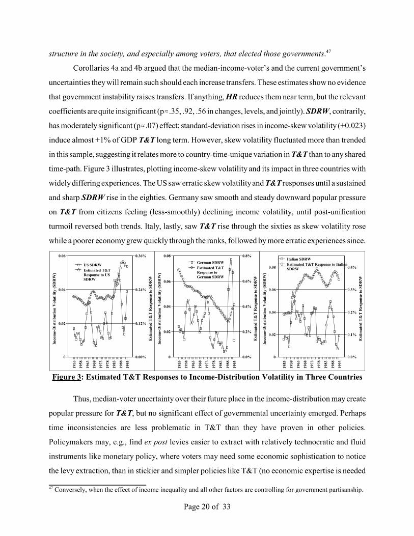
Finally, consider the interactive effects of voter participation, VP, and income skew, RW: the
core of the amended model. The joint significance (p�.05) of RW, VP, and VP����RW establishes that
income skew, voter participation, and/or their interaction affect T&T, broadly supporting Hypotheses
1 and 7. Other tests determine that income skew, by itself and/or interacting with VP, affects T&T
(brw=bvp�rw=0 � p�.045) and the analogous for voter participation (bvp=bvp�rw=0 � p�.02). Finally, the
significant (p�.015) positive coefficient on the interaction term implies that the effects of RW and
of VP on T&T each become less-negative/more-positive as the other variable increases: strong direct
support for Hypothesis 7. Graphics will help interpret the substance of these results since the effects
reflected in the coefficients on interactive terms and the standard errors of those effects depend upon,
and so can only be interpreted as a function of, the levels of each variable (Franzese et al. 1999).
The top-left of Figure 4 plots estimated first-year T&T responses to a 0.1 rise in the societal
income-skew index, as a function of voter-participation rates over their sample range; i.e., it plots
brw+bvp�rwVP, plus an 80% confidence interval (marking one-sided .10 t-tests,48 with countries labeled
on the effect line at their postwar-average VP.49 As seen, governments respond to high income skews
by raising transfers at any VP rate, and more so at higher VP (Hypotheses 1,7). Governments in the
least-participatory democracies, US and Switzerland, respond least�indeed, indistinguishable from
zero statistically�to rising income-skew. Contrarily, government responses to higher income-skews
in the most-participatory democracies, Australia and Austria, are quite statistically and substantively
significant: +0.1 RW induces short-run +.08% and, if permanent, long-run +1.2% of GDP T&T.
50 69% of total RW variation is cross-national.
Page 22 of 33
Uni
ted
Stat
es
Switz
erla
nd
Japa
nSp
ain
Irel
and
Can
ada
Fran
cePo
rtug
alU
nite
d K
ingd
omFi
nlan
dG
reec
e
Nor
way
Ger
man
yD
enm
ark,
Sw
eden
Bel
gium
New
Zea
land
Ital
y, N
ethe
rlan
ds
Aus
tral
iaA
ustr
ia
47 49 51 53 55 57 59 61 63 65 67 69 71 73 75 77 79 81 83 85 87 89 91 93
Voter Participation Rate (%)
-0.05
0.00
0.05
0.10
0.15
As a
Fun
ctio
n of
the
Polit
y's V
oter
Par
ticip
atio
n R
ate
Imm
edia
te T
&T
Impa
ct o
f 0.1
Incr
ease
in In
com
e Sk
ew
TT Impact of 0.1 Increase in RW as a Function of VP: 0.1*[d(TT)/d(RW)]80% Confidence Interval (Critical Values for One-Sided p=0.10 Tests)
Finl
and
Swed
en
Nor
way
Japa
n
Port
ugal
Net
herl
ands
Den
mar
kB
elgi
umC
anad
a
New
Zea
land
Ger
man
ySw
itzer
land
Aus
tral
iaU
nite
d St
ates
Ital
yA
ustr
ia
Uni
ted
Kin
gdom
Irel
and
Fran
ce Spai
n
Gre
ece
0.48
0.51
0.54
0.57
0.60
0.63
0.66
0.69
0.72
0.75
0.78
0.81
0.84
0.87
0.90
0.93
0.96
0.99
1.02
1.05
1.08
1.11
1.14
1.17
1.20
1.23
1.26
1.29
1.32
Index of Income Skew
-0.05
0.00
0.05
0.10
0.15
0.20
Part
icip
atio
n as
a F
unct
ion
of th
e E
cono
my'
s Inc
ome
Skew
Imm
edia
te T
&T
Impa
ct o
f 10%
Incr
ease
in V
oter
TT Impact of 10% Increase in VP as a Function of RW: 0.1*[d(TT)/d(VP)]80% Confidence Interval (Critical Values for One-Sided p=0.10 Tests)
T-2 T0 2 4 6 8 10 12 14 16 18 20 22 24 26 28 30 32 34 36 38 40 42 44 46 48 50
Years Since Voter-Participation Increase (Occurs in T0)
0
0.5
1
1.5
2
in V
oter
Par
ticip
atio
n at
Var
ious
Inco
me-
Skew
Lev
els
Res
pons
e of
T&
T (%
of G
DP)
to a
10%
Incr
ease
T&T Response at RW=0.500 (FI)T&T Response at RW=0.625 (NO/JA)T&T Response at RW=0.750 (BE)
T&T Response at RW=0.875 (US/IT)T&T Response at RW=1.000 (FR)
T&T Response at RW=1.180 (SP)T&T Response at RW=1.310 (GR)
Fin 0.50Swe 0.54Nor 0.62Jap 0.63Port 0.71Neth 0.73Den 0.74Bel 0.75Can 0.76NZ 0.81Ger 0.82Swi 0.82
Austral 0.83US 0.87Ita 0.88
Austria 0.88UK 0.92Ire 0.98Fra 1.00Spa 1.18Gre 1.31
Postwar-AverageIncome-Skew Index
T-2 T0 2 4 6 8 10 12 14 16 18 20 22 24 26 28 30 32 34 36 38 40 42 44 46 48 50
Years Since Income-Disparity Increase (Occurs in T0)
0
0.2
0.4
0.6
0.8
1
1.2
Inco
me-
Skew
Inde
x at
Var
ious
Vot
er-P
artic
ipat
ion
Rat
esR
espo
nse
of T
&T
(% o
f GD
P) to
0.1
Incr
ease
in th
e
T&T Response at VP=0.48 (US)T&T Response at VP=0.58 (Swi)T&T Response at VP=0.72 (Jap)
T&T Response at VP=0.76 (UK)T&T Response at VP=0.81 (Nor)T&T Response at VP=0.85 (Ger)
T&T Response at VP=0.89 (Ita)T&T Response at VP=0.92 (Aus)
US 0.482Swi 0.581Jap 0.715Spa 0.722Ire 0.733
Can 0.737Fra 0.747Por 0.748UK 0.763Fin 0.774Gre 0.792Nor 0.813Ger 0.851Den 0.853Swe 0.857Bel 0.866NZ 0.882Net 0.884Ita 0.885
Austral 0.915Austria 0.922
Postwar-AverageVoter-Participation Rates
Figure 4: Estimated Immediate and Longer-term T&T Response to Increases in Income Skew as a Functionof Voter Participation and to Increases in Voter Participation as a Function of Income Skew
The top-right analogously plots estimated T&T responses to a 10% increase in participation
as a function of income skew, over RW�s sample range, with country labels at their sample-average
RW,50 plus confidence intervals. Voter participation generally raises T&T, as argued before, and this
relation becomes more positive and significant as underlying income-skew increases, as Corollary
7a added. These effects can be appreciable: in the US in 1986 (RW=1), +10% voter-participation
raises T&T .08% of GDP short-run and, if permanent, 1.3% long-run. Thus, the impact of expanding
the politically active population depends on the characteristics of those joining the voting pool.
The bottom of Figure 4 facilitates further substantive interpretation, plotting T&T responses
over time to sustained 10% increases in the income-skew index and in voter-participation rates at
revealing levels of the other variable. For example, the bottom-left plots T&T responses to RW at
US postwar-average VP, .48 (near the sample-minimum of .41); the Swiss average, .58; Japan�s .72,
(a standard deviation below mean); the UK�s .76 and Norway�s .81 (bridging the mean of .79);
Germany�s .85; Italy�s .89 (a standard deviation above mean); and Austria�s .92 (just below the
maximum of .94). The bottom-right plots analogous T&T responses to VP increases at substantively
revealing levels of RW. All countries� postwar-average VP (democratic periods only) and RW are

51 I.e., the general proposition that the effects differ depending on voter-participation rates is statistically significant(bvp�rw=0�p�.016). Whether any two country-times differ significantly will depend on their exact VP rates.
Page 23 of 33
1952
1956
1960
1964
1968
1972
1976
1980
1984
1988
1992
0.7
0.75
0.8
0.85
0.9
0.95
and
Indi
ces o
f Inc
ome-
Dist
ribu
tion
Skew
(RW
)
OE
CD
-Ave
rage
Vot
er-P
artic
ipat
ion
Rat
es (V
P)
2.0%
2.2%
2.4%
2.6%
2.8%
3.0%
Est
imat
ed T
rans
fers
(% o
f GD
P) R
espo
nseVP Average (excluding non-democracies)
RW AverageEstimated T&T Response
Figure 5: Estimated T&T Responses to OECD-Average Paths of Voter Participation and Income Skew
listed, so approximate T&T-responses at any country�s average VP or RW can be visualized.
Figure 4 shows the clear empirical support for Hypothesis 7. Higher underlying income skew
raises popular demand for transfers, but popular demand translates to politically effective demand
at rates depending on participation. The bottom-left shows that where nearly everyone votes, as in
Austria or Australia, e.g., which fine(d) for abstaining, a sustained standard-deviation rise in income
skew, +.22 RW, would lead governments to raise T&T 2.6% of GDP in the long run. Where, instead,
participation lies near its democratic nadir, the US�s average 48%, a sustained 10% income-skew
rise draws only a statistically insignificant and substantively small 0.37% of GDP long-run T&T
response from governments. Conversely, the bottom-right shows a 10% rise in voter-participation
produces a 4.8% of GDP long-run T&T increase at sample-maximum income-skew (1.54 in Greece
1965) and a negligible decrease at sample minimum (.29 in Japan 1956). These differences are
statistically as well as substantively significant.51 Moreover, as Figure 5 shows, OECD-average paths
of VP and RW, slightly downward and erratically upward respectively, yielded net popular pressures
on governments accounting for about 1% of GDP of the common upward T&T time-path, about half
of the cross-country-shared time variation left unexplained by economic conditions alone.
VI. Conclusions
Consider, lastly, the other question raised above: how well can the positive political economy
of tax-and-transfer systems, as expanded here, explain the similarities and differences in the postwar

52 The OECD-average UE path�flat around 2.5% 1955-74, up to 8% by 1983, to under 7% in 1990, back to 10% in1992-3, before ebbing�can account for +1% of GDP T&T 1974-83, -1.2% 1983-90, +.6% 1990-2, and -.5% 1993-6.
Page 24 of 33
T&T experiences of developed democracies? Table 2 begins an answer, giving first-year and long-
run effects of permanent standard-deviation rises in each independent variable. As seen, the factors
with most impact were economic conditions�unemployment, inflation, growth, wealth�plus labor-
organizational strength, electioneering, government partisanship, income volatility, and interactions
of income skew and voter participation. Age-demographics and fiscal complexity may also have
contributed. These factors together can explain almost an adjusted half of the total variation in T&T
experiences depicted in Figure 1. For its part, the OECD-average T&T trend, +14.5% of GDP T&T
1950-93, seems to have stemmed from common growth and wealth developments primarily. OECD-
average real-GDP-per-capita, trending upward at slowing growth rates, accounts for +6% of GDP
T&T, over 40% of total trend, including both growth slow-down and wealth-accumulation effects.
The over-65 age-group, meanwhile, rose 8.75-14.25% of total population 1950-93, which accounts
for another +1.7% of GDP T&T, if its insignificant coefficient estimate (p�.37) is trusted. Other
economic conditions, unemployment and inflation, had smaller long-term effects, but especially UE
sizably impacted shared short-term fluctuations around the trend.52 All told, over half the OECD-
average upward T&T trend and about half the shared fluctuations around that trend are attributable
to fairly automatic responses of existing transfers policies to economic and demographic conditions.

Page 25 of 33
Table 2: Independent Variables� Short-Run and Long-Run Impacts on T&T-Size
Independent Variable Std. Dev.T&T Impact of 1 Std. Dev. Increase in Indep. Var.
Short-Run Long-RunUE 3.5808 0.8013*** -0.7817
POP65 2.4373 0.3368 1.0758CPI 5.1406 -0.1875*** -0.4196����Y 0.0291 -0.2344*** -2.4660***
Y 0.4418 -2.2501*** 2.6615*
OPEN 0.2416 0.0387 0.6439CTAX 0.1402 -0.0299 -0.4971ITAX 0.0907 0.0766 1.2742TTAX 0.0322 0.0034 0.0563UDEN 16.2137 0.1262** 2.1000**
ELE see note 0.2259** 1.1278***
CoG 1.8134 -0.0709* -0.6485HR 0.3231 -0.0326 -0.0567
SDRW 0.0203 0.0504* 0.8390*
VP at RW mean-2sd
0.2168
0.0143 0.2387VP at RW mean-1sd 0.0693 1.1527
VP at RW mean 0.1242 2.0667VP at RW mean+1sd 0.1791** 2.9806**
VP at RW mean+2sd 0.2341*** 3.8946***
RW at VP mean-2sd
0.2226
0.0040 0.0671RW at VP mean-1sd 0.0575 0.9573
RW at VP mean 0.1110* 1.8474*
RW at VP mean+1sd 0.1645** 2.7375**
RW at VP=1 0.1757** 2.9227**
NOTES: Short-run impacts are estimated first-year effects of 1-standard-deviation increases in independent variables.Long-run impacts are estimated long-run effects of permanent 1-standard-deviation increases in independent variables.*=p�.10, **=p�.05, ***=p�.01; two-sided. Short-run impact for ELE combines the two-year T&T-impulses from oneelection; the long-run impact reflects a permanent increase in electoral frequency from every 5 to every 2 years.
Structural-political developments also had strong effects. E.g., labor-organizational strength:
a standard-deviation rise in union density (+16%) induces +2.1% of GDP T&T, a substantively and
statistically significant amount. Voter fiscal illusion and budgetary complexity may also have been
important, with effect magnitude equal to age-demographics if its mildly insignificant coefficient
is trusted. However, unionization and tax-complexity trends, up-then-down and toward simplicity,
worked against the upward T&T trend, pushing up-then-down and down on T&T, ±.25% and -1.4%
of GDP respectively. Election-years, electoral frequency, partisanship, and income-distribution
volatility similarly played key roles in explaining cross-country-average and country-time-unique
variation, but none had much-shared time-path, and so none were central to the shared upward T&T
trend. Voter participation and income skew, contrarily, added strongly to transfers trends in some

53 Table 3 assumes coefficients, which country dummies assure rely solely upon time-variation, will correctly reflect long-run T&T-size differences. Actually, though, all fixed-coefficient time-series-cross-section model assume so.
Page 26 of 33
countries; standard-deviation adverse shifts in either adds +3% of GDP T&T where both were high,
though they were less central in country-times where one or both were low. As Figure 5 showed,
the OECD-average paths of VP and RW actually account for a sizable +1% of GDP average.
Thus, the full political-economic model can explain about half the common upward trend in
transfers (6+1.7+1 -1.4%=7.3% of 14.5%) and also about half the shared fluctuation around it, which
together represent about 46% of total variance in T&T. And the interaction of participation and
inequality stressed here is an important element of that explanation. Moreover, despite failing to
render the atheoretical country-indicators statistically redundant, the model could also explain almost
half the variation across country-averages in T&T, 43±% of the total. Table 3 demonstrates.53
The last few rows of Table 3 show that the key conditions behind cross-country variation in
T&T-size are not transitory macroeconomic conditions like growth, unemployment, and inflation
but more-durable socioeconomic conditions like, especially, aggregate wealth and, also though less-
so, society�s age distribution. Note that such factors foster governments T&T largesse at least partly
through their effects on the polity�s structure of interests. Economic forces, while important, do not
solely drive either the relationship between aggregate wealth and T&T-size or that between age-
demographics and T&T-size. Wealthier and older polities also demand more social transfers from
their governments as a normative luxury (i.e., Wagner�s Law) and because more citizens benefit
directly from public pensions and so work to increase/defend them politically.Table 3: Estimated Long-Run T&T Impacts of Countries� Postwar-Average Political-Economic Conditions
UE
POP
INF
d(Y
)
Y
OPE
N
CTA
X
ITA
X+
TT
AX
UD
EN
EL
E
CoG HR
SDR
W
VPR
W
SUM
Fixe
dE
ffect
NET
T&
T
US -0.7 2.5 -0.2 -0.7 30.1 0.2 -1.0 3.0 1.6 0.5 -1.2 0.0 0.5 0.1 34.8 -29.4 5.4 8.0JA -0.2 2.1 0.0 -2.2 27.7 0.3 -1.0 3.3 2.1 0.8 -1.6 -0.1 0.7 0.4 32.3 -27.4 5.0 7.2GE -0.2 3.2 -0.2 -1.4 28.9 0.5 -0.7 3.3 2.3 0.5 -1.1 0.0 0.6 1.9 37.8 -30.4 7.4 14.2FR -0.2 3.1 -0.2 -1.2 28.8 0.4 -1.0 3.6 1.3 0.5 -1.1 0.0 0.5 2.2 36.7 -26.4 10.2 16.7IT -0.5 2.9 -0.3 -1.4 28.2 0.4 -1.2 3.2 2.3 0.5 -1.0 -0.1 0.6 2.4 35.9 -27.3 8.6 14.5UK -0.4 3.3 -0.3 -0.9 28.8 0.5 -1.4 3.9 2.9 0.5 -1.2 0.0 0.3 1.9 37.9 -32.2 5.6 9.4CA -0.6 2.2 -0.2 -0.9 29.5 0.6 -1.0 3.7 2.1 0.6 -1.0 0.0 0.5 1.0 36.5 -30.5 6.0 9.0AU -0.2 3.3 -0.1 -1.4 28.3 0.6 -1.0 3.7 3.7 0.6 -0.9 0.0 0.4 2.6 39.5 -29.9 9.6 16.4BE -0.4 3.2 -0.2 -1.1 28.6 1.4 -1.2 3.1 3.3 0.7 -1.1 -0.1 0.5 1.5 38.3 -26.1 12.2 18.5DE -0.5 3.1 -0.2 -1.2 29.0 0.7 -1.3 3.8 4.6 0.8 -1.0 -0.1 0.3 1.4 39.5 -31.3 8.2 11.9FI 0.1 2.5 -0.3 -1.2 28.5 0.6 -1.1 3.4 3.6 0.4 -0.9 0.0 0.4 -0.1 35.9 -28.3 7.6 10.2
GR -0.4 2.8 -0.4 -1.5 26.2 0.4 -1.1 4.2 2.4 0.5 -1.4 -0.1 1.4 2.6 35.8 -29.3 6.4 8.9IR -0.8 2.6 -0.3 -1.5 27.2 1.1 -1.6 4.8 3.3 0.6 -1.1 0.0 0.6 2.0 36.8 -30.6 6.3 9.9NE -0.3 2.6 -0.1 -1.2 28.8 1.3 -1.2 2.9 2.2 0.6 -1.0 0.0 0.4 1.5 36.3 -23.0 13.3 17.3NO -0.2 3.2 -0.3 -1.4 28.9 0.8 -1.3 3.6 3.7 0.5 -0.7 0.0 0.4 0.6 37.6 -28.8 8.8 11.5PO -0.3 2.5 -0.4 -1.8 25.8 0.7 -1.2 3.8 4.1 0.3 -1.5 -0.1 0.8 -0.8 32.1 -31.1 1.0 5.5
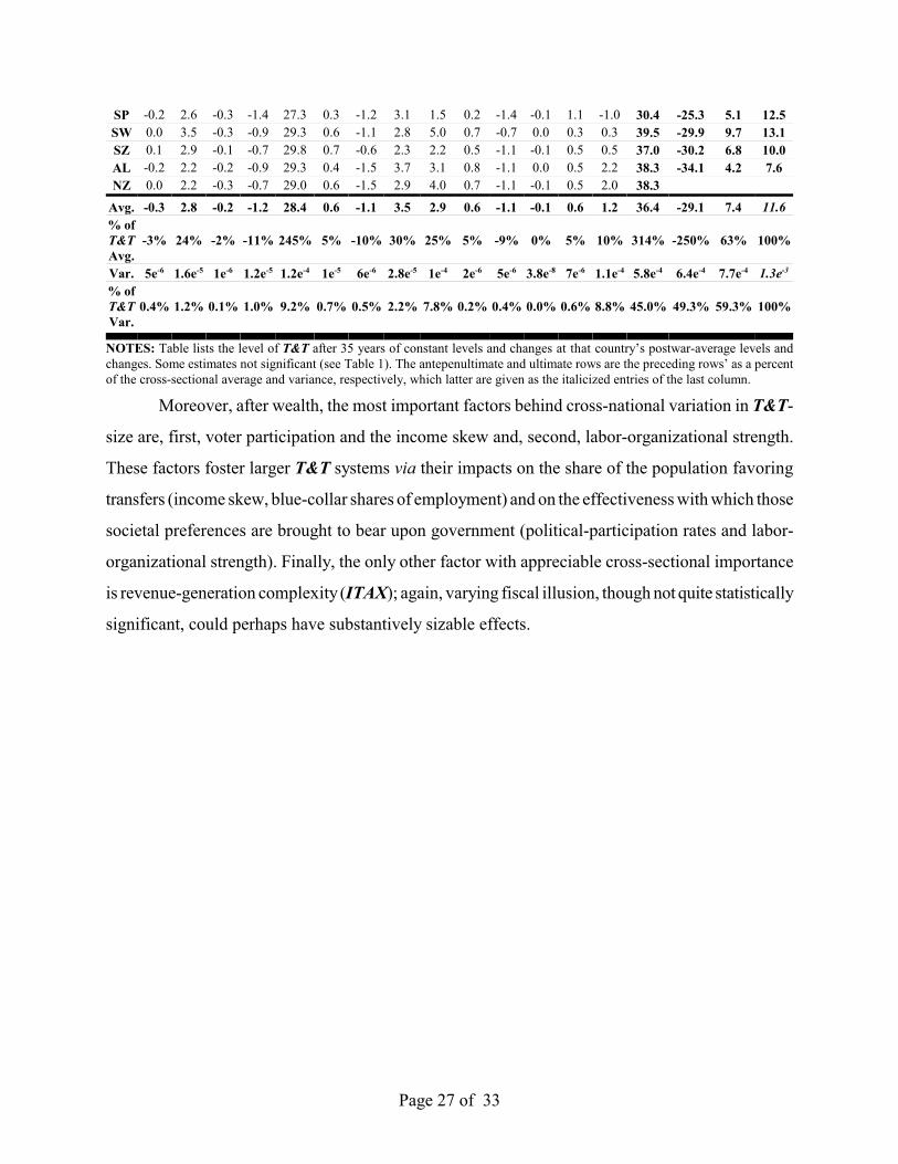
Page 27 of 33
SP -0.2 2.6 -0.3 -1.4 27.3 0.3 -1.2 3.1 1.5 0.2 -1.4 -0.1 1.1 -1.0 30.4 -25.3 5.1 12.5SW 0.0 3.5 -0.3 -0.9 29.3 0.6 -1.1 2.8 5.0 0.7 -0.7 0.0 0.3 0.3 39.5 -29.9 9.7 13.1SZ 0.1 2.9 -0.1 -0.7 29.8 0.7 -0.6 2.3 2.2 0.5 -1.1 -0.1 0.5 0.5 37.0 -30.2 6.8 10.0AL -0.2 2.2 -0.2 -0.9 29.3 0.4 -1.5 3.7 3.1 0.8 -1.1 0.0 0.5 2.2 38.3 -34.1 4.2 7.6NZ 0.0 2.2 -0.3 -0.7 29.0 0.6 -1.5 2.9 4.0 0.7 -1.1 -0.1 0.5 2.0 38.3
Avg. -0.3 2.8 -0.2 -1.2 28.4 0.6 -1.1 3.5 2.9 0.6 -1.1 -0.1 0.6 1.2 36.4 -29.1 7.4 11.6% ofT&TAvg.
-3% 24% -2% -11% 245% 5% -10% 30% 25% 5% -9% 0% 5% 10% 314% -250% 63% 100%
Var. 5e-6 1.6e-5 1e-6 1.2e-5 1.2e-4 1e-5 6e-6 2.8e-5 1e-4 2e-6 5e-6 3.8e-8 7e-6 1.1e-4 5.8e-4 6.4e-4 7.7e-4 1.3e-3
% ofT&TVar.
0.4% 1.2% 0.1% 1.0% 9.2% 0.7% 0.5% 2.2% 7.8% 0.2% 0.4% 0.0% 0.6% 8.8% 45.0% 49.3% 59.3% 100%
NOTES: Table lists the level of T&T after 35 years of constant levels and changes at that country�s postwar-average levels andchanges. Some estimates not significant (see Table 1). The antepenultimate and ultimate rows are the preceding rows� as a percentof the cross-sectional average and variance, respectively, which latter are given as the italicized entries of the last column.
Moreover, after wealth, the most important factors behind cross-national variation in T&T-
size are, first, voter participation and the income skew and, second, labor-organizational strength.
These factors foster larger T&T systems via their impacts on the share of the population favoring
transfers (income skew, blue-collar shares of employment) and on the effectiveness with which those
societal preferences are brought to bear upon government (political-participation rates and labor-
organizational strength). Finally, the only other factor with appreciable cross-sectional importance
is revenue-generation complexity (ITAX); again, varying fiscal illusion, though not quite statistically
significant, could perhaps have substantively sizable effects.
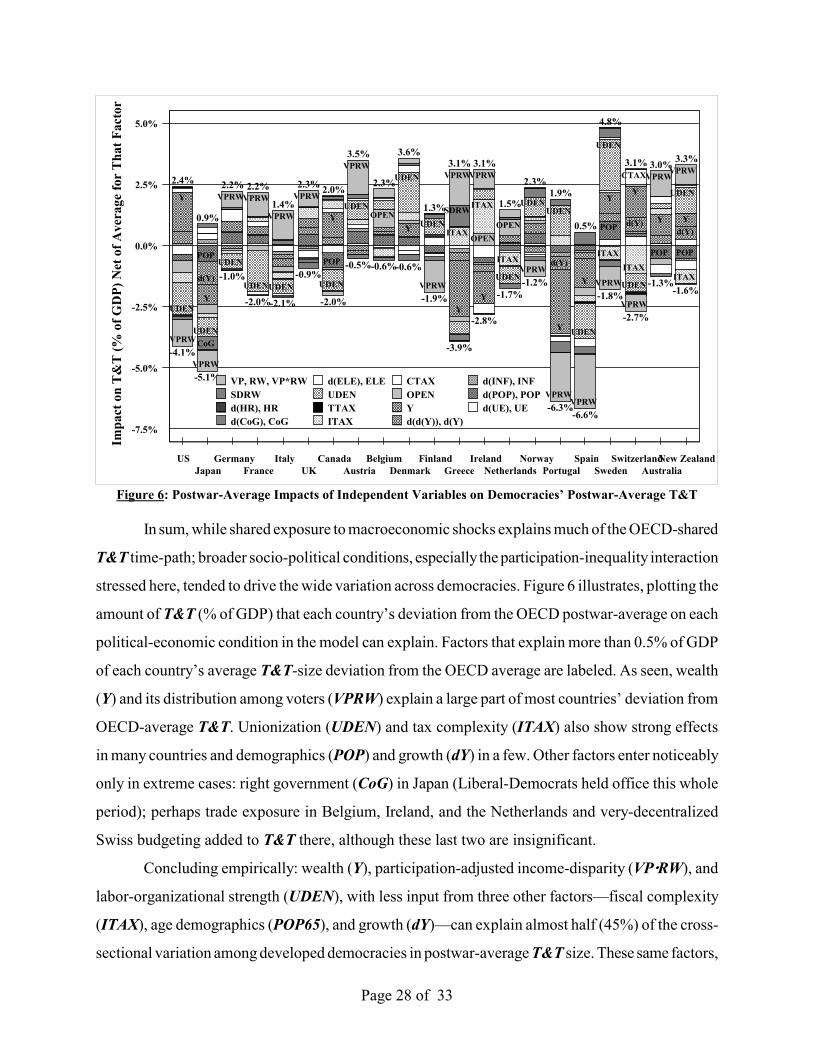
Page 28 of 33
VPRW
VPRW
VPRWVPRW
VPRW
VPRW
VPRW
VPRW
VPRWVPRW
VPRW
VPRWVPRW
VPRW
VPRW
VPRWVPRW
SDRW
CoG
UDEN
UDEN
UDEN
UDENUDEN UDEN
UDEN
UDEN
UDEN
UDEN
UDENUDEN
UDEN
UDEN
UDEN
UDEN
ITAX
ITAX
ITAXITAX
ITAXITAX
CTAX
OPEN
OPENOPEN
Y
Y
YY
YY
Y
Y
YY
Y Y
d(Y)
d(Y)
d(Y)d(Y)
POPPOP
POP
POP POP
-4.1%
2.4%
-5.1%
0.9%
2.2%
-1.0%
2.2%
-2.0%
1.4%
-2.1%
2.3%
-0.9%
-2.0%
2.0%
3.5%
-0.5%
2.3%
-0.6%
3.6%
-0.6%
-1.9%
1.3%
3.1%
-3.9%
3.1%
-2.8%
1.5%
-1.7%-1.2%
2.3%
-6.3%
1.9%
-6.6%
0.5%
-1.8%
4.8%
-2.7%
3.1% 3.0%
-1.3%
3.3%
-1.6%
USJapan
GermanyFrance
ItalyUK
CanadaAustria
BelgiumDenmark
FinlandGreece
IrelandNetherlands
NorwayPortugal
SpainSweden
SwitzerlandAustralia
New Zealand
-7.5%
-5.0%
-2.5%
0.0%
2.5%
5.0%Im
pact
on
T&T
(% o
f GD
P) N
et o
f Ave
rage
for
That
Fac
tor
VP, RW, VP*RWSDRWd(HR), HRd(CoG), CoG
d(ELE), ELEUDENTTAXITAX
CTAXOPENYd(d(Y)), d(Y)
d(INF), INFd(POP), POPd(UE), UE
Figure 6: Postwar-Average Impacts of Independent Variables on Democracies� Postwar-Average T&T
In sum, while shared exposure to macroeconomic shocks explains much of the OECD-shared
T&T time-path; broader socio-political conditions, especially the participation-inequality interaction
stressed here, tended to drive the wide variation across democracies. Figure 6 illustrates, plotting the
amount of T&T (% of GDP) that each country�s deviation from the OECD postwar-average on each
political-economic condition in the model can explain. Factors that explain more than 0.5% of GDP
of each country�s average T&T-size deviation from the OECD average are labeled. As seen, wealth
(Y) and its distribution among voters (VPRW) explain a large part of most countries� deviation from
OECD-average T&T. Unionization (UDEN) and tax complexity (ITAX) also show strong effects
in many countries and demographics (POP) and growth (dY) in a few. Other factors enter noticeably
only in extreme cases: right government (CoG) in Japan (Liberal-Democrats held office this whole
period); perhaps trade exposure in Belgium, Ireland, and the Netherlands and very-decentralized
Swiss budgeting added to T&T there, although these last two are insignificant.
Concluding empirically: wealth (Y), participation-adjusted income-disparity (VP����RW), and
labor-organizational strength (UDEN), with less input from three other factors�fiscal complexity
(ITAX), age demographics (POP65), and growth (dY)�can explain almost half (45%) of the cross-
sectional variation among developed democracies in postwar-average T&T size. These same factors,

54 Some less inspiring results for the basic model also emerged; most notably, its dynamic extension produced nopredictions for T&T systems that were both readily testable and unambiguously passed that test at usual significance.That extension, however, also had other (growth) implications that Alesina and Rodrik (1994) tested successfully.
Page 29 of 33
especially wealth and growth but also the others, plus other economic conditions like unemployment
and inflation, explain also explain almost half the shared time-path of T&T: a 14±% upward trend,
with fluctuations fairly well-explained by macroeconomic conditions. Finally, other considerations,
like election-year politics (ELE), government partisanship (CoG), and income-distribution volatility
(SDRW) also exhibited statistically significant and, in some country-times, substantively large
impacts. These last add to the others in explaining the variation that is unique to particular country-
times. A very rough calculation of the amounts explained might be: 45% of cross-country variation,
which is 43% of the total, explained, plus 50% of the shared time-path, which is 46% of the total,
explained gives approximately 43% of total variation explained so far. The complete model explains
R2=51%, so the model explains 51%-43%=8% more than just accounted, which is fully 85% of the
country-time-unique variation that remains. In other words, the positive political economy of tax-
and-transfers, as extended here, performs moderately well in telling 40-50% of the cross-national
and shared cross-time stories, and especially well in explaining individual country-years� deviations
from their postwar average and the shared time-path, i.e., loosely, at the margins.
Concluding more theoretically, many of the arguments offered here or drawn from previous
literature provide appreciable explanatory leverage, and, in particular, the core prediction of the basic
neoclassical model receives support here as it has not elsewhere.54 Democratic governments do seem
to respond to medians� desires for larger transfers as the income skew rises; however, what matters
theoretically and empirically is the income distribution among the politically relevant subset of the
population. The key point here is that size and composition of that subset (critically, the share and
parts of the income distribution it represents) varies across democracies over time depending on the
interaction of their political (electoral) institutions and economic structure. Specifically, democratic
pressure for redistribution derives from the difference between the median-voter�s income and that
of the population-(tax-payer-) average�s income. Thus, the effective political pressure emanating
from some degree of income disparity in the economy depends on the relative political participation
of different income groups, which, in turn, depends on institutions that foster or hinder turnout
because the relatively well-off vote and otherwise participate effectively everywhere while the less-
well-off participate much more effectively only where they turnout to vote.
Data Appendix: Descriptive Statistics for the T&T Data Set

Page 30 of 33
TT ����(TT) ����(UE) UE ����(POP65) POP65 ����(CPI) CPI UDENMean 12.137 0.286 0.129 4.484 0.137 11.679 0.115 6.556 42.099
Median 11.759 0.186 0.006 3.370 0.149 11.630 0.130 5.010 38.610Maximum 28.332 3.885 4.166 20.940 1.414 18.282 17.610 29.300 84.600Minimum 2.710 -2.168 -2.403 0.002 -0.725 5.641 -13.530 -0.800 9.867Std. Dev. 5.163 0.661 0.820 3.581 0.151 2.437 2.878 5.141 16.214
����(����(Y)) ����(Y) Y OPEN CTAX ITAX TTAX ����(ELE) ELEMean -0.001 0.029 9.040 0.452 0.599 0.354 0.906 -0.001 0.282
Median -0.002 0.029 9.139 0.406 0.601 0.357 0.906 0.000 0.115Maximum 0.122 0.126 9.803 1.396 0.863 0.714 1.000 1.552 1.711Minimum -0.116 -0.105 7.601 0.068 0.263 0.147 0.796 -1.580 0.000Std. Dev. 0.033 0.029 0.442 0.242 0.140 0.091 0.032 0.501 0.337
����(CoG) CoG ����(HR) HR SDRW VP RW VP����RWMean -0.020 5.821 -0.005 0.510 0.026 0.738 0.827 0.593
Median 0.000 5.607 0.000 0.376 0.020 0.795 0.814 0.628Maximum 5.000 10.000 1.279 2.363 0.146 0.943 1.801 1.254Minimum -6.948 2.785 -1.656 0.195 0.002 0.000 0.291 0.000Std. Dev. 0.797 1.813 0.225 0.323 0.020 0.217 0.223 0.211
References
Aldrich, J. 1995. Why Parties? the Origin and Transformation of Political Parties in America, Chpt.6: 182ff. Chicago: The University of Chicago Press.
Aldrich, J. 1983a. �A Downsian Spatial Model with Party Activism,� American Political ScienceReview 77: 1974-90.
Aldrich, J. 1983b. �A Spatial Model with Party Activists: Implications for Electoral Dynamics,�Public Choice 41: 63-100.
Aldrich, J. and M. McGinnis. 1989. �A Model of Party Constraints on Candidate Positions,�Mathematical and Computer Modeling 12: 437-50.
Alesina, A. and D. Rodrik. 1994. �Distributive Politics and Economic Growth,� Quarterly Journalof Economics, 109(2): 465-90.
Alvarez, R.M., G. Garrett, and P. Lange. 1991. �Government Partisanship, Labor Organization, andMacroeconomic Performance,� American Political Science Review 85: 539-56.
Beck, N. 1992. �Comparing Dynamic Specifications: The Case of Presidential Approval,� PoliticalAnalysis 3: 51-87.
Beck, N. And J. Katz. 1998. �Nuisance or Substance: Specifying and Estimating Time-Series-Cross-Section Models,� Political Analysis, 6.
Beck, N. and J. Katz. 1995. �What To Do (and Not to Do) with Time-Series-Cross-Section Data inComparative Politics,� American Political Science Review 89(3): 634-47.
Buchanan, J. and R. Wagner. 1977. Democracy in Deficit, New York: Academic Press.
Cameron, D. 1978. �The Expansion of the Public Economy: A Comparative Analysis,� American

Page 31 of 33
Political Science Review, 72: 1243-61.
Cameron and McDermott. 1995. �Expansion and Contraction of the Public Economy,� unpublished.
Castles, F. (ed.) 1982. The Impact of Parties. London: Sage.
Downs, A. 1957. An Economic Theory of Democracy. New York: Harper and Row.
Downs, A. 1960. �Why the Government�s Budget is Too Small in a Democracy,� World Politics12:541-63
Esping-Andersen, G. 1985. Politics Against Markets. Princeton: Princeton UP.
Esping-Andersen. 1990. The Three Worlds of Welfare Capitalism. Princeton: Princeton UP.
Esping-Andersen, G. 1982. �The Incompatibilities of the Welfare State,� Working Papers for a NewSociety, January, as quoted in Offe 1984, 199.
Franzese, R. 1996a. �A Gauss Procedure to Estimate Panel-Corrected Standard-Errors with Non-Rectangular and/or Missing Data,� The Political Methodologist 7(2):2-3.
Franzese, R. 1996b. The Political Economy of Over-Commitment: A Comparative Study ofDemocratic Management of the Keynesian Welfare State. Cambridge, MA: Ph.D. Thesis,Department of Government, Harvard University.
Franzese, R. 1999. �Partially Autonomous Central Banks, Politically Responsive Governments, andInflation,� American Journal of Political Science XXXX.
Franzese, R. 2000. The Political Economy of Economic Policy in Developed Democracies.Cambridge UP, forthcoming.
Freeman, J., D. Houser, P. Kellstedt, and J.T. Williams. 1996. �Unit Roots and Causal Inference inPolitical Science,� Paper Presented at the 1996 Meeting of the Political Methodology Sectionof the American Political Science Association in Ann Arbor, Michigan.
Garrett, G. 1995. �Capital Mobility, Trade, and the Domestic Politics of Economic Policy,�International Organization 49(4):657-87.
Garrett, G. 1998a. Partisan Politics in the Global Economy. Cambridge: Cambridge UP
Garrett, G. 1998b. �Global Markets and National Politics: Collision Course or Virtuous Circle,�International Organization 52(4).
Golden, M.. P. Lange, and M. Wallerstein. 1995. �Trade Union Organization and IndustrialRelations in the Post-War Era in 16 Nations,� Paper given at the 1995 MidWest PSA.
Harrop, M. and W. Miller. 1987. Elections and Voters: A Comparative Introduction. London:MacMillan.
Hibbs, D. 1977. �Political Parties and Macroeconomic Policy,� American Political Science Review,71: 1467-87.
Hicks, A. 1994. �Introduction to Pooling� in Janoski and Hicks, (eds.), The Comparative PoliticalEconomy of the Welfare State.
Hicks, A., D. Swank, and Ambuhl. 1989. �Welfare Expansion Revisited,� European Journal ofPolitical Research.

Page 32 of 33
Katzenstein, P. 1985. Small States in World Markets. Ithaca: Cornell UP.
Korpi, W. 1980. �Social Policy and Distributional Conflict in the Capitalist Democracies,� WestEuropean Politics, 3.
Korpi, W. 1983. The Democratic Class Struggle. London: Routledge and Kegan Paul.
Kreps, D. 1990. �Corporate Culture and Economic Theory,� in J. Alt and K. Shepsle (eds.),Perspectives on Positive Political Economy, Cambridge: Cambridge UP.
Kydland, F.E. and E.C. Prescott. 1977. �Rules Rather than Discretion: The Inconsistency of OptimalPlans,� Journal of Political Economy 85: 473-92.
Lane, J-E., D. McKay, and K. Newton. 1991. Political Data Handbook: OECD Countries, NewYork: Oxford UP.
Laver, M. and W. Hunt. 1992. Policy and Party Competition, New York: Routledge, Chapman, andHall, Inc.
Laver, M. and Schofield. 1991. Multiparty Government: The Politics of Coalition in Europe, NewYork: Oxford UP.
Mackie, T. and R. Rose. 1991. The International Almanac of Electoral History. DC: CongressionalQuarterly.
Meltzer, A. and S. Richard. 1978. �Why Government Grows (and Grows) in a Democracy,� ThePublic Interest, 52: 111-8.
Meltzer, A. and S. Richard. 1981. �A Rational Theory of the Size of Government,� Journal ofPolitical Economy 89(5):914-27.
Moene, K.O. and M. Wallerstein. 1999. �Inequality, Social Insurance, and Redistribution,�unpublished, University of Oslo and Northwestern University.
OECD. 1995. Social Policy Studies #18: Income Distribution in OECD Countries. Paris: OECD.
Offe, C. 1984. Contradictions of the Welfare State. London: Hutchinson.
Olson, M. 1965, The Logic of Collective Action: Public Goods and the Theory of Groups.Cambridge: Harvard UP.
Pampel, F. and J. Williamson. 1988. �Welfare Spending in Advanced Industrial Democracies 1950-1980,� American Journal of Sociology, 93(6): 1424-56.
Peterson, P.E. 1990. Welfare Magnets: A New Case for a National Standard (Washington, D.C.:Brookings Institution).
Rodrigìuez, F.C. 1999. �Does Distributional Skewness Lead to Redistribution? Evidence from theUnited States,� Economics and Politics, 11(2): 171-99.
Romer, T. 1975. �Individual Welfare, Majority Voting, and the Properties of a Linear Income Tax,�Journal of Public Economics, 14: 163-85.
Romer, T. and H. Rosenthal. 1978. �Political Resource Allocation,� Public Choice.
Rosenstone, S.J. and J.M. Hansen. 1993. Mobilization, Participation, and Democracy in America.New York: MacMillan.

Page 33 of 33
Schultz, K. 1995. �The Politics of the Political Business Cycle,� British Journal of Political Science,25(1): 79-100.
Sharpe, . 1988. �The Growth and Decentralization of the Modern Democratic State,� EuropeanJournal of Political Research, .
Tufte, E. 1978. Political Control of the Economy. Princeton: Princeton UP.
Verba, S., N.H. Nie, and J. Kim. 1978. Participation and Political Equality: A Seven-NationComparison. Chicago: The University of Chicago Press.
Verba, S., K.L. Schlozman, and H.E. Brady. 1995. Voice and Equality: Civic Voluntarism inAmerican Politics. Cambridge: Harvard UP.
Weingast, B., K. Shepsle, and C. Johnsen. 1981. �The Political Economy of Costs and Benefits,�Journal of Political Economy, 89: 642-64.
Wilensky, H. 1975. The Welfare State and Equality. Berkeley: The University of California Press.
Wilensky, H. 1981. �Leftism, Catholicism, and Democratic Corporatism,� in P. Flora and A.Heidenheimer (eds.), The Development of Welfare States in Europe and America. London:Transaction Books.
Woldendorp, J., H. Keman, and I. Budge. 1994. �Party Government in 20 Democracies,� EuropeanJournal of Political Research, (Special Issue: Political Data 1945-90), 24(1).
Wolfinger, R.E and S.J. Rosenstone. 1980. Who Votes? New Haven : Yale UP.
Top Related