


Languages
Pages
Legal


Plastic Deformation and Ductile Fracture of Ti-6Al-4V under
Various Loading Conditions
THESIS
Presented in Partial Fulfillment of the Requirements for the DegreeMaster of Science in the Graduate School of The Ohio State
University
By
Jeremiah Thomas Hammer, B.S.
Graduate Program in Mechanical Engineering
The Ohio State University
2012
Master’s Examination Committee:
Dr. Amos Gilat, Advisor
Dr. Mark Walter

c© Copyright by
Jeremiah Thomas Hammer
2012
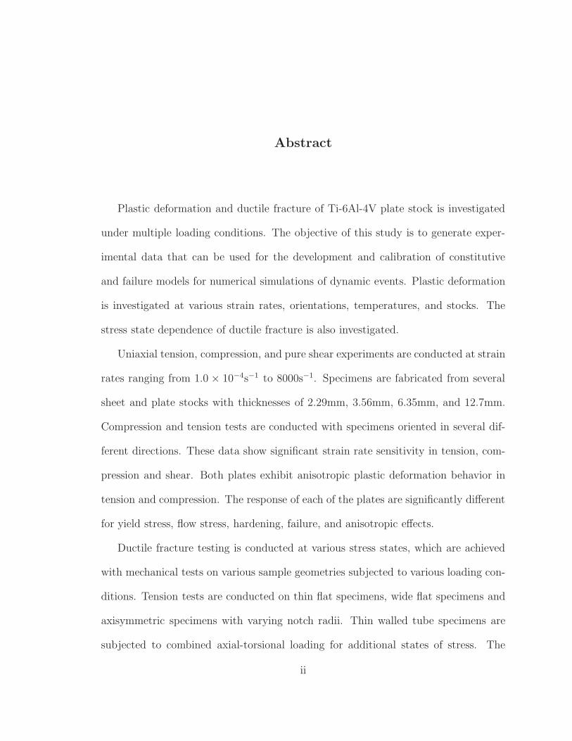
Abstract
Plastic deformation and ductile fracture of Ti-6Al-4V plate stock is investigated
under multiple loading conditions. The objective of this study is to generate exper-
imental data that can be used for the development and calibration of constitutive
and failure models for numerical simulations of dynamic events. Plastic deformation
is investigated at various strain rates, orientations, temperatures, and stocks. The
stress state dependence of ductile fracture is also investigated.
Uniaxial tension, compression, and pure shear experiments are conducted at strain
rates ranging from 1.0 × 10⁻⁴s−1 to 8000s−1. Specimens are fabricated from several
sheet and plate stocks with thicknesses of 2.29mm, 3.56mm, 6.35mm, and 12.7mm.
Compression and tension tests are conducted with specimens oriented in several dif-
ferent directions. These data show significant strain rate sensitivity in tension, com-
pression and shear. Both plates exhibit anisotropic plastic deformation behavior in
tension and compression. The response of each of the plates are significantly different
for yield stress, flow stress, hardening, failure, and anisotropic effects.
Ductile fracture testing is conducted at various stress states, which are achieved
with mechanical tests on various sample geometries subjected to various loading con-
ditions. Tension tests are conducted on thin flat specimens, wide flat specimens and
axisymmetric specimens with varying notch radii. Thin walled tube specimens are
subjected to combined axial-torsional loading for additional states of stress. The
ii
results show that the stress triaxiality alone is unable to properly capture the fail-
ure characteristics of material. Digital image correlation is used to measure surface
strains of the specimens. Parallel LS-DYNA simulations are used to determine the
stress states and fracture strains. A fracture locus for Ti-6Al-4V is created in the
stress triaxiality and Lode parameter stress space giving a more accurate description
of the material fracture.
An experimental technique is introduced to measure full field strains using three
dimensional digital image correlation at temperatures up to 800C. This test setup
has been designed to be a straight forward, repeatable, and accurate method for
measuring strains at high temperatures. Design hurdles included thermal gradients of
air, speckle pattern adhesion, viewing window image distortion, camera calibration,
and infrared light pollution of the camera sensor. For validation, the coefficient
of thermal expansion for Ti-6Al-4V up to 800C is measured using the technique
and compared to published values. Tests on Ti-6Al-4V were conducted in tension,
compression, and torsion (shear). Experimentally measured coefficient of thermal
expansion values correlate well with handbook values. The system performs well for
each of the tests conducted here and gives substantially more data than standard
methods.
iii

This document is dedicated to my family and close friends.
iv

Acknowledgments
Many people have helped me get to this point in my life and I would like to
thank them. First and foremost I would like to thank my parents Bonnie and Peter
Hammer, without their love and support through both smooth and rough times I
do not think this would have been possible. Josh and Mary Moran have also been
a constant source of support and friendship. There are countless other friends that
have also been a source of inspiration.
My Advisor, Professor Amos Gilat, has been both inspiring and supportive. His
advice during my time here has been invaluable and it has been a true pleasure to
work with him. Dr. Jeremy Seidt has become a mentor both in and out of the
laboratory as well as an esteemed colleague. During my time working on this project
Jeremy has become a second advisor and I do not think the project would have had
the same results without his guidance. Thanks also to Professor Mark Walter as my
thesis defense committee member.
This research was funded by the Federal Aviation Administration with collabora-
tion from National Aeronautics and Space Administration as well as George Wash-
ington University. Thanks to Don Altobelli, Bill Emmerling, and Chip Queitzsch
from the FAA for all the support given to myself during this project. Thanks also to
Paul Dubois, Steve Kan, and Doug Wang.
v

Thanks to Mike Pereira, Adam Howard, Kelly Carney, Chuck Ruggeri, and Brad
Lerch of NASA Glenn Research Center for their support both during my master’s
research and my time spent at the Glenn Research Center.
Thanks also to Casey Holycross, Matti Isakov, Bob Lowe, Chris Cooley, Tom
Matrka, Kevin Gardner, Emily Sequin, Zach Witeof, Mark Ryan, Michelle Wilson,
Jarrod Smith, and Tim Liutkus. These students and researchers in the Mechanical
and Aerospace Engineering Department at The Ohio State University have helped
immensely with both technical discussions regarding the research and the friendship
they provided. I also want to thank my friends and colleagues of Pi Tau Sigma.
vi

Vita
2000 . . . . . . . . . . . . . . . . . . . . . . . . . . . . . . . . . . . . . . . .Frederick High School, Frederick, MD
2010 . . . . . . . . . . . . . . . . . . . . . . . . . . . . . . . . . . . . . . . .B.S. Mechanical Engineering,The Ohio State University
2010-present . . . . . . . . . . . . . . . . . . . . . . . . . . . . . . . .Graduate Research Associate,Dynamic Mechanics of MaterialsLaboratory,Department of Mechanical andAerospace Engineering,The Ohio State University
Publications:
Seidt, J.D. Pereira, J.M., Hammer, J.T., Gilat, A., “Dynamic Load Measurementof Ballistic Gelatin Impact Using an Instrumented Tube”, Proceedings of the 2012
SEM Annual Conference and Exposition on Experimental and Applied Mechanics,Costa Mesa, CA, June, 2012
Hammer, J.T., Yatnalkar, R.S., Seidt, J.D., Gilat, A., “Plastic Deformation of Ti-6Al-4V Plate over a Wide Range of Loading Conditions”, Proceedings of the 2012
SEM Annual Conference and Exposition on Experimental and Applied Mechanics,Costa Mesa, CA, June, 2012
Hammer, J.T., Seidt, J.D., Gilat, A., “Strain Measurement at Temperatures up to
800C Utilizing Digital Image Correlation”, Proceedings of the 2013 SEM AnnualConference and Exposition on Experimental and Applied Mechanics, Lombard, IL,
June, 2013
Hammer, J.T., Seidt, J.D., Gilat, A., “Stress State Dependence on the Ductile Frac-ture of Ti-6Al-4V”, Proceedings of the 2013 SEM Annual Conference and Exposition
on Experimental and Applied Mechanics, Lombard, IL, June, 2013
vii

Howard, S.A., Hammer, J.T., Pereira, J.M., Carney, K.S., “Jet Engine Bird Ingestion
Simulations: Comparison of Rotating to Non-Rotating Fan Blades”, ASME TurboExpo 2013, San Antonio, TX, June, 2013
Fields of Study
Major Field: Mechanical Engineering, Experimental Mechanics, Dynamic Behaviorof Materials, Plasticity, Computational Mechanics
viii

Table of Contents
Page
Abstract . . . . . . . . . . . . . . . . . . . . . . . . . . . . . . . . . . . . . . . ii
Dedication . . . . . . . . . . . . . . . . . . . . . . . . . . . . . . . . . . . . . . iv
Acknowledgments . . . . . . . . . . . . . . . . . . . . . . . . . . . . . . . . . . v
Vita . . . . . . . . . . . . . . . . . . . . . . . . . . . . . . . . . . . . . . . . . vii
List of Tables . . . . . . . . . . . . . . . . . . . . . . . . . . . . . . . . . . . . xiv
List of Figures . . . . . . . . . . . . . . . . . . . . . . . . . . . . . . . . . . . xv
1. Introduction . . . . . . . . . . . . . . . . . . . . . . . . . . . . . . . . . . 1
1.1 Motivation and Objectives for this Research Project . . . . . . . . 4
1.2 Literature Review . . . . . . . . . . . . . . . . . . . . . . . . . . . 91.2.1 Plastic Deformation Behavior of Ti-6Al-4V . . . . . . . . . 10
1.2.2 Ductile Fracture . . . . . . . . . . . . . . . . . . . . . . . . 12
2. Experimental Procedures and Techniques . . . . . . . . . . . . . . . . . . 15
2.1 Introduction . . . . . . . . . . . . . . . . . . . . . . . . . . . . . . 15
2.2 Plastic Deformation of Ti-6Al-4V . . . . . . . . . . . . . . . . . . . 162.2.1 Tension Experiments . . . . . . . . . . . . . . . . . . . . . . 20
2.2.2 Compression Experiments . . . . . . . . . . . . . . . . . . . 212.2.3 Shear Experiments . . . . . . . . . . . . . . . . . . . . . . . 22
2.2.4 Comparison of the Results from the Plastic Deformation Test-ing . . . . . . . . . . . . . . . . . . . . . . . . . . . . . . . . 24
2.3 Ductile Fracture of Ti-6Al-4V . . . . . . . . . . . . . . . . . . . . . 252.3.1 Plane Stress Fracture Testing . . . . . . . . . . . . . . . . . 29
2.3.2 Plane Strain Fracture Testing . . . . . . . . . . . . . . . . . 31
ix

2.3.3 Axisymmetric Fracture Testing . . . . . . . . . . . . . . . . 342.3.4 Combined Loading Testing . . . . . . . . . . . . . . . . . . 38
2.3.5 Fracture Parameter Determination . . . . . . . . . . . . . . 412.4 Quasi-static Strain Rate Testing Techniques . . . . . . . . . . . . . 44
2.5 High Strain Rate Testing Techniques . . . . . . . . . . . . . . . . . 482.5.1 High Strain Rate Compression Testing . . . . . . . . . . . . 48
2.5.2 High Strain Rate Tension Testing . . . . . . . . . . . . . . . 532.5.3 High Strain Rate Shear Testing . . . . . . . . . . . . . . . . 59
2.6 Elevated and Low Temperature Testing Techniques . . . . . . . . . 642.7 Digital Image Correlation . . . . . . . . . . . . . . . . . . . . . . . 67
3. Plastic Deformation of Ti-6Al-4V Experimental Results and Discussion . 71
3.1 Experimental Results from the 2.29mm Plate Stock . . . . . . . . . 71
3.1.1 Strain Rate Test Series Results . . . . . . . . . . . . . . . . 723.1.2 Specimen Orientation Test Series Results . . . . . . . . . . 73
3.2 Experimental Results from the 3.56mm Plate Stock . . . . . . . . . 743.2.1 Strain Rate Test Series Results . . . . . . . . . . . . . . . . 74
3.2.2 Specimen Orientation Test Series Results . . . . . . . . . . 753.3 Experimental Results from the 6.35mm Plate Stock . . . . . . . . . 76
3.3.1 Temperature Test Series Results . . . . . . . . . . . . . . . 763.4 Experimental Results from the 12.7mm Plate Stock . . . . . . . . . 77
3.4.1 Strain Rate Test Series Results . . . . . . . . . . . . . . . . 783.4.2 Specimen Orientation Test Series Results . . . . . . . . . . 80
3.4.3 Temperature Test Series Results . . . . . . . . . . . . . . . 813.5 Comparison of the Various Plate Stocks Tested . . . . . . . . . . . 83
3.5.1 Tension Comparison . . . . . . . . . . . . . . . . . . . . . . 83
3.5.2 Compression Comparison . . . . . . . . . . . . . . . . . . . 883.6 Johnson-Cook Plasticity Model Parameter Determination . . . . . 92
3.7 Yield Criterion . . . . . . . . . . . . . . . . . . . . . . . . . . . . . 963.8 Conclusions . . . . . . . . . . . . . . . . . . . . . . . . . . . . . . . 97
4. Ductile Fracture Experimental Results and Construction of the Fracture
Locus for Ti-6Al-4V . . . . . . . . . . . . . . . . . . . . . . . . . . . . . 100
4.1 Plane Stress Experiments . . . . . . . . . . . . . . . . . . . . . . . 100
4.2 Axisymmetric Experiments . . . . . . . . . . . . . . . . . . . . . . 1014.3 Plane Strain Experiments . . . . . . . . . . . . . . . . . . . . . . . 102
4.4 Combined Loading Experiments . . . . . . . . . . . . . . . . . . . . 1044.5 Fracture Point Determination and Locus Creation . . . . . . . . . . 106
4.6 Johnson-Cook Fracture Parameter Determination . . . . . . . . . . 1114.7 Conclusions for the Ti-6Al-4V Fracture Testing . . . . . . . . . . . 115
x

5. Summary and Conclusions of the Ti-6Al-4V Testing . . . . . . . . . . . . 117
5.1 Plastic Deformation Experimental Conclusions . . . . . . . . . . . 1175.2 Ductile Fracture Experimental Conclusions . . . . . . . . . . . . . 119
5.3 Overall Project Conclusions . . . . . . . . . . . . . . . . . . . . . . 121
6. Strain Measurements at Temperatures up to 800C utilizing Digital ImageCorrelation . . . . . . . . . . . . . . . . . . . . . . . . . . . . . . . . . . 122
6.1 Introduction . . . . . . . . . . . . . . . . . . . . . . . . . . . . . . 1226.1.1 Literature Review . . . . . . . . . . . . . . . . . . . . . . . 123
6.2 Experimental Setup . . . . . . . . . . . . . . . . . . . . . . . . . . 125
6.3 Validation of Measurement System . . . . . . . . . . . . . . . . . . 1296.3.1 Optical Validation . . . . . . . . . . . . . . . . . . . . . . . 129
6.3.2 Coefficient of Thermal Expansion Validation Testing . . . . 1296.4 Experimental Methods and Results of the Various Loading Condi-
tions at High-temperatures . . . . . . . . . . . . . . . . . . . . . . 1336.4.1 Tension Measurement Techniques and Results . . . . . . . . 133
6.4.2 Compression Measurement Techniques and Results . . . . . 1376.4.3 Torsion Measurement Techniques and Results . . . . . . . . 140
6.5 Summary and Conclusions . . . . . . . . . . . . . . . . . . . . . . . 143
Appendices 144
A. Experimental Results from the Ti-6Al-4V Plastic Deformation Test Series 144
A.1 Tension Test Series . . . . . . . . . . . . . . . . . . . . . . . . . . . 145
A.1.1 Tension Strain Rate Dependent Test Series for the 2.29mm
Plate Stock . . . . . . . . . . . . . . . . . . . . . . . . . . . 145A.1.2 Tension Orientation Dependent Test Series for the 2.29mm
Plate Stock . . . . . . . . . . . . . . . . . . . . . . . . . . . 146A.1.3 Tension Strain Rate Dependent Test Series for the 3.56mm
Plate Stock . . . . . . . . . . . . . . . . . . . . . . . . . . . 147A.1.4 Tension Orientation Dependent Test Series for the 3.56mm
Plate Stock . . . . . . . . . . . . . . . . . . . . . . . . . . . 148A.1.5 Tension Temperature Dependent Test Series for the 6.35mm
Plate Stock . . . . . . . . . . . . . . . . . . . . . . . . . . . 149A.1.6 Tension Strain Rate Dependent Test Series for the 12.7mm
Plate Stock . . . . . . . . . . . . . . . . . . . . . . . . . . . 151
xi

A.1.7 Tension Orientation Dependent Test Series for the 12.7mmPlate Stock . . . . . . . . . . . . . . . . . . . . . . . . . . . 153
A.1.8 Tension Temperature Dependent Test Series for the 12.7mmPlate Stock . . . . . . . . . . . . . . . . . . . . . . . . . . . 155
A.2 Compression Test Series . . . . . . . . . . . . . . . . . . . . . . . . 157A.2.1 Compression Strain Rate Dependent Test Series for the 2.29mm
Plate Stock . . . . . . . . . . . . . . . . . . . . . . . . . . . 157A.2.2 Compression Strain Rate Dependent Test Series for the 3.56mm
Plate Stock . . . . . . . . . . . . . . . . . . . . . . . . . . . 158A.2.3 Compression Temperature Dependent Test Series for the 6.35mm
Plate Stock . . . . . . . . . . . . . . . . . . . . . . . . . . . 159A.2.4 Compression Strain Rate Dependent Test Series for the 12.7mm
Plate Stock . . . . . . . . . . . . . . . . . . . . . . . . . . . 159
A.2.5 Compression Orientation Dependent Test Series for the 12.7mmPlate Stock . . . . . . . . . . . . . . . . . . . . . . . . . . . 162
A.2.6 Compression Temperature Dependent Test Series for the 12.7mmPlate Stock . . . . . . . . . . . . . . . . . . . . . . . . . . . 164
A.2.7 Compression Additional for the 12.7mm Plate Stock . . . . 166A.3 Shear Test Series . . . . . . . . . . . . . . . . . . . . . . . . . . . . 167
A.3.1 Shear Strain Rate Dependent Test Series for the 12.7mmPlate Stock . . . . . . . . . . . . . . . . . . . . . . . . . . . 167
A.3.2 Shear Temperature Dependent Test Series for the 12.7mmPlate Stock . . . . . . . . . . . . . . . . . . . . . . . . . . . 170
B. Experimental Results from the Ti-6Al-4V Ductile Fracture Test Series . . 172
B.1 Plane Stress Test Series . . . . . . . . . . . . . . . . . . . . . . . . 173
B.2 Axisymmetric Test Series . . . . . . . . . . . . . . . . . . . . . . . 174B.3 Plane Strain Test Series . . . . . . . . . . . . . . . . . . . . . . . . 177
B.4 Combined Loading Test Series . . . . . . . . . . . . . . . . . . . . . 179
C. Finite Element Meshes used in the Tension Specimen Design for the Frac-ture Characterization Test Series . . . . . . . . . . . . . . . . . . . . . . 183
C.1 Plane Stress Test Series . . . . . . . . . . . . . . . . . . . . . . . . 184C.2 Axisymmetric Test Series . . . . . . . . . . . . . . . . . . . . . . . 186
C.3 Plane Strain Test Series . . . . . . . . . . . . . . . . . . . . . . . . 189
D. Comparison of Experimental Data and Simulations of Fracture Test Series 191
D.1 Plane Stress Test Series . . . . . . . . . . . . . . . . . . . . . . . . 192
D.2 Axisymmetric Test Series . . . . . . . . . . . . . . . . . . . . . . . 196
xii

D.3 Plane Strain Test Series . . . . . . . . . . . . . . . . . . . . . . . . 202D.4 Combined Loading Test Series . . . . . . . . . . . . . . . . . . . . . 205
E. Additional Views of the Fracture Locus for Ti-6Al-4V . . . . . . . . . . . 209
Bibliography . . . . . . . . . . . . . . . . . . . . . . . . . . . . . . . . . . . . 212
xiii

List of Tables
Table Page
1.1 Material composition of the various plate stocks tested . . . . . . . . 8
1.2 Johnson-Cook constitutive parameters for Ti-6Al-4V . . . . . . . . . 11
2.1 Experimental outline for the plastic deformation testing of Ti-6Al-4V 17
2.2 Experimental outline for the plane stress fracture testing . . . . . . . 30
2.3 Experimental outline for the plane strain fracture testing . . . . . . . 33
2.4 Experimental outline for the axisymmetric fracture testing . . . . . . 37
2.5 Experimental outline for the combined loading fracture testing . . . . 40
4.1 Results of the ductile fracture of Ti-6Al-4V testing . . . . . . . . . . 109
4.2 Comparison of Ti-6Al-4V Johnson-Cook constitutive parameters foundin the literature to those determined for plate 4 . . . . . . . . . . . . 116
xiv

List of Figures
Figure Page
1.1 Uncontained engine debris incidents (a)MD-88 Flight 1288 compressor
fan disk failure and subsequent fuselage damage, (b)Fan blade fail-ure from United Airlines Flight 232 incident, (c)Damage to GE-CF6
turbofan engine following disk failure from American Airlines Flight767, (d)Fuselage damage following disk failure from American Airlines
Flight 767 . . . . . . . . . . . . . . . . . . . . . . . . . . . . . . . . . 5
1.2 Virtual and physical testing of blade-off events for turbofan engines
(a)Finite element mesh of a turbofan engine, (b)Finite element resultsof a turbofan engine under loading, (c)Experimental testing of a catas-
trophic blade-off event . . . . . . . . . . . . . . . . . . . . . . . . . . 7
2.1 Specimen manufacturing orientation for the 2.29mm, 3.56mm, and6.35mm plate stocks . . . . . . . . . . . . . . . . . . . . . . . . . . . 18
2.2 Specimen manufacturing orientations for the 12.7mm plate stock . . . 19
2.3 Plane stress smooth specimen used in plastic deformation testing . . 20
2.4 Compression specimen used in plastic deformation testing . . . . . . . 21
2.5 Torsion specimen used in plastic deformation testing . . . . . . . . . 22
2.6 Geometric representation of the shear stress calculation . . . . . . . . 23
2.7 Comparison of stress strain calculation types for the different loadingconditions . . . . . . . . . . . . . . . . . . . . . . . . . . . . . . . . . 25
2.8 Fracture specimen manufacturing orientations for the 12.7mm plate
stock . . . . . . . . . . . . . . . . . . . . . . . . . . . . . . . . . . . . 26
xv

2.9 Points of interest for: (a)plane stress, (b)axisymmetric and (c)plane
strain specimens . . . . . . . . . . . . . . . . . . . . . . . . . . . . . . 28
2.10 State of stress in the plane stress tension specimen . . . . . . . . . . . 31
2.11 State of strain at the center of the plane strain fracture specimen . . 31
2.12 State of stress in the axisymmetric fracture specimen . . . . . . . . . 34
2.13 Sketch of Bridgman’s analysis of a necked axisymmetric sample . . . 35
2.14 State of stress within a combined loading specimen . . . . . . . . . . 39
2.15 Stress state parameters for the combined loading specimens at differing
stress component ratios . . . . . . . . . . . . . . . . . . . . . . . . . . 41
2.16 Strain comparison from an experimental axisymmetric notched speci-men and parallel simulation . . . . . . . . . . . . . . . . . . . . . . . 43
2.17 Example of history from an experimental plane stress smooth specimen
and a parallel simulation . . . . . . . . . . . . . . . . . . . . . . . . . 44
2.18 Instron 1321 servo-hydraulic biaxial load frame equipped with hy-draulic wedge grips . . . . . . . . . . . . . . . . . . . . . . . . . . . . 45
2.19 Test setup used for the quasi-static compression tests . . . . . . . . . 47
2.20 Compression Kolsky bar located in the DMML . . . . . . . . . . . . . 49
2.21 Schematic representation of the compression Kolsky bar . . . . . . . . 50
2.22 Typical wave data from a compression Kolsky bar experiment on Ti-6Al-4V . . . . . . . . . . . . . . . . . . . . . . . . . . . . . . . . . . . 52
2.23 Reduced wave data from a compression Kolsky bar experiment on Ti-
6Al-4V . . . . . . . . . . . . . . . . . . . . . . . . . . . . . . . . . . . 52
2.24 Tungsten carbide inserts used with the compression Kolsky bar . . . . 53
2.25 Schematic representation of the direct tension Kolsky bar . . . . . . . 54
xvi

2.26 Direct tension (left) and torsion (right) Kolsky bars located at the
DMML . . . . . . . . . . . . . . . . . . . . . . . . . . . . . . . . . . . 55
2.27 Kolsy bar clamp used in pre-loading for the tension and torsion bars . 56
2.28 Typical wave data from a tension Kolsky bar experiment on Ti-6Al-4V 57
2.29 Reduced wave data from a tension Kolsky bar experiment on Ti-6Al-4V 58
2.30 High strain rate specimen with adapters (a)before and (b)followingtesting . . . . . . . . . . . . . . . . . . . . . . . . . . . . . . . . . . . 59
2.31 Comparison of the grip sections between the low and high strain rateshear specimens . . . . . . . . . . . . . . . . . . . . . . . . . . . . . . 61
2.32 Schematic representation of the stored-torsion Kolsky bar . . . . . . . 62
2.33 Typical wave data from a torsion Kolsky bar experiment on Ti-6Al-4V 63
2.34 Reduced wave data from a torsion Kolsky bar experiment on Ti-6Al-4V 64
2.35 Cryogenic chamber and test setup for tension and compression testing
of Ti-6Al-4V (a)Cryogenic testing chamber, (b)Tension and compres-sion setup . . . . . . . . . . . . . . . . . . . . . . . . . . . . . . . . . 66
2.36 Gripping fixture used for cryogenic torsional testing of Ti-6Al-4V (a)Fixture
drawing, (b)Test setup . . . . . . . . . . . . . . . . . . . . . . . . . . 66
2.37 DIC data from a combined loading test with Vic-3D (a)2D image with
speckle pattern, (b)3D visualization of specimen . . . . . . . . . . . . 68
2.38 Strain measurement comparison between digital image correlation andthe load frame measurement . . . . . . . . . . . . . . . . . . . . . . . 70
3.1 Tension strain rate dependence for plate 1 . . . . . . . . . . . . . . . 72
3.2 Compression strain rate dependence plate 1 . . . . . . . . . . . . . . 73
3.3 Tension anisotropy data for plate 1 . . . . . . . . . . . . . . . . . . . 73
xvii

3.4 Tension strain rate dependence for plate 2 . . . . . . . . . . . . . . . 74
3.5 Compression strain rate dependence for plate 2 . . . . . . . . . . . . 75
3.6 Tension anisotropy data for plate 2 . . . . . . . . . . . . . . . . . . . 75
3.7 Tension temperature test series data for plate 3 . . . . . . . . . . . . 76
3.8 Compression temperature test series data for plate 3 . . . . . . . . . 77
3.9 Tension strain rate test series data for plate 4 . . . . . . . . . . . . . 78
3.10 Compression strain rate test series data for plate 4 . . . . . . . . . . 79
3.11 Shear strain rate test series data for plate 4 . . . . . . . . . . . . . . 79
3.12 Tension anisotropy data for plate 4 . . . . . . . . . . . . . . . . . . . 80
3.13 Compression anisotropy data for plate 4 . . . . . . . . . . . . . . . . 81
3.14 Tension temperature dependence for plate 4 . . . . . . . . . . . . . . 82
3.15 Compression temperature dependence for plate 4 . . . . . . . . . . . 82
3.16 Shear temperature dependence for plate 4 . . . . . . . . . . . . . . . 83
3.17 Comparison of plate 1, 2, 3, and 4 in tension at a strain rate of 1.0s−1,
at room temperature, specimens orientated in the rolled direction . . 84
3.18 Comparison of tension tests at various strain rates at room temperature
in the rolled direction, (a)plate 1, (b)plate 2, (c)plate 3, (d)plate 4 . . 85
3.19 Comparison of tension tests at various fabrication orientations at roomtemperature and a strain rate of 1.0s−1, (a)Plate 1, (b)Plate 2, (c)Plate
3, (d)Plate 4 . . . . . . . . . . . . . . . . . . . . . . . . . . . . . . . . 87
3.20 Comparison of tension tests at various temperatures at a strain rate of1.0s−1 from the rolled direction for plate 3 and 4 . . . . . . . . . . . . 88
3.21 Comparison of compression testing at various strain rates from the
rolled direction for plates 3(a) and 4(b) . . . . . . . . . . . . . . . . . 89
xviii

3.22 Comparison of plates 1, 2, 3, and 4 in compression at a strain rate of
1.0s−1 in the through thickness direction . . . . . . . . . . . . . . . . 90
3.23 Comparison of plate 3(a) and 4(b) in compression at various fabricationorientations at room temperature and a strain rate of 1.0s−1 . . . . . 91
3.24 Comparison of plate 3 and 4 in compression at various temperatures
in the rolled direction at 1.0s−1 . . . . . . . . . . . . . . . . . . . . . 92
3.25 Comparison of several Johnson-Cook constitutive model parameters toplate 4 test data . . . . . . . . . . . . . . . . . . . . . . . . . . . . . . 93
3.26 Comparison of several Johnson-Cook constitutive model parameters toplate 4 tension strain rate data extracted at a strain of 5% at room
temperature in the rolled direction . . . . . . . . . . . . . . . . . . . 95
3.27 Comparison of several Johnson-Cook constitutive model parameters toplate 4 temperature data in tension at a strain rate of 1.0s−1 . . . . . 95
3.28 Plate 4 (a)asymmetry and (b)anisotropy test data . . . . . . . . . . . 97
3.29 Strain rate dependence of various plate stocks of Ti-6Al-4V in tension,
compression, and shear at strains of 5% . . . . . . . . . . . . . . . . . 98
3.30 Temperature dependence of various plate stocks of Ti-6Al-4V in mul-tiple loading conditions . . . . . . . . . . . . . . . . . . . . . . . . . . 99
4.1 Plane stress tension results for various notch sizes of Ti-6Al-4V . . . . 101
4.2 Axisymmetric tension results for various notch sizes of Ti-6Al-4V . . 102
4.3 Plane strain tension results for various notch sizes of Ti-6Al-4V . . . 103
4.4 DIC strain field data from plane strain specimens with various geometries104
4.5 Combined axial-torsional test results for various notch sizes of Ti-6Al-4V105
4.6 Time history of a tension-torsion experiment . . . . . . . . . . . . . . 106
xix

4.7 Data from an experiment and parallel simulation of a plane stress spec-imen . . . . . . . . . . . . . . . . . . . . . . . . . . . . . . . . . . . . 108
4.8 Failure strain versus triaxiality(a) and Lode parameters(b) for each of
the specimen geometries and loading conditions . . . . . . . . . . . . 110
4.9 Three dimensional view of the Ti-6Al-4V fracture locus . . . . . . . . 111
4.10 Johnson-Cook fracture strain predictions compared to experimentaldata: stress state sensitivity . . . . . . . . . . . . . . . . . . . . . . . 113
4.11 Johnson-Cook fracture strain predictions compared to experimental
data: Strain rate sensitivity . . . . . . . . . . . . . . . . . . . . . . . 114
4.12 Johnson-Cook fracture temperature parameter determination . . . . . 115
6.1 Furnace used with digital image correlation, (a)optical quartz window,
(b)3D DIC system setup, (c)interior of furnace . . . . . . . . . . . . . 126
6.2 Wavelengths of transmitted electromagnetic radiation through Tiffenhot mirror lenses . . . . . . . . . . . . . . . . . . . . . . . . . . . . . 128
6.3 Image quality from room temperature to 900C . . . . . . . . . . . . 129
6.4 Comparison of measured Ti-6Al-4V thermal expansion coefficients to
previously published data . . . . . . . . . . . . . . . . . . . . . . . . 130
6.5 Measured data from a coefficient of thermal expansion test on Ti-6Al-4V131
6.6 Projection error versus temperature for a coefficient of thermal expan-
sion test on Ti-6Al-4V . . . . . . . . . . . . . . . . . . . . . . . . . . 132
6.7 Grip method and experimental setup for high temperature tension testing134
6.8 Digital image quality of tension specimens at various temperatures . . 134
6.9 Axial strain measured with 3D digital image correlation just prior tofailure at various temperatures and speckle pattern adhesion for tension135
6.10 Comparisons of strain measurements for tension at 600C . . . . . . . 136
xx

6.11 Loading method and experimental setup for high temperature com-pression testing . . . . . . . . . . . . . . . . . . . . . . . . . . . . . . 138
6.12 Digital images of compression specimens at various temperatures . . . 138
6.13 Axial strain measured with 3D digital image correlation just prior to
failure at various temperatures and speckle pattern adhesion for com-pression . . . . . . . . . . . . . . . . . . . . . . . . . . . . . . . . . . 139
6.14 Differences in the Strain Measurement Technique for Compression at
600C . . . . . . . . . . . . . . . . . . . . . . . . . . . . . . . . . . . 140
6.15 High temperature torsion tracking bracket setup and DIC results, (a)high
temperature torsion test setup with tracking brackets, (b)tracking bracketDIC results for initial and deformed results . . . . . . . . . . . . . . . 141
6.16 Differences in strain measurements for torsion at 400C . . . . . . . . 143
A.1 Tension test data spread: 2.29mm plate stock, ǫ = 1.0s−1, room tem-
perature, rolled direction . . . . . . . . . . . . . . . . . . . . . . . . . 145
A.2 Tension test data spread: 2.29mm plate stock, ǫ = 650s−1, room tem-perature, rolled direction . . . . . . . . . . . . . . . . . . . . . . . . . 145
A.3 Tension test data spread: 2.29mm plate stock, ǫ = 1.0s−1, room tem-
perature, 45 from rolled . . . . . . . . . . . . . . . . . . . . . . . . . 146
A.4 Tension test data spread: 2.29mm plate stock, ǫ = 1.0s−1, room tem-
perature, transverse direction . . . . . . . . . . . . . . . . . . . . . . 146
A.5 Tension test data spread: 3.56mm plate stock, ǫ = 1.0s−1, room tem-perature, rolled direction . . . . . . . . . . . . . . . . . . . . . . . . . 147
A.6 Tension test data spread: 3.56mm plate stock, ǫ = 600s−1, room tem-
perature, rolled direction . . . . . . . . . . . . . . . . . . . . . . . . . 147
A.7 Tension test data spread: 3.56mm plate stock, ǫ = 1.0s−1, room tem-perature, 45 from rolled . . . . . . . . . . . . . . . . . . . . . . . . . 148
A.8 Tension test data spread: 3.56mm plate stock, ǫ = 1.0s−1, room tem-
perature, transverse direction . . . . . . . . . . . . . . . . . . . . . . 148
xxi

A.9 Tension test data spread: 6.35mm plate stock, ǫ = 1.0s−1, −50C,
rolled direction . . . . . . . . . . . . . . . . . . . . . . . . . . . . . . 149
A.10 Tension test data spread: 6.35mm plate stock, ǫ = 1.0s−1, 200C,rolled direction . . . . . . . . . . . . . . . . . . . . . . . . . . . . . . 149
A.11 Tension test data spread: 6.35mm plate stock, ǫ = 1.0s−1, 400C,
rolled direction . . . . . . . . . . . . . . . . . . . . . . . . . . . . . . 150
A.12 Tension test data spread: 6.35mm plate stock, ǫ = 1.0s−1, 600C,rolled direction . . . . . . . . . . . . . . . . . . . . . . . . . . . . . . 150
A.13 Tension test data spread: 12.7mm plate stock, ǫ = 1.0×10⁻⁴s−1, roomtemperature, rolled direction . . . . . . . . . . . . . . . . . . . . . . . 151
A.14 Tension test data spread: 12.7mm plate stock, ǫ = 1.0E − 2s−1, room
temperature, rolled direction . . . . . . . . . . . . . . . . . . . . . . . 151
A.15 Tension test data spread: 12.7mm plate stock, ǫ = 1.0s−1, room tem-perature, rolled direction . . . . . . . . . . . . . . . . . . . . . . . . . 152
A.16 Tension test data spread: 0.5” plate stock, ǫ = 500s−1, room temper-
ature, rolled direction . . . . . . . . . . . . . . . . . . . . . . . . . . . 152
A.17 Tension test data spread: 12.7mm plate stock, ǫ = 1500s−1, roomtemperature, rolled direction . . . . . . . . . . . . . . . . . . . . . . . 153
A.18 Tension test data spread: 12.7mm plate stock, ǫ = 1.0s−1, room tem-perature, 45 from rolled . . . . . . . . . . . . . . . . . . . . . . . . . 153
A.19 Tension test data spread: 12.7mm plate stock, ǫ = 1.0s−1, room tem-
perature, transverse direction . . . . . . . . . . . . . . . . . . . . . . 154
A.20 Tension test data spread: 12.7mm plate stock, ǫ = 1.0s−1, room tem-perature, −45 from rolled . . . . . . . . . . . . . . . . . . . . . . . . 154
A.21 Tension test data spread: 12.7mm plate stock, ǫ = 1.0s−1, −50C,
rolled direction . . . . . . . . . . . . . . . . . . . . . . . . . . . . . . 155
xxii

A.22 Tension test data spread: 12.7mm plate stock, ǫ = 1.0s−1, 200C,rolled direction . . . . . . . . . . . . . . . . . . . . . . . . . . . . . . 155
A.23 Tension test data spread: 12.7mm plate stock, ǫ = 1.0s−1, 400C,
rolled direction . . . . . . . . . . . . . . . . . . . . . . . . . . . . . . 156
A.24 Tension test data spread: 12.7mm plate stock, ǫ = 1.0s−1, 600C,rolled direction . . . . . . . . . . . . . . . . . . . . . . . . . . . . . . 156
A.25 Compression test data spread: 2.29mm plate stock, ǫ = 1.0s−1, room
temperature, rolled direction . . . . . . . . . . . . . . . . . . . . . . . 157
A.26 Compression test data spread: 2.29mmm plate stock, ǫ = 1500s−1,
room temperature, rolled direction . . . . . . . . . . . . . . . . . . . 157
A.27 Compression test data spread: 3.56mm plate stock, ǫ = 1.0s−1, roomtemperature, rolled direction . . . . . . . . . . . . . . . . . . . . . . . 158
A.28 Compression test data spread: 3.56mm plate stock, ǫ = 1500s−1, room
temperature, rolled direction . . . . . . . . . . . . . . . . . . . . . . . 158
A.29 Compression test data spread: 6.35mm plate stock, ǫ = 1.0s−1, −50C,rolled direction . . . . . . . . . . . . . . . . . . . . . . . . . . . . . . 159
A.30 Compression test data spread: 12.7mm plate stock, ǫ = 1.0E − 4s−1,
room temperature, rolled direction . . . . . . . . . . . . . . . . . . . 159
A.31 Compression test data spread: 12.7mm plate stock, ǫ = 1.0E − 2s−1,
room temperature, rolled direction . . . . . . . . . . . . . . . . . . . 160
A.32 Compression test data spread: 12.7mm plate stock, ǫ = 1.0s−1, roomtemperature, rolled direction . . . . . . . . . . . . . . . . . . . . . . . 160
A.33 Compression test data spread: 12.7mm plate stock, ǫ = 1500s−1, room
temperature, rolled direction . . . . . . . . . . . . . . . . . . . . . . . 161
A.34 Compression test data spread: 12.7mm plate stock, ǫ = 4000s−1, roomtemperature, rolled direction . . . . . . . . . . . . . . . . . . . . . . . 161
A.35 Compression test data spread: 12.7mm plate stock, ǫ = 7000s−1, room
temperature, rolled direction . . . . . . . . . . . . . . . . . . . . . . . 162
xxiii

A.36 Compression test data spread: 12.7mm plate stock, ǫ = 1.0s−1, room
temperature, 45 from rolled . . . . . . . . . . . . . . . . . . . . . . . 162
A.37 Compression test data spread: 12.7mm plate stock, ǫ = 1.0s−1, roomtemperature, transverse direction . . . . . . . . . . . . . . . . . . . . 163
A.38 Compression test data spread: 12.7mm plate stock, ǫ = 1.0s−1, room
temperature, −45 from rolled . . . . . . . . . . . . . . . . . . . . . . 163
A.39 Compression test data spread: 12.7mm plate stock, ǫ = 1.0s−1, roomtemperature, through direction . . . . . . . . . . . . . . . . . . . . . 164
A.40 Compression test data spread: 12.7mm plate stock, ǫ = 1.0s−1, −50C,rolled direction . . . . . . . . . . . . . . . . . . . . . . . . . . . . . . 164
A.41 Compression test data spread: 12.7mm plate stock, ǫ = 1.0s−1, 200C,
rolled direction . . . . . . . . . . . . . . . . . . . . . . . . . . . . . . 165
A.42 Compression test data spread: 12.7mm plate stock, ǫ = 1.0s−1, 400C,rolled direction . . . . . . . . . . . . . . . . . . . . . . . . . . . . . . 165
A.43 Compression test data spread: 12.7mm plate stock, ǫ = 1.0s−1, 600C,
rolled direction . . . . . . . . . . . . . . . . . . . . . . . . . . . . . . 166
A.44 Compression test data spread: 6.35mm plate stock, ǫ = 1.0E − 4s−1,room temperature, rolled direction, Researcher Comparison and sur-
face finish Tests . . . . . . . . . . . . . . . . . . . . . . . . . . . . . . 166
A.45 Compression test data spread: 12.7mm plate stock, ǫ = 1.0s−1, room
temperature, rolled direction, Alternate Geometry . . . . . . . . . . . 167
A.46 Shear test data spread: 12.7mm plate stock, ǫ = 1.0E − 4s−1, roomtemperature, through direction . . . . . . . . . . . . . . . . . . . . . 167
A.47 Shear test data spread: 12.7mm plate stock, ǫ = 1.0E − 2s−1, room
temperature, through direction . . . . . . . . . . . . . . . . . . . . . 168
A.48 Shear test data spread: 12.7mm plate stock, ǫ = 1.0s−1, room temper-ature, through direction . . . . . . . . . . . . . . . . . . . . . . . . . 168
xxiv

A.49 Shear test data spread: 12.7mm plate stock, ǫ = 500s−1, room tem-perature, through direction . . . . . . . . . . . . . . . . . . . . . . . . 169
A.50 Shear test data spread: 12.7mm plate stock, ǫ = 1500s−1, room tem-
perature, through direction . . . . . . . . . . . . . . . . . . . . . . . . 169
A.51 Shear test data spread: 12.7mm plate stock, ǫ = 1.0s−1, −50C,through direction . . . . . . . . . . . . . . . . . . . . . . . . . . . . . 170
A.52 Shear test data spread: 12.7mm plate stock, ǫ = 1.0s−1, 200C, through
direction . . . . . . . . . . . . . . . . . . . . . . . . . . . . . . . . . . 170
A.53 Shear test data spread: 12.7mm plate stock, ǫ = 1.0s−1, 400C, through
direction . . . . . . . . . . . . . . . . . . . . . . . . . . . . . . . . . . 171
A.54 Shear test data spread: 12.7mm plate stock, ǫ = 1.0s−1, 600C, throughdirection . . . . . . . . . . . . . . . . . . . . . . . . . . . . . . . . . . 171
B.1 Fracture test data spread: plane stress notched, notch=14.29mm, 12.7mm
plate stock, SR=1.0−2s−1, room temperature, rolled direction . . . . . 173
B.2 Fracture test data spread: plane stress notched, notch=4.76mm, 12.7mmplate stock, SR=1.0−2s−1, room temperature, rolled direction . . . . . 173
B.3 Fracture test data spread: plane ptress notched, notch=0.40mm, 12.7mm
plate stock, SR=1.0−2s−1, room temperature, rolled direction . . . . . 174
B.4 Fracture test data spread: axisymmetric smooth, 12.7mm plate stock,
SR=1.0−2s−1, room temperature, rolled direction . . . . . . . . . . . 174
B.5 Fracture test data spread: axisymmetric notched, notch=34.93mm,12.7mm plate stock, SR=1.0−2s−1, room temperature, rolled direction 175
B.6 Fracture test data spread: axisymmetric notched, notch=17.46mm,
12.7mm plate stock, SR=1.0−2s−1, room temperature, rolled direction 175
B.7 Fracture test data spread: axisymmetric notched, notch=11.9mm, 12.7mmplate stock, SR=1.0−2s−1, room temperature, rolled direction . . . . . 176
B.8 Fracture test data spread: axisymmetric notched, notch=6.75mm, 12.7mm
plate stock, SR=1.0−2s−1, room temperature, rolled direction . . . . . 176
xxv
B.9 Fracture test data spread: axisymmetric notched, notch=3.18mm, 12.7mm
plate stock, SR=1.0−2s−1, room temperature, rolled direction . . . . . 177
B.10 Fracture test data spread: plane strain smooth, 12.7mm plate stock,SR=1.0−2s−1, room temperature, rolled direction . . . . . . . . . . . 177
B.11 Fracture test data spread: plane strain notched, notch=12.7mm, 12.7mm
plate stock, SR=1.0−2s−1, room temperature, rolled direction . . . . . 178
B.12 Fracture test data spread: plane strain notched, notch=4.76mm, 12.7mmplate stock, SR=1.0−2s−1, room temperature, rolled direction . . . . . 178
B.13 Combined loading force displacement data spread:, 12.7mm plate stock,σ/τ=1.971, room temperature, rolled direction . . . . . . . . . . . . . 179
B.14 Combined loading stress state parameter data spread:, 12.7mm plate
stock, σ/τ=0.847, room temperature, rolled direction . . . . . . . . . 180
B.15 Combined loading stress state parameter data spread:, 12.7mm platestock, σ/τ=0.0, room temperature, rolled direction . . . . . . . . . . 181
B.16 Combined loading stress state parameter data spread:, 12.7mm plate
stock, σ/τ=-0.847, room temperature, rolled direction . . . . . . . . . 182
C.1 Mesh for plane stress smooth specimen . . . . . . . . . . . . . . . . . 184
C.2 Mesh for plane stress specimen with a notch of 14.29mm . . . . . . . 184
C.3 Mesh for plane stress specimen with a notch of 4.76mm . . . . . . . . 185
C.4 Mesh for plane stress specimen with a notch of 0.40mm . . . . . . . . 185
C.5 Mesh for axisymmetric smooth Specimen (section view) . . . . . . . . 186
C.6 Mesh for axisymmetric specimen with a notch of 34.93mm (section view)186
C.7 Mesh for axisymmetric specimen with a notch of 17.46mm (section view)187
C.8 Mesh for axisymmetric specimen with a notch of 11.91mm (section view)187
xxvi

C.9 Mesh for axisymmetric specimen with a notch of 6.75mm (section view)188
C.10 Mesh for axisymmetric specimen with a notch of 3.18mm (section view)188
C.11 Mesh for plane strain smooth specimen . . . . . . . . . . . . . . . . . 189
C.12 Mesh for plane strain specimen with a notch of 4.76mm . . . . . . . . 189
C.13 Mesh for plane strain specimen with a notch of 12.70mm . . . . . . . 190
D.1 History comparison of simulated and experimental fracture data forthe plane stress smooth specimen . . . . . . . . . . . . . . . . . . . . 192
D.2 History comparison of simulated and experimental fracture data forthe plane stress large notch specimen R=14.29mm . . . . . . . . . . . 193
D.3 History comparison of simulated and experimental fracture data for
the plane stress medium notch specimen R=4.76mm . . . . . . . . . . 194
D.4 History comparison of simulated and experimental fracture data forthe plane stress small notch specimen R=0.40mm . . . . . . . . . . . 195
D.5 History comparison of simulated and experimental fracture data for
the axisymmetric smooth specimen . . . . . . . . . . . . . . . . . . . 196
D.6 History comparison of simulated and experimental fracture data forthe axisymmetric notched specimen R=34.93mm . . . . . . . . . . . . 197
D.7 History comparison of simulated and experimental fracture data forthe axisymmetric notched specimen R=17.46mm . . . . . . . . . . . . 198
D.8 History comparison of simulated and experimental fracture data for
the axisymmetric notched specimen R=11.91mm . . . . . . . . . . . . 199
D.9 History comparison of simulated and experimental fracture data forthe axisymmetric notched specimen R=6.75mm . . . . . . . . . . . . 200
D.10 History comparison of simulated and experimental fracture data for
the axisymmetric notched specimen R=3.18mm . . . . . . . . . . . . 201
xxvii

D.11 History comparison of simulated and experimental fracture data forthe plane strain smooth . . . . . . . . . . . . . . . . . . . . . . . . . 202
D.12 History comparison of simulated and experimental fracture data for
the plane strain large notch R=12.7mm . . . . . . . . . . . . . . . . . 203
D.13 History comparison of simulated and experimental fracture data forthe plane strain small notch R=4.76mm . . . . . . . . . . . . . . . . 204
D.14 history of experimental fracture data for the combined loading σ/τ =
1.971 . . . . . . . . . . . . . . . . . . . . . . . . . . . . . . . . . . . . 205
D.15 history of experimental fracture data for the combined loading σ/τ =
0.847 . . . . . . . . . . . . . . . . . . . . . . . . . . . . . . . . . . . . 206
D.16 history of experimental fracture data for the combined loading σ/τ = 0.00207
D.17 history of experimental fracture data for the combined loading σ/τ =−0.847 . . . . . . . . . . . . . . . . . . . . . . . . . . . . . . . . . . . 208
E.1 Fracture locus for Ti-6Al-4V in the stress triaxiality - Lode parameter
plane . . . . . . . . . . . . . . . . . . . . . . . . . . . . . . . . . . . . 210
E.2 Fracture locus for Ti-6Al-4V in the stress triaxiality - failure strain plane210
E.3 Fracture locus for Ti-6Al-4V in the Lode parameter - failure strain plane211
E.4 Three dimensional view of the Ti-6Al-4V fracture locus . . . . . . . . 211
xxviii

Chapter 1: Introduction
Accurate material property data is required for the calibration of finite element
material models if results from numerical simulations are to be dependable. Finite
element simulations are a cost efficient way to test complex designs and have been
implemented in many modern engineering design processes. Although most of these
processes are concerned with a mechanical system’s elastic response there are many
applications that require simulations of a systems’s plastic deformation. Prior to
yielding, the linear response of stress to strain is easily understood, is simply calcu-
lated, and has readily available material properties. Compared to plastic deformation
this linear response is generally less affected by strain rate, temperature, and material
anisotropy. Prior to yielding the material’s molecular bonds are stretching and no
permanent damage has occurred. Post yield, the material no longer gives a linear
response since these molecular bonds are releasing and reforming creating permanent
damage[1]. These plastic deforming events are very complex and are more affected
by temperature, strain rate, material anisotropy, residual stresses, and other factors.
Numerical codes, such as LS-DYNA[2] and ABAQUS[3], can be used to model
materials under dynamic loading conditions at stress levels above yield. These ap-
plications require complex material models which are sensitive to the stress state,
strain rate, and temperature. Since these models simulate deformation beyond yield,
1

plasticity research plays a significant role in the code development and in material
characterization.
The Johnson-Cook material model [4, 5] is a commonly used material model which
is capable of simulating plastic deformation and failure of materials subject to dy-
namic loading. The constitutive model accounts for different loading rates and tem-
peratures and is given by
σ = [A+Bǫn]
[
1 + C ln
(
ǫ
ǫo
)][
1−(
T − Tr
Tm − Tr
)m]
, (1.1)
where, ǫ is the plastic strain, ǫo is a reference strain rate (1.0s−1), T is the material
testing temperature, Tr is a reference temperature (295K), and Tm is the melting
temperature of the material. The Constants A, B, n, C, and m are model parameters
that need to be determined from experimental data. The first three parameters
are found from a single mechanical test performed at the reference strain rate and
temperature, when the second and third brackets are equal to one. The C term is
found from data taken at various strain rates and the reference temperature. The m
term is found from data at various temperatures and the reference strain rate. The
strain at fracture of the material is given by
ǫpf =[
D1 +D2eD3σ
∗]
[
1 +D4 ln
(
ǫ
ǫo
)][
1 +D5
(
T − Tr
Tm − Tr
)]
, (1.2)
where, σ∗ is the stress triaxiality, and D1, D2, D3, D4, and D5 are the model param-
eters of the specific material. The first three parameters are found experimentally by
subjecting specimens to various loading conditions. Parameter D4 is found by testing
at various strain rates of a single triaxiality. The temperature dependent parameter,
D5, is determined with tests at different temperatures. The fracture model calculates
2

each element’s damage history by
D =∑ ∆ǫ
ǫf, (1.3)
where, ∆ǫ is the incremental equivalent plastic strain and ǫf is the equivalent plastic
fracture strain. The element failure will occur when D = 1.
Although there are many plasticity and fracture models other than the one de-
scribed here, they all require extensive experimental testing of the materials used.
Since these material models require experimental data to determine their param-
eters, accurate mechanical measurements will be required for any material model.
Generally, these models, including the analytical Johnson-Cook model, are formu-
lated through the use curve fitting to the physical data.
The goal of this research is to generate a database of experimental data for Ti-
6Al-4V to calibrate inputs for MAT224, a recently developed material model for
LS-DYNA. This material model, known as the tabulated Johnson-Cook model, is
more versatile than the analytical Johnson-Cook and other plasticity models because
it uses tabulated stress strain curves at various strain rates and temperatures. Stress
state dependence is incorporated by tabulating a fracture locus, or equivalent plastic
strain versus one or more stress state variables. The ongoing goal of this project is
to acquire and report data from a comprehensive test series in order for the team to
generate the best possible material model.
Researchers from the Dynamic Mechanics of Materials Laboratory (DMML) at
The Ohio State University (OSU) experimentally determine material behavior un-
der these various conditions. In collaboration, researchers from the National Crash
Analysis Center (NCAC) at George Washington University (GWU) are working to
develop the material model, MAT224. Researchers from the National Aeronautics
3

and Space Administration (NASA) at the Glenn Research Center (GRC) perform
ballistic impact testing, microstructural analysis, and LS-DYNA consulting. Mem-
bers of the Federal Aviation Administration (FAA) provide programmatic oversight
under the Uncontained Engine Debris Mitigation Program.
1.1 Motivation and Objectives for this Research Project
Jet engines are extremely complex mechanical systems, which like all mechanical
systems are subject to failure. Due to the high potential for loss of life and equipment,
much effort is put forth to minimize engine failures. Blade-off and disk failure events
can be catastrophic to vehicle operation and therefore are subject to a high level of
scrutiny. During these events, a mechanical failure causes parts, typically a blade
or disk fragment, to be propelled outward from the engine. Since these machines
are operating at high rotational velocities the energy released is extremely high and
can cause significant damage to the engine and possibly the vehicle. Prior to an
engine entering service it is rigorously tested experimentally. This issue is covered
under Federal Aviation Administration (FAA) regulation 25.903 subsection (d) which
states
(1) Design precautions must be taken to minimize the hazards to the airplane inthe event of an engine rotor failure or of a fire originating within the engine whichburns through the engine case.
Although governmental regulations are in place to avoid issues caused by uncon-
tained engine debris, failures have occurred which causing serious damage or injury.
An MD-88 experienced an uncontained rotor failure during takeoff rollout (Figure
1.1(a)). This incident caused significant damage to the rear of the fuselage, resulting
in two fatalities and five injuries[6]. A fan disk failure shown in Figure 1.1(b) caused
4

the emergency landing of United Flight 232 after the uncontained debris severed three
hydraulic lines running to the horizontal stabilizers resulting in 112 fatalities[7]. A
disk failure on American Airlines flight 767 during a ground run can be seen in Fig-
ures 1.1(c) and 1.1(d)[8]. This disk exited the engine shroud, perforated the fuselage,
and embedded into the number two engine. Fortunately, no injuries were sustained
but the vehicle was decommissioned[8]. These are a small subset of instances that
illustrate the consequences of uncontained engine debris.
(a) (b)
(c) (d)
Figure 1.1: Uncontained engine debris incidents (a)MD-88 Flight 1288 compressorfan disk failure and subsequent fuselage damage, (b)Fan blade failure from UnitedAirlines Flight 232 incident, (c)Damage to GE-CF6 turbofan engine following diskfailure from American Airlines Flight 767, (d)Fuselage damage following disk failurefrom American Airlines Flight 767
5

Many precautions are being taken by governmental bodies, airframe manufactur-
ers, and powerplant manufacturers to address this significant threat. Each new engine
design must be rigorously tested and certified prior to use. Advancements in compu-
tational mechanics allow researchers to simulate these events, see Figure 1.1(a) and
1.1(b)[9], giving valuable insight to a design. Virtual testing can be beneficial prior
to physical testing which can be expensive and time consuming, see Figure 1.1(c)[10].
Although finite element models are becoming increasingly accurate, it is doubtful that
this method will ever fully replace actual testing.
These events happen at high strain rates, elevated temperatures, and contain
complex states of stress, therefore material models must be able to predict accurate
behavior under these conditions. The model must be calibrated with physical testing
conducted under similar conditions (high strain rates, high temperatures, and varying
states of stress).
Titanium alloys are often used in the aerospace industry because of their high
strength to weight ratio, excellent thermal properties, and resistance to corrosion[11].
Ti-6Al-4V accounts for 50% of all titanium alloys sold and is primarly used in
aerospace applications. It is used in biomedical, automotive, and marine applications[11]
as well. This study will determine the mechanical properties of Ti-6Al-4V under var-
ious loading conditions in order to develop more accurate material models. This
stems from work initially started by Ravi Yatnalkar, who did extensive testing on a
6.35mm plate stock in the DMML at OSU[12]. The work presented here will cover
limited tests on the identical plate tested by Yatnalkar as well as experiments on the
additional three plates listed in Table 1.1. These tests are carried out in the DMML
at OSU under the same project supervisors to maintain a consistent methodology.
6
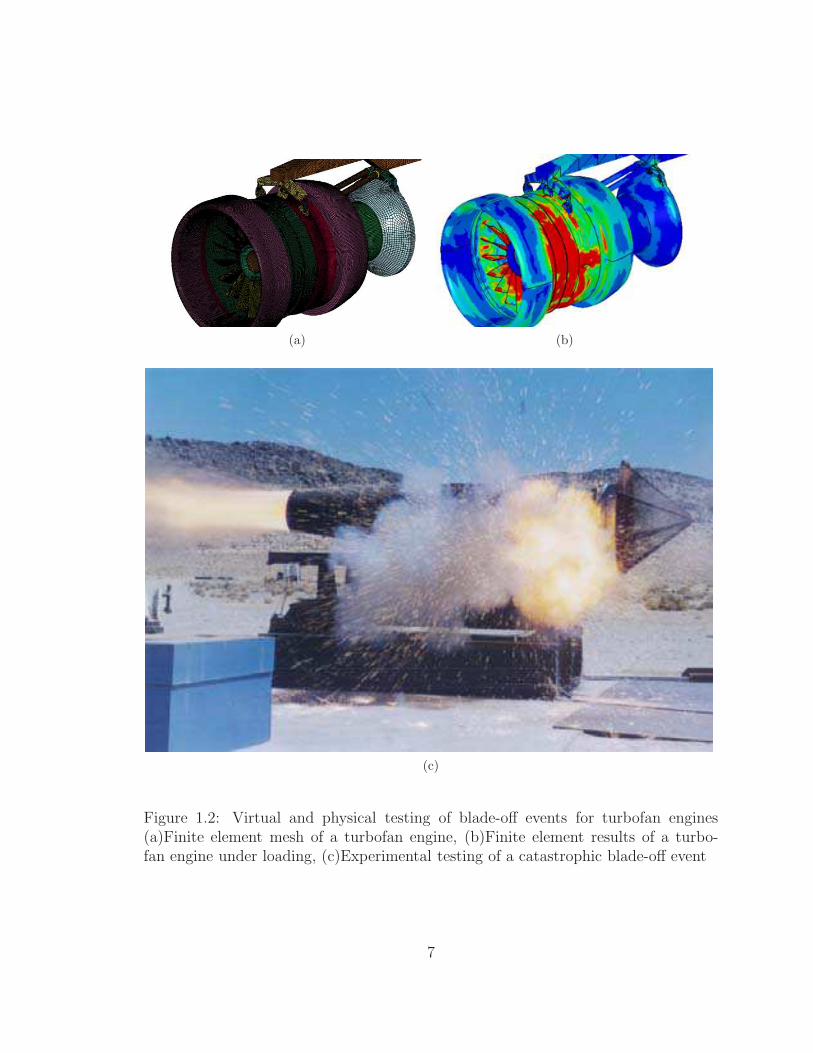
(a) (b)
(c)
Figure 1.2: Virtual and physical testing of blade-off events for turbofan engines(a)Finite element mesh of a turbofan engine, (b)Finite element results of a turbo-fan engine under loading, (c)Experimental testing of a catastrophic blade-off event
7

Although the plates are not all from the same sources they do have similar chemical
makeups and are compliant with the same Aerospace Materials Standards (AMS),
therefore the mechanical properties should be comparable. Great care is taken to
ensure the specimens are from the correct plate stock so results are not be corrupted.
Results from the individual plate stocks as well as a comparison between the four are
presented and discussed. These data are delivered to GWU for use in developing the
LS-DYNA material model MAT224 for Ti-6Al-4V which will be used in the FAA’s
ongoing Uncontained Engine Debris Mitigation Program.
Table 1.1: Material composition of the various plate stocks tested
Plate Plate Material Ingot Rolling Chemical Makeup (wt%)*No. Thick Source Source Source Al V Fe O C N Ti
1 2.29mm
Tri-Tech
RTIRMI
6.74 4.07 0.16 0.151 0.003 0.006 balTitanium
2 3.56mm TIMET TIMET 6.56 3.99 0.15 0.146 0.017 0.006 bal
3 6.35mm RTIAllegheny
6.13 3.97 0.18 0.173 0.016 0.006 balLudlum
4 12.7mmTitanium
TIMET TIMET 6.64 4.04 0.13 0.190 0.011 0.006 balInd.
*Chemistry presented from measured values completed at NASA - Glenn Research Center
This study characterizes the plate’s strain rate and temperature dependence as
well as its initial anisotropy with respect to plasticity. Stain rate dependence of the
material is found by testing in tension, compression, and shear (torsion) at strain
rates ranging from 1.0 × 10⁻⁴s−1 to 8.0 × 10³s−1. Temperature tests are conducted
for tension, compression, and shear at temperatures ranging from −50C to 600C.
8

Initial anisotropy in the plate is determined from tension and compression tests on
specimens fabricated in several orientations.
Ductile fracture of the 12.7mm plate is studied for the in order to generate a frac-
ture locus. This test series requires specimens with several different geometries which
introduces several stress states. Multiple stress states are used so that the locus plot
is sufficiently populated. Tension tests are conducted on specimens with geometries of
plane stress (thin, flat), axisymmetric, and plane strain (wide). Other states of stress
can be achieved through the testing of combined axial-torsional loading of thin walled
tube specimens. Experimental results coupled with LS-DYNA simulations allow the
state of stress at each fracture point to be recorded.
1.2 Literature Review
Some aspects of plastic deformation and the ductile fracture of Ti-6Al-4V have
been investigated by other researchers. Plastic deformation has been previously eval-
uated for strain rate and temperature dependence[12, 13, 14, 15, 16, 17]. Anisotropic
properties of the material have also been explored. Limited work has been performed
on the fracture characteristics of Ti-6Al-4V as well[5, 18, 19, 20].
The outline of this research is modeled after the work done by Seidt[21] on alu-
minum 2024-T351. The work presented here along with the work completed by Seidt
fall under the same body of work and have similar goals. Some aspects of the two
works will be comparable including specimen geometries, test setups, test methods,
and data analysis.
9

1.2.1 Plastic Deformation Behavior of Ti-6Al-4V
Many researchers have previously tested and analyzed Ti-6Al-4V for the plastic
deformation properties under different loading conditions. Yatnalkar[12], investigated
the strain rate dependence of Ti-6Al-4V under tension, compression, and torsion.
Significant strain rate dependence was reported for all loading conditions studied with
increases of 50, 56, and 77 percents for compression, tension, and torsion loading cases
respectively, for strain rates ranging from 1.0× 10⁻⁴s−1 to greater than 1300s−1. The
work by Yatnalkar[12] also includes anisotropic data for tension and compression,
finding flow stresses with variations of 13% and 14% respectively. Finally, Yatnalkar
presented elevated temperature data for compression which showed a decrease of
flow strength of 54% over a temperature range of 25C to 600C. As a continuation
of the program, this work continue tests with the same plate used by Yatnalkar to
reduce external variables that may contaiminate the data. Additional testing will
be performed to determine properties for compression loading at −50C as well as
tension ranging from −50C to 600C. A direct comparison from Yatnalkar’s raw data
will also be made here. Comparison of these plates is shown in Chapter 3.
Other researchers have determined the strain rate sensitivity of this material in-
cluding Wulf[13], Follansbee, et al.[14], Lee, et al.[15], Lee, et al.[16], Lee, et al.[17].
Results from the work by Follansbee, et al.[14] showed a high strain-rate sensitivity
of both the yield and flow stresses for several microstructures. The work by Wulf[13]
displayed increasing bilinear strain rate dependence for Ti-6Al-4V in compression
at strain rates of 3 × 10³s−1 to 3 × 10⁴s−1. Lee, et al.[15] presents Ti-6Al-4V data
at strain rates of 0.02s−1, 0.1s−1, and 1.0s−1 at temperatures ranging from 25C to
500C in compression. The researchers found that yield strength increases with strain
10

rate at similar temperatures but decreases with temperature at similar strain rates.
They also observed that work hardening decreases as the temperature and strain rates
increase. They attributed this to thermal softening which was present at the high
temperature and strain rate tests. The former is due to the nature of the test but
the latter develops the temperatures due to adiabatic heating during deformation.
Another work by Lee, et al.[16] investigates the effects of temperature at high strain
rates on Ti-6Al-4V with similar results. They also found that the work hardening
of the material decreases considerably as the testing temperature and strain rate in-
crease. Lee, et al.[17] also investigates the shear properties of Ti-6Al-4V at strain
rates of 1.8×10³s−1 to 2.8×10³s−1 and temperatures of −100C to 300C. This work
once again demonstrated the material has a significant temperature and strain rate
dependence.
Multiple researchers have found Ti-6Al-4V material parameters for the Johnson-
Cook constitutive model including Johnson et al.[22], Lesuer[22], Yatnalkar[12], and
Milani et al.[23]. The results from these studies are presented in Table 1.2. A com-
parison of these parameters are shown with data in Chapter 3.
Table 1.2: Johnson-Cook constitutive parameters for Ti-6Al-4VName A(MPa) B(MPa) C m n D1 D2 D3 D4 D5
Johnson 862 331 0.012 0.8 0.34 −0.09 0.25 −0.5 0.014 3.87
Lesuer 1098 1092 0.014 1.1 0.93 – – – – –
Yatnalkar 1055 426 0.023 0.8 0.50 – – – – –
Milani 1051 924 0.0025 0.98 0.52 – – – – –
11

Although some of these experimental properties have been previously determined,
this work is the first to include strain rate, temperature, and isotropic effects from a
single plate. It is also the first to compare similar tests between multiple plate stocks.
In this work, tension, compression, and shear tests are conducted on samples fabri-
cated from the same plate. Previous works[12, 13, 14, 15, 16, 17], typically conduct
only shear or tension tests, not all three. In addition to the plastic deformation test-
ing, the fracture test series is conducted on the same stock. Data from this project
is delivered to GWU for MAT224 development.
1.2.2 Ductile Fracture
Ductile fracture material characterization is valuable information for the analysis
of failure and is needed for proper material modeling. Impact events often give rise to
complex multiaxial stress states that include combinations of tension, compression,
and shear. Many researchers[5, 18, 19, 20], have discovered that the state of stress can
cause significant changes to the failure strain of a material undergoing complex loading
conditions. Theories attribute this to void nucleation, coalescence, and eventually
growth which then leads to complete failure. Rice and Tracey[18] showed that the
growth of a void could be represented macroscopically by the triaxial stress, σ∗,
and plastic strain. Bau and Wierzbicki[19] explored various specimen geometries
and concluded that ductile fracture was strongly based on stress triaxiality. Stress
triaxiality which is the ratio of mean stress, σm, to effective stress, σ, is defined as:
σ∗ =σm
σ, (1.4)
where,
σm =1
3σkk =
1
3(σ11 + σ22 + σ33) , (1.5)
12

σ =
(
3
2SijSij
)1
2
, (1.6)
where, Sij, is the deviatoric stress tensor or:
Sij = σij −1
3σkkδij . (1.7)
Barsoum and Faleskog[24] found that stress triaxiality of a specimen was insuf-
ficient to describe material fracture behavior, especially at low levels of triaxiality.
The researchers also investigated Lode parameter which was found to be an impor-
tant variable in the characterization of fracture and is given by
µ = −2σ1 − σ2 − σ3
σ1 − σ3
, (1.8)
where, σ1, σ2, and σ3, are the principle stresses and σ1 ≥ σ2 ≥ σ3. Xue [20] showed
a plasticity damage model that utilizes both stress triaxiality and Lode parameter to
describe the stress space of a specimen. The fracture model thus becomes a complex
function of both stress triaxiality and Lode parameter in the form of
ǫpf = f (σ∗, µ) . (1.9)
The goal of this portion of the work is to gain an understanding of the fracture char-
acteristics of Ti-6Al-4V and ultimately utilize these parameters to create a fracture
locus. The locus will be applied to plastic deformation results to form a material
model used in the finite element calculations. To accurately represent the entire
stress-space, multiple data points and thus multiple tests are required.
Johnson[22] determined the fracture model constants for Equation 1.2 seen in
Table1.2. This model, however only takes into account stress triaxiality. In this
work, both triaxiality and lode parameter are used to describe the material’s fracture
13

behavior. In addition, Johnson-Cook fracture model parameters are determined for
tests conducted in this work. Johnson’s model and the new parameters are compared
in Chapter 4.
Although similar tests have been previously preformed this work represents the
most comprehensive database of plastic deformation and fracture data for Ti-6Al-4V.
Ultimately, these data will be delivered to researchers at GWU and used to refine the
MAT224 failure model.
14

Chapter 2: Experimental Procedures and Techniques
2.1 Introduction
This chapter presents experimental programs for plastic deformation and duc-
tile fracture test series as well as the experimental techniques that are employed to
conduct them. These test plans are presented with explanation for each of the tests.
The quasi-static and dynamic testing methods and calculations are presented and dis-
cussed. Limited tests are performed on the 2.29mm and 3.56mm sheet stocks (plate
1 and 2 respectively) to show overall trends in the material characteristics. Strain
rate characterization, anisotropic testing, and limited temperature testing has been
preformed previously on the 6.35mm plate (plate 3)[12]. On this same plate tests are
completed in tension at high and low temperatures as well as in compression at low
temperatures. Finally, a 12.7mm plate (plate 4) is studied in depth under similar
conditions as plate 3 in addition to shear. Plate 4 is also tested to understand the
fracture characteristics of the material.
A break through in strain measurement called Digital Image Correlation (DIC)
which is described in detail by Sutton, Orteu, and Schreier[25] is an optical method
to measure full field strains of a deforming specimen. This method of measurement
15

provides good spatial resolution on the surface of a deforming specimen. This mea-
surement technique is briefly discussed in this chapter.
This section also presents the mechanical methods used to test the material spec-
imens. Several machines are used to conduct the tests outlined in this chapter. The
DMML always strives to provide high quality data and therefore has developed orig-
inal testing procedures. A new method, using DIC, is implemented in conjunction
with this project. A method, first proposed and used in this work, to measure full
field strains with DIC at elevated temperatures is discussed in detail in Chapter 6.
2.2 Plastic Deformation of Ti-6Al-4V
Plastic deformation of Ti-6Al-4V is investigated in the specific program presented
in Table 2.1. Testing is preformed at several strain rates to gain an understanding
of the strain rate dependence of the material. Anisotropic properties of the material
are examined at several loading orientations. Lastly, the temperature dependence is
investigated at several temperatures within the material’s operational range.
For plate stock 1 and 2, strain rate dependence is determined in tension at strain
rates of 1.0s−1 and 5.0×10²s−1 and at rates of 1.0s−1 and 1.5×10³s−1 for compression.
In addition to the rolled direction, tension tests are conducted at different orientations
(90 and 45) to determine its degree of anisotropy at a strain rate of 1.0s−1. Due to
size limitations, compression specimens are only fabricated from the through direction
and therefore anisotropic tests cannot be conducted. Specimens are orientated in the
directions illustrated in Figure 2.1. Results from these tests are presented in Chapter
3.
16

Table 2.1: Experimental outline for the plastic deformation testing of Ti-6Al-4VTest Loading Testing Strain Rate Specimen Temp PlateNo. Mode Apparatus (1/s) Orientation ( C) Stock
1
Tension
Hydraulic 1.00E-4
Rolled
Room Temp
3*,42 Load 1.00E-23 Frame 1.00E0
1,2,3*,44 Kolsky 5.00E25 bar 1.50E3 3*,46
1.00E0
45From Rolled1,2,3*,4
7 Transverse8 Hydraulic -45From Rolled 3*,49 Load
Rolled
200
3,410 Frame 40011 60012 -5013
Compression
Hydraulic 1.00E-4Rolled
Room Temp
3**,414 Load 1.00E-215 Frame 1.00E0 3*,415 1.00E0 Through 1,216
Kolsky Bar1.50E3
Rolled 3**,417 3.00E316 1.50E3 Through 1,218
1.00E0
45From Rolled
3*,4
19 Transverse20 -45From Rolled21 Hydraulic Through22 Load
Rolled
20023 Frame 40024 60025 -5026
Torsion
Hydraulic 1.00E-4
Through
Room Temp
4
27 Load 1.00E-228 Frame 1.00E029 Kolsky 5.00E230 bar 1.50E331
1.00E0
20032 Hydraulic 40033 Load 60034 Frame -50
*Tests Completed by Ravi Yatnalkar[12]**Tests Completed by Both Researchers
17

Figure 2.1: Specimen manufacturing orientation for the 2.29mm, 3.56mm, and6.35mm plate stocks
The 6.35mm plate, labeled plate 3, was extensively tested and presented by
Yatnalkar[12] under the same project. This plate was tested in tension at strain
rates of 1.0 × 10⁻⁴s−1 , 1.0 × 10⁻²s−1, 1.0s−1, 5.0 × 10²s−1, and 1.5 × 10³s−1. The
plate was also tested in a range of orientations to check for anisotropic effects in the
material at a strain rate of 1.0s−1. In this work, tension testing at temperatures
of −50C, 200C, 400C, and 600C are completed. Compression tests were previ-
ously completed at strain rates of 1.0× 10⁻⁴s−1 , 1.0× 10⁻²s−1, 1.0s−1, 1.5× 10³s−1,
and 3.0 × 10³s−1, elevated temperatures ranging from 200C to 600C, and on spec-
imens with various orientations. Compression tests are conducted here at −50C to
complete the temperature test series for plate 3. Specimens for plate 3 were also
fabricated in the directions shown in Figure 2.1. Results from these additional tests
and a comparison to the other tests are presented in Chapter 3.
18

Figure 2.2: Specimen manufacturing orientations for the 12.7mm plate stock
The 12.7mm plate, labeled plate 4, is tested in tension and shear at strain rates
of 1.0 × 10⁻⁴s−1, 1.0 × 10⁻²s−1, 1.0s−1, 5.0× 10²s−1, and 1.5× 10³s−1. Compression
tests are completed at strain rates of 1.0×10⁻⁴s−1, 1.0×10⁻²s−1, 1.0s−1, 1.5×10³s−1,
3.0× 10³s−1, and 8.0× 10³s−1. Tension anisotropic effects in tension are investigated
in the rolled, 45 from rolled, transverse, and −45 from rolled directions at a strain
rate of 1.0s−1. Compression anisotropy effects are determined from tests at these
orientations in addition to the through direction. Tests are conducted in tension,
compression, and shear at temperatures ranging from −50C to 600C at a strain
rate of 1.0s−1. Temperature specimens are made from the rolled direction for tension
and compression and in the through direction for the torsion specimens. Fabrication
directions are shown in Figure 2.2. This plate stock is also used to determine of the
fracture characteristics of the material.
19

2.2.1 Tension Experiments
Plastic deformation tension tests are conducted on thin flat dog-bone specimens.
The specimens have size constraints due to the nature of the high strain rate testing.
The strain rate of a specimen in a Kolsky bar, which will be discussed later, is
inversely proportional to the gage length. For consistency, specimen geometry for all
strain rate, temperature, and orientation tests are conducted on the same specimen
geometry, seen in Figure 2.3
Figure 2.3: Plane stress smooth specimen used in plastic deformation testing
The tension specimens have their profiles cut out and are sliced from the plate
stock with the use of Electrical Discharge Machining (EDM). To ensure the base
material is tested the specimens are precision ground to remove the EDM recast
layer. Since the side of the gage section comparatively represents a much smaller area
in comparison this is assumed to have a limited affect on the data and therefore not
ground. Due to small variabilities in the specimen gage cross-section sizes, dimensions
are measured and recorded prior to testing.
Force, F , and displacement, ∆L, are recorded for all tension tests. Engineering
stress, σe, and engineering strain, ǫe, are calculated for these records. These are given
20

by,
σe = F/A, (2.1)
and
ǫe = ∆L/lg, (2.2)
where, A is the cross sectional area of the specimen, and lg is the initial specimen
gage length.
2.2.2 Compression Experiments
Compression tests are conducted on a solid cylindrical specimen, as seen in Figure
2.4. The length to diameter ratio of the compression specimens is kept close to one
to limit buckling during testing. If buckling occurs, a complex stress state exists and
the test is no longer uniaxial.
Figure 2.4: Compression specimen used in plastic deformation testing
Specimens are cut from the plate using conventional machining and turned to size
on a lathe. In order to maintain uniaxial stress, the parallelism of the top and bottom
of the specimen is controlled to within 0.025mm. Specimen dimensions are carefully
measured and recorded prior to testing to monitor slight differences in fabrication.
21

Force and displacement are also recorded for the compression testing where the stress
and strain will be negative. This negative value is consistent with compressive load
and negative change in length.
2.2.3 Shear Experiments
Shear properties for Ti-6Al-4V are determined using of thin-walled torsion speci-
mens shown in Figure 2.5. The specimens seen here are the high strain rate specimens
which are glued into an adapter. The low strain rate specimens have a hexagonal grip-
ing section so the screws, which are also placed in a hexagonal arrangement, align
with the specimen. For strain rates of 1.0 × 10⁻⁴s−1 to 5.0× 10²s−1 the gage length
is 2.54mm. For the highest strain rates (> 1.5 × 10²s−1) the gage length is reduced
to 1.78mm since the strain rate is inversely proportional to gage length. The inside
diameter and wall thickness dimensions are identical.
Figure 2.5: Torsion specimen used in plastic deformation testing
Shear stress, τ , and shear strain, γ, and are given by
22

τ =T
2πr2mh, (2.3)
and
γ =θrmLs
, (2.4)
where, T is the measured torque, rm is the mean radius, J is the polar moment of
inertia, θ is the angle of rotation, and Ls is the gage length of the specimen. A
geometric representation of the shear specimen gage section is shown in Figure 2.6.
Figure 2.6: Geometric representation of the shear stress calculation
Shear displacements are calculated by tracking the relative motion of two points
in space at the top and bottom of the specimen. As the points move during the test,
the x and z displacements for both the top and bottom points are tabulated, shown
in Figure 2.6. The angle of twist, ∆θ, is calculated by taking the difference of the top
23

and bottom points. The angle is calculated by
∆θ = arccos
(ro −∆z)2 + r2o −∆x2
2 [ro − (ro −∆z)]
, (2.5)
where, ro, is the outside radius, ∆z, is the z displacement, ∆x, is the x displacement.
2.2.4 Comparison of the Results from the Plastic Deforma-
tion Testing
Tension and compression engineering stress-strain curves look very different as
seen in Figure 2.7. These curves do not match in part because of transverse deforma-
tion. In tension, the cross-section of the sample reduces as it extends. In compression
the cross-section of the sample increases as it is compressed. Engineering stress is
simply the load divided by initial area. True, or logarithmic stress strain takes into
account this positive or negative change in cross sectional, making it a better metric
to compare the two modes of loading. These values are given by
ǫt = ln (1 + ǫe) , (2.6)
and
σt = σe (1 + ǫe) , (2.7)
where, ǫt is true strain, ǫe is engineering strain, σt is true stress, and σe engineer-
ing strain. Once localization occurs these formulae are no longer valid because the
deformation is no longer uniform.
Shear tests are compared here by calculating the effective stress and equivalent
strain. Effective stress, σeff , is found by substituting a pure shear stress state into
Equation 1.6. The result is,
σeff =√3τ, (2.8)
24

0 0.05 0.1 0.15 0.2 0.25 0.30
200
400
600
800
1000
1200
1400
1600
1800
2000
Strain
Str
ess
(MP
a)
Tension (Engineering)Tension (True)Compression (Engineering)Compression (True)Torsion (Shear)Torsion (Effective)
Figure 2.7: Comparison of stress strain calculation types for the different loadingconditions
Similarly the equivalent strain increment, dǫeff is given as
dǫeff =
(
1
2dǫijdǫij
)1
2
=dγ√3, (2.9)
where,
ǫij =
0 γ/2 0γ/2 0 00 0 0
. (2.10)
These values can then be easily compared to the tension and compression effective
stress-strain curves shown in Figure 2.7. Here we can see the elastic modulus in shear
is now in agreement with the moduli for tension and compression. The stress levels
in tension, compression, and shear do not match. This, however, is a property of
Ti-6Al-4V plate and is exhibited in some other materials.
2.3 Ductile Fracture of Ti-6Al-4V
Ductile fracture testing is conducted on several different specimen types including
plane stress (thin, flat specimens), plane strain (thick, flat specimens), axisymmetric
25

(round), and combined loading (thin walled tube). These specimens are all fabricated
from plate 4. All specimens are fabricated with the loading direction parallel to the
rolled direction shown in Figure 2.8.
Figure 2.8: Fracture specimen manufacturing orientations for the 12.7mm plate stock
All tests are conducted with a cross head velocity of 0.254mm/s which represents a
strain rate close to 1.0×10⁻²s−1. Due to strain localization caused by different stress
states the strain rate of the tension experiments will vary between tests. Combined
loading tests undergo an increasing strain rate since the stress state is maintained in
load and torque control.
The various stress states explored in this test series are used to construct a frac-
ture locus. Several different geometries of the specimen types are used in order to
effectively populate the locus used in the fracture model for MAT224. These various
26

specimens provide a range of values for both the triaxiality and Lode parameter. As
seen in Figure 2.17, both the stress triaxiality and Lode parameter change through-
out the test. In order to quantify the stress state, ultimately to create the fracture
surface, representative values must be given to the stress state of the specimen. The
stress state parameters presented here are weighted with the specimen plastic strain.
The average stress triaxiality is given by
σ∗ =
∫
σ∗dǫp
ǫpf(2.11)
With the average Lode parameter is given by
µ =
∫
µdǫp
ǫpf(2.12)
Numerical simulations, which are completed with LS-DYNA, are used to design
the specimens used in the fracture test series. Plane stress samples are designed such
that the stress triaxiality ranges from 0.400 for a smooth gage section to 0.583 with
a sharp notch. Plane strain samples have a thick gage section to achieve a state of
plane strain in the center of the specimen. A thickness of 25.4mm was determined
to yield plane strain conditions by other researchers[21]. Stress triaxialities of 0.470
and higher can be achieved with a smooth gage section and notches of varying radii.
Axisymmetric samples are capable of obtaining stress triaxialities ranging from 0.369
for a smooth gage section to nearly hydrostatic tension (σ1 >> σ2 = σ3 or σ∗ = 1)
for a sharp notch radius. Since the axisymmetric samples have the ability to bridge
stress triaxiality values of both the plane stress and plane strain specimens, they will
be used to compare similar stress states.
Simulations are run in LS-DYNA to design specimens with specific average stress
triaxialities and Lode parameters. For all simulations, meshes are constructed such
27

that the element lengths are constant at 0.152mm/element. The resulting mesh den-
sity translates to 5 elements across the thickness of the plane stress samples, 32
elements across the minimum notch diameter of the axisymmetric samples, and 167
elements across the thickness of the plane strain samples. Hypermesh version 9.0
is used to create the meshes, which can be seen in Figure 2.9. The Johnson-Cook
material model (MAT015) is used for these initial tests. The parameters used were
those found by Lesure[22] and are tabulated in Table 1.2. Complete meshes for each
of the specimens is presented in Appendix C
Figure 2.9: Points of interest for: (a)plane stress, (b)axisymmetric and (c)plane strainspecimens
The failure point of interest for each of the specimen types is taken from the
center most point, as shown in Figure 2.9. This point of interest is used because
28

the void nucleation is assumed to begin here. Element aspect ratios near this point
are nearly 1.0. For axisymmetric meshes the element aspect ratio increases moving
radially outward from the center of the cross-section. This was deemed acceptable
since stress state of interest lies on the axis of symmetry where the aspect ratio is
nearly 1.0. Load is applied to the specimen by fixing one end and applying a constant-
velocity actuator motion to the other.
2.3.1 Plane Stress Fracture Testing
Thin flat specimens are tested to approximate a state of stress where the out of
plane stress is zero giving rise to the plane stress condition. This state is shown
in Figure 2.10. Plane stress testing includes specimens with several notch radii,
providing alternate stress states as seen in Table 2.2. Plane stress specimen geometries
are pre-determined based on the specimens used by Seidt[21]. The thickness and
notch width dimensions are set at 0.76mm and 3.05mm, respectively for the notched
specimens. The three notched specimens have radii of 14.29mm (SG2), 4.76mm
(SG3), and 0.40mm (SG4). Stress triaxialities and effective plastic fracture strains
are calculated from LS-DYNA simulations using the methods established above. The
results of these simulations are presented in Table 2.2. These simulations predict
average triaxialities ranging from 0.400 to 0.583 and Lode parameters ranging from
-0.014 to 0.845.
These specimens are manufactured using the same methods described for the
plastic deformation tension specimens (see section 2.2.1). All specimens are measured
prior to testing. Thickness and width at the minimum cross section are recorded.
29
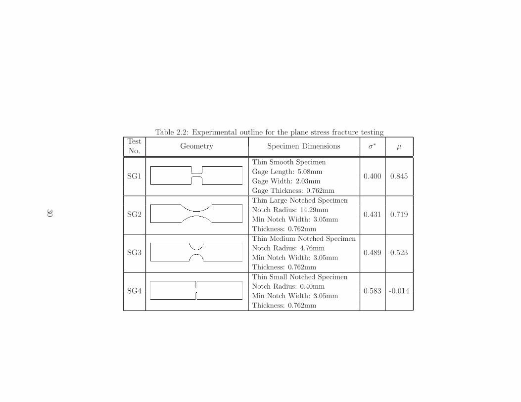
Table 2.2: Experimental outline for the plane stress fracture testingTest
Geometry Specimen Dimensions σ∗ µNo.
SG1
Thin Smooth Specimen
0.400 0.845Gage Length: 5.08mm
Gage Width: 2.03mm
Gage Thickness: 0.762mm
SG2
Thin Large Notched Specimen
0.431 0.719Notch Radius: 14.29mm
Min Notch Width: 3.05mm
Thickness: 0.762mm
SG3
Thin Medium Notched Specimen
0.489 0.523Notch Radius: 4.76mm
Min Notch Width: 3.05mm
Thickness: 0.762mm
SG4
Thin Small Notched Specimen
0.583 -0.014Notch Radius: 0.40mm
Min Notch Width: 3.05mm
Thickness: 0.762mm
30

Figure 2.10: State of stress in the plane stress tension specimen
2.3.2 Plane Strain Fracture Testing
Thick tension specimens are tested for a state of plane strain in the center of
the specimen, where ǫx, γxz, γyz are assumed to equal zero. Although the transverse
strains (ǫxx) near the edge are non-zero they become close to zero at the center of the
specimen. A graphical representation of this strain state can be seen in Figure 2.11.
Figure 2.11: State of strain at the center of the plane strain fracture specimen
31

Plane strain specimen geometries are pre-determined based on previous research
done by Seidt[21]. Three geometries are tested including a smooth gage section
and two notched specimens. The thickness and notch width dimensions were set at
25.4mm and 2.032mm, respectively along with two notch radii of 12.7mm, 4.763mm.
Simulations are run and stress triaxialities and Lode parameters are calculated. Re-
sults of these simulations are presented in Table 2.3. These specimens have average
triaxialities ranging from 0.470 to 0.768 and Lode Parameters ranging from 0.025 to
0.506.
32

Table 2.3: Experimental outline for the plane strain fracture testingTest
Geometry Specimen Dimensions σ∗ µNo.
SG11
Axisymmetric Smooth Specimen
0.470 0.506Gage Length: 10.16mm
Gage Width: 2.03mm
Gage Thickness: 25.40mm
SG12
Axisymmetric Notched Specimen
0.660 0.040Notch Radius: 12.70mm
Gage Width: 2.03mm
Gage Thickness: 25.40mm
SG13
Axisymmetric Notched Specimen
0.768 0.025Notch Radius: 4.76mm
Gage Width: 2.03mm
Gage Thickness: 25.40mm
33

2.3.3 Axisymmetric Fracture Testing
Axisymmetric specimens have a circular cross sectional area in the gage section.
This geometric shape creates a state of stress where σy ≫ σx = σz. The stress state
can be seen in Figure 2.12. Since σ2 = σ3 or σx = σz , the Lode parameter (Equation
1.8) for all axisymmetric specimens is 1.0. These specimens have the ability to cover
triaxiality ranges of both the plane strain and plane stress specimens.
Figure 2.12: State of stress in the axisymmetric fracture specimen
Five axisymmetric geometries are determined such that the resulting average stress
triaxialities are close to those from the plane stress and plane strain specimens. The
minimum gage diameter for each axisymmetric specimen is set at 4.763mm. The
notch radii are determined iteratively with the initial trial radius determined from
Bridgemans analytical solution of the stress field at the neck of an axisymmetric tensile
bar[26]. The following equation[26] relates the stress triaxiality to the dimensions of
the necked sample given by
σ∗ =1
3+ ln
(
1 +a
2R
)
, (2.13)
34

where, a is the minimum cross-sectional radius, and R is the radius of the notch or
neck. A sketch showing the critical dimensions of this analysis is shown in Figure
2.13[27].
Figure 2.13: Sketch of Bridgman’s analysis of a necked axisymmetric sample
Using the methods established in the previous section, a simulation of the trial
geometry is performed and the stress triaxiality and effective plastic fracture strain
are calculated. It should be noted that as the specimen deforms the stress state is
evolving which makes the Bridgman’s approximation unreliable.
An iterative process is used to determine the notch radius required to approxi-
mately match the stress triaxiality of either a plane stress or plane strain specimen. If
the axisymmetric average value is within 5% of the target value, it is determined that
the radius is acceptable and the iterative process is complete. If the axisymmetric
triaxiality is outside of the acceptable range (error ≥ 5%), a new radius is determined,
the mesh is constructed and the simulation run. Since the notch radius is inversely
proportional to the stress triaxiality, an approximation for next trial radius is made.
35

The final specimen dimensions are listed along with the resulting average triaxialities
and Lode parameters in Table 2.4.
Attempting to match the plane stress SG4 sample leads to an unreasonably large
notch radius. Due to this, there is no match to this plane stress specimen but a smaller
notched axisymmetric specimen (SG10) is added to extend the covered triaxiality
range. The results of this iterative procedure led to simulated average triaxialities
ranging from 0.369 to 0.956 and Lode parameters of 1.0.
These specimens were fabricated by first taking a cylindrical slug oriented with
its axis parallel to the rolled direction with an EDM machine. Second, the notches
are turned down using a CNC lathe to maintain a consistent radius.
36
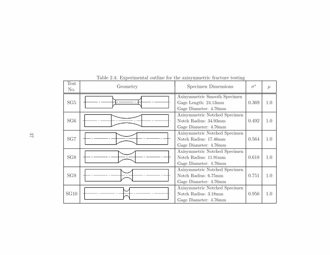
Table 2.4: Experimental outline for the axisymmetric fracture testingTest
Geometry Specimen Dimensions σ∗ µNo.
SG5Axisymmetric Smooth Specimen
0.369 1.0Gage Length: 24.13mm
Gage Diameter: 4.76mm
SG6Axisymmetric Notched Specimen
0.492 1.0Notch Radius: 34.93mm
Gage Diameter: 4.76mm
SG7Axisymmetric Notched Specimen
0.564 1.0Notch Radius: 17.46mm
Gage Diameter: 4.76mm
SG8Axisymmetric Notched Specimen
0.618 1.0Notch Radius: 11.91mm
Gage Diameter: 4.76mm
SG9Axisymmetric Notched Specimen
0.751 1.0Notch Radius: 6.75mm
Gage Diameter: 4.76mm
SG10Axisymmetric Notched Specimen
0.956 1.0Notch Radius: 3.18mm
Gage Diameter: 4.76mm
37

2.3.4 Combined Loading Testing
An effective method of populating additional points on the fracture locus is to use
combined loading experiments[21] where a tubular specimen under goes a torsion-
tension, torsion-compression, or pure torsion loading as seen in Figure 2.14. A wide
range of stress states can be achieved by varying the ratio between the specimen’s
axial stress and shear stress. The axial load, P , can be positive or negative, giving
tensile or compression stress, respectively. The specimen is also subjected a torque,
T , creating a state of stress unlike those presented previously. This state has both
σx and τxy as seen in figure 2.14, the magnitudes of which can be manipulated giving
various stress states. The stress state is
σ =
σx τxy 0τxy 0 00 0 0
. (2.14)
The stress triaxiality is
σ∗ =σm
σ=
σx
3(
σ2x + 3τ 2xy
)1
2
=σx/τxy
3√
3 + (σx/τxy)2, (2.15)
and the Lode parameter (equation 1.8) is
µ =σx
2√
(
σx
2
)2+ τ 2xy
=
√
σx/τxy4 + σx/τxy
. (2.16)
Using Equation 2.15 and 2.16 the triaxiality and Lode parameter can be found
from stress ratios. The curves in Figure 2.15, determine the ratio of axial stress to
torsional stress needed to provide the desired state of stress. It should be noted that
this state of stress is relatively simple and does not evolve during the test. Therefore,
parallel finite element analysis is not required to determine specimen geometries. The
geometries for the combined loading tests (summarized in Table 2.5) are taken from
Seidt[21] to maintain consistency in testing techniques under the same project.
38

Figure 2.14: State of stress within a combined loading specimen
These tests are largely dependent on the axial torsional stress ratio, where σx/τxy >
0 signifies a tensile axial load and σx/τxy < 0 is compressive. Pure shear is obtained
from σx/τxy = 0. The combined loading stress state parameters are mathematically
limited to a range of triaxialities and Lode numbers. Stress triaxialities can range
from -0.333 to 0.333 while Lode parameter can range from -1.0 to 1.0. Loading ratios
(σx/τxy) of 1.971, 0.847, 0.00, and -0.847 were chosen for these experiments, which
correspond with experiments done previously[21]. Torsion-compression tests are prac-
tically limited due to the potential for buckling in the specimen, which would result
in an unwanted complex stress state.
The plane stress, plane strain, and axisymmetric specimens were fabricated from
plate 4 all with the loading direction parallel to the rolled direction as seen in Figure
39

Table 2.5: Experimental outline for the combined loading fracture testingTest
Geometry Specimen Dimensions σ∗ µσy
τxyNo.
LR1
Combined Tension-Torsion
0.251 0.702 1.971Gage Length: 3.18mm
Inside Diameter: 7.93mm
Outside Diameter: 9.14mm
LR2
Combined Tension-Torsion
0.147 0.390 0.847Gage Length: 3.18mm
Inside Diameter: 7.93mm
Outside Diameter: 9.14mm
LR3
Pure Shear
0.000 0.000 0.00Gage Length: 3.18mm
Inside Diameter: 7.93mm
Outside Diameter: 9.14mm
LR4
Combined Compression-Torsion
-0.147 -0.390 -0.847Gage Length: 3.18mm
Inside Diameter: 6.35mm
Outside Diameter: 9.14mm
40

−4 −3 −2 −1 0 1 2 3 4−1
−0.8
−0.6
−0.4
−0.2
0
0.2
0.4
0.6
0.8
1
Torsion−Compression→
Pure Shear→
←Torsion−Tension #1
←Torsion−Tension #2
Ratio of Stress Components (σx/τ
xy)
Par
amet
er V
alue
(σ*,
µ)
Stress TriaxialityLode Parameter
Figure 2.15: Stress state parameters for the combined loading specimens at differingstress component ratios
2.8. The line of symmetry for the torsion spool specimens, used in the plastic defor-
mation tests, lies along the through direction of the plate. Due to the differences in
fabrication orientation, varying results may be seen between the two sets of data.
2.3.5 Fracture Parameter Determination
Parallel simulations are completed for each tension fracture specimen to find the
state of stress and equivalent plastic fracture strain, as seen in Figure 2.16. Theory
predicts that the failure will occur due to the coalescence of voids at the center of the
specimen[28]. Therefore stress state and plastic strain must also come from this point
(see point of interest in Figure 2.9). Digital Image Correlation can only measure the
surface strains of a specimen, however, the point of interest is in the interior of the
specimen. LS-DYNA simulations are completed with the same mesh parameters as
41

those used for the initial specimen design process. Meshes for each of the specimen
types can be seen in Appendix C. A Simplified Johnson-Cook (MAT098) material
model calibrated with the data from the plasticity test series is used to model the
specimen material. The mesh is constructed for three dimensional constant stress
elements. The simulations are intentionally run without a failure model. Simulated
results are manually truncated to match the force displacement curve of each exper-
iment. The truncation of simulated data occurs where the experimental specimen is
unloaded due to failure. Results are presented in Chapter 4
The principle stresses, effective stress, effective plastic strain, and directional
strains are extracted and tabulated for each of the experiments. Simulated strains
from the surface of the specimen are compared to those measured experimentally.
The simulated reaction force of the constrained specimen is also compared to exper-
imental load data. Stress triaxiality and Lode parameter are determined from the
data recorded at the point of interest using equations 1.4 and 1.8 respectively.
Experimental (DIC) and simulated displacement data are synchronized, as seen
in Figure 2.17. This plot shows the simulated and experimental stresses in blue, the
strains in green, and the stress state parameters in red. The simulated interior strains
differ from the simulated surface strains. This is due to the difference in stress state
between the interior element and surface element. The surface strains measured with
DIC also disagree with the surface strains in the simulation. This is due to the fact
that the element size in the simulation is significantly smaller than the virtual strain
gage lengths of the DIC measurements. The simulated data is truncated at the point
that the physical specimen breaks. This break is signified by a rapid drop in load
which is shown as a gray vertical line. This is completed for each of the physical
42

tests and the corresponding stress state values are averaged, using Equation 2.11 and
Equation 2.12.
Figure 2.16: Strain comparison from an experimental axisymmetric notched specimenand parallel simulation
The combined loading specimen stress state is only dependent on the loading ratio,
which is directly proportional to the load and torque. Therefore no simulations are
needed. The fracture strain in this case is taken from DIC data. The virtual strain
gage length for these tests are similar to those used in the tension fracture tests.
Fracture strain and stress state data are used to create the fracture locus. These
data are presented and discussed in Chapter 4. A complete presentation of the data
for each of the specimens is found in Appendix D.
43

Figure 2.17: Example of history from an experimental plane stress smooth specimenand a parallel simulation
2.4 Quasi-static Strain Rate Testing Techniques
An Instron 1321 Servo-hydraulic biaxial load frame, see figure 2.18, is used to
conduct the fracture, anisotropic, temperature, and any strain rate test series (strain
rates at and below 1.0s−1). This machine has the capability to move axially ±61.2mm
and rotate±45. This one test apparatus can conduct uniaxial tension tests, compres-
sion tests, torsion tests, or a combination of these loading conditions. Measurements
are taken with two load cells: a Lebow 6467-107 with a capacity of 89kN (1100Nm)
and an Interface 1216CEW-2k with a capacity of 8.9kN (110Nm) depending on the
amount of force expected . This machine is controlled by an external computer and
an MTS FlexTest SE controller. The controller acquires data through MTS 493.25
Digital Universal Conditioners, with a maximum rate of data capture of 100kHz. The
44

load frame’s actuator is controlled from a Linear Variable Differential Transformer
(LVDT) and a Rotational Variable Differential Transformer (RVDT). Records from
these devices are also acquired however strain computations from these measurements
are susceptible to machine and grip compliance and can result in error.
Figure 2.18: Instron 1321 servo-hydraulic biaxial load frame equipped with hydraulicwedge grips
45

The DMML has multiple specimen griping options. Room temperature tension
tests with an axial load below 31kN are performed with MTS647.02B-22 hydraulic
wedge grips. These grips accommodate several different wedge designs. The flat
plane stress specimens are gripped with a flat knurled grip, while the axisymmetric
and combined loading specimens are gripped with a vee notch wedge. The plane strain
and combined loading specimens with an axial force greater than 31kN required the
MTS647.10A-11 hydraulic wedge grips which has a maximum axial load of 120kN.
For the high and low temperature testing, specially designed bars, long enough to
attach the specimens within the furnace, are used. The bars are fabricated from
Inconel 718 because of the material’s high strength, high operational temperatures,
and good thermal properties. The bars are equipped with cooling collars and various
heads depending on the loading type. The bars must be properly aligned since small
deviations of concentricity of the bars are detrimental to loading conditions and the
experimental results. Alignment is completed using two dial indicators set 90 apart
attached to the top or bottom collet fixture. As the actuator base is rotated ±90,
the indicators deviate either positive or negative thus showing the required direction
of bar adjustment. Bars are adjusted at the collet and aligned to within ±0.05mm
at the specimen attachment point. This process is completed for both the top and
bottom bars. Tension grips, also fabricated from an Inconel 718, thread into the 718
bars. These grips clamp the specimen into place using four #4-40 screws. Alignment
grooves in the tension grips are used to center the specimen during attachment.
Compression tests are conducted using steel push rods or Inconel bars as discussed
above. In all cases, Tungsten Carbide (WC) inserts are used as compression platens
to avoid fixture deformation. High and low temperature tests employ the previously
46
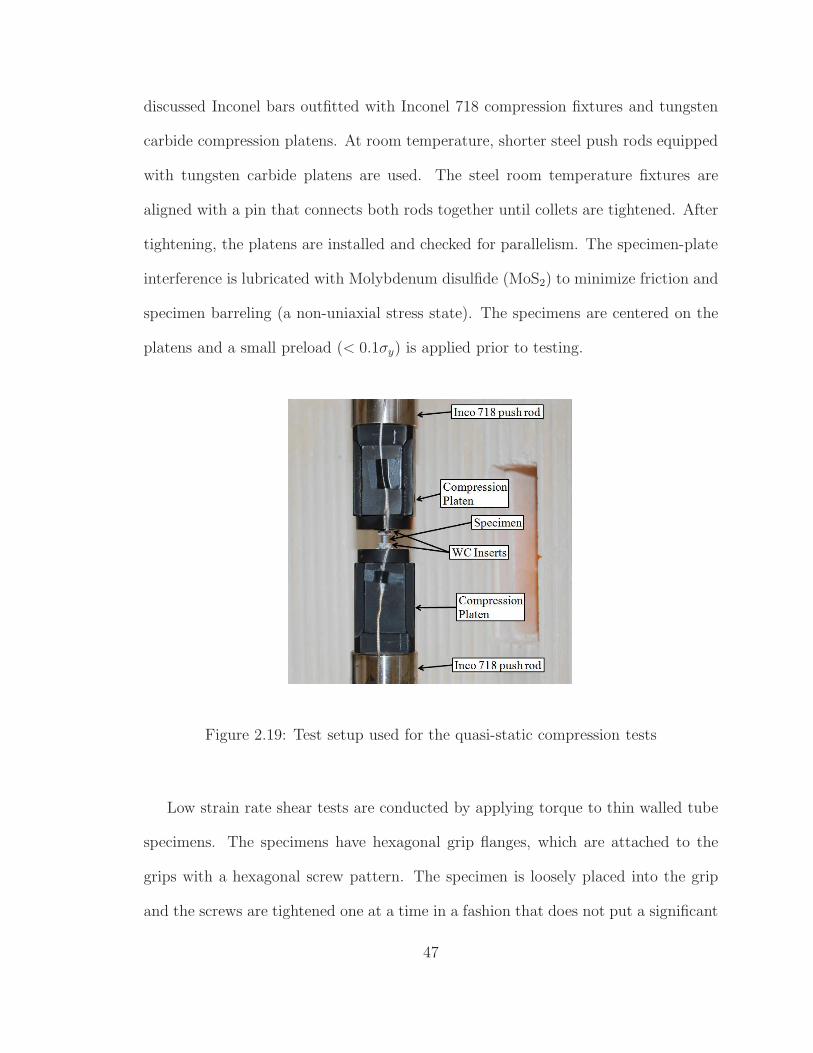
discussed Inconel bars outfitted with Inconel 718 compression fixtures and tungsten
carbide compression platens. At room temperature, shorter steel push rods equipped
with tungsten carbide platens are used. The steel room temperature fixtures are
aligned with a pin that connects both rods together until collets are tightened. After
tightening, the platens are installed and checked for parallelism. The specimen-plate
interference is lubricated with Molybdenum disulfide (MoS2) to minimize friction and
specimen barreling (a non-uniaxial stress state). The specimens are centered on the
platens and a small preload (< 0.1σy) is applied prior to testing.
Figure 2.19: Test setup used for the quasi-static compression tests
Low strain rate shear tests are conducted by applying torque to thin walled tube
specimens. The specimens have hexagonal grip flanges, which are attached to the
grips with a hexagonal screw pattern. The specimen is loosely placed into the grip
and the screws are tightened one at a time in a fashion that does not put a significant
47

amount of torque or axial load on the specimen. To ensure that the specimen is loaded
along the axis of the load frame, the outer diameter of the hexagonal specimen flange
is machined to match the inner diameter of the gripping bars. The grips are aligned
using the indicator method described previously. The bars are made from MAR-246,
a high temperature alloy. This method is used for the low, room and high temperature
testing.
2.5 High Strain Rate Testing Techniques
Dynamic behavior of Ti-6Al-4V is experimentally determined using the Kolsky
Bar or Split-Hopkinson Bar tests. This method, first proposed by Kolsky [29], uses
elastic stress wave propagation in two long bars to determine the dynamic plastic
deformation behavior of a specimen placed in the middle. This technique has become
a widely used method for dynamic testing and has been modified for both tension
and torsion. Typical strain rates of 500s−1 to 8000s−1 are obtained, depending on
the sample dimensions, strength, and the machine loading conditions. The following
section describes the Kolsky bars used by the DMML and appropriate data processing
techniques.
2.5.1 High Strain Rate Compression Testing
The compression Kolsky Bar at the DMML, see Figure 2.20 and 2.21, consists of
three 12.7mm diameter Ti-6Al-4V rods. The 610mm long striker bar is fired into the
incident bar at velocities up to 40m/s. The impact creates an incident wave that has a
duration of approximately 250µs. The incident and transmitter bars are 1880mm long.
A momentum trap at the end of the transmitter bar uses an energy damping material
to bring the bars to rest. Strains in the incident and transmitter bars are measured
48

with strain gages arranged in a full Wheatstone bridge configuration. 15.0V excitation
is provided through two Hewlett-Packard E3611A power supplies. The bridges are
constructed from four Micro-Measurements ED-DY-125AC10C 1000Ω strain gages
placed in the center of both the incident and transmitter bars. The signals are
conditioned with Stanford Research Systems model SR560 preamplifier with a low
pass filter. The signals are measured with a four channel 350MHz, 8 bit Tektronix
TDS5034B digital phosphor oscilloscope at a rate of 2.5× 10⁶Hz. To reduce friction
and maintain uniaxial compression in the sample, Molybdenum disulfide grease is
used to lubricate the interface between the bars and the specimen. The compressive
properties of Ti-6Al-4V at and above strain rates of 500s−1 are determined with this
apparatus.
Figure 2.20: Compression Kolsky bar located in the DMML
Gray[30] provides an overview of the test method and the analysis necessary for
the compression Kolsky bar technique. A gas gun fires a striker bar which impacts
the incident bar creating an elastic strain wave, ǫi, that travels through the incident
bar and into the specimen. The incident wave amplitude is dependent on the striker
49

Figure 2.21: Schematic representation of the compression Kolsky bar
bar velocity, v, and is given by
ǫi =v
2cb, (2.17)
where, cb is the longitudinal elastic wave velocity which is
cb =
√
Eb
ρb, (2.18)
where, Eb is the elastic modulus, and ρb is the density. When the incident wave
reaches the specimen, it deforms plastically. Part of the wave travels through the
specimen into the transmitter bar. This is the transmitted wave, ǫt. The remainder
of the incident wave reflects back into the incident bar creating a tensile wave, ǫr,
which unloads the bar. The engineering stress in the specimen is proportional to the
measured transmitted pulse and is given by
σ(t) =EbAbǫtAs
, (2.19)
where, Ab is the cross sectional area of the bar, and As is the cross sectional area
of the sample. The strain rate in the specimen is proportional to the difference in
velocity between the ends of transmitter (ut) and incident (ui) bars or,
ǫ =ui − ut
ls=
2cbǫrls
, (2.20)
50

where, ls is the gage length of the specimen. This time dependent strain rate is
integrated to find the strain history of the specimen. Forces in the two bars are found
from
Fi = AbEb (ǫi + ǫr) , (2.21)
Ft = AbEbǫt. (2.22)
Wave data from a typical test, seen in Figure 2.22, shows the square input pulse
starting at approximately 100µs and ending at 350µs. The reflected pulse starts at
475µs and the transmitted pulse starts at approximately 500µs. In this case, the test
is over when transmitted wave drops sharply approximately 100µs after the specimen
loading begins, indicating specimen fracture. The previously discussed data reduction
method is used to process the data in Figure 2.23. The data shows a sharp rise in
both stress level and strain rate and a slower rise in strain. The specimen yields,
represented by the significant decrease in slope of the stress curve at approximately
20µs, and plastic deformation begins.
Due to the strength of the material being tested, in relation to the apparatus
bars, damage to the machine is possible. WC inserts are used to protect the bars but
changes in mechanical impedance will cause elastic waves to reflect. These reflections
cause unwanted noise which can be eliminated by through impedance matching. The
mechanical impedance is given by
Z = ρAc, (2.23)
where, ρ is the density, A is the cross sectional area, and c is the longitudinal elastic
wave speed. The density and wave speed, which is dependent on the elastic modulus,
of WC are higher than that of Ti-6Al-4V. Due to this, the cross sectional area must
51

0 100 200 300 400 500 600 700−40
−30
−20
−10
0
10
20
30
40
Time (µs)
For
ce (
kN)
Gage A: Incident BarGage B: Transmitter Bar
Figure 2.22: Typical wave data from a compression Kolsky bar experiment on Ti-6Al-4V
0
500
1000
1500
2000
Eng
inee
ring
Str
ess
(MP
a)
0
500
1000
1500
2000
2500
3000
3500
Eng
inee
ring
Str
ain
Rat
e (1
/s)
0 20 40 60 80 1000
0.05
0.1
0.15
0.2
Eng
inee
ring
Str
ain
Time(µs)
StressStrainStrain Rate
Figure 2.23: Reduced wave data from a compression Kolsky bar experiment on Ti-6Al-4V
52

be smaller to maintain a similar impedance between the bars and the inserts. For the
tests performed here, 6.35mm diameter WC inserts are used as seen in Figure 2.24.
Figure 2.24: Tungsten carbide inserts used with the compression Kolsky bar
2.5.2 High Strain Rate Tension Testing
The principles of the direct tension Kolsky bar and the previously described com-
pression Kolsky bar are similar, however, there are some differences in the machine
design and operation. The most notable difference is the method of generating the
loading wave in the incident bar. The construction of the direct tension bar is some-
what different than the compression bar as seen in Figures 2.25[21] and 2.26[21]. There
are multiple methods of creating and incident tensile wave, however the method uti-
lized here, described by Staab and Gilat[31], employs a long input bar that stores an
initial preload which is released by fracturing a pin.
The incident wave is generated by clamping the input bar at approximately mid
span with the clamp shown in 2.26. A tension load, P , is applied to the end opposite
the specimen using a pulley system. The initial preload is proportional to the strain
rate and is measured with a full Wheatstone bridge loaded between the pulley and
the clamp. The clamp has a pin at the top which is broken with a hydraulic cylinder
53

allowing the tensile incident wave to propagate towards the specimen. The wave
magnitude is equal to half of the stored load.
The 12.7mm diameter, 7075-T651 aluminum incident and transmitter bars are
3.68m and 1.83m long, respectively. Mechanical connections all have slop in them
which leads to relative motion and gives an over estimate of strain. These connection
can also cause reflections resulting in noise. Here, the specimens are glued between the
two bars with either Hysol Tra-Bond 2106T or J-B Kwik steel reinforced epoxy. Four
Micro-Measurements ED-DY-075AM-10C 1000Ω strain gages in a full Wheatstone
bridge arrangement measure strains in both bars. Gage A is located 1825mm from
the specimen on the incident bar. Gages B and C are are located 365mm from the
specimen on both the incident and transmitter bars, respectively. A 15.0V excitation
is provided through two Hewlett-Packard 6200B power supplies. Signals from the
gages are conditioned with Tektronix ADA400A differential amplifiers with a low
pass filter. The signals are measured with a four channel 350MHz, 8 bit Tektronix
TDS5034B digital phosphor oscilloscope at a rate of 2.5× 10⁶Hz.
Figure 2.25: Schematic representation of the direct tension Kolsky bar
54

Figure 2.26: Direct tension (left) and torsion (right) Kolsky bars located at theDMML
55

Figure 2.27: Kolsy bar clamp used in pre-loading for the tension and torsion bars
The strain rate, ǫ, of the specimen in the direct tension Kolsky bar is given by,
ǫ =ui − ut
lg, (2.24)
where, lg is the specimen gage length. ui and ut are the incident and transmitter bar
velocities, respectively. The velocities are
ui =1
ρAbcb
[
FA
(
t− lAcb
)
+ FA
(
t− lAcb
+ 2lBcb
)
− FB
(
t+lBcb
)]
, (2.25)
and
ut =1
ρAbcb
[
FC
(
t +lCcb
)]
, (2.26)
where, ρ is the density of the bars, Ab is the cross sectional area of the bar, and cb is
the elastic wave speed in the bar. lA, lB, and lC are the distances from the specimen
to the strain gage bridges A, B, and C. FA, FB, and FC are the forces measured by
the respective gages. The specimen stress history is
σ(t) =FC
As
(
t +lCcb
)
. (2.27)
56
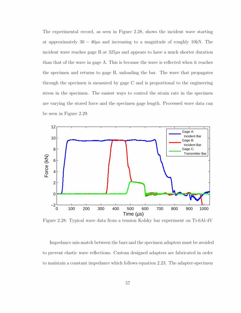
The experimental record, as seen in Figure 2.28, shows the incident wave starting
at approximately 30 − 40µs and increasing to a magnitude of roughly 10kN. The
incident wave reaches gage B at 325µs and appears to have a much shorter duration
than that of the wave in gage A. This is because the wave is reflected when it reaches
the specimen and returns to gage B, unloading the bar. The wave that propagates
through the specimen is measured by gage C and is proportional to the engineering
stress in the specimen. The easiest ways to control the strain rate in the specimen
are varying the stored force and the specimen gage length. Processed wave data can
be seen in Figure 2.29.
0 100 200 300 400 500 600 700 800 900 1000−2
0
2
4
6
8
10
12
Time (µs)
For
ce (
kN)
Gage A: Incident BarGage B: Incident BarGage C: Transmitter Bar
Figure 2.28: Typical wave data from a tension Kolsky bar experiment on Ti-6Al-4V
Impedance mis-match between the bars and the specimen adapters must be avoided
to prevent elastic wave reflections. Custom designed adapters are fabricated in order
to maintain a constant impedance which follows equation 2.23. The adapter-specimen
57

0
200
400
600
800
1000
1200
1400
Eng
inee
ring
Str
ess
(MP
a)
0
500
1000
1500
2000
Eng
inee
ring
Str
ain
Rat
e (1
/s)
0 20 40 60 80 100 1200
0.02
0.04
0.06
0.08
0.1
0.12
0.14
Eng
inee
ring
Str
ain
Time(µs)
Engineering StressEngineering StrainStrain Rate
Figure 2.29: Reduced wave data from a tension Kolsky bar experiment on Ti-6Al-4V
interface has two materials in parallel with one another, see Figure 2.30. The dynamic
tension specimen grip section is the same width as that of the quasi-static specimen
but 16.3mm in length. This section is used to adhere the specimen to the adapter.
Since the specimen grip and adapter impedances are in parallel, the following rela-
tionship must be maintained to match the bar impedance,
Zb = Za + Zs = ρaAaca + ρsAscs = ρbAbcb, (2.28)
where the subscripts b, a, and s represent the bars, adapters, and specimen, respec-
tively. The adapter can be designed if the material properties of the bars, specimen,
and the adapter are known. In this case, the adapter has outside diameter of 6.35mm,
and is fabricated from 6061-T6 aluminum.
58

Figure 2.30: High strain rate specimen with adapters (a)before and (b)following test-ing
2.5.3 High Strain Rate Shear Testing
The stored-torque Kolsky Bar in Figure 2.26, is used to characterize Ti-6Al-4V in
shear at strain rates above 500s−1. The stored-torsion and direct-tension high strain
rate test techniques are similar with the exception of the wave generation method.
The torsion loading wave is generated by clamping and applying a pre-torque to a
section of the bar, see Figure 2.26. The loading wave is released by fracturing a
pin, as in the tension dynamic tests. This technique is described by Gilat[32]. The
wave amplitude is equal to half the stored torque, T , since the wave propagates both
towards and away from the specimen. The strains in the bar are measured with
full Wheatstone bridges each using four Micro-Measurements 1000Ω strain gages in
positions as shown in Figure 2.32[21]. Gage A is located 1715mm from the specimen
on the incident bar. Gages B and C are are located 385mm from the specimen on
both the incident and transmitter bars, respectively. The shear strain incident wave
59

amplitude, γi, is
γi =Trb
2GbJb
, (2.29)
where, rb is the bar radius, Gb is the shear modulus of the bar material, and Jb is the
polar moment of inertia of the bar. As this wave loads the specimen, a portion of the
torque is transmitted through the specimen. This is proportional to the shear stress
in the specimen. The remaining portion of the torque reflects back and is proportional
to the shear strain rate. The angular velocity, θi, of the end of the incident bar is
found from
θi(t) =1
ρbJbct[TA (t− tA) + TA (t− tA + 2tB)− TB (t + tB)] , (2.30)
where, ρb is the density of the bar material, TA(t) and TB(t) are the torque history in
gage A and B, respectively, and ct is the transverse elastic wave speed which is given
by
ct =
√
Gb
ρb, (2.31)
The angular velocity of the transmitter bar, θt(t), is given by
θt(t) =1
ρbJbct[TC (t− tC)] , (2.32)
where, TC is the torque history in the transmitter bar measured by gage C. The shear
strain rate with respect to time is now
γ(t) =rm
[
θi(t)− θt(t)]
ls, (2.33)
where, rm and ls are the mean gage radius and gage length of the specimen, respec-
tively. The shear strain is found by integrating the strain rate with respect to time.
The shear stress is found from
τ(t) =GbJbrmγt(t)
rbJs
=rmTC(t + tC)
Js
, (2.34)
60

where, Js is the polar moment of inertia of the specimen.
The 22.23mm Kolsky bars are made from 7075-T6 aluminum. The clamped and
free sections of the incident bar are 1227mm and 2283mm, respectively. The transmit-
ter bar is 2026mm long. 20.0V excitation to each bridge is provided from HP3611A
power supplies. This apparatus uses the same signal conditioning used for the direct-
tension Kolsky bar.
Dynamic torsion specimens are similar to the spool specimens used for low strain
rate torsion testing. The major difference between these two specimens are the grip-
ping section. Dynamic specimens have a large round flange as seen in Figure 2.31.
Dynamic specimen flanges are designed to have the same mechanical impedance as the
bars. The flanges are glued into adapters, which cumulatively maintain impedance
using the principles previously stated. In this case
Zb = Za + Zs = ρaJact,a + ρsJsct,s = ρbJbct,b, (2.35)
where, J is the polar moment of inertia and the subscripts b, a, and s represent the
bars, adapters, and the specimen, respectively.
Figure 2.31: Comparison of the grip sections between the low and high strain rateshear specimens
61
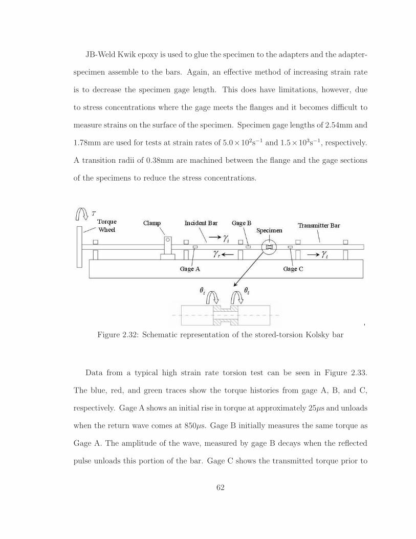
JB-Weld Kwik epoxy is used to glue the specimen to the adapters and the adapter-
specimen assemble to the bars. Again, an effective method of increasing strain rate
is to decrease the specimen gage length. This does have limitations, however, due
to stress concentrations where the gage meets the flanges and it becomes difficult to
measure strains on the surface of the specimen. Specimen gage lengths of 2.54mm and
1.78mm are used for tests at strain rates of 5.0×10²s−1 and 1.5×10³s−1, respectively.
A transition radii of 0.38mm are machined between the flange and the gage sections
of the specimens to reduce the stress concentrations.
Figure 2.32: Schematic representation of the stored-torsion Kolsky bar
Data from a typical high strain rate torsion test can be seen in Figure 2.33.
The blue, red, and green traces show the torque histories from gage A, B, and C,
respectively. Gage A shows an initial rise in torque at approximately 25µs and unloads
when the return wave comes at 850µs. Gage B initially measures the same torque as
Gage A. The amplitude of the wave, measured by gage B decays when the reflected
pulse unloads this portion of the bar. Gage C shows the transmitted torque prior to
62

specimen failure at around 800µs. Dynamic torque equilibrium can be evaluated by
comparing of torques measured by gages B and C at approximately 750µs.
0 250 500 750 1000 1250−25
0
25
50
75
100
125
150
175
Time (µs)
Tor
que
(Nm
)
Gage A: Incident BarGage B: Incident BarGage C: Transmitter Bar
Figure 2.33: Typical wave data from a torsion Kolsky bar experiment on Ti-6Al-4V
Processed data for the test in Figure 2.33 can be seen in Figure 2.34. These data
show the shear stress in blue which, initially, accumulates slowly due to the rise time
of the incident wave. The yield point of the material can coincides with the rapid
change in slope of the stress. Shear strain is represented in green and shows slow
accumulation in strain initially but then becomes constant at approximately 30µs.
Shear strain rate, shown in red, also shows an initially slow rise followed by a leveling
off when equilibrium is reached.
63

0
150
300
450
600
750
She
ar S
tres
s (M
Pa)
0
500
1000
1500
2000
2500
She
ar S
trai
n R
ate
(1/s
)
0 10 20 30 40 50 60 700
0.02
0.04
0.06
0.08
0.1
She
ar S
trai
n
Time(µs)
Shear StressShear StrainShear Strain Rate
Figure 2.34: Reduced wave data from a torsion Kolsky bar experiment on Ti-6Al-4V
2.6 Elevated and Low Temperature Testing Techniques
Titanium used in aerospace applications can experience various operating temper-
atures. At altitude, aircraft engine parts outside of the hot section can see subzero
temperatures. Ti-6Al-4V normal operating temperatures can reach as high as 400C.
A blade-out event leads to large material deformation at high strain rates. Adiabatic
heating takes place under these conditions and temperature increases of 200C are
common. A part at an operating temperature of 400C can reach temperatures of
600C with adiabatic heating. Because of this, the test plan includes experiments at
−50C, 200C, 400C, and, 600C.
Elevated temperature tests are performed using a furnace attached to the hy-
draulic load frame described in section 2.4. The furnace described in depth in Chapter
6, is used for all tension, compression, and shear testing at 200C, 400C, and, 600C.
Digital image correlation is used to measure and record displacements and strains on
the surface of the specimen. Omega, K-type thermocouples, which have an operating
64

range of −200C to 1350C. Temperature data are recorded at 1Hz and compiled for
later analysis.
Tension, compression, and shear cryogenic tests are also performed on the hy-
draulic load frame. Liquid nitrogen is sprayed inside the Styrofoam chamber seen in
Figure 2.35(a), to reach −50C. K-type thermocouples are used to record the tem-
perature of the specimen at a sampling rate of 1Hz. Fog within the chamber makes it
impossible to use DIC for low temperature tests. The load frame’s LVDT and RVDT
are susceptible to compliance errors. An Epsilon miniature axial extensometer model
number 3442-004M050-HT1 is used to measure strain during low temperature tensile
tests. The extensometer, seen in Figure 2.35(b), attaches directly to the specimen
and has a 4mm initial gage length. Compression displacements are measured with an
LVDT located on the compression platens, see in Figure 2.35(b). Rotations in torsion
tests are measured with an RVDT located on grips attached to the spool specimen as
seen in Figure 2.36. The effect of compliance is minimized since these measurements
are taken close to the specimen.
Elevated and low temperature tests provide a more complete description of the
plastic deformation material response under actual operating conditions. Data from
these tests are presented and discussed in Chapter 3.
65

(a) (b)
Figure 2.35: Cryogenic chamber and test setup for tension and compression testingof Ti-6Al-4V (a)Cryogenic testing chamber, (b)Tension and compression setup
(a) (b)
Figure 2.36: Gripping fixture used for cryogenic torsional testing of Ti-6Al-4V(a)Fixture drawing, (b)Test setup
66

2.7 Digital Image Correlation
Digital Image Correlation (DIC) has revolutionized strain measurement in exper-
imental mechanics by allowing researchers to capture full field strains on the surface
of a specimen. An in depth review of this measurement technique is presented by
Sutton, Orteu, and Schreier[25]. The three dimensional DIC system uses two cameras
to track displacements on the surface of a deforming specimen. Strains are calculated
from the tabulated displacements. Although there are several commercial systems in
use, Correlated Solutions VIC-3D 2010 is used here[33].
The three dimensional DIC system is pre-calibrated by photographing a panel
with known grid spacing with both cameras. This creates a three dimensional world
coordinate system. The system takes two synchronized images of a speckle patterned
specimen as seen in Figure 2.37(a). The software algorithm first discretizes the images
into n × n pixel subsets. The gray scale values within the subsets are used to track
the displacements of specimen. Once the displacements are known they are then used
to calculate strains using one of several available strain tensor definitions.
Multiple post processing methods are available including: data extraction at a
point, averaged within a box, or by a virtual extensometer. Data extracted at a
point are useful in tracking the strain state at a the specimen’s fracture location. A
virtual extensometer averages strain over its initial gage. The extensometer is useful
for comparing DIC data to data acquired using more traditional instruments such
as the mechanical extensometer. Average data within a box can also be extracted .
Data extracted at a point or within a box includes ǫxx, ǫyy, ǫxy, ǫ1, ǫ2, x-displacement
(u), y-displacement (v) and z-displacement (w).
67
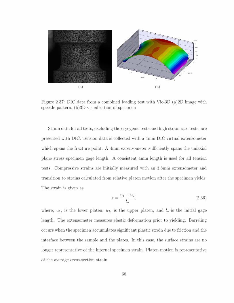
(a) (b)
Figure 2.37: DIC data from a combined loading test with Vic-3D (a)2D image withspeckle pattern, (b)3D visualization of specimen
Strain data for all tests, excluding the cryogenic tests and high strain rate tests, are
presented with DIC. Tension data is collected with a 4mm DIC virtual extensometer
which spans the fracture point. A 4mm extensometer sufficiently spans the uniaxial
plane stress specimen gage length. A consistent 4mm length is used for all tension
tests. Compressive strains are initially measured with an 3.8mm extensometer and
transition to strains calculated from relative platen motion after the specimen yields.
The strain is given as
ǫ =u1 − u2
lo, (2.36)
where, u1, is the lower platen, u2, is the upper platen, and lo is the initial gage
length. The extensometer measures elastic deformation prior to yielding. Barreling
occurs when the specimen accumulates significant plastic strain due to friction and the
interface between the sample and the plates. In this case, the surface strains are no
longer representative of the internal specimen strain. Platen motion is representative
of the average cross-section strain.
68

Shear strain is calculated from three dimensional displacements of points at the
upper and lower regions of the specimen gage section. These data are used with the
law of cosines to calculate the relative angle of rotation between the top and bottom
points as (equation 2.5). The relative angle of twist is proportional to shear strain.
Although DIC data was acquired for the high strain rate tests it was only used for
comparison purposes. High strain rate data reported data in Chapter 3 is measured
using the techniques outlined in Section 2.5 since the strain gages have significantly
better temporal resolution.
Several camera setups spanning a wide range of frame rates are available at the
DMML. For strain rates lower than 1.0×10⁻²s−1, Point Gray Research GRAS-20S4M-
C cameras are used. The cameras acquire images at frame rates up to 19fps at
1624 × 1224 resolution. Either Schneider 35mm or Sigma 50mm lenses are used
with the cameras. Photron MC2 cameras are used at strain rates of 1.0s−1. These
are capable of 2000fps at 512 × 512 resolution. Photron SA1.1 cameras are used
for strain rates at and above 500s−1. These cameras acquire 1024 × 1024 resolution
images at a frame rate of 5400fps. Higher frame rates can be achieved at reduced
resolution. A common frame rate for tests under this project is between 125, 000fps
and 250, 000fps. Either 90mm or 180mm Tamron lenses are used with the Photron
SA1.1 cameras.
DIC provides substantial advantages over classic strain measurement instruments
such as mechanical extensometers or strain gages. Strain gages are cumbersome to
install and are limited to strains of less than 8%. Mechanical extensometers are
easy to use, however they are unable to capture strain localizations. Differences in
stress strain curves measured by the load frame’s LVDT and RVDT are compared
69

to DIC measurements in Figure 2.38. The strain values from these two sources are
considerably different because the DIC measurement is not subjected to compliance
errors. This is especially apparent in the compression data due to the large required
forces which result in more compliance.
0 0.05 0.1 0.15 0.2 0.25 0.3 0.350
500
1000
1500
2000
Strain
Str
ess
(MP
a)
Tension (DIC)Tension (Machine LVDT)Compression (DIC)Compression (Machine LVDT)Torsion (DIC)Torsion (Machine RVDT)
Figure 2.38: Strain measurement comparison between digital image correlation andthe load frame measurement
70

Chapter 3: Plastic Deformation of Ti-6Al-4V Experimental
Results and Discussion
Experimental results generated during the plastic deformation test series, de-
scribed in Table 2.1, are presented here. Quasi-static and high strain rate tension,
compression, and torsion (shear) test data are presented. Data from tension speci-
mens oriented in several directions within the plate and tests conducted at various
temperatures are also presented. All plates tested show notably different plastic defor-
mation characteristics when the data is compared. In order to keep each plate easily
identifiable within the presented plots, a color scheme of blue, red, green, and black
is used for plate 1, 2, 3, and 4, respectively. Different orientations and temperatures
are differentiated with line types or shades. To allow for an easier discussion, tension
and compression data from plate 4 in the rolled direction at a strain rate of 1.0s−1
at room temperature is set as the baseline. Data spread for each test configurations
can be seen in Appendix A. Representative curves from each of the tests are selected
and presented here.
3.1 Experimental Results from the 2.29mm Plate Stock
Plastic deformation data from tests on a 2.29mm thick Ti-6Al-4V plate, labeled
plate 1, are presented here. The plate, purchased from Tri-Tech, was rolled at RMI
71

Titanium and conforms to AMS-4911 Standards. The test methods described in
Chapter 2 were used to generate the following data. Data from this specific plate is
presented here and compared to the other plate stocks in Section 3.5.
3.1.1 Strain Rate Test Series Results
Plate 1 tension stress strain curves at two different strain rates are presented in
Figure 3.1. The plate is clearly rate sensitive for both yield and flow stresses. Fracture
strain in Figure 3.1 look similar at both rates. Strain hardening and fracture strain
at 1.0s−1 and 662s−1 are also similar. Results of the compression tests on plate 1 at
two different strain rates can be seen in Figure 3.2. The material displays strain rate
sensitivity for yield and flow stresses and fracture strains. Compression hardening
characteristics are similar at strain rates of 1.0s−1 and 1393s−1.
0 0.02 0.04 0.06 0.08 0.1 0.12 0.14 0.16 0.18 0.20
200
400
600
800
1000
1200
1400
1600
True Strain
Tru
e S
tres
s (M
Pa)
1.0s−1
662s−1
Figure 3.1: Tension strain rate dependence for plate 1
72

0 0.05 0.1 0.15 0.2 0.25 0.3 0.35 0.40
500
1000
1500
2000
True Strain
Tru
e S
tres
s (M
Pa)
1.0s−1
1393s−1
Figure 3.2: Compression strain rate dependence plate 1
3.1.2 Specimen Orientation Test Series Results
Anisotropy test series data for plate 1 in tension can be seen in Figure 3.3. The
data shows similar yield and plastic deformation characteristics in the rolled and
transverse (90) directions. The 45 data have a similar yield point but different
hardening characteristics and lower flow stresses.
0 0.02 0.04 0.06 0.08 0.1 0.12 0.14 0.16 0.18 0.20
200
400
600
800
1000
1200
1400
True Strain
Tru
e S
tres
s (M
Pa)
Rolled Direction
45o From Rolled
90o From Rolled
Figure 3.3: Tension anisotropy data for plate 1
73

3.2 Experimental Results from the 3.56mm Plate Stock
Plastic deformation data from a 3.56mm thick Ti-6Al-4V plate, labeled plate 2, are
presented here. The plate, also purchased from Tri-Tech and was rolled at TIMET,
conforms to AMS-4911 standards. The test methods described in Chapter 2 are used
to generate the following data. Data from this specific plate are presented here and
compared to the other plate stocks in Section 3.5.
3.2.1 Strain Rate Test Series Results
Tension and compression stress strain curves for plate 2 are presented in Figure
3.4 and Figure 3.5, respectively. In both cases, the material displays rate dependent
yield and flow stresses and fracture strains. Yield and flow stresses increase with
increasing strain rate while the fracture strains decrease.
0 0.02 0.04 0.06 0.08 0.1 0.12 0.14 0.16 0.18 0.20
200
400
600
800
1000
1200
1400
1600
True Strain
Tru
e S
tres
s (M
Pa)
1.0s−1
640s−1
Figure 3.4: Tension strain rate dependence for plate 2
74

0 0.05 0.1 0.15 0.2 0.25 0.3 0.35 0.40
500
1000
1500
2000
True Strain
Tru
e S
tres
s (M
Pa)
1.0s−1
1744s−1
Figure 3.5: Compression strain rate dependence for plate 2
3.2.2 Specimen Orientation Test Series Results
Tension data from specimens fabricated in three orientations within plate 2 can
be seen in Figure 3.6. This plate shows similar yield, plastic deformation, hardening,
and fracture characteristics for all orientations evaluated. According to the data in
Figure 3.6 the material appears to be isotropic.
0 0.02 0.04 0.06 0.08 0.1 0.12 0.14 0.16 0.18 0.20
200
400
600
800
1000
1200
1400
True Strain
Tru
e S
tres
s (M
Pa)
Rolled Direction
45o From Rolled
90o From Rolled
Figure 3.6: Tension anisotropy data for plate 2
75

3.3 Experimental Results from the 6.35mm Plate Stock
The 6.35mm thick Ti-6Al-4V plate, labeled plate 3, was extensively tested previously[12]
Additional tests are presented here. The plate was purchased from Tri-Tech and rolled
at Allegheny Ludlum to conform to AMS-4911 standards. The test methods described
in Chapter 2 were used to generate the data. A comparison of plate 3 to the other
stocks is presented in Section 3.5.
3.3.1 Temperature Test Series Results
Tension test data at −50oC, 200oC, 400oC, and 600oC are presented in Figure 3.7.
The stress monotonically decreases with increasing temperature. Strain hardening
is also clearly effected by the change in temperature. The data shows an increasing
fracture strains at elevated temperatures indicating an increase in ductility. The
−50oC tests show in an increase in flow stresses and a reduction in fracture strain
implying a brittling effect of the material at lower temperatures.
0 0.05 0.1 0.15 0.2 0.25 0.30
200
400
600
800
1000
1200
1400
True Strain
Tru
e S
tres
s (M
Pa)
25oC
200oC
400oC
600oC
−50oC
Figure 3.7: Tension temperature test series data for plate 3
76
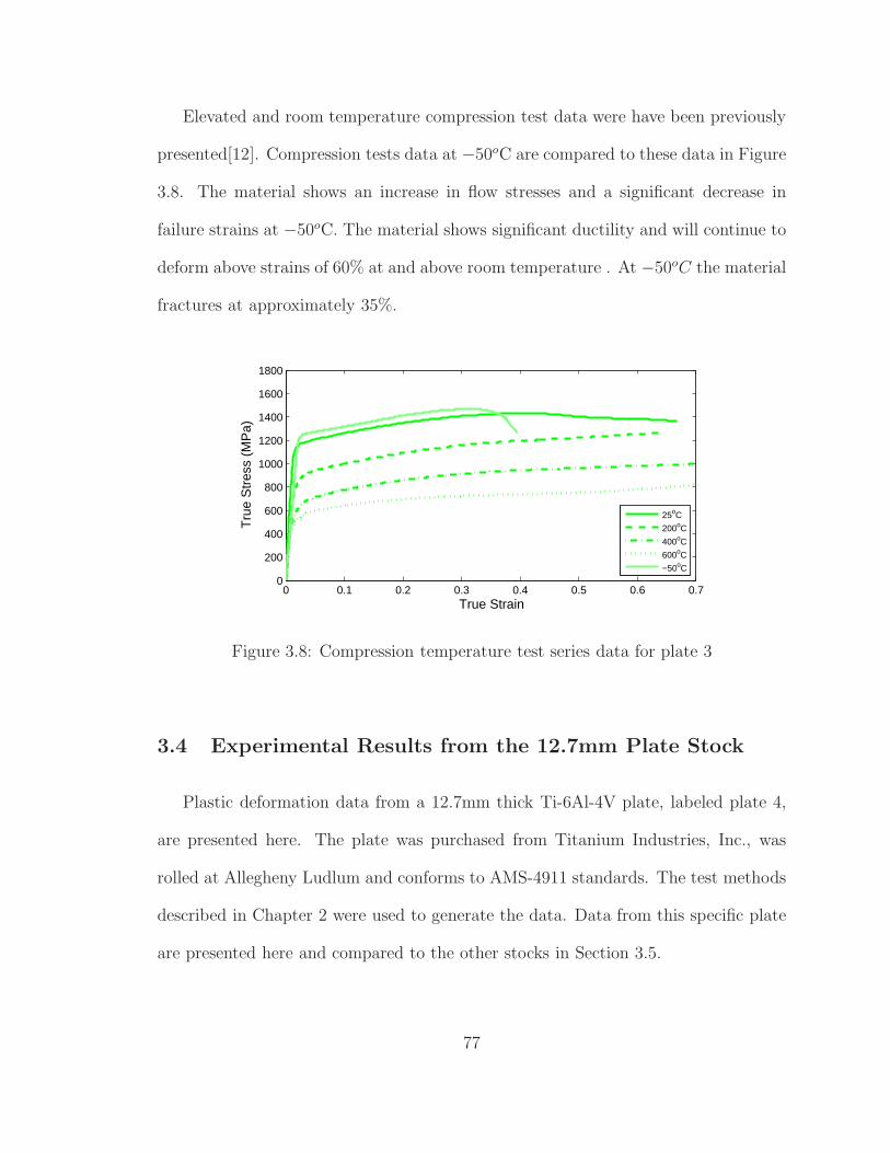
Elevated and room temperature compression test data were have been previously
presented[12]. Compression tests data at −50oC are compared to these data in Figure
3.8. The material shows an increase in flow stresses and a significant decrease in
failure strains at −50oC. The material shows significant ductility and will continue to
deform above strains of 60% at and above room temperature . At −50oC the material
fractures at approximately 35%.
0 0.1 0.2 0.3 0.4 0.5 0.6 0.70
200
400
600
800
1000
1200
1400
1600
1800
True Strain
Tru
e S
tres
s (M
Pa)
25oC
200oC
400oC
600oC
−50oC
Figure 3.8: Compression temperature test series data for plate 3
3.4 Experimental Results from the 12.7mm Plate Stock
Plastic deformation data from a 12.7mm thick Ti-6Al-4V plate, labeled plate 4,
are presented here. The plate was purchased from Titanium Industries, Inc., was
rolled at Allegheny Ludlum and conforms to AMS-4911 standards. The test methods
described in Chapter 2 were used to generate the data. Data from this specific plate
are presented here and compared to the other stocks in Section 3.5.
77

3.4.1 Strain Rate Test Series Results
Plate 4 shows significant strain rate dependence in tension, compression, and
shear. Tension strain rate test series data can be seen in Figure 3.9. Yield and
flow stresses increase with increasing strain rate, however, the failure strains are
significantly decrease at and above 1.0s−1. The dynamic curves show a different elastic
modulus than the low rate curves. This is due to the fact that elastic modulus cannot
be accurately measured using of a Kolsky bar because dynamic force equilibrium does
not exist early in the test.
0 0.02 0.04 0.06 0.08 0.1 0.12 0.14 0.16 0.18 0.20
500
1000
1500
True Strain
Tru
e S
tres
s (M
Pa)
1.0x10⁻⁴ s−1
1.0x10⁻² s−1
1.0 s−1
640 s−1
1645 s−1
Figure 3.9: Tension strain rate test series data for plate 4
Compression data, shown in Figure 3.10, also exhibits an increase in yield and flow
stresses with increasing strain rate. The initial peak oscillating nature of the high
strain rate data is not material response but error caused by force in equilibrium and
three dimensional wave propagation in the bars. The material also displays decreasing
failure strains in compression, especially at and above 1500s−1. In both tension and
compression, there is a clear change in strain hardening between 1.0 × 10⁻²s−1 at
1.0s−1.
78

0 0.05 0.1 0.15 0.2 0.25 0.3 0.35 0.40
500
1000
1500
2000
True Strain
Tru
e S
tres
s (M
Pa)
1.0x10⁻⁴ s−1
1.0x10⁻² s−1
1.0 s−1
1474s−1
3879s−1
7971s−1
Figure 3.10: Compression strain rate test series data for plate 4
Shear test data, shown in Figure 3.11, also demonstrate strain rate dependence for
yield and flow stresses as well as failure strains. Shear failure strains are similar for
strain rates at and below 1.0s−1, however at strain rates higher than 1.0s−1, failure
strain reduces dramatically.
0 0.02 0.04 0.06 0.08 0.1 0.12 0.14 0.16 0.18 0.20
100
200
300
400
500
600
700
Shear Strain
She
ar S
tres
s (M
Pa)
1.0E−4s−1
1.0E−2s−1
1.0s−1
323s−1
907s−1
Figure 3.11: Shear strain rate test series data for plate 4
79
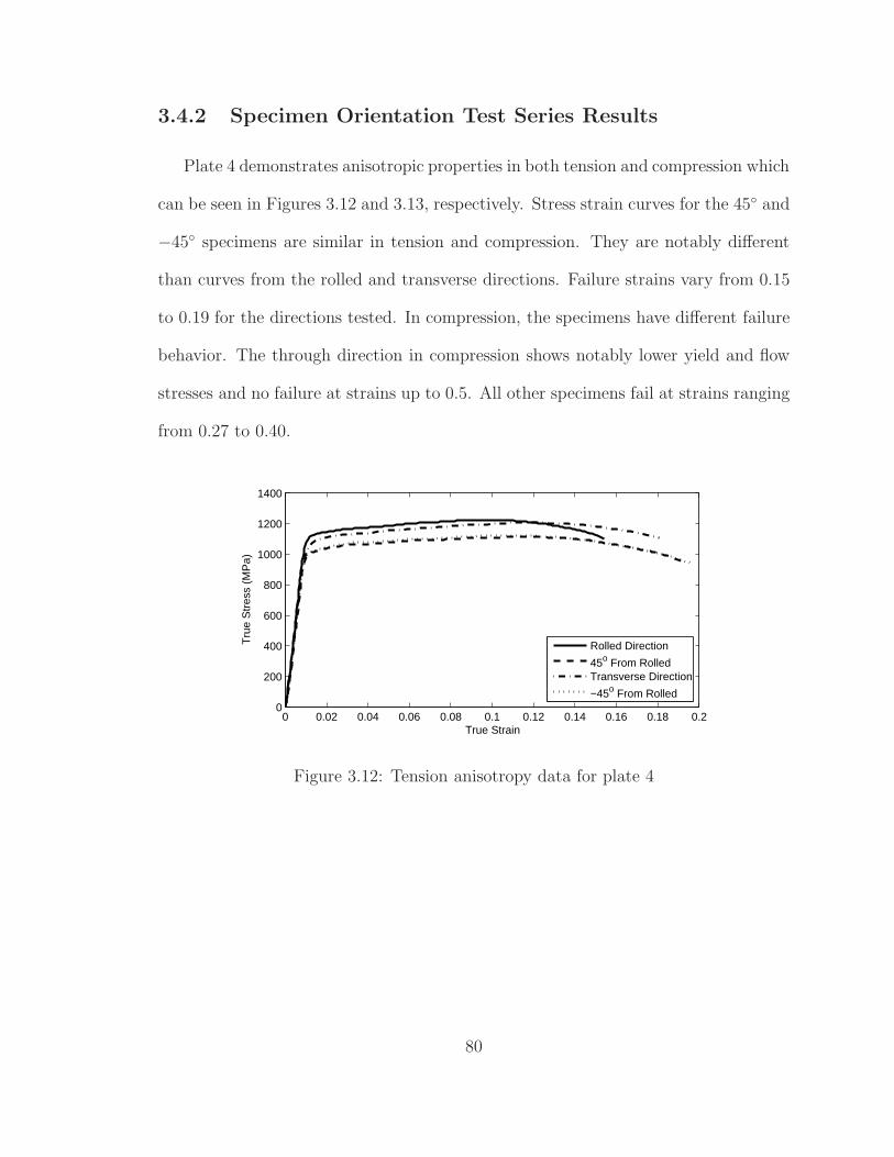
3.4.2 Specimen Orientation Test Series Results
Plate 4 demonstrates anisotropic properties in both tension and compression which
can be seen in Figures 3.12 and 3.13, respectively. Stress strain curves for the 45 and
−45 specimens are similar in tension and compression. They are notably different
than curves from the rolled and transverse directions. Failure strains vary from 0.15
to 0.19 for the directions tested. In compression, the specimens have different failure
behavior. The through direction in compression shows notably lower yield and flow
stresses and no failure at strains up to 0.5. All other specimens fail at strains ranging
from 0.27 to 0.40.
0 0.02 0.04 0.06 0.08 0.1 0.12 0.14 0.16 0.18 0.20
200
400
600
800
1000
1200
1400
True Strain
Tru
e S
tres
s (M
Pa)
Rolled Direction
45o From RolledTransverse Direction
−45o From Rolled
Figure 3.12: Tension anisotropy data for plate 4
80

0 0.05 0.1 0.15 0.2 0.25 0.3 0.35 0.4 0.45 0.50
200
400
600
800
1000
1200
1400
1600
True Strain
Tru
e S
tres
s (M
Pa)
Rolled Direction
45o From RolledTransverse Direction
−45o From RolledThrough Direction
Figure 3.13: Compression anisotropy data for plate 4
3.4.3 Temperature Test Series Results
Plate 4’s tension temperature dependence can be seen in Figure 3.14. The ma-
terial displays monotonically decreasing yield and flow stresses with increasing tem-
perature. There are significant increases in ductility from 25C to 200C and from
400C to 600C. Compression results also display decreasing stresses with increasing
temperature, see Figure 3.15. Unlike in tension, Ti-6Al-4V has a significant increase
in compressive fracture strain between 200C and 400C. Shear test results, see in
Figure 3.16, also display falling stresses with increasing temperature. Ductility in
shear increases with every increased temperature. The cryogenic shear curve displays
a lower shear modulus than the room temperature data. This is due to measurement
error and not a physical property of the material. The displacement between these
tests were not measured using the same method as described in Subsection 2.2.3 and
Section 2.6.
81

0 0.05 0.1 0.15 0.2 0.25 0.30
200
400
600
800
1000
1200
1400
True Strain
Tru
e S
tres
s (M
Pa)
25oC
200oC
400oC
600oC
−50oC
Figure 3.14: Tension temperature dependence for plate 4
0 0.1 0.2 0.3 0.4 0.5 0.6 0.70
200
400
600
800
1000
1200
1400
1600
1800
True Strain
Tru
e S
tres
s (M
Pa)
25oC
200oC
400oC
600oC
−50oC
Figure 3.15: Compression temperature dependence for plate 4
82

0 0.05 0.1 0.15 0.2 0.25 0.3 0.35 0.4 0.45 0.50
100
200
300
400
500
600
700
Shear Strain
She
ar S
tres
s (M
Pa)
25oC
200oC
400oC
600oC
−50oC
Figure 3.16: Shear temperature dependence for plate 4
3.5 Comparison of the Various Plate Stocks Tested
Although all plates are within AMS specifications, they show notably different
plastic deformation characteristics. Differences discussed here are outside of test
data spread and are attributed to differences in plate characteristics.
3.5.1 Tension Comparison
In tension, plate 4 has higher yield and flow stresses compared to plates 1, 2, and
3 see Figure 3.17. These curves are for room temperature tests at a strain rate of
1.0s−1 for specimens fabricated in the rolled direction. Fracture strains are similar
for all plates and range from 0.14 to 0.16. Strain hardening characteristics are similar
for all curves in Figure 3.17.
A complete plate stock comparison for all tensile strain rate dependence tests can
be seen in Figure 3.18. Plate 1’s flow stresses are 6% lower and 6% higher than
baseline (Plate 4 at Room Temperature, 1.0s−1) at 1.0s−1 and 662s−1, respecitvely.
83

0 0.02 0.04 0.06 0.08 0.1 0.12 0.14 0.16 0.18 0.20
200
400
600
800
1000
1200
1400
True Strain
Tru
e S
tres
s (M
Pa)
Plate 1 [0.090in]Plate 2 [0.140in]Plate 3 [0.250in]Plate 4 [0.500in]
Figure 3.17: Comparison of plate 1, 2, 3, and 4 in tension at a strain rate of 1.0s−1,at room temperature, specimens orientated in the rolled direction
Plate 2’s results are similar for flow stresses but display much higher failure strain
at 1.0s−1. Plate 3 at strain rates of 1.0 × 10⁻⁴s−1, 1.0 × 10⁻²s−1, 1.0s−1, 538s−1,
and 1332s−1 the flow stresses are −18%, −9%, −5%, 6%, and 9% different than the
baseline, respectively. Plate 4’s flow stresses are −13%, −10%, 9%, and 13% different
than the baseline at strain rates of 1.0× 10⁻⁴s−1, 1.0× 10⁻²s−1, 640s−1, and 1645s−1,
respectively. Plate 4 exhibits a smaller difference in flow stress between 1.0×10⁻⁴s−1
and 1.0 × 10⁻²s−1 than plate 3. Plates 1 and 3 have similar failure strains between
each of the strain rates. There is a clear change in Plates 2 and 4 at and above 1.0s−1.
Strain hardening is similar for all plates at all strain rates.
Tension data from tests on specimens oriented in various directions withing all four
plates are presented in 3.19. Plate 1’s rolled and transverse flow stresses are about 6%
lower than baseline. Its 45 flow stresses are 16% lower than baseline. All orientations
84
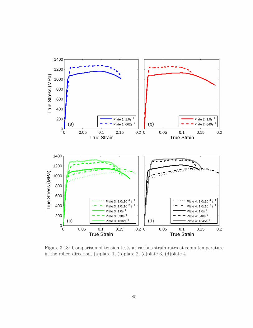
0 0.05 0.1 0.15 0.20
200
400
600
800
1000
1200
1400
Tru
e S
tres
s (M
Pa)
True Strain
(a)Plate 1: 1.0s−1
Plate 1: 662s−1
0 0.05 0.1 0.15 0.2True Strain
(b)Plate 2: 1.0s−1
Plate 2: 640s−1
0 0.05 0.1 0.15 0.20
200
400
600
800
1000
1200
1400
Tru
e S
tres
s (M
Pa)
True Strain
(c)
Plate 3: 1.0x10⁻⁴ s−1
Plate 3: 1.0x10⁻² s−1
Plate 3: 1.0s−1
Plate 3: 538s−1
Plate 3: 1332s−1
0 0.05 0.1 0.15 0.2True Strain
(d)
Plate 4: 1.0x10⁻⁴ s−1
Plate 4: 1.0x10⁻² s−1
Plate 4: 1.0s−1
Plate 4: 640s−1
Plate 4: 1645s−1
Figure 3.18: Comparison of tension tests at various strain rates at room temperaturein the rolled direction, (a)plate 1, (b)plate 2, (c)plate 3, (d)plate 4
85

have similar fracture strains which approximately match the baseline. Flow stresses,
in all three directions, for plate 2 are approximately 8% lower than baseline. All
orientations in this plate have similar fracture strains and are about 19% higher than
baseline. For plate 3, the rolled and transverse directions display similar behaviors and
have 6% and 4% lower flow stresses than the baseline, respectively. ±45 directions
display similar behavior and have about 16% lower flow stress than baseline. Failure
strains all approximately mate the baseline and range from 0.12 to 0.17. Plate 4 data
in the rolled and transverse directions display similar behaviors with an approximate
flow stress of 1226MPa (Tension Baseline). ±45 directions display similar behaviors
and have approximately 10% lower flow stress than the baseline. Excluding the 45
direction in plate 1, strain hardening behavior from all tests in Figure 3.19 are similar.
A comparison of tension tests at various temperatures on specimens fabricated
from plates 3 and 4 are displayed in Figure 3.20. These tests are conducted on rolled
direction specimens at 1.0s−1. The data shows a convergence of material characteris-
tics at and above 200C. Plate 3’s yield and flow stresses at−50C increase more than
those for plate 4. There is also a significantly larger reduction in ductility for plate 3
at this temperature. Both materials become more ductile at higher temperatures.
86

0 0.05 0.1 0.15 0.20
200
400
600
800
1000
1200
1400
Tru
e S
tres
s (M
Pa)
True Strain
(a)
Plate 1 Rolled Direction
Plate 1 45o From Rolled
Plate 1 90o From Rolled
0 0.05 0.1 0.15 0.2True Strain
(b)
Plate 2 Rolled Direction
Plate 2 45o From Rolled
Plate 2 90o From Rolled
0 0.05 0.1 0.15 0.20
200
400
600
800
1000
1200
1400
Tru
e S
tres
s (M
Pa)
True Strain
(c)
Plate 3 Rolled Direction
Plate 3 45o From Rolled
Plate 3 90o From Rolled
Plate 3 135o From Rolled
0 0.05 0.1 0.15 0.2True Strain
(d)
Plate 4 Rolled Direction
Plate 4 45o From Rolled
Plate 4 90o From Rolled
Plate 4 135o From Rolled
Figure 3.19: Comparison of tension tests at various fabrication orientations at roomtemperature and a strain rate of 1.0s−1, (a)Plate 1, (b)Plate 2, (c)Plate 3, (d)Plate 4
87

0 0.05 0.1 0.15 0.2 0.25 0.30
200
400
600
800
1000
1200
1400
True Strain
Tru
e S
tres
s (M
Pa)
P3 25oC
P3 200oC
P3 400oC
P3 600oC
P3 −50oC
P4 25oC
P4 200oC
P4 400oC
P4 600oC
P4 −50oC
Figure 3.20: Comparison of tension tests at various temperatures at a strain rate of1.0s−1 from the rolled direction for plate 3 and 4
3.5.2 Compression Comparison
Compression data at various strain rates from plate 3 and plate 4 are compared in
Figure 3.21. Plates 1 and 2 are not shown since they were only tested in the through
direction. Baseline is described as the room temperature test at 1.0s−1 in the rolled
direction from plate 4.
Plate 3 displays flow stresses that are approximately −21%, −15%, −11%, −1%,
and 1% different from the baseline for strain rates of 1.0 × 10⁻⁴s−1, 1.0 × 10⁻²s−1,
1.0s−1, 1728s−1, and 3022s−1, respecitvely. Plate 4 data differs from the baseline by
−10%, −1%, 13%, and 20% at respective strain rates of 1.0× 10⁻⁴s−1, 1.0× 10⁻²s−1,
1474s−1, and 3879s−1. At low strain rates (≤ 1.0 × 10⁻²s−1), after an approximate
strain of 0.28, plate 4 fails in shear at a 45 degree angle. Plate 3, however, continues
to deform and does not fail below a strain of 0.35. Both plates fail in shear at or below
88

an approximate strain of 0.30 at high strain rates (≥ 1000s−1). In compression, the
strain hardening behavior is similar in all corresponding tests between the two plates.
Both plates have a significant strain hardening change at a strain rate of 1.0s−1
0 0.1 0.2 0.3 0.4 0.50
500
1000
1500
2000
Tru
e S
tres
s (M
Pa)
True Strain
(a)
Plate 3 @ 1.0x10⁻⁴s−1
Plate 3: 1.0x10⁻²s−1
Plate 3: 1.0s−1
Plate 3: 1728s−1
Plate 3: 3022s−1
0 0.1 0.2 0.3 0.4 0.5True Strain
(b)
Plate 4: 10−4s−1
Plate 4: 10−2s−1
Plate 4: 1.0s−1
Plate 4: 1474s−1
Plate 4: 3879s−1
Plate 4: 7971s−1
Figure 3.21: Comparison of compression testing at various strain rates from the rolleddirection for plates 3(a) and 4(b)
Stress strain curves from specimens fabricated in the thickness direction of the
different plate stocks are compared in Figure 3.22. These tests are conducted at room
temperature at a strain rate of 1.0s−1. These data imply that all the plate stocks have
similar characteristics at this strain rate. Data from specimens orientated in several
directions within plates 3 and 4 are shown in Figure 3.23. A comparison of these data
shows that they have strongly anisotropic characteristics. Ductility in the through
direction for plate 3 is similar to the transverse direction but much lower than the
rolled, ±45. Flow stresses for this plate in the rolled and ±45 directions are lower
than those in the transverse. Plate 4 exhibits very ductile behavior only in the through
89

thickness orientation. Flow stresses in the through directions are approximately 5%
lower than the others. Differences in these plates fall well outside of the data spread.
Data spread plots for all plastic deformation testing can be found in Appendix A.
Plate 3 is strongly anisotropic in compression and it’s trends do not follow those
seen in tension. Plate 4 compression data are more isotropic than plate 3, how-
ever, there are some notable differences in properties between the tested orientations.
Rolled and transverse, and ±45 have similar properties with only a slight strain hard-
ening differences between the two groups. The through direction has a much higher
ductility and lower flow stress. The through direction for plates 3 and 4, however,
does not agree with the in-plane compressive behavior for these plates and therefore
only gives an incomplete comparison.
0 0.05 0.1 0.15 0.2 0.25 0.3 0.35 0.4 0.45 0.50
200
400
600
800
1000
1200
1400
1600
True Strain
Tru
e S
tres
s (M
Pa)
Plate 1 [0.090in]Plate 2 [0.140in]Plate 3 [0.250in]Plate 4 [0.500in]
Figure 3.22: Comparison of plates 1, 2, 3, and 4 in compression at a strain rate of1.0s−1 in the through thickness direction
90

0 0.1 0.2 0.3 0.4 0.50
200
400
600
800
1000
1200
1400
1600
Tru
e S
tres
s (M
Pa)
True Strain
(a)
Plate 3 Rolled Direction
Plate 3 45o From Rolled
Plate 3 90o From Rolled
Plate 3 135o From RolledPlate 3 Through Direction
0 0.1 0.2 0.3 0.4 0.5True Strain
(b)
Plate 4 Rolled Direction
Plate 4 45o From Rolled
Plate 4 90o From Rolled
Plate 4 135o From RolledPlate 4 Through Direction
Figure 3.23: Comparison of plate 3(a) and 4(b) in compression at various fabricationorientations at room temperature and a strain rate of 1.0s−1
A comparison of data from tests at various temperatures on plates 3 and 4 are
presented in Figure 3.24. These tests were conducted on samples oriented in the rolled
direction at 1.0s−1. Tension stress strain curves converge at 200C, however, compres-
sion curves do not converge until 600C. Plate 3’s compressive flow stress increase
in cryogenic tests is smaller in compression than in tension. Plate 4 becomes much
more ductile above 200C. Plate 3 is very ductile, at and above room temperature,
but it displays a brittle failure at −50C.
91

0 0.1 0.2 0.3 0.4 0.5 0.6 0.70
200
400
600
800
1000
1200
1400
1600
True Strain
Tru
e S
tres
s (M
Pa)
P3 25oC
P3 200oC
P3 400oC
P3 600oC
P3 −50oC
P4 25oC
P4 200oC
P4 400oC
P4 600oC
P4 −50oC
Figure 3.24: Comparison of plate 3 and 4 in compression at various temperatures inthe rolled direction at 1.0s−1
3.6 Johnson-Cook Plasticity Model Parameter Determina-
tion
In this section Johnson-Cook Plasticity material parameters are determined from
previously presented Plate 4 data. Since the plastic deformation characteristics in
tension, compression, and shear are considerably different, each loading condition
should have it’s own unique set of parameters. Parameters presented here are found
from rolled direction tension data from plate 4. These parameters are compared to
those found previously. This includes parameters for the plate 3 stock[12]. Previously
found tabulated parameters can be seen in Table 1.2.
Coefficients within the first set of brackets in Equation 1.1 are found when the
second and third set of brackets are both equal to one. The second bracket is one
when the strain rate is equal to the reference strain rate (ǫo = 1.0s−1). The third
92

bracket is equal to one when the material temperature is equivalent to the reference
temperature (T = 25C). Equation 1.1 reduces to,
σ = [A+Bǫn] . (3.1)
A is determined from the yield point of the material. B and n are found with a
curve fit of the data. These parameters are determined to be 1062MPa, 431MPa,
and 0.50, respectively. Effective stress versus equivalent plastic strain curves for each
set of the JC model parameters is compared with the test data in Figure 3.25. The
Johnson parameters clearly underestimate yield and flow stresses but it has similar
strain hardening. The Yatnalkar model is comparable in yield and flow stresses as
well as strain hardening. The Lesuer model fits the data reasonably well, however,
the fit diverges at low and high strains. Finally, the Milani model captures the yield
stress but overestimates flow stress and strain hardening for the Plate 4 data.
0 0.02 0.04 0.06 0.08 0.1 0.12600
700
800
900
1000
1100
1200
1300
1400
Equivalent Plastic Strain
Effe
ctiv
e S
tres
s (M
Pa)
Plate 4 Tension DataLesuer ParametersJohnson ParametersYatnalkar ParametersMilani ParametersHammer Parameters
Figure 3.25: Comparison of several Johnson-Cook constitutive model parameters toplate 4 test data
93

The parameter, C, is determined by curve fitting normalized stresses at the dif-
ferent strain rates. Stress magnitudes, σ, are taken from each strain rate at a strain
of 5%. These values are then normalized to the reference strain rate (1.0s−1) stress
magnitude. Equation 1.1 becomes,
σ
σr
=
[
1 + C ln
(
ǫ
ǫo
)]
(3.2)
C is determined through a linear curve fit to the stresses versus logarithmic strain
rate. The normalization value is
σr = [A+ Ben]
[(
T − Tr
Tm − Tr
)m]
(3.3)
The test data with various model parameter fits are plotted in Figure 3.26. The
Lesuer and Johnson models predict similar strain rate dependence as Plate 4. The
Yatnalkar parameters overestimate the strain rate sensitivity while the Milani param-
eters greatly underestimate it.
The JC temperature parameter, m, is determined from normalized stresses at
various temperatures at a strain rate of 1.0s−1. The stress magnitudes are taken at
5% strain temperatures of 25C to 600C. The stresses are normalized in by
σ
σr
=
[
1−(
T − Tr
Tm − Tr
)m]
, (3.4)
where the normalized stress is taken as
σr = [A+Bǫn]
[
1 + C ln
(
ǫ
ǫo
)]
(3.5)
A curve fit of the normalized stresses yields 0.69 for the temperature parameter. Nor-
malized stress data are plotted with several JC model parameters in Figure 3.27. The
Leseur, Johnson, and Milani parameters underestimate the effect of the temperature
on the stress.
94

10−5
10−3
10−1
101
103
105
800
900
1000
1100
1200
1300
1400
1500
Strain Rate (s−1)
Effe
ctiv
e S
tres
s (M
Pa)
Plate 4 Tension DataLesuer ParametersJohnson ParametersYatnalkar ParametersMilani ParametersHammer Parameters
Figure 3.26: Comparison of several Johnson-Cook constitutive model parameters toplate 4 tension strain rate data extracted at a strain of 5% at room temperature inthe rolled direction
0 0.05 0.1 0.15 0.2 0.25 0.3 0.35 0.4 0.45 0.50.4
0.5
0.6
0.7
0.8
0.9
1
T*
σ/m
ax(σ
)
Plate 4 Tension DataLesuer ParametersJohnson ParametersMilani ParametersHammer Parameters
Figure 3.27: Comparison of several Johnson-Cook constitutive model parameters toplate 4 temperature data in tension at a strain rate of 1.0s−1
95
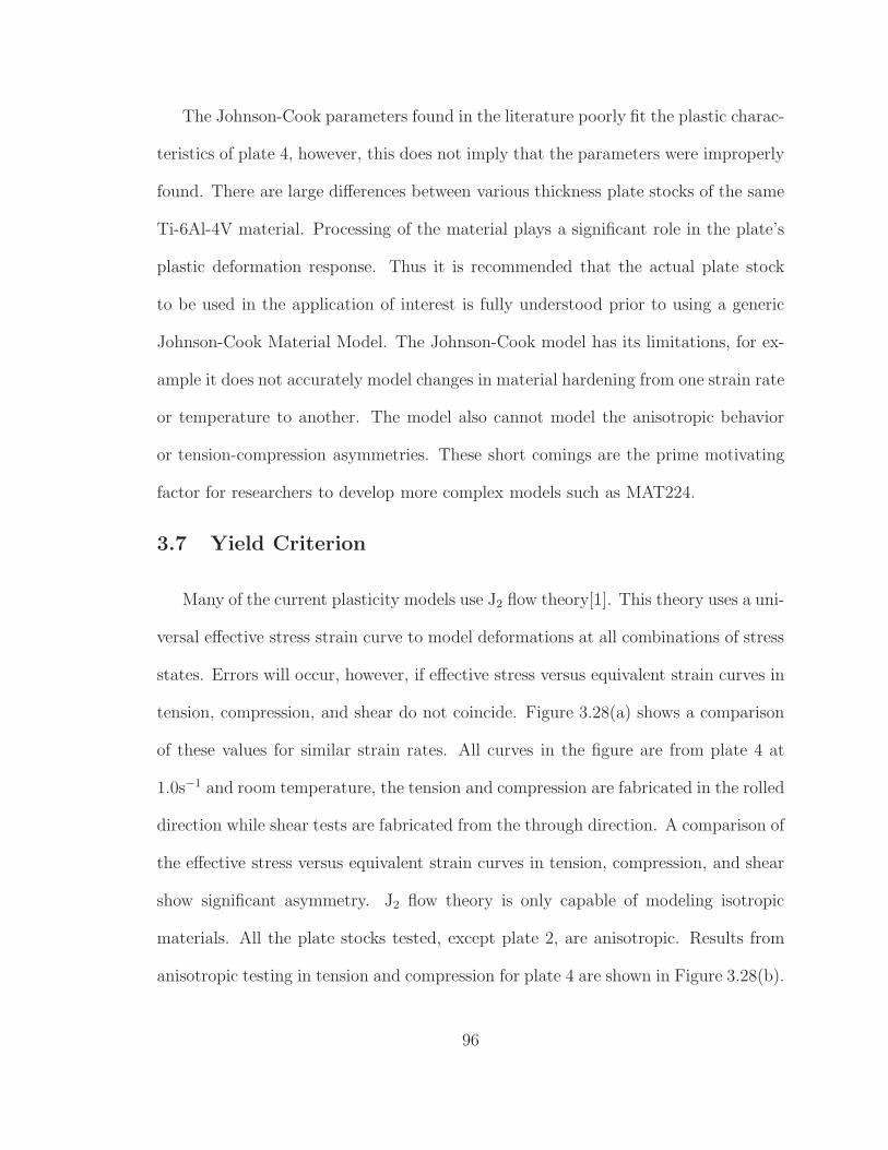
The Johnson-Cook parameters found in the literature poorly fit the plastic charac-
teristics of plate 4, however, this does not imply that the parameters were improperly
found. There are large differences between various thickness plate stocks of the same
Ti-6Al-4V material. Processing of the material plays a significant role in the plate’s
plastic deformation response. Thus it is recommended that the actual plate stock
to be used in the application of interest is fully understood prior to using a generic
Johnson-Cook Material Model. The Johnson-Cook model has its limitations, for ex-
ample it does not accurately model changes in material hardening from one strain rate
or temperature to another. The model also cannot model the anisotropic behavior
or tension-compression asymmetries. These short comings are the prime motivating
factor for researchers to develop more complex models such as MAT224.
3.7 Yield Criterion
Many of the current plasticity models use J2 flow theory[1]. This theory uses a uni-
versal effective stress strain curve to model deformations at all combinations of stress
states. Errors will occur, however, if effective stress versus equivalent strain curves in
tension, compression, and shear do not coincide. Figure 3.28(a) shows a comparison
of these values for similar strain rates. All curves in the figure are from plate 4 at
1.0s−1 and room temperature, the tension and compression are fabricated in the rolled
direction while shear tests are fabricated from the through direction. A comparison of
the effective stress versus equivalent strain curves in tension, compression, and shear
show significant asymmetry. J2 flow theory is only capable of modeling isotropic
materials. All the plate stocks tested, except plate 2, are anisotropic. Results from
anisotropic testing in tension and compression for plate 4 are shown in Figure 3.28(b).
96

These results indicate that J2 plasticity theory is unable to adequately characterize
the material.
0 0.05 0.1 0.15 0.2 0.25 0.30
200
400
600
800
1000
1200
1400
1600(a)
Equivalent Strain
Effe
ctiv
e S
tres
s (M
Pa)
TensionCompressionTorsion
0 0.1 0.2 0.3 0.4 0.50
200
400
600
800
1000
1200
1400
1600
Equivalent Strain
(b)
Tension: Rolled Direction
Tension: 45o From RolledTension: Transverse Direction
Tension: −45o From RolledCompression: Rolled Direction
Compression: 45o From RolledCompression: Transverse Direction
Compression: −45o From RolledCompression: Through Direction
Figure 3.28: Plate 4 (a)asymmetry and (b)anisotropy test data
3.8 Conclusions
Test data for several Ti-6Al-4V plates are presented here. Tests were carried
out in tension, compression, and shear at quasi-static and dynamic loading rates.
The Material has been tested in several orientations with in the plate. Multiple
temperatures were also tested.
The response of Ti-6Al-4V is highly dependent on loading rate as seen by the flow
stresses in Figure 3.29. Additionally, strain hardening and failure strains can also be
rate dependent. As strain rate increases, the yield and flow stress also increase while
failure strains decrease. There is a notable change in strain hardening at and above
1.0s−1, in compression.
Excluding Plate 2, the material shows significant anisotropic characteristics. In
compression, Plates 3 and 4 show considerably different anisotropic characteristics. In
97

10−5
10−3
10−1
101
103
105
0
250
500
750
1000
1250
1500
1750
2000
Strain Rate (s−1)
Effe
ctiv
e S
tres
s (M
Pa)
Plate 1 CompressionPlate 1 TensionPlate 2 CompressionPlate 2 TensionPlate 3 CompressionPlate 3 TensionPlate 4 CompressionPlate 4 TensionPlate 4 Shear
Figure 3.29: Strain rate dependence of various plate stocks of Ti-6Al-4V in tension,compression, and shear at strains of 5%
tension, the rolled and transverse stress strain curves from plates 3 and 4 are similar.
This is also the case for the ±45 stress strain curves. There is a notable difference
between tensile, compressive, and shear yield and flow stresses, failure strains, and
strain hardening.
Plates 3 and 4 have significant temperature dependence between −50C to 600C,
as seen in Figure 3.30. As the temperature increases the yield and flow stresses
decrease while failure strains increase. Plate 3 has a significantly higher increase in
flow stress between room temperature and −50C than Plate 4 does. In tension, the
stress strain curves of plates 3 and 4 converge at 200C while in compression, they
do not converge until above 600C. In compression, plate 3 experiences shear failure
at −50C while plate 4 experiences shear fracture at temperatures below 400C.
Although the four different plate stocks researched here are compliant with the
same Aerospace Materials Standards, they have significant differences in plastic de-
formation characteristics. These plates have large differences in strength, failure
98

−100 0 100 200 300 400 500 6000
200
400
600
800
1000
1200
1400
1600
Temperature(oC)
Effe
ctiv
e S
tres
s (M
Pa)
Plate 3 CompressionPlate 3 TensionPlate 4 CompressionPlate 4 TensionPlate 4 Shear
Figure 3.30: Temperature dependence of various plate stocks of Ti-6Al-4V in multipleloading conditions
strains, anisotropy, strain hardening, and failure type. While modeling this material,
care should be taken to ensure that appropriate material properties are used for the
specific plate stock being utilized. The material also has different characteristics in
tension, compression, and shear. Ti-6Al-4V is, for the most part, anisotropic. These
properties, however, differ under tension, compression and with the material stock.
Strain hardening, failure strain, failure type, yield stress, and flow stress are all depen-
dent on strain rate. Any material model that is used to model the dynamic behavior
of Ti-6Al-4V must be able to accurately model the strain rate reported characteristics.
99

Chapter 4: Ductile Fracture Experimental Results and
Construction of the Fracture Locus for Ti-6Al-4V
Experimental results from the ductile fracture testing described in Section 2.3 are
presented here. Tension test results for plane stress, axisymmetric, and plane strain
specimens, and combined loading axial-torsional test results are shown. Specimens
are fabricated from plate 4 due to size restrictions of plates 1, 2 and 3. Engineering
stress (or force normalized by initial area) and engineering strain are reported for all
tension geometries. A 4mm virtual extensometer is used to measure strain for each
tension experiment presented here. Data spread for each geometry tested can be seen
in Appendix B. Representative curves from each of the tests have been selected and
presented here.
4.1 Plane Stress Experiments
The plane stress specimens, discussed in Chapter 2, are have a thin, flat, smooth
or notched geometry (see Table 2.2). These specimens have stress triaxialities ranging
from 0.400 to 0.583. Lode parameters range from 0.014 to 0.845.
Results from the plane stress tension tests are presented in Figure 4.1. The smooth
dog-bone at room temperature at a strain rate of 1.0 × 10⁻² has a flow stress of
1018MPa and an engineering failure strain of 0.21. These curves show that as the
100
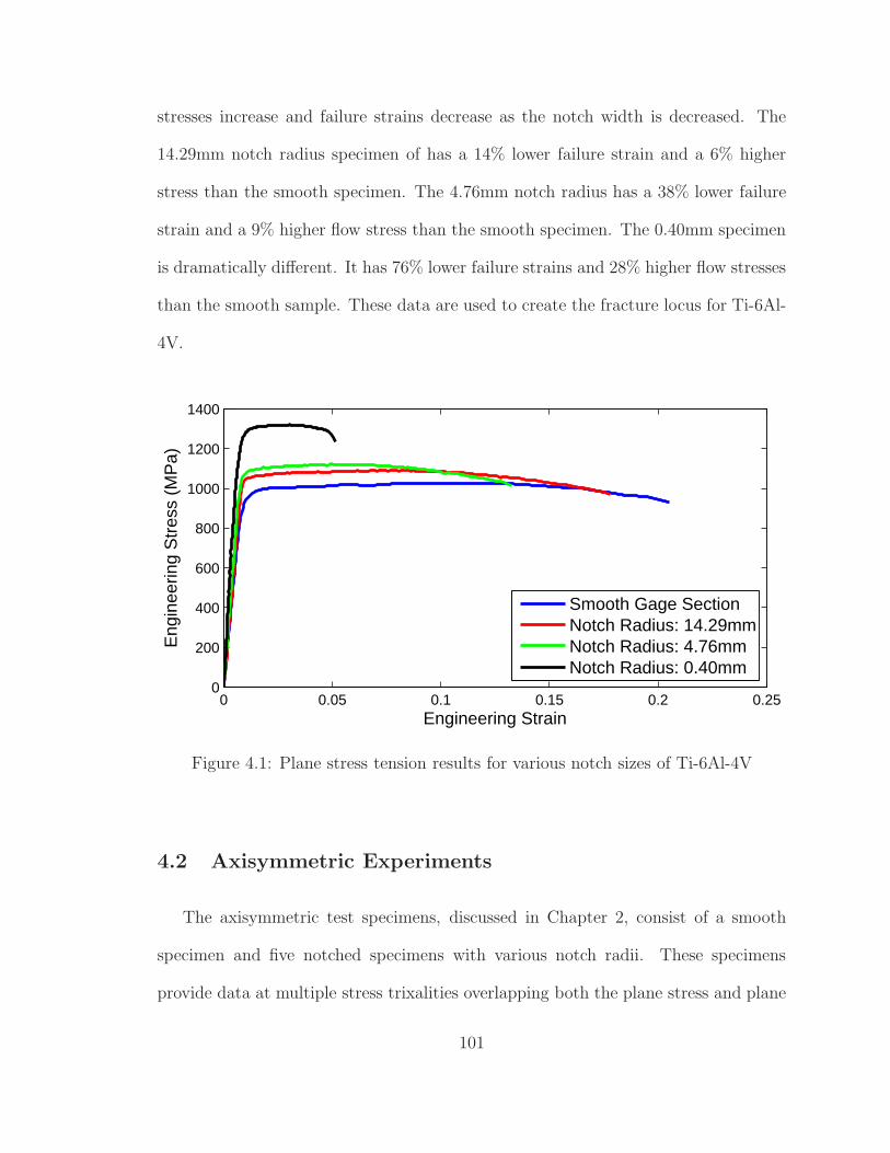
stresses increase and failure strains decrease as the notch width is decreased. The
14.29mm notch radius specimen of has a 14% lower failure strain and a 6% higher
stress than the smooth specimen. The 4.76mm notch radius has a 38% lower failure
strain and a 9% higher flow stress than the smooth specimen. The 0.40mm specimen
is dramatically different. It has 76% lower failure strains and 28% higher flow stresses
than the smooth sample. These data are used to create the fracture locus for Ti-6Al-
4V.
0 0.05 0.1 0.15 0.2 0.250
200
400
600
800
1000
1200
1400
Engineering Strain
Eng
inee
ring
Str
ess
(MP
a)
Smooth Gage SectionNotch Radius: 14.29mmNotch Radius: 4.76mmNotch Radius: 0.40mm
Figure 4.1: Plane stress tension results for various notch sizes of Ti-6Al-4V
4.2 Axisymmetric Experiments
The axisymmetric test specimens, discussed in Chapter 2, consist of a smooth
specimen and five notched specimens with various notch radii. These specimens
provide data at multiple stress trixalities overlapping both the plane stress and plane
101

strain points. Triaxialities range from 0.369 to 0.956. All specimens have a Lode
number equal to one due to their cross sectional geometry.
Axisymmetric test results are presented in Figure 4.2. As previously discussed,
with decreasing notch radii the stresses increase and failure strains decrease. The
axisymmetric smooth specimen has a failure strain of 0.33 and a peak flow stress of
1045MPa. Failure strains decrease by 40%, 42%, 48%, 55%, and 67% while flow
stresses increase at 7%, 11%, 13%, 19%, and 26% from the smooth specimen for the
respective notches. These data are used to formulate the fracture locus.
0 0.05 0.1 0.15 0.2 0.25 0.3 0.350
500
1000
1500
Engineering Strain
Eng
inee
ring
Str
ess
(MP
a)
Smooth Gage SectionNotch Radius: 34.93mmNotch Radius: 17.46mmNotch Radius: 11.91mmNotch Radius: 6.75mmNotch Radius: 3.18mm
Figure 4.2: Axisymmetric tension results for various notch sizes of Ti-6Al-4V
4.3 Plane Strain Experiments
Plane strain specimens, as discussed in Chapter 2, are dog bone specimen with
much larger thickness than width. The large thickness ensures that the transverse
102

compressive strains are approximately zero at the center of the specimen. DIC mea-
surements are used to confirm this assumption.
The test results are presented in Figure 4.3. The three specimens represent stress
triaxialities ranging from 0.470 to 0.768. Again, as notch radius decreases, the stresses
increase and failure strains decrease. The plane strain smooth specimen has an ap-
proximate peak stress of 1092MPa and a failure strain of 0.17. The 12.7mm notch
radius specimen has a 30% lower failure strain and a 7% higher stress than the smooth
sample. The 4.76mm notch radius specimen has a 53% lower failure strain and a 16%
higher stress than the smooth sample.
0 0.02 0.04 0.06 0.08 0.1 0.12 0.14 0.16 0.18 0.20
200
400
600
800
1000
1200
1400
Engineering Strain
Eng
inee
ring
Str
ess
(MP
a)
Smooth Gage SectionNotch Radius: 12.70mmNotch Radius: 4.76mm
Figure 4.3: Plane strain tension results for various notch sizes of Ti-6Al-4V
Strain field, measured with DIC, are seen in Figure 4.4. These strain fields are
just prior to specimen failure. Ideally, the transverse strain (ǫ2) at the center of the
specimen would be zero, which gives a perfect plane strain condition. The data in
103

Figure 4.4 shows that the transverse strain in the center of the specimen is not zero.
The notched specimens have substantially less transverse strains than the smooth
sample. The stress and strain state of the smooth sample is not ideal. This results
in the high Lode parameter value (0.506) for the plane strain smooth specimen.
Figure 4.4: DIC strain field data from plane strain specimens with various geometries
4.4 Combined Loading Experiments
Thin walled tube specimens are loaded in tension-torsion (σ/τ = 1.971 and σ/τ =
0.847), torsion (σ/τ = 0), and compression-torsion (σ/τ = −0.847) to gain additional
fracture locus data points. Data from these tests are presented in Figure 4.5. The
combined loading specimens have stress triaxialities ranging from -0.148 to 0.252 and
lode parameters ranging from -0.394 to 0.706. The displacement and angle of rotation
data presented in Figure 4.5 is acquired from digital image correlation. Displacement
104

of two points, roughly 3mm apart on the surface of the specimen are used to calculate
the displacements and rotations. Displacement is simply the difference in the vertical
motion of the two points. The angle of rotation is calculated using data from these
points in equation 2.5. This is the same method used to determine angle of twist and
shear strain in the torsional experiments described in Chapter 3. Time history of a
tension-torsion experiment is seen in Figure 4.6
As the axial to shear stress ratio increases, the failure angles decrease. The
compression-torsion sample (σ/τ = −0.847) has a larger cross sectional area to
prevent buckling in the specimen during loading. Although these specimens have
a larger wall thickness, they require a similar angle of rotation at failure than its
tension-torsion counterpart (σ/τ = 0.847). Initially, the stress state parameters are
fluctuating they settle at the desired values following yielding of the specimen, see
Figure 4.6. Unlike with the tension tests, the stress states do not evolve significantly
after yielding for the combined loading tests. Stress, strain, and stress state time
histories can be found in Appendix B for each of the loading conditions.
0 0.2 0.4 0.6 0.80
5
10
15
20
Displacement (mm)
Axi
al F
orce
(kN
)
σ/τ=1.971σ/τ=0.847σ/τ=0.00σ/τ=−0.847
0 5 10 150
20
40
60
80
100
Angle (degree)
Tor
que
(Nm
)
Figure 4.5: Combined axial-torsional test results for various notch sizes of Ti-6Al-4V
105

0 10 20 30 40 50 60 70 800
100
200
300
400
500
600
700
800
900
Str
ess
(MP
a)
−0.2
0
0.2
0.4
0.6
0.8
1
1.2
Str
ess
Sta
te P
aram
eter
0 10 20 30 40 50 60 70 80−0.2
−0.15
−0.1
−0.05
0
0.05
0.1
0.15
0.2
0.25
Str
ain
Time(s)
Axial Stress [σyy
]
Shear Stress [σxy
]
Max Principle Strain [ε1]
Min Principle Strain [ε2]
Triaxiality [σ*]
Lode Prameter [µ]
Figure 4.6: Time history of a tension-torsion experiment
4.5 Fracture Point Determination and Locus Creation
For tension tests, fracture locus points and stress states are found by analyzing
test data and parallel simulations, see Figure 4.7. This procedure is introduced in
Subsection 2.3.5. The simulated data is cropped at the drop in load and the physical
tests, which indicates a specimen failure. The DIC frames are shown one frame
prior to failure while the simulation is shown at the equivalent displacement to the
DIC. The curves from both are also shown. The blue curves represent the stress,
the green represent the strain, and the red represent the stress state parameters. A
vertical gray line represents the fracture point. Three variations of strain are shown,
center simulation, surface simulation, and surface DIC. The center simulation and
surface simulation differ slightly due to high stresses and therefore higher strains in
106

the center of the specimen. The two surface strains differ due to differences in gage
lengths between the simulation mesh and the DIC.
These parallel experiments and simulations are completed for each of the phys-
ical tests to asses fracture strain data spread. The stress state is calculated using
Equations 1.4 and 1.8 from simulated stress state records extracted at the internal
element up to the identified point of failure. Combined loading stress states and frac-
ture strains are found from experimental data. Fracture strains are measured using
DIC. Care was taken to ensure that virtual strain gage lengths are similar to those
of the tension specimens. Stress state parameters are calculated from the axial force
and torque data using Equations 2.15 and 2.16. A history plot of the combined load
tension-torsion test can be seen in Figure 4.6. Results for each of these tests can be
seen in Table 4.1. Comparison of simulated and experimental data for each tension
geometry can be seen in Appendix D.
Failure strain data is plotted versus stress triaxiality and Lode parameter in Fig-
ure 4.8. In these plots, plane stress specimens are represented with blue squares,
the axisymmetric specimens with red circles, the plane strain specimens with green
triangles, and the combined loading specimens with black diamonds. Error bars rep-
resent the range of failure strain for each load condition. The plane stress smooth
specimens and the axisymmetric smooth specimens have the largest ranges of fail-
ure strains. Some specimens have similar stress states yet large differences in failure
strains. For example, the SG11, SG6, and SG3 specimens have similar triaxialities
(σ∗ ≈ 0.484) but failure strains ranging from 0.20 to 0.46. The LR3, SG12, SG13,
and SG4 tests all have similar Lode parameters (µ ≈ 0.016) but failure strain range
from 0.12 to 0.49. Neither of these stress state parameters can accurately describe the
107

Figure 4.7: Data from an experiment and parallel simulation of a plane stress speci-men
108

Table 4.1: Results of the ductile fracture of Ti-6Al-4V testingTest Geometry
GeometryFailure Stress Lode
No. Type Strain Triaxiality Parameter
SG1 0.59 0.400 0.845
SG2 0.44 0.431 0.719Plane
SG3Stress
0.43 0.489 0.528
SG4 0.14 0.583 0.014
SG5
Axisymmetric
0.31 0.369 1.0
SG6 0.31 0.492 1.0
SG7 0.32 0.564 1.0
SG8 0.27 0.618 1.0
SG9 0.27 0.751 1.0
SG10 0.22 0.956 1.0
SG11 0.21 0.470 0.506
SG12Plane
0.22 0.660 0.040Strain
SG13 0.21 0.768 0.025
LR1 0.29 0.252 0.706
LR2 0.51 0.150 0.400Combined
LR3Loading
0.43 0.00 0.00
LR4 0.42 -0.148 -0.394
109

failure behavior of Ti-6Al-4V individually. Together, however, a three dimensional
fracture locus can be defined using both triaxiality and Lode parameter.
−0.2 0 0.2 0.4 0.6 0.8 10
0.1
0.2
0.3
0.4
0.5
0.6
0.7
0.8(a)
Stress Triaxiality
Fal
iure
Str
ain
−0.5 0 0.5 10
0.1
0.2
0.3
0.4
0.5
0.6
0.7
0.8(b)
Lode Parameter
Plane StressAxisymmetricPlane StrainCombined Loading
Figure 4.8: Failure strain versus triaxiality(a) and Lode parameters(b) for each of thespecimen geometries and loading conditions
The Ti-6Al-4V fracture surface is presented in Figure 4.9. Equivalent plastic fail-
ure strain is plotted on the z-axis versus stress triaxiality and Lode parameter on the
x-axis and y-axis, respectively. Plane stress, plane strain, and combined loading re-
sults are represented by circles, triangles, and diamonds, respectively. Axisymmetric
specimens are displayed as square markers (Lode parameters equal to one). Bihar-
monic Spline Interpolation[34] is used to create the surface. Areas of low strain are
represented in blue while high strains are represented in red. A low valley transitions
into a high peak because the plane strain (SG11) and plane stress (SG3) data. These
two specimens have considerably different geometries and fracture strains yet similar
stress state parameters. It is possible that triaxiality and Lode parameter are not
110

enough to characterize the fracture surface of Ti-6Al-4V. It is also possible that fail-
ure does not occur exactly at the centers of the samples, as have been assumed here.
Further study on the subject my be warranted.
Figure 4.9: Three dimensional view of the Ti-6Al-4V fracture locus
4.6 Johnson-Cook Fracture Parameter Determination
Johnson-Cook fracture parameters are determined from the test data presented in
this Chapter as well as Chapter 3. Fracture strain data at several stress triaxialities,
temperatures, and strain rates is required to formulate these parameters. Failure
strains used to determine the stress state dependence parameters (D1, D2, and D3)
are those found in the previous section. Failure strains used to determine the strain
rate dependent parameter (D4) are measured with 4mm DIC extensometers described
in the plastic deformation testing. Failure strains used to determine the temperature
dependent parameter (D5) are measured with a 2mm DIC extensometer. A smaller
111

extensometer is to capture the increased localization strains as temperature increases.
Data at various temperatures and strain rates, previously shown in Chapter 3, are
assumed to have a stress triaxiality of 0.400. Strain data from extensometers are used
to determine the parameters instead of parallel simulations.
Parameters from each bracketed expression in Equation 1.2 are found individually.
The various stress state tests are performed at a strain rate of 1.0×10⁻²s−1. Since
the reference strain rate (ǫo) is 1.0s−1, the strains used to find these parameters will
he higher than if the tests were performed at the reference strain rate. A scale factor
is used to adjust D1 and D2 which is found from D4 and is given by
SF =
[
1 +D4 ln
(
1.0× 10⁻²s−1
1.0s−1
)]
−1
. (4.1)
Parameters D1, D2, and D3, are fitted to data at various stress states (Figure 4.10)
at the test strain rate (ǫo = 1.0 × 10⁻²s−1) and temperature (T = 25C). At the
reference strain rate and temperature the JC fracture equation is
ǫpf =[
D1 +D2eD3σ
∗]
. (4.2)
Figure 4.10 shows the model predicted fracture strain. D1, D2, are determined and
scaled to be −0.81 and 1.18, respectively. D3 is determined to be −0.15. Compared to
the experimental data the newly determined parameters predict significantly higher
strains than the parameters previously determined by Johnson[22]. Clearly, Johnson’s
parameters underestimate all of the fracture strain data in Figure 4.10. As discussed
in Section 4.5, some of these specimens have similar stress triaxialities yet considerably
different fracture strains. This indicates a short coming in The Johnson-Cook fracture
model, which defines the failure strain as a function of only the stress triaxiality.
Therefore it is unable to capture the fracture strain spread plotted in Figure 4.10.
112

−0.2 0 0.2 0.4 0.6 0.8 10
0.1
0.2
0.3
0.4
0.5
0.6
0.7
0.8
Stress Triaxiality
Fal
iure
Str
ain
Plane StressAxisymmetricPlane StrainCombined LoadingHammer ParametersJohnson Parameters
Figure 4.10: Johnson-Cook fracture strain predictions compared to experimentaldata: stress state sensitivity
The term, D4, is found by curve fitting normalized fracture strain data at different
strain rates. The normalized fracture strain is
ǫpfǫr
=
[
1 +D4 ln
(
ǫ
ǫo
)]
, (4.3)
where,
ǫr =[
D1 +D2eD3σ
∗]
[
1 +D5
(
T − Tr
Tm − Tr
)]
, (4.4)
where, σ∗ is equal to 0.400 and T = 25C. Normalized fracture strain data are plotted
with the best fit in Figure 4.11. From this fit the D4 term is found to be −0.012.
The data shows that fracture strain decreases slightly with increasing strain rate.
Johnson’s parameters underestimate the fracture strains and predict that fracture
strain increases with strain rate.
113

10−5
10−3
10−1
101
103
105
0
0.05
0.1
0.15
0.2
0.25
Strain Rate (s−1)
Nor
mal
ized
Fra
ctur
e S
trai
n
P4 Tension DataJohnson ParametersHammer Parameters
Figure 4.11: Johnson-Cook fracture strain predictions compared to experimentaldata: Strain rate sensitivity
The final JC parameter, D5, is determined by curve fitting normalized fracture
strain data at various temperatures. The normalized fracture strain is
ǫpfǫr
=
[
1 +D5
(
T − Tr
Tm − Tr
)]
, (4.5)
where,
ǫr =[
D1 +D2eD3σ
∗]
[
1 +D4 ln
(
ǫ
ǫo
)]
, (4.6)
where, σ∗ is equal to 0.400 and ǫ/ǫo is equal to one. A D5 parameter value of 2.10 is
determined to best fit the data. Normalized fracture strain data are plotted with the
best fit prediction in Figure 4.12. The Johnson parameters overestimate the fracture
strain of this material.
114

0 0.05 0.1 0.15 0.2 0.25 0.3 0.35 0.4 0.45 0.50.5
1
1.5
2
2.5
3
T*
Nor
mal
ized
Fai
lure
Str
ain
Fracture PointsJohnson ParametersHammer Parameters
Figure 4.12: Johnson-Cook fracture temperature parameter determination
Chapter 3 shows large differences in not only flow stress but also failure strains
between various plate stocks. This explains why the Johnson parameters do a rela-
tively poor job of predicting the fracture behavior of the 12.7mm thick plate describe
here. It is important to fully characterize the response of the working material prior
to using Johnson-Cool Material parameters found in the literature. Figure 4.10 shows
that it is advantageous to use more complex models, such as MAT224, since stress
triaxiality alone is unable to describe this material’s failure properties.
4.7 Conclusions for the Ti-6Al-4V Fracture Testing
The ductile fracture of Ti-6Al-4V at several stress triaxialities and Lode param-
eters is experimentally tested. The testing is completed on plane strain (thin, flat),
axisymmetric (round cross sectional), plane strain (thick, flat), and combined loading
115

(thin walled tube) specimens. For each of the tension specimens, several geometries
are tested with increasingly sharp notches. With decreasing notch radius, fracture
strains decrease and stresses increase. Increasing temperatures gives higher failure
strains due to an increase in ductility. Failure strain decreases slightly with increas-
ing strain rates. As seen in Chapter 3 the material can also have different failure
strains in different orientations.
As seen in Figure 4.8, the stress triaxiality is clearly not enough to fully character-
ize the failure of the material. The Lode Parameter is included for a more complete
description of the stress state at failure. From these data a fracture locus has been
created, additional views of which are available in Appendix E.
New Johnson-Cook fracture model parameters are determined and presented in
Table 4.2. There are substantial differences than those determined by Johnson[22].
The differences between the two sets of fracture model parameters are most likely
caused by differences in plate stocks. Care should be taken to ensure that the model
parameters adequately capture the failure behavior of the specific plate stock.
Table 4.2: Comparison of Ti-6Al-4V Johnson-Cook constitutive parameters found inthe literature to those determined for plate 4
Name A(MPa) B(MPa) n C m D1 D2 D3 D4 D5
Johnson 862 331 0.34 0.012 0.8 −0.09 0.25 −0.5 0.014 3.87
Lesuer 1098 1092 0.93 0.014 1.1 – – – – –
Yatnalkar 1055 426 0.50 0.023 0.8 – – – – –
Milani 1051 924 0.52 0.0025 0.98 – – – – –
Hammer 1062 431 0.50 0.016 0.69 −0.81 1.18 −0.15 −0.012 2.10
116

Chapter 5: Summary and Conclusions of the Ti-6Al-4V
Testing
Plastic deformation and ductile fracture of Ti64 is investigated experimentally.
Plastic deformation behavior is presented in Chapter 3 while the ductile fracture
behavior is presented in Chapter 4. Plastic deformation characterization is performed
for four different plates with thicknesses of 2.29mm, 3.56mm, 6.35mm, and 12.7mm.
These plates are labeled Plate 1, 2, 3, and 4, respectively. The ductile fracture testing
is performed only on Plate 4. The testing was funded by the FAA’s Uncontained
Engine Debris Mitigation Program, the ultimate goal of which is to make jet engines
more reliable and safer to operate. Differences discussed in the materials are outside
of data spread, which can be seen in Appendix A and B. These data are used by
GWU and the FAA to calibrate the LS-DYNA material model, MAT224.
5.1 Plastic Deformation Experimental Conclusions
Detailed results from the plastic deformation test series are found in Chapter
3. Experimental methods used to determine the plastic deformation characteristics
are described, at length, in Chapter 2. Limited tension and compression tests are
conducted on plates 1 and 2 while plates 3 and 4 are subject to a comprehensive test
plan. Plate 4 also includes shear testing. The majority of the plate 3 testing was done
117

by Yatnalkar[12]. A complete test outline is presented in Table 2.1. Tension testing is
conduced with similarly sized plane stress smooth dog-bone specimens. Compression
testing is completed with cylinder specimens. Torsion tests are conducted on thin
walled tube specimens. Load measurements are taken using either a load cell or
Kolsky bar depending on the test setup and strain rate. Displacements and strains
are measured with three dimensional digital image correlation.
Strain rate dependent testing is conducted in tension and torsion at strain rates
between 1.0× 10⁻⁴s−1 and 1.5× 10³s−1 and in compression up to 8.0× 10³s−1. The
material displays significant rate dependence throughout the entire range of strain
rates. The material has increasing yield and flow stresses with increasing strain rate.
Plates 3 and 4 show a significant change in strain hardening rate between 1.0×10⁻²s−1
and 1.0s−1 in both tension and compression. Failure strain is also influenced by the
strain rate where lower failure strains are measured at high strain rates. Shear test
results for plate 4 show similar trends in shear stresses and failure strains for increasing
strain rates.
Anisotropic properties within the plate are investigated by testing specimens ma-
chined in the rolled, 45 from rolled, transverse, and −45 from rolled directions.
Compression anisotropic testing is also conducted in the through direction. In ten-
sion, plates 1, 3, and 4 display an anisotropic behavior while plate 2 is isotropic for
the directions tested. In compression, plate 3 has significant anisotropic behavior
while plate 4 appears only slightly anisotropic. Depending on the plate stock, differ-
ences are seen in yield stress, flow stress, strain hardening rates, and failure strain
in both tension and compression. There is also asymmetry between the tension and
compression characteristics.
118

For plates 3 and 4 tests are performed at various temperatures ranging from−50C
to 600C. Results from these tests indicate that yield and flow stress, strain hardening,
failure strains, and failure mode are strongly dependent on temperature. Flow stresses
decrease and failure strain increase as temperatures increase. At low temperatures,
compression specimens exhibit shear failure while at higher temperatures they do not.
The two plates have converging material responses at 200C in tension and at 600C
in compression.
Although each of the four plate stocks fall under the same AMS specification,
a comparison between them shows significant differences in the material properties.
These differences are seen in the yield and flow stresses, strain hardening, failure
strains, and failure modes. The strength of Plate 4 is higher than the others. Plate 3
has the highest degree of anisotropy while plate 2 is essentially isotropic. Anisotropic
effects are also not similar between the plates. All plates showed tension/compression
asymmetry.
5.2 Ductile Fracture Experimental Conclusions
Detailed results from the ductile fracture test series are found in Chapter 4. Meth-
ods used to test the fracture specimens are described, in detail, in Chapter 2. All
specimens in this test series are fabricated from Plate 4 in the rolled direction. Com-
plete testing outlines are presented in Tables 2.2, 2.4, 2.3, and 2.5. Experimental
data are compared to simulation results in Appendix D. Ductile fracture tests are
conducted on plane stress, axisymmetric, and plane strain tension specimens and com-
bined loading (thin-walled tube) specimens. Four different plane stress specimens are
tested, including: a smooth dog-bone and three notched specimens. Axisymmetric
119
specimens include: one smooth and five with various sized notches. Plane strain
specimens include: one smooth and two notched specimens. Combined loading tests
include four different axial-torsional loading rations. Force and torque are measured
with a load cell and displacements are measured with three dimensional digital image
correlation.
As the notch radius decreases for plane stress, axisymmetric, and plane strain
specimens the stresses increases and the failure strain decreases. Plane stress speci-
mens have stress triaxialities ranging from 0.400 to 0.583, Lode parameters ranging
from 0.014 to 0.845, and failure strains from 0.14 to 0.59. Axisymmetric specimens
have stress triaxialities ranging from 0.369 to 0.956, Lode parameters all equal to 1.0,
and failure strains from 0.22 to 0.31. Plane strain specimens have stress triaxialities
ranging from 0.470 to 0.768, Lode parameters from 0.025 to 0.506, and failure strains
from 0.21 to 0.22. Combined loading specimens have stress triaxialities ranging from
−0.147 to 0.251, Lode parameters ranging from −0.390 to 0.702, and failure strains
from 0.29 to 0.51. Models that use the stress triaxiality alone to describe failure strain
are unable to predict the failure of the specimen under the various loading conditions
tested. The Lode parameter is used to create a three dimensional fracture locus in
the stress triaxiality and Lode parameter stress space.
Failure strains found by comparing experimental data to simulation results are
used to construct the locus. These strains are determined from the center element of
the simulated specimen since theory indicates failure will initiate there[28]. Multiple
views of the fracture locus are found in Appendix E. The fracture locus can be used
to predict fracture of Ti-6Al-4V under various states of stress. These data are used
to calibrate the MAT224 fracture model for Ti-6Al-4V.
120
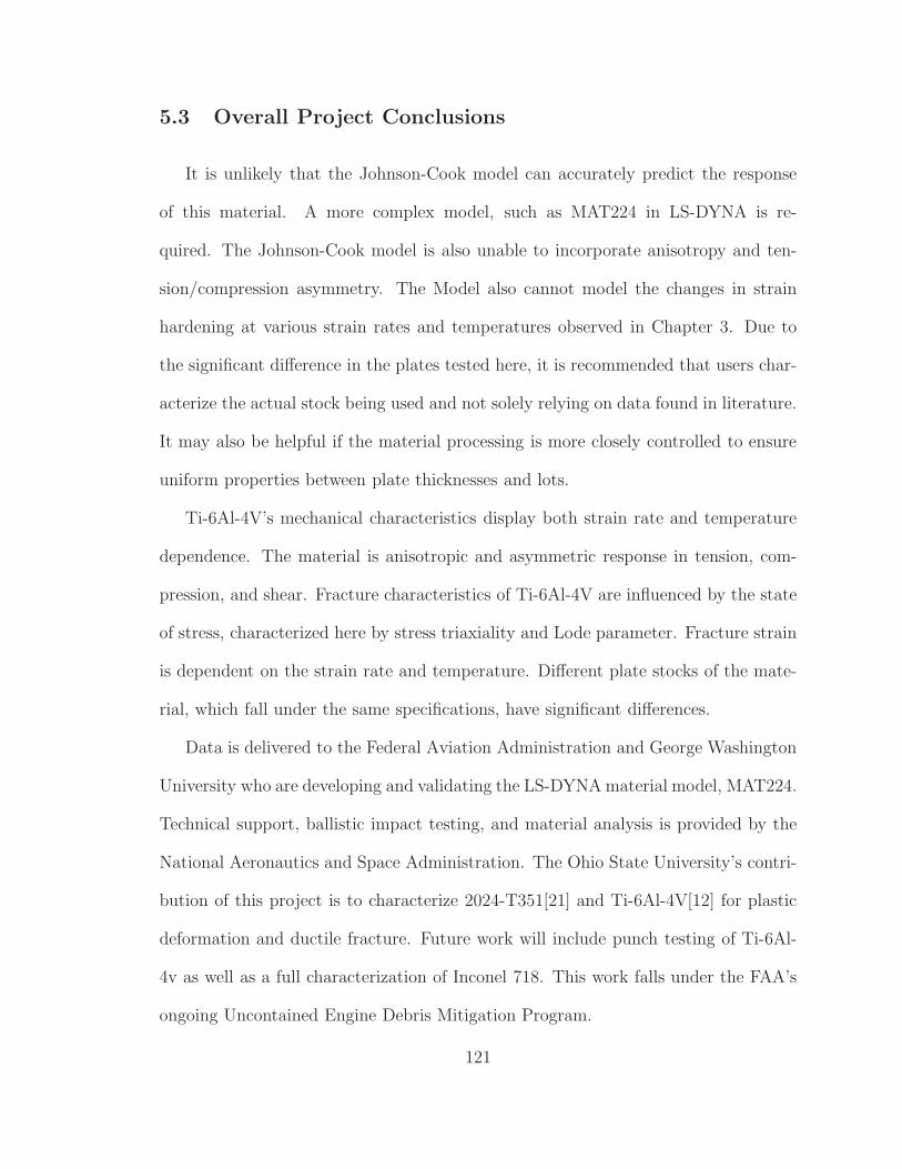
5.3 Overall Project Conclusions
It is unlikely that the Johnson-Cook model can accurately predict the response
of this material. A more complex model, such as MAT224 in LS-DYNA is re-
quired. The Johnson-Cook model is also unable to incorporate anisotropy and ten-
sion/compression asymmetry. The Model also cannot model the changes in strain
hardening at various strain rates and temperatures observed in Chapter 3. Due to
the significant difference in the plates tested here, it is recommended that users char-
acterize the actual stock being used and not solely relying on data found in literature.
It may also be helpful if the material processing is more closely controlled to ensure
uniform properties between plate thicknesses and lots.
Ti-6Al-4V’s mechanical characteristics display both strain rate and temperature
dependence. The material is anisotropic and asymmetric response in tension, com-
pression, and shear. Fracture characteristics of Ti-6Al-4V are influenced by the state
of stress, characterized here by stress triaxiality and Lode parameter. Fracture strain
is dependent on the strain rate and temperature. Different plate stocks of the mate-
rial, which fall under the same specifications, have significant differences.
Data is delivered to the Federal Aviation Administration and George Washington
University who are developing and validating the LS-DYNAmaterial model, MAT224.
Technical support, ballistic impact testing, and material analysis is provided by the
National Aeronautics and Space Administration. The Ohio State University’s contri-
bution of this project is to characterize 2024-T351[21] and Ti-6Al-4V[12] for plastic
deformation and ductile fracture. Future work will include punch testing of Ti-6Al-
4v as well as a full characterization of Inconel 718. This work falls under the FAA’s
ongoing Uncontained Engine Debris Mitigation Program.
121

Chapter 6: Strain Measurements at Temperatures up to
800C utilizing Digital Image Correlation
6.1 Introduction
Measuring strain at elevated temperatures is challenging. This chapter presents
a straight forward and repeatable method to measure full field strains at tempera-
tures up to 800C using a three dimensional Digital Image Correlation system. High
temperature strain measurement techniques include: 1)using the signal from the con-
troller LVDT, 2)high temperature extensometer, and 3)high temperature strain gages.
The LVDT is subject to machine compliance errors that vary from test to test with
parameters such as grip location, grip force, or push/pull rod material and length.
High temperature extensometers measure the strain between two ceramic knife edges
attached to the specimen. The actual body of the extensometer typically sits outside
the heated zone and can be water cooled. These extensometer work well but they
assume that the strain is uniform between the knife edges, often have a limited strain
measuring range, and need to be removed prior to specimen failure. High temperature
strain gages can be cumbersome to use. These gages need to be temperature com-
pensated since their gage factors change with temperature. They often have a limited
strain measurement range and they only give data at one point on the specimen.
122

The goal of this chapter is to develop a method to optically measure strain at ele-
vated temperatures up to 800C. Results from this method do not exceed a reasonable
DIC projection errors as compared to room temperature measurements. Thermal ex-
pansion tests are performed with the technique and are used to validate the test
method by comparing to measured CTE’s handbook values. DIC greatly enhances
data because transverse, shear strains, and out of plane displacements can be mea-
sured on the entire visible surface of the specimen. These measurements are very
useful to study both the plastic deformation and failure behavior of materials at
elevated temperatures.
Using DIC above room temperatures has significant challenges. First, the sam-
ple must be visible to external cameras, effectively ruling out close-box furnaces and
induction. Thermal lensing of gases (air) can cause optical problems for the mea-
surement system. If a furnace with a window is used, the window must be free to
expand. If it is confined, it may deform and create a lensing effect. Survivability of
the speckle pattern is also an issue. Standard paints cannot survive elevated temper-
atures making them impractical for this application. The paint must endure the high
temperatures and the larger deformations caused by typical increases in ductility at
these temperatures.
6.1.1 Literature Review
Digital Image Correlation has become an invaluable tool in experimental mechan-
ics and researchers are adapting this measurement technology for use at, more com-
plex, test conditions. Previous researchers have used DIC at elevated temperatures
including: Lyons et al.[35], Grant et al.[36] and Pan et al.[37]. These researchers use
123

various methods and equipment and their work provides valuable insight for those
using DIC at elevated temperatures.
Lyons[35] evaluates a method using a furnace to heat a specimen while collecting
image data through a window at temperatures up to 650C. The furnace window
and variations in the refractive index of the heated air were found to be sources
of error in the measurement. A sapphire window was used and the accuracy of
the measured displacement field was strongly influenced by its optical quality. The
addition of an external fan and optical grade sapphire window reduced these errors to
acceptable levels. Coefficient of Thermal Expansion (CTE) and elastic deformation
measurements were taken.
Grant[36] investigates the use of DIC in measuring CTE at temperatures up to
800C using CCD camera sensors. The researchers found that infrared radiation (IR)
had a negative effect on the measurements. They developed a technique using blue
illuminators and optical bandpass filters to reduce these effects. These illuminators
and filters allowed only light at the upper range of the visible spectrum (420nm to
480nm) through to the CCD, thus reducing detrimental IR.
Pan, et al.[37], demonstrate a method using DIC to measure full field deformations
at temperatures up to 1200C using CMOS camera sensors. The researchers had
similar problems with IR effects and were able to minimize them with the use of a
bandpass filter (428nm to 470nm) and blue light illumination. A black speckle pattern
was applied to the bare metal. The pattern was made from black cobalt oxide mixed
with a commercial high temperature inorganic adhesive. Specimens were heated using
an infrared radiator and CTE were measured.
124

6.2 Experimental Setup
The method introduced here uses a custom enclosed furnace which uniformly
heats the specimen. This furnace was designed in conjunction with Applied Test
Systems Inc. The digital image correlation system needs to be calibrated prior to
testing. The calibration could be rendered invalid by positionary changes between
the cameras and the specimen. Vic-3D defines a three dimensional world coordinate
system from two dimensional images of a grid with known spacing in both camera
sensors. Changes in the optical path for the stereo rig to the specimen will increase the
measurement error. To maintain a consistent optical path, the front of the furnace,
which contains the window, is rigidly mounted to the load frame. The back of the
furnace opens on a hinge granting access to the specimen, see Figure 6.1(c). The
38.1mm×101.6mm window is made from optical quartz, see in Figure 6.1(a). Since the
back section of the furnace opens, the calibration can be preformed without significant
window displacements. Optical quartz combines good thermal properties with low
light deflection reducing lensing, which can cause errors in DIC measurements. The
window is mounted in a ceramic fixture that allows it to freely expand minimizing
internal stresses that may cause lensing.
The furnace includes an internal Inconel 718 fan to circulate the air which is
powered by an external motor mounted on top. The air circulation allows for faster
and more uniform specimen heating. The circulation also reduces thermal lensing
from optical distortions that are caused by temperature gradients in the air that
change the local refractive index. The fan is connected to the motor through an
external chain drive and rotates at 40rpm.
125

(a) (b)
(c)
Figure 6.1: Furnace used with digital image correlation, (a)optical quartz window,(b)3D DIC system setup, (c)interior of furnace
126

Photron MC2.1 cameras are mounted vertically due to the orientation of the win-
dow as seen in Figure 6.1(b). The cameras are operated at 512 × 512 resolution at
1000fps. Sigma 50mm F2.8 DG Macro lenses provided a suitable field of view for the
specimens. CMOS camera sensors are known to be susceptible to IR light[35] and
thus filters are used to increase image quality. Two types of IR filters are generally
available. These are absorptive filters and a reflective filters. The former reduces IR
by absorbing the energy, possibly causing the filters to heat up and thermally expand.
Filter deformation is a concern since this could have a lensing effect and give higher
correlation errors. The latter filter type reflects the light, reducing temperature in-
creases due to IR heating. Tiffen Hot Mirror reflective IR filters are used to prevent
heating and deformation of the filter. The hot mirror filter reduces IR pollution
by reflecting wavelengths above 700nm as seen in Figure 6.2[38]. Fiber optic lamps
provide the necessary lighting through the window as seen in Figure 6.1(b). Image
glare is removed using B+W 55mm linear polarization filters. The polarization filters
are placed between the lenses and the hot mirror filter to reduce the effects of heat-
ing. The recorded images provide sufficient contrast for the digital image correlation
software.
Force and torque are measured using an axial-torsional load cell mounted in series
with the upper grip. A heat shield between the furnace and the load cell prevents
temperature increases in the cell from convection and radiation. To prevent conduc-
tion heat transfer, the grips are water cooled outside of the furnace which keeps the
grip temperature near the load cell at or below room temperature. The furnace has
two thermocouples that provide feedback for a PID controller. The surface of the
specimen is instrumented with at least one attached thermocouple using Omega CC
127

Figure 6.2: Wavelengths of transmitted electromagnetic radiation through Tiffen hotmirror lenses
high temperature cement. The grips were also measured with thermocouples. When
more than one thermocouple was attached to the specimen, the average between
the two at the time of test was recorded as the test temperature. During heating,
temperature data is logged at a rate of 1Hz and saved for further analysis.
Normal paint is not a viable option at these temperatures. Materials typically be-
come more ductile the closer they get to their melt temperatures, so larger strains are
expected in localization regions. This requires flexible paint to deform with the spec-
imen without delaminating. The previous work discussed in Section 6.1.1 considered
elastic deformation or small displacements due to thermal expansions [35][36][37]. For
Ti-6Al-4V, local plastic strains on the order of 50% to 60% are expected at 600C.
Commercially available Rust-oleum High Heat paint, which has a reported operating
temperature of 1093C is used for the base coat and speckel pattern.
128

6.3 Validation of Measurement System
6.3.1 Optical Validation
Figure 6.3 shows the optical quality of digital pictures taken with the cameras,
lenses, filters, and paint described above. These pictures show the evolution of the
image quality as the temperature increases up to 900C. The images get darker as
temperature is increased to 700C. The increase in light above this temperature is
due to significant IR emanating from the Inconel Bars. The image quality is generally
good and has enough contrast to calculate DIC data up to 800C.
Figure 6.3: Image quality from room temperature to 900C
6.3.2 Coefficient of Thermal Expansion Validation Testing
The introduction of a new measurement method requires initial validation testing.
To validate the experimental setup, images of a test specimen are recorded as temper-
ature is increased. Temperature is increased in steps to allow the system to stabilize.
129

Three dimensional digital image correlation is used to measure the increase in length
as the material expands due to the increase in temperature. From the measured
displacements, the coefficient of thermal expansion, α, is calculated through:
α =Li (Tf − Ti)
∆L, (6.1)
where ∆L, is the change in specimen length, Li is the initial measured length, and
Tf and Ti are the final and initial temperature, respectively. Ti-6Al-4V is tested
because it has been extensively studied and tabulated [39]. Measured CTE’s at various
temperature differences, ∆T , are plotted with published data in Figure 6.4[39]. The
data shows good correlation at ∆T ’s above 450C. Displacement measurements at
lower temperatures were susceptible to noise due to the small deformations.
300 400 500 600 700 800 9007
8
9
10
11
12
Change in Temperature [∆T] (oC)
CT
E [α
] (µm
/m/o C
)
Measured ValueReference Value
Figure 6.4: Comparison of measured Ti-6Al-4V thermal expansion coefficients topreviously published data
130

The validation tests showed good agreement at temperature differences above
450C corresponding to approximately 4500µǫ. The noise to data ratio seen in the
CTE tests are much higher than those in the plastic deformation testing, due to the
much higher strain magnitudes expected. Results from a typical CTE test can be
seen in Figure 6.5[39]. The high levels of noise at the beginning of the test are due
to the small deformations measured with the DIC system. These data coupled with
the low ∆T cause the noise.
0 500 1000 1500 2000 2500 3000 3500−50
0
50
100
150
200
Cha
nge
in L
engt
h (µ
m)
3
4
5
6
7
8
9
10
CT
E (
µm
/m/o C
)
0 500 1000 1500 2000 2500 3000 35000
200
400
600
800
1000
Cha
nge
in T
empe
ratu
re (o C
)Time(s)
Figure 6.5: Measured data from a coefficient of thermal expansion test on Ti-6Al-4V
For each set of images processed Vic-3D quantifies the amount of error and tabu-
lates it. Based on the calibration, a given point in the camera one image has a pre-
dicted line (epipolar line) along which the point must lie in the camera two image[38].
The projection error is the distance, in pixels, from the expected distance and values
below 0.05 are ideal. Projection errors from a CTE test are shown in Figure 6.6. The
131

projection error increases from 0.06 at room temperature to approximately 0.12 at
100C to 860C. Room temperature projection errors are slightly higher then normal
due to the presence of the window. As temperature increases, the projection errors
increase.
0 100 200 300 400 500 600 700 800 9000
0.05
0.1
0.15
0.2
Temperature (oC)
Pro
ject
ion
Err
or
Figure 6.6: Projection error versus temperature for a coefficient of thermal expansiontest on Ti-6Al-4V
The goal of any experimental measurement system is minimize error between the
physical event and the recorded data. There is significant room for errors due to the
complex nature of these tests. Window lensing, gaseous lensing, thermal expansion,
and relative motion of lenses or windows are all potential sources of errors. Although
DIC measurement projection errors are higher at high temperatures they are still
within reasonable levels compared to room temperature tests.
132

6.4 Experimental Methods and Results of the Various Load-
ing Conditions at High-temperatures
High temperature data is required for tension, compression, and torsion (shear).
Techniques for each of the loading types are discussed here. Complete experimental
data can be seen in Chapter 3. Data spread for this data can be seen in Appendix
A. Although, this system is capable of measurements up to 860C tests are only
performed at 200C, 400C, and 600C.
6.4.1 Tension Measurement Techniques and Results
The water cooled Inco718 push/pull rods are aligned using dual depth gages prior
to testing. The grips are specially designed for high temperature tension tests are
seen in Figure 6.7. Both the top and bottom grips have recessed notches with a
similar width to that of the specimen grip section. This recess ensures that each
specimen is properly aligned. The specimen is affixed to the grip with an Inco718
clamp using high temperature #4 − 40 × 1/2 screws. For temperatures at or below
400C a high nickel ferrous alloy (A286) is used, for tests above 400C Inco718 screws
are used. HCP Boron Nitride Powder, a high temperature solid lubricant, is applied
to the threads prior to testing to prevent oxidation and binding of the screws. Two
thermocouples were placed on the bars and two were placed on the specimen just
outside of the gage section using Omega CC high temperature cement.
Digital image quality, at room temperature, 200C, 400C, and 600C, are shown
in Figure 6.8. A 4mm virtual extensometer(see Figure 6.9 at 25C), which sufficiently
spans the gage section, is used to measure strain.
133

Figure 6.7: Grip method and experimental setup for high temperature tension testing
Figure 6.8: Digital image quality of tension specimens at various temperatures
134

DIC results from the tension tests on Ti-6Al-4V at various temperatures are pre-
sented in Figure 6.9. These strain fields correspond to the point just prior to specimen
failure. At elevated temperatures, the paint delaminated resulting in data loss in the
necking region. The 4mm extensometer, however, gave good results at all tempera-
tures. The figure shows that the extensometer is outside of the affected region and
the data is usable until fracture.
Figure 6.9: Axial strain measured with 3D digital image correlation just prior tofailure at various temperatures and speckle pattern adhesion for tension
An engineering stress strain curve constructed using strain data from the 4mm
extenometer is compared to the one constructed using strain from the LVDT is shown
in Figure 6.10. This plot presents data for a tension specimen at 600C at a strain rate
135

of 1.0s−1. The DIC data shows increased stiffness in the initial portion of the curve
and much larger strains after necking begins. The initial deviation between the two
curves is caused by load frame and grip compliance. Since the DIC strain is measured
directly on the surface of the sample, the compliance is eliminated. The post necking
portion of the curve, where DIC strains exceed LDVT strains, can be explained by the
extreme necking localization in the gage section shown in Figure 6.9 at 600C. The
4mm extensometer is close to this localization region. At the onset of necking, the
deformation rate (measured by the extenometer) increases dramatically. The LVDT
strain measurement assumes that all the deformation takes place uniformly within
the 5.08mm smooth section of the sample. This artificially decreases the strain and
creates the variance shown in Figure 6.10.
0 0.05 0.1 0.15 0.2 0.25 0.30
100
200
300
400
500
600
Engineering Strain
Eng
inee
ring
Str
ess
(MP
a)
DICLVDT
Figure 6.10: Comparisons of strain measurements for tension at 600C
136

The reliability of paint adhesion decreased with increasing temperature, see Fig-
ure 6.9. The paint becomes brittle at high temperatures. In addition, Ti-6Al-4V
undergoes larger deformations in the necking region as the material gets closer to the
melting temperature. Strains for the elevated temperature tests are calculated from
a 4mm extensometer which lies outside of the paint delamination region. Alternative
painting options were not explored since the extensometer obtained valuable data. A
new painting method or material is needed to measure failure stains in the localized
region.
6.4.2 Compression Measurement Techniques and Results
Larger compliance errors exits in compression due to the high forces involved.
Compression strains are typically corrected by subtracting the system compliance
from the LVDT record. The system compliance must be determined at each of the
different temperatures. Three dimensional DIC eliminates the need to determine
compliance since measurements are made directly on the compression specimen.
Aligned Inconel 718 push rods are with 12.7mm diameter WC inserts as seen in
Figure 6.11. The specimen is centered on the platens prior to testing. HCP Boron
Nitride Powder is placed between the specimen and the WC inserts to reduce contact
force friction. A compressive, uniaxial loading condition is desired and friction causes
radial stresses. Thermocouples were located on the top and bottom tungsten carbide
platens. Attaching the thermocouple directly to the specimen may artificially increase
the measured load since the Omega CC cement is capable of carrying load.
Ideally, the cameras would be positioned horizontal to the loading direction, but
the orientation of the window makes this impossible. The cameras are carefully placed
137

Figure 6.11: Loading method and experimental setup for high temperature compres-sion testing
vertically so that data is measured both on the specimen and the WC platens. Images
of the platens and compression specimen at 200C, 400C, and 600C are shown in
Figure 6.12. A virtual extensometer, roughly the length of the specimen, is used to
measure elastic strains. The motion of the platens is used to measure plastic strains.
Figure 6.12: Digital images of compression specimens at various temperatures
138

Paint adhesion is also an issue in the compression testing, see Figure 6.13. The
paint delaminated after yield at temperatures at and above 400C. For these tests,
the relative platen motion is used to measure strain. Note that DIC measurements
capture the shear failure mode at 25C and 200C. Ti-6Al-4V is much more ductile
at 400C and 600C as seen in Figure 6.13.
Figure 6.13: Axial strain measured with 3D digital image correlation just prior tofailure at various temperatures and speckle pattern adhesion for compression
Stress strain curves constructed for strains measured with DIC and strains mea-
sured with the LVDT are seen in Figure 6.14. The figure shows data from a com-
pression test at 600C at a strain rate of 1.0s−1. DIC measures the elastic modulus
of the material much more accurately than the LVDT. The deviation in the elastic
139

region is caused by system. The DIC measurements eliminate compliance since they
are directly measured on the surface of the specimen.
0 0.05 0.1 0.15 0.2 0.25 0.3 0.35 0.4 0.45 0.50
500
1000
1500
Engineering Strain
Eng
inee
ring
Str
ess
(MP
a)
DICLVDT
Figure 6.14: Differences in the Strain Measurement Technique for Compression at600C
Paint delamination did not have a significant effect on compression test results
since strains are calculated with an extensometer in the elastic region and relative
platen motion after yield.
6.4.3 Torsion Measurement Techniques and Results
DIC is also used to measure shear strain in torsion tests. This eliminates the need
to correct the data for system compliance. Ti-6Al-4V is a relatively strong material
making grip screw compliance an important issue. In addition, the surface of the
specimen is not visible due to the specimen orientation with respect to the window.
140

Tracking brackets are attached to the upper and lower specimen flanges using a high
temperature cement as seen in Figure 6.15(a). The brackets are fabricated from 4340
steel and are bent 90 to provide visible surface to track with DIC. The distance from
the end of the bracket to the center of the specimen is recorded and eventually used
to calculate shear strain.
(a) (b)
Figure 6.15: High temperature torsion tracking bracket setup and DIC results, (a)hightemperature torsion test setup with tracking brackets, (b)tracking bracket DIC resultsfor initial and deformed results
Three dimensional DIC is used to measure the displacements of the tracking brack-
ets in both the horizontal (y-direction) and depth (z-direction), as shown in Figure
6.15(b). Tracking bracket displacement values, measured specimen dimensions, and
141

bracket distances are used to calculate shear strain or:
γs =rm∆θ
Lg
, (6.2)
where, rm is the mean radius of the specimen, Lg is the gage length, and ∆θ is given
by:
∆θ = arccos
[
r2b + (rb −∆z)2 −∆x2
2rb (rb −∆z)
]
, (6.3)
where, rb is the distance from the center of the specimen to the bracket surface, ∆x,
is the vertical displacement, and ∆z, is the out of plane displacement.
Although strain is not measured directly on the sample, the brackets are able to
eliminate machine compliance since they are directly attached to the specimen. This
gives more accurate shear strain results than those calculated by the machine RVDT.
Shear stress versus shear strain curves from DIC and the RVDT are compared in
Figure 6.16. The RVDT strains, which are generally overestimated, include system
compliance errors. This measurement technique provides more accurate results for
high temperature shear testing.
142

0 0.05 0.1 0.15 0.2 0.25 0.3 0.35 0.4 0.450
50
100
150
200
250
300
350
400
Shear Strain
She
ar S
tres
s (M
Pa)
RVDTDIC
Figure 6.16: Differences in strain measurements for torsion at 400C
6.5 Summary and Conclusions
The implementation of Digital Image Correlation for high temperature testing
gives more accurate strain measurements for tension, compression, and torsional shear
testing. The DIC system is able to measure full field strains of tension and compres-
sion at temperatures up to 600C. At high strains, specifically in localization regions,
problems with paint adhesion caused local data loss at 400C and 600C. Further
research on speckling techniques could eliminate this issue. Tests described here are
limited to 600C, but this technique works well at temperatures up to 860C. The
development of this technique of strain measurement expanded the capabilities of the
Dynamic Mechanics of Materials Laboratory to provide high quality mechanical test
data at elevated temperatures.
143

Appendix A: Experimental Results from the Ti-6Al-4V
Plastic Deformation Test Series
The experimental results from each of the test sets are presented here to show
the amount of data spread in each test series. Data for the Tension and compression
test series are presented in true stress versus true strain. Torsion data is presented in
shear stress versus shear strain. Results and discussion is presented in Chapter 3
144

A.1 Tension Test Series
A.1.1 Tension Strain Rate Dependent Test Series for the
2.29mm Plate Stock
0 0.02 0.04 0.06 0.08 0.1 0.12 0.14 0.16 0.18 0.20
200
400
600
800
1000
1200
True Strain
Tru
e S
tres
s (M
Pa)
M2−TMT−P4−SG1−O1−SR3−T1−N1
M2−TMT−P4−SG1−O1−SR3−T1−N2M2−TMT−P4−SG1−O1−SR3−T1−N3
Figure A.1: Tension test data spread: 2.29mm plate stock, ǫ = 1.0s−1, room temper-ature, rolled direction
0 0.02 0.04 0.06 0.08 0.1 0.12 0.14 0.16 0.18 0.20
500
1000
1500
True Strain
Tru
e S
tres
s (M
Pa)
M2−TMT−P1−SG1−O1−SR4−T1−N6 [662s−1]
M2−TMT−P1−SG1−O1−SR4−T1−N7 [657s−1]
M2−TMT−P1−SG1−O1−SR4−T1−N9 [644s−1]
Figure A.2: Tension test data spread: 2.29mm plate stock, ǫ = 650s−1, room tem-perature, rolled direction
145

A.1.2 Tension Orientation Dependent Test Series for the 2.29mm
Plate Stock
0 0.02 0.04 0.06 0.08 0.1 0.12 0.14 0.16 0.18 0.20
200
400
600
800
1000
1200
True Strain
Tru
e S
tres
s (M
Pa)
M2−TMT−P1−SG1−O2−SR3−T1−N2
M2−TMT−P1−SG1−O2−SR3−T1−N3M2−TMT−P1−SG1−O2−SR3−T1−N4
Figure A.3: Tension test data spread: 2.29mm plate stock, ǫ = 1.0s−1, room temper-ature, 45 from rolled
0 0.02 0.04 0.06 0.08 0.1 0.12 0.14 0.16 0.18 0.20
200
400
600
800
1000
1200
True Strain
Tru
e S
tres
s (M
Pa)
M2−TMT−P1−SG1−O3−SR3−T1−N1
M2−TMT−P1−SG1−O3−SR3−T1−N2M2−TMT−P1−SG1−O3−SR3−T1−N4
Figure A.4: Tension test data spread: 2.29mm plate stock, ǫ = 1.0s−1, room temper-ature, transverse direction
146

A.1.3 Tension Strain Rate Dependent Test Series for the
3.56mm Plate Stock
0 0.02 0.04 0.06 0.08 0.1 0.12 0.14 0.16 0.18 0.20
200
400
600
800
1000
1200
True Strain
Tru
e S
tres
s (M
Pa)
M2−TMT−P4−SG1−O1−SR3−T1−N1
M2−TMT−P4−SG1−O1−SR3−T1−N3M2−TMT−P4−SG1−O1−SR3−T1−N4
Figure A.5: Tension test data spread: 3.56mm plate stock, ǫ = 1.0s−1, room temper-ature, rolled direction
0 0.02 0.04 0.06 0.08 0.1 0.12 0.14 0.16 0.18 0.20
500
1000
1500
True Strain
Tru
e S
tres
s (M
Pa)
M2−TMT−P2−SG1−O1−SR4−T1−N6 [640s−1]
M2−TMT−P2−SG1−O1−SR4−T1−N7 [611s−1]
M2−TMT−P2−SG1−O1−SR4−T1−N8 [620s−1]
Figure A.6: Tension test data spread: 3.56mm plate stock, ǫ = 600s−1, room tem-perature, rolled direction
147

A.1.4 Tension Orientation Dependent Test Series for the 3.56mm
Plate Stock
0 0.05 0.1 0.15 0.2 0.250
200
400
600
800
1000
1200
True Strain
Tru
e S
tres
s (M
Pa)
M2−TMT−P2−SG1−O2−SR3−T1−N1
M2−TMT−P2−SG1−O2−SR3−T1−N2M2−TMT−P2−SG1−O2−SR3−T1−N3
Figure A.7: Tension test data spread: 3.56mm plate stock, ǫ = 1.0s−1, room temper-ature, 45 from rolled
0 0.02 0.04 0.06 0.08 0.1 0.12 0.14 0.16 0.18 0.20
200
400
600
800
1000
1200
True Strain
Tru
e S
tres
s (M
Pa)
M2−TMT−P2−SG1−O3−SR3−T1−N1
M2−TMT−P2−SG1−O3−SR3−T1−N2M2−TMT−P2−SG1−O3−SR3−T1−N3
Figure A.8: Tension test data spread: 3.56mm plate stock, ǫ = 1.0s−1, room temper-ature, transverse direction
148

A.1.5 Tension Temperature Dependent Test Series for the
6.35mm Plate Stock
0 0.02 0.04 0.06 0.08 0.1 0.12 0.14 0.16 0.18 0.20
500
1000
1500
True Strain
Tru
e S
tres
s (M
Pa)
M2−TMT−P3−SG1−O1−SR3−T5−N1 [−53.3oC]
M2−TMT−P3−SG1−O1−SR3−T5−N2 [−55.4oC]
M2−TMT−P3−SG1−O1−SR3−T5−N3 [−50.2oC]
Figure A.9: Tension test data spread: 6.35mm plate stock, ǫ = 1.0s−1, −50C, rolleddirection
0 0.05 0.1 0.15 0.2 0.250
200
400
600
800
1000
True Strain
Tru
e S
tres
s (M
Pa)
M2−TMT−P3−SG1−O1−SR3−T2−N1 [201.9oC]
M2−TMT−P3−SG1−O1−SR3−T2−N2 [201.3oC]
M2−TMT−P3−SG1−O1−SR3−T2−N3 [200.6oC]
Figure A.10: Tension test data spread: 6.35mm plate stock, ǫ = 1.0s−1, 200C, rolleddirection
149

0 0.05 0.1 0.15 0.2 0.25 0.30
100
200
300
400
500
600
700
800
True Strain
Tru
e S
tres
s (M
Pa)
M2−TMT−P3−SG1−O1−SR3−T3−N2 [404.2oC]
M2−TMT−P3−SG1−O1−SR3−T3−N3 [402.2oC]
M2−TMT−P3−SG1−O1−SR3−T3−N4 [401.2oC]
Figure A.11: Tension test data spread: 6.35mm plate stock, ǫ = 1.0s−1, 400C, rolleddirection
0 0.05 0.1 0.15 0.2 0.25 0.30
100
200
300
400
500
600
700
True Strain
Tru
e S
tres
s (M
Pa)
M2−TMT−P3−SG1−O1−SR3−T4−N1 [600.7oC]
M2−TMT−P3−SG1−O1−SR3−T4−N2 [602.1oC]
M2−TMT−P3−SG1−O1−SR3−T4−N3 [607.4oC]
Figure A.12: Tension test data spread: 6.35mm plate stock, ǫ = 1.0s−1, 600C, rolleddirection
150

A.1.6 Tension Strain Rate Dependent Test Series for the
12.7mm Plate Stock
0 0.02 0.04 0.06 0.08 0.1 0.12 0.14 0.16 0.18 0.20
200
400
600
800
1000
1200
True Strain
Tru
e S
tres
s (M
Pa)
M2−TMT−P4−SG1−O1−SR1−T1−N1
M2−TMT−P4−SG1−O1−SR1−T1−N2M2−TMT−P4−SG1−O1−SR1−T1−N3
Figure A.13: Tension test data spread: 12.7mm plate stock, ǫ = 1.0× 10⁻⁴s−1, roomtemperature, rolled direction
0 0.05 0.1 0.15 0.2 0.250
200
400
600
800
1000
1200
1400
True Strain
Tru
e S
tres
s (M
Pa)
M2−TMT−P4−SG1−O1−SR2−T1−N1
M2−TMT−P4−SG1−O1−SR2−T1−N2M2−TMT−P4−SG1−O1−SR2−T1−N3
Figure A.14: Tension test data spread: 12.7mm plate stock, ǫ = 1.0E − 2s−1, roomtemperature, rolled direction
151

0 0.02 0.04 0.06 0.08 0.1 0.12 0.14 0.16 0.18 0.20
200
400
600
800
1000
1200
1400
True Strain
Tru
e S
tres
s (M
Pa)
M2−TMT−P4−SG1−O1−SR3−T1−N2
M2−TMT−P4−SG1−O1−SR3−T1−N3M2−TMT−P4−SG1−O1−SR3−T1−N4
Figure A.15: Tension test data spread: 12.7mm plate stock, ǫ = 1.0s−1, room tem-perature, rolled direction
0 0.02 0.04 0.06 0.08 0.1 0.12 0.14 0.16 0.18 0.20
500
1000
1500
True Strain
Tru
e S
tres
s (M
Pa)
M2−TMT−P4−SG1−O1−SR4−T1−N1 [637s−1]
M2−TMT−P4−SG1−O1−SR4−T1−N3 [757s−1]
M2−TMT−P4−SG1−O1−SR4−T1−N6 [677s−1]
Figure A.16: Tension test data spread: 0.5” plate stock, ǫ = 500s−1, room tempera-ture, rolled direction
152

0 0.02 0.04 0.06 0.08 0.1 0.12 0.14 0.16 0.18 0.20
500
1000
1500
True Strain
Tru
e S
tres
s (M
Pa)
M2−TMT−P4−SG1−O1−SR5−T1−N3 [1557s−1]
M2−TMT−P4−SG1−O1−SR5−T1−N4 [1587s−1]
M2−TMT−P4−SG1−O1−SR5−T1−N5 [1645s−1]
Figure A.17: Tension test data spread: 12.7mm plate stock, ǫ = 1500s−1, roomtemperature, rolled direction
A.1.7 Tension Orientation Dependent Test Series for the 12.7mm
Plate Stock
0 0.02 0.04 0.06 0.08 0.1 0.12 0.14 0.16 0.18 0.20
200
400
600
800
1000
1200
True Strain
Tru
e S
tres
s (M
Pa)
M2−TMT−P4−SG1−O2−SR3−T1−N1
M2−TMT−P4−SG1−O2−SR3−T1−N2M2−TMT−P4−SG1−O2−SR3−T1−N3
Figure A.18: Tension test data spread: 12.7mm plate stock, ǫ = 1.0s−1, room tem-perature, 45 from rolled
153

0 0.02 0.04 0.06 0.08 0.1 0.12 0.14 0.16 0.18 0.20
200
400
600
800
1000
1200
1400
True Strain
Tru
e S
tres
s (M
Pa)
M2−TMT−P4−SG1−O3−SR3−T1−N1
M2−TMT−P4−SG1−O3−SR3−T1−N3M2−TMT−P4−SG1−O3−SR3−T1−N5
Figure A.19: Tension test data spread: 12.7mm plate stock, ǫ = 1.0s−1, room tem-perature, transverse direction
0 0.02 0.04 0.06 0.08 0.1 0.12 0.14 0.16 0.18 0.20
200
400
600
800
1000
1200
True Strain
Tru
e S
tres
s (M
Pa)
M2−TMT−P4−SG1−O4−SR3−T1−N1
M2−TMT−P4−SG1−O4−SR3−T1−N3M2−TMT−P4−SG1−O4−SR3−T1−N4
Figure A.20: Tension test data spread: 12.7mm plate stock, ǫ = 1.0s−1, room tem-perature, −45 from rolled
154

A.1.8 Tension Temperature Dependent Test Series for the
12.7mm Plate Stock
0 0.02 0.04 0.06 0.08 0.1 0.12 0.14 0.16 0.18 0.20
500
1000
1500
True Strain
Tru
e S
tres
s (M
Pa)
M2−TMT−P4−SG1−O1−SR3−T5−N1 [−54.4oC]
M2−TMT−P4−SG1−O1−SR3−T5−N2 [−52.6oC]
M2−TMT−P4−SG1−O1−SR3−T5−N3 [−50.4oC]
Figure A.21: Tension test data spread: 12.7mm plate stock, ǫ = 1.0s−1, −50C, rolleddirection
0 0.05 0.1 0.15 0.2 0.250
200
400
600
800
1000
True Strain
Tru
e S
tres
s (M
Pa)
M2−TMT−P4−SG1−O1−SR3−T2−N2 [200.0oC]
M2−TMT−P4−SG1−O1−SR3−T2−N3 [202.5oC]
M2−TMT−P4−SG1−O1−SR3−T2−N4 [202.5oC]
Figure A.22: Tension test data spread: 12.7mm plate stock, ǫ = 1.0s−1, 200C, rolleddirection
155

0 0.05 0.1 0.15 0.2 0.250
100
200
300
400
500
600
700
800
True Strain
Tru
e S
tres
s (M
Pa)
M2−TMT−P4−SG1−O1−SR3−T3−N2 [400.7oC]
M2−TMT−P4−SG1−O1−SR3−T3−N4 [406.6oC]
M2−TMT−P4−SG1−O1−SR3−T3−N5 [412.0oC]
Figure A.23: Tension test data spread: 12.7mm plate stock, ǫ = 1.0s−1, 400C, rolleddirection
0 0.05 0.1 0.15 0.2 0.25 0.30
100
200
300
400
500
600
True Strain
Tru
e S
tres
s (M
Pa)
M2−TMT−P4−SG1−O1−SR3−T4−N1 [600.6oC]
M2−TMT−P4−SG1−O1−SR3−T4−N2 [600.0oC]
M2−TMT−P4−SG1−O1−SR3−T4−N3 [602.6oC]
Figure A.24: Tension test data spread: 12.7mm plate stock, ǫ = 1.0s−1, 600C, rolleddirection
156

A.2 Compression Test Series
A.2.1 Compression Strain Rate Dependent Test Series for
the 2.29mm Plate Stock
0 0.05 0.1 0.15 0.2 0.25 0.3 0.35 0.40
200
400
600
800
1000
1200
1400
1600
True Strain
Tru
e S
tres
s (M
Pa)
M2−TMC−P1−SG1−O1−SR3−T1−N1 [0.98 s−1]
M2−TMC−P1−SG1−O1−SR3−T1−N2 [0.97 s−1]
M2−TMC−P1−SG1−O1−SR3−T1−N3 [0.98 s−1]
Figure A.25: Compression test data spread: 2.29mm plate stock, ǫ = 1.0s−1, roomtemperature, rolled direction
0 0.05 0.1 0.15 0.2 0.250
200
400
600
800
1000
1200
1400
1600
1800
True Strain
Tru
e S
tres
s (M
Pa)
M2−TMC−P1−SG1−O1−SR4−T1−N6 [1393s−1]
M2−TMC−P1−SG1−O1−SR4−T1−N7 [1611s−1]
M2−TMC−P1−SG1−O1−SR4−T1−N8 [1467s−1]
Figure A.26: Compression test data spread: 2.29mmm plate stock, ǫ = 1500s−1, roomtemperature, rolled direction
157
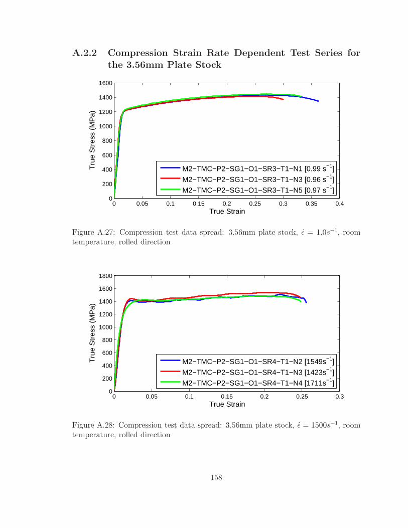
A.2.2 Compression Strain Rate Dependent Test Series for
the 3.56mm Plate Stock
0 0.05 0.1 0.15 0.2 0.25 0.3 0.35 0.40
200
400
600
800
1000
1200
1400
1600
True Strain
Tru
e S
tres
s (M
Pa)
M2−TMC−P2−SG1−O1−SR3−T1−N1 [0.99 s−1]
M2−TMC−P2−SG1−O1−SR3−T1−N3 [0.96 s−1]
M2−TMC−P2−SG1−O1−SR3−T1−N5 [0.97 s−1]
Figure A.27: Compression test data spread: 3.56mm plate stock, ǫ = 1.0s−1, roomtemperature, rolled direction
0 0.05 0.1 0.15 0.2 0.25 0.30
200
400
600
800
1000
1200
1400
1600
1800
True Strain
Tru
e S
tres
s (M
Pa)
M2−TMC−P2−SG1−O1−SR4−T1−N2 [1549s−1]
M2−TMC−P2−SG1−O1−SR4−T1−N3 [1423s−1]
M2−TMC−P2−SG1−O1−SR4−T1−N4 [1711s−1]
Figure A.28: Compression test data spread: 3.56mm plate stock, ǫ = 1500s−1, roomtemperature, rolled direction
158

A.2.3 Compression Temperature Dependent Test Series for
the 6.35mm Plate Stock
0 0.05 0.1 0.15 0.2 0.25 0.3 0.35 0.4 0.45 0.50
200
400
600
800
1000
1200
1400
1600
1800
True Strain
Tru
e S
tres
s (M
Pa)
M2−TMC−P3−SG1−O1−SR3−T5−N1 [−51.0oC]
M2−TMC−P3−SG1−O1−SR3−T5−N2 [−52.4oC]
M2−TMC−P3−SG1−O1−SR3−T5−N3 [−49.9oC]
M2−TMC−P3−SG1−O1−SR3−T5−N4 [−52.3oC]
Figure A.29: Compression test data spread: 6.35mm plate stock, ǫ = 1.0s−1, −50C,rolled direction
A.2.4 Compression Strain Rate Dependent Test Series for
the 12.7mm Plate Stock
0 0.05 0.1 0.15 0.2 0.25 0.30
200
400
600
800
1000
1200
1400
1600
True Strain
Tru
e S
tres
s (M
Pa)
M2−TMC−P4−SG1−O1−SR1−T1−N4
M2−TMC−P4−SG1−O1−SR1−T1−N5M2−TMC−P4−SG1−O1−SR1−T1−N6
Figure A.30: Compression test data spread: 12.7mm plate stock, ǫ = 1.0E − 4s−1,room temperature, rolled direction
159

0 0.05 0.1 0.15 0.2 0.25 0.3 0.350
200
400
600
800
1000
1200
1400
1600
1800
True Strain
Tru
e S
tres
s (M
Pa)
M2−TMC−P4−SG1−O1−SR2−T1−N1
M2−TMC−P4−SG1−O1−SR2−T1−N3M2−TMC−P4−SG1−O1−SR2−T1−N4
Figure A.31: Compression test data spread: 12.7mm plate stock, ǫ = 1.0E − 2s−1,room temperature, rolled direction
0 0.05 0.1 0.15 0.2 0.25 0.3 0.350
200
400
600
800
1000
1200
1400
1600
True Strain
Tru
e S
tres
s (M
Pa)
M2−TMC−P4−SG1−O1−SR3−T1−N2
M2−TMC−P4−SG1−O1−SR3−T1−N4M2−TMC−P4−SG1−O1−SR3−T1−N5
Figure A.32: Compression test data spread: 12.7mm plate stock, ǫ = 1.0s−1, roomtemperature, rolled direction
160

0 0.05 0.1 0.15 0.2 0.250
500
1000
1500
2000
True Strain
Tru
e S
tres
s (M
Pa)
M2−TMC−P4−SG1−O1−SR4−T1−N1 [1474s−1]
M2−TMC−P4−SG1−O1−SR4−T1−N2 [818s−1]
M2−TMC−P4−SG1−O1−SR4−T1−N3 [1473s−1]
Figure A.33: Compression test data spread: 12.7mm plate stock, ǫ = 1500s−1, roomtemperature, rolled direction
0 0.02 0.04 0.06 0.08 0.1 0.12 0.14 0.16 0.18 0.20
500
1000
1500
2000
True Strain
Tru
e S
tres
s (M
Pa)
M2−TMC−P4−SG1−O1−SR5−T1−N2 [4084s−1]
M2−TMC−P4−SG1−O1−SR5−T1−N3 [3879s−1]
M2−TMC−P4−SG1−O1−SR5−T1−N5 [3980s−1]
Figure A.34: Compression test data spread: 12.7mm plate stock, ǫ = 4000s−1, roomtemperature, rolled direction
161

0 0.02 0.04 0.06 0.08 0.1 0.12 0.14 0.16 0.18 0.20
300
600
900
1200
1500
1800
2100
True Strain
Tru
e S
tres
s (M
Pa)
M2−TMC−P4−SG1−O1−SR6−T1−N2 [7616s−1]
M2−TMC−P4−SG1−O1−SR6−T1−N3 [7199s−1]
M2−TMC−P4−SG1−O1−SR6−T1−N4 [7971s−1]
Figure A.35: Compression test data spread: 12.7mm plate stock, ǫ = 7000s−1, roomtemperature, rolled direction
A.2.5 Compression Orientation Dependent Test Series for
the 12.7mm Plate Stock
0 0.05 0.1 0.15 0.2 0.25 0.3 0.35 0.40
200
400
600
800
1000
1200
1400
1600
True Strain
Tru
e S
tres
s (M
Pa)
M2−TMC−P4−SG1−O2−SR3−T1−N1
M2−TMC−P4−SG1−O2−SR3−T1−N2M2−TMC−P4−SG1−O2−SR3−T1−N4
Figure A.36: Compression test data spread: 12.7mm plate stock, ǫ = 1.0s−1, roomtemperature, 45 from rolled
162

0 0.05 0.1 0.15 0.2 0.25 0.3 0.350
200
400
600
800
1000
1200
1400
1600
True Strain
Tru
e S
tres
s (M
Pa)
M2−TMC−P4−SG1−O3−SR3−T1−N3
M2−TMC−P4−SG1−O3−SR3−T1−N4M2−TMC−P4−SG1−O3−SR3−T1−N5
Figure A.37: Compression test data spread: 12.7mm plate stock, ǫ = 1.0s−1, roomtemperature, transverse direction
0 0.05 0.1 0.15 0.2 0.25 0.3 0.35 0.4 0.450
200
400
600
800
1000
1200
1400
1600
True Strain
Tru
e S
tres
s (M
Pa)
M2−TMC−P4−SG1−O4−SR3−T1−N1
M2−TMC−P4−SG1−O4−SR3−T1−N2M2−TMC−P4−SG1−O4−SR3−T1−N3
Figure A.38: Compression test data spread: 12.7mm plate stock, ǫ = 1.0s−1, roomtemperature, −45 from rolled
163

0 0.1 0.2 0.3 0.4 0.5 0.60
200
400
600
800
1000
1200
1400
1600
True Strain
Tru
e S
tres
s (M
Pa)
M2−TMC−P4−SG1−O5−SR3−T1−N1
M2−TMC−P4−SG1−O5−SR3−T1−N2M2−TMC−P4−SG1−O5−SR3−T1−N4
Figure A.39: Compression test data spread: 12.7mm plate stock, ǫ = 1.0s−1, roomtemperature, through direction
A.2.6 Compression Temperature Dependent Test Series for
the 12.7mm Plate Stock
0 0.05 0.1 0.15 0.2 0.25 0.3 0.35 0.40
200
400
600
800
1000
1200
1400
1600
1800
True Strain
Tru
e S
tres
s (M
Pa)
M2−TMC−P4−SG1−O1−SR3−T5−N1 [−52.1oC]
M2−TMC−P4−SG1−O1−SR3−T5−N2 [−49.0oC]
M2−TMC−P4−SG1−O1−SR3−T5−N3 [−51.1oC]
M2−TMC−P4−SG1−O1−SR3−T5−N4 [−49.4oC]
Figure A.40: Compression test data spread: 12.7mm plate stock, ǫ = 1.0s−1, −50C,rolled direction
164
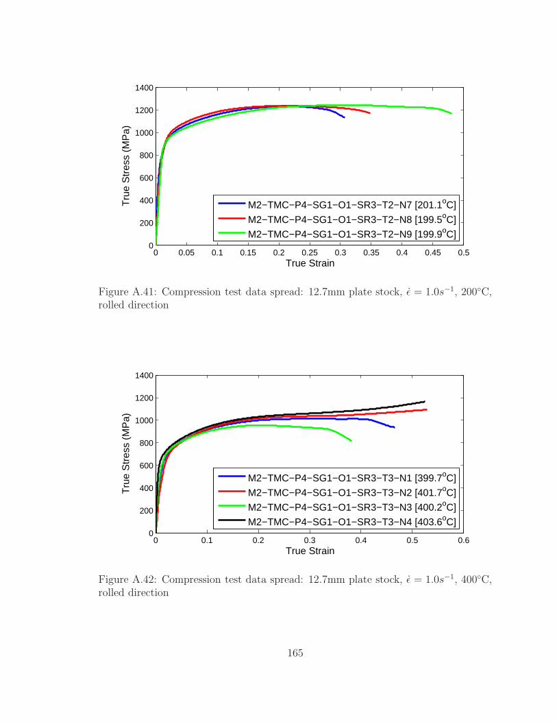
0 0.05 0.1 0.15 0.2 0.25 0.3 0.35 0.4 0.45 0.50
200
400
600
800
1000
1200
1400
True Strain
Tru
e S
tres
s (M
Pa)
M2−TMC−P4−SG1−O1−SR3−T2−N7 [201.1oC]
M2−TMC−P4−SG1−O1−SR3−T2−N8 [199.5oC]
M2−TMC−P4−SG1−O1−SR3−T2−N9 [199.9oC]
Figure A.41: Compression test data spread: 12.7mm plate stock, ǫ = 1.0s−1, 200C,rolled direction
0 0.1 0.2 0.3 0.4 0.5 0.60
200
400
600
800
1000
1200
1400
True Strain
Tru
e S
tres
s (M
Pa)
M2−TMC−P4−SG1−O1−SR3−T3−N1 [399.7oC]
M2−TMC−P4−SG1−O1−SR3−T3−N2 [401.7oC]
M2−TMC−P4−SG1−O1−SR3−T3−N3 [400.2oC]
M2−TMC−P4−SG1−O1−SR3−T3−N4 [403.6oC]
Figure A.42: Compression test data spread: 12.7mm plate stock, ǫ = 1.0s−1, 400C,rolled direction
165

0 0.1 0.2 0.3 0.4 0.5 0.6 0.70
200
400
600
800
1000
True Strain
Tru
e S
tres
s (M
Pa)
M2−TMC−P4−SG1−O1−SR3−T4−N1 [601.6oC]
M2−TMC−P4−SG1−O1−SR3−T4−N2 [599.7oC]
M2−TMC−P4−SG1−O1−SR3−T4−N3 [603.5oC]
Figure A.43: Compression test data spread: 12.7mm plate stock, ǫ = 1.0s−1, 600C,rolled direction
A.2.7 Compression Additional for the 12.7mm Plate Stock
0 0.1 0.2 0.3 0.4 0.5 0.60
200
400
600
800
1000
1200
1400
1600
True Strain
Tru
e S
tres
s (M
Pa)
M2−TMC−P3−SG1−O1−SR1−T1−N1 [Yatnalkar − Machined]
M2−TMC−P3−SG1−O1−SR1−T1−N2 [Yatnalkar − Machined]M2−TMC−P3−SG1−O1−SR1−T1−N4 [Hammer − Machined]M2−TMC−P3−SG1−O1−SR1−T1−N5 [Hammer − Machined]M2−TMC−P3−SG1−O1−SR1−T1−N6 [Hammer − EDM]M2−TMC−P3−SG1−O1−SR1−T1−N7 [Hammer − EDM]M2−TMC−P3−SG1−O1−SR1−T1−N8 [Hammer − EDM]
Figure A.44: Compression test data spread: 6.35mm plate stock, ǫ = 1.0E − 4s−1,room temperature, rolled direction, Researcher Comparison and surface finish Tests
166

0 0.05 0.1 0.15 0.2 0.25 0.30
200
400
600
800
1000
1200
1400
1600
True Strain
Tru
e S
tres
s (M
Pa)
M2−TMC−P4−SG2−O1−SR1−T1−N1 <Plate Loc 1>
M2−TMC−P4−SG2−O1−SR1−T1−N2 <Plate Loc 1>M2−TMC−P4−SG2−O1−SR1−T1−N3 <Plate Loc 1>M2−TMC−P4−SG2−O1−SR1−T1−N4 <Plate Loc 2>M2−TMC−P4−SG2−O1−SR1−T1−N5 <Plate Loc 2>M2−TMC−P4−SG2−O1−SR1−T1−N6 <Plate Loc 2>
Figure A.45: Compression test data spread: 12.7mm plate stock, ǫ = 1.0s−1, roomtemperature, rolled direction, Alternate Geometry
A.3 Shear Test Series
A.3.1 Shear Strain Rate Dependent Test Series for the 12.7mm
Plate Stock
0 0.05 0.1 0.15 0.2 0.250
100
200
300
400
500
600
700
Shear Strain
She
ar S
tres
s (M
Pa)
M2−TMS−P4−SR1−T1−N2
M2−TMS−P4−SR1−T1−N3M2−TMS−P4−SR1−T1−N4M2−TMS−P4−SR1−T1−N5
Figure A.46: Shear test data spread: 12.7mm plate stock, ǫ = 1.0E − 4s−1, roomtemperature, through direction
167

0 0.02 0.04 0.06 0.08 0.1 0.12 0.14 0.16 0.18 0.20
100
200
300
400
500
600
700
Shear Strain
She
ar S
tres
s (M
Pa)
M2−TMS−P4−SR2−T1−N1
M2−TMS−P4−SR2−T1−N2M2−TMS−P4−SR2−T1−N3
Figure A.47: Shear test data spread: 12.7mm plate stock, ǫ = 1.0E − 2s−1, roomtemperature, through direction
0 0.02 0.04 0.06 0.08 0.1 0.12 0.14 0.16 0.18 0.20
100
200
300
400
500
600
700
Shear Strain
She
ar S
tres
s (M
Pa)
M2−TMS−P4−SR3−T1−N1
M2−TMS−P4−SR3−T1−N2M2−TMS−P4−SR3−T1−N3M2−TMS−P4−SR3−T1−N4M2−TMS−P4−SR3−T1−N5
Figure A.48: Shear test data spread: 12.7mm plate stock, ǫ = 1.0s−1, room temper-ature, through direction
168

0 0.02 0.04 0.06 0.08 0.1 0.120
100
200
300
400
500
600
700
Shear Strain
She
ar S
tres
s (M
Pa)
M2−TMS−P4−SR4−T1−N5 [309s−1]
M2−TMS−P4−SR4−T1−N6 [310s−1]
M2−TMS−P4−SR4−T1−N7 [437s−1]
M2−TMS−P4−SR4−T1−N8 [442s−1]
Figure A.49: Shear test data spread: 12.7mm plate stock, ǫ = 500s−1, room temper-ature, through direction
0 0.02 0.04 0.06 0.08 0.1 0.120
100
200
300
400
500
600
700
Shear Strain
She
ar S
tres
s (M
Pa)
M2−TMS−P4−SR5−T1−N6 [1080s−1]
M2−TMS−P4−SR5−T1−N7 [907s−1]
M2−TMS−P4−SR5−T1−N8 [1094s−1]
M2−TMS−P4−SR5−T1−N9 [1140s−1]
M2−TMS−P4−SR4−T1−N10 [884s−1]
Figure A.50: Shear test data spread: 12.7mm plate stock, ǫ = 1500s−1, room tem-perature, through direction
169

A.3.2 Shear Temperature Dependent Test Series for the 12.7mm
Plate Stock
0 0.05 0.1 0.150
100
200
300
400
500
600
700
Shear Strain
She
ar S
tres
s (M
Pa)
M2−TMS−P4−SR3−T5−N1 [−50.1oC]
M2−TMS−P4−SR3−T5−N2 [−51.9oC]
M2−TMS−P4−SR3−T5−N3 [−50.8oC]
M2−TMS−P4−SR3−T5−N4 [−50.7oC]
Figure A.51: Shear test data spread: 12.7mm plate stock, ǫ = 1.0s−1, −50C, throughdirection
0 0.05 0.1 0.15 0.2 0.25 0.3 0.350
100
200
300
400
500
Shear Strain
She
ar S
tres
s (M
Pa)
M2−TMS−P4−SR3−T2−N2 [200.9oC]
M2−TMS−P4−SR3−T2−N3 [199.9oC]
M2−TMS−P4−SR3−T2−N4 [199.9oC]
M2−TMS−P4−SR3−T2−N5 [200.9oC]
Figure A.52: Shear test data spread: 12.7mm plate stock, ǫ = 1.0s−1, 200C, throughdirection
170
0 0.1 0.2 0.3 0.4 0.5 0.60
50
100
150
200
250
300
350
400
Shear Strain
She
ar S
tres
s (M
Pa)
M2−TMS−P4−SR3−T3−N1 [400.0oC]
M2−TMS−P4−SR3−T3−N2 [401.7oC]
M2−TMS−P4−SR3−T3−N3 [401.7oC]
Figure A.53: Shear test data spread: 12.7mm plate stock, ǫ = 1.0s−1, 400C, throughdirection
0 0.1 0.2 0.3 0.4 0.5 0.60
50
100
150
200
250
300
Shear Strain
She
ar S
tres
s (M
Pa)
M2−TMS−P4−SR3−T4−N1 [604.5oC]
M2−TMS−P4−SR3−T4−N2 [612.3oC]
M2−TMS−P4−SR3−T4−N4 [601.6oC]
Figure A.54: Shear test data spread: 12.7mm plate stock, ǫ = 1.0s−1, 600C, throughdirection
171

Appendix B: Experimental Results from the Ti-6Al-4V
Ductile Fracture Test Series
The spread in measured data from the fracture test series are presented here.
All data for the plane stress, plane strain, and axisymmetric tests is presented in a
engineering stress versus engineering strain to normalize the data for slight deviations
in specimen size. Combined loading tests data spread is presented showing 4 different
data sets: (a) are the axial force displacement curves, (b) are the torque angle curves,
(c) are the stress triaxiality versus time, and (d) are the Lode Parameter versus
time. Data spread for the punch tests are presented with force displacement curves.
Discussion of this data was presented in Chapter 4.
172

B.1 Plane Stress Test Series
0 0.05 0.1 0.15 0.20
200
400
600
800
1000
1200
Engineering Strain
Eng
inee
ring
Str
ess
(MP
a)
M2−TMT−P4−SG2−O1−SR2−T1−N2
M2−TMT−P4−SG2−O1−SR2−T1−N3M2−TMT−P4−SG2−O1−SR2−T1−N4
Figure B.1: Fracture test data spread: plane stress notched, notch=14.29mm, 12.7mmplate stock, SR=1.0−2s−1, room temperature, rolled direction
0 0.05 0.1 0.150
200
400
600
800
1000
1200
Engineering Strain
Eng
inee
ring
Str
ess
(MP
a)
M2−TMT−P4−SG3−O1−SR2−T1−N1
M2−TMT−P4−SG3−O1−SR2−T1−N2M2−TMT−P4−SG3−O1−SR2−T1−N3
Figure B.2: Fracture test data spread: plane stress notched, notch=4.76mm, 12.7mmplate stock, SR=1.0−2s−1, room temperature, rolled direction
173

0 0.01 0.02 0.03 0.04 0.05 0.06 0.070
500
1000
1500
Engineering Strain
Eng
inee
ring
Str
ess
(MP
a)
M2−TMT−P4−SG4−O1−SR2−T1−N1
M2−TMT−P4−SG4−O1−SR2−T1−N2M2−TMT−P4−SG4−O1−SR2−T1−N3
Figure B.3: Fracture test data spread: plane ptress notched, notch=0.40mm, 12.7mmplate stock, SR=1.0−2s−1, room temperature, rolled direction
B.2 Axisymmetric Test Series
0 0.05 0.1 0.15 0.2 0.25 0.3 0.350
200
400
600
800
1000
1200
Engineering Strain
Eng
inee
ring
Str
ess
(MP
a)
M2−TMT−P4−SG5−O1−SR2−T1−N1
M2−TMT−P4−SG5−O1−SR2−T1−N2M2−TMT−P4−SG5−O1−SR2−T1−N3M2−TMT−P4−SG5−O1−SR2−T1−N4
Figure B.4: Fracture test data spread: axisymmetric smooth, 12.7mm plate stock,SR=1.0−2s−1, room temperature, rolled direction
174

0 0.05 0.1 0.15 0.2 0.250
200
400
600
800
1000
1200
Engineering Strain
Eng
inee
ring
Str
ess
(MP
a)
M2−TMT−P4−SG6−O1−SR2−T1−N1
M2−TMT−P4−SG6−O1−SR2−T1−N2M2−TMT−P4−SG6−O1−SR2−T1−N3
Figure B.5: Fracture test data spread: axisymmetric notched, notch=34.93mm,12.7mm plate stock, SR=1.0−2s−1, room temperature, rolled direction
0 0.02 0.04 0.06 0.08 0.1 0.12 0.14 0.16 0.18 0.20
200
400
600
800
1000
1200
1400
Engineering Strain
Eng
inee
ring
Str
ess
(MP
a)
M2−TMT−P4−SG7−O1−SR2−T1−N2
M2−TMT−P4−SG7−O1−SR2−T1−N3M2−TMT−P4−SG7−O1−SR2−T1−N4M2−TMT−P4−SG7−O1−SR2−T1−N5
Figure B.6: Fracture test data spread: axisymmetric notched, notch=17.46mm,12.7mm plate stock, SR=1.0−2s−1, room temperature, rolled direction
175

0 0.02 0.04 0.06 0.08 0.1 0.12 0.14 0.16 0.18 0.20
200
400
600
800
1000
1200
1400
Engineering Strain
Eng
inee
ring
Str
ess
(MP
a)
M2−TMT−P4−SG8−O1−SR2−T1−N2
M2−TMT−P4−SG8−O1−SR2−T1−N3M2−TMT−P4−SG8−O1−SR2−T1−N4
Figure B.7: Fracture test data spread: axisymmetric notched, notch=11.9mm,12.7mm plate stock, SR=1.0−2s−1, room temperature, rolled direction
0 0.02 0.04 0.06 0.08 0.1 0.12 0.14 0.16 0.18 0.20
500
1000
1500
Engineering Strain
Eng
inee
ring
Str
ess
(MP
a)
M2−TMT−P4−SG9−O1−SR2−T1−N1
M2−TMT−P4−SG9−O1−SR2−T1−N2M2−TMT−P4−SG9−O1−SR2−T1−N3
Figure B.8: Fracture test data spread: axisymmetric notched, notch=6.75mm,12.7mm plate stock, SR=1.0−2s−1, room temperature, rolled direction
176

0 0.02 0.04 0.06 0.08 0.1 0.12 0.14 0.16 0.18 0.20
500
1000
1500
Engineering Strain
Eng
inee
ring
Str
ess
(MP
a)
M2−TMT−P4−SG10−O1−SR2−T1−N1
M2−TMT−P4−SG10−O1−SR2−T1−N2M2−TMT−P4−SG10−O1−SR2−T1−N3M2−TMT−P4−SG10−O1−SR2−T1−N4
Figure B.9: Fracture test data spread: axisymmetric notched, notch=3.18mm,12.7mm plate stock, SR=1.0−2s−1, room temperature, rolled direction
B.3 Plane Strain Test Series
0 0.02 0.04 0.06 0.08 0.1 0.12 0.14 0.16 0.18 0.20
200
400
600
800
1000
1200
1400
Engineering Strain
Eng
inee
ring
Str
ess
(MP
a)
M2−TMT−P4−SG11−O1−SR2−T1−N1
M2−TMT−P4−SG11−O1−SR2−T1−N2M2−TMT−P4−SG11−O1−SR2−T1−N3
Figure B.10: Fracture test data spread: plane strain smooth, 12.7mm plate stock,SR=1.0−2s−1, room temperature, rolled direction
177

0 0.05 0.1 0.150
200
400
600
800
1000
1200
1400
Engineering Strain
Eng
inee
ring
Str
ess
(MP
a)
M2−TMT−P4−SG12−O1−SR2−T1−N1
M2−TMT−P4−SG12−O1−SR2−T1−N2M2−TMT−P4−SG12−O1−SR2−T1−N3M2−TMT−P4−SG12−O1−SR2−T1−N4
Figure B.11: Fracture test data spread: plane strain notched, notch=12.7mm,12.7mm plate stock, SR=1.0−2s−1, room temperature, rolled direction
0 0.01 0.02 0.03 0.04 0.05 0.06 0.07 0.08 0.09 0.10
200
400
600
800
1000
1200
1400
Engineering Strain
Eng
inee
ring
Str
ess
(MP
a)
M2−TMT−P4−SG13−O1−SR2−T1−N1
M2−TMT−P4−SG13−O1−SR2−T1−N2M2−TMT−P4−SG13−O1−SR2−T1−N3
Figure B.12: Fracture test data spread: plane strain notched, notch=4.76mm,12.7mm plate stock, SR=1.0−2s−1, room temperature, rolled direction
178

B.4 Combined Loading Test Series
0 0.1 0.2 0.3 0.4 0.50
4
8
12
16(a)
Displacement (mm)
Axi
al L
oad
(kN
)
0 2 4 6 80
5
10
15
20
25
30
35(b)
Angle (deg)
Tor
que
(Nm
)
0 20 40 60 800
0.07
0.14
0.21
0.28
0.35
Time (s)
Str
ess
Tria
xial
ity [σ
*]
(c)
0 20 40 60 800
0.3
0.6
0.9
1.2
Time (s)
Lode
Par
amet
er [µ
]
(d)
M2−TMCL−P4−LR1−SR3−T1−N1
M2−TMCL−P4−LR1−SR3−T1−N2M2−TMCL−P4−LR1−SR3−T1−N3
Figure B.13: Combined loading force displacement data spread:, 12.7mm plate stock,σ/τ=1.971, room temperature, rolled direction
179

0 0.1 0.2 0.3 0.4 0.50
2
4
6
8
10
Displacement (mm)
Axi
al L
oad
(kN
)
(a)
0 5 10 15 200
10
20
30
40
50
Angle (deg)T
orqu
e (N
m)
(b)
0 10 20 30 40 500
0.07
0.14
0.21
0.28
0.35
Time (s)
Str
ess
Tria
xial
ity [σ
*]
(c)
0 10 20 30 40 500
0.2
0.4
0.6
0.8
1
1.2
Time (s)
Lode
Par
amet
er [µ
]
(d)
M2−TMCL−P4−LR2−SR3−T1−N1
M2−TMCL−P4−LR2−SR3−T1−N3M2−TMCL−P4−LR2−SR3−T1−N6
Figure B.14: Combined loading stress state parameter data spread:, 12.7mm platestock, σ/τ=0.847, room temperature, rolled direction
180

0 0.1 0.2 0.3 0.4 0.5 0.60
2
4
6
8
10
Displacement (mm)
Axi
al L
oad
(kN
)
(a)
0 5 10 15 20 250
10
20
30
40
50
Angle (deg)T
orqu
e (N
m)
(b)
0 10 20 30 40 50 60−0.1
−0.05
0
0.05
0.1
(c)
Time (s)
Str
ess
Tria
xial
ity [σ
*]
0 10 20 30 40 50 60−0.1
−0.05
0
0.05
0.1
Time (s)
Lode
Par
amet
er [µ
]
(d)
M2−TMCL−P4−LR3−SR3−T1−N2
M2−TMCL−P4−LR3−SR3−T1−N3M2−TMCL−P4−LR3−SR3−T1−N4
Figure B.15: Combined loading stress state parameter data spread:, 12.7mm platestock, σ/τ=0.0, room temperature, rolled direction
181

0 0.05 0.1 0.15 0.2 0.25 0.30
5
10
15
20
25
Displacement (mm)
Axi
al L
oad
(kN
) (a)
0 5 10 15 200
20
40
60
80
100
Angle (deg)T
orqu
e (N
m)
(b)
0 10 20 30 40 50−0.35
−0.28
−0.21
−0.14
−0.07
0
Time (s)
Str
ess
Tria
xial
ity [σ
*]
(c)
0 10 20 30 40 50−1.2
−1
−0.8
−0.6
−0.4
−0.2
0
Time (s)
Lode
Par
amet
er [µ
]
(d)
M2−TMCL−P4−LR4−SR3−T1−N3
M2−TMCL−P4−LR4−SR3−T1−N4M2−TMCL−P4−LR4−SR3−T1−N5
Figure B.16: Combined loading stress state parameter data spread:, 12.7mm platestock, σ/τ=-0.847, room temperature, rolled direction
182

Appendix C: Finite Element Meshes used in the Tension
Specimen Design for the Fracture Characterization Test
Series
The mesh sizes for the simulated fracture experiments are presented here. These
meshes were used in LS-DYNA simulations results of which are presented in Appendix
D. Results from these simulations are used in development of the fracture locus
and presented in Chapter 4. For each of the specimens a constant mesh density of
approximately 65.6 elements/cm is used. The Axisymmetric specimens are shown in
a section view to show the center elements.
183
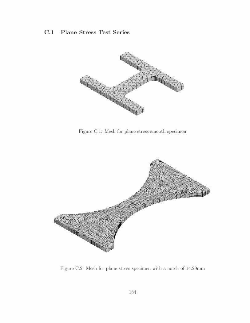
C.1 Plane Stress Test Series
Figure C.1: Mesh for plane stress smooth specimen
Figure C.2: Mesh for plane stress specimen with a notch of 14.29mm
184

Figure C.3: Mesh for plane stress specimen with a notch of 4.76mm
Figure C.4: Mesh for plane stress specimen with a notch of 0.40mm
185

C.2 Axisymmetric Test Series
Figure C.5: Mesh for axisymmetric smooth Specimen (section view)
Figure C.6: Mesh for axisymmetric specimen with a notch of 34.93mm (section view)
186

Figure C.7: Mesh for axisymmetric specimen with a notch of 17.46mm (section view)
Figure C.8: Mesh for axisymmetric specimen with a notch of 11.91mm (section view)
187

Figure C.9: Mesh for axisymmetric specimen with a notch of 6.75mm (section view)
Figure C.10: Mesh for axisymmetric specimen with a notch of 3.18mm (section view)
188

C.3 Plane Strain Test Series
Figure C.11: Mesh for plane strain smooth specimen
Figure C.12: Mesh for plane strain specimen with a notch of 4.76mm
189

Figure C.13: Mesh for plane strain specimen with a notch of 12.70mm
190

Appendix D: Comparison of Experimental Data and
Simulations of Fracture Test Series
The fracture points found from comparing simulations to physical results. The
comparisons of the plane stress, axisymmetric, and plane strain tests are presented
here. The first and second principle strain comparison of the DIC surface strains to
the simulation surface strains. Levels of the respective strains are identical between
the DIC and simulated specimens. The included plots provide a comparison of stress
levels and surface strains. The strains from the center of the simulated values are
also shown, which is where the failure points are taken. The stress triaxialities and
Lode Parameter are displayed as taken from the center element.
Combined loading DIC data and time history is also presented. Strain data is
taken from a DIC point strain on the surface of the specimen near the fracture point.
Simulations are not performed on these specimens because their stress states are only
dependent on axial-torsional loading ratio.
191

D.1 Plane Stress Test Series
Figure D.1: History comparison of simulated and experimental fracture data for theplane stress smooth specimen
192

Figure D.2: History comparison of simulated and experimental fracture data for theplane stress large notch specimen R=14.29mm
193

Figure D.3: History comparison of simulated and experimental fracture data for theplane stress medium notch specimen R=4.76mm
194

Figure D.4: History comparison of simulated and experimental fracture data for theplane stress small notch specimen R=0.40mm
195

D.2 Axisymmetric Test Series
Figure D.5: History comparison of simulated and experimental fracture data for theaxisymmetric smooth specimen
196

Figure D.6: History comparison of simulated and experimental fracture data for theaxisymmetric notched specimen R=34.93mm
197

Figure D.7: History comparison of simulated and experimental fracture data for theaxisymmetric notched specimen R=17.46mm
198

Figure D.8: History comparison of simulated and experimental fracture data for theaxisymmetric notched specimen R=11.91mm
199

Figure D.9: History comparison of simulated and experimental fracture data for theaxisymmetric notched specimen R=6.75mm
200
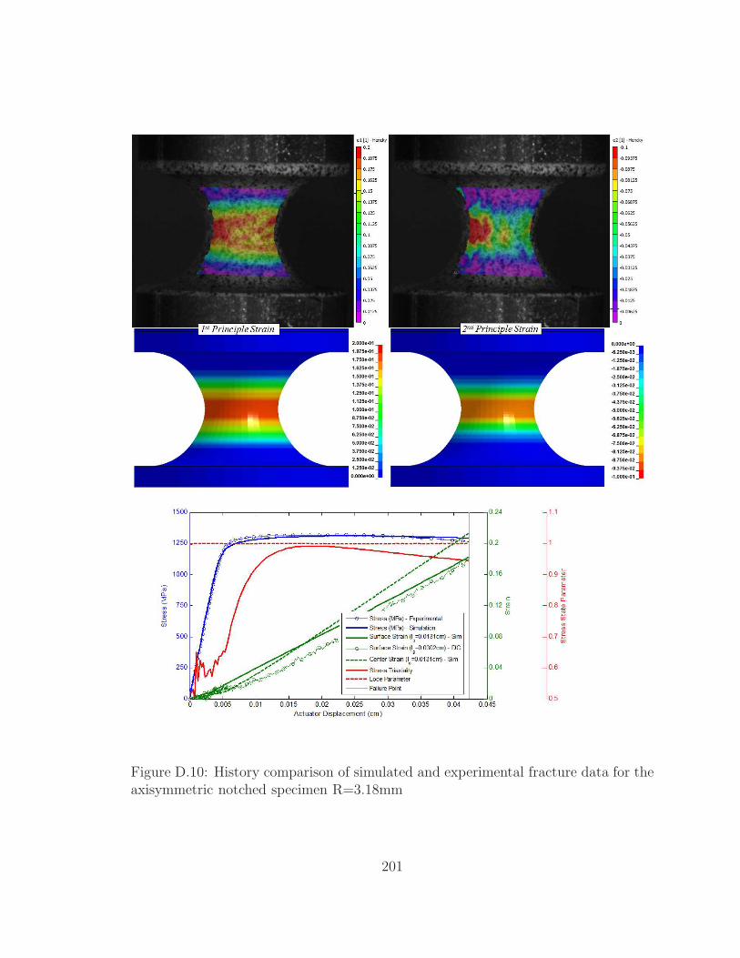
Figure D.10: History comparison of simulated and experimental fracture data for theaxisymmetric notched specimen R=3.18mm
201

D.3 Plane Strain Test Series
Figure D.11: History comparison of simulated and experimental fracture data for theplane strain smooth
202

Figure D.12: History comparison of simulated and experimental fracture data for theplane strain large notch R=12.7mm
203

Figure D.13: History comparison of simulated and experimental fracture data for theplane strain small notch R=4.76mm
204

D.4 Combined Loading Test Series
Figure D.14: history of experimental fracture data for the combined loading σ/τ =1.971
205
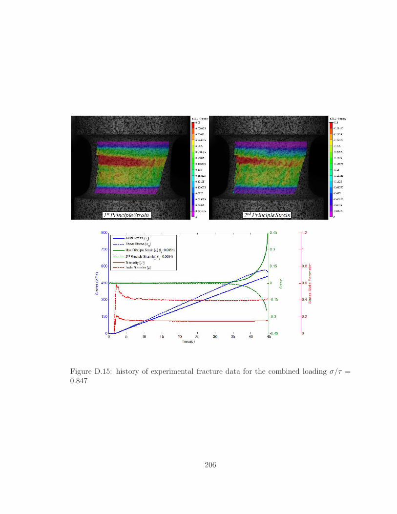
Figure D.15: history of experimental fracture data for the combined loading σ/τ =0.847
206

Figure D.16: history of experimental fracture data for the combined loading σ/τ =0.00
207

Figure D.17: history of experimental fracture data for the combined loading σ/τ =−0.847
208

Appendix E: Additional Views of the Fracture Locus for
Ti-6Al-4V
Additional view of the fracture locus for Ti64 will be presented here. This locus has
been developed with the methods presented in Chapter 2. Detailed results from each
of the tests are presented in Chapter 4. Plane stress, axisymmetric, plane strain, and
combined loading results are displayed with a circle, square, triangle, and diamond
respectively. The x, y, and z axes represent the stress triaxiality, Lode parameter,
and plastic fracture strains respecitvely.
209

Figure E.1: Fracture locus for Ti-6Al-4V in the stress triaxiality - Lode parameterplane
Figure E.2: Fracture locus for Ti-6Al-4V in the stress triaxiality - failure strain plane
210

Figure E.3: Fracture locus for Ti-6Al-4V in the Lode parameter - failure strain plane
Figure E.4: Three dimensional view of the Ti-6Al-4V fracture locus
211

Bibliography
[1] R. Hill. The Mathematical Theory of Plasticity. Oxford University Press, London,1964.
[2] LSTC. LS-DYNA Keyword User’s Manual, Volumes I and II, Version 971.
Livermore, CA, 2007.
[3] ABAQUS. Abaqus Features, 2012.
[4] G.R. Johnson and W.H. Cook. A constitutive model and data for metals sub-jected to large strains, high strain rates, and high temperatures. Proceedings of
the 7th International Symposium on Ballistics, April 1983.
[5] G.R. Johnson and W.H. Cook. Fracture characteristics of three metals sub-jected to various strains, strain rates, temperatures, and pressures. Engineering
Fracture Mechanics, 21(1):31–48, 1985.
[6] NTSB. Uncontained engine failure, delta air line flight 1288, mcdonnell-douglassmd-88 n927da pensacola, fla., july 6, 1996. Aircraft Accident Report AAR-98-01,
July 1996.
[7] NTSB. United airlines flight 232 mcdonnell douglass dc-10-10 sioux gatewayairport sioux city, iowa july 1989. Aircraft Accident Report AAR-90-06, July
1989.
[8] NTSB. Fail safe design requirements and fatures, regulatory requrements. AIAAConference, July 2004.
[9] Kivanc Sengoz, Steve Kan, and Chip Queitzsch. Fan rig model status update.
FAA Meeting Update, January 2012.
[10] C.E. Frankenberger. Large engine uncontained debris analysis. Final Report to
the U.S. Department of Transportation, Federial Aviation Administration, Report
No. DOT/FAA/AR-99/11, May 1999.
[11] Rodney Boyer and Gerhard Welsch. Material Properties Handbook - Titanium
Alloys. ASM International, 1994.
212

[12] Ravi Yatnalkar. Experimental investigation of plastic deformation of ti-6al-4vunder various loading conditions. Master’s thesis, The Ohio State University,
2010.
[13] G.L. Wulf. High strain rate compression of titanium and some titanium alloys.
International Journal of Mechanical Sciences, 21:713–718, July 1976.
[14] P.S. Follansbee and G.T. Gray III. An analysis of the low temperature, low and
high strain-rate deformation of ti-6al-4v. Metallurgical Transactions A, 20A:863–874, 1989.
[15] Woei-Shyan Lee and Ming-Tong Lin. The effects of strain rate and temperatureon the compressive deformation behaviour of ti-6al-4v alloy. Journal of Materials
Processing Technology, 71:235–246, 1995.
[16] Woei-Shyan Lee and Chi-Feng Lin. Plastic deformation and fracture behaviour ofti-6al-4v alloy loaded with high strain rate under various temperatures. Materials
Science and Engineering, pages 48–59, 1998.
[17] W.S. Lee, C.F. Lin, and S.Z. Huang. Effect of temperature and strain rate on the
shear properties fo ti-6al-4v alloy. Journal of Mechanical Engineering Science,220:127–136, 2005.
[18] J.R. Rice and D.M. Tracey. On the ductile enlargement of voids in triaxial stressfields. Journal of the Mechanics and Physics of Solids, 17:201–217, 1969.
[19] Y. Bau and T. Wierzbicki. On fracture locus in the equivalent strain and stresstriaxiality space. International Journal of Mechanical Sciences, 46:81–98, 2004.
[20] L. Xue. Damage accumulation and fracture initiation in uncracked ductile solids
subjected to triaxial loading. International Journal of Solids and Structures,44:5163–5181, 2007.
[21] Jeremy Seidt. Plastic Deformation and Ductile Fracture of 2024-T351 Aluminumunder Various Loading Conditions. PhD thesis, The Ohio State University, 2010.
[22] D. Lesuer. Experimental investigations of material models for ti-6al-4v titaniumand 2024-t3 aluminum. FAA Technical Report, 2000.
[23] A.S. Milani, W. Dabboussi, J.A. Nemes, and R.C. Abeyarate. An improvedmulti-objective identification of johnsoncook material parameters. International
Journal of Impact Engineering, 36, 2009.
[24] I. Barsoum and J. Faleskog. Rupture mechanics in combined tension and shear -
experiments. International Journal of Solids and Structures, 44:1768–1786, 2007.
213

[25] M. Sutton, J.J. Orteu, and H.W. Schreier. Image Correlation for Shape, Motionand Deformation Measurements. Springer, New York, NY, 2009.
[26] P.W. Bridgman. Studies in large plastic flow and fracture, with special emphasison the effect of hydrostatic pressure. Harvard University Press, 1964.
[27] M. Buyuk, P. DuBois, J. He, and S. Kan. Procedure for the determiniation ofthe specimen geometries. Presentation Slides May 7th, 2010.
[28] B. Dodd and Y. Bai. Ductile Fracture and Ductility with Applications to Metal-working. Harcourt Brace Jovanovich Publishers, London, 1987.
[29] H. Kolsky. Stress waves in solids. Journal of Sound and Vibration, 1:88–110,
1963.
[30] G. T. Gray III. Classic split-hopkinson pressure bar testing. ASM Handbook,
8:462–476, 2000.
[31] G.H. Staab and A. Gilat. A direct-tension split hopkinson bar for high strain-rate
testing. Experimental Mechanics, 31:232–235, 1991.
[32] A. Gilat. Torsional kolsky bar testing. ASM Handbook, 8, 2000.
[33] Inc. Correlated Solutions. Correlated solutions: Non-contacting measurementsolutions. < http : //www.correlatedsolutions.com >, Nov 2012.
[34] D. Sandwell. Biharmonic spline interpolation of geos-3 and seasat altimeter data.Geophysical Research Letters, 14:139–142, 1987.
[35] J.S. Lyons, J. Liu, and M.A. Sutton. High-temperature deformation measure-
ments using digital-image correlation. Society for Experimental Mechanics, 1995.
[36] B.M.B. Grant, H.J. Stone, P.J. Withers, and M Preuss. High-temperature strain
field measurement using digital image correlation. Journal of Strain Analysis,44:263–271, 2008.
[37] Bing Pan, Dafang Wu, Zhaoyang Wang, and Yong Xia. High-temperature digi-tal image correlation method for full-field deformation meaurements at 1200c.
Measurment Science and Technology, 22, 2011.
[38] Tiffen. Tiffen announces the solution to ir pollution. http: // www. tiffen.
com/ press\ _release\ _Hot\ _Mirror\ _IRND. htm , April 2008.
[39] E.W. Collings. Material Properties Handbook: Titanium Alloys. ASM Interna-
tional, Materials Park, OH, 1994.
214
Top Related