


Languages
Pages
Legal


Phase Behavior of the Restricted Primitive Model and Square-Well Fluids from
Monte Carlo Simulations in the Grand Canonical Ensemble
Gerassimos Orkoulas and Athanassios Z. Panagiotopoulos*
School of Chemical Engineering, Cornell University, Ithaca, NY 14853-5201
and
Institute for Physical Science and Technology and Department of Chemical Engineering,
University of Maryland, College Park, MD 20742-2431
ABSTRACT
Coexistence curves of square-well fluids with variable interaction width and of the restricted
primitive model for ionic solutions have been investigated by means of grand canonical Monte
Carlo simulations aided by histogram reweighting and multicanonical sampling techniques. It is
demonstrated that this approach results in efficient data collection. The shape of the coexistence
curve of the square-well fluid with short potential range is nearly cubic. In contrast, for a system
with a longer potential range, the coexistence curve closely resembles a parabola, except near the
critical point. The critical compressibility factor for the square-well fluids increases with
increasing range. The critical behavior of the restricted primitive model was found to be
consistent with the Ising universality class. The critical temperature was obtained as
Tc=0.0490±0.0003 and the critical density ρc=0.070±0.005, both in reduced units. The critical
temperature estimate is consistent with the recent calculation of Caillol et al. [J. Chem. Phys.,
107, 1565, 1997] on a hypersphere, while the critical density is slightly lower. Other previous
simulations have overestimated the critical temperature of this ionic fluid due to their failure to
account for finite-size effects in the critical region. The critical compressibility factor (Zc=Pc /
ρcTc) for the ionic fluid was obtained as Zc=0.024±0.004, an order of magnitude lower than for
non-ionic fluids.
Revised version submitted to J. Chem. Phys., Oct. 7, 1998; 21 pages +10 figures
*Author to whom correspondence should be addressed at the University of Maryland.E-mail: [email protected]

2
I. INTRODUCTION
Significant methodological progress has been made over the years in the development of
Monte Carlo algorithms capable of predicting phase equilibrium properties for model
systems1,2,3,4. A commonly used simulation method is the Gibbs Ensemble Monte Carlo method
of Panagiotopoulos1. This method utilizes two physically detached but thermodynamically
connected boxes representative of the coexisting phases. Particle transfers and volume
exchanges between the boxes lead to establishment of phase equilibrium.
The Gibbs ensemble method provides information at a single temperature for which the
simulation was performed. The calculations must be repeated at different temperatures in order
to cover the entire coexistence range, which is, in principle, a tedious and time consuming
process. An alternative technique by Ferrenberg and Swendsen5 has potentially higher efficiency
by increasing the amount of information that can be obtained from a single simulation. This is
achieved by forming histograms of fluctuating observables during the course of the simulation.
These histograms provide the means of calculating thermodynamic properties of the state under
investigation as well as of neighboring states. The latter can be achieved by extrapolating
(reweighting) the histogram of the reference state. This histogram reweighting procedure is
particularly useful in the critical region where, owing to the large fluctuations, a single
simulation covers wide ranges of the associated parameter space.
All molecular simulation techniques encounter difficulties in the critical region since they
utilize finite systems and cannot capture the divergence of the correlation length. Finite-size
scaling techniques, however, afford accurate estimates of infinite-volume critical points from
simulations of systems of finite size. These methodologies have mainly been applied to lattice-
based magnetic systems6,7,8,9 but they have recently been extended to off-lattice fluids by
explicitly accounting for the lack of symmetry between the coexisting phases10. These theories
are based on the observation that, at criticality, the distribution functions of certain fluctuating
observables assume universal and scale invariant forms. These universal (also known as scaling)
functions are the same for every fluid in a given universality class. This fact can be utilized to
obtain accurate estimates of critical points, provided that these functions are independently
known.
In this work, we have carried out grand canonical Monte Carlo simulations aided by
histogram reweighting, multicanonical sampling and finite-size scaling techniques to obtain the

3
coexistence curves and the associated critical points of square-well fluids and of the restricted
primitive model. We begin by defining the model potentials and we also give some necessary
details on the methods used. We then present results for the systems studied and comparisons
with previous data and finally conclude by discussing potential advantages, possible drawbacks
and future applications of the computational methods used in this work.
II. MODELS STUDIED
Systems interacting according to square-well (SW) potentials have been studied
extensively,11,12,13,14,15 since they constitute the simplest off-lattice fluids that exhibit phase
separation. The pair potential between particles i and j, separated by a distance rij, is defined by
σλ>λσ≤<σ
σ≤ε−
∞=
ij
ij
ij
ij
r
r
r
U
0
(1)
where ε and λ are the interaction range and strength respectively. As is common in simulations,
appropriate reduced quantities (temperature T* and density ρ* ) can be defined by scaling with the
energy parameter ε, and the particle diameter σ, e.g. T*=kBT/ε and ρ*=ρσ3 where kB is
Boltzmann’s constant (kB=1.381·10-23J/K). In the remainder of this paper, we omit asterisks
from reduced quantities for the sake of simplicity. Knowledge of the phase behavior is of
considerable theoretical importance since by varying the interaction range, λ, this model can
interpolate between the hard-sphere and the long-range van der Waals fluid.
The restricted primitive model (RPM) consists of a collection of hard spheres of equal
diameter σ, half of them carrying positive charge and the other half negative that interact via a
Coulomb potential. The charged spheres are allowed to move in a structureless background
characterized by dielectric constant D. In accordance with Coulomb’s law the pair potential is
taken to be
U DD
z z e
rr
rij
i j
ijij
ij=
∞
≥<
1
4 0
2
πσσ (2)
where zie and zje are the charges of ions i and j respectively (|zi|=|zj|), e is the charge of the
electron (e=1.602⋅10-19C), D is the dielectric constant of the medium and D0 is the dielectric

4
permeability of the vacuum (D0=8.85⋅10-12C2N-1m-2). Reduced temperature and density are
defined by scaling with the Coulomb energy between two ions at contact, e2/4πDD0σ, and the
size parameter, σ.
There have been numerous theoretical16 and numerical17 attempts aimed on establishing
the RPM coexistence curve and associated critical point. Despite these efforts, there are still
significant disagreements among results of different investigations. One of the reasons for these
differences is the strong Coulomb force that causes the system to associate and renders both
theoretical and numerical investigations of the system significantly harder than corresponding
non-ionic fluids. Recent Monte Carlo simulations18,19,20 as well as theoretical advances21,22 have
resulted in estimates for Tc≈0.055 and ρc≈0.03-0.05, although there is considerable scatter among
results from different investigations. The question of the universality class to which this model
belongs still remains open. For fluids for which ionic species are present, one generally
distinguishes between solvophobic and Coulombic phase separation23. Solvophobic phase
separation is driven primarily by the short-range solvent-salt or vacuum-salt interactions,
whereas Coulombic phase separation is driven be the strong electrostatic forces. Experimental
studies of ionic fluids have found Ising behavior24,25 in some systems, classical mean-field26,27 in
others and crossover behavior in yet other systems28,29. Recent experiments, however, do not
seem to support the classical or even crossover scenario from classical to Ising behavior30,31.
III. SIMULATION METHODOLOGIES
A. Histogram reweighting and multicanonical sampling
The idea of sorting the simulation data in the form of histograms of fluctuating
observables in order to obtain properties of the state under investigation and neighboring states is
quite old32. It had not been used in investigations of subcritical and near-critical coexistence
properties of fluids until the work of Ferrenberg and Swendsen5 for lattice-based magnetic
systems. In a grand canonical Monte Carlo simulation at fixed chemical potential µ0,
temperature T0 (or inverse temperature K0=1/kBT0), and volume V (or linear size L=V1/3), the joint
probability of observing a given number of particles N (or density ρ=N/V) and energy E is
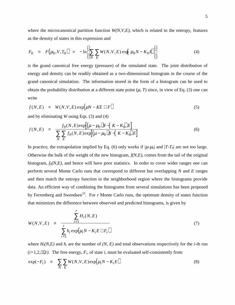
( )f N E W N V E N K E F0 0 0( , ) ( , , )= − +exp µ0 (3)
5
where the microcanonical partition function W(N,V,E), which is related to the entropy, features
as the density of states in this expression and
( ) ( )F F V T W N V E N K EEN
0 0 0 0 0= = − −
∑∑µ µ, , ln ( , , ) exp (4)
is the grand canonical free energy (pressure) of the simulated state. The joint distribution of
energy and density can be readily obtained as a two-dimensional histogram in the course of the
grand canonical simulation. The information stored in the form of a histogram can be used to
obtain the probability distribution at a different state point (µ, T) since, in view of Eq. (3) one can
write
( )f N E W N V E N KE F( , ) ( , , )= − +exp µ (5)
and by eliminating W using Eqs. (3) and (4)
( ) ( )[ ]( ) ( )[ ]f N E
f N E N K K E
f N E N K K EEN
( , )( , )exp
( , )exp=
− − −
− − −∑∑0 0 0
0 0 0
µ µµ µ
(6)
In practice, the extrapolation implied by Eq. (6) only works if |µ-µ0| and |T-T0| are not too large.
Otherwise the bulk of the weight of the new histogram, f(N,E), comes from the tail of the original
histogram, f0(N,E), and hence will have poor statistics. In order to cover wider ranges one can
perform several Monte Carlo runs that correspond to different but overlapping N and E ranges
and then match the entropy function in the neighborhood region where the histograms provide
data. An efficient way of combining the histograms from several simulations has been proposed
by Ferrenberg and Swendsen33. For r Monte Carlo runs, the optimum density of states function
that minimizes the difference between observed and predicted histograms, is given by
( )W N V E
H N E
h N K E F
ii
r
i i i ii
r( , , )
( , )
exp
=− +
=
=
∑
∑1
1
µ(7)
where Hi(N,E) and hi are the number of (N, E) and total observations respectively for the i-th run
(i= 1,2,⋅⋅⋅,r). The free energy, Fi, of state i, must be evaluated self-consistently from
( )exp( ) ( , , )exp− = −∑∑F W N V E N K Ei i iEN
µ (8)

6
In the context of investigating phase transitions through histogram reweighting
Ferrenberg and Swendsen5 recommend performing simulations in the near-critical region. This
is because the histograms obtained are broad due to the large fluctuations that characterize the
neighborhood of the critical point. It is well known34,35 that the grand canonical density
distribution associated with subcritical temperatures and near-coexistence chemical potentials,
attains a characteristic double-peaked structure. The two peaks are associated with stable (or
metastable) phases whereas the minimum between them can be attributed to the formation of
interfaces36.
Far below the critical point, a conventional grand canonical simulation will thus
encounter serious ergodicity problems due to the size of the barrier that separates the two bulk
phases. The multicanonical ensemble approach37, however, overcomes these difficulties by
artificially enhancing the otherwise infrequent transitions between the bulk phases. The
improvement is achieved by sampling not from the physical density distribution, f(ρ)∝exp(µρV),
but from a modified one, π(ρ), that is nearly-flat throughout the entire region. The modified
distribution, π(ρ), is related to the physical one, f(ρ), through a weight function g(ρ)
π ρ ρ ρ( ) ( ) ( )= ⋅g f (9)
It is apparent that the choice g(ρ)=1/f(ρ) will result in uniform sampling throughout the density
range targeted for study. One clearly needs a prior estimate of the density distribution f(ρ) in
order to use it as a preweigthing function. This estimate, however, can be readily obtained from
histogram reweigthing of a near-critical density distribution. The latter can be easily obtained
since the barrier associated to the formation of interfaces is small in the critical region. Once
uniform sampling has been achieved, the improved grand canonical density histogram, f(ρ), can
be obtained from the measured one, π(ρ), by dividing out the preweighting function g(ρ)
f g( )( )
( )ρ π ρρ= (10)
This procedure can then be repeated by extrapolating the improved density distribution at even
lower temperatures and using its inverse as a new weight function. Closely related to the
multicanonical ensemble technique are the methods of entropic sampling38, expanded
ensembles39 and simulated tempering40.

7
B. Finite-Size Scaling
In the critical region, the correlation length ξ grows very large and often exceeds the
linear size L of the finite system. For such a case, the singularities and discontinuities that
characterize critical behavior in the thermodynamic limit are smeared out and shifted. The
infinite-volume critical point of a system can, however, be extracted from finite systems by
examining the size dependence of certain thermodynamic observables. Fisher and coworkers
first developed this methodology which is known as finite-size scaling41.
The finite-size scaling approach that has been used in this work is the one proposed by
Bruce and Wilding10 that accounts for the lack of symmetry between the coexisting phases. Due
to the absence of particle-hole symmetry, the scaling fields comprise linear combinations of the
coupling K=1/kBT and chemical potential differences42
( )( )
τ µ µµ µ
= − + −= − + −
K K s
h r K Kc c
c c(11)
where τ is the thermal scaling field and h is the ordering scaling field. The subscript c signifies
value at criticality. Parameters s and r are system specific quantities that control the degree of
field mixing. r is the limiting critical gradient of the coexistence curve in the µ-K plane42. On
the other hand, s controls the degree at which the chemical potential features in the thermal
scaling field τ.42 This field mixing effect is manifested in the widely observed singularity of the
coexistence curve diameter of fluids.43,44,45
Associated with these scaling fields are the scaling operators M and E that are found10 to
comprise linear combinations of the particle density ρ and the energy density u=E/V,
( )( )
0VU
V X
(VU
X U
=−
−
=−
−
�
�
�
�
ρ
ρ(12)
For systems possessing the symmetry of the Ising model, M is simply the magnetization whereas
E is the energy density. General finite-size scaling arguments10,36,46 predict that at criticality the
probability distributions PL(M) and PL(E) exhibit scaling behavior of the form
( ) ( )( ) ( )
3 0 $ / 3 $ / 0
3 ( % / 3 % / (
/ 0
/ (
=
=− −
βν
βν
αν
αν
δ
δ
� � � �� �
(13)

8
where α, β, and ν are the standard critical point exponents. δM and δE signify deviations from
criticality ie. δM=M-Mc. The functions PM* and PE
* are universal, i.e., the same for every fluid
in a given universality class while A and B are non-universal (system specific) constants.
For the Ising universality class, these scaling functions can be readily obtained as
histograms by Monte Carlo simulation at the known critical point of the Ising model47.
Analytical approximations have also become available recently48. In order to estimate the
critical point of a fluid of the Ising class one can obtain the distribution PL(M) and then (through
histogram reweighting) search for the point for which PL(M) collapses onto PM*.
IV. THE PHASE BEHAVIOR OF SQUARE-WELL FLUIDS
We have studied the coexistence region of the square-well fluids with interaction range, λ,
of 1.5 and 3, by performing grand canonical Monte Carlo simulations aided by histogram
reweighting and finite-size scaling techniques. The simulations were implemented according to
the algorithm of Norman and Filinov49. For each case, six linear sizes were utilized: L=6, 8, 10,
12, 15 and 18σ. In order to facilitate computations, the simulation volume, V=L3, was
partitioned into cubic cells of size λσ. This approach ensures that the interactions of the particles
at a given cell extend at most to the 26 neighboring cells. The observables recorded were the
density, ρ, the energy density, u, and the histogram of the joint distribution f(ρ,u). The length of
the runs was 50-300⋅106 configurations depending of the system size and the density range
covered. Particle transfers were attempted with frequency 90% (45% insertions and 45%
removals respectively) and particle displacements with frequency 10%.
In order to initiate the investigations, we performed a series of very short runs for the
smaller system sizes (L=6 and 8σ). In these runs, the temperature and chemical potential were
tuned until the density distribution f(ρ)=∫f(ρ,u)du exhibited a double peaked structure with a
shallow minimum. A longer run was then performed in order to accumulate better statistics. To
obtain the critical point, we utilized the matching condition of the order parameter probability
distribution PL(M) onto its limiting form PM*. The histogram of PL(M) was obtained from f(ρ,u)
using M=ρ-su and integrating over the energy fluctuations. The process was repeated (by
changing T, µ, and s through histogram reweighting) until satisfactory collapse onto PM* was
obtained. The result of applying this procedure for the square-well fluid with λ=1.5 and L=8σ is

9
shown in Fig. 1. The estimates for the critical temperature and chemical potential for this system
size were Tc(L)=1.220, µc(L)=-2.9518.
Using the small-L critical point estimate we performed additional simulations for larger
system sizes in order to implement finite-size scaling analysis. The critical parameters were
found to be L-dependent because of corrections to scaling. Similar size dependence was also
found by Wilding in the study of the Lennard-Jones fluid50 that showed that it is possible to
obtain an estimate of the infinite-volume critical point by including the leading correction-to-
scaling exponent. The apparent critical temperature Tc(L) deviates from the infinite-volume limit
Tc(∞) as
νθ /)1()()( +−∝∞− LTLT cc (14)
where θ and ν are the correction-to-scaling and correlation length exponents respectively. Their
values have been estimated to be θ≈0.54 and ν≈0.629 for the 3D Ising class51,52. The critical
temperature of the infinite system can be determined from a least-squares fit. The critical density
can also be obtained from scaling considerations. The L-dependent critical density, ρc(L),
obtained as the first moment of the density distribution at µc(L) and Tc(L), is extrapolated to the
thermodynamic limit according to50
να−−∝∞ρ−ρ /)1()()( LL cc (15)
where α(≈0.11)51,52 is the exponent associated with the divergence of the heat capacity. The
dependence of the critical point parameters on the linear system dimension is shown in Fig. 2 for
the square-well fluid with λ=3. The infinite-volume critical point parameters are obtained by a
least-squares fit. Our results for the critical point parameters extrapolated to the limit of infinite
system size are summarized in Table I.
In order to obtain subcritical coexistence information, we utilized the near-critical
coexistence simulations augmented with additional runs for very low and high densities in order
to improve statistics and cover even wider ranges of the associated parameter space (µ and T).
For very low temperatures a few multicanonical simulations were also employed according to
the procedure outlined in the previous section. The weight (or bias) function g(ρ) that was used
in the multicanonical simulations was obtained from the near-critical density distributions by
histogram reweighting.

10
Our results for the coexistence densities of the square-well fluids are given in Figs. 3 and
4. The equal weight construction53 was used to obtain the coexistence chemical potential for a
given temperature. Saturated vapor and liquid densities were determined from the first moment
under each peak of the density distribution that corresponds to coexistence. The large number of
points obtained is a consequence of the histogram reweighting. The combination of data in one
histogram, the subsequent reweighting, and the coexistence point location constitute a minute
faction of the total computational effort. One can then obtain information for a large number of
thermodynamic states, as is apparent in Figs. 3 and 4, at little extra cost. In the framework of the
histogram reweighting scheme, it is also more convenient to utilize small system sizes in order to
extrapolate over wide regions of the associated parameter space. As Figs. 3 and 4 indicate, for T
not to close to Tc, the coexisting densities are practically independent on the system size L.
In Fig. 3, our grand canonical data for λ=1.5 are compared with the results of Vega et
al.12 which were obtained by Gibbs ensemble Monte Carlo simulations. While the agreement is
rather satisfactory, the grand canonical Monte Carlo results for the coexistence densities, appear
to be more consistent than the scattered Gibbs ensemble data. The likely explanation is the
quality of Monte Carlo sampling. A grand canonical simulation in the two-phase region samples
the entire density domain with an average acceptance rate of 20-25% for the particle transfers.
In contrast, the Gibbs ensemble random walk, which concentrates on sampling the region around
the peaks of the density distribution, yields low acceptance rates (<5%)1 for particle transfers
between the coexisting phases. Due to the coupling of the two simulation boxes in the Gibbs
methodology, trial moves that modify the number of particles or the volume must produce a
favorable change in both boxes in order for the overall step to be accepted. The previous
reasoning indicates that Monte Carlo sampling in the grand canonical ensemble is more efficient
than in the Gibbs ensemble.
Recently, Brilliantov and Valleau54 have performed a numerical study of the coexistence
region of the short-ranged (λ=1.5) square-well fluid. They have used a computational technique
known as density (or thermodynamic) scaling Monte Carlo2. Their estimate of the infinite-
system size critical point, Tc≈1.22±0.01, is in agreement within simulation uncertainty with our
estimate (Tc=1.2180±0.0003). The grand canonical Monte Carlo approach used in the present
study allows for calculations involving larger system sizes and results in smaller statistical
uncertainties for the infinite-system critical point parameters. In addition, the grand canonical

11
approach allows studies at highly subcritical temperatures, at which the difference in density
between the coexisting phases hampers efficient sampling in density scaling Monte Carlo.
Otherwise, equivalent thermodynamic property information is obtained from the two approaches.
To investigate the phase behavior of the square-well fluid with interaction range of λ=3,
Benavides et al.15 performed interfacial molecular dynamics simulations of a fluid confined
between two parallel hard walls. While these interfacial simulations can provide valuable
information about the vapor-liquid interface, they require a large number of particles in order to
yield a stable interface and minimize the effect of confinement. The grand canonical simulations
appear to provide more accurate results with much smaller system sizes, as is apparent in Fig. 4.
A point that merits special attention is the shape of the coexistence curves of the square-
well fluids. The coexistence envelope of the square-well fluid with short-ranged intermolecular
interaction is nearly cubic in shape, a point also emphasized by Vega et al.14. In contrast, the
phase boundary of the square-well fluid with somewhat longer interaction width, appears to be
parabolic in shape away from Tc. Its critical point, however, is expected to be of the Ising type,
as for all systems with interactions of finite range and a scalar order parameter. This behavior
implies a crossover from asymptotic Ising behavior to classical mean-field behavior away from
the critical point. The primary factor for these crossover phenomena is the long range of the
interactions which can suppress the long-range critical fluctuations. Similar crossover
phenomena have also been seen in in simulation studies of two-dimensional spin systems with
extended interaction ranges55. Theoretical attempts to investigate the nature of these phenomena
in fluids and fluid mixtures have appeared recently56,57.
The temperature dependence of the vapor pressure curve for these two fluids is given in
Figs. 5 and 6. Simulation uncertainties are smaller than the symbol size. For a given
temperature, the area under each peak of the coexistence density distribution was calculated and
a quantity proportional to the partition function was thus obtained. The pressure, within an
additive constant, was subsequently obtained from the partition function. The additive constant
was estimated by considering a reference state of known pressure, the gas at very low density,
which obeys the ideal gas law. Our results for the pressure of the of λ=1.5 system are consistent
with those of Brilliantov and Valleau.54 Results of Brilliantov and Valleau for N=256 shown in
Fig. 5 were terminated at the infinite-system estimated critical temperature. The critical pressure
listed in Table I was estimated as follows. The vapor pressure curve was plotted as ln(P) versus

12
1/T, which results in a nearly perfect straight line even near the critical point. The critical
pressure was then obtained by extrapolation to the infinite-system critical temperature. The
extrapolation distance is shown in Figs. 5 and 6 as the dotted line linking the points near the
critical pressure. From the critical pressure, the critical compressibility factor, cc
cc T
PZ
ρ= , was
obtained. The critical compressibility factor increases with λ, from Zc=0.252 for λ=1.5 to
Zc=0.331 for λ=3. For comparison, i.e. for argon63 Zc=0.291, while the van der Waals equation
of state predicts Zc=0.375. As expected, the longer-range square-well fluid approaches the van
der Waals value.
V. THE COEXISTENCE REGION OF THE RESTRICTED PRIMITIVE MODEL
While the critical behavior of fluids characterized by short-ranged intermolecular
interactions is rather well understood, the situation is not clear for fluids for which electrostatic
forces drive the phase transition. This section addresses the question of RPM criticality. In
order to perform pair transfers efficiently in our grand canonical simulations, we implemented a
distance-biased Monte Carlo move as in our previous work19. The summation of the slowly
decaying Coulomb potential was done by the Ewald method58 with vacuum boundary conditions
at infinity. Four linear sizes were utilized: L=10, 12 13 and 14σ. The total length of the runs
was 3-20⋅108 configurations, depending on the system size and density range investigated. Pair
transfers were attempted with frequency 70% and single-ion displacements with frequency 30%.
Acceptance rate of the transfers was 5-8% in the near-critical region.
In order to estimate the critical point, we implemented the matching of the order
parameter distribution onto its Ising limiting form. The quality of the mapping, which is shown
in Fig. 7, is not as good as in the case of the square-well fluids (cf. Fig. 1). It is evident from Fig.
7 that the number of ions is too small to allow for a well-defined low-density peak. Utilizing
larger sizes would be computationally prohibitive. As in the case of the square-well fluids, we
repeated this matching procedure for every system size studied and extrapolated the L-dependent
critical temperature and density to the limit of infinite size according to Eqs. (14) and (15). This
task is shown in Fig. 6. Our estimates of the critical point parameters for the restricted primitive
model are summarized in Table I.

13
In Fig. 8, our results for the scaling of the RPM critical temperature and density with
system size are compared to those of Caillol et al.,59 also obtained by mixed-field finite-size
scaling techniques. Their work was based on performing Monte Carlo simulations for an ionic
fluid that consists of charged hard particles moving on the surface of a four-dimensional
hypersphere60. The evaluation of the Coulomb potential on the hypersphere appears to be 3-4
times faster than the more traditional Ewald sum that was used in this work. Extrapolation of the
apparent critical temperature Tc(L) to the limit of infinite system size is shown in Fig. 8(a). The
two sets of data seem to extrapolate at approximately the same infinite-volume critical
temperature, even though they approach the thermodynamic limit with different slope. In near-
critical finite systems, the geometry and nature of the boundaries play an important role41,61 and
this causes Tc(L) obtained on a hypersphere to be different than the one obtained for a three-
dimensional periodic system. Nevertheless, if the two distinct finite systems are to be associated
with a given physical system (the RPM is this case) they should correspond to the same critical
point in the thermodynamic limit. On the other hand, the apparent critical densities for the two
independent sets of data do not seem to extrapolate to the same infinite-volume limit, as Fig. 8(b)
indicates. However, as Müller and Wilding point out62, ρc cannot be determined as accurately as
Tc or µc. In addition, no allowances for corrections to scaling were made in Eq. (15). Since the
simulated system sizes were certainly small, corrections to scaling may turn out to be important
for an accurate determination of ρc. Despite the difference in the estimate for ρc between our
study and the study of Caillol et al.,59 it is now clear that earlier estimates18, 19, 20 of the RPM
critical density were significantly below the value obtained from finite-size scaling methods.
The likely reason for this discrepancy is discussed in the following paragraph.
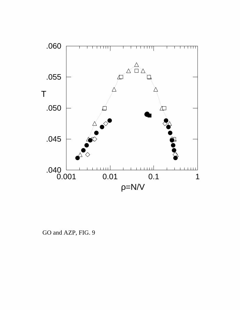
The coexistence curve of the restricted primitive model from the present work is shown in
Fig. 9. Our data do not extend much below the critical temperature due to difficulties associated
with sampling for the ionic fluids. The new coexistence data are compared with the earlier
results of Panagiotopoulos18, Caillol19 and Orkoulas and Panagiotopoulos20 that were obtained
from Gibbs ensemble simulations. While the agreement is reasonable for the subcritical
coexistence region, the previous Gibbs ensemble studies overestimate the critical temperature by
approximately 10%. This discrepancy can probably be attributed to analytic extensions of the
coexistence curve associated with finite systems and supercritical temperatures. These
extensions were falsely taken as evidence of true phase coexistence in all these studies and

14
consequently the critical temperature was overestimated. Because of the asymmetry of the RPM
phase diagram and the resulting strong and negative slope of the coexistence curve diameter, an
overestimation of Tc also results in an underestimation of ρc. This explains the difference in
critical density between the present study and that of references18-20. The critical density of the
RPM is now estimated to be approximately four times lower than that of simple non-polar fluids.
The vapor pressure curve for the RPM is shown in Fig. 10. Pressures were obtained by
using as reference sufficiently low densities so that the system behaves as an ideal gas of dimers
(ρ≈10-4). At the temperatures of interest, the RPM does not behave as an ideal gas of single ions
until much lower densities, not probed in our simulations. The critical compressibility factor
obtained from our estimate of the critical pressure is Zc=0.024, an order of magnitude lower than
for the non-ionic fluids. The lowest value of Zc in a compilation of experimental data for
common gases and liquids63 is Zc=0.12 for HF, with most values for other fluids in the range
Zc=0.25 to 0.40.
VI. CONCLUSIONS
In this work, we have utilized histogram-based and finite-size scaling techniques to
investigate the coexistence region of pure fluids by grand canonical Monte Carlo simulations.
These methodologies appear to provide a simple and highly efficient route to phase coexistence
calculations. The choice of the grand canonical ensemble was dictated by reasons of
computational simplicity. Similar results could, in principle, be obtained through constant
pressure (isothermal-isobaric) simulations. In such a case the density fluctuates by virtue of
volume expansions and compressions and the reweighting procedure can be applied by recording
histograms of molar volume. In addition, mixed-field finite size scaling techniques can also be
applied to fluids at constant pressure conditions.64 Constant pressure simulations might be
efficient for systems for which their pair potential functions scale with the box length. For most
fluids, however, trial volume moves are computationally expensive since they require a full
energy recalculation, an O(N2) operation. On the other hand, trial particle transfers in the grand
canonical ensemble are not too demanding since the associated energy change constitutes an
O(N) calculation.
It was confirmed from the finite-size scaling analysis that the critical points of the square-
well fluids with finite interaction range are of the Ising type. However, certain crossover effects

15
in the shape of the coexistence curve are apparent (Fig. 4). The interaction range must, of
course, play a significant role in the shape of the coexistence curve away from the critical point.
The critical compressibility factor was found to increase with the interaction range in accord with
theory.
In the absence of certainty about the nature of ionic criticality, we assumed that the
primitive model of electrolytes also belongs to the Ising universality class. Our data are
consistent with this hypothesis, but are not of sufficiently high accuracy and for a large enough
range of system sizes to exclude other possibilities. Similar conclusions were reached by Caillol
et al.59 in their study of the primitive model on a hypersphere. On the other hand, recent
simulation results by Valleau and Torrie65 provide no indication of an Ising-type divergence of
the heat capacity. Recent theoretical advances based on implementing the Ginzburg criterion66
for the restricted primitive model have found67,68,69,70 that this model should exhibit little (if any)
non-Ising behavior. Clearly, this latest picture that neither supports mean-field behavior nor a
crossover scenario contradicts several experimental observations. It is believed that charge
oscillations may provide a second order parameter that competes with the density fluctuations69.
This issue certainly deserves further theoretical and numerical study.
The critical temperature of the RPM was found to be Tc=0.0490±0.0003, lower than most
previous investigations. Due to the slope of the coexistence curve diameter, the new, lower
estimate for critical temperature also resulted in a significantly higher estimate for the critical
density. The critical compressibility factor, Zc=Pc/ρcTc, for the RPM is Zc=0.024±0.004, an
order of magnitude lower than non-ionic fluids. The low value of the critical compressibility
factor may serve as an indicator of true Coulombic criticality in experimental systems.
ACKNOWLEDGMENTS
The authors would like to thank Dr. N. B. Wilding for helpful discussions and for
providing copies of papers prior to publication, and Prof. M. E. Fisher for detailed comments on
a draft of the manuscript. GO would like to acknowledge the hospitality of Prof. D. N.
Theodorou at the University of Patras, Greece, where this manuscript was prepared. Financial
support for this work was provided by the Department of Energy, Office of Basic Energy
Sciences, under contract DE-FG02-89ER141014. Supercomputing time was provided by the
Cornell Theory Center.

16
REFERENCES
1 A. Z. Panagiotopoulos, Molec. Phys. 61, 813 (1987); Molecular Simulation 9, 1 (1992).
2 J. P. Valleau, J. Comp. Phys. 96, 193 (1991).
3 D. A. Kofke, Molec. Phys. 78, 1331 (1993); J. Chem. Phys. 98, 4149 (1993).
4 A. Lotfi, J. Vrabec, and J. Fischer, Molec. Phys., 76, 1319 (1992).
5 A. M. Ferrenberg and R. H. Swendsen, Phys. Rev. Lett. 61, 2635 (1988).
6 Finite Size Scaling and Numerical Simulation of Statistical Systems, edited by V. Privman
(World Scientific, Singapore, 1990).
7 A. M. Ferrenberg, and D. P. Landau, Phys. Rev. B 44, 5081 (1991).
8 K. Binder, in Computational Methods in Field Theory, edited by H. Gausterer and C. B. Lang
(Springer-Verlag, Berlin, 1992), pp. 59-125.
9 A. L. Talapov, and H. W. J. Blöte, J. Phys. A 29, 5727 (1996).
10A. D. Bruce and N. B. Wilding, Phys. Rev. Lett. 68, 193 (1992); N. B. Wilding and A. D.
Bruce, J. Phys. Condens. Matter 4, 3087 (1992).
11 A. Rotenberg, J. Chem. Phys. 43, 1198 (1965); D. Levesque, Physica 32, 1985 (1966); B. J.
Alder, D. A. Young, and M. A. Mark, J. Chem. Phys. 56, 3013 (1972); I. B. Schrodt and K.
D. Luks, ibid. 57, 200 (1972).
12 J. A. Barker and D. Henderson, Rev. Mod. Phys. 48, 587 (1976); D. Henderson, W. G.
Madden, and D. D. Fitts, J. Chem. Phys. 64, 5026 (1976); W. R. Smith and D. Henderson, J.
Chem. Phys. 69, 319 (1978); D. Henderson, O. H. Scalice, and W. R. Smith, ibid. 72, 2431
(1980).
13 G. A. Chapela, S. E. Martinez-Casas, and C. Varea, ibid., 86, 5683 (1987).
14 L. Vega, E. de Miguel, L. F. Rull, G. Jackson, and I. A. McLure, J. Chem. Phys. 96, 2296
(1992).15 A. L. Benavides, J. Alejandre, and F. Del Rio, Molec. Phys. 74, 321 (1991).

17
16 G. Stell, K. C. Wu, and B. Larsen, Phys. Rev. Lett. 27, 1369 (1976); M. Rovere, R. Miniero,
M. Parrinello, and M. P. Tosi, Phys. Chem. Liq. 9, 11 (1979); H. L. Friedman and B. Larsen,
J. Chem. Phys. 70, 92 (1979); W. Ebeling and M. Grigo, Ann. Physik. (Leipzig) 37, 21
(1980).
17 P. N. Vorontsov-Vel’yaminov and V. P. Chasovskikh, High Temp. (USSR) 13, 1071 (1975);
M. J. Gillan, Molec. Phys. 49, 421 (1983); K. S. Pitzer and D. R. Schreiber, ibid 60, 1067
(1987); J. P. Valleau, J. Chem. Phys. 95, 584 (1991).
18 A. Z. Panagiotopoulos, Fluid Phase Equilib. 76, 97 (1992).
19 J. M. Caillol, J. Chem. Phys. 102, 100 (1994).
20 G. Orkoulas and A. Z. Panagiotopoulos, J. Chem. Phys. 101, 1452 (1994).
21 M. E. Fisher and Y. Levin, Phys. Rev. Lett. 71, 3826 (1993); M. E. Fisher, J. Stat. Phys. 75, 1
(1994); X. Li, Y. Levin, and M. E. Fisher, Europhys. Lett. 26, 683 (1994); M. E. Fisher, Y.
Levin, and X. Li, J. Chem. Phys. 101, 2273 (1994); Y. Levin and M. E. Fisher, Physica A
225, 164 (1996).
22 G. Stell, J. Stat. Phys. 78, 197 (1995); Y. Zhou, S. Yeh, and G. Stell, J. Chem. Phys. 102,
5785 (1995); S. Yeh, Y. Zhou, and G. Stell, J. Phys. Chem. 100, 1415 (1995).
23 K. S. Pitzer, Acc. Che. Res. 23, 333 (1990); J. M. H. Levelt-Sengers and J. A. Given, Molec.
Phys. 80, 899 (1993).
24 M. L. Japas and J. M. H. Levelt-Sengers, J. Phys. Chem. 94, 5361 (1990).
25 S. Wiegand, M. Kleemeier, J. M. Schröder, W. Schröer, and H. Weingärtner, Int. J. Thermo.
15, 1045 (1994).
26 K. S. Pitzer, M. C. P. de Lima, and D. R. Schreiber, J. Phys. Chem. 89, 1854 (1985); R. R.
Singh and K. S. Pitzer, J. Am. Chem. Soc. 110, 8723 (1988); J. Chem Phys. 92, 6775 (1990).
27 K. C. Zang, M. E. Briggs, R. W. Gammon, and J. M. H. Levelt Sengers, J. Chem. Phys. 97,
8692 (1992).
28 P. Chieux, and M. J. Sienko, J. Chem. Phys. 53, 566 (1970).
18
29 T. Narayanan, and K. S. Pitzer, Phys. Rev. Lett. 73, 3002 (1994); J. Phys. Chem. 98, 9170
(1994); J. Chem. Phys. 102, 8118 (1995).
30 W. Schröer, M. Kleemeier, M. Plikat, V. Weiss, and S. Wiegand, J. Phys.: Condens. Matter 8,
9312 (1996).
31 S. Wiegand, J. M. H. Levelt Sengers, K. J. Zhang, M. E. Briggs, and R. W. Gammon, J. Chem.
Phys. 106, 2777 (1997).
32 Z. W. Salsburg, J. D. Jacobson, W. Fickett, and W. W. Wood, J. Chem. Phys. 30, 65 (1959);
D. A. Chesnut and Z. W. Salsburg, ibid. 38, 2861 (1963); I. R. McDonald and K. Singer,
ibid. 47, 4766 (1967); J. P. Valleau, and D. N. Card, ibid. 57, 5457 (1972).
33 A. M. Ferrenberg and R. H. Swendsen, Phys. Rev. Lett. 63, 1195 (1989).
34 T. L. Hill, Thermodynamics of small systems, Parts I and II (Dover, New York, 1962).
35 W. W. Wood, J. Chem. Phys. 48, 415 (1968).
36 K. Binder, Z. Phys. B 43, 119 (1981).
37 B. A. Berg and T. Neuhaus, Phys. Lett. B 267, 249 (1991); Phys. Rev. Lett. 68, 9 (1992).
38 J. Lee, Phys. Rev. Lett. 71, 211 (1993).
39 A. P. Lyubartev, A. A. Martsinovski, S. V. Shevkunov, and P. N. Vorontsov-Vel’yaminov, J.
Chem. Phys. 96, 1776 (1992).
40 E. Marinari, and G. Parisi, Europhys. Lett. 19, 451 (1992).
41 A. E. Ferdinand, and M. E. Fisher, Phys. Rev. 185, 832 (1969); M. E. Fisher and M. N.
Barber, Phys. Rev. Lett. 28, 1516 (1972).
42 J. J. Rehr and D. N. Mermin, Phys. Rev. A 8, 472 (1973).
43 B. Widom and J. S. Rowlinson, J. Chem. Phys. 52, 1670 (1970).
44 D. N. Mermin, Phys. Rev. Lett. 26, 169 (1970); ibid. 26, 957 (1971); J. J. Rehr and N. D.
Mermin, Phys. Rev. A 7, 379 (1973).
45 S. Jüngst, B. Knuth, and F. Hensel, Phys. Rev. Lett. 55, 2160 (1985).

19
46 A. D. Bruce, J. Phys. C: Solid State Phys. 14, 3667 (1981).
47 Tc for the three-dimensional Ising model is not known exactly. However, numerical
calculations give Tc to a high accuracy, see references 7 and 9 for instance.
48 R. Hilfer, and N. B. Wilding, J. Phys. A 28, L281 (1995).
49 G. E. Norman, and V. S. Filinov, High Temp. (USSR) 7, 216 (1969).
50 N. B. Wilding, Phys. Rev. E 52, 602 (1995).
51 J. V. Sengers and J. N. H. Levelt-Sengers, Ann. Rev. Phys. Chem. 37, 189 (1986).
52 A. J. Liu, and M. E. Fisher, Physica A 156, 35 (1989).
53 C. Borgs and R. Kotecky, J. Stat. Phys. 61, 79 (1990); Phys. Rev. Lett. 68, 1734 (1992).
54 N. V. Brilliantov and J. P. Valleau, J. Chem. Phys. 108, 1115 (1998); ibid. 108, 1123 (1998).
55 E. Luijten, H. W. J. Blöte, and K. Binder, Phys. Rev. E 54, 4626 (1996).
56 M. A. Anisimov, A. A. Povodyrev, V. D. Kulikov, and J. V. Sengers, Phys. Rev. Lett. 75,
3146 (1995).
57 Y. B. Melnichenko, M. A. Anisimov, A. A. Povodyrev, G. D. Wignall, J. V. Sengers, and W.
A. Van Hook, Phys. Rev. Lett. 79, 5266 (1997).
58 S. W. De Leeuw, J. W. Perram, and E. R. Smith, Proc. R. Soc. London A 373, 27 (1980); ibid.
373, 57 (1980); D. M. Heyes, J. Chem. Phys. 74, 1924 (1981); D. J. Adams, ibid. 78, 1585
(1983).
59 J. M. Caillol, D. Levesque, and J. J. Weis, Phys. Rev. Lett. 77, 4039 (1996); J. Chem. Phys.
107, 1565 (1997).
60 J. M. Caillol, J. Chem. Phys.99, 8953 (1993).
61 M. N. Barber , in Phase Transitions and Critical Phenomena, edited by C. Domb and J. L.
Lebowitz (Academic, New York, 1983), Vol. 8, pp. 145-266.
62 M. Müller, and N. B. Wilding, Phys. Rev. E 51, 2079 (1995).

20
63 R.C. Reid, J.M. Prausnitz and T.K. Sherwood, “The Properties of Gases and Liquids,” 3d
edition (McGraw-Hill, New York 1977).
64 N. B. Wilding and K. Binder, Physica A 231, 439 (1996).
65 J. Valleau, and G. Torrie, J. Chem. Phys. 108, 5169 (1998).
66 V. L. Ginzburg, Sov. Phys. Solid State 2, 1824 (1960).
67 R. J. F. Leote de Carvalho, and R. Evans, J. Phys. Condens. Matter 7, 575 (1995).
68 M. E. Fisher, J. Phys. Condens. Matter 8, 9103 (1996).
69 B. P. Lee, and M. E. Fisher, Phys. Rev. Lett 76, 2906 (1996); Europhys. Lett. 39, 611 (1997).
70 M. E. Fisher, and B. P. Lee, Phys. Rev. Lett. 77, 3561 (1996).

20
TABLE I Critical point parameters at the limit of infinite system size for the fluids studied
in this work. All quantities are made dimensionless as discussed in section II. Statistical
uncertainties are shown in parentheses, in units of the last decimal point reported for the
corresponding quantity. The value of r was obtained from the limiting slope of the coexistence
curve in the µ-K plane.
Fluid Tc ρc Pccc
cc T
PZ
ρ= µc/Tc s r
SW (λ=1.5) 1.2180(2) 0.310(1) 0.095(1) 0.252(3) -2.9576(2) -0.025(4) -4.8(2)
SW (λ=3) 9.87(1) 0.257(1) 0.84(1) 0.332(4) -2.8464(3) -0.005(1) -29.2(1)
RPM 0.0490(3) 0.070(5) 8.2(3)⋅10-5 0.024(4) -27.27(1) -1.5(1) -0.62(2)
FIGURE CAPTIONS
FIG. 1 Order parameter probability distribution PL(x) for the λ=1.5 square-well fluid. The
data have been obtained for an L=8 system size at T=1.220, and µ=-2.9518. The solid line
corresponds to the universal Ising distribution P*M(x), where x=ALβ/νδM. The nonuniversal scale
factor A has been chosen so that the distributions have unit variance.
FIG. 2 Critical temperature (a) and density (b) scaling with system size for the square-well
fluid with λ=3. Solid lines represent a least squares fit to the data.
FIG. 3 Coexistence curve of the square-well fluid with λ=1.5. Open symbols represent
grand canonical Monte Carlo results of this work. (Ο): L=6; (◊): L=8; (∆): L=12; (�): L=15.
(●): critical point estimate of this work. (■): Vega et al. (1992), Gibbs ensemble Monte Carlo.
Statistical uncertainties of the results from this work do not exceed the symbol sizes.

21
FIG. 4 Coexistence curve of the square-well fluid with λ=3. Open symbols represent grand
canonical Monte Carlo results of this work. (Ο): L=6; (◊): L=8; (∆): L=12; (�): L=15. (●):
critical point estimate of this work. (■): Benavides et al. (1991), molecular dynamics.
FIG. 5 Temperature dependence of the vapor pressure for the λ=1.5 square-well fluid. (Ο):
this work. (■): Brilliantov and Valleau, (1998). Simulation uncertainties are smaller than the
symbol size.
FIG. 6 Temperature dependence of the vapor pressure for the λ=3 square-well fluid.
Simulation uncertainties are smaller than the symbol size.
FIG. 7 Order parameter probability distribution for the restricted primitive model. (Ο):
L=14, T=0.05024, µ=-26.513. (): P*M(x).
FIG. 8 Critical temperature (a) and density (b) scaling scaling with system size for the
restricted primitive model. (Ο): this work. (�): Caillol et al. (1997).
FIG. 9 Coexistence curve for the restricted primitive model. (●): grand canonical Monte
Carlo results of this work. (■): critical point estimate of Caillol et al. (1997). (�):
Panagiotopoulos (1992). (∆): Caillol (1993). (◊): Orkoulas and Panagiotopoulos (1994).
FIG. 10 Temperature dependence of the vapor pressure for the restricted primitive model.
Statistical uncertainties are visible only for the critical pressure. For the other points, statistical
uncertainties are smaller than the symbol size. The larger uncertainties for Pc result from the
uncertainty in Tc.

GO and AZP FIG. 1
−3 −2 −1 0 1 2 3x = A L
β/ν δM
0.0
0.1
0.2
0.3
0.4
0.5
PL(x)

GO and AZP, FIG. 2
0 0.02 0.04 0.06L
−(1−α)/ν
.256
.258
.260
.262
0 0.002 0.004 0.006L
−(θ+1)/ν
9.6
9.7
9.8
9.9(a)
(b)
Tc(L)
ρc(L)

GO and AZP, FIG. 3
0 .1 .2 .3 .4 .5 .6 .7ρ=N/V
0.9
1.0
1.1
1.2
T

GO and AZP, FIG. 4
0 .1 .2 .3 .4 .5 .6ρ=N/V
7
8
9
10
T

GO and AZP, FIG. 5
0.9 1.0 1.1 1.2T
0.02
0.04
0.06
0.08
0.10
P

7 8 9 10T
0.2
0.4
0.6
0.8
P
GO and AZP, FIG. 6

GO and AZP, FIG. 7
−3 −2 −1 0 1 2 3x = AL
β/νδM
0.0
0.1
0.2
0.3
0.4
0.5
PL(x)

GO and AZP, FIG. 8
0 .01 .02 .03 .04L
−(1−α)/ν
.06
.07
.08
.09
0 .001 .002 .003 .004L
−(θ+1)/ν
.048
.049
.050
.051
.052
(a)
(b)
Tc(L)
ρc(L)
GO and AZP, FIG. 9
0.001 0.01 0.1 1ρ=N/V
.040
.045
.050
.055
.060
T

.042 .044 .046 .048 .050T
2
4
6
8
105P
GO and AZP, FIG. 10
Top Related