


Languages
Pages
Legal

An Introduction to Matched Asymptotic Expansions(A Draft)
Peicheng Zhu
Basque Center for Applied Mathematics andIkerbasque Foundation for Science
Nov., 2009
Preface
The Basque Center for Applied Mathematics (BCAM) is a newly foundedinstitute which is one of the Basque Excellence Research Centers (BERC).BCAM hosts a series of training courses on advanced aspects of applied andcomputational mathematics that are delivered, in English, mainly to graduatestudents and postdoctoral researchers, who are in or from out of BCAM. Theseries starts in October 2009 and finishes in June 2010. Each of the 13 coursesis taught in one week, and has duration of 10 hours.
This is the lecture notes of the course on Asymptotic Analysis that I gaveat BCAM from Nov. 9 to Nov. 13, 2009, as the second of this series of BCAMcourses. Here I have added some preliminary materials. In this course, weintroduce some basic ideas in the theory of asymptotic analysis. Asymptoticanalysis is an important branch of applied mathematics and has a broad rangeof contents. Thus due to the time limitation, I concentrate mainly on themethod of matched asymptotic expansions. Firstly some simple examples,ranging from algebraic equations to partial differential equations, are discussedto give the reader a picture of the method of asymptotic expansions. Then weend with an application of this method to an optimal control problem, whichis concerned with vanishing viscosity method and alternating descent methodfor optimal control of scalar conservation laws in presence of non-interactingshocks.
Thanks go to the active listeners for their questions and discussions, fromwhich I have learnt many things. The empirical law that “the best way forlearning is through teaching” always works to me.
Peicheng ZhuBilbao, Spain
Jan., 2010
i

ii
Contents
Preface i
1 Introduction 1
2 Algebraic equations 7
2.1 Regular perturbation . . . . . . . . . . . . . . . . . . . . . . . . 7
2.2 Iterative method . . . . . . . . . . . . . . . . . . . . . . . . . . 10
2.3 Singular perturbation . . . . . . . . . . . . . . . . . . . . . . . . 11
2.3.1 Rescaling . . . . . . . . . . . . . . . . . . . . . . . . . . 12
2.4 Non-ingeral powers . . . . . . . . . . . . . . . . . . . . . . . . . 15
3 Ordinary differential equations 17
3.1 First order ODEs . . . . . . . . . . . . . . . . . . . . . . . . . . 18
3.1.1 Regular . . . . . . . . . . . . . . . . . . . . . . . . . . . 18
3.1.2 Singular . . . . . . . . . . . . . . . . . . . . . . . . . . . 20
3.1.2.1 Outer expansions . . . . . . . . . . . . . . . . . 21
3.1.2.2 Inner expansions . . . . . . . . . . . . . . . . . 22
3.1.2.3 Matched asymptotic expansions . . . . . . . . . 23
3.2 Second order ODEs and boundary layers . . . . . . . . . . . . . 27
3.2.1 Outer expansions . . . . . . . . . . . . . . . . . . . . . . 29
3.2.2 Inner expansions . . . . . . . . . . . . . . . . . . . . . . 30
3.2.2.1 Rescaling . . . . . . . . . . . . . . . . . . . . . 30
3.2.2.2 Partly determined inner expansions . . . . . . . 32
3.2.3 Matching conditions . . . . . . . . . . . . . . . . . . . . 33
3.2.3.1 Matching by expansions . . . . . . . . . . . . . 33
3.2.3.2 Van Dyke’s rule for matching . . . . . . . . . . 34
3.2.4 Examples that the matching condition does not exist . . 37
3.2.5 Matched asymptotic expansions . . . . . . . . . . . . . . 37
3.3 Examples . . . . . . . . . . . . . . . . . . . . . . . . . . . . . . 38
iii
iv CONTENTS
4 Partial differential equations 414.1 Regular problem . . . . . . . . . . . . . . . . . . . . . . . . . . 414.2 Conservation laws and vanishing viscosity method . . . . . . . . 42
4.2.1 Construction of approximate solutions . . . . . . . . . . 434.2.1.1 Outer and inner expansions . . . . . . . . . . . 434.2.1.2 Matching conditions and approximations . . . . 44
4.2.2 Convergence . . . . . . . . . . . . . . . . . . . . . . . . . 454.3 Convergence of the approximate solutions . . . . . . . . . . . . 45
4.3.1 The equations are satisfied asymptotically . . . . . . . . 464.3.2 Proof of the convergence . . . . . . . . . . . . . . . . . . 52
5 An application to optimal control theory 575.1 Introduction . . . . . . . . . . . . . . . . . . . . . . . . . . . . . 575.2 Sensitivity analysis: the inviscid case . . . . . . . . . . . . . . . 62
5.2.1 Linearization of the inviscid equation . . . . . . . . . . . 625.2.2 Sensitivity in presence of shocks . . . . . . . . . . . . . . 655.2.3 The method of alternating descent directions: Inviscid
case . . . . . . . . . . . . . . . . . . . . . . . . . . . . . 675.3 Matched asymptotic expansions and approximate solutions . . . 72
5.3.1 Outer expansions . . . . . . . . . . . . . . . . . . . . . . 735.3.2 Derivation of the interface equations . . . . . . . . . . . 785.3.3 Inner expansions . . . . . . . . . . . . . . . . . . . . . . 815.3.4 Approximate solutions . . . . . . . . . . . . . . . . . . . 84
5.4 Convergence of the approximate solutions . . . . . . . . . . . . 865.4.1 The equations are satisfied asymptotically . . . . . . . . 875.4.2 Proof of the convergence . . . . . . . . . . . . . . . . . . 93
5.5 The method of alternating descent directions: Viscous case . . . 100Appendix . . . . . . . . . . . . . . . . . . . . . . . . . . . . . . . . . 104
Bibliography 107
Index 110
Chapter 1
Introduction
In the real world, many problems (which arise in applied mathematics, physics,engineering sciences, · · · , also pure mathematics like the theory of numbers)don’t have a solution which can be written a simple, exact, explicit formula.Some of them have a complex formula, but we don’t know too much aboutsuch a formula.
We now consider some examples. i) The Stirling formula:
n! ∼√2nπe−nnn
(1 +O
(1
n
)). (1.0.1)
The Landau symbol the big “O” and the Du Bois Reymond symbol “∼” areused. Note that n! grows very quickly as n → ∞ and becomes so large thatone can not have any idea about how big it is. But formula (1.0.1) gives us agood estimate of n!.
ii) From Algebra we know that in general there is no explicit solution toan algebraic equation with degree n ≥ 5.
iii) Most of problems in the theory of nonlinear ordinary or partial diffe-rential equations don’t have an exact solution.
And many others.
Why asymptotic? In practice, however, an approximation of a solution tosuch problems is usually enough. Thus the approaches to finding such an ap-proximation is important. There are two main methods. One is numericalapproximation, which is especially powerful after the invention of the compu-ter and is now regarded as the third most import method for scientific research(just after the traditional two: theoretical and experimental methods). Ano-ther is analytical approximation with an error which is understandable andcontrollable, in particular, the error could be made smaller by some rational
1
2 CHAPTER 1. INTRODUCTION
procedure. The term “analytical approximate solution” means that an ana-lytic formula of an approximate solution is found and its difference with theexact solution.
What is asymptotic? Asymptotic analysis is powerful tool for finding ana-lytical approximate solutions to complicated practical problems, which is animportant branch of applied mathematics. In 1886 the establishment of rigo-rous foundation was done by Poincare and Stieltjes. They published separatelypapers on asymptotic series. Later in 1905, Prandtl published a paper on themotion of a fluid or gas with small viscosity along a body. In the case ofan airfoil moving through air, such problem is described by the Navier-Stokesequations with large Reynolds number. The method of singular perturbationwas proposed.
History. Of course, the history of asymptotic analysis can be traced backto much earlier than 1886, even to the time when our ancestors studied theproblem, as small as the measure of a rod, or as large as the study of theperturbed orbit of a planet. As we know, when we measure a rod, each measuregives a different value, so n-measures result in n-different values. Which oneshould choose to be the length of this rod? The best approximation to thereal length of the rod is the mean value of these n-numbers, and each of themeasures can be regarded as a perturbation of the mean value.
The Sun’s gravitational attraction is the main force acting on each planet,but there are much weaker gravitational forces between the planets, whichproduce perturbations of their elliptical orbits; these make small changes ina planet’s orbital elements with time. The planets which perturb the Earth’sorbit most are Venus, Jupiter, and Saturn. These planets and the sun alsoperturb the Moon’s orbit around the Earth-Moon system’s center of mass.The use of mathematical series for the orbital elements as functions of timecan accurately describe perturbations of the orbits of solar system bodies forlimited time intervals. For longer intervals, the series must be recalculated.
Today, astronomers use high-speed computers to figure orbits in multiplebody systems such as the solar system. The computers can be programmedto make allowances for the important perturbations on all the orbits of themember bodies. Such calculations have now been made for the Sun and themajor planets over time intervals of up to several tens of millions of years.
As accurately as these calculations can be made, however, the behavior ofcelestial bodies over long periods of time cannot always be determined. Forexample, the perturbation method has so far been unable to determine thestability either of the orbits of individual bodies or of the solar system as awhole for the estimated age of the solar system. Studies of the evolution of
3
the Earth-Moon system indicate that the Moon’s orbit may become unstable,which will make it possible for the Moon to escape into an independent orbitaround the Sun. Recent astronomers have also used the theory of chaos toexplain irregular orbits.
The orbits of artificial satellites of the Earth or other bodies with atmos-pheres whose orbits come close to their surfaces are very complicated. Theorbits of these satellites are influenced by atmospheric drag, which tends tobring the satellite down into the lower atmosphere, where it is either vaporizedby atmospheric friction or falls to the planet’s surface. In addition, the shapeof Earth and many other bodies is not perfectly spherical. The bulge thatforms at the equator, due to the planet’s spinning motion, causes a strongergravitational attraction. When the satellite passes by the equator, it may beslowed enough to pull it to earth.
The above argument tells us that there are many problems with smallperturbations, some of those perturbations can be omitted under suitable as-sumptions. For instance, we are definitely allowed to omit their influence, onthe orbit of Earth around the Sun, of the gravity from some celestial bodieswhich are so distant from Earth that they can not be observed, or an artificialsatellite.
Main contents. The main contents of asymptotic analysis cover: perturba-tion method, the method of multi-scale expansions, averaging method, WKBJ(Wentzel, Kramers, Brillouin and Jeffreys) approximation, the method of mat-ched asymptotic expansions, asymptotic expansion of integrals, and so on.Thus due to the time limitation, this course is mainly concerned with themethod of matched asymptotic expansions. Firstly we study some simpleexamples arising in algebraic equation, ordinary differential equations, fromwhich we will get key ideas of matched asymptotic expansions, though thoseexamples are simple. Then we shall investigate matched asymptotic expansionsfor partial differential equations and finally take an optimal control problemas an application of the method of asymptotic expansions.
Let us now introduce some notations. D ⊂ Rd with d ∈ N denotes an opensubset in Rd. f, g, h : D → R are real continuous functions. We denote a smallquantity by ε.
The Landau symbols the big O and the little o, and the Du Bois Reymondsymbol “∼” will be used.
Definition 1.0.1 (asymptotic sequence) A sequence of gauge functions φn(x),n = 0, 1, 2, · · · , is said to be form an asymptotic sequence as x→ x0 if, for alln,
φn+1(x) = o(φn(x)), as x→ x0.
4 CHAPTER 1. INTRODUCTION
Definition 1.0.2 (asymptotic expansion) If φn(x) is an asymptotic sequenceof gauge functions as x→ x0, we say that
∞∑n=1
anφn(x), an are constant function,
is an asymptotic expansion (or an asymptotic approximation, or an asymptoticrepresentation) of a function f(x) as x→ x0, if for each N .
f(x) =N∑
n=1
anφn(x) + o(φN(x)), as x→ x0.
Note that, the last equation means that the remainder is smaller than thelast term included once the difference x− x0 is sufficiently small.
For various problems, their solution can be written as f = f(x; ε) where εis usually a small parameter. Suppose that we have the expansion
f(x; ε) ∼N∑
n=1
an(x)δn(ε), as ε→ 0.
If the approximation is asymptotic as ε → 0 for each fixed x, then it is calledvariously a Poincare, classical or straightforward asymptotic approximation.
If a function possesses an asymptotic approximation(expansion) in terms ofan asymptotic sequence, then that approximation is unique for that particularsequence.
Note that the uniqueness is for one given asymptotic sequence. Therefore, asingle function can have many asymptotic expansions, each in terms of differentasymptotic sequence. For instance,
tan(ε) ∼ ε+1
3ε3 +
2
15ε5
∼ sin(ε) +1
2(sin(ε))3 +
3
8(sin(ε))5
∼ ε cosh
(√2
3ε
)+
31
270
(cosh
(√2
3ε
))5
.
We also should note that the uniqueness is for one given function. Thusmany different functions may share the same asymptotic expansions, becausethey can differ by a quantity smaller than the last term included. For example,as ε→ 0
ε ∼ ε; ε+ exp
(− 1
ε2
)∼ ε,
5
and ε→ 0+
exp(ε) ∼∞∑n=0
εn
n!,
exp (ε) + exp
(−1
ε
)∼
∞∑n=0
εn
n!.
Therefore, the quantities ε and exp(− 1
ε2
)are equal up to to any order of
ε, we can regard them as the same in the sense of asymptotic expansions. Soare exp(ε) and exp (ε) + exp
(−1
ε
).

6 CHAPTER 1. INTRODUCTION
Chapter 2
Algebraic equations
In this chapter we shall investigate some algebraic equations, which are veryhelpful for establishing a picture of asymptotic analysis in our mind, thoughthose examples are quite simple. Let us consider algebraic equations with asmall positive parameter which is denoted by ε in what follows.
2.1 Regular perturbation
Consider firstly the following quadratic equation
x2 − εx− 1 = 0. (2.1.1)
Suppose that ε = 0, equation (2.1.1) becomes
x2 − 1 = 0. (2.1.2)
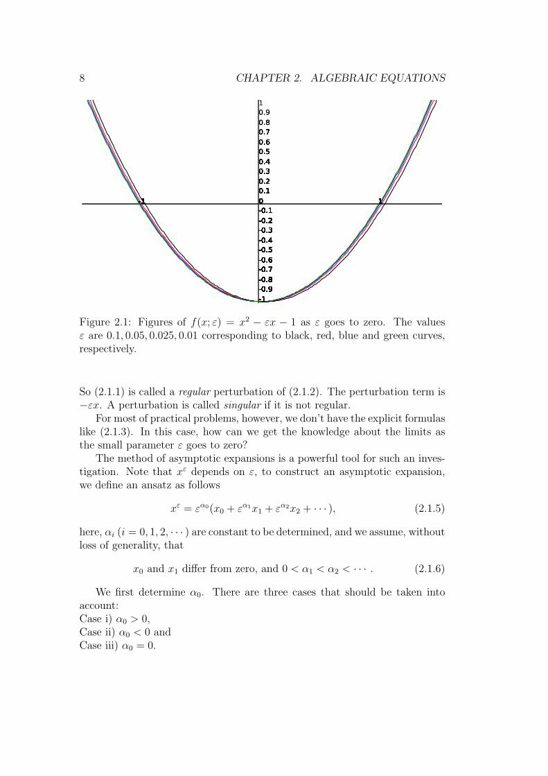
From Figure 2.1 we find that the roots of f(x; ε) converges to −1 and 1 respec-tively, and the curves become more and more similar rapidly, as ε → 0. Theblue curve with ε = 0.025 almost coincides with the green one correspondingto ε = 0.01.
In fact, it is easy to find the roots xε of (2.1.1), for any fixed ε, which read
xε1 =ε+
√ε2 + 4
2, and xε2 =
ε−√ε2 + 4
2. (2.1.3)
Correspondingly, the roots x0 of (2.1.2) are x01,2 = ±1.A natural question arises: Does xε converge to x0? With the help of formula
(2.1.3), we prove easily that
xε1 → x01, and xε2 → x02. (2.1.4)
7
8 CHAPTER 2. ALGEBRAIC EQUATIONS
Figure 2.1: Figures of f(x; ε) = x2 − εx − 1 as ε goes to zero. The valuesε are 0.1, 0.05, 0.025, 0.01 corresponding to black, red, blue and green curves,respectively.
So (2.1.1) is called a regular perturbation of (2.1.2). The perturbation term is−εx. A perturbation is called singular if it is not regular.
For most of practical problems, however, we don’t have the explicit formulaslike (2.1.3). In this case, how can we get the knowledge about the limits asthe small parameter ε goes to zero?
The method of asymptotic expansions is a powerful tool for such an inves-tigation. Note that xε depends on ε, to construct an asymptotic expansion,we define an ansatz as follows
xε = εα0(x0 + εα1x1 + εα2x2 + · · · ), (2.1.5)
here, αi (i = 0, 1, 2, · · · ) are constant to be determined, and we assume, withoutloss of generality, that
x0 and x1 differ from zero, and 0 < α1 < α2 < · · · . (2.1.6)
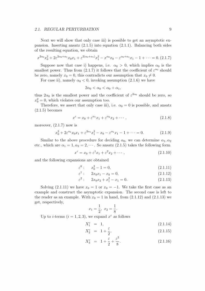
We first determine α0. There are three cases that should be taken intoaccount:Case i) α0 > 0,Case ii) α0 < 0 andCase iii) α0 = 0.
2.1. REGULAR PERTURBATION 9
Next we will show that only case iii) is possible to get an asymptotic ex-pansion. Inserting ansatz (2.1.5) into equation (2.1.1). Balancing both sidesof the resulting equation, we obtain
x2α0x20 + 2ε2α0+α1x0x1 + ε2(α0+α1)x21 − xα0x0 − εα0+α1x1 − 1 + · · · = 0. (2.1.7)
Suppose now that case i) happens, i.e. α0 > 0, which implies α0 is thesmallest power. Thus from (2.1.7) it follows that the coefficient of εα0 shouldbe zero, namely x0 = 0, this contradicts our assumption that x0 = 0.
For case ii), namely α0 < 0, invoking assumption (2.1.6) we have
2α0 < α0 < α0 + α1,
thus 2α0 is the smallest power and the coefficient of ε2α0 should be zero, sox20 = 0, which violates our assumption too.
Therefore, we assert that only case iii), i.e. α0 = 0 is possible, and ansatz(2.1.5) becomes
xε = x0 + εα1x1 + εα2x2 + · · · , (2.1.8)
moreover, (2.1.7) now is
x20 + 2εα1x0x1 + ε2α1x21 − x0 − εα1x1 − 1 + · · · = 0. (2.1.9)
Similar to the above procedure for deciding α0, we can determine α1, α2
etc., which are α1 = 1, α2 = 2, · · · . So ansatz (2.1.5) takes the following form
xε = x0 + ε1x1 + ε2x2 + · · · , (2.1.10)
and the following expansions are obtained
ε0 : x20 − 1 = 0, (2.1.11)
ε1 : 2x0x1 − x0 = 0, (2.1.12)
ε2 : 2x0x2 + x21 − x1 = 0. (2.1.13)
Solving (2.1.11) we have x0 = 1 or x0 = −1. We take the first case as anexample and construct the asymptotic expansion. The second case is left tothe reader as an example. With x0 = 1 in hand, from (2.1.12) and (2.1.13) weget, respectively,
x1 =1
2, x2 =
1
8.
Up to i-terms (i = 1, 2, 3), we expand xε as follows
Xε1 = 1, (2.1.14)
Xε2 = 1 +
ε
2, (2.1.15)
Xε3 = 1 +
ε
2+ε2
8. (2.1.16)
10 CHAPTER 2. ALGEBRAIC EQUATIONS
The next question then arise: How precisely does Xεi (i = 1, 2, 3) satisfy
the equation of xε?Straightforward computations yield that
(Xε1)
2 − εXε1 − 1 = O(ε), (2.1.17)
(Xε2)
2 − εXε2 − 1 = O(ε2), (2.1.18)
(Xε3)
2 − εXε3 − 1 = O(ε4). (2.1.19)
From which it is easy to see that Xεi satisfies very well the equation when ε is
small, and the error becomes smaller as i is larger, which means that we takemore terms.
This example illustrates how powerful the method of asymptotic expansionsis in finding an analytic approximation without a priori knowledge on thesolution to a problem under consideration.
2.2 Iterative method
In this section we are going to make use the so-called iterative method toconstruct asymptotic expansions again for equation (2.1.1). We rewrite (2.1.1)as
x = ±√1 + εx,
where x = xε. This formula suggests us an iterative procedure,
xn+1 =√1 + εxn (2.2.1)
for any n ∈ N. Here we only take the positive root as an example. Let x0 bea fixed real number. One then obtains from (2.2.1) that
x1 = 1 +ε
2x0 + · · · , (2.2.2)
so we find the first term of an asymptotic expansion, however the secondterm in (2.2.2) still depends on x0. To get the second term of an asymptoticexpansion, we iterate once again and arrive at
x2 = 1 +ε
2x1 + · · · = 1 +
ε
2+ · · · , (2.2.3)
this gives us the desired result. After iterating twice, we then construct anasymptotic expansion:
xε = 1 +ε
2+ · · · . (2.2.4)
2.3. SINGULAR PERTURBATION 11
Calculating the derivative of the function
x 7→ f(x) :=1√
1 + εx,
we have
|f ′(x)| =∣∣∣∣12 ε√
1 + εx
∣∣∣∣ ≤ ε
2,
from this it follows easily that the iteration defined by (2.2.1) converges, sinceε is a small number.
The shortage of this method for constructing an asymptotic expansion isthat we don’t have an explicit formula, like (2.2.1), which guarantees the ite-ration converges.
2.3 Singular perturbation
Now we start to investigate the following equation, which will give us verydifferent results, compared with the previous section.
εx2 − x− 1 = 0. (2.3.1)
Suppose that ε = 0, equation (2.3.1) becomes
−x− 1 = 0. (2.3.2)
Therefore we see that one root of (2.3.1) disappears as ε becomes 0. Thisis very different from (2.1.1). It is not difficult to get the roots of (2.3.1) whichread
xε =1±
√1 + 4ε
2ε.
There hold, as ε→ 0, that
xε− =1−
√1 + 4ε
2ε→ −1,
and by a Taylor expansion,
xε+ =1 +
√1 + 4ε
2ε
=1
2ε
(1 + 1 + 2ε− 2ε2 + · · ·
)=
1
ε+ 1− 2ε+ · · · . (2.3.3)
12 CHAPTER 2. ALGEBRAIC EQUATIONS
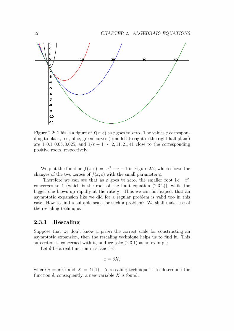
Figure 2.2: This is a figure of f(x; ε) as ε goes to zero. The values ε correspon-ding to black, red, blue, green curves (from left to right in the right half plane)are 1, 0.1, 0.05, 0.025, and 1/ε + 1 ∼ 2, 11, 21, 41 close to the correspondingpositive roots, respectively.
We plot the function f(x; ε) := εx2 − x− 1 in Figure 2.2, which shows thechanges of the two zeroes of f(x; ε) with the small parameter ε.
Therefore we can see that as ε goes to zero, the smaller root i.e. xε−converges to 1 (which is the root of the limit equation (2.3.2)), while thebigger one blows up rapidly at the rate 1
ε. Thus we can not expect that an
asymptotic expansion like we did for a regular problem is valid too in thiscase. How to find a suitable scale for such a problem? We shall make use ofthe rescaling technique.
2.3.1 Rescaling
Suppose that we don’t know a priori the correct scale for constructing anasymptotic expansion, then the rescaling technique helps us to find it. Thissubsection is concerned with it, and we take (2.3.1) as an example.
Let δ be a real function in ε, and let
x = δX,
where δ = δ(ε) and X = O(1). A rescaling technique is to determine thefunction δ, consequently, a new variable X is found.
2.3. SINGULAR PERTURBATION 13
Rewriting (2.3.1) in X, we have
εδ2X2 − δX − 1 = 0. (2.3.4)
By comparing the coefficients of (2.3.4), namely,
εδ2, δ, 1,
we divide the rescaling argument into five cases.
Case i) δ << 1. Then (2.3.4) can be written as
1 = εδ2X2︸ ︷︷ ︸o(1)
− δX︸︷︷︸o(1)
= o(1), (2.3.5)
which can not be true since the left hand side of (2.3.5) while the right handside is a very small quantity.
Case ii) δ = 1, which means there is no any change to (2.3.1). (2.3.4) becomes
εX2︸︷︷︸o(1)
−X − 1 = 0, (2.3.6)
thus it is impossible that X = 1 and we can construct a regular asymptoticexpansion but cannot recover the lost root.
Case iii) 1 << δ << 1εwhich implies that δε << 1. Dividing equation (2.3.4)
by δ we obtain
εδX2︸ ︷︷ ︸o(1)
−X − 1
δ︸︷︷︸o(1)
= 0, (2.3.7)
and X = o(1). This is impossible.
Case iv) δ = 1ε, namely δε = 1, also δ >> 1 since we assume that ε << 1.
Consequently, we infer from (2.3.4) that
X2 −X − 1
δ︸︷︷︸o(1)
= 0, (2.3.8)
Thus X ∼ 0 or 1. This gives us the correct scale.
Case v) δ >> 1ε, thus δε >> 1. Multiplying (2.3.4) by ε−1δ−2 yields
X2 − (εδ)−1X︸ ︷︷ ︸o(1)
− 1
εδ2︸︷︷︸o(1)
= 0, (2.3.9)
14 CHAPTER 2. ALGEBRAIC EQUATIONS
and X = o(1). So this is not a suitable scale either.
In conclusion, the suitable scale is δ = 1ε, thus
x =X
ε.
Equation (2.3.4) is changed to
X2 −X − ε = 0. (2.3.10)
A singular problem is reduced to a regular one.
We now turn back to equation (2.3.1). Rescaling suggests us to use thefollowing ansatz:
xε = ε−1x−1 + x0 + εx1 + · · · . (2.3.11)
Inserting into (2.3.1) and comparing the coefficients of ε1 (i = −1, 0, 1, · · · )on both sides of (2.3.1), we obtain
ε−1 : x2−1 − x−1 = 0, (2.3.12)
ε0 : 2x0x−1 − x0 − 1 = 0, (2.3.13)
ε1 : x20 + 2x−1x1 − x1 = 0. (2.3.14)
The roots of (2.3.12) are x−1 = 1 and x−1 = 0. The second root does not yielda singular asymptotic expansion, thus it can be excluded easily. We considernow x−1 = 1. From (2.3.13) and (2.3.14) one solves
x0 = 1, x1 = −1.
Therefore, we construct expansions Xεi , up to i + 1-terms(i = 0, 1, 2), of
the root xε+ by
Xε2 =
1
ε+ 1− ε, (2.3.15)
Xε1 =
1
ε+ 1, (2.3.16)
and
Xε0 =
1
ε. (2.3.17)
2.4. NON-INGERAL POWERS 15
How precisely do they satisfy equation (2.3.1)? Computations yield
ε(Xε0)
2 −Xε0 − 1 = −1,
correspondingly, xε+ − Xε0 = 1 − 2ε + o(ε) → 1 = 0. This means that an
expansion with one term is not a good approximation.
ε(Xε1)
2 −Xε1 − 1 = ε,
andε(Xε
2)2 −Xε
2 − 1 = O(ε2),
meanwhile, we have the following estimates
xε+ −Xε0 = O(1),
xε+ −Xε1 = O(ε),
xε+ −Xε2 = O(ε2).
Thus Xε1 , X
ε2 are a good approximation to xε+, however X
ε0 is not a good
one. Moreover, we can conclude that the more terms we take, the more precisethe approximation is. This is not always true as we shall see in Chapter 2,the example of ordinary differential equation of second order. We also figureout the profile approximately of xε+, in other word, we know now how the rootdisappears by blowing up as ε goes to zero.
2.4 Non-ingeral powers
Any of the asymptotic expansions in Sections 1.1 and 1.2 are a series withintegral powers. However this is in general not true. Here we give an example.Consider
(1− ε)x2 − 2x+ 1 = 0. (2.4.1)
Define, as in previous sections, an ansatz as follows
xε = x0 + εx1 + εx2 + · · · , (2.4.2)
inserting (2.4.2) into (2.4.1) and balancing both sides yield
ε0 : x20 − 2x0 + 1 = 0, (2.4.3)
ε0 : 2x0x1 − 2x1 − x20 = 0, (2.4.4)
ε1 : 2x0x2 − 2x2 + x21 − 2x0x1 = 0. (2.4.5)
16 CHAPTER 2. ALGEBRAIC EQUATIONS
From (2.4.3) one gets x0 = 1, whence (2.4.4) implies 2x1 − 2x1 − 12 = 0,that is 1 = 0, a contradiction. So (2.4.2) is not well-defined.
Now we define an ansatz as
xε = x0 + εαx1 + εβx2 + · · · , (2.4.6)
where 0 < α < β < · · · are constants to be determined. inserting this ansatzinto (2.4.1) and balancing both sides, we obtain there must hold that
α =1
2, β = 1, · · · .
and the correct ansatz is
xε = x0 + ε12x1 + εx2 + ε
32x3 + · · · . (2.4.7)
The remaining part of construction is similar to previous ones, just by intro-ducing simply η = ε
12 . We have
xε = 1± ε12 + ε± ε
32 + · · · .
Chapter 3
Ordinary differential equations
This chapter is concerned with the study of ordinary differential equation andwe start with some definitions. Consider
L0[u] + εL1[u] = f0 + εf1, in D. (3.0.1)
and the associated equation corresponding to the case that ε = 0
L0[u] = f0, in D. (3.0.2)
Here, L0, L1 are known operators, either ordinary or partial; f0, f1 are givenfunctions. The terms εL1[u] and εf1 are called perturbations.
Eε (E0, respectively) denotes the problem consisting equation (3.0.1) (equa-tion (3.0.2)) and suitable boundary/initial conditions. The solution to problemEε (E0, respectively) is denoted by uε (u0).
Definition 3.0.1 Problem Eε is regular if
∥uε − u0∥D → 0,
as ε → 0. Otherwise, Problem Eε is referred to a singular one. Here ∥ · ∥D isa suitable norm over domain D.
It is easy to expect that whether a problem is regular or not, this dependson the choice of the norm, which can be clarified by the following problem.
Example 3.0.1 Let D = (0, 1) and φ : D → R be a real function, which is asolution to
εd2φ
dx2+dφ
dx= 0, in D, (3.0.3)
φ|x=0 = 0,
φ|x=1 = 1. (3.0.4)
17
18 CHAPTER 3. ORDINARY DIFFERENTIAL EQUATIONS
The solution φ is
φ = φ(x; ε) =1− e−
xε
1− e−1ε
,
which is monotone increasing.
Now we define two norms. i) ∥φ∥D = maxD |φ|, then problem (3.0.3) –(3.0.4) is singular since ∥φ− φ0∥D = 1 where φ0 = 0 or φ0 = 1.
ii) Define
∥φ∥D =
(∫D
|φ|2) 1
2
,
choose φ0 = 1 which satisfies dφdx
= 0, then we can prove easily that ∥φ −φ0∥D → 0 as ε→ 0, whence problem (3.0.3) – (3.0.4) is regular.
In what follows, we restrict ourself to consider only themaximum norm, andin the remaining part of this chapter the domain D is defined by D = (0, 1).
3.1 First order ODEs
This section is devoted to discussion matched asymptotic expansions in thecontext of ordinary differential equations, and we will get new ideas which cannot be expected in the examples of algebraic equations since those are toosimple. Both regular and singular problems will be studied.
3.1.1 Regular
In this subsection we first study a regular problem of ordinary differentialequations of first order. Consider the following problem
du
dx+ u = εx, in D, (3.1.1)
u(0) = 1, (3.1.2)
and its associated problem
du
dx+ u = 0, in D, (3.1.3)
u(0) = 1. (3.1.4)
They are simple problems, however we shall see later that they give us almostall features of matched asymptotic expansions.
3.1. FIRST ORDER ODES 19
We can solve easily problems (3.1.1) – (3.1.2) and (3.1.3) – (3.1.4) whosesolution reads
uε(x) = (1 + ε)e−x + ε(x− 1), (3.1.5)
u0(x) = e−x. (3.1.6)
Calculating the difference of these two solutions yields
∥uε − u0∥D = εmaxD
|e−x + x− 1| → 0
as ε→ 0.Therefore, problem (3.1.1) – (3.1.4) is regular, and the term εx is a regular
perturbation.
But, in general, one can not expect that there are the explicit simple for-mulas, like (3.1.5) and (3.1.6), of exact solutions. Thus we next deal with thisproblem in a general way, and employ the method of asymptotic expansions.To this end, we define an ansatz
uε(x) = u0(x) + εu1(x) + ε2u2(x) + · · · . (3.1.7)
Then inserting it into equation (3.1.1) and comparing the coefficients of εi inboth sides of the resulting equation, we get
ε0 : u′0 + u0 = 0, (3.1.8)
ε0 : u′1 + u1 = x, (3.1.9)
ε1 : u′2 + u2 = 0. (3.1.10)
We need to derive the initial conditions for ui. The condition for u0 followsfrom (3.1.4) and ansatz (3.1.7). In fact, there holds
1 = uε(0) = u0(0) + εu1(0) + ε2u2(0) + · · · → u0(0), (3.1.11)
thus, u0(0) = 1. With this in hand, we use again (3.1.11) to derive the condi-tion for u1. We obtain
0 = εu1(0) + ε2u2(0) + · · · , whence0 = u1(0) + εu2(0) + · · · (3.1.12)
Letting ε → 0 we get u1(0) = 0. In a similar manner, we find the conditionfor u2. Thus the conditions should be met
u0(0) = 1, (3.1.13)
u1(0) = 0, (3.1.14)
u2(0) = 0. (3.1.15)
20 CHAPTER 3. ORDINARY DIFFERENTIAL EQUATIONS
Solving equations (3.1.8), (3.1.9) and (3.1.10) with conditions (3.1.13),(3.1.14) and (3.1.15), respectively, we obtain
u0(x) = e−x, (3.1.16)
u1(x) = x− 1 + e−x, (3.1.17)
u2(x) = 0. (3.1.18)
Thus the approximations can be constructed:
U ε0 (x) = e−x, (3.1.19)
U ε1 (x) = U ε
2 (x) (3.1.20)
= (1 + ε)e−x + ε(x− 1). (3.1.21)
Simple calculations show that U ε0 (x) satisfies (3.1.1) with a small error
(U ε0 (x))
′ + U ε0 (x)− εx = O(ε),
and condition (3.1.4) is satisfied exactly. Note that U ε1 (x) = U ε
2 (x) are equalto the exact solution (3.1.5), so they solve problem (3.1.1) – (3.1.4), and are aperfect “approximation”.
3.1.2 Singular
Now we are going to study singular perturbation and boundary layers. Theperturbed problem is
εdu
dx+ u = x, in D, (3.1.22)
u(0) = 1, (3.1.23)
and the associated one is
u(x) = x, in D, (3.1.24)
u(0) = 1, (3.1.25)
from which one can easily see the condition (3.1.25) can not be satisfied, thusa boundary layer happens at x = 0. The exact solutions of problem (3.1.22) –(3.1.23) is
uε(x) = (1 + ε)e−x + x− ε, (3.1.26)
Let u0(x) = x. Computation yields
∥uε − u0∥D = maxD
|(1 + ε)e−x − ε| = 1,
3.1. FIRST ORDER ODES 21
for any positive ε. Therefore, by definition, problem (3.1.22) – (3.1.23) issingular, and the term εdu
dxis a singular perturbation.
We next want to employ the method of asymptotic expansions to studythis singular problem, for such a problem at least one boundary layer arisesand a matched asymptotic expansion is suitable for it. We will constructouter and inner expansions which are valid (by this word we mean that anexpansion satisfies well the corresponding equation) in the so-called outer andinner regions, respectively. Then we derive matching conditions which areenable us to establish an asymptotic expansion which is valid uniformly in thewhole domain.
We now explain the regions in Figure 3.1, the boundary layer or innerregion occurs near x = 0, it is very thin, the O(ε) part, see Figure 3.1. Anouter region is the subset of (0, 1) consisting of the points far from the boundarylayer, which the O(1) part, the largest part and usually occupies most part ofthe domain under consideration. Therefore as ε increases to the size of O(1),the inner regime passes to the outer one, from this we see that there is anintermediate (or, matching, overlapping) region between them, the scale ofthis region is of O(εγ) where γ ∈ (0, 1), in the present problem. This region isvery large compared with the inner one, however is very small compared withthe outer one.
We now turn to the construction of asymptotic expansions, and start withouter expansions.
3.1.2.1 Outer expansions
The ansatz for deriving outer expansion is just of the form of a regular expan-sion:
uε(x) = u0(x) + εu1(x) + ε2u2(x) + · · · , (3.1.27)
Similar to the approach for asymptotic expansion of the regular problem(3.1.1) – (3.1.4), we obtain
ε0 : u0(x) = x, (3.1.28)
ε1 : u1(x) + u′0(x) = 0, (3.1.29)
ε2 : u2(x) + u′1(x) = 0. (3.1.30)
Solving the above problems yields
u0(x) = x, (3.1.31)
u1(x) = −1, (3.1.32)
u2(x) = 0. (3.1.33)
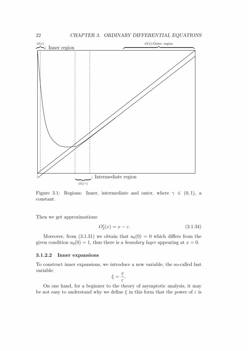
22 CHAPTER 3. ORDINARY DIFFERENTIAL EQUATIONS
O(ε)︷︸︸︷: Inner region O(1):Outer region︷ ︸︸ ︷
︸ ︷︷ ︸O(εγ)
: Intermediate region
Figure 3.1: Regions: Inner, intermediate and outer, where γ ∈ (0, 1), aconstant.
Then we get approximations:
Oε2(x) = x− ε. (3.1.34)
Moreover, from (3.1.31) we obtain that u0(0) = 0 which differs from thegiven condition u0(0) = 1, thus there is a boundary layer appearing at x = 0.
3.1.2.2 Inner expansions
To construct inner expansions, we introduce a new variable, the so-called fastvariable:
ξ =x
ε,
On one hand, for a beginner to the theory of asymptotic analysis, it maybe not easy to understand why we define ξ in this form that the power of ε is
3.1. FIRST ORDER ODES 23
1? To convince oneself, one may assume a more general form as ξ = xεα
withα ∈ R. Then repeating the procedure we will carry out later in next subsection,we prove that α must be equal to 1 in order to get an asymptotic expansion.On the other hand we already assume that a boundary layer occurs at x = 0.If the assumption is incorrect, the procedure will break down when you tryto match the inner and outer expansions in the intermediate region. At thispoint one may assume that there exists a boundary layer near a point x = x0.The following analysis is the same, except that the scale transformation in theboundary layer is ξ = x−x0
εδ. We shall carry out the analysis for determining δ
in the next section.An inner expansion is an expansion in terms of ξ, we assume that
uε(x) = U0(ξ) + εU1(ξ) + ε2U2(ξ) + · · · . (3.1.35)
It is easy to compute that for i = 0, 1, 2, · · · ,
dUi(ξ)
dx=
1
ε
dUi(ξ)
dξ.
Invoking equation (3.1.1) we arrive at
ε−1 : U ′0 + U0 = 0, (3.1.36)
ε0 : U ′1 + U1 = ξ, (3.1.37)
ε1 : U ′2 + U2 = 0. (3.1.38)
From which we have
U0(ξ) = C0e−ξ, (3.1.39)
U1(ξ) = C1e−ξ + ξ − 1, (3.1.40)
U2(ξ) = C2e−ξ. (3.1.41)
The second step is to determine the constants Ci with i = 0, 1, 2. To thisend, we use the condition at x = 0 which implies that ξ = 0 too to concludethat U0(0) = 1, thus C0 = 1. Similarly we have C1 = 1, C2 = 0. Therefore,an inner expansion can be obtained
Iε2(ξ) = (1 + ε)e−ξ + ε(ξ − 1). (3.1.42)
3.1.2.3 Matched asymptotic expansions
Here we shall discuss two main approaches to construct a uniform asymptoticexpansion by combining together the inner and outer expansions. The firstone is to take the sum of the inner expansion (3.1.42) and the outer expansion
24 CHAPTER 3. ORDINARY DIFFERENTIAL EQUATIONS
(3.1.34), then subtract their common part which is valid in the intermediateregion.
To get a matched asymptotic expansion, it remains to find the commonpart. Assume that there exists a uniform asymptotic expansion, say U ε
2 , thenthere holds
limx∈ outer region, x→0
U ε2 (x) = lim
x→0Oε
2(x) (3.1.43)
limx∈ inner region, x→0
U ε2 (x) = lim
x→0Iε2(
x
ε), (3.1.44)
thus, there must hold
U0(ξ) + εU1(ξ) + ε2U2(ξ) = u0(x) + εu1(x) + ε2u2(x) +O(ε3).
Following Fife [14], we rewrite x = εξ and expand the right hand side in termsof ξ. There hold
U0(ξ) + εU1(ξ) + ε2U2(ξ)
= u0(εξ) + εu1(εξ) + ε2u2(εξ) +O(ε3)
= u0(0) + u′0(0)εξ +1
2u′′0(0)(εξ)
2
+ε(u1(0) + u′1(0)εξ) + ε2u2(0) +O(ε3)
= u0(0) + ε(u′0(0)ξ + u1(0))
+ε2(1
2u′′0(0)ξ
2 + u′1(0)ξ) + u2(0)
)+O(ε3). (3.1.45)
Therefore we obtain the following matching conditions
U0(ξ) = u0(0) = 0, (3.1.46)
U1(ξ) ∼ u′0(0)ξ + u1(0) = ξ − 1, (3.1.47)
U2(ξ) ∼ 1
2u′′0(0)ξ
2 + u′1(0)ξ + u2(0) = 0, (3.1.48)
for ξ → ∞.The common parts, respectively, are
i) if we take the first one term
Common part0 = 0,
ii) if we take the first two terms,
Common part1 = ε(ξ − 1).

3.1. FIRST ORDER ODES 25
iii) if we take the first three terms,
Common part2 = ε(ξ − 1).
The matched asymptotic expansion then is
U ε2 (x) = Iε2(ξ) +Oε
2(x)− Common part2= (1 + ε)e−ξ + ε(ξ − 1) + (x− ε)− ε(ξ − 1)
= (1 + ε)e−ξ + x− ε. (3.1.49)
So U ε2 (x) is just the exact solution to problem (3.1.22) – (3.1.23). Similarly, we
also can construct an asymptotic expansion up to one, two terms which readrespectively,
U ε0 (x) = Iε0(ξ) +Oε
0(x)− Common part0 = e−ξ + x,
and
U ε1 (x) = Iε1(ξ) +Oε
1(x)− Common part1 = U ε2 (x).
We thus can draw the graphs (see Figure 3.2) of uε, u0, Oε2, U
ε2 and Iε2 , re-
membering that uε = U ε2 = Iε2 , one needs only to plot the first three functions.
The second method for constructing a matched asymptotic expansion frominner and outer expansions is to make use of a suitable cut-off function to forma linear combination of inner and outer expansions.
We define a function χ = χ(ξ) : R+ → R+ which is smooth such that
χ(ξ) =
1 if ξ ≤ 1,
0 if ξ ≥ 2,(3.1.50)
and 0 ≤ χ(ξ) ≤ 1 if ξ ∈ [1, 2]. And let
χε(x) = χ(ε−γx), (3.1.51)
which is easily seen that
supp(χε) ⊂ [0, 2εγ], supp(χ′ε) ⊂ [εγ, 2εγ].
Here γ ∈ (0, 1) is a fixed number. χε, χ′ε are plotted in 3.3.
Now we are able to define an approximation by
U ε2 (x) = (1− χε(x))O
ε2(x) + χε(x)I
ε2(x
ε). (3.1.52)
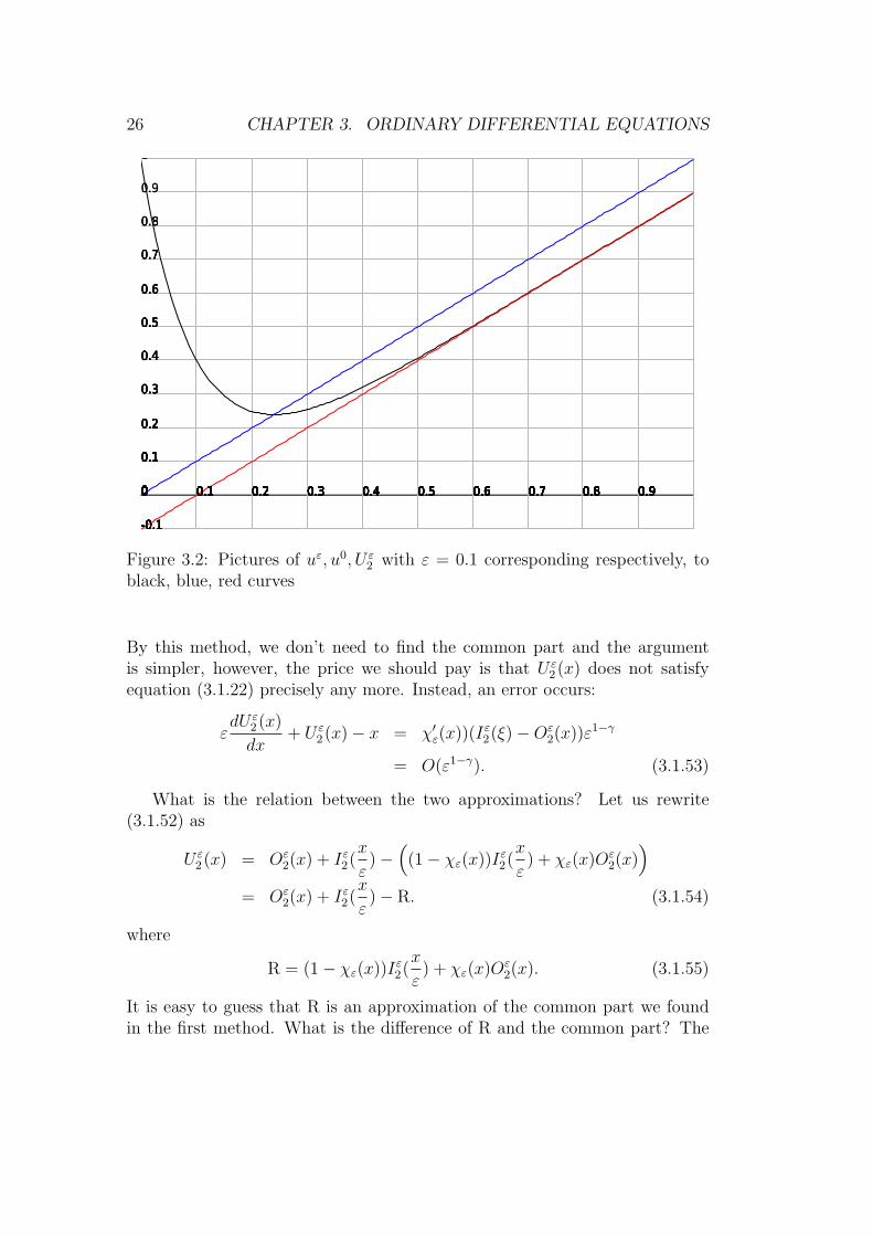
26 CHAPTER 3. ORDINARY DIFFERENTIAL EQUATIONS
Figure 3.2: Pictures of uε, u0, U ε2 with ε = 0.1 corresponding respectively, to
black, blue, red curves
By this method, we don’t need to find the common part and the argumentis simpler, however, the price we should pay is that U ε
2 (x) does not satisfyequation (3.1.22) precisely any more. Instead, an error occurs:
εdU ε
2 (x)
dx+ U ε
2 (x)− x = χ′ε(x))(I
ε2(ξ)−Oε
2(x))ε1−γ
= O(ε1−γ). (3.1.53)
What is the relation between the two approximations? Let us rewrite(3.1.52) as
U ε2 (x) = Oε
2(x) + Iε2(x
ε)−
((1− χε(x))I
ε2(x
ε) + χε(x)O
ε2(x)
)= Oε
2(x) + Iε2(x
ε)− R. (3.1.54)
where
R = (1− χε(x))Iε2(x
ε) + χε(x)O
ε2(x). (3.1.55)
It is easy to guess that R is an approximation of the common part we foundin the first method. What is the difference of R and the common part? The
3.2. SECOND ORDER ODES AND BOUNDARY LAYERS 27
O εγ 2εγ
1
χε(x)
x
χ′ε(x)
O 2εγ x
ε−γ
εγ
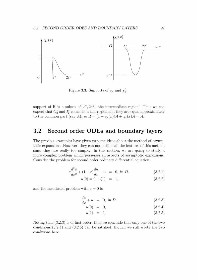
Figure 3.3: Supports of χε and χ′ε.
support of R is a subset of [εγ, 2εγ], the intermediate region! Thus we canexpect that Oε
2 and Iε2 coincide in this region and they are equal approximately
to the common part (say A), so R = (1− χε(x))A+ χε(x)A = A.
3.2 Second order ODEs and boundary layers
The previous examples have given us some ideas about the method of asymp-totic expansions. However, they can not outline all the features of this methodsince they are really too simple. In this section, we are going to study amore complex problem which possesses all aspects of asymptotic expansions.Consider the problem for second order ordinary differential equation:
εd2u
dx2+ (1 + ε)
du
dx+ u = 0, in D. (3.2.1)
u(0) = 0, u(1) = 1, (3.2.2)
and the associated problem with ε = 0 is
du
dx+ u = 0, in D. (3.2.3)
u(0) = 0, (3.2.4)
u(1) = 1. (3.2.5)
Noting that (3.2.3) is of first order, thus we conclude that only one of the twoconditions (3.2.4) and (3.2.5) can be satisfied, though we still wrote the twoconditions here.
28 CHAPTER 3. ORDINARY DIFFERENTIAL EQUATIONS
First of all, we find the exact solutions of the above problems, which are,respectively, as follows
uε(x) =e−x − e−
xε
e−1 − e−1ε
→
0, if x = 0;
e1−x, if x > 0,
(as ε→ 0), and
u0(x) =
0, if u(0) = 0;
e1−x, if u(1) = 1.
Therefore, for both cases, there is a boundary layer occurs at x = 0 orx = 1, since
uε(1)− u0(1) = 1, if u0(x) = 0;
uε(0)− u0(0) = e, if u0(x) = e1−x.
Hence, problem (3.2.1) – (3.2.2) can not be regular. We explain this. Set
uε(x) = u0(x) + εu1(x) + ε2u2(x) + · · · . (3.2.6)
Inserting into equation (3.2.1) and comparing the coefficients of εi in bothsides, one has
du0dx
+ u0 = 0, (3.2.7)
u0(0) = 0, (3.2.8)
u0(1) = 1. (3.2.9)
Then we further get
du1dx
+ u1 +d2u0dx2
+du0dx
= 0, (3.2.10)
u1(0) = 0. (3.2.11)
du2dx
+ u2 +d2u1dx2
+du1dx
= 0, (3.2.12)
u2(0) = 0. (3.2.13)
Since equation (3.2.7) is of first order, only one of conditions (3.2.8) and(3.2.9) can be satisfied. The solution to (3.2.7) is
u0(x) = C0e−x.
We shall see that even we require u0(x) meets only one of (3.2.8) and (3.2.9),there still is no asymptotic expansion of the form (3.2.6). There are two cases.
3.2. SECOND ORDER ODES AND BOUNDARY LAYERS 29
Case i) Suppose that the condition at x = 0 is satisfied (we don’t care at thismoment another condition), then C0 = 0, hence
u0(x) = 0.
Solving problems (3.2.10) – (3.2.11) and (3.2.12) – (3.2.13) one has
u1(x) = u2(x) = 0.
Thus no asymptotic expansion can be found.
Case ii) Assume that the condition at x = 1 is satisfied, then C0 = e, andu0(x) = e1−x. Consequently, equations (3.2.10) and (3.2.12) become
du1dx
+ u1 = 0, (3.2.14)
du2dx
+ u2 = 0. (3.2.15)
Hence,u1(x) = C1e
−x, u2(x) = C2e−x.
But from conditions u1(1) = u2(1) = 0 which can be derived from ansatz(3.2.6), it follows that C1 = C2 = 0, whence
u1(x) = u2(x) = 0,
and the “possible” asymptotic expansion is
U εi (x) = e1−x
for any i = 0, 1, 2, · · · .Note that |U ε
i (0) − uε(0)| = e → 0. Problem (3.2.1) – (3.2.2) is thussingular.
3.2.1 Outer expansions
This subsection is concerned with outer expansions. We begin with the defi-nition of an ansatz
uε(x) = u0(ξ) + εu1(ξ) + ε2u2(ξ) + · · · . (3.2.16)
For simplicity of notations, we will denote the derivative of a one-variablefunction by ′, namely, f ′(x) = df
dx, f ′(ξ) = df
dξ, etc. Inserting (3.2.16) into
equation (3.2.1) and equating the coefficients of εi of both sides yield
ε0 : u′0 + u0 = 0, u0(1) = 1, (3.2.17)
ε1 : u′1 + u1 + u′′0 + u′0 = 0, u1(1) = 0, (3.2.18)
ε2 : u′2 + u2 + u′′1 + u′1 = 0, u2(1) = 0. (3.2.19)
30 CHAPTER 3. ORDINARY DIFFERENTIAL EQUATIONS
The solutions to (3.2.17), (3.2.18) and (3.2.19) are respectively,
u0(x) = e1−x, u1(x) = u2(x) = 0.
Thus outer approximations (up to i+1-terms) can be constructed as follows
Oεi (x) = e1−x, (3.2.20)
here i = 0, 1, 2.
3.2.2 Inner expansions
The construction of an inner expansion is more complicated than that foran outer expansion. Firstly a correct scale should be decided, by using therescaling technique which has been used for studying singular perturbation ofan algebraic equation in Chapter 2.
3.2.2.1 Rescaling
Introduce a new variable
ξ =x
δ, (3.2.21)
where δ is a function in ε, we write δ = δ(ε). In what follows, we shall provethat in order to get an inner expansion which matches well the outer expansion,δ should be very small, so ξ changes very rapidly as x changes, and is hencecalled a fast variable.
The first goal of this subsection is to find a correct formula of δ. Rewritingequation (3.1.1) in terms of ξ gives
ε
δ2d2U
dξ2+
1 + ε
δ
dU
dξ+ U = 0. (3.2.22)
To investigate the relation of the coefficients of (3.2.22), i.e.
ε
δ2,
1 + ε
δ, 1,
we divide the rescaling argument into five cases. Note that
1 + ε
δ∼ 1
δ
since ε << 1.
3.2. SECOND ORDER ODES AND BOUNDARY LAYERS 31
Case i) δ >> 1. Recalling that ε << 1, one has
ε
δ2<<
1
δ2<<
ε
δ<< 1.
Thus equation (3.2.22) becomes
ε
δ2d2U
dξ2︸ ︷︷ ︸o(1)
+1 + ε
δ︸ ︷︷ ︸o(1)
dU
dξ+ U︸︷︷︸
O(1)
= 0, (3.2.23)
so U = o(1). This large δ is not a correct scale.
Case ii) δ ∼ 1. This implies ξ ∼ x, and (3.2.21) changes nothing. In thepresent case, only a regular expansion can be expected, thus that is not whatwe want.
Case iii) δ << 1 and εδ2>> 1
δ. From this it follows that ε >> δ. Dividing
equation (3.2.22) by εδ2
yields
d2U
dξ2+
1 + ε
εδdU
dξ︸ ︷︷ ︸o(1)
+δ2
εU︸︷︷︸
o(1)
= 0, (3.2.24)
from which we assert thatd2U
dξ2= o(1).
Thus this scale would not lead to an inner expansion either.
Case iv) δ << 1 and εδ2
∼ 1δ. We have ε ∼ δ. Multiplying equation (3.2.22) by
δ to get
ε
δ︸︷︷︸∼1
d2U
dξ2+dU
dξ+ ε
dU
dξ+ δ U︸ ︷︷ ︸
o(1)
= 0, (3.2.25)
this will lead to a correct scale. We just choose the simple relation δ = ε, and(3.2.21) turns out to be ξ = x
ε.
Case v) δ << 1 and εδ2<< 1
δ, which implies ε << δ. Multiplying equation
(3.2.22) by δ we obtain
ε
δ︸︷︷︸o(1)
d2U
dξ2+ (1 + ε)︸ ︷︷ ︸
∼1
dU
dξ+ δU︸︷︷︸
o(1)
= 0, (3.2.26)
which implies that dUdξ
= o(1). This case is not what we want.
32 CHAPTER 3. ORDINARY DIFFERENTIAL EQUATIONS
3.2.2.2 Partly determined inner expansions
Now we turn back to construction of inner expansions. From rescaling we candefine
ξ =x
ε, (3.2.27)
and an ansatz as follows
uε(x) = U0(ξ) + εU1(ξ) + ε2U2(ξ) + · · · . (3.2.28)
It is easy to compute that for i = 0, 1, 2, · · · ,
dUi(ξ)
dx=
1
ε
dUi(ξ)
dξ,d2Ui(ξ)
dx2=
1
ε2d2Ui(ξ)
dξ2.
Then inserting them into equation (3.1.1) and balancing both sides of theresulting equation we arrive at
ε−1 : U ′′0 + U ′
0 = 0, (3.2.29)
ε0 : U ′′1 + U ′
1 + U ′0 + U0 = 0, (3.2.30)
ε1 : U ′′2 + U ′
2 + U ′1 + U1 = 0. (3.2.31)
From which we obtain general solutions
U0(ξ) = C01e−ξ + C02, (3.2.32)
U1(ξ) = C11e−ξ + C12 − C02ξ, (3.2.33)
U2(ξ) = C21e−ξ + C22 +
C02
2ξ2 − C12ξ. (3.2.34)
Here Cij with i = 0, 1, 2; j = 1, 2 are constants. Next step is to determinethese constants. To this end, we use the condition at x = 0, which impliesthat ξ = 0 too, to conclude that
U0(0) = 0, U1(0) = 0 and U2(0) = 0,
thus
Ci1 = −Ci2 =: Ai, (3.2.35)
for i = 0, 1, 2. Hence, (3.2.32) – (3.2.34) are reduced to
U0(ξ) = A0(e−ξ − 1), (3.2.36)
U1(ξ) = A1(e−ξ − 1) + A0ξ, (3.2.37)
U2(ξ) = A2(e−ξ − 1)− A0
2ξ2 + A1ξ. (3.2.38)
3.2. SECOND ORDER ODES AND BOUNDARY LAYERS 33
Therefore we still need to find constants Ai. For this purpose we need theso-called matching conditions. An inner region is near the boundary layer andis usually very thin, is of O(ε) in the present problem, while an outer regionis far from the boundary layer and is of O(1) (thus it is very large regioncompared with boundary layer). Therefore as ε increases to the size of O(1),the inner regime passes to the outer one, from this we see that there is anintermediate (or, matching, overlapping) region between them, the scale ofthis region is of O(εγ) where γ ∈ (0, 1), in the present problem.
Inner and outer expansions are valid, respectively, over inner and outerregions. Our purpose is to establish an approximation, which is valid in thewhole domain, so it is called a uniform approximation. Thus it is natural torequire inner and outer expansions coincide in the intermediate region, andsome common conditions must be satisfied in that region by inner and outerexpansions. Those common conditions are the so-called matching conditions.The task of the next subsection is to find such conditions.
3.2.3 Matching conditions
Now we expect reasonably that the inner expansions coincide with the outerones in the intermediate region, and write
U0(ξ) + εU1(ξ) + ε2U2(ξ) = u0(x) + εu1(x) + ε2u2(x) +O(ε3).
We shall employ two main methods to derive matching conditions.
3.2.3.1 Matching by expansions
(Relation with the intermediate variable method? ) Following again the me-thod used in Fife’s book [14], we rewrite x = εξ and expand the right handside in terms of ξ. We then obtain the matching conditions
U0(ξ) ∼ u0(0) = e, (3.2.39)
U1(ξ) ∼ u′0(0)ξ + u1(0) = −eξ, (3.2.40)
U2(ξ) ∼ 1
2u′′0(0)ξ
2 + u′1(0)ξ + u2(0) =e
2ξ2, (3.2.41)
for ξ → ∞. From (3.2.36) it follows that
U0(ξ) → A0,
as ξ → ∞. Combination with (3.2.39) yields
A0 = −e. (3.2.42)
34 CHAPTER 3. ORDINARY DIFFERENTIAL EQUATIONS
Hence, (3.2.36) – (3.2.38) are now
U0(ξ) = −e(e−ξ − 1), (3.2.43)
U1(ξ) = A1(e−ξ − 1)− eξ, (3.2.44)
U2(ξ) = A2(e−ξ − 1) +
e
2ξ2 + A1ξ. (3.2.45)
So the leading term of inner expansion is obtained. Comparing (3.2.40) with(3.2.44) for large ξ we have
A1 = 0. (3.2.46)
In a similar manner, from (3.2.41) with (3.2.45) one gets
A2 = 0. (3.2.47)
Therefore, the first three term of the inner expansion are determined, whichread
U0(ξ) = e(1− e−ξ), (3.2.48)
U1(ξ) = −eξ, (3.2.49)
U2(ξ) =e
2ξ2. (3.2.50)
Using these functions, we define approximations up to i+ 1-terms (i = 0, 1, 2)as follows
Iε0(ξ) = e(1− e−ξ), (3.2.51)
Iε1(ξ) = e(1− e−ξ)− εeξ, (3.2.52)
Iε2(ξ) = e(1− e−ξ)− εeξ + ε2e
2ξ2. (3.2.53)
Now we plot in Figure 3.4 the exact solution, the inner and outer expansions(up to one term).
3.2.3.2 Van Dyke’s rule for matching
Matching with an intermediate variable can be tiresome. The following VanDyke’s rule [34] for matching usually works and is more convenient.
For a function f , we have corresponding inner and outer expansions whichare denoted respectively, f =
∑n ε
nfn(x) and f =∑
n εngn(ξ). We define
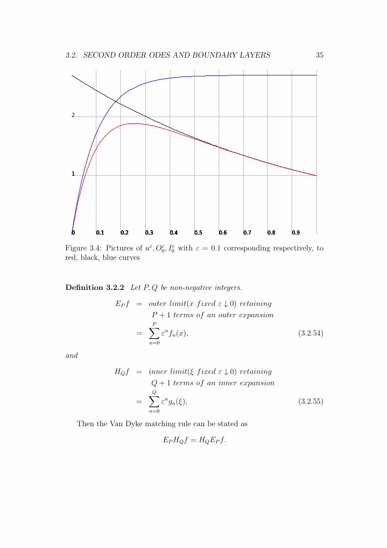
3.2. SECOND ORDER ODES AND BOUNDARY LAYERS 35
Figure 3.4: Pictures of uε, Oε0, I
ε0 with ε = 0.1 corresponding respectively, to
red, black, blue curves
Definition 3.2.2 Let P,Q be non-negative integers.
EPf = outer limit(x fixed ε ↓ 0) retaining
P + 1 terms of an outer expansion
=P∑
n=0
εnfn(x), (3.2.54)
and
HQf = inner limit(ξ fixed ε ↓ 0) retaining
Q+ 1 terms of an inner expansion
=
Q∑n=0
εngn(ξ), (3.2.55)
Then the Van Dyke matching rule can be stated as
EPHQf = HQEPf.
36 CHAPTER 3. ORDINARY DIFFERENTIAL EQUATIONS
Example 3.2.1 Let P = Q = 0. For our problem in this section, we definef = uε, and H0g := A0(e
−ξ − 1), E0f := e1−x. Then
E0H0g = E0A0(e−ξ − 1)
= E0A0(e−x/ε − 1)
= −A0. (3.2.56)
and
H0E0f = H0e1−x= H0e1−εξ= e. (3.2.57)
By the Van Dyke rule, (3.2.56) must coincide with (3.2.57), and we obtainagain
A0 = −e,
which is (3.2.42).We can also derive the matching conditions of higher order, see the following
example:Example 3.2.2 Let P = Q = 1. For our problem in this section, we definef = uε, and H1g := A0(e
−ξ − 1) + ε(A1(e−ξ − 1)− eξ), E1f := e1−x. Then
E1H1g = E1A0(e−ξ − 1) + ε(A1(e
−ξ − 1)− eξ)= E1A0(e
−x/ε − 1) + ε(A1(e−x/ε − 1)− ex/ε)
= A0 − ex+ εA1, (3.2.58)
and
H1E1f = H1e1−x= H1e1−εξ= H1e(1− εξ +O(ε2))= e(1− εξ). (3.2.59)
By the Van Dyke rule, (3.2.58) must coincide with (3.2.59), and hence
A0 = −e, A1 = 0.
which are (3.2.42) and (3.2.46).
However, for some problems, the Van Dyke rule for matching does notwork. Some examples are given in the next subsection.
3.2. SECOND ORDER ODES AND BOUNDARY LAYERS 37
3.2.4 Examples that the matching condition does notexist
Consider the following terrible problem: The function like
ln(1 + ln r/ ln1
ε).
For this function Van Dyke’s rule fails for all values of P and Q. The inter-mediate variable method of matching also struggles, because the leading orderpart of an infinite number of terms must be calculated before the matching canbe made successfully. It is unusual to find such a difficult problem in practice.See the book by Hinch [22].
3.2.5 Matched asymptotic expansions
In this subsection we shall make use of the inner and outer expansions toconstruct approximations. Also we do it in two ways.
i) The first method: Adding inner and outer expansions, then subtractingthe common part, we obtain
U ε0 (x) = e1−x + e(1− e−ξ)− e = e(e−x − e−
xε )
U ε1 (x) = e(e−x − e−
xε )− ex− (−eεξ) = e(e−x − e−
xε )
U ε2 (x) = e(e−x − e−
xε ) +
1
2ex2 − 1
2e(εξ)2 = e(e−x − e−
xε ). (3.2.60)
From which one asserts that
U ε0 (x) = U ε
1 (x) = U ε2 (x).
Therefore, more terms we take for an approximation, but the accuracyof this approximation is not more greater! This is a phenomenon which isdifferent from what we have had for algebraic equations.
ii) The second method: Employing the cut-off function defined in previoussubsection. Then we get
U εi (x) = (1− χε(x))O
εi (x) + χε(x)I
εi (x
ε). (3.2.61)
Here, i = 0, 1, 2.
38 CHAPTER 3. ORDINARY DIFFERENTIAL EQUATIONS
3.3 Examples
The following examples will help us to clarify some ideas about the method ofasymptotic expansions.
Example 3.3.1 The problems we discussed have only one boundary layer.However, in some singular perturbation problems, more than one boundarylayer can occur. This is exemplified by
εd2u
dx2− u = A, in D. (3.3.1)
u(0) = α, (3.3.2)
u(1) = β. (3.3.3)
Here A = 0, β = 0.
Example 3.3.2 A problem can be singular although ε does not multiply thehighest order derivative of the equation. A simple example is the following:
∂2u
∂x2− ε
∂u
∂y= 0, in D = (x, y) | 0 < x < 1, 0 < y < y0. (3.3.4)
u(x, 0; ε) = f(x), for 0 ≤ x ≤ 1, (3.3.5)
u(0, y; ε) = g1(y), for 0 ≤ y ≤ y0, (3.3.6)
u(1, y; ε) = g2(y), for 0 ≤ y ≤ y0, (3.3.7)
where we have taken y0 > 0, and chosen u0 satisfying ∂2u0
∂x2 = 0 as follows
u0(x, y; ε) = g1(y) + (g2(y)− g1(y))x.
However, in general, u0(x, 0; ε) = f(x), so that u0 is not an approximation ofu in D.
This can be easily understood by noting that (3.3.4) is parabolic while itbecomes elliptic if ε = 0.
Example 3.3.3 In certain perturbation problems, there exists a uniquelydefined function u0 in D satisfying the limit equation L0u0 = f0 and all theboundary conditions imposed on u, and yet u0 is not an approximation of u:
(x+ ε)2du
dx+ ε = 0, for 0 < x < A, (3.3.8)
u(0; ε) = 1. (3.3.9)
We have the exact solution to problem (3.3.8) – (3.3.9):
u = u(x; ε) =ε
x+ ε,
3.3. EXAMPLES 39
and
L0 = x2d
dx.
The function u0 = 1 satisfies L0u0 = 0 and also the boundary conditions. But
limε→0
u(x; ε) =
0 if x = 0,1 if x = 0,
(3.3.10)
and
maxD
|u− u0| =A
A+ ε→ 0
as ε→ 0.
Example 3.3.4 Some operators Lε cannot be decomposed into an “unper-turbed ε-independent part” and “a perturbation”.
du
dx− ε exp(−(u− 1)/ε) = 0, for D = 0 < x < A, (3.3.11)
u(0; ε) = 1− α. (3.3.12)
Here α > 0. Note that
limε→0
maxD
(ε exp(−(g − 1)/ε))
= 0
if and only if g > 1 for x ∈ D. Thus we do not have the decomposition withL0 =
ddx. Moreover, from the exact
u(x; ε) = 1 + ε log(x+ exp(−α/ε)),
we assert easily that none of the “usually” successful methods produces anapproximation of u in D.

40 CHAPTER 3. ORDINARY DIFFERENTIAL EQUATIONS
Chapter 4
Partial differential equations
4.1 Regular problem
Let D be an open bounded domain in Rn with smooth boundary ∂D, heren ∈ N. Consider
∆u+ εu = f0 + εf1, in D, (4.1.1)
u|∂D = 0. (4.1.2)
The associated limit problem is
∆u = f0, in D, (4.1.3)
u|∂D = 0. (4.1.4)
We shall prove this is a regular problem under suitable assumptions on thedata f0, f1. Let u
ε, u0 be solutions to problems (4.1.1) – (4.1.2) and (4.1.3) –(4.1.4), respectively. Define vε = uε − u0, then vε satisfies
∆vε = −εuε + εf1, (4.1.5)
vε|∂D = 0. (4.1.6)
Assume that f0, f1 ∈ Cα(D) for some α ∈ (0, 1). Applying the Schaudertheory for elliptic equations, from equation (4.1.5) we assert that
∥uε∥C2,α(D) ≤ C(?∥uε∥L∞(D) + ∥f0∥Cα(D) + ∥f1∥Cα(D)), (4.1.7)
hence, from (4.1.1) we obtain
∥vε∥C2,α(D) ≤ Cε(∥uε∥Cα(D) + ∥f1∥Cα(D))
≤ Cε(∥f0∥Cα(D) + ∥f1∥Cα(D)). (4.1.8)
41
42 CHAPTER 4. PARTIAL DIFFERENTIAL EQUATIONS
Then one can conclude easily that
∥vε∥C0(D) → 0, i.e. ∥uε − u0∥C0(D) → 0 (4.1.9)
as ε→ 0. Therefore, problem (4.1.1) – (4.1.2) is regular.However, as we pointed out in Example 2 in Section 3.3, there are some
problems which are singular though the small parameter does not multiply thehighest order derivative. We shall give another example in next section.
4.2 Conservation laws and vanishing viscosity
method
In this section we will study the inviscid limit of scalar conservation laws withviscosity.
ut + (F (u))x = νuxx, (4.2.1)
u|t=0 = u0. (4.2.2)
The associated inviscid problem is
ut + (F (u))x = 0, (4.2.3)
u|t=0 = u0. (4.2.4)
It is a basic question that does the solution of (4.2.1) – (4.2.2) converge tothat of (4.2.3) – (4.2.4)? This is the main problem for the method of vanishingviscosity.
In this section we are going to prove that the answer to this question ispositive under some suitable assumptions. We shall make use of the method ofmatched asymptotic expansions and L2-energy method. First of all, we makethe following assumptions.
Assumptions. A1)
The function F is smooth. (4.2.5)
A2) Let n ∈ N. g0, h0 ∈ L1(R) ∩ L∞(R), g0x ∈ L1(R) and pTn ∈ L1(R) ∩Liploc(R) ∩ L∞(R). g0x, h0 have only a shock at φI , respectively. There existsmooth functions gε, hε, pTn,ε ∈ C∞
0 (R), such that
gε, hε, pTn,ε → g0, h0, pTn (4.2.6)
in L2(R) as ε → 0, respectively. Moreover, we assume that pTn is boundedsequence in BV loc(R) such that as n→ ∞,
pTn → pT in L1loc(R). (4.2.7)
4.2. CONSERVATION LAWS AND VANISHING VISCOSITY METHOD43
A3) Assume further that Oleinik’s one-sided Lipschitz condition (OSLC)is satisfied, i.e.
(f(u(x, t))− f(u(y, t))) (x− y) ≤ α(t)(x− y)2 (4.2.8)
for almost every x, y ∈ R and t ∈ (0, T ), where α ∈ L1(0, T ).
4.2.1 Construction of approximate solutions
4.2.1.1 Outer and inner expansions
First of all, we expand the nonlinearity F (u) as
F (η) = F (η0) + νf(η0)η1 + ν2(f(η0)η2 +
1
2f(η0)(η1)
2
)+ · · · , (4.2.9)
f(η) = f(η0) + νf ′(η0)η1 + ν2(f ′(η0)η2 +
1
2f ′′(η0)(η1)
2
)+ · · · .(4.2.10)
Step 1. To construct outer expansions, we begin with the definition of anansatz
uν(x, t) = u0(x, t) + νu1(x, t) + ν2u2(x, t) + · · · . (4.2.11)
Inserting this into equation (4.2.2) and balancing both sides of the resultingequation yield
ν0 : (u0)t + (F (u0))x = 0, (4.2.12)
ν1 : (u1)t + (f(u0)u1)x = R, (4.2.13)
ν2 : (u2)t + (f(u0)u2)x = R1, (4.2.14)
where R and R1 are functions defined by
R := u0,xx − σ(u0,xψ
′ + ((u0,x)t + (f(u0)u0,x)x)ψ)
and
R1 :=
(1
2u0,xσψ + u1
)xx
−(1
2u0,xx(σψ)
2 + u1,xσψ
)t
−(f(u0)
(1
2u0,xx(σψ)
2 + u1,xσψ
)+
1
2f ′(u0)(u0,xσψ + u1)
2
)x
(4.2.15)
from which we see that R, R1 depend on constant σ and functions ψ, u0 andu1.
44 CHAPTER 4. PARTIAL DIFFERENTIAL EQUATIONS
Step 2. Next we construct inner expansions. Introduce a new variable
ξ =x− φ(t)
ν.
uε(x, t) = U0(ξ, t) + νU1(ξ, t) + ν2U2(ξ, t) + · · · . (4.2.16)
Substituting this ansatz into equation, equating the coefficients of νi (withi = −1, 0, 1) on both sides of resultant, we obtain
ν−1 : U ′′0 + φU ′
0 − (F (U0))′ = 0, (4.2.17)
ν0 : U ′′1 + φU ′
1 − (f(U0)U1)′ = −σψU ′
0 + U0t, (4.2.18)
ν1 : U ′′2 + φU ′
2 − (f(U0)U2)′ = −σψu′1
(f ′(u0)
2U21
)′
+ U1t. (4.2.19)
Some orthogonality condition should be satisfied.
4.2.1.2 Matching conditions and approximations
Step 3. This step is to find the matching conditions and then to constructapproximations. Suppose that there is a uniform asymptotic expansion, thenthere holds for any fixed t and large ξ
U0(ξ, t) + νU1(ξ, t) + ν2U2(ξ, t) = u0(x, t) + νu1(x, t) + ν2u2(x, t) +O(ν3).
Using the technique in [14] again, we rewrite the right hand side of the aboveequality in terms of ξ, t, and make use of Taylor expansions to obtain
U0(ξ, t) + νU1(ξ, t) + ν2U2(ξ, t)
= u0(νξ, t) + νu1(νξ, t) + ν2u2(νξ, t) +O(ν3)
= u0(0, t) + u′0(0, t)εξ +1
2u′′0(0, t)(νξ)
2
+ν(u1(0, t) + u′1(0, t)νξ) + ν2u2(0, t) +O(ν3)
= u0(0, t) + ν(u′0(0, t)ξ + u1(0, t))
+ν2(1
2u′′0(0, t)ξ
2 + u′1(0, t)ξ) + u2(0, t)
)+O(ν3). (4.2.20)
Hence it follows that
U0(ξ, t) = u0(0, t), (4.2.21)
U1(ξ, t) = u1(0, t) + u′0(0, t)ξ, (4.2.22)
U2(ξ, t) = u2(0, t) +1
2u′′0(0, t)ξ
2 + u′1(0, t)ξ). (4.2.23)
4.3. CONVERGENCE OF THE APPROXIMATE SOLUTIONS 45
Thus we establish a uniform approximation up to order O(ν2) by employinga cut-off function. Define
Oν2(x, t) = u0(x, t) + νu1(x, t) + ν2u2(x, t), (4.2.24)
Iν2 (x, t) = U0(x, t) + νU1(x, t) + ν2U2(x, t). (4.2.25)
Then a uniform asymptotic expansion can be constructed
U ν2 (x, t) = χν(x, t)O
ν2(x, t) + (1− χν(x, t))I
ν2 (x− φ(t)
ν, t). (4.2.26)
4.2.2 Convergence
This subsection is devoted to the investigation of convergence of the approxi-mation obtained in Subsection 4.1. Firstly, we prove that the approximationsatisfies equation (4.2.1) asymptotically. That is
(U ν2 )t + (f(U ν
2 ))x − ν(U ν2 )xx = O(να). (4.2.27)
Secondly, the approximation uν converges to the solution u0 to the corres-ponding limit problem (4.2.3) – (4.2.4), as ν → 0. The main result is
Theorem 4.2.1 Suppose that the condition (5.3.75) and assumptions (5.3.7)– (5.3.10) are satisfied and that ε = σν with σ being a positive constant.
Then the approximate solutions U ν2 , V
ν2 , P
ν2 satisfy respectively, equations
(5.3.1), (5.3.3) and (5.3.5), in the following sense
(U ν2 )t − ν(U ν
2 )xx + (F (U ν2 ))x = O(να) (4.2.28)
where α = 3γ − 1 and γ ∈ (13, 1).
4.3 Convergence of the approximate solutions
This section is devoted to the proof of following Theorem 4.1, which consistsof two parts, one is to prove Theorem 3.1 which asserts that the equations aresatisfied asymptotically, and another is to investigate the convergence rate.
Theorem 4.3.1 Suppose that the assumptions in Theorem 3.1 are met. Letu, p be, respectively, the unique entropy solution with only one shock, the re-versible solution to problems (5.1.1) – (5.1.2) and (5.1.8) – (5.1.9), and let vbe the unique solutions to problem (5.3.62) – (5.3.65), such that∫ T
0
∫x =φ(t), t∈[0,T ]
6∑i=1
(|∂ixu(x, t)|2 + |∂ixv(x, t)|2 + |∂ixp(x, t)|2
)dxdt ≤ C.(4.3.1)
46 CHAPTER 4. PARTIAL DIFFERENTIAL EQUATIONS
Then the solutions (uν , vν) of problems (5.3.1) – (5.3.2) and (5.3.3) – (5.3.4)converge, respectively, to (u, v) in L∞(0, T ;L2(R))×L∞(0, T ;L2(R)), and thefollowing estimates hold
sup0≤t≤T
∥uν(t)− u(t)∥+ sup0≤t≤T
∥vν(t)− v(t)∥ ≤ Cηνη. (4.3.2)
Here η is a constant defined by
η = min
3
2γ,
1 + γ
2
, where γ is the same as in Theorem 3.1, (4.3.3)
Remark 4.1. Combination of (5.4.4) and a stability theorem of the reversiblesolutions (see Theorem 4.1.10 in Ref. [6])) yields that
sup0≤t≤T
∥pν,n − p∥L∞(Ωh∩[−R,R]) → 0, (4.3.4)
as ν → 0, then n → ∞, where R is any positive constant. This ensures us toselect alternating descent directions.
4.3.1 The equations are satisfied asymptotically
In this sub-section, we are going to prove that the approximate solutionsU ν2 , V
ν2 , P
ν2 satisfy asymptotically, the corresponding equations (5.3.1), (5.3.3)
and (5.3.5) respectively. For simplicity, in this sub-section we omit the super-script ν and write the approximate solutions as U2, V2, P2.
Proof of Theorem 3.1. We divide the proof into three parts.
Part 1. We first investigate the convergence of U2. Straightforward computa-tions yield
(U2)t =dtνγχ′ν
(U2 − U2
)+ χν · (U2)t + (1− χν)(U2)t, (4.3.5)
(U2)x =1
νγχ′ν
(U2 − U2
)+ χν · (U2)x + (1− χν)(U2)x, (4.3.6)
(U2)xx =1
ν2γχ′′ν
(U2 − U2
)+
2
νγχ′ν
(U2 − U2
)x
+χν · (U2)xx + (1− χν)(U2)xx. (4.3.7)
Hereafter, to write the derivatives of U2 in the form, like the first term in theright hand side of (5.4.7), we changed the arguments t, x of U2, V2, P2 to t, d,where d = d(x, t) is defined by
d(x, t) = x− φ(t).
4.3. CONVERGENCE OF THE APPROXIMATE SOLUTIONS 47
However, risking abuse of notations we still denote U2(d, t), V2(d, t), P2(d, t) byU2, V2, P2 for the sake of simplicity. After such a transformation of arguments,the terms are easier to deal with, as we shall see later on.
Therefore, we find that U2 satisfies
(U2)t − ν (U2)xx + (F (U2))x = I1 + I2 + I3, (4.3.8)
where Ik (k = 1, 2, 3) are the collections of like-terms according to whether ornot their supports are contained in a same sub-domain of R, more precisely,they are defined by
I1 = χν
((U2)t − ν(U2)xx + f(U2) · (U2)x
), (4.3.9)
I2 = (1− χν)((U2)t − ν(U2)xx + f(U2)(U2)x
), (4.3.10)
I3 = (U2 − U2)
(dtχ
′ν
νγ− χ′′
ν
ν2γ−1+χ′νf(U2)
νγ
)− 2χ′
ν
νγ−1
(U2 − U2
)x.(4.3.11)
It is easy to see that the support of I1, I2 is, respectively, a subset of[0, 2νγ] and a subset of [νγ,∞), while the support of I3 is a subset of [νγ, 2νγ]∪[−2νγ,−νγ].
Now we turn to estimate I1, I2, I3. Firstly we handle I3. In this case onecan apply the matching conditions (5.3.72) – (5.3.74) and use Taylor expan-sions to obtain
∂lx(U2 − U2)(x, t) = O(1)ν(3−l)γ (4.3.12)
on the domain (x, t) | νγ ≤ |x − φ(t)| ≤ 2 νγ, 0 ≤ t ≤ T and l = 0, 1, 2, 3.From these estimates (5.4.14), which can also be found, e.g. in Goodman andXin [21], the following assertion follows easily that
I3 = O(1)ν2γ as ν → 0. (4.3.13)
Moreover, we have∫R|I3(x, t)|2dx =
∫νγ≤|x−φ(t)|≤2 νγ
|I3(x, t)|2dx ≤ Cν5γ. (4.3.14)
To deal with I1, I2 we rearrange the terms of I1, I2 as follows
I1 = χν
((U2)t − ν(U2)xx + (F (U2))x
)+ χν ·
(f(U2)− f(U2)
)(U2)x,
= I1a + I1b, (4.3.15)
I2 = (1− χν)((U2)t − ν(U2)xx + (F (U2))x
)+ (1− χν)
(f(U2)− f(U2)
)(U2)x,
= I2a + I2b. (4.3.16)
48 CHAPTER 4. PARTIAL DIFFERENTIAL EQUATIONS
Moreover, I1b can be rewritten as
I1b = χν
∫ 1
0
f ′(sU2 + (1− s)U2)ds · (U2 − U2)(U2)x. (4.3.17)
Note that supp I1b ⊂ (x, t) ∈ QT | |x − φ(t)| ≤ 2 νγ and U2(x, t) = U2(x, t)if (x, t) ∈ QT | |x − φ(t)| ≤ νγ. Therefore, from (5.4.14) and (5.4.19) weobtain
|I1b| =C
ν|(U2 − U2)(U2)
′| = O(ν3γ−1), (4.3.18)
where we choose γ > 13so that 3γ − 1 > 0. Recalling the construction of U2,
from equations (5.3.69) – (5.3.71), we can rewrite I1a as
I1a = χν
((U2)t − ν(U2)xx + (F (u0) + νf(u0)u1 + ν2(f(u0)u2 +
1
2f ′(u0)u
21) +Ru)x
)= χν(Ru)x, (4.3.19)
where the remainder Ru is defined by
Ru = F (U2)−(F (u0) + νf(u0)u1 + ν2(f(u0)u2 +
1
2f ′(u0)u
21)
)= O(ν3).
Thus
|I1a| ≤ |(Ru)x| =1
ν|(Ru)
′| = O(ν2). (4.3.20)
In a similar manner, we now handle I2, and rewrite I2b as
I2b = (1− χν)
∫ 1
0
f ′(sU2 + (1− s)U2)ds · (U2 − U2)(U2)x. (4.3.21)
It is easy to see that supp I2b ⊂ |d| ≥ νγ and U2 = U2 if |d| ≥ 2νγ. From thefact that U2 − U2 = χν(U2 − U2) and (5.4.14) it follows that
|I2b| ≤ C χν |(U2 − U2)(U2)x| = O(ν3γ). (4.3.22)
As for I2a, invoking equations (5.3.29) and (5.3.30) we assert that there holds
I2a = (1− χν)((U2)t − ν(U2)xx + (F (u0) + νf(u0)u1 +Ru)x
)= (1− χν)(Ru)x +O(ν2). (4.3.23)
and the remainder Ru is given by
Ru = F (U2)− (F (u0) + νf(u0)u1) = O(ν2),
4.3. CONVERGENCE OF THE APPROXIMATE SOLUTIONS 49
hence
I2a = O(ν2). (4.3.24)
On the other hand, we have∫R|I1(x, t)|2dx =
∫|x−φ(t)|≤2 νγ
|I1(x, t)|2dx
≤∫|x−φ(t)|≤νγ
|I1a(x, t)|2dx+∫νγ≤|x−φ(t)|≤2 νγ
|I1b(x, t)|2dx
≤ C(ν2∗2+1 + ν6γ−2+γ) ≤ C νγ. (4.3.25)
Here we used the simple inequalities: 6γ − 2 + γ < 5 and 6γ − 2 > 0 since weassume γ ∈ (1
3, 1).
Similarly, one can obtain∫R|I2(x, t)|2dx =
∫|x−φ(t)|≥νγ
|I2(x, t)|2dx ≤ C(ν2∗2+1 + ν6γ+γ) ≤ C νγ.(4.3.26)
In conclusion, from (5.4.10), (5.4.15), (5.4.20), (5.4.22), (5.4.24) and (5.4.26)we are in a position to assert that U ν
2 satisfies the equation in the followingsense
(U ν2 )t − ν(U ν
2 )xx + (F (U ν2 ))x = O(να),
as ν → 0. Here α = 3γ − 1 and we used the fact that 3γ − 1 < 2γ < 2by assumption γ < 1. Furthermore, from construction we see easily that theinitial data is satisfied asymptotically too.
Part 2. We now turn to investigate the convergence of V2. Similar computa-tions show that V2 can be written in terms of V2, V2 as
(V2)t =dtνγχ′ν
(V2 − V2
)+ χν · (V2)t + (1− χν)(V2)t, (4.3.27)
(V2)x =1
νγχ′ν
(V2 − V2
)+ χν · (V2)x + (1− χν)(V2)x, (4.3.28)
(V2)xx =1
ν2γχ′′ν
(V2 − V2
)+
2
νγχ′ν
(V2 − V2
)x
+χν · (V2)xx + (1− χν)(V2)xx, (4.3.29)
and V2 satisfies the following equation
(V2)t − ν (V2)xx + (f(U2)V2)x = J1 + J2 + J3, (4.3.30)
50 CHAPTER 4. PARTIAL DIFFERENTIAL EQUATIONS
where Jk (k = 1, 2, 3) are given, according to their supports, by
J1 = χν
((V2)t − ν(V2)xx +
(f(U2)V2
)x
), (4.3.31)
J2 = (1− χν)((V2)t − ν(V2)xx +
(f(U2)V2
)x
), (4.3.32)
J3 =
(dtχ
′ν
νγ− χ′′
ν
ν2γ−1+f(U2)χ
′ν
νγ
)(V2 − V2)−
2χ′ν
νγ−1(V2 − V2)x.(4.3.33)
Since for V2, we also have the same estimate (5.4.14) which is valid for U2,namely we have
∂lx(V2 − V2) = O(1)ν(3−l)γ (4.3.34)
on the domain (x, t) | νγ ≤ |x − φ(t)| ≤ 2 νγ, 0 ≤ t ≤ T and l = 0, 1, 2, 3.Thus it follows from (5.4.36) and the uniform boundedness of U2 that
J3 = O(1)ν2γ, as ν → 0. (4.3.35)
The investigation of convergence for J1, J2 is more technically complicatedthan I1, I2. Rewrite J1, J2 as
J1 = χν
((V2)t − ν(V2)xx + (f(U2)V2)x
)+ χν ·
((f(U2)− f(U2)) V2
)x
= J1a + J1b, (4.3.36)
and
J2 = (1− χν)((V2)t − ν(V2)xx + (f(U2)V2)x
)+ (1− χν)
((f(U2)− f(U2)V2
)x
= J2a + J2b. (4.3.37)
We now deal with J1b which can be changed to
J1b = χν
(∫ 1
0
f ′(sU2 + (1− s)U2)ds(U2 − U2) V2
)x
= χν
(∫ 1
0
f ′(sU2) + (1− s)U2)ds V2
)x
(U2 − U2)
+χν
∫ 1
0
f ′(sU2) + (1− s)U2)ds V2
(U2 − U2
)x
= O(ν3γ−1) +O(ν2γ) = O(ν3γ−1), (4.3.38)
here we used that 3γ − 1 < 2γ since γ < 1.
4.3. CONVERGENCE OF THE APPROXIMATE SOLUTIONS 51
Rewriting J1a as
J1a = χν
((V2)t − ν(V2)xx +
((f(u0) + f ′(u0)(νu1 + ν2u2) +
1
2f ′′(u0)(νu1)
2)V2
)x
)+χν(RvV2)x
= χν
(O(ν2) + (RvV2)x
). (4.3.39)
Here, equations (5.3.76) - (5.3.78) were used. And the remainder Rv is
Rv = f(U2)− (f(u0) + f ′(u0)(νu1 + ν2u2) +1
2f ′′(u0)(νu1)
2) = O(ν3)
Therefore, from (5.4.41) one has
J1a = χν
(O(ν2) + (RvV2)x
)= O(ν2). (4.3.40)
The terms J2a, J2b can be estimated in a similar way and we obtain
J2b = O(ν3γ) +O(ν2γ) = O(ν2γ), (4.3.41)
and
J2a = (1− χν)((V2)t − ν(V2)xx + ((f(u0) + νf ′(u0)u1 +Rv)V2)x
)= (1− χν)
(O(ν2) + (RvV2)x
),
where Rv is given by Rv = f(U2)− (f(u0) + νf ′(u0)u1) = O(ν2). It is easy tosee that
J2a = O(ν2). (4.3.42)
On the other hand, we have the following estimates of integral type∫R|J1(x, t)|2dx =
∫|x−φ(t)|≤2 νγ
|J1(x, t)|2dx
≤∫|x−φ(t)|≤νγ
|J1a(x, t)|2dx+∫νγ≤|x−φ(t)|≤2 νγ
|J1b(x, t)|2dx
≤ C(ν2∗2+1 + ν6γ−2+γ) ≤ C νγ. (4.3.43)
and∫R|J2(x, t)|2dx =
∫|x−φ(t)|≥νγ
|J2(x, t)|2dx ≤ C(ν2∗2+1 + ν4γ+γ) ≤ C νγ.(4.3.44)
52 CHAPTER 4. PARTIAL DIFFERENTIAL EQUATIONS
Therefore, it follows from (5.4.32), (5.4.37), (5.4.40), (5.4.42), (5.4.43) and(5.4.44) that V ν
2 satisfies the equation in the following sense
(V ν2 )t − ν(V ν
2 )xx + (f(U ν2 )V
ν2 )x = O(ν3γ−1),
as ν → 0. By construction, the initial data is satisfied asymptotically as well.
Part 3. Finally we turn to investigate the convergence of P2. Computationsshow that the derivatives of P2 can be written in terms of P2, P2 as
(P2)t =dtνγχ′ν
(P2 − P2
)+ χν · (P2)t + (1− χν)(P2)t, (4.3.45)
(P2)x =1
νγχ′ν
(P2 − P2
)+ χν · (P2)x + (1− χν)(P2)x, (4.3.46)
(P2)xx =1
ν2γχ′′ν
(P2 − P2
)+
2
νγχ′ν
(P2 − P2
)x
+χν · (P2)xx + (1− χν)(P2)xx, (4.3.47)
and P2 satisfies the following equation
−(P2)t − ν (P2)xx − f(U2)(P2)x = K1 +K2 +K3, (4.3.48)
where Ki (i = 1, 2, 3) are given, according to their supports, by
K1 = −χν
((P2)t + ν(P2)xx + f(U2)(P2)x
), (4.3.49)
K2 = −(1− χν)((P2)t + ν(P2)xx + f(U2) (P2)x
), (4.3.50)
K3 = −
(dtχ
′ν
νγ+
χ′′ν
ν2γ−1+f(U2)χ
′ν
νγ
)(P2 − P2)−
2χ′ν
νγ−1(P2 − P2)x.(4.3.51)
By similar arguments as done for U ν2 , we can prove that
−(P ν2 )t − ν(P ν
2 )xx − f(U ν2 )(P
ν2 )x = O(ν3γ−1),
as ν → 0.
4.3.2 Proof of the convergence
This sub-section is devoted to the proof of Theorem 4.1. Since this sub-sectionis concerned with the proof of convergence as ν → 0, we denote U ν
2 , Vν2 , P
ν2
by U ν , V ν , P ν , respectively, for the sake of simplicity. We begin with thefollowing lemma.
4.3. CONVERGENCE OF THE APPROXIMATE SOLUTIONS 53
Lemma 4.3.2 For η defined in (5.4.5),
sup0≤t≤T
∥uν(·, t)− u(·, t)∥+ sup0≤t≤T
∥vν(·, t)− v(·, t)∥ ≤ Cνη, (4.3.52)
sup0≤t≤T
∥pν,n(·, t)− p(·, t)∥L1loc(R) → 0, (4.3.53)
as ν → 0, then n → ∞. Here pν,n denotes the solution to smoothed adjointproblem (5.3.5) – (5.3.6).
Proof. Firstly, by construction of the approximate solutions, we conclude thati) for (x, t) ∈ |x− φ(t)| ≥ 2νγ, 0 ≤ t ≤ T,
Uν2 (x, t) = u(x, t) +O(1)ν,
where O(1) denotes a function which is square-integrable over outer region bythe argument in sub-section 4.1.ii) for (x, t) ∈ |x− φ(t)| ≤ νγ,
U ν2 (x, t) = u0(x, t) +O(1)νγ,
iii) and for (x, t) ∈ νγ ≤ |x− φ(t)| ≤ 2νγ,
U ν2 (x, t) = U ν
2 (x, t) + χν(x, t)(Uν2 (x, t)− Uν
2 (x, t)) ∼ U ν2 (x, t) +O(1)ν3γ.
Here we have used again the estimate U ν2 (x, t) − U ν
2 (x, t) = O(1)ν3γ. We canalso establish similar estimates for V ν
2 , Pν2 . Therefore, one can obtain
sup0≤t≤T
∥u(·, t)− U ν(·, t)∥2 + sup0≤t≤T
∥v(·, t)− V ν(·, t)∥2 ≤ Cνmin3γ,2,(4.3.54)
sup0≤t≤T
∥pn(·, t)− P ν(·, t)∥2 ≤ Cνmin3γ,2,(4.3.55)
where pn is the reversible solution to the inviscid adjoint equation −∂tp −f(u)∂xp = 0 with final data p(x, T ) = pTn (x).
By Theorem 4.1.10 which is concerned with the stability (with respect tocoefficient and final data) of reversible solutions in [6] (see also Theorem 5.1in the appendix of this chapter), and the assumptions of final data pn and theone-sided Lipschitz condition we conclude that the reversible solution pn of thebackward problem with initial data pn satisfies
pn → p in C([0, T ]× [−R,R])
for any R > 0, here p is the reversible solution to −pt − f(u)∂xp = 0, inR× (0, T ) with finial data p(x, T ) = pT (x) for x ∈ R. Therefore, we have
sup0≤t≤T
∥pn − p∥L1loc(R) → 0, (4.3.56)
54 CHAPTER 4. PARTIAL DIFFERENTIAL EQUATIONS
as n→ ∞.Secondly, we need to estimate sup0≤t≤T ∥uν(·, t)− U ν(·, t)∥2, etc. Suppose
that we have obtained
sup0≤t≤T
∥uν(·, t)− U ν(·, t)∥2 ≤ Cνη1 (4.3.57)
where η1 = γ + 1. Then we arrive at (5.4.54) by using the triangle inequality,the estimate (5.4.56) and the fact that min
32γ, 1+γ
2, 1= min
32γ, 1+γ
2
(since
13< γ < 1)). So we conclude for v, p.
Part 1. Now we prove (5.4.59). To this end, we define
w(x, t) = uν(x, t)− U ν(x, t),
Then w(x, t) satisfies
wt − νwxx + f(uν)wx = F , (4.3.58)
w(x, 0) = w0(x). (4.3.59)
Here
F := −3∑
i=1
Ii −Q(x, t)− f ′(Uν)wU νx (4.3.60)
Q :=(f(uν)− f(U ν)− f ′(U ν)w
)U νx . (4.3.61)
Rescaling as follows
w(x, t) = νw(y, τ), where y =x− φ(t)
ν, and τ =
t
ν,
one has
wt(x, t) = wτ (y, τ)−φ′(ντ)wy, wx(x, t) = wy(y, τ), wxx(x, t) =1
νwyy(y, τ),
and problem (5.4.60) – (5.4.61) turns out to be
wτ − wyy + (f(uν)− φ′(ντ))wy = F(νy + φ, ντ), (4.3.62)
w(x, 0) = w0(x). (4.3.63)
Here the initial data w0 can be chosen very small such that
∥w0∥2H1(R) ≤ Cν ≤ Cνγ,
provided that ν is suitably small.The existence of solution w ∈ C([0, T/ν];H1(R)) to problem (5.4.64) –
(5.4.65) follows from the method of continuation of local solution, which is ba-sed on local existence of solution and a priori estimates stated in the followingproposition
4.3. CONVERGENCE OF THE APPROXIMATE SOLUTIONS 55
Proposition 4.3.3 (A priori estimates) Suppose that problem (5.4.64) – (5.4.65)has a solution w ∈ C([0, τ0];H
1(R)) for some τ0 ∈ (0, T/ν]. There exists posi-tive constants µ1, ν1 and C, which are independent of ν, τ0, such that if
ν ∈ (0, ν1], sup0≤τ≤τ0
∥w(τ, ·)∥H1(R) + µ0 ≤ µ1, (4.3.64)
then
sup0≤τ≤τ0
∥w(τ, ·)∥2H1(R) +
∫ τ0
0
∥w(τ, ·)∥2H2(R)dτ ≤ Cνγ.
Proof. Step 1. By the maximum principle and construction of approximatesolution U ν , we have
∥uν∥L∞(Qτ0 )≤ C, ∥U ν∥L∞(Qτ0 )
≤ C. (4.3.65)
Whence, from the smallness assumption (5.4.66) and definition of Q it followsthat
|Q(x, t)| ≤ C|w2U νx |. (4.3.66)
Step 2. Multiplying eq. (5.4.64) by w and integrating the resulting equa-tion with respect to y over R we obtain
1
2
d
dτ∥w∥2 + ∥wy∥2 +
∫R(f(uν)− φ′(ντ))wywdy =
∫RF(νy + φ, ντ)wdy.(4.3.67)
We first deal with the term∫Rf ′(U ν)wU ν
xwdy =
∫Rf ′(U ν)w2νU ν
xdy.
From the property of profile U we have
νU νx = U ν
y → 0, as ν → 0.
Thus ∣∣∣∣∫Rf ′(Uν)wU ν
xwdy
∣∣∣∣ ≤ C∥w∥2.
For the term of Q, it is easier to obtain that∣∣∣∣∫RQ(y, τ)U ν
xwdy
∣∣∣∣ ≤ C
∫R|w2Uν
xw|dy ≤ C∥w∥2.
56 CHAPTER 4. PARTIAL DIFFERENTIAL EQUATIONS
It remains to deal with the term∫R Iwdy where I =
∑3i=1 Ii. We invoke the
L2-norm estimates for I, i.e. (5.4.27) and (5.4.28), which have been obtainedin Subsection 3.1, and get∣∣∣∣∫ τ
0
∫RIwdτdy
∣∣∣∣ ≤ C
(∫ τ
0
∫R|I|2dτdy +
∫ τ
0
∫R|w|2dτdy
)≤ Cνγ + C
∫ τ
0
∫R|w|2dτdy. (4.3.68)
Finally, by the Young inequality one gets∣∣∣∣∫R(f(uν)− φ′(ντ))wywdy
∣∣∣∣ ≤ 1
2∥wy∥2 + C∥w∥2.
Therefore, the above arguments and integrating (5.4.69) with respect to τyield
1
2∥w(τ)∥2 + 1
2
∫ τ
0
∥wy(s)∥2ds ≤ C
∫ τ
0
∥w(s)∥2ds+ Cνγ, (4.3.69)
from which and the Gronwall inequality in the integral form we then arrive at
∥w(τ)∥2 ≤ Cνγ.
So we also obtain
∥uν(·, t)− U ν(·, t)∥2 = ν∥w(τ)∥2 ≤ Cν1+γ.
Step 3. Next we multiply eq. (5.4.65) by −wyy and integrate the resultantwith respect to y to get
1
2
d
dτ∥wy∥2 + ∥wyy∥2 −
∫R(f(uν)− φ′(ντ))wyywydy
= −∫RF(νy + φ, ντ)wyydy, (4.3.70)
Using (5.4.67) and estimates on Ii (I = 1, 2, 3), from the Young inequality wethen arrive at
1
2∥wy(τ)∥2 +
1
2
∫ τ
0
∥wyy(s)∥2ds ≤ C
∫ τ
0
∥wy(s)∥2ds+ Cνγ, (4.3.71)
making use of Gronwall’s inequality again one has
∥wy(τ)∥2 ≤ Cνγ. (4.3.72)
Chapter 5
An application to optimalcontrol theory
5.1 Introduction
Optimal control for hyperbolic conservation laws requires a considerable analy-tical effort and computationally expansive in practice, is thus a difficult topic.Some methods have been developed in the last years to reduce the computatio-nal cost and to render this type of problems affordable. In particular, recentlythe authors of [11] have developed an alternating descent method that takesinto account the possible shock discontinuities, for the optimal control of theinviscid Burgers equation in one space dimension. Further in [12] the vanishingviscosity method is employed to study this alternating descent method for theBurgers equation, with the aid of the Hopf-Cole formula which can be foundin [24, 37], for instance. Most results in [12] are formal.
In the present chapter we will revisit this alternating descent method inthe context of one dimensional viscous scalar conservation laws with a generalnonlinearity. The vanishing viscosity method and the method of matchedasymptotic expansions will be applied to study this optimal control problemand justify rigorously the results.
To be more precise, we state the optimal problem as follows. For a givenT > 0, we study the following inviscid problem
ut + (F (u))x = 0, in R× (0, T ); (5.1.1)
u(x, 0) = uI(x), x ∈ R. (5.1.2)
Here, F : R → R, u 7→ F (u) is a smooth function, and f denotes its derivativein the following context. The case that F (u) = u2
2is studied in e.g. [11, 12].
Given a target uD ∈ L2(R) we consider the cost functional to be minimized
57
58CHAPTER 5. AN APPLICATION TO OPTIMAL CONTROL THEORY
J : L1(R) → R, defined by
J(uI) =
∫R
∣∣u(x, T )− uD(x)∣∣2 dx,
where u(x, t) is the unique entropy solution to problem (5.1.1) – (5.1.2).We also introduce the set of admissible initial data Uad ⊂ L1(R), that we
shall define later in order to guarantee the existence of the following optimi-zation problem:
Find uI,min ∈ Uad such that
J(uI,min) = minuI∈Uad
J(uI).
This is one of the model optimization problems that is often addressedin the context of optimal aerodynamic design, the so-called inverse designproblem, see e.g. [19].
The existence of minimizers has been proved in [11]. From a practicalpoint of view it is however more important to be able to develop efficientalgorithms for computing accurate approximations of discrete minimizers. Themost efficient methods to approximate minimizers are the gradient methods.
But for large complex systems, as Euler equations in higher dimensions,the existing most efficient numerical schemes (upwind, Godunov, etc.) are notdifferentiable. In this case, the gradient of the functional is not well definedand there is not a natural and systematic way to compute its variations. Dueto this difficulty, it would be natural to explore the possible use of non-smoothoptimization techniques. The following two approaches have been developed:The first one is based on automatic differentiation, and the second one isthe so-called continuous method consisting of two steps as follows: One firstlinearizes the continuous system (5.1.1) to obtain a descent direction of thecontinuous functional J , then takes a numerical approximation of this descentdirection with the discrete values provided by the numerical scheme. Howeverthis continuous method has to face another major drawback when solutionsdevelop shock discontinuities, as it is the case in the context of the hyperbolicconservation laws like (5.1.1) we are considering here.
The formal differentiation of the continuous states equation (5.1.1) yields
∂t(δu) + ∂x(f(u)δu) = 0, in R× (0, T ); (5.1.3)
But this is only justified when the state u on which the variations are beingcomputed, is smooth enough. In particular, it is not justified when the solu-tions are discontinuous since singular terms may appear on the linearizationover the shock location. Accordingly in optimal control applications we also
5.1. INTRODUCTION 59
need to take into account the sensitivity for the shock location (which hasbeen studied by many authors, see, e.g. [9, 20, 33]). Roughly speaking, themain conclusion of that analysis is that the classical linearized system for thevariation of the solutions must be complemented with some new equations forthe sensitivity of the shock position.
To overcome this difficulty, we naturally think of another way, namely, thevanishing viscosity method (as in [12], in which an optimal control problem forthe Burgers equation is studied) and add an artificial viscosity term to smooththe state equation. Equations (5.1.1) with smoothed initial datum then turnsout to be
ut + (F (u))x = νuxx, in R× (0, T ), (5.1.4)
u|t=0 = gε. (5.1.5)
Note that the Cauchy problem (5.1.4) – (5.1.5) is of parabolic type, thus fromthe standard theory of parabolic equations (see, for instance, Ladyzenskayaet al [28]) we have that the solution uν,ε of this problem is smooth. So thelinearized one of eq. (5.1.4) can be derived easily, which reads
(δu)t + (f(u)δu)x = ν(δu)xx, in R× (0, T ), (5.1.6)
δu|t=0 = hε. (5.1.7)
Here ν, ε are positive constants, δu denotes the variation of u. The initialdata gε, hε will be chosen suitably in Section 3, so that the perturbations ofinitial data and shock position are taken into account, this renders us that wecan select the alternating descent directions in the case of viscous conservationlaws.
To solve the optimal control problem, we also need the following adjointproblem, which reads
−pt − f(u)px = 0, in R× (0, T ); (5.1.8)
p(x, T ) = pT (x), x ∈ R, (5.1.9)
here, pT (x) = u(x, T ) − uD(x). And we smooth equation (5.1.8) and initialdata as follows
−pt − f(u)px = νpxx, in R× (0, T ); (5.1.10)
p(x, T ) = pTε (x), x ∈ R, (5.1.11)
Since solutions u = u(x, t; ν, ε), δu = δu(x, t; ν, ε) are smooth, shocks va-nish, instead quasi-shock regions are formed. Natural questions are arising as
60CHAPTER 5. AN APPLICATION TO OPTIMAL CONTROL THEORY
follows: 1) How should ν, ε go to zero, more precisely, can ν, ε go to zero inde-pendently? Which one goes to zero faster, or the same? What happen if thetwo parameters ν, ε → 0? 2) What are the limit of equations (5.1.10), (5.1.6)and (5.1.4) respectively? 3) To solve the optimal control problem correctly,the states of system (5.1.3) should be understood as a pair (δu, δφ), where δφis the variation of shock position. As ν, ε → 0, is there an equation for δφwhich determines the evolution of δφ and complements equation (5.1.3)?
To answer these questions, we shall make use of the method of matchedasymptotic expansions. Our main results are: the parameters ν, ε must satisfy
ε = σν,
where σ is a given positive constant. This means that ν, ε must go to zero atthe same order, but speeds may be different. We write ε
ν= σ. Then we see
that if σ > 1, ν goes to zero faster than ε, and vice versa.We now fix ε which is assumed to be very small. As σ → ∞, namely
ν → 0, the equation of variation of shock position differs from the one derivedby Bressan and Marson [9], etc., by a term which converges to zero as σ tendsto infinity, however may be very large if σ is small enough. Thus we concludethat
1) The equation derived by Bressan and Marson is suitable for developingthe numerical scheme when σ is sufficiently large. In this case, the perturbationof initial data plays a dominant role and the effect due to the artificial viscositycan be omitted;
2) However, if σ is small, then the effect of viscosity must be taken intoaccount while the perturbation of initial data can be neglected, and a correctorshould be added.
We shall prove that the solutions to problem (5.1.4) – (5.1.5), and problem(5.1.8) and (5.1.11) converge, respectively, to the entropy solution and thereversible solution of the corresponding inviscid problems, while the solutionto problem (5.1.6) – (5.1.7) converges to the one that solves (5.1.3) in thesub-regions away from the shock, and is complemented by an equation whichgoverns the evolution of the variation of shock position.
Furthermore, using the method of asymptotic expansions we also clarifysome formal expansions used frequently in the theory of optimal control, thatthey are valid only away from shock and when some parameter is not too small.For example, for solution uν to problem (5.1.4) – (5.1.5) we normally expandit as
uν = u+ νδuν +O(ν2), (5.1.12)
where u is usually believed to be the entropy solution to problem (5.1.1) –(5.1.2), and δu is the variation of uν , the solution to (5.1.6) – (5.1.7). Ho-wever (5.1.12) is not correct near shock provided that δuν(x, 0) is bounded,
5.1. INTRODUCTION 61
for instance. From this assumption, we have δuν is continuous and uniformlybounded by the theory of parabolic equations, moreover uν is continuous too,thus it follows from (5.1.12) that u should be continuous too, but u is normallydiscontinuous. Therefore, we should understand (5.1.12) as a multi-scale ex-pansion, and assume that u = u(x, x/ν, t), δu = δu(x, x/ν, t). We shall obtainsuch an expansion by the method of matched asymptotic expansions.
The new features to the method of asymptotic expansions in this chapeterare mainly as follows: Firstly, our expansions for uν,ε and δuν,ε are differentfrom the standard ones due to the fact that equations (5.1.6) and (5.1.4) are notindependent, (5.1.6) is the variation of (5.1.4), so when constructing asympto-tic expansions we should take this fact into account and find some compatibleconditions for the asymptotic expansions of uν,ε and δuν,ε. Secondly, we derivethe equation of variation of shock location from the outer expansions, but notfrom the inner expansions as usual, see, e.g. [14]. Our approach is based upona key observation that outer expansions converge to their values at the shockand the quasi-shock region vanishes as ν → 0.
We need to introduce some
Notations: For any t > 0, we define Qt = R × (0, t). C(t), Ca, · · · denote,respectively, constants depending on t, a, · · · , and C is a universal constant inSub-section 4.2.
For a function f = f(r, t) where r = rν(x, t; ν): ft denotes the partialderivative with respect to t while (f)t = ft + frrt, and so on.
Let X be a Banach space endowed with a norm ∥ · ∥X , and f : [0, T ] → X.For any fixed t the X-norm of f is denoted by ∥f(t)∥X , when X = L2(R), wewrite ∥f(t)∥ = ∥f(t)∥X , sometimes the argument t is omitted.
Landau symbolsO(1) and o(1). A quantity f(x, t; ν) = o(1) means ∥f∥L∞(Qt) →0 as ν → 0, and g(t; ξ) = o(1) implies that ∥g∥L∞(0,t) → 0 as ξ → ∞. Andf(x, t; ν) = O(1) means ∥f∥L∞(Qt) ≤ C uniformly for ν ∈ (0, 1]. We alsouse the standard notations: BV (R) (BV loc(R)), Lip(R) (Liploc(R)), are thespaces of the functions of (locally) bounded variations, the (locally) Lipschitzcontinuous functions in R, respectively.
The remaining parts of this chapter are as follows: In Section 2, we collectsome preliminaries and explain furthermore the motivation of this chapter. InSection 3, employing the method of matched asymptotic expansions and ta-king into account the infinitesimal perturbations of the initial datum and theinfinitesimal translations of the shock position, we shall construct, the innerand outer expansions, and obtain, by a suitable combination of the two expan-sions, the approximate solutions to problems (5.1.4)–(5.1.5), (5.1.6)–(5.1.7),and (5.1.10)–(5.1.11). Also the equations for the shock and its variation will
62CHAPTER 5. AN APPLICATION TO OPTIMAL CONTROL THEORY
be derived. In Section 4 we shall prove the approximate solutions satisfy thecorresponding equations asymptotically, and converge, respectively, to thoseof the inviscid problems in a suitable sense. Finally we discuss the alternatingdescent method in the context of viscous conservation laws in Section 5, wherethe convergence results will be used.
5.2 Sensitivity analysis: the inviscid case
A solution to a hyperbolic equation may become singular after certain time,even the initial datum is smooth. Therefore in practical applications it ismore interesting to consider optimal control problems in the case that shocksappear. We shall study the optimal control problem for the inviscid equationin the present of shocks, and we focus on the particular case that solutionshave a single shock, however the analysis can be extended to consider moregeneral one-dimensional systems of conservation laws with a finite number ofnon-interacting shocks, see [8].
To develop the alternating descent method for the optimal control problemin presence of shocks, we need to investigate the sensitivity of the states ofthe system, with respect to perturbations of the initial datum and infinite-simal translations of the shock position. we shall see that equations (5.1.3)and (5.1.8) will become much more complicated. This section is devoted tointroducing some basic tools needed in the sensivity analysis.
5.2.1 Linearization of the inviscid equation
Let us firstly introduce the following hypothesis:
(H) Assume that u is a weak entropy solution to (5.1.1)–(5.1.2) with a dis-continuity along a regular curve Σ = (φ(t), t) | t ∈ [0, T ) which is Lipschitzcontinuous outside Σ. The Rankine-Hugoniot condition is satisfied on Σ:
φ′(t)[u]φ(t) = [F (u)]φ(t) .
Hereafter, we denote the jump at x = φ(t) of a piecewise smooth functionf = f(x, t) by [f ]φ(t) = f(φ(t) + 0, t)− f(φ(t)− 0, t), for any fixed t.
Note that Σ divides QT = R× (0, T ) into two subdomains Q− and Q+, tothe left and to the right of Σ respectively. see Figure 1.
As analyzed in [11], to deal correctly with optimal control and design pro-blems, the state of the system should be viewed as that constituted by the pair(u, φ) consisting of the solution of (5.1.1) and the shock position φ. The pair
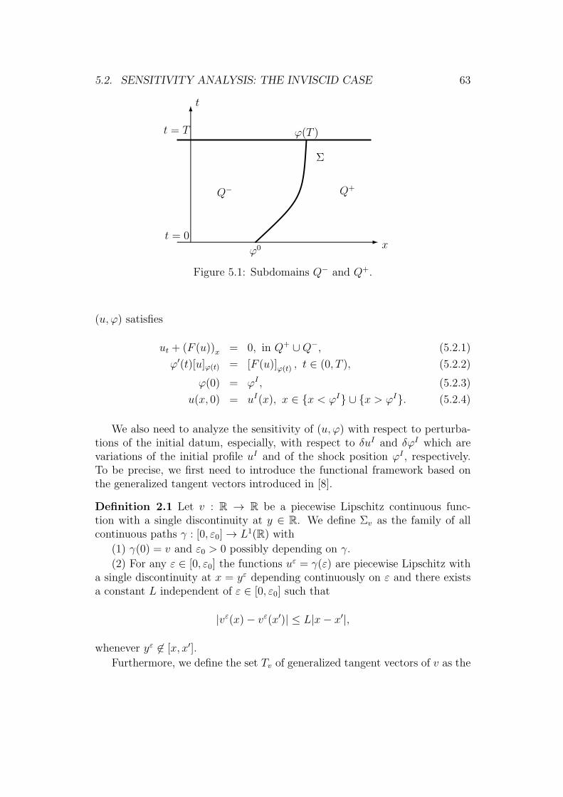
5.2. SENSITIVITY ANALYSIS: THE INVISCID CASE 63
t = 0
t = T
t
φ(T )
Q+Q−
Σ
φ0 x
Figure 5.1: Subdomains Q− and Q+.
(u, φ) satisfies
ut + (F (u))x = 0, in Q+ ∪Q−, (5.2.1)
φ′(t)[u]φ(t) = [F (u)]φ(t) , t ∈ (0, T ), (5.2.2)
φ(0) = φI , (5.2.3)
u(x, 0) = uI(x), x ∈ x < φI ∪ x > φI. (5.2.4)
We also need to analyze the sensitivity of (u, φ) with respect to perturba-tions of the initial datum, especially, with respect to δuI and δφI which arevariations of the initial profile uI and of the shock position φI , respectively.To be precise, we first need to introduce the functional framework based onthe generalized tangent vectors introduced in [8].
Definition 2.1 Let v : R → R be a piecewise Lipschitz continuous func-tion with a single discontinuity at y ∈ R. We define Σv as the family of allcontinuous paths γ : [0, ε0] → L1(R) with
(1) γ(0) = v and ε0 > 0 possibly depending on γ.
(2) For any ε ∈ [0, ε0] the functions uε = γ(ε) are piecewise Lipschitz witha single discontinuity at x = yε depending continuously on ε and there existsa constant L independent of ε ∈ [0, ε0] such that
|vε(x)− vε(x′)| ≤ L|x− x′|,
whenever yε ∈ [x, x′].
Furthermore, we define the set Tv of generalized tangent vectors of v as the
64CHAPTER 5. AN APPLICATION TO OPTIMAL CONTROL THEORY
space of (δv, δy) ∈ L1 ×R for which the path γ(δv,δy) given by
γ(δv,δy)(ε) =
v + εδv + [v]yχ[y+εδy,y] if δy < 0,
v + εδv − [v]yχ[y,y+εδy] if δy > 0,
satisfies γ(δv,δy) ∈ Σv.Finally, we define the equivalence relation ∼ defined on Σv by
γ ∼ γ′ if and only if limε→0
∥γ(ε)− γ′(ε)∥L1
ε= 0,
and we say that a path γ ∈ Σv generates the generalized tangent vector(δv, δy) ∈ Tv if γ is equivalent to γ(δv,δy).
Remark 2.1. The path γ(δv,δy) ∈ Σv represents, at first order, the varia-tion of a function v by adding a perturbation function εδv and by shifting thediscontinuity by εδy.
Note that, for a given v (piecewise Lipschitz continuous function with asingle discontinuity at y ∈ R) the associated generalized tangent vectors (δv, δy) ∈Tv are those pairs for which δv is Lipschitz continuous with a single disconti-nuity at x = y.
Now we assume that the initial datum uI is Lipschitz continuous to bothsides of a single discontinuity located at x = φI , and consider a generalizedtangent vector (δuI , δφI) ∈ L1(R) × R. Let uI,ε ∈ ΣuI be a path whichgenerates (δuI , δφI). For sufficiently small ε the solution uε of problem (5.2.1)– (5.2.4) is Lipschitz continuous with a single discontinuity at x = φε(t), forall t ∈ [0, T ]. Thus uε generates the generalized tangent vector (δv, δφ) ∈L1(R)×R. Then it is proved in [9] that (δu, δφ) satisfies the linearized system
(δu)t + (f(u)δu)x = 0, in Q+ ∪Q−; (5.2.5)
(δφ)′(t)[u]φ(t) + δφ(t)(φ′(t)[ux]φ(t) − [f(u)ux]φ(t)
)= [f(u)δu]φ(t) − φ′(t)[δu]φ(t), t ∈ (0, T ), (5.2.6)
δφ(0) = δφI , (5.2.7)
δu(x, 0) = δuI(x), x ∈ x < φI ∪ x > φI. (5.2.8)
Remark 2.2. In this way, we can obtain formally the expansion:
(uε, φε) = (u, φ) + ε(δu, δφ) +O(ε2). (5.2.9)
Unfortunately, this expansion is, in general, not true, as we explained in theintroduction. For instance, suppose that δu is bounded and uε is continuous.
5.2. SENSITIVITY ANALYSIS: THE INVISCID CASE 65
From (5.2.9) we conclude that uε converges to u uniformly, whence u shouldbe continuous too. But this is not true in general. Thus we should assume(u, δu) = (u, δu)(x, x/ε, t), a multi-scale expansion.
Remark 2.3. In Section 3, we shall see that equation (5.2.6) can not be, asexpected, recovered as the viscosity ν tends to zero. Instead, it is changed to
[u]φ(t) δφ′(t) = δφ(t)
(− [ux]φ(t)φ
′(t) + [f(u)ux]φ(t)
)+(− [δu]φ(t)φ
′(t) + [f(u)δu]φ(t)
)+1
σ
([ux]φ(t) −
([w]φ(t)φ
′(t)− [f(u)w]φ(t)) ), (5.2.10)
in which a corrector (the term involving σ) is added. Here w is a function whichwill be constructed by asymptotic expansion and has limits as x → ±φ(t) fort ∈ (0, T ).
5.2.2 Sensitivity in presence of shocks
To study the sensitivity, in the presence of shocks, of J with respect to varia-tions associated with the generalized tangent vector, we define an appropriategeneralization of the Gateaux derivative.
Definition 2.2 (Ref. [8]) Let J : L1(R) → R be a functional and uI ∈ L1(R)be Lipschitz continuous with a discontinuity at x = φI an initial datum forwhich the solution of (5.1.1) satisfies hypothesis (H). J is Gateaux differentiableat uI in a generalized sense if for any generalized tangent vector (δuI , δφI) andany family uI,ε ∈ ΣuI associated to (δuI , δφI) the following limit exists,
δJ = limε→0
J(uI,ε)− J(uI)
ε.
Moreover, it depends only on (uI , φI) and (δuI , δφI), i.e. it does not dependon the particular family uI,ε which generates (δuI , δφI). The limit is the ge-neralized Gateux derivative of J in the direction (δuI , δφI).
Then we have the proposition which characterizes the generalized Gateauxderivative of J in terms of the solution to the associated adjoint system.
Proposition 2.1 Assume that uD is continuous at x = φ(T ). The Gateauxderivative of J can be written as follows:
δJ =
∫x<φI∪x>φI
p(x, 0)δuI(x)dx+ q(0)[uI ]φIδφI ,
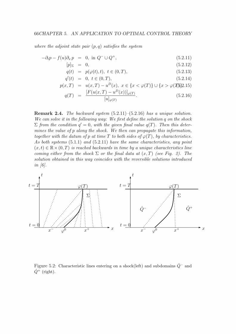
66CHAPTER 5. AN APPLICATION TO OPTIMAL CONTROL THEORY
where the adjoint state pair (p, q) satisfies the system
−∂tp− f(u)∂x p = 0, in Q− ∪Q+, (5.2.11)
[p]Σ = 0, (5.2.12)
q(t) = p(φ(t), t), t ∈ (0, T ), (5.2.13)
q′(t) = 0, t ∈ (0, T ), (5.2.14)
p(x, T ) = u(x, T )− uD(x), x ∈ x < φ(T ) ∪ x > φ(T ),(5.2.15)
q(T ) =[F (u(x, T )− uD(x))]φ(T )
[u]φ(T )
. (5.2.16)
Remark 2.4. The backward system (5.2.11)–(5.2.16) has a unique solution.We can solve it in the following way: We first define the solution q on the shockΣ from the condition q′ = 0, with the given final value q(T ). Then this deter-mines the value of p along the shock. We then can propagate this information,together with the datum of p at time T to both sides of φ(T ), by characteristics.As both systems (5.1.1) and (5.2.11) have the same characteristics, any point(x, t) ∈ R× (0, T ) is reached backwards in time by a unique characteristics linecoming either from the shock Σ or the final data at (x, T ) (see Fig. 2). Thesolution obtained in this way coincides with the reversible solutions introducedin [6].
t = 0
t = T
t
φ(T )
Σ
φ0 xt = 0
t = T
t
φ(T )
Q+Q−
Σ
φ0 xx+x− x+x−
Figure 5.2: Characteristic lines entering on a shock(left) and subdomains Q− and
Q+ (right).
5.2. SENSITIVITY ANALYSIS: THE INVISCID CASE 67
In Figure 2, we have used the following notations:
x− = φ(T )− u−(φ(T ))T, x+ = φ(T )− u+(φ(T ))T,
andQ− = (x, t) ∈ R× (0, T ) such that x < φ(T )− u−(φ(T ))t,
Q+ = (x, t) ∈ R× (0, T ) such that x > φ(T )− u+(φ(T ))t.
Remark 2.5. We shall construct a solution to system (5.2.11)–(5.2.16) in thefollowing manner: We approximate the initial datum (5.1.11) by functions pTnwhich satisfies
pTn are locally Lipschitz continuous, uniformly bounded in BVloc(R) suchthat
pTn (·, T ) → P T (·) = u(·, T )− uD(·) in L1loc(R),
and
pTn (φ(T ), T ) =[F (u(x, T )− uD(x))]φ(T )
[u]φ(T )
.
Then we first take the limit of solutions pν,n of (5.1.10) with initial datapTn , as ν → 0 to obtain the solution pn of
−∂tp− f(u)∂xp = 0, in R× (0, T ), (5.2.17)
p(x, T ) = pTn (x), in R, (5.2.18)
the so-called reversible solution. These solutions can be characterized by thefact that they take the value pn(φ(T ), T ) in the whole region occupied by thecharacteristics that meet the shock. Thus in particular they satisfy the equa-tions (5.2.12)–(5.2.14) and (5.2.16). Moreover, pn → p as n → ∞, and ptakes a constant value in the region occupied by the characteristics that meetthe shock. Note that by construction, this constant is the same for all pn inthis region. Thus this limit solution p coincides with the solution of system(5.2.11)–(5.2.16).
In this chapter, we shall apply the method of matched asymptotic expansionsto justify these convergence results.
5.2.3 The method of alternating descent directions: In-viscid case
We shall present, in this sub-section, the main ideas of the alternating descentmethod which is introduced in [11] for the inviscid Burgers equation. Theclassification of the generalized tangent vectors into two cases is motivated bythe following proposition.
68CHAPTER 5. AN APPLICATION TO OPTIMAL CONTROL THEORY
Proposition 2.2 Assume that we restrict the set of paths in ΣuI to those forwhich the associated generalized tangent vectors (δuI , δφI) ∈ TuI satisfy
δφI = −∫ φI
x− δuIdx+
∫ x+
φI δuIdx
[uI ]φI
. (5.2.19)
Then, the solution (δu, δφ) of problem (5.2.5)–(5.2.8) satisfies δφ(T ) = 0and the general Gateaux derivative of J can be written as follows:
δJ =
∫x<x−∪x>x+
p(x, 0)δuI(x)dx, (5.2.20)
where the adjoint state pair p satisfies the system
−∂tp− f(u)∂x p = 0, in Q− ∪Q+, (5.2.21)
p(x, T ) = u(x, T )− uD(x), x ∈ x < φ(T ) ∪ x > φ(T ).(5.2.22)
Analogously, when considering paths in ΣuI for which the associated gene-ralized tangent vectors (δuI , δφI) ∈ TuI satisfy that δuI = 0, then δu(x, T ) = 0and the general Gateaux derivative of J in the direction (δuI , δφI) can be writ-ten as
δJ = −[F (u(x, T )− uD(x))]φ(T )
[u]φ(T )
[uI ]φIδφI . (5.2.23)
Remark 2.6. Formula (5.2.20) establishes a simplified expression for thegeneralized Gateaux derivative of J when considering directions (δuI , δφI) thatdo not move the shock position at t = T . These directions are characterized byformula (5.2.19) which determines the infinitesimal displacement of the shockposition δφI in terms of the variation of uI to both sides of x = δφI . Note,in particular, that to any value δuI to both sides of the jump φI , a uniqueinfinitesimal translation δφI corresponds of the initial shock position that doesnot move the shock at t = T . We see that formula (5.2.20) holds even if uD isdiscontinuous at x = φ(T ), since we are dealing with a subspace of generalizedtangent vectors satisfying δφ(T ) = 0 and the Gateaux derivative of J , reducedto this subspace, is well defined.
Note also that system (5.2.21)–(5.2.22) does not allow to determine thefunction p outside the region Q−∪ Q+, i.e. in the region under the influence ofthe shock by the characteristic lines emanating from it. However, the value ofp in this region is not required to evaluate the generalized Gateaux derivativein (5.2.20). Analogously, formula (5.2.23) provides a simplified expression ofthe generalized Gateaux derivative of J when considering directions (δuI , δφI)
5.2. SENSITIVITY ANALYSIS: THE INVISCID CASE 69
that uniquely move the shock position at t = T and which correspond to purelytranslating the shock.
Note that the results in Proposition 2.2 suggest the following decompositionof the set of generalized tangent vectors:
TuI = T 1uI ⊕ T 2
uI , (5.2.24)
where T 1uI contains those (δuI , δφI) for which identity (5.2.19) holds, and T 1
uI
the ones for which δuI = 0. Thus this provides two classes of descent directionsfor J at uI . In principle they are not optimal in the sense that they are notthe steepest descent directions but they both have three important properties:
(1) They are both descent directions.(2) They allow to split the design of the profile and the shock location.(3) They are true generalized gradients and therefore keep the structure of
the data without increasing its complexity.When considering generalized tangent vectors belonging to T 1
uI we canchoose as descent direction,
δuI =
−p(x, 0) if x < x−,
− limx→x−, x<x− p(x, 0) if x− < x < φI ,
− limx→x+, x>x+ p(x, 0) if φI < x < x+,
−p(x, 0) if x+ < x,
(5.2.25)
and
δφI = −∫ φI
x− p(x, 0)dx+∫ x+
φI p(x, 0)dx
[u]φI
, (5.2.26)
while for T 2uI a good choice is:
δuI = 0, δφI = [F (u(x, T )− uD(x))]φ(T )
[u(·, T )]φ(T )
[uI ]φI
. (5.2.27)
In (5.2.26) the value of δφI in the interval (x−, x+) does not affect the gene-ralized Gateaux derivative in (5.2.20) under the condition that δφI is chosenexactly as indicated (otherwise the shock would move and this would producean extra term on the derivative of the functional J). We have chosen the sim-plest constant value that preserves the Lipschitz continuity of δuI at x = x−
and x = x+, but not necessarily at x = δφI . Other choices would also providedescent directions for J at uI , but would yield the same Gateaux derivativeaccording to (5.2.20).
70CHAPTER 5. AN APPLICATION TO OPTIMAL CONTROL THEORY
This allows us to define a strategy to obtain descent directions for J at uI
in TuI .
Based upon these studies, an alternating descent method for the optimalcontrol of the Burgers equation can thus be developed, by applying in eachstep of the descent, the following two sub-steps:
1. Use generalized tangent vectors that move the shock to search its optimalplacement.
2. Use generalized tangent vectors to modify the value of the solutionat time t = T to both sides of the discontinuity, leaving the shock locationunchanged.
For more details, we refer the reader to [11], and a number of numericalexperiments show that this method is much more robust and efficient than theusual ones.
In this chapter, motivated by the strategy for obtaining descent directionsfor J in the inviscid case, we will carry out, in Section 5, this procedure forviscous conservation laws provided that the parameter ν is sufficiently small.
We now turn to discuss the existence of minimizers of the functional J ,depending on a small parameter that comes from the solutions to the viscousproblems, over suitable admissible set and their limit as the small parametertends to zero. Let us now introduce the set of admissible initial data Uad ⊂L1(R), which is
Uad = f ∈ L∞(R) | supp(f) ⊂ K, ∥f∥L∞(R)) ≤ C, (5.2.28)
where K ⊂ R is a bounded interval and C > 0 a constant. We shall see laterthis choice guarantees the existence of minimizers for the following optimiza-tion problem:Find uI,min ∈ Uad such that
J(uI,min) = minuI∈Uad
J(uI). (5.2.29)
To make the dependence on the viscosity parameter ν more explicit the func-tional J will be denoted by Jν , although its definition is the same as that ofJ . Similarly we now consider the same minimization problem for the viscousmodel (5.1.4):Find uI,min ∈ Uad such that
Jν(uI,min) = min
uI∈Uad
Jν(uI). (5.2.30)
For the existence of minimizers of the functionals J and Jν , and the conclu-sion that the minimizers of the viscous problem (ν > 0) converge to a minimizer
5.2. SENSITIVITY ANALYSIS: THE INVISCID CASE 71
of the inviscid problem as the viscosity goes to zero, we refer to a recent work[12] for the vanishing viscosity method for the inviscid Burgers equation. Inthat paper, the following theorems are proved.
Theorem 5.2.1 (Existence of Minimizers) Assume that Uad is defined in (5.2.28)and uD ∈ L2(R). Then the minimization problem (5.2.29) and (5.2.30) haveat least one minimizer uI,min ∈ Uad.
Theorem 5.2.2 Any accumulation point as ν → 0 of uI,minν , the minimizers
of (5.2.30), with respect to the weak topology in L2, is a minimizer of thecontinuous problem (5.2.29).
Note that for any positive ν solutions δu, p of equations (5.1.6) and (5.1.10)are smooth, thus the Gateaux derivative of the functional J is as follows
δJ = < δJ(uI), δuI > =
∫Rp(x, 0)δuI(x)dx, (5.2.31)
where the adjoint state p = pν is the solution to (5.1.10) with initial datump(x, T ) = u(x, T )− uD.
Unlike in the inviscid one, the adjoint state now has only one component.Indeed, there is no adjoint shock variable since the state does not presentshocks. Similarly, the derivative of J has also only one term. According tothis, the straightforward application of a gradient method for the optimizationof J would lead, in each step of the iteration, to make use of the variationpointing in the direction
δuI = −p(x, 0), (5.2.32)
where p = pν is the solution to the viscous dual problem. So the alternatingmethod is considerably simplified. But, when processing this way, we wouldnot be exploiting the possibilities that the alternate descent method provides.Therefore, we take into account the effects of possible infinitesimal perturba-tions of initial datum and also infinitesimal translations, and use variations ofthe form
uIε(x) = uIε(x+ εδφI) + εδuIε(x), (5.2.33)
where, φI stands for a reference point on the profile of uI , not necessary apoint of discontinuity. When uI has a point of discontinuity, φI could be itslocation and δφI an infinitesimal variation of it. However φI could also beanother singular point on the profile of uI , as, for instance, an extremal point
72CHAPTER 5. AN APPLICATION TO OPTIMAL CONTROL THEORY
or a point where the gradient of uI is large, namely a smeared discontinuity.By a Taylor expansion, (5.2.33) can be rewritten in the following form
uIε(x) = uI(x) + ε(δφIuIx(x) + δuI(x)
)+O(ε2). (5.2.34)
This indicates that the result of these combined variations (δuI , δφI) is equi-valent to a classical variation in the direction of δφIuIx+ δu
I . We find that theeffect of a small δφI can be amplified by a large gradient δuI .
As we will see in the next section, (5.2.33) and (5.2.34) give us some hintson how to construct outer expansions that include the effects of possible infi-nitesimal perturbations of initial datum and infinitesimal translations.
5.3 Matched asymptotic expansions and ap-
proximate solutions
In this section, we are going to apply the method of matched asymptoticexpansions to construct inner and outer expansions. Then we get the ap-proximate solutions by a suitable combination of them. Firstly, we derive theouter expansions. For the purpose of sensitivity analysis of the states of thesystem, we add infinitesimal perturbations to the initial datum and infinite-simal translations to the shock position, and make use of Taylor expansions.These operations make it possible to derive the equations for the shock andits variation.
Let v = δu, ψ = δφ for simplicity. We consider asymptotic expansions ofsolutions to the following systems.
ut + (F (u))x = νuxx, in R× (0, T ), (5.3.1)
u|t=0 = gε, (5.3.2)
vt + (f(u)v)x = νvxx, in R× (0, T ), (5.3.3)
v|t=0 = hε, (5.3.4)
−pt − f(u)px = νpxx, in R× (0, T ), (5.3.5)
p|t=T = pTn,ε. (5.3.6)
Equation (5.3.1) is the usual conservation law with viscosity, (5.3.3) is itslinearized equation, and (5.3.5) is the dual equation of (5.3.3).
We make the following assumptions:
5.3. MATCHEDASYMPTOTIC EXPANSIONS ANDAPPROXIMATE SOLUTIONS73
Assumptions. A1)
The function F is smooth. (5.3.7)
A2) Let n ∈ N. g0, h0 ∈ L1(R) ∩ L∞(R), g0x ∈ L1(R) and pTn ∈ L1(R) ∩Liploc(R) ∩ L∞(R). g0x, h0 have only a shock at φI , respectively. There existsmooth functions gε, hε, pTn,ε ∈ C∞
0 (R), such that
gε, hε, pTn,ε → g0, h0, pTn (5.3.8)
in L2(R) as ε → 0, respectively. Moreover, we assume that pTn is boundedsequence in BV loc(R) such that as n→ ∞,
pTn → pT in L1loc(R). (5.3.9)
A3) Assume further that Oleinik’s one-sided Lipschitz condition (OSLC)is satisfied, i.e.
(f(u(x, t))− f(u(y, t))) (x− y) ≤ α(t)(x− y)2 (5.3.10)
for almost every x, y ∈ R and t ∈ (0, T ), where α ∈ L1(0, T ).
5.3.1 Outer expansions
An outer expansion is valid outside the interfacial (or quasi-shock) region, itis a series of the following form
η = η(x, t, ν) = η0(x, t) + ν η1(x, t) + ν2 η2(x, t) + · · · , (5.3.11)
or
η = η(x, t, ν) = η0(x, t) + ν η1(x, t) + ν2 η2(x, t) + · · · , (5.3.12)
where η, η0, η0, η1, η
1, · · · depend on variables t, x (but, do not depend onfast variable rν) and will be replaced by u, u0, u
0, u1, u1, · · · , respectively.
So do the initial data h, g, pTn . Hereafter, we use · · · to denote the remainderwhich has higher order of the small parameter ν, thus can be omitted.
Step 1. Outer expansions of u. We start with the construction ofouter expansion of u. The following conventions will apply throughout thissubsection: ui, uij denote a function depending on i and i, j, respectively, wherethe i, j are non-negative integers. The k-th power of ui is denoted by (ui)k.However, if ν is a parameter, νi still stands for the i-th power of ν.
74CHAPTER 5. AN APPLICATION TO OPTIMAL CONTROL THEORY
We now expand the initial data as follows
hε = h0(x) + εh1(x) + ε2h2(x) + · · · , (5.3.13)
pTn,ε = pTn0(x) + εpTn1(x) + ε2pTn2(x) + · · · , (5.3.14)
and the nonlinear terms as
F (η) = F (η0) + νf(η0)η1 + ν2(f(η0)η2 +
1
2f(η0)(η1)
2
)+ · · · ,(5.3.15)
f(η) = f(η0) + νf ′(η0)η1 + ν2(f ′(η0)η2 +
1
2f ′′(η0)(η1)
2
)+ · · · .(5.3.16)
However, the initial datum gε will be expanded in a special manner.In order to analyze the sensitivity of the states with respect to perturbations
of the initial data and the shock position, we construct the outer expansionsin the following way: It is easy to see that the solution u to equation (5.3.1)with (5.3.13) depends on two parameters ν, ε, so we write
u = u(x, t; ν, ε),
and define
xε = x− ε(ν)ψ(t), (5.3.17)
where ε = ε(ν) is a function to be determined. Then making a transformationof variable x→ xε, we obtain a new function
u = u(xε, t; ν, ε) := u(xε + ε(ν)ψ(t), t; ν, ε) = u(x, t; ν, ε).
For the initial data, we make the same transformation of variable, i.e.(5.3.17) with t = 0 , and have
gε(x) = g0(xε) + εg1(xε) + ε2g2(xε) + · · · . (5.3.18)
Here, we defined gi(xε) = gi(xε + εψ(0)) with i = 0, 1, 2.
In order to get the outer expansion of u in the form (5.3.11), we need to doit in two steps. Firstly we expand u(xε, t; ν, ε) in terms of ε and (η, t) = (xε, t)(we now regard xε as an independent variable) as follows
u = u0 + εu1 + ε2u2 + · · · , (5.3.19)
where ui = ui(xε, t; ν), for i = 0, 1, 2, · · · , and we find, by testing differentansatze, that in order to get asymptotic expansions there must hold
ε = σν. (5.3.20)
5.3. MATCHEDASYMPTOTIC EXPANSIONS ANDAPPROXIMATE SOLUTIONS75
Secondly we expand ui in terms of ν and (x, t) as follows. For i = 0, invoking(5.3.17), by Taylor expansions and (5.3.20), one has
u0(xε, t; ν) = u00(xε, t) + νu01(xε, t) + ν2u02(xε, t) + · · ·
= u00(x, t) + u00,x(x, t)εψ +1
2u00,xx(x, t)(εψ)
2 + ν(u01(x, t) + u01,x(x, t)εψ
)+ ν2u02(x, t) + · · ·
= u00(x, t) + ν(u00,x(x, t)σψ + u01(x, t)
)+ ν2
(1
2u00,xx(x, t)(σψ)
2 + u01,x(x, t)σψ + u02(x, t)
)+ · · · .(5.3.21)
In a similar manner, we obtain, for i = 1, 2, that
u1(xε, t; ν) = u10(xε, t) + νu11(xε, t) + · · ·= u10(x, t) + ν
(u10,x(x, t)σψ + u11(x, t)
)+ · · · , (5.3.22)
and
u2(xε, t; ν) = u20(xε, t) + · · · = u20(x, t) + · · · . (5.3.23)
Therefore, from (5.3.19) – (5.3.23) we get an ansatz for u as follows
u = u0 + νu1 + ν2u2, (5.3.24)
here, u0, u1 and u2 are defined by
u0 = u00, (5.3.25)
u1 = u01 + σu10, (5.3.26)
u2 = u02 + σu11 + σ2u20. (5.3.27)
Straightforward computations show that (5.3.1) can be written in terms ofui and ε as
0 = ut + (F (u))x − νuxx
= u0t + (F (u0))x − νu0xx + ε(u1t +
(f(u0)u1
)x− νu1xx
)+ ε2
(u2t + (f(u0)u2 +
f ′(u0)
2(u1)2)x − νu1xx
)+ · · · . (5.3.28)
Inserting (5.3.24) into (5.3.28), recalling ε = σν, then equating the coefficientsof νk (where k = 0, 1, 2) on both sides of the resulting equation, we thus obtain
ν0 : (u0)t + (F (u0))x = 0, (5.3.29)
ν1 : (u1)t + (f(u0)u1)x = R, (5.3.30)
ν2 : (u2)t + (f(u0)u2)x = R1, (5.3.31)
76CHAPTER 5. AN APPLICATION TO OPTIMAL CONTROL THEORY
where R and R1 are functions defined by
R := u0,xx − σ(u0,xψ
′ + ((u0,x)t + (f(u0)u0,x)x)ψ)
and
R1 :=
(1
2u00,xσψ + u01
)xx
−(1
2u00,xx(σψ)
2 + u01,xσψ
)t
− σ(u10,xσψ
)t
−(f(u00)
(1
2u00,xx(σψ)
2 + u01,xσψ
)+
1
2f ′(u00)(u
00,xσψ + u01)
2
)x
−σ(f(u00)u
10,xσψ + f ′(u00)(u
00,xσψ + u01)u
10
)x+ σ(u10)xx − σ2
(1
2f ′(u00)(u
10)
2
)x
=
(1
2u0,xσψ + u1
)xx
−(1
2u0,xx(σψ)
2 + u1,xσψ
)t
−(f(u0)
(1
2u0,xx(σψ)
2 + u1,xσψ
)+
1
2f ′(u0)(u0,xσψ + u1)
2
)x
(5.3.32)
from which we see that R, R1 depend on constant σ and functions ψ, u0 andu1.
We now consider the expansion of the initial data. By using again Taylorexpansions, (5.3.18) can be rewritten as
gε(x) = g0(x) + σν (ψ(0)g′0(x) + g1(x))
+σ2ν2(1
2ψ(0)2g′′0(x) + ψ(0)g1(x) + g2(x)
)+ · · · . (5.3.33)
Thus this expansion suggests us to choose the initial data of ui (i = 0, 1, 2) asfollows
u0|t=0 = g0, (5.3.34)
u1|t=0 = g1, (5.3.35)
u2|t=0 = g2. (5.3.36)
Here, g0, g1, g2 are defined by
g0 = g0, (5.3.37)
g1 = σ (ψ(0)g′0 + δg0) , (5.3.38)
g2 = σ2
(1
2ψ(0)2g′′0 + ψ(0)g1(x) + g2(x)
). (5.3.39)
From (5.3.38) it follows that νg1 is just the second term in (5.2.34). So theexpansion of gε obtained here coincides with the one carried out formally in(5.2.34) in Section 2.
5.3. MATCHEDASYMPTOTIC EXPANSIONS ANDAPPROXIMATE SOLUTIONS77
To solve the equations (5.3.29)–(5.3.31) with initial data (5.3.34)–(5.3.36),we need to get the equations for φ and ψ. So their solvability will be left tosub-section 3.3, where the interface equations will be derived.
Step 2. Outer expansions of v. Now we turn to derive the outer ex-pansions for v. It is not necessary to take into account again the effects ofinfinitesimal perturbations of the initial datum and infinitesimal translationsof the shock position, since we have had, in hand, the equations for shock andits perturbation. We can construct directly an ansatz for v, that has the sameform of (5.3.24), as follows
v = v0 + νv1 + ν2v2. (5.3.40)
Similarly, from equation (5.3.3) we then have
ν0 : (v0)t + (f(u0)v0)x = 0, (5.3.41)
ν1 : (v1)t + (f(u0)v1)x = δ1, (5.3.42)
ν2 : (v2)t + (f(u0)v2)x = δ2, (5.3.43)
and the initial data are
v0|t=0 = h0, (5.3.44)
v1|t=0 = h1, (5.3.45)
v2|t=0 = h2. (5.3.46)
Here δ1, δ2 are given by
δ1 = (v0)xx − (f ′(u0)u1v0)x ,
δ2 = (v1)xx −(f ′(u0)u2v0 +
1
2f ′′(u0)(u1)
2v0
)x
. (5.3.47)
By solving these problems (which are initial value problems of transportequations with discontinuous coefficients, for the well-posedness we refer toe.g. [6]), we then construct v0, v1, v2 which are smooth up to the shock.
Step 3. Outer expansions of p. To get the outer expansions for p werepeat again the procedure performed for v, similarly, from equation (5.3.5)we then have
ν0 : (p0)t + f(u0)(p0)x = 0, (5.3.48)
ν1 : (p1)t + f(u0)(p1)x = β1, (5.3.49)
ν2 : (p2)t + f(u0)(p2)x = β2, (5.3.50)
78CHAPTER 5. AN APPLICATION TO OPTIMAL CONTROL THEORY
and the initial data are
p0|t=0 = pT0 , (5.3.51)
p1|t=0 = pT1 , (5.3.52)
p2|t=0 = pT2 . (5.3.53)
Here β1, β2 are given by
β1 = − (f ′(u0)u1(p0)x + (p0)xx) , (5.3.54)
β2 = −(f ′(u0)u1(p1)x +
(f ′(u0)u2 +
f ′′(u0)
2(u1)
2
)(p0)x + (p1)xx
).(5.3.55)
Thus we first solve p0, then insert p0 into equations p1 and p2, from theresulting linear equations we then can obtain p1 and p2.
We are now going to discuss the solvability of the problems (5.3.29) –(5.3.36). There are five unknowns, i.e. ui (i = 0, 1, 2), φ and ψ, but only threeequations. So, to form a complete system, as the first step, we need to findthe equations that φ and ψ satisfy.
5.3.2 Derivation of the interface equations
In this sub-section we shall derive the interface equations from the outer ex-pansions of u, this derivation is based upon an important observation that thevalues of outer expansions tend to those at the shock φ(t), as the thicknessν of the quasi-shock region goes to zero. This is different from the usual waythat one derives such equations from inner expansions, see, e.g. [14, 16]. Oneadvantage of this approach is that we can overcome the difficulty/limitationcaused by the algebraically growth, as rν → ∞, which is required by the mat-ching conditions, i.e. (5.3.73), of the second term i.e. u1 of inner expansionof u, so how to define the jump (e.g. u1(∞, t) − u1(−∞, t), but u1(±∞, t)may not exsist) of the terms like u1, of the inner expansion of u? We cannotdefine it in a usual way, some restrictions must be imposed, for instance, addan assumption that ∂xu0(φ(t)± 0, t) = 0 for u1.
Assume that the limits of ui (or its derivatives) exist for any t ∈ [0, T ],from the left and right side of the shock, i.e.
∂kxu0(φ(t)± 0, t), k = 0, 1, and u1(φ(t)± 0, t), exist.
First of all, we derive the equation for the shock, and invoke equation(5.3.29) with initial datum (5.3.34) which is just a Cauchy problem for theunknown u0. From the standard theory it then follows that
φ′ [u0]φ(t) = [F (u0)]φ(t), (5.3.56)
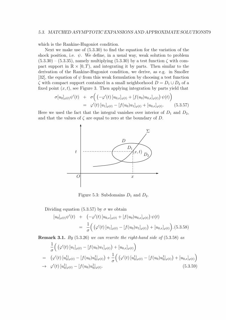
5.3. MATCHEDASYMPTOTIC EXPANSIONS ANDAPPROXIMATE SOLUTIONS79
which is the Rankine-Hugoniot condition.Next we make use of (5.3.30) to find the equation for the variation of the
shock position, i.e. ψ. We define, in a usual way, weak solution to problem(5.3.30) – (5.3.35), namely multiplying (5.3.30) by a test function ζ with com-pact support in R × [0, T ), and integrating it by parts. Then similar to thederivation of the Rankine-Hugoniot condition, we derive, as e.g. in Smoller[32], the equation of ψ from this weak formulation by choosing a test functionζ with compact support contained in a small neighborhood D = D1 ∪D2 of afixed point (x, t), see Figure 3. Then applying integration by parts yield that
σ[u0]φ(t)ψ′(t) + σ
( (−φ′(t) [u0,x]φ(t) + [f(u0)u0,x]φ(t)
)ψ(t)
)= φ′(t) [u1]φ(t) − [f(u0)u1]φ(t) + [u0,x]φ(t). (5.3.57)
Here we used the fact that the integral vanishes over interior of D1 and D2,and that the values of ζ are equal to zero at the boundary of D.
x
t
O
(x, t)D1
D2
Σ
D
Figure 5.3: Subdomains D1 and D2.
Dividing equation (5.3.57) by σ we obtain
[u0]φ(t)ψ′(t) +
(−φ′(t) [u0,x]φ(t) + [f(u0)u0,x]φ(t)
)ψ(t)
=1
σ
( (φ′(t) [u1]φ(t) − [f(u0)u1]φ(t)
)+ [u0,x]φ(t)
).(5.3.58)
Remark 3.1. By (5.3.26) we can rewrite the right-hand side of (5.3.58) as
1
σ
( (φ′(t) [u1]φ(t) − [f(u0)u1]φ(t)
)+ [u0,x]φ(t)
)=
(φ′(t) [u10]φ(t) − [f(u0)u
10]φ(t)
)+
1
σ
( (φ′(t) [u10]φ(t) − [f(u0)u
10]φ(t)
)+ [u0,x]φ(t)
)→ φ′(t) [u10]φ(t) − [f(u0)u
10]φ(t). (5.3.59)
80CHAPTER 5. AN APPLICATION TO OPTIMAL CONTROL THEORY
Thus we see that if f(u) = u, equation (5.3.58) converges to the one derivedin [8].
We turn back to solvability of equation (5.3.58). To this end we need todetermine a priori the quantity [u1]φ(t). Invoking outer expansions of uν andvν , noting that vν is the variation of uν , we have two expansions of uν , whichare valid up to the shock,
u(x, t; ν, σν) =: uν = u0 + νu1 + · · · (5.3.60)
= u+ νvν + · · · = u+ νv0 + · · · . (5.3.61)
Here u is believed to be the entropy solution to problem (5.1.1)–(5.1.2). So itis natural to assume that u0 = u, whence u1 = v0. Thus, there must hold
limx→φ(t)
u1(x, t) = limx→φ(t)
v0(x, t) = v0(φ(t), t)
for any t ∈ [0, T ].Therefore, we can write [u1]φ(t) in terms of [v0]φ(t). From (5.3.56) we get
φ = φ(t) and insert it into (5.3.58). Hence from (5.3.58) one solves (5.3.58)and gets ψ. Furthermore, we can solve u0 from equation (5.3.29) with (5.3.34)which form a Riemann problem. Once u0 is obtained, we see that the righthand side of (5.3.30) and (5.3.31), namely R, R1 are also known quantities,thus problem (5.3.30) with (5.3.35) and problem (5.3.31) with (5.3.36) arelinear in u1, u2 respectively, and can be solved easily to get u1, u2.
Combining the results obtained in sub-sections 3.1 and 3.2, we then com-plete the construction of outer expansions of u, v and p. We also find that thefirst term v0 of the outer expansion of v(x, t; ν, ε) can be expected to solve
(v0)t + (f(u0)v0)x = 0, in Q+ ∪Q−; (5.3.62)
[u0]φ(t)ψ′(t) +
(−φ′(t) [u0,x]φ(t) + [f(u0)u0,x]φ(t)
)ψ(t)
=1
σ
( (φ′(t) [v0]φ(t) − [f(u0)v0]φ(t)
)+ [u0,x]φ(t)
),(5.3.63)
ψ(0) = δφI , (5.3.64)
v0(x, 0) = vI(x), x ∈ x < φI ∪ x > φI. (5.3.65)
Note that (5.2.6) is replaced by (5.3.63).
Remark 3.2. By the method of characteristics, we solve u1 from problem(5.3.30), (5.3.35), and write it as
u1(x, t) = u1(x(0), 0)
∫ t
0
R(x, s) · exp(∫ s
t
(f(u0(x, τ)))xdτ
)ds,
5.3. MATCHEDASYMPTOTIC EXPANSIONS ANDAPPROXIMATE SOLUTIONS81
for (x, t) ∈ Q+ ∪Q−, and ψ from (5.3.58). Thus we see that ψ, u1 depend onthe parameter σ. On the other hand, under assumption that ψ depends on σ,checking the construction we find that functions u01 and u
10 are still independent
of σ. Therefore, by formula (5.3.26) we assert that
u01 = u1(x, t; σ)|σ=0 = u1(x(0), 0)
∫ t
0
u0,xx(x, s) exp
(∫ s
t
(f(u0(x, τ)))xdτ
)ds,
whence
u10 =1
σ(u1 − u01). (5.3.66)
Note that u01 is the second term of outer expansions suppose that there is noperturbation of the initial datum. It is possible that the right hand side of(5.3.66) is independent of σ.
5.3.3 Inner expansions
An inner expansion is the one that is valid inside the interfacial region, whichcan be written as a series consisting of terms in fast variable r = rν and time t
η = η(rν , t, ν) = η0(r, t) + νη1(r, t) + ν2η2(r, t) + · · · ,
here η, η0, η1, · · · will be replaced by u, u0, u1, · · · , v, v0, v1, · · · andp, p0, p1, · · · , respectively.
The nonlinear terms can be expanded as
F (η) = F (η0) + νf(η0)η1 + ν2(f(η0)η2 +
1
2f(η0)η
21
)+ · · · , (5.3.67)
f(η) = f(η0) + νf ′(η0)η1 + ν2(f ′(η0)η2 +
1
2f ′′(η0)η
21
)+ · · · . (5.3.68)
In what follows, for implicity, we use the notation
h′ =∂
∂rνh
for a function h in fast variable. Then we have
∂h
∂dν=
1
νh′,
∂2h
∂dν2 =
1
ν2h′′.
82CHAPTER 5. AN APPLICATION TO OPTIMAL CONTROL THEORY
Therefore, we have
ν−1 : u′′0 + φu′0 − (F (u0))′ = 0, (5.3.69)
ν0 : u′′1 + φu′1 − (f(u0)u1)′ = −σψu′0 + u0t, (5.3.70)
ν1 : u′′2 + φu′2 − (f(u0)u2)′ = −σψu′1
(f ′(u0)
2u21
)′
+ u1t. (5.3.71)
Then we use the matching conditions which make the inner and outer expan-sions coincide asymptotically in an intermediate region, say M. Over thisregion, there holds
u0(rν , t)+νu1(rν , t)+ν2u2(rν , t) = u0(x, t)+νu1(x, t)+ν
2u2(x, t)+O(ν3), inM.
By definition, we can rewrite x = ν(rν + σψ(t)) + φ(t). Then using Taylorexpansions we can obtain the matching conditions in the following form
u0(rν , t) = u0(φ(t)± 0, t) + o(1), (5.3.72)
u1(rν , t) = u1(φ(t)± 0, t) + (rν + σψ)∂xu0(φ(t)± 0, t) + o(1),(5.3.73)
u2(rν , t) = u2(φ(t)± 0, t) + (rν + σψ)∂xu1(φ(t)± 0, t)
+(rν + σψ)2
2∂2xu0(φ(t)± 0, t) + o(1), (5.3.74)
for more details, we refer, e.g. to the book by Fife [14]. Later we will chooseo(1) = exp(−cξ2), where c is a fixed positive number.
Therefore the problems (5.3.69) – (5.3.71) with corresponding boundaryconditions (5.3.72) – (5.3.74), which are boundary value problems of ordinarydifferential equations of second order, have a unique solution, respectively,provided the orthogonality conditions are met:∫ ∞
−∞(−σψu′0 + u0t)p
∗dr = 0 and
∫ ∞
−∞
(−σψu′1
(f ′(u0)
2u21
)′
+ u1t
)p∗dr = 0(5.3.75)
where p∗ satisfied L∗(p∗) = 0, and L∗ is the adjoint operator of L which isdefined by
L(u1) = u′′1 + φu′1 − (f(u0)u1)′.
We thus obtain u0, u1, u2.
Straightforward computations yield the equations for the inner expansionof v
ν−1 : v′′0 + φv′0 − (f(u0)v0)′ = 0, (5.3.76)
ν0 : v′′1 + φv′1 − (f(u0)v1)′ = f1, (5.3.77)
ν1 : v′′2 + φv′2 − (f(u0)v2)′ = f2, (5.3.78)
5.3. MATCHEDASYMPTOTIC EXPANSIONS ANDAPPROXIMATE SOLUTIONS83
where f1 and f2 are defined by
f1 = v0t − σψv′0 + (f ′(u0)u1v0)′, (5.3.79)
f2 = v1t − σψv′1 +
(f ′(u0)u1v1 +
(f ′(u0)u2 +
1
2f ′′(u0)u
21
)v0
)′
.(5.3.80)
Using the matching conditions
v0(rν , t) = v0(φ(t)± 0, t) + o(1), (5.3.81)
v1(rν , t) = v1(φ(t)± 0, t) + (rν + σψ)∂xv0(φ(t)± 0, t) + o(1),(5.3.82)
v2(rν , t) = v2(φ(t)± 0, t) + (rν + σψ)∂xv1(φ(t)± 0, t)
+(rν + σψ)2
2∂2xv0(φ(t)± 0, t) + o(1), (5.3.83)
Solving problems (5.3.76) – (5.3.78) with suitable orthogonality conditions andalso boundary conditions (5.3.81) – (5.3.83), we then obtain v0, v1, v2.
Finally we construct the inner expansion of p, the first three terms of itcan be obtained by solving the following equations
ν−1 : p′′0 − φp′0 + f(u0)p′0 = 0, (5.3.84)
ν0 : p′′1 − φp′1 + f(u0)p′1 = f3, (5.3.85)
ν1 : p′′2 − φp′2 + f(u0)p′2 = f4, (5.3.86)
where f3 and f4 are defined by
f3 = ψp′0 − p0t − f ′(u0)u1p′0, (5.3.87)
f4 = ψp′1 − p1t − f ′(u0)u1v1 −(f ′(u0)u2 +
1
2f ′′(u0)u
21
)p′0. (5.3.88)
One can easily find that equations satisfied by pi (i = 0, 1, 2), namely (5.3.84)– (5.3.86) are just the dual ones of those satisfied by vi, i.e. (5.3.76) – (5.3.78).
From the following matching conditions
p0(rν , t) = p0(φ(t)± 0, t) + o(1), (5.3.89)
p1(rν , t) = p1(φ(t)± 0, t) + (rν + σψ)∂xp0(φ(t)± 0, t) + o(1),(5.3.90)
p2(rν , t) = p2(φ(t)± 0, t) + (rν + σψ)∂xp1(φ(t)± 0, t)
+(rν + σψ)2
2∂2xp0(φ(t)± 0, t) + o(1), (5.3.91)
we solve uniquely, under suitable orthogonality conditions, equations (5.3.84)– (5.3.86) and get p0, p1, p2.
84CHAPTER 5. AN APPLICATION TO OPTIMAL CONTROL THEORY
Therefore, we have constructed the inner and outer expansions up to ν2,for u, v, p respectively, which can be written as follows
U2(x, t) = u0 + νu1 + ν2u2, (5.3.92)
U2(r, t) = u0 + νu1 + ν2u2. (5.3.93)
V2(x, t) = v0 + νv1 + ν2v2, (5.3.94)
V2(r, t) = v0 + νv1 + ν2v2. (5.3.95)
P2(x, t) = p0 + νp1 + ν2p2, (5.3.96)
P2(r, t) = p0 + νp1 + ν2p2. (5.3.97)
5.3.4 Approximate solutions
In this subsection we shall use a suitable cut-off function to combine togetherthe outer and inner expansions derived in sub-sections 3.1, 3.3 and 3.4, whencethe approximate solutions will be constructed.
We define a function χ = χ(ξ) : R → R+ which is smooth such that
χ(ξ) =
1 if |ξ| ≤ 1,
0 if |ξ| ≥ 2,(5.3.98)
and 0 ≤ χ(ξ) ≤ 1 if ξ ∈ [1, 2]. And let
χν(x, t) = χ(ν1−γrν), (5.3.99)
which is easily seen from Figure 4 that
supp(χν) ⊂ [0, 2νγ], supp(χ′ν), supp(χ
′′ν) ⊂ [νγ, 2νγ].
From the expansions (5.3.92) and (5.3.93), (5.3.94) and (5.3.95) and (5.3.96)and (5.3.97), we are in a position to construct, respectively, the approximatesolutions U ν
2 , Vν2 and P ν
2 as follows
U ν2 (x, t) = χν(x, t)U2(rν , t) + (1− χν(x, t))U2(x, t), (5.3.100)
V ν2 (x, t) = χν(x, t)V2(rν , t) + (1− χν(x, t))V2(x, t), (5.3.101)
P ν2 (x, t) = χν(x, t)P2(rν , t) + (1− χν(x, t))P2(x, t). (5.3.102)
By definition, we find easily that if (x, t) is sufficiently close to the quasi-shockx = φ(t), then χν(x, t) = 1, thus the approximate solution U ν
2 is equal to innerexpansion U2, namely
U ν2 (x, t) = U2(rν , t),
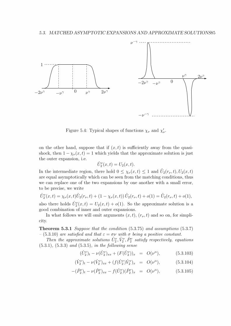
5.3. MATCHEDASYMPTOTIC EXPANSIONS ANDAPPROXIMATE SOLUTIONS85
νγ 2νγ0
1
−νγ−2νγ
νγ 2νγ
0−νγ−2νγ
ν−γ
−ν−γ
Figure 5.4: Typical shapes of functions χν and χ′ν .
on the other hand, suppose that if (x, t) is sufficiently away from the quasi-shock, then 1−χν(x, t) = 1 which yields that the approximate solution is justthe outer expansion, i.e.
U ν2 (x, t) = U2(x, t).
In the intermediate region, there hold 0 ≤ χν(x, t) ≤ 1 and U2(rν , t), U2(x, t)are equal asymptotically which can be seen from the matching conditions, thuswe can replace one of the two expansions by one another with a small error,to be precise, we write
U ν2 (x, t) = χν(x, t)U2(rν , t) + (1− χν(x, t)) U2(rν , t) + o(1) = U2(rν , t) + o(1),
also there holds U ν2 (x, t) = U2(x, t) + o(1). So the approximate solution is a
good combination of inner and outer expansions.In what follows we will omit arguments (x, t), (rν , t) and so on, for simpli-
city.
Theorem 5.3.1 Suppose that the condition (5.3.75) and assumptions (5.3.7)– (5.3.10) are satisfied and that ε = σν with σ being a positive constant.
Then the approximate solutions U ν2 , V
ν2 , P
ν2 satisfy respectively, equations
(5.3.1), (5.3.3) and (5.3.5), in the following sense
(U ν2 )t − ν(U ν
2 )xx + (F (U ν2 ))x = O(να), (5.3.103)
(V ν2 )t − ν(V ν
2 )xx + (f(U ν2 )V
ν2 )x = O(να), (5.3.104)
−(P ν2 )t − ν(P ν
2 )xx − f(U ν2 )(P
ν2 )x = O(να), (5.3.105)
86CHAPTER 5. AN APPLICATION TO OPTIMAL CONTROL THEORY
where α = 3γ − 1 and γ ∈ (13, 1).
5.4 Convergence of the approximate solutions
This section is devoted to the proof of following Theorem 4.1, which consistsof two parts, one is to prove Theorem 3.1 which asserts that the equations aresatisfied asymptotically, and another is to investigate the convergence rate.
Theorem 5.4.1 Suppose that the assumptions in Theorem 3.1 are met. Letu, p be, respectively, the unique entropy solution with only one shock, the re-versible solution to problems (5.1.1) – (5.1.2) and (5.1.8) – (5.1.9), and let vbe the unique solutions to problem (5.3.62) – (5.3.65), such that∫ T
0
∫x =φ(t), t∈[0,T ]
6∑i=1
(|∂ixu(x, t)|2 + |∂ixv(x, t)|2 + |∂ixp(x, t)|2
)dxdt ≤ C.(5.4.1)
Then the solutions (uν , vν) of problems (5.3.1) – (5.3.2) and (5.3.3) – (5.3.4)converge, respectively, to (u, v) in L∞(0, T ;L2(R))×L∞(0, T ;L2(R)), and thefollowing estimates hold
sup0≤t≤T
∥uν(t)− u(t)∥+ sup0≤t≤T
∥vν(t)− v(t)∥ ≤ Cηνη. (5.4.2)
The solution pν,n of problem (5.3.5) – (5.3.6) converges to p in L∞(0, T ;L1loc(R)),
namely,
sup0≤t≤T
∥pν,n(t)− p(t)∥L1loc(R) → 0, (5.4.3)
as first ν → 0, then n → ∞. Moreover, we also have in a sub-domain thefollowing estimate
sup0≤t≤T
∥pν,n − pn∥L∞(Ωh) ≤ Cν → 0, (5.4.4)
as ν → 0. Here η is a constant defined by
η = min
3
2γ,
1 + γ
2
, where γ is the same as in Theorem 3.1, (5.4.5)
and Cη denotes a constant depending only on parameters η. The domain Ωh
is defined, for any positive constant h, by
Ωh = (x, t) ∈ QT | |x− φ(t)| > h.
5.4. CONVERGENCE OF THE APPROXIMATE SOLUTIONS 87
Remark 4.1. Combination of (5.4.4) and a stability theorem of the reversiblesolutions (see Theorem 4.1.10 in Ref. [6])) yields that
sup0≤t≤T
∥pν,n − p∥L∞(Ωh∩[−R,R]) → 0, (5.4.6)
as ν → 0, then n → ∞, where R is any positive constant. This ensures us toselect alternating descent directions.
5.4.1 The equations are satisfied asymptotically
In this sub-section, we are going to prove that the approximate solutionsU ν2 , V
ν2 , P
ν2 satisfy asymptotically, the corresponding equations (5.3.1), (5.3.3)
and (5.3.5) respectively. For simplicity, in this sub-section we omit the super-script ν and write the approximate solutions as U2, V2, P2.
Proof of Theorem 3.1. We divide the proof into three parts.
Part 1. We first investigate the convergence of U2. Straightforward computa-tions yield
(U2)t =dtνγχ′ν
(U2 − U2
)+ χν · (U2)t + (1− χν)(U2)t, (5.4.7)
(U2)x =1
νγχ′ν
(U2 − U2
)+ χν · (U2)x + (1− χν)(U2)x, (5.4.8)
(U2)xx =1
ν2γχ′′ν
(U2 − U2
)+
2
νγχ′ν
(U2 − U2
)x
+χν · (U2)xx + (1− χν)(U2)xx. (5.4.9)
Hereafter, to write the derivatives of U2 in the form, like the first term in theright hand side of (5.4.7), we changed the arguments t, x of U2, V2, P2 to t, d,where d = d(x, t) is defined by
d(x, t) = x− φ(t).
However, risking abuse of notations we still denote U2(d, t), V2(d, t), P2(d, t) byU2, V2, P2 for the sake of simplicity. After such a transformation of arguments,the terms are easier to deal with, as we shall see later on.
Therefore, we find that U2 satisfies
(U2)t − ν (U2)xx + (F (U2))x = I1 + I2 + I3, (5.4.10)
where Ik (k = 1, 2, 3) are the collections of like-terms according to whether ornot their supports are contained in a same sub-domain of R, more precisely,
88CHAPTER 5. AN APPLICATION TO OPTIMAL CONTROL THEORY
they are defined by
I1 = χν
((U2)t − ν(U2)xx + f(U2) · (U2)x
), (5.4.11)
I2 = (1− χν)((U2)t − ν(U2)xx + f(U2)(U2)x
), (5.4.12)
I3 = (U2 − U2)
(dtχ
′ν
νγ− χ′′
ν
ν2γ−1+χ′νf(U2)
νγ
)− 2χ′
ν
νγ−1
(U2 − U2
)x.(5.4.13)
It is easy to see that the support of I1, I2 is, respectively, a subset of[0, 2νγ] and a subset of [νγ,∞), while the support of I3 is a subset of [νγ, 2νγ]∪[−2νγ,−νγ].
Now we turn to estimate I1, I2, I3. Firstly we handle I3. In this case onecan apply the matching conditions (5.3.72) – (5.3.74) and use Taylor expan-sions to obtain
∂lx(U2 − U2)(x, t) = O(1)ν(3−l)γ (5.4.14)
on the domain (x, t) | νγ ≤ |x − φ(t)| ≤ 2 νγ, 0 ≤ t ≤ T and l = 0, 1, 2, 3.From these estimates (5.4.14), which can also be found, e.g. in Goodman andXin [21], the following assertion follows easily that
I3 = O(1)ν2γ as ν → 0. (5.4.15)
Moreover, we have∫R|I3(x, t)|2dx =
∫νγ≤|x−φ(t)|≤2 νγ
|I3(x, t)|2dx ≤ Cν5γ. (5.4.16)
To deal with I1, I2 we rearrange the terms of I1, I2 as follows
I1 = χν
((U2)t − ν(U2)xx + (F (U2))x
)+ χν ·
(f(U2)− f(U2)
)(U2)x,
= I1a + I1b, (5.4.17)
I2 = (1− χν)((U2)t − ν(U2)xx + (F (U2))x
)+ (1− χν)
(f(U2)− f(U2)
)(U2)x,
= I2a + I2b. (5.4.18)
Moreover, I1b can be rewritten as
I1b = χν
∫ 1
0
f ′(sU2 + (1− s)U2)ds · (U2 − U2)(U2)x. (5.4.19)
Note that supp I1b ⊂ (x, t) ∈ QT | |x − φ(t)| ≤ 2 νγ and U2(x, t) = U2(x, t)if (x, t) ∈ QT | |x − φ(t)| ≤ νγ. Therefore, from (5.4.14) and (5.4.19) weobtain
|I1b| =C
ν|(U2 − U2)(U2)
′| = O(ν3γ−1), (5.4.20)
5.4. CONVERGENCE OF THE APPROXIMATE SOLUTIONS 89
where we choose γ > 13so that 3γ − 1 > 0. Recalling the construction of U2,
from equations (5.3.69) – (5.3.71), we can rewrite I1a as
I1a = χν
((U2)t − ν(U2)xx + (F (u0) + νf(u0)u1 + ν2(f(u0)u2 +
1
2f ′(u0)u
21) +Ru)x
)= χν(Ru)x, (5.4.21)
where the remainder Ru is defined by
Ru = F (U2)−(F (u0) + νf(u0)u1 + ν2(f(u0)u2 +
1
2f ′(u0)u
21)
)= O(ν3).
Thus
|I1a| ≤ |(Ru)x| =1
ν|(Ru)
′| = O(ν2). (5.4.22)
In a similar manner, we now handle I2, and rewrite I2b as
I2b = (1− χν)
∫ 1
0
f ′(sU2 + (1− s)U2)ds · (U2 − U2)(U2)x. (5.4.23)
It is easy to see that supp I2b ⊂ |d| ≥ νγ and U2 = U2 if |d| ≥ 2νγ. From thefact that U2 − U2 = χν(U2 − U2) and (5.4.14) it follows that
|I2b| ≤ C χν |(U2 − U2)(U2)x| = O(ν3γ). (5.4.24)
As for I2a, invoking equations (5.3.29) and (5.3.30) we assert that there holds
I2a = (1− χν)((U2)t − ν(U2)xx + (F (u0) + νf(u0)u1 +Ru)x
)= (1− χν)(Ru)x +O(ν2). (5.4.25)
and the remainder Ru is given by
Ru = F (U2)− (F (u0) + νf(u0)u1) = O(ν2),
hence
I2a = O(ν2). (5.4.26)
On the other hand, we have∫R|I1(x, t)|2dx =
∫|x−φ(t)|≤2 νγ
|I1(x, t)|2dx
≤∫|x−φ(t)|≤νγ
|I1a(x, t)|2dx+∫νγ≤|x−φ(t)|≤2 νγ
|I1b(x, t)|2dx
≤ C(ν2∗2+1 + ν6γ−2+γ) ≤ C νγ. (5.4.27)
90CHAPTER 5. AN APPLICATION TO OPTIMAL CONTROL THEORY
Here we used the simple inequalities: 6γ − 2 + γ < 5 and 6γ − 2 > 0 since weassume γ ∈ (1
3, 1).
Similarly, one can obtain∫R|I2(x, t)|2dx =
∫|x−φ(t)|≥νγ
|I2(x, t)|2dx ≤ C(ν2∗2+1 + ν6γ+γ) ≤ C νγ.(5.4.28)
In conclusion, from (5.4.10), (5.4.15), (5.4.20), (5.4.22), (5.4.24) and (5.4.26)we are in a position to assert that U ν
2 satisfies the equation in the followingsense
(U ν2 )t − ν(U ν
2 )xx + (F (U ν2 ))x = O(να),
as ν → 0. Here α = 3γ − 1 and we used the fact that 3γ − 1 < 2γ < 2by assumption γ < 1. Furthermore, from construction we see easily that theinitial data is satisfied asymptotically too.
Part 2. We now turn to investigate the convergence of V2. Similar computa-tions show that V2 can be written in terms of V2, V2 as
(V2)t =dtνγχ′ν
(V2 − V2
)+ χν · (V2)t + (1− χν)(V2)t, (5.4.29)
(V2)x =1
νγχ′ν
(V2 − V2
)+ χν · (V2)x + (1− χν)(V2)x, (5.4.30)
(V2)xx =1
ν2γχ′′ν
(V2 − V2
)+
2
νγχ′ν
(V2 − V2
)x
+χν · (V2)xx + (1− χν)(V2)xx, (5.4.31)
and V2 satisfies the following equation
(V2)t − ν (V2)xx + (f(U2)V2)x = J1 + J2 + J3, (5.4.32)
where Jk (k = 1, 2, 3) are given, according to their supports, by
J1 = χν
((V2)t − ν(V2)xx +
(f(U2)V2
)x
), (5.4.33)
J2 = (1− χν)((V2)t − ν(V2)xx +
(f(U2)V2
)x
), (5.4.34)
J3 =
(dtχ
′ν
νγ− χ′′
ν
ν2γ−1+f(U2)χ
′ν
νγ
)(V2 − V2)−
2χ′ν
νγ−1(V2 − V2)x.(5.4.35)
Since for V2, we also have the same estimate (5.4.14) which is valid for U2,namely we have
∂lx(V2 − V2) = O(1)ν(3−l)γ (5.4.36)
5.4. CONVERGENCE OF THE APPROXIMATE SOLUTIONS 91
on the domain (x, t) | νγ ≤ |x − φ(t)| ≤ 2 νγ, 0 ≤ t ≤ T and l = 0, 1, 2, 3.Thus it follows from (5.4.36) and the uniform boundedness of U2 that
J3 = O(1)ν2γ, as ν → 0. (5.4.37)
The investigation of convergence for J1, J2 is more technically complicatedthan I1, I2. Rewrite J1, J2 as
J1 = χν
((V2)t − ν(V2)xx + (f(U2)V2)x
)+ χν ·
((f(U2)− f(U2)) V2
)x
= J1a + J1b, (5.4.38)
and
J2 = (1− χν)((V2)t − ν(V2)xx + (f(U2)V2)x
)+ (1− χν)
((f(U2)− f(U2)V2
)x
= J2a + J2b. (5.4.39)
We now deal with J1b which can be changed to
J1b = χν
(∫ 1
0
f ′(sU2 + (1− s)U2)ds(U2 − U2) V2
)x
= χν
(∫ 1
0
f ′(sU2) + (1− s)U2)ds V2
)x
(U2 − U2)
+χν
∫ 1
0
f ′(sU2) + (1− s)U2)ds V2
(U2 − U2
)x
= O(ν3γ−1) +O(ν2γ) = O(ν3γ−1), (5.4.40)
here we used that 3γ − 1 < 2γ since γ < 1.Rewriting J1a as
J1a = χν
((V2)t − ν(V2)xx +
((f(u0) + f ′(u0)(νu1 + ν2u2) +
1
2f ′′(u0)(νu1)
2)V2
)x
)+χν(RvV2)x
= χν
(O(ν2) + (RvV2)x
). (5.4.41)
Here, equations (5.3.76) - (5.3.78) were used. And the remainder Rv is
Rv = f(U2)− (f(u0) + f ′(u0)(νu1 + ν2u2) +1
2f ′′(u0)(νu1)
2) = O(ν3)
Therefore, from (5.4.41) one has
J1a = χν
(O(ν2) + (RvV2)x
)= O(ν2). (5.4.42)
92CHAPTER 5. AN APPLICATION TO OPTIMAL CONTROL THEORY
The terms J2a, J2b can be estimated in a similar way and we obtain
J2b = O(ν3γ) +O(ν2γ) = O(ν2γ), (5.4.43)
and
J2a = (1− χν)((V2)t − ν(V2)xx + ((f(u0) + νf ′(u0)u1 +Rv)V2)x
)= (1− χν)
(O(ν2) + (RvV2)x
),
where Rv is given by Rv = f(U2)− (f(u0) + νf ′(u0)u1) = O(ν2). It is easy tosee that
J2a = O(ν2). (5.4.44)
On the other hand, we have the following estimates of integral type∫R|J1(x, t)|2dx =
∫|x−φ(t)|≤2 νγ
|J1(x, t)|2dx
≤∫|x−φ(t)|≤νγ
|J1a(x, t)|2dx+∫νγ≤|x−φ(t)|≤2 νγ
|J1b(x, t)|2dx
≤ C(ν2∗2+1 + ν6γ−2+γ) ≤ C νγ. (5.4.45)
and∫R|J2(x, t)|2dx =
∫|x−φ(t)|≥νγ
|J2(x, t)|2dx ≤ C(ν2∗2+1 + ν4γ+γ) ≤ C νγ.(5.4.46)
Therefore, it follows from (5.4.32), (5.4.37), (5.4.40), (5.4.42), (5.4.43) and(5.4.44) that V ν
2 satisfies the equation in the following sense
(V ν2 )t − ν(V ν
2 )xx + (f(U ν2 )V
ν2 )x = O(ν3γ−1),
as ν → 0. By construction, the initial data is satisfied asymptotically as well.
Part 3. Finally we turn to investigate the convergence of P2. Computationsshow that the derivatives of P2 can be written in terms of P2, P2 as
(P2)t =dtνγχ′ν
(P2 − P2
)+ χν · (P2)t + (1− χν)(P2)t, (5.4.47)
(P2)x =1
νγχ′ν
(P2 − P2
)+ χν · (P2)x + (1− χν)(P2)x, (5.4.48)
(P2)xx =1
ν2γχ′′ν
(P2 − P2
)+
2
νγχ′ν
(P2 − P2
)x
+χν · (P2)xx + (1− χν)(P2)xx, (5.4.49)
5.4. CONVERGENCE OF THE APPROXIMATE SOLUTIONS 93
and P2 satisfies the following equation
−(P2)t − ν (P2)xx − f(U2)(P2)x = K1 +K2 +K3, (5.4.50)
where Ki (i = 1, 2, 3) are given, according to their supports, by
K1 = −χν
((P2)t + ν(P2)xx + f(U2)(P2)x
), (5.4.51)
K2 = −(1− χν)((P2)t + ν(P2)xx + f(U2) (P2)x
), (5.4.52)
K3 = −
(dtχ
′ν
νγ+
χ′′ν
ν2γ−1+f(U2)χ
′ν
νγ
)(P2 − P2)−
2χ′ν
νγ−1(P2 − P2)x.(5.4.53)
By similar arguments as done for U ν2 , we can prove that
−(P ν2 )t − ν(P ν
2 )xx − f(U ν2 )(P
ν2 )x = O(ν3γ−1),
as ν → 0.
5.4.2 Proof of the convergence
This sub-section is devoted to the proof of Theorem 4.1. Since this sub-sectionis concerned with the proof of convergence as ν → 0, we denote U ν
2 , Vν2 , P
ν2
by U ν , V ν , P ν , respectively, for the sake of simplicity. We begin with thefollowing lemma.
Lemma 5.4.2 For η defined in (5.4.5),
sup0≤t≤T
∥uν(·, t)− u(·, t)∥+ sup0≤t≤T
∥vν(·, t)− v(·, t)∥ ≤ Cνη, (5.4.54)
sup0≤t≤T
∥pν,n(·, t)− p(·, t)∥L1loc(R) → 0, (5.4.55)
as ν → 0, then n → ∞. Here pν,n denotes the solution to smoothed adjointproblem (5.3.5) – (5.3.6).
Proof. Firstly, by construction of the approximate solutions, we conclude thati) for (x, t) ∈ |x− φ(t)| ≥ 2νγ, 0 ≤ t ≤ T,
Uν2 (x, t) = u(x, t) +O(1)ν,
where O(1) denotes a function which is square-integrable over outer region bythe argument in sub-section 4.1.ii) for (x, t) ∈ |x− φ(t)| ≤ νγ,
U ν2 (x, t) = u0(x, t) +O(1)νγ,
94CHAPTER 5. AN APPLICATION TO OPTIMAL CONTROL THEORY
iii) and for (x, t) ∈ νγ ≤ |x− φ(t)| ≤ 2νγ,
U ν2 (x, t) = U ν
2 (x, t) + χν(x, t)(Uν2 (x, t)− U ν
2 (x, t)) ∼ U ν2 (x, t) +O(1)ν3γ.
Here we have used again the estimate U ν2 (x, t) − Uν
2 (x, t) = O(1)ν3γ. We canalso establish similar estimates for V ν
2 , Pν2 . Therefore, one can obtain
sup0≤t≤T
∥u(·, t)− U ν(·, t)∥2 + sup0≤t≤T
∥v(·, t)− V ν(·, t)∥2 ≤ Cνmin3γ,2,(5.4.56)
sup0≤t≤T
∥pn(·, t)− P ν(·, t)∥2 ≤ Cνmin3γ,2,(5.4.57)
where pn is the reversible solution to the inviscid adjoint equation −∂tp −f(u)∂xp = 0 with final data p(x, T ) = pTn (x).
By Theorem 4.1.10 which is concerned with the stability (with respect tocoefficient and final data) of reversible solutions in [6] (see also Theorem 5.1in the appendix of this chapter), and the assumptions of final data pn and theone-sided Lipschitz condition we conclude that the reversible solution pn of thebackward problem with initial data pn satisfies
pn → p in C([0, T ]× [−R,R])
for any R > 0, here p is the reversible solution to −pt − f(u)∂xp = 0, inR× (0, T ) with finial data p(x, T ) = pT (x) for x ∈ R. Therefore, we have
sup0≤t≤T
∥pn − p∥L1loc(R) → 0, (5.4.58)
as n→ ∞.Secondly, we need to estimate sup0≤t≤T ∥uν(·, t)− U ν(·, t)∥2, etc. Suppose
that we have obtained
sup0≤t≤T
∥uν(·, t)− U ν(·, t)∥2 ≤ Cνη1 (5.4.59)
where η1 = γ + 1. Then we arrive at (5.4.54) by using the triangle inequality,the estimate (5.4.56) and the fact that min
32γ, 1+γ
2, 1= min
32γ, 1+γ
2
(since
13< γ < 1)). So we conclude for v, p.
Part 1. Now we prove (5.4.59). To this end, we define
w(x, t) = uν(x, t)− U ν(x, t),
Then w(x, t) satisfies
wt − νwxx + f(uν)wx = F , (5.4.60)
w(x, 0) = w0(x). (5.4.61)
5.4. CONVERGENCE OF THE APPROXIMATE SOLUTIONS 95
Here
F := −3∑
i=1
Ii −Q(x, t)− f ′(U ν)wU νx (5.4.62)
Q :=(f(uν)− f(U ν)− f ′(U ν)w
)U νx . (5.4.63)
Rescaling as follows
w(x, t) = νw(y, τ), where y =x− φ(t)
ν, and τ =
t
ν,
one has
wt(x, t) = wτ (y, τ)−φ′(ντ)wy, wx(x, t) = wy(y, τ), wxx(x, t) =1
νwyy(y, τ),
and problem (5.4.60) – (5.4.61) turns out to be
wτ − wyy + (f(uν)− φ′(ντ))wy = F(νy + φ, ντ), (5.4.64)
w(x, 0) = w0(x). (5.4.65)
Here the initial data w0 can be chosen very small such that
∥w0∥2H1(R) ≤ Cν ≤ Cνγ,
provided that ν is suitably small.The existence of solution w ∈ C([0, T/ν];H1(R)) to problem (5.4.64) –
(5.4.65) follows from the method of continuation of local solution, which is ba-sed on local existence of solution and a priori estimates stated in the followingproposition
Proposition 5.4.3 (A priori estimates) Suppose that problem (5.4.64) – (5.4.65)has a solution w ∈ C([0, τ0];H
1(R)) for some τ0 ∈ (0, T/ν]. There exists posi-tive constants µ1, ν1 and C, which are independent of ν, τ0, such that if
ν ∈ (0, ν1], sup0≤τ≤τ0
∥w(τ, ·)∥H1(R) + µ0 ≤ µ1, (5.4.66)
then
sup0≤τ≤τ0
∥w(τ, ·)∥2H1(R) +
∫ τ0
0
∥w(τ, ·)∥2H2(R)dτ ≤ Cνγ.
Proof. Step 1. By the maximum principle and construction of approximatesolution U ν , we have
∥uν∥L∞(Qτ0 )≤ C, ∥U ν∥L∞(Qτ0 )
≤ C. (5.4.67)
96CHAPTER 5. AN APPLICATION TO OPTIMAL CONTROL THEORY
Whence, from the smallness assumption (5.4.66) and definition of Q it followsthat
|Q(x, t)| ≤ C|w2U νx |. (5.4.68)
Step 2. Multiplying eq. (5.4.64) by w and integrating the resulting equa-tion with respect to y over R we obtain
1
2
d
dτ∥w∥2 + ∥wy∥2 +
∫R(f(uν)− φ′(ντ))wywdy =
∫RF(νy + φ, ντ)wdy.(5.4.69)
We first deal with the term∫Rf ′(U ν)wU ν
xwdy =
∫Rf ′(U ν)w2νU ν
xdy.
From the property of profile U we have
νU νx = Uν
y → 0, as ν → 0.
Thus ∣∣∣∣∫Rf ′(U ν)wU ν
xwdy
∣∣∣∣ ≤ C∥w∥2.
For the term of Q, it is easier to obtain that∣∣∣∣∫RQ(y, τ)U ν
xwdy
∣∣∣∣ ≤ C
∫R|w2U ν
xw|dy ≤ C∥w∥2.
It remains to deal with the term∫R Iwdy where I =
∑3i=1 Ii. We invoke the
L2-norm estimates for I, i.e. (5.4.27) and (5.4.28), which have been obtainedin Subsection 3.1, and get∣∣∣∣∫ τ
0
∫RIwdτdy
∣∣∣∣ ≤ C
(∫ τ
0
∫R|I|2dτdy +
∫ τ
0
∫R|w|2dτdy
)≤ Cνγ + C
∫ τ
0
∫R|w|2dτdy. (5.4.70)
Finally, by the Young inequality one gets∣∣∣∣∫R(f(uν)− φ′(ντ))wywdy
∣∣∣∣ ≤ 1
2∥wy∥2 + C∥w∥2.
Therefore, the above arguments and integrating (5.4.69) with respect to τyield
1
2∥w(τ)∥2 + 1
2
∫ τ
0
∥wy(s)∥2ds ≤ C
∫ τ
0
∥w(s)∥2ds+ Cνγ, (5.4.71)
5.4. CONVERGENCE OF THE APPROXIMATE SOLUTIONS 97
from which and the Gronwall inequality in the integral form we then arrive at
∥w(τ)∥2 ≤ Cνγ.
So we also obtain
∥uν(·, t)− U ν(·, t)∥2 = ν∥w(τ)∥2 ≤ Cν1+γ.
Step 3. Next we multiply eq. (5.4.65) by −wyy and integrate the resultantwith respect to y to get
1
2
d
dτ∥wy∥2 + ∥wyy∥2 −
∫R(f(uν)− φ′(ντ))wyywydy
= −∫RF(νy + φ, ντ)wyydy, (5.4.72)
Using (5.4.67) and estimates on Ii (I = 1, 2, 3), from the Young inequality wethen arrive at
1
2∥wy(τ)∥2 +
1
2
∫ τ
0
∥wyy(s)∥2ds ≤ C
∫ τ
0
∥wy(s)∥2ds+ Cνγ, (5.4.73)
making use of Gronwall’s inequality again one has
∥wy(τ)∥2 ≤ Cνγ. (5.4.74)
Part 2. In this part we are in a position to prove the convergence of pν,n− P ν ,namely to prove
sup0≤t≤T
∥pν,n(·, t)− P ν(·, t)∥2 ≤ Cνη. (5.4.75)
Letq = pν,n − P ν ,
then computations yield that q satisfies
−qt − νqxx − f(uν)qx = G, (5.4.76)
q(x, 0) = q0(x). (5.4.77)
Here
G := −3∑
i=1
Ki −Q1(x, t)− f ′(U ν)wP νx (5.4.78)
Q1 :=(f(uν)− f(U ν)− f ′(U ν)w
)P νx , (5.4.79)
98CHAPTER 5. AN APPLICATION TO OPTIMAL CONTROL THEORY
and Ki (with i = 1, 2, 3) can be defined in a slightly different way as in thearguments for V ν .
Rescaling again as follows
q(x, t) = νq(y, τ), where y =x− φ(t)
ν, and τ =
T − t
ν,
one has
qt(x, t) = −qτ (y, τ)− φ′(ντ)qy, qx(x, t) = qy(y, τ), qxx(x, t) =1
νqyy(y, τ),
and problem (5.4.76) – (5.4.77) can be rewritten as
qτ − qyy − (f(uν)− φ′(ντ)) qy = G(νy + φ, ντ), (5.4.80)
q(x, 0) = q0(x). (5.4.81)
Employing again the method of continuation of a local solution based upona priori estimates, we prove easily the existence of solution q ∈ C([0, τ0];H
2(R)),also we have
∥pν,n(·, t)− P ν(·, t)∥2 = ν∥q(τ)∥2 ≤ Cν1+γ,
here we rewrite pν as pν,n to indicate that solution depends on n too. Thisestimate implies that
sup0≤t≤T
∥pν,n(·, t)− pn(·, t)∥L1loc(R) → 0,
invoking (5.4.58) we obtain
sup0≤t≤T
∥pν,n(·, t)− p(·, t)∥L1loc(R) → 0,
when ν → 0 firstly, then n→ ∞.Furthermore, we assume that the initial p|t=0 is bounded in H2(R), similar
to the argument in Goodman and Xin [21], we can prove that for any constanth > 0
sup0≤t≤T
∥pν,n − pn∥L∞(Ωh) → 0, (5.4.82)
as ν → 0, here Ωh is defined by
Ωh = (x, t) ∈ QT | |x− φ(t)| > h.
On the other hand, from the stability (of the reversible solution) theorem 4.1.10in [6], we have
sup0≤t≤T
∥pn − p∥L∞(Ωh) → 0, (5.4.83)
5.4. CONVERGENCE OF THE APPROXIMATE SOLUTIONS 99
as n→ ∞. Thus there holds
sup0≤t≤T
∥pν,n − p∥L∞(Ωh) → 0, (5.4.84)
as ν → 0, then n→ ∞.
Part 3. To prove the convergence of O := vν− V ν2 , we rewrite equations (5.3.3)
and (5.3.104) as follows
vνt − νvνxx + f(uν)(vν)x + (f(uν))xvν = 0, (5.4.85)
(V ν2 )t − ν(V ν
2 )xx + f(Uν2 )(V
ν2 )x + (f(U ν
2 ))xVν2 =
3∑i=1
Ji. (5.4.86)
Then we find O satisfies
Ot − νOxx + f(uν)Ox + (f(uν))xO = H, (5.4.87)
and
H = −(f(uν)− f(U ν
2 ))xV ν2 −
(f(uν)− f(U ν
2 ))(V ν
2 )x −3∑
i=1
Ji.
We use again the rescaling technique as follows
O(x, t) = νO(y, τ), where y =x− φ(t)
ν, and τ =
t
ν,
To overcome the difficulty, due to the last term in the left hand side of(5.4.87), in the proof of the convergence of O, we make use of the convergenceresult in Part 1, the estimate ν
∫ t
0∥uνx(τ)∥2dτ ≤ C, the interpolation inequality
in the following form
∥f∥L4(R) ≤ C∥fx∥14∥f∥
34 + C ′∥f∥,
and the Young inequality of the form: abc ≤ εa4 + Cε(b4 + c2). We then
estimate ∣∣∣∣∫R(f(uν))xOOdx
∣∣∣∣ ≤ Cν
∫R|uνx|O2dx
≤ Cν∥uνx∥∥O∥2L4
≤ Cν∥uνx∥(∥Ox∥24∥O∥
32 + C ′∥O∥2)
≤ C(ν2∥uνx∥2∥O∥2 + ∥O∥2) + 1
2∥Ox∥2. (5.4.88)
The last term in the right hand side of (5.4.88) can be absorbed by the lefthand side. The other terms in (5.4.87) and H can be treated in a similar wayas in Part 1, and we omit the details.
Therefore, the proof of Theorem 4.1 is complete.
100CHAPTER 5. AN APPLICATION TO OPTIMAL CONTROL THEORY
5.5 The method of alternating descent direc-
tions: Viscous case
This section is concerned with the extension of the arguments in sub-section 2.3on the choices of alternating descent directions, to the viscous problem. Weconsider the case that the initial data uI satisfies
uI is continuous and smooth up to the shock, and uIx has only adiscontinuity at φI . Moreover, uI , uIx are integrable over QT\Σ.
(5.5.1)
As pointed out in the end of Section 1, for any positive ν solutions δu, p ofequations (5.1.6) and (5.1.10) are smooth, thus the Gateaux derivative of thefunctional J is as follows
δJ = < δJ(uI), δuI > =
∫Rp(x, 0)δuI(x)dx, (5.5.2)
where the adjoint state p = pν is the solution to (5.1.10) with initial datump(x, T ) = u(x, T )− uD(x).
To exploit the possibilities that the alternate descent method provides, wetake into account, as in [12], the effects of possible infinitesimal perturbationsof initial datum and also infinitesimal translations, and choose the initial datauIε of the form
uIε(x) = uIε(x+ εδφI) + εδuIε(x), (5.5.3)
By a Taylor expansion, (5.5.3) can be rewritten in the following form
uIε(x) = uI(x) + ε(δφIuIx(x) + δuI(x)
)+O(ε2). (5.5.4)
Correspondingly we formulate the linearized problem as follows
(δu)t + (f(u)δu)x = ν(δu)xx, (5.5.5)
δu(x, 0) = δφIuIx(x) + δuI(x), (5.5.6)
and its adjoint problem is
−pt − f(u)px = νpxx, (5.5.7)
p(x, 0) = pTn (x). (5.5.8)
But by doing this way it leads to some difficulties: A Dirac delta appears inthe Taylor expansion (5.5.4) and the initial data (5.5.6) in the case uI(x) hasa jump. How to understand this expansion and how to solve problem (5.5.5)– (5.5.6)? This initial value problem is difficult even (5.5.5) is parabolic for
5.5. THEMETHODOF ALTERNATINGDESCENT DIRECTIONS: VISCOUS CASE101
fixed ν. There are not too many references related to this topic: some authorsinvestigate generalized solutions to Burgers’ equation with singular data see,e.g. [4], while in [10, 5, 13] the authors studied parabolic equations with a Diracdelta as an initial datum. However the solution exists only for some specialcases. Another difficulty is that we need more regular initial data for ourconstruction of asymptotic expansions, moreover, we also consider the limit asν → 0, the limit equation of (5.5.5) has discontinuous coefficient, which leadsto a term like (f(u)δu)x where f(u) and δu may be discontinuous.
Therefore, we don’t expand uI(x + εδφI) directly as done in (5.5.4). Toovercome the above difficulties we approximate the initial datum as follows:
We use again the cut-off function χh for h > 0, define ξ = x−φI
hand choose U I
a smooth function in ξ satisfying the matching conditions
limξ→±∞
U I(ξ) = limξ→φI±0
uI(x),
then by a Taylor expansion, we obtain
uIε,h(x) = χh(x)UI(ξ) + (1− χh(x))u
I(x+ εδφI) + εδuIε(x)
= χh(x)UI(ξ) + (1− χh(x))u
I(x)
+ε((1− χh(x))u
Ix(x)δφ
I + δuIε(x))+O(ε2), (5.5.9)
Letting h→ 0 we see that there is no any Dirac delta appearing in (5.5.9) anymore. The corresponding linearized problem turn out to
(δu)t + (f(u)δu)x = ν(δu)xx, (5.5.10)
δu(x, 0) = δφI(1− χh(x))uIx(x) + δuI(x), (5.5.11)
Moreover for any fixed ν we can easily pass the solution δuν,h of problem(5.5.10) – (5.5.11) to its limit δuν as h→ 0.
We assume, to begin with, that uI satisfies (5.5.1). We shall make use of theconvergence result (5.4.84), from which one concludes that the smooth solutionpν,n of problem (5.5.7)–(5.5.8) is very close to its limit p, provided that ν isvery small and n is very large. To determine the alternating descent directions,the first thing to be done is to identify the region of influence [x−, x+] of theinner boundary of the inviscid adjoint system. Similar to [12], we can computex−, x+, so the region of influence is thus defined. Then we need to identify thevariations (δuI , δφI) such that∫ x+
x−pν,n(x, 0)
(δφI(1− χh(x))u
Ix(x) + δuI(x)
)dx = 0. (5.5.12)
102CHAPTER 5. AN APPLICATION TO OPTIMAL CONTROL THEORY
It is easy to see that we can rewrite (5.5.13) as∫[x−,x+]\φI
pν,n(x, 0)(δφIuIx(x) + δuI(x)
)dx = oh(1), (5.5.13)
where, oh(1) denotes a small quantity such that oh(1) → 0 as h→ 0.
In [12], it is argued that if pν,n(x, 0) were constant within the interval[x−, x+] as in the inviscid case, this would amount to consider variations suchthat
δφI = −∫ x+
x− δuI(x)dx
uI(x+)− uI(x−). (5.5.14)
One possibility would be to consider variations δuI in [x−, x+] such that∫ x+
x− δuI(x)dx = 0 and δφI = 0. The variation of the functional J wouldthen be
δJ =
∫x>x+∪x<x−
pν,n(x, 0)δuI(x)dx,
and the optimal descent direction
δuI(x) = −pν,n(x, 0), in x > x+ ∪ x < x−.
However, the assumption that pν,n(x, 0) is constant within the interval[x−, x+], is not true, in general, in the viscous case, and is only true in theinviscid case. Invoking (5.4.84), we find pν,n(x, 0) in (5.5.13) is close to aconstant over Ωµ, provided that ν is small and n is large. Thus we rewrite(5.5.13) as follows
oh(1) =
∫ x+
x−pν,n(x, 0)
(δφIuIx(x) + δuI(x)
)dx
=
∫ φI+µ
φI−µ
+
∫[x−,x+]\[φI−µ,φI+µ]
pν,n(x, 0)(δφIuIx(x) + δuI(x)
)dx
= I1 + I2. (5.5.15)
Here, µ is a small positive number. Recalling δuI ∈ L1(R) ∩ L∞(R), by as-sumptions (5.5.1) and the results pν,n ∈ L∞(QT ), we see that the integrand isintegrable over R\φI, then I1 is small and depends on the small parameterµ (also n, ν, but they are assumed temporarily to be fixed). While for I2 wecan replace pν,n by p, however a small error, depending on ν and n, appears.
5.5. THEMETHODOF ALTERNATINGDESCENT DIRECTIONS: VISCOUS CASE103
Then (5.5.15) can be rewritten as
0 = Ch,ν,µ,n +
∫[x−,x+]\[φI−µ,φI+µ]
p(x, 0)(δφIuIx(x) + δuI(x)
)dx
= Ch,ν,µ,n + p(x, 0)(uI(x+)− uI(x−)−
(uI(φI + µ)− uI(φI − µ)
))δφI
+p(x, 0)
(∫[x−,x+]\[φI−µ,φI+µ]
δuI(x)dx
). (5.5.16)
Here Ch,ν,µ,n denotes a small quantity depending on h, ν, µ, n. But by assump-tion (5.5.1), uI(φI + µ)− uI(φI − µ) → [uI ]φI as µ→ 0. Therefore,
δφI = −Ch,ν,µ,n/p(x, 0) +
∫[x−,x+]\[φI−µ,φI+µ]
δuI(x)dx
uI(x+)− uI(x−)− [uI ]φI
∼ −
∫[x−,x+]
δuI(x)dx
uI(x+)− uI(x−)− [uI ]φI
. (5.5.17)
This implies that we can choose a descent direction as the case that pν,n(x, 0) isa constant, at least for numerical simulation since there are some errors whenwe compute any quantity. Moreover, we can extend δuI to the sub-domain[x−, x+] such that ∫ x+
x−δuI(x)dx = 0,
whenceδφI = 0.
The second class of variations is the one that takes advantage of the in-finitesimal translations δφI . We can then set δuI ≡ 0 and choose δφI suchthat
δφI = −∫R\φI
p(x, 0)uIx(x)dx− [uI ]φIp(φI , 0).
As mentioned above, we could consider slightly different variations of the initialdata of the form
δφI = −[uI ]φIp(φI , 0)
as in [11].In this way, we have identified two classes of variations and its approximate
values inspired in the structure of the state and the adjoint state in the inviscidcase, allowing to implement the method of alternating descent in the inviscidcase when uI is discontinuous.
The efficiency of the method discussed here has been illustrated by severalnumerical experiments in the case of the Burgers equation in reference [12],
104CHAPTER 5. AN APPLICATION TO OPTIMAL CONTROL THEORY
where an implicit assumption that σ is large is assumed due to the use ofequation (5.2.6) (corresponding to (5.3.63) in the case that σ = ∞) withf(u) = u. However, with the help of the modified equation (5.3.63), we cancarry out simulations for optimal control problems of nonlinear conservationlaws, in the case that σ is not too large.
From the above arguments we can draw the following conclusion:Conclusion: There exists a number ν0 such that for any ν ∈ (0, ν0], p(x, 0)can be used to replace the exact solution pν,n(x, 0) (as in (5.5.16)) with a smallerror which is much smaller than the mesh size. Thus this error can be omitted,and the algorithm (see Algorithm 6 in [11]) of the alternating descent methodfor inviscid Burgers equation is applicable to the viscous problem with smallviscosity, and this method is efficient.
If ν ∈ (ν0,∞), then the solutions uν , δuν are smooth for any t > 0 and pν,nis smooth for t < T . In this case, if we replace the exact solution pν,n(x, 0) byp(x, 0), the error is probably not sufficiently small, so the alternating descentmethod is not efficient in this case, instead the classical descent method isapplicable.
Appendix
For the convenience of the reader, we record the definition of the reversiblesolutions to linear transport equation and Theorem 4.1.10 in [6].
Let SLip = Liploc([0, T ]× R). Denote by L the solutions p ∈ SLip to
∂tp+ a∂xp = 0.
We study solutions to the backward problem, consisting of all p ∈ L such thatp(·, T ) = pT for any given pT ∈ Liploc(R).
Definitions (Nonconservative reversible solutions) i) We call exceptional so-lution any function pe ∈ L such that pe(·, T ) = 0. We denote by E the vectorspace of exceptional solutions.
ii) We call domain of support of exceptional solutions the open set
Ve = (x, t) ∈ R× (0, T ) | ∃pe ∈ E , pe(x, t) = 0.
iii) Any p ∈ L is called reversible if p is locally constant in Ve.
The following is an important feature of reversible solutions, namely thestability with respect to coefficient and final data:
5.5. THEMETHODOF ALTERNATINGDESCENT DIRECTIONS: VISCOUS CASE105
Theorem 5.5.1 (Stability) Let (an) be a bounded sequence in L∞(R×(0, T ))such that an
∗ a in L∞(R× (0, T )). Assume that ∂xan ≤ αn(t), where (αn)is bounded in L1((0, T )), ∂xa ≤ α where α ∈ L1((0, T )). Let (pTn ) be a boundedsequence in Liploc(R), pTn → pT , and denote by pn the reversible solution to
∂tpn + an∂xpn = 0, in R× (0, T ),
pn(x, T ) = pTn (x).
Then pn → p in C([0, T ] × [−R,R]) for any R > 0, where p is the reversiblesolution to
∂tp+ a∂xp = 0, in R× (0, T ),
p(x, T ) = pT (x).

106CHAPTER 5. AN APPLICATION TO OPTIMAL CONTROL THEORY
Bibliography
[1] Bardos, C. and Pironneau, O. (2002) A formalism for the differentiationof conservation laws, C. R. Acad. Sci., Paris, Ser. I 335, 839–845.
[2] Bardos, C. and Pironneau, O. (2003) Derivatives and control in presenceof shocks, Compu. Fluid Dyna. J., 11 No. 4, 383–392.
[3] Berger, M. and Fraenkel, L. E. (1970) On the asymptotic solution of anonlinear Dirichlet problem, Journal of Math. mech, 19 No. 7, 553–585.
[4] Biagionit, H., and Obergugenberger, M. (1997) Generalized solutions toBurgers’ equation, J. Diff. Eq., 97, 263–287.
[5] Biagionit, H., Cadeddu, L. and Cramchevs, T. (1997) Parabolic equationswith conservative nonlinear term and singular initial data, Nonlinear Ana-lysis TMA, 30, No. 4, 2489–2496.
[6] Bouchut, F. and James, F. (1998) One-dimensional transport equationswith discontinuous coefficients, Nonlinear Anal. Th. Appl. 32, 891–933.
[7] Bouchut, F., James, F. and Mancini, S. (2005) Uniqueness and weak sta-bility for multi-dimensional transport equations with one-sided Lipschitzcoefficient, Ann. Sc. Norm. Super. Pisa Cl. Sci. 4, 1–25.
[8] Bressan, A. and Marson, A. (1995) A variational calculus for discontinuoussolutions of systems of conservation laws, Commun. Partial Diff. Eqns.20, 1491–1552.
[9] Bressan, A. and Marson, A. (1995) A maximum principle for optimallycontrolled systems of conservation laws, Rend. Sem. Mat. Univ. Padova94, 79–94.
[10] Brezis, H. and Friedman, A. (1983) Nonlinear parabolic equations invol-ving measures as initial conditions, J. Math. Pures Appl. 62, 73–97.
107
108 BIBLIOGRAPHY
[11] Castro, C., Palacios, F. and Zuazua, E. (2008) An alternating descentmethod for the optimal control of the inviscid Burgers equation in thepresence of shocks, Math Models and Meth in Appl Sci 18 No. 3, 369–416.
[12] Castro, C., Palacios, F. and Zuazua, E. (2009) Optimal control and vani-shing viscosity for the Burgers equation. Preprint.
[13] Colombeau, J. and Langlais, M. (1990) An existence-uniqueness result fora nonlinear parabolic equation with Cauchy data distribution, J. Math.Anal. Appl. 145 No. 1, 186–196.
[14] Fife, P. (1988) Dynamics of Internal Layers and Diffusive Interfaces,CBMS-NSF regional conference series in applied mathematics, Societyfor Industrial and Applied Mathematics, Vol 53.
[15] Fraenkel, L. E. (1969) On the method of matched asymptotic expansions,Proc. Camb. Phil. Soc., 65, Part I. A matching principle, 209–231, PartII. Some applications of the composite series, 233–261, Part III. Twoboundary-value problems, 263–284
[16] Fried, E. and Gurtin, M. (1994) Dynamic solid-solid transitions with phasecharacterized by an order parameter, Physica D 72, 287–308.
[17] Friedman, A. (1964) Partial Differential Equations of Parabolic Type,Prentice-Hall, Inc., Englewood Cliffs, New Jersy.
[18] Gilbarg, D. and Trudinger, N. (2001) Elliptic Partial Differential Equa-tions of Second Order, Springer Berlin, Heidelberg.
[19] Giles, M. and Pierce, N. (2001) Analytic adjoint solutions for the quasione-dimensional Euler equations, J. Fluid Mech. 426, 327–345.
[20] Godlewski, E. and Raviart, P. (1999) On the linearization of hyperbo-lic systems of conservation laws. A general nummerical approach, Math.Comput. Simul. 50, 77–95.
[21] Goodman, J. and Xin, Z. (1992) Viscous limits for piecewise smooth so-lutions to systems of conservation laws, Arch. Rational Mech. Anal. 121,235–265.
[22] Hinch, E. J. (1991) Perturbation Methods, Cambridge University Press.
[23] Holmes M. (1995) Introduction to Perturbation Methods, Springer-Verlag,New York.
BIBLIOGRAPHY 109
[24] Hopf, E. (1950) The partial differential equation ut+uux = µuxx, Comm.Pure Appl. Math. 3, 201–230.
[25] Il’in A. M. (1992)Matching of Asymptotic Expansions of Solutins of Boun-dary Value Problems, Translations of Mathematical monographs, Vol. 102,American Math. Society, Providence, RI.
[26] James, F. and Sepulveda, M. (1999) Convergence results for the fluxidentification in a scalar conservation law, SIAM J. Contr. Opti. 37 No.3,869–891.
[27] Kevorkian J. and Cole, J. (1996) Multiple Scale and Singular PerturbationMethods, Springer-Verlag, New York.
[28] Ladyzenskaya, O., Solonnikov, V. and Uralceva, N. (1968) Linear andQuasilinear Equations of Parabolic type, Trans. Math. Monographs, Vol.23, American Math. Soc., Providence.
[29] LeVeque, R. (2002) Finite Volume Methods for Hyperbolic Problems, Com-bridge Univ. Press.
[30] Metivier, G. (2003) Stability of Multidimensional Shocks. Manuscript,Univ. de Rennes I.
[31] Pego, R. (1989) Front migration in the nonlinear Cahn-Hilliard equation,Proc. R. Soc. Lond. 422A, 261–278.
[32] Smoller, J. (1983) Shock waves and reaction-diffusion equations, SpringerVerlag, New York.
[33] Ubrich, S. (2003) Adjoint-based derivative computations for the optimalcontrol of discontinuous solutions of hyperbolic systems of conservationlaws, Syst. Cont. Lett. 48, 313–328.
[34] Van Dyke, M. (1964) Perturbation methods in fluid mechanics, AcademicPress. Annotated version (1975) Parabolic Press.
[35] Van Dyke, M. (1974) Analysis and improvement of perturbation series,Q. J. Mech. Appl. Math., 27, 423–450.
[36] Van Dyke, M. (1975) Computer extension of perturbation series in fluidmechanics, SIAM J. Appl. Math., 28, 720–734.
[37] Whitham, G. (1974) Linear and nonlinear waves, John Wiley & Sons.
Index
asymptotic expansion, i, 4
a priori estimate, 55, 95adjoint problem, 59adjoint state pair, 66alternating descent direction, 100alternating descent method, i, 57ansatz, 8approximate solution, 2, 84asymptotic analysis, i, 2asymptotic approximation, 4asymptotic representation, 4asymptotic sequence, 4averaging method, 3
boundary layer, 20–22, 33, 38Burgers equation, 57
classification of the generalized tangentvectors, 67
common part, 24conclusion, 104conservation law, i, 42convention, 73convergence, 45, 86cost functional, 58cut-off function, 25, 101
decomposition, 39derivation of the interface equations,
78descent direction, 69
entropy solution, 58exceptional solution, 104
existence of minimizers, 71expansion
asymptotic expansionmatched, i, 34
multi-scale, 3
fast variable, 30Fife, 24, 33
gauge function, 4generalized Gateaux derivative, 65generalized tangent vector, 63
infinitesimal perturbation, 71infinitesimal translation, 71inner expansion, 22, 30, 81intermediate region, 24iterative method, 10
linearized problem, 59, 100
matching byintermediate variable, 33Van Dyke’s rule, 35
matching condition, 21, 24, 33, 83maximum norm, 18
non-ingeral powers, 15notation, 3
Oleinik’s one-sided Lipschitz condition,43, 73
optimal control, i, 57orthogonality condition, 44, 82outer expansion, 21, 29, 73
perturbation
110
INDEX 111
regular, 7singular, 2, 11
perturbation method, 3Poincare, 2Poincare approximation, 4Prandtl, 2problem
regular, 17singular, 17
profile, 15
Rankine-Hugoniot condition, 62, 79region
inner, 21, 33intermediate, 21, 33matching, 21, 33outer, 21, 33overlapping, 21, 33
region of influence, 101rescaling, 12, 30, 54, 95, 99reversible solution, 60, 67, 98, 104
sensitivity analysis, 62sensitivity in presence of shocks, 65stability of reversible solutions, 104Stieltjes, 2Stirling, 1symbol
Du Bois Reymond, 1, 3Landau, 1
Taylor expansion, 100transport equation, 104
uniform approximation, 33uniqueness of an asymptotic approxi-
mation, 4
vanishing viscosity method, i, 42variation of shock position, 60
WKBJ approximation, 3
Top Related