


Languages
Pages
Legal


DEPARTMENT OF ECE
BAPATLA ENGINEERING COLLEGE
BAPATLA
Signals and Systems Lab
(EC-263) Lab Manual
Prepared by
Sameeulla Khan Md, Lecturer Department of ECE
BEC
Bapatla 1
footer

List of Experiments
1. Write a program to generate the discrete sequences (i) unit step (ii) unit impulse (iii)
ramp (iv) periodic sinusoidal sequences. Plot all the sequences.
2. Find the Fourier transform of a square pulse .Plot its amplitude and phase spectrum.
3. Write a program to convolve two discrete time sequences. Plot all the sequences. Verify
the result by analytical calculation.
4. Write a program to find the trigonometric Fourier series coefficients of a rectangular
periodic signal. Reconstruct the signal by combining the Fourier series coefficients with
appropriate weightings.
5. Write a program to find the trigonometric and exponential fourier series coefficients of
a periodic rectangular signal. Plot the discrete spectrum of the signal.
6. Generate a discrete time sequence by sampling a continuous time signal. Show that
with sampling rates less than Nyquist rate, aliasing occurs while reconstructing the
signal.
7. The signal x (t) is defined as below. The signal is sampled at a sampling rate of 1000
samples per second. Find the power content and power spectral density for this signal.
( ) ( ) ≤≤×+×
=otherwise
ttttx
,0
100),2192cos(472cos ππ
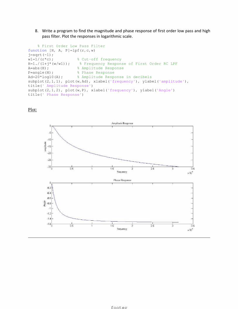
8. Write a program to find the magnitude and phase response of first order low pass and
high pass filter. Plot the responses in logarithmic scale.
9. Write a program to find the response of a low pass filter and high pass filter, when a
speech signal is passed through these filters.
10. Write a program to find the autocorrelation and cross correlation of sequences.
11. Generate a uniformly distributed length 1000 random sequence in the range (0,1). Plot
the histogram and the probability function for the sequence. Compute the mean and
variance of the random signal.
12. Generate a Gaussian distributed length 1000 random sequence . Compute the mean
and variance of the random signal by a suitable method.
13. Write a program to generate a random sinusoidal signal and plot four possible
realizations of the random signal.
14. Generate a discrete time sequence of N=1000 i.i.d uniformly distributed random
numbers in the interval (-0.5,-0.5) and compute the autocorrelation of the sequence.
15. Obtain and plot the power spectrum of the output process when a white random
process is passed through a filter with specific impulse response .
footer

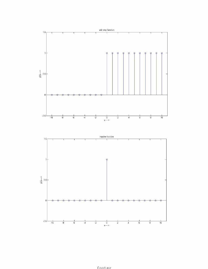
1. Write a program to generate the discrete sequences (i) unit step (ii) unit impulse (iii) ramp (iv)
periodic sinusoidal sequences. Plot all the sequences.
% Unit Step Function function y=unit_step(n) l=length(n); for i=1:l if (n(i)<0) y(i)=0; else y(i)=1; end end figure, stem(n,y), axis([n(1)-1 n(l)+1 -0.5 1.5]) xlabel( 'n----->' ), ylabel( 'y(n)----->' ) title( 'unit step function' )
%Unit Impulse Function function y=impuls(n) l=length(n); for i=1:l if (n(i)~=0) y(i)=0; else y(i)=1; end end figure, stem(n,y), axis([n(1)-1 n(l)+1 -0.5 1.5]) xlabel( 'n----->' ), ylabel( 'y(n)----->' ) title( 'impulse function' )
%Ramp Function function y=ramp(n) l=length(n); for i=1:l y(i)=n(i); end figure, stem(n,y), xlabel( 'n----->' ), ylabel( 'y(n)----->' ) title( 'Ramp function' )
%Sin Function function y=sine(n) l=length(n); y=sin(n); figure, stem(n,y), axis([n(1)-1 n(l)+1 -1.5 1.5]) xlabel( 'n----->' ), ylabel( 'y(n)----->' ),title( 'sin function' ) Plots:
footer
footer

2. Find the Fourier transform of a square pulse .Plot its amplitude and phase spectrum.
footer
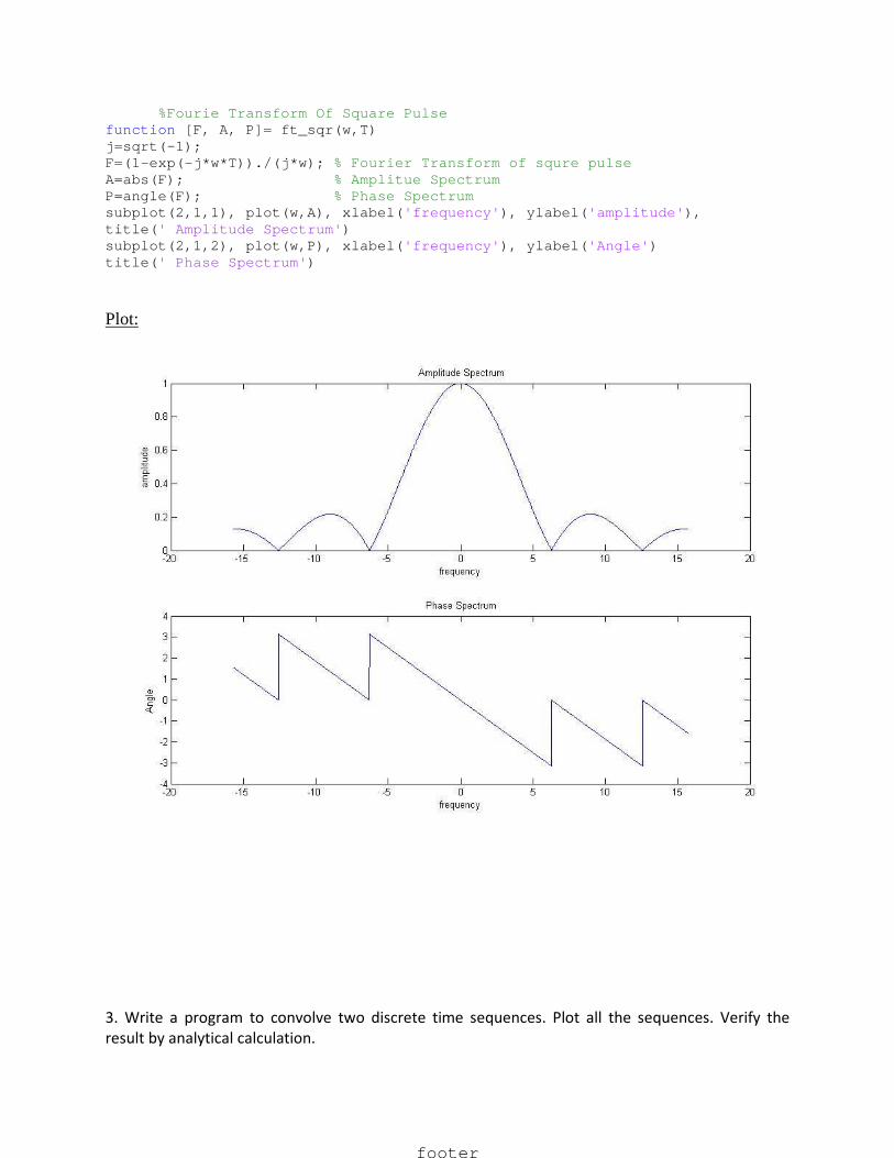
%Fourie Transform Of Square Pulse function [F, A, P]= ft_sqr(w,T) j=sqrt(-1); F=(1-exp(-j*w*T))./(j*w); % Fourier Transform of squre pulse A=abs(F); % Amplitue Spectrum P=angle(F); % Phase Spectrum subplot(2,1,1), plot(w,A), xlabel( 'frequency' ), ylabel( 'amplitude' ), title( ' Amplitude Spectrum' ) subplot(2,1,2), plot(w,P), xlabel( 'frequency' ), ylabel( 'Angle' ) title( ' Phase Spectrum' )
Plot:
3. Write a program to convolve two discrete time sequences. Plot all the sequences. Verify the
result by analytical calculation.
footer

%Discrete Convolution function f=cnv(a,b) la=length(a); lb=length(b); n=la+lb-1; b=[b zeros(1,la-1)]; a=[a zeros(1,lb-1)]; for i=1:n f(i)=0; for j=1:i f(i)=f(i)+a(j)*b(i-j+1); end end
footer

4. Write a program to find the trigonometric Fourier series coefficients of a rectangular periodic
signal. Reconstruct the signal by combining the Fourier series coefficients with appropriate
weightings.
% Trignometric Fourier Series function f=four_rect(n,t,T,k) wo=(2*pi/T); for i=1:n a(i)=2*sin(2*pi*i*t/T)/(pi*i); end disp( 'Trignometric coefficients:' ) ao=(2*t/T); %signal reconstruction for j=1:length(k) f(j)=ao; for i=1:n f(j)=f(j)+a(i)*cos(i*wo*k(j)); end end plot(k,f)
Plot:
footer

5. Write a program to find the trigonometric and exponential fourier series coefficients of a periodic
rectangular signal. Plot the discrete spectrum of the signal.
% Exponential Fourier Series function y=exp_four_rect(n,t,T,k,w) wo=2*pi/T; for i=1:n f(i)=(2*t*sinc(2*i*t/T)/T); f1(i)=(2*t*sinc(2*(-i)*t/T)); end fo=(2*t/T); j=sqrt(-1); for l=1:length(k) y(l)=fo; for m=1:n y(l)=y(l)+f(m)*exp(-j*m*wo*k(l)); end for m=n+1:2*n y(l)=y(l)+f1(m-n)*exp(j*(m-n)*wo*k(l)); end end F=fft(y); subplot(2,1,1), plot(k,y), title( 'Reconstructed Signal' ) subplot(2,1,2), stem(abs(F)), title( 'Discrete Spectrum' )
Plot:
footer

6. Generate a discrete time sequence by sampling a continuous time signal. Show that with
sampling rates less than Nyquist rate, aliasing occurs while reconstructing the signal.
%Sampling Function function y=sa(f,fs) T=1/f; Ts=1/fs; t=0:(pi/1000):2*pi; d=pi/1000; x=sin(2*pi*f*t); l=length(t); j=1; for i=1:l if (t(i)/Ts==round(t(i)/Ts)) y(j)=x(i); j=j+1; elseif (abs(t(i)-j*Ts)<d) if ((abs(t(i)-j*Ts))<=abs(t(i+1)-j*Ts)) y(j)=x(i); j=j+1; elseif ((abs(t(i)-j*Ts))>abs(t(i+1)-j*Ts)) y(j)=x(i+1); j=j+1; end end end subplot(3,1,1), plot(t,x), xlabel( 'time' ), ylabel( 'amplitude' ) title( 'continous signal' ) subplot(3,1,2), stem(y), xlabel( 'time' ), ylabel( 'amplitude' ) title( 'discrete signal' ) subplot(3,1,3), plot(y), xlabel( 'time' ), ylabel( 'amplitude' ) title( 'reconstructed signal' )
footer

Plot:
Under Sampling
Greater Than Nyquist Rate
footer

7. The signal x (t) is defined as below. The signal is sampled at a sampling rate of 1000 samples per second. Find the power content and power spectral density for this signal.
cos(2π × 47t )+ cos(2π × 219t), 0 ≤ t ≤ 10
x(t ) = 0, otherwise
function p=psd() t=0:(1/1000):10; x=cos(2*pi*47*t)+cos(2*pi*219*t); l=length(x); p=(norm(x)^2)/l; ps=spectrum(x,1024); specplot(ps,1000)
footer
8. Write a program to find the magnitude and phase response of first order low pass and high
pass filter. Plot the responses in logarithmic scale.
% First Order Low Pass Filter function [H, A, P]=lpf(r,c,w) j=sqrt(-1); w1=1/(r*c); % Cut-off frequency H=1./(1+j*(w/w1)); % Frequency Response of First Order RC LPF A=abs(H); % Amplitude Response P=angle(H); % Phase Response Ad=20*log10(A); % Amplitude Response in decibels subplot(2,1,1), plot(w,Ad), xlabel( 'frequency' ), ylabel( 'amplitude' ), title( ' Amplitude Response' ) subplot(2,1,2), plot(w,P), xlabel( 'frequency' ), ylabel( 'Angle' ) title( ' Phase Response' )
Plot:
footer

% First Order High Pass Filter function [H, A, P]=hpf(r,c,w) j=sqrt(-1); w1=1/(r*c); % Cut-off frequency H=w./(w-j*w1); % Frequency Response of First Order RC HPF A=abs(H); % Amplitude Response P=angle(H); % Phase Response Ad=20*log10(A); % Amplitude Response in decibels subplot(2,1,1), plot(w,Ad), xlabel( 'frequency' ), ylabel( 'amplitude' ), title( ' Amplitude Response' ) subplot(2,1,2), plot(w,P), xlabel( 'frequency' ), ylabel( 'Angle' ) title( ' Phase Response' )
Plot:
footer
9. Write a program to find the response of a low pass filter and high pass filter, when a
speech signal is passed through these filters. function [Y1 Y2]=speech_response(x,w,w1) j=sqrt(-1); H1=1./(1+j*(w/w1)); %Impulse response of lPF H2=w./(w-j*w1); %Impulse response of HPF X=fft(x); Y1=X.*H1; Y2=X.*H2; subplot(2,1,1), plot(Y1,w) subplot(2,1,2), plot(Y2,w)
footer

10. Write a program to find the autocorrelation and cross correlation of sequences.
% Auto Correlation
function c=cor(a) l=length(a); n=2*l-1; a=[a zeros(1,l-1)]; d(1:l)=a(l:-1:1); % sequence time reverse d=[d zeros(1,l-1)]; for i=1:n c(i)=0; for j=1:i c(i)=c(i)+a(j)*d(i-j+1); % performing convolution to given sequence % and time revers ed gives correlation end end
%Cross correlation
function c=xcor(a,b) la=length(a); lb=length(b); n=la+lb-1; a=[a zeros(1,lb-1)]; d(1:lb)=b(lb:-1:1); % sequence time reverse d=[d zeros(1,la-1)]; for i=1:n c(i)=0; for j=1:i c(i)=c(i)+a(j)*d(i-j+1); % performing convolution to given sequence % and time revers ed gives cross correlation end end
footer
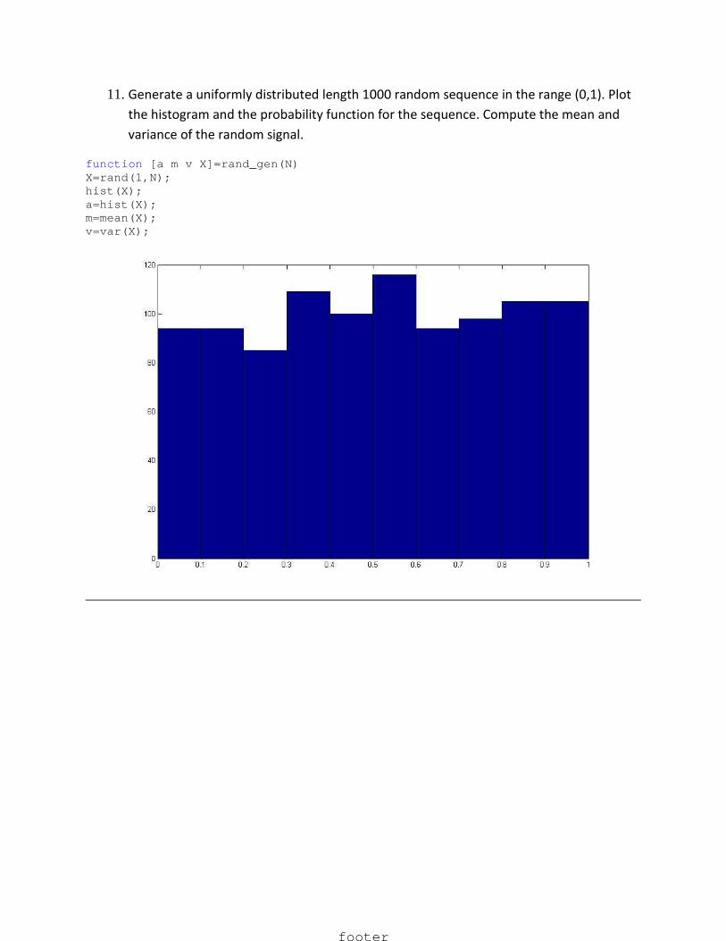
11. Generate a uniformly distributed length 1000 random sequence in the range (0,1). Plot
the histogram and the probability function for the sequence. Compute the mean and
variance of the random signal.
function [a m v X]=rand_gen(N) X=rand(1,N); hist(X); a=hist(X); m=mean(X); v=var(X);
footer

12. Generate a Gaussian distributed length 1000 random sequence . Compute the mean
and variance of the random signal by a suitable method.
function [x m v]=rand_gauss(n) x=rand(1,n); m=mean(x); v=var(x);
footer

13. Write a program to generate a random sinusoidal signal and plot four possible
realizations of the random signal.
function [y1 y2 y3 y4]=rand_sin(n) x1=rand(1,n); x2=rand(1,n); x3=rand(1,n); x4=rand(1,n); y1=sin(x1); y2=sin(x2); y3=sin(x3); y4=sin(x4); subplot(2,2,1), plot(x1,y1) subplot(2,2,2), plot(x2,y2) subplot(2,2,3), plot(x3,y3) subplot(2,2,4), plot(x4,y4)
footer

14. Generate a discrete time sequence of N=1000 i.i.d uniformly distributed random
numbers in the interval (-0.5,-0.5) and compute the autocorrelation of the sequence.
function [x rx]=randseq(n) x=rand(1,n)-0.5; rx=cor(x);
footer

15. Obtain and plot the power spectrum of the output process when a white random
process is passed through a filter with specific impulse response .
function sy=white_rand(w,H) sy=abs(H).^2; plot(w,sy)
footer
Top Related