


Languages
Pages
Legal

Parametric Simulationusing OpenModelica
Enterprise ArchitectUser Guide Series
Author: Sparx Systems
Date: 15/07/2016
Version: 1.0
CREATED WITH
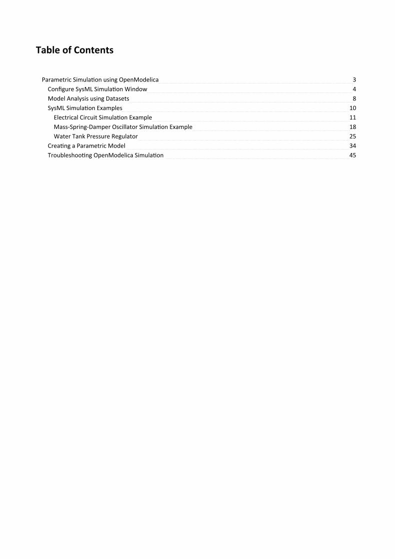
Table of Contents
Parametric Simulation using OpenModelica 3Configure SysML Simulation Window 4Model Analysis using Datasets 8SysML Simulation Examples 10
Electrical Circuit Simulation Example 11Mass-Spring-Damper Oscillator Simulation Example 18Water Tank Pressure Regulator 25
Creating a Parametric Model 34Troubleshooting OpenModelica Simulation 45
User Guide - Parametric Simulation using OpenModelica 15 July, 2016
Parametric Simulation using OpenModelica
Enterprise Architect provides integration with OpenModelica to support rapid and robust evaluation of how a SysMLmodel will behave in different circumstances.
This document describes the process of defining a Parametric model, annotating the model with additional information todrive a simulation and running a simulation to generate a graph.
Introduction to SysML Parametric Models
SysML Parametric models support the engineering analysis of critical system parameters, including the evaluation of keymetrics such as performance, reliability and other physical characteristics. These models combine requirements modelswith system design models by capturing executable constraints based on complex mathematical relationships. Parametricdiagrams are specialized Internal Block diagrams that help you, the modeler, to combine behavior and structure modelswith engineering analysis models such as performance, reliability, and mass property models.
For further information on the concepts of SysML Parametric models, refer to the official OMG SysML website and itslinked sources.
SysMLSimConfiguration Artifact
Enterprise Architect helps you to extend the usefulness of your SysML parametric models by annotating them with extrainformation that allows the model to be simulated. The resulting model is then generated as a Modelica model and can besolved using OpenModelica.
The simulation properties for your model are stored against a Simulation Artifact. This preserves your original model andsupports multiple simulations being configured against a single SysML model. The Simulation Artifact can be found onthe 'Artifacts' Toolbox page.
User Interface Reference
The user interface for the SysML simulation is described in the SysML Simulation Configuration topic.
OpenModelica Example
To aid your understanding of how to create and simulate a SysML parametric model, three examples have been providedto cover three different domains. These examples and what you are able to learn from them are described in the SysMLSimulation Examples topic.
(c) Sparx Systems 2015 - 2016 Page 3 of 46 Created with Enterprise Architect

User Guide - Parametric Simulation using OpenModelica 15 July, 2016
Configure SysML Simulation Window
The Configure SysML Simulation window is the interface through which you can provide run-time parameters forexecuting the simulation of a SysML model. The simulation is based on a simulation configuration defined in aSysMLSimConfiguration Artifact element.
Access
Ribbon Simulate > SysMLSim > Manage > SysMLSim Configuration Manager
Other Double click on an Artifact with the SysMLSimConfiguration stereotype.
Toolbar Options
Option Description
Click on the drop-down arrow and select from these options:
Select Artifact - Select and load an existing configuration from an Artifact with·the SysMLSimConfiguration stereotype (if one has not already been selected)
Create Artifact - Create a new SysMLSimConfiguration or select and load an·existing configuration artifact
Select Package - Select a Package to scan for SysML elements to configure for·simulation
Reload - Reload the Configuration Manager with changes to the current·Package
Configure Modelica Solver - Display the 'Modelica Solver Path' dialog, in·
(c) Sparx Systems 2015 - 2016 Page 4 of 46 Created with Enterprise Architect

User Guide - Parametric Simulation using OpenModelica 15 July, 2016
which you type or browse for the path to the Modelica solver to use
Click on this button to save the configuration to the current Artifact.
Click on this button to generate, compile and run the current configuration, anddisplay the results.
After simulation, the result file is generated in either plt, mat or csv format. That is,with the filename:
ModelName_res.plt·ModelName_res.mat or·ModelName_res.csv·
Click on this button to specify a directory into which Enterprise Architect will copythe result file.
Click on this button to select from these options:
Generate Modelica Code - Generate the code without compiling or running it·Open Modelica Simulation Directory - Open the directory into which Modelica·code will be generated
Edit Modelica Templates - Customize the code generated for Modelica, using·the Code Template Editor
Simulation Artifact and Model Selection
Field Meaning
ArtifactClick on the icon and either browse for and select an existingSysMLSimConfiguration Artifact, or create a new Artifact.
Package If you have specified an existing SysMLSimConfiguration Artifact, this fielddefaults to the Package containing the SysML model associated with that Artifact.
Otherwise, click on the icon and browse for and select the Package containingthe SysML model to configure for simulation. You must specify the Artifact beforeselecting the Package.
(c) Sparx Systems 2015 - 2016 Page 5 of 46 Created with Enterprise Architect

User Guide - Parametric Simulation using OpenModelica 15 July, 2016
Package Elements
This table discusses the element types from the SysML model that will be listed under the 'Name' column in theConfigure SysML Simulation window, to be processed in the simulation.
Element Type Behavior
ValueType ValueType elements either generalize from a primitive type or are substituted bySysMLSimReal for simulation.
Block Block elements mapped to SysMLSimClass or SysMLSimModel elements supportthe creation of data set(s). In the case of multiple data sets, a SysMLSimClass mustdefine one of them as the default; a SysMLSimModel is a possible top levelelement for a simulation, and a data set is chosen on simulation.
Properties Properties within a block can be configured to be either SimConstants orSimVariables. For a SimVariable, you configure these attributes:
isContinuous - determines whether the property value varies continuously·('True', the default) or discretely ('False')
isConserved - determines whether values of the property are conserved ('True')·or not ('False', the default); when modeling for physical interaction, theinteractions include exchanges of conserved physical substances such aselectrical current, force or fluid flow
changeCycle - specifies the time interval at which a discrete property value·changes; the default value is '0' - changeCycle can be set to a value other than 0 only when isContinuous ='False' - The value of changeCycle must be positive or equal to 0
Port No configuration required.
SimFunction Functions are created as operations in Blocks or Constraint Blocks, stereotyped as'SimFunction'.
No configuration is required in the Configure SysML Simulation window.
Generalization No configuration required.
Binding Connector Binds a property to a parameter of a constraint property.
No configuration required.
Connector Connects two Ports.
No configuration required in the Configure SysML Simulation window. However,you might have to configure the properties of the Port's type by determiningwhether the attribute isConserved should be set as 'False' (for potential properties,so that equality coupling is established) or 'True' (for flow/conserved properties, sothat sum-to-zero coupling is established).
Constraint Block No configuration required.
Simulation Tab
(c) Sparx Systems 2015 - 2016 Page 6 of 46 Created with Enterprise Architect
User Guide - Parametric Simulation using OpenModelica 15 July, 2016
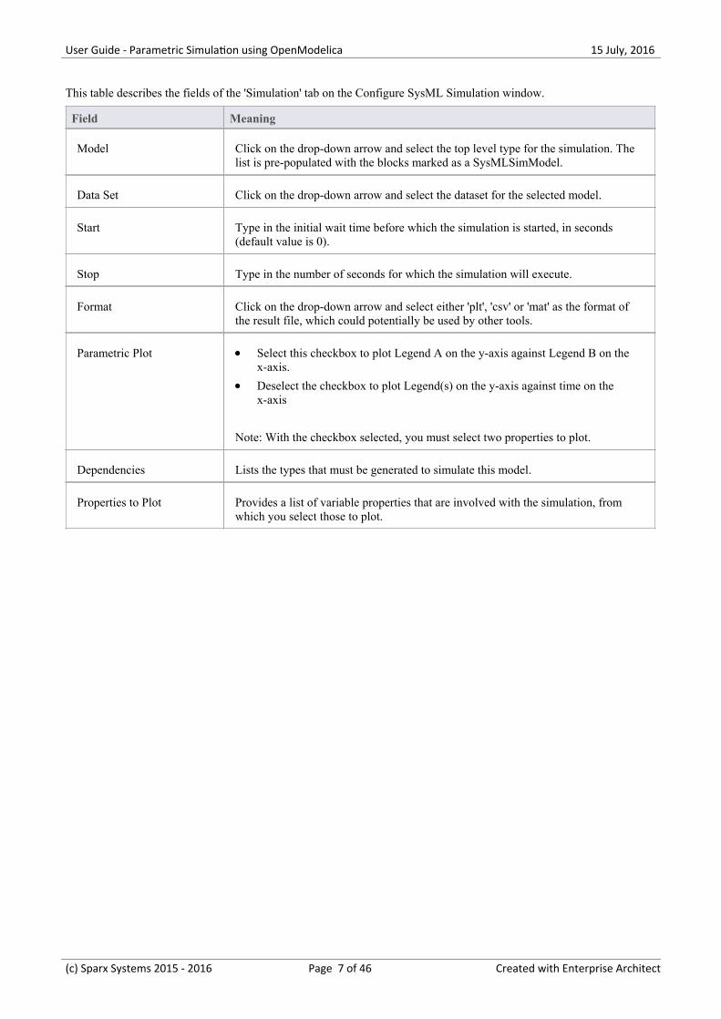
This table describes the fields of the 'Simulation' tab on the Configure SysML Simulation window.
Field Meaning
Model Click on the drop-down arrow and select the top level type for the simulation. Thelist is pre-populated with the blocks marked as a SysMLSimModel.
Data Set Click on the drop-down arrow and select the dataset for the selected model.
Start Type in the initial wait time before which the simulation is started, in seconds(default value is 0).
Stop Type in the number of seconds for which the simulation will execute.
Format Click on the drop-down arrow and select either 'plt', 'csv' or 'mat' as the format ofthe result file, which could potentially be used by other tools.
Parametric Plot Select this checkbox to plot Legend A on the y-axis against Legend B on the·x-axis.
Deselect the checkbox to plot Legend(s) on the y-axis against time on the·x-axis
Note: With the checkbox selected, you must select two properties to plot.
Dependencies Lists the types that must be generated to simulate this model.
Properties to Plot Provides a list of variable properties that are involved with the simulation, fromwhich you select those to plot.
(c) Sparx Systems 2015 - 2016 Page 7 of 46 Created with Enterprise Architect

User Guide - Parametric Simulation using OpenModelica 15 July, 2016
Model Analysis using Datasets
Every SysML block used in a Parametric model can have multiple datasets defined against them. This allows forrepeatable simulation variations using the same SysML model. When running a simulation, a user is able to select fromthe datasets specified against the model before starting.
Dataset Management
Create New Datasets can be created by right clicking on a block selecting 'CreateSimulation Dataset'.
Duplicate To duplicate an existing dataset as a base for creating a new dataset, right click onthe dataset and select 'Duplicate'.
Delete To remove a dataset that is no longer required, right click on the dataset and select'Delete Dataset'.
Set Default The default dataset used by a SysMLSimClass when used as a property type orinherited can be set by right clicking on the dataset and selecting 'Set as Default'.The properties used by a model will use this default configuration unless the modeloverrides them explicitly.
Configure Simulation Data
Attribute The Attribute column provides a tree view of all the properties in the Block beingedited.
(c) Sparx Systems 2015 - 2016 Page 8 of 46 Created with Enterprise Architect

User Guide - Parametric Simulation using OpenModelica 15 July, 2016
Stereotype The stereotype column specifies for each property if it has been configured to be aconstant for the duration of the simulation or variable so that the value is expectedto change over time.
Type The Type column describes the type used for simulation of this property. It can beeither a primitive type (eg. Real) or a reference to a Block contained in the model.Properties referencing blocks will show the child properties specified by thereferenced block below them.
Default Value The default value column shows the value that will be used in the simulation if nooverride is provided. This can come from the Initial Value field in the SysMLmodel or from the default dataset of the parent type.
Value The value column allows the user to override the default value for each primitivevalue.
Export / Import The export and import buttons allow the user to modify the values in the currentdataset using an external application such as a spreadsheet before re-importingthem.
(c) Sparx Systems 2015 - 2016 Page 9 of 46 Created with Enterprise Architect
User Guide - Parametric Simulation using OpenModelica 15 July, 2016
SysML Simulation Examples
This section provides three worked examples of how to create a SysML model for a domain, simulate it and evaluate theresults of the simulation. These examples apply the information discussed in the earlier topics.
Electrical Circuit Simulation Example
The first example, is for simulation of an electrical circuit. The example starts with an electrical circuit diagram, convertsit to a parametric model. The model is then simulated and the voltage at the source and target wires of a resistor areevaluated and compared to the expected values.
Electrical Circuit Simulation Example
Mass-Spring-Damper Oscillator Simulation Example
The second example uses a simple physical model to demonstrate the oscillation behavior of a string under tension.
Mass-Spring-Damper Oscillator Simulation Example
Water Tank Pressure Regulator
The final example shows the water levels of two water tanks where the water is being distributed between them. We firstsimulate a well balanced system, then we simulate a system where the water will overflow from the second tank.
Water Tank Pressure Regulator
(c) Sparx Systems 2015 - 2016 Page 10 of 46 Created with Enterprise Architect

User Guide - Parametric Simulation using OpenModelica 15 July, 2016
Electrical Circuit Simulation Example
In this section, we will walk through the creation of a SysML parametric model for a simple electrical circuit, and thenuse a parametric simulation to predict and chart the behavior of that circuit.
Circuit Diagram
The electrical circuit we are going to model is shown below using a standard electrical circuit notation.
The circuit includes an AC power source, a ground and a resistor. Each of these being connected via wires.
Create SysML Model
The following table shows how we can build up a complete SysML model to represent the circuit. Starting at the lowestlevel types and building up the model one step at a time.
Types Define Value Types for each of Voltage, Current and Resistance. Unit and quantitykind are not important for the purpose of simulation but would be set if defining acomplete SysML model. These types will be generalized from the primitive type'Real'. In other models, you can choose to map a value type to a correspondingsimulation type separate from the model.
«valueType»Voltage
quantityKind = unit =
«valueType»Current
quantityKind = unit =
«valueType»Resistance
quantityKind = unit =
Additionally, we define a composite type called ChargePort, which includesproperties for both Current and Voltage. This type allows us to represent theelectrical energy at the connectors between components.
(c) Sparx Systems 2015 - 2016 Page 11 of 46 Created with Enterprise Architect
User Guide - Parametric Simulation using OpenModelica 15 July, 2016
«block»ChargePort
flow properties none i : Current none v : Voltage
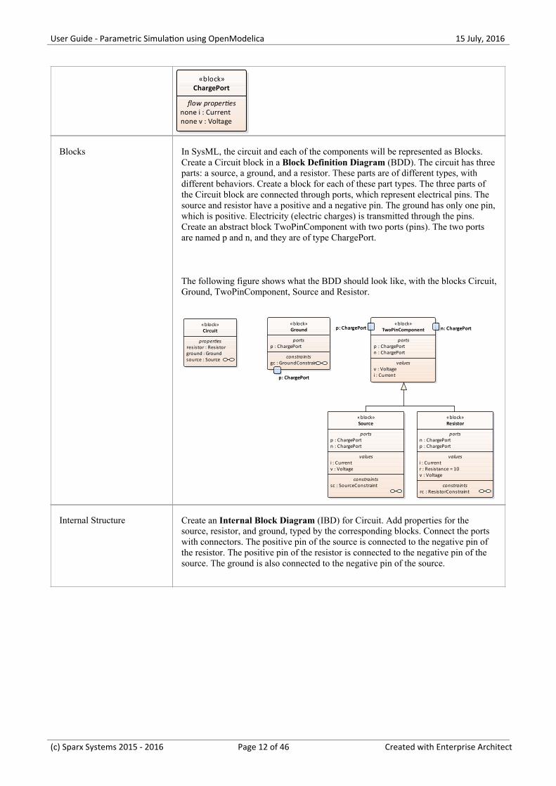
Blocks In SysML, the circuit and each of the components will be represented as Blocks.Create a Circuit block in a Block Definition Diagram (BDD). The circuit has threeparts: a source, a ground, and a resistor. These parts are of different types, withdifferent behaviors. Create a block for each of these part types. The three parts ofthe Circuit block are connected through ports, which represent electrical pins. Thesource and resistor have a positive and a negative pin. The ground has only one pin,which is positive. Electricity (electric charges) is transmitted through the pins.Create an abstract block TwoPinComponent with two ports (pins). The two portsare named p and n, and they are of type ChargePort.
The following figure shows what the BDD should look like, with the blocks Circuit,Ground, TwoPinComponent, Source and Resistor.
«block»Source
ports p : ChargePort n : ChargePort
values i : Current v : Voltage
constraints sc : SourceConstraint
«block»Circuit
properties res istor : Resistor ground : Ground source : Source
p: ChargePort
«block»Ground
ports p : ChargePort
constraints gc : GroundConstraint
p: ChargePort
p: ChargePort n: ChargePort«block»
TwoPinComponent
ports p : ChargePort n : ChargePort
values v : Voltage i : Current
p: ChargePort n: ChargePort
«block»Resistor
ports n : ChargePort p : ChargePort
values i : Current r : Resistance = 10 v : Voltage
constraints rc : ResistorConstraint
Internal Structure Create an Internal Block Diagram (IBD) for Circuit. Add properties for thesource, resistor, and ground, typed by the corresponding blocks. Connect the portswith connectors. The positive pin of the source is connected to the negative pin ofthe resistor. The positive pin of the resistor is connected to the negative pin of thesource. The ground is also connected to the negative pin of the source.
(c) Sparx Systems 2015 - 2016 Page 12 of 46 Created with Enterprise Architect

User Guide - Parametric Simulation using OpenModelica 15 July, 2016
ibd [block] Circuit [Circuit]
n: ChargePort
p: ChargePort
source: Source
n: ChargePort
p: ChargePort n: ChargePort
p: ChargePort
resistor: Resistor
n: ChargePort
p: ChargePort
p: ChargePort
ground: Ground
p: ChargePort
Notice that this follows the same structure as the original circuit diagram, but thesymbols for each component have been replaced with properties typed by theblocks defined above.
Constraints Equations define mathematical relationships between numeric properties. InSysML, equations are represented as constraints in constraint blocks. Parameters ofconstraint blocks correspond to SimVariables and SimConstant of blocks (i, v, r inthis example), as well as to SimVariables present in the type of the ports (pv, pi, nv,ni in this example).
Create an constraint block TwoPinComponentConstraint to define parameters andequations common to sources and resistors. The equations should state that thevoltage of the component is equal to the difference between the voltage at thepositive and negative pin. The current of the component is equal to the currentgoing through the positive pin. The sum of the current going through the two pinsmust add up to zero (one is the negative of the other). The ground constraint statesthat the voltage at the ground pin is zero. The source constraint defines the voltageas a sine wave with the current simulation time as parameter. The following figureshows what these constraints should look like in a BDD.
(c) Sparx Systems 2015 - 2016 Page 13 of 46 Created with Enterprise Architect

User Guide - Parametric Simulation using OpenModelica 15 July, 2016
«constraint»TwoPinComponentConstraint
constraints{pi+ni=0}{i=pi}{v=pv-nv}
parameters i : Real ni : Real nv : Real pi : Real pv : Real v : Real
«constraint»GroundConstraint
constraints{pv=0}
parameters pv : Real
«constraint»ResistorConstraint
constraints{v=r*i}
parameters i : Real ni : Real nv : Real pi : Real pv : Real r : Real v : Real
«constraint»SourceConstraint
constraints{v=sin(time)}
parameters i : Real ni : Real nv : Real pi : Real pv : Real v : Real
Bindings The values of constraint parameters are equated to variable and constant valueswith binding connectors. Create constraint properties on each block (propertiestyped by constraint blocks) and bind the block variables and constants to theconstraint parameters to apply the constraint to the block. block. The followingfigures show the bindings for the ground, the source, and the resistor respectively.
For the ground constraint, bind gc.pv to p.v.
p: ChargePort
par [block] Ground [Ground]
p: ChargePort
v : Voltage
gc : GroundConstraint{pv=0}
pv : Real«equal»
For the source constraint, bind sc.pi to p.i, sc.pv to p.v, sc.v to v, sc.i to i, sc.ni ton.i, and sc.nv to n.v .
(c) Sparx Systems 2015 - 2016 Page 14 of 46 Created with Enterprise Architect
User Guide - Parametric Simulation using OpenModelica 15 July, 2016
p: ChargePort n: ChargePort
par [block] Source [Source]
p: ChargePort n: ChargePort
i: Current v: Voltage
sc : SourceConstraint{v=sin(time)}
i : Real v : Real
ni : Real
nv : Real
pi : Real
pv : Realv : Voltage
i : Current
v : Voltage
i : Current«equal»
«equal»«equal»
«equal»«equal»
«equal»
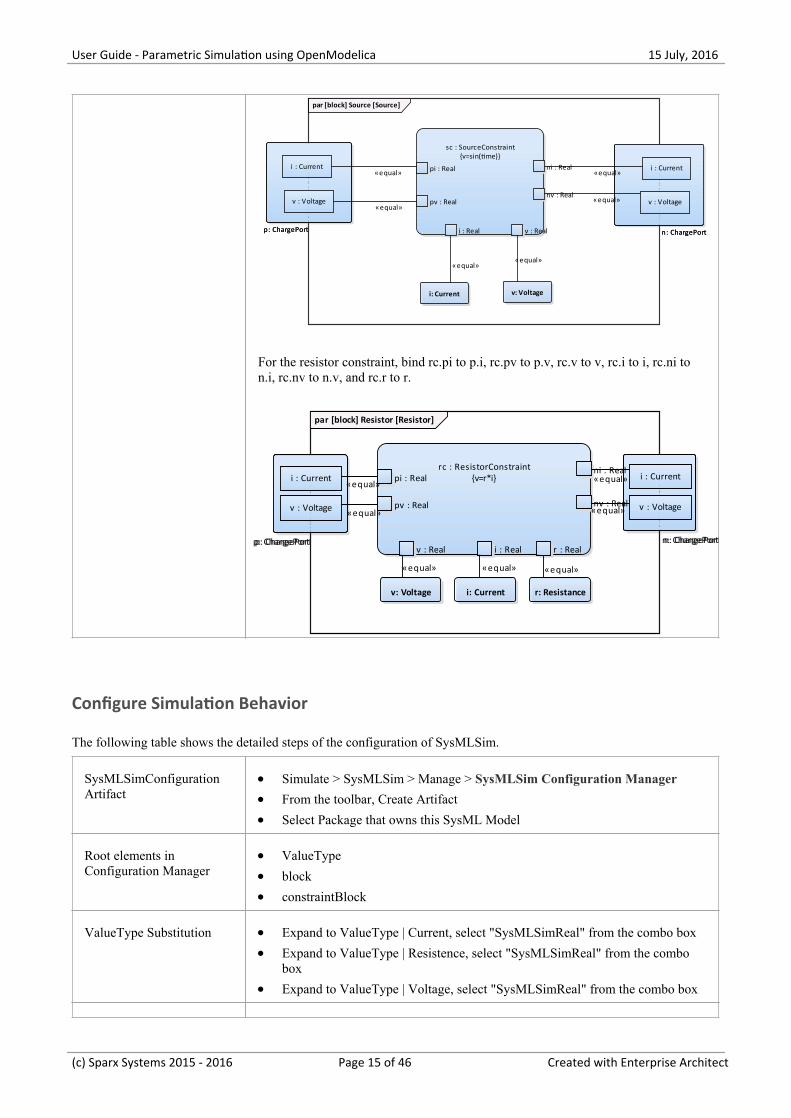
For the resistor constraint, bind rc.pi to p.i, rc.pv to p.v, rc.v to v, rc.i to i, rc.ni ton.i, rc.nv to n.v, and rc.r to r.
n: ChargePortp: ChargePort
par [block] Resistor [Resistor]
n: ChargePortp: ChargePort
r: Resistance
rc : ResistorConstraint{v=r*i}
pv : Real
pi : Real
nv : Real
ni : Real
v : Real i : Real r : Real
v: Voltage i: Current
v : Voltage
i : Current
v : Voltage
i : Current
«equal»
«equal»
«equal» «equal»
«equal» «equal»
«equal»
Configure Simulation Behavior
The following table shows the detailed steps of the configuration of SysMLSim.
SysMLSimConfigurationArtifact
Simulate > SysMLSim > Manage > SysMLSim Configuration Manager·From the toolbar, Create Artifact·Select Package that owns this SysML Model·
Root elements inConfiguration Manager
ValueType·block·constraintBlock·
ValueType Substitution Expand to ValueType | Current, select "SysMLSimReal" from the combo box·Expand to ValueType | Resistence, select "SysMLSimReal" from the combo·box
Expand to ValueType | Voltage, select "SysMLSimReal" from the combo box·
(c) Sparx Systems 2015 - 2016 Page 15 of 46 Created with Enterprise Architect
User Guide - Parametric Simulation using OpenModelica 15 July, 2016
Set property as flow Expand to block | ChargePort | FlowProperty | i : Current, Select·"SimVariable" from the combo box
Click the "..." button to open the "Element Configurations" dialog·Set "isConserved" to "true"·
SysMLSimModel This is the model we want to simulate: Set block "Circuit" to be SysMLSimModel
Run Simulation
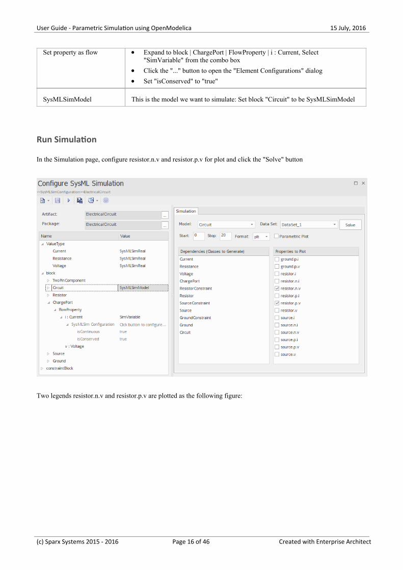
In the Simulation page, configure resistor.n.v and resistor.p.v for plot and click the "Solve" button
Two legends resistor.n.v and resistor.p.v are plotted as the following figure:
(c) Sparx Systems 2015 - 2016 Page 16 of 46 Created with Enterprise Architect

User Guide - Parametric Simulation using OpenModelica 15 July, 2016
(c) Sparx Systems 2015 - 2016 Page 17 of 46 Created with Enterprise Architect

User Guide - Parametric Simulation using OpenModelica 15 July, 2016
Mass-Spring-Damper Oscillator Simulation Example
In this section, we will walk through the creation of a SysML parametric model for a simple Oscillator composed ofmass-spring-damper and then use a parametric simulation to predict and chart the behavior of this mechanical system.Finally, we do some what-if analysis by compare two oscillators provided with different parameter values through datasets.
System being modeled
A mass body hanging on a spring damper. The first state represents the initial point at time = 0 just when the body isreleased. The second state represents the final state when the body is at rest and the spring forces are in equilibrium withthe gravity force.
Create SysML Model
The MassSpringDamperOscillator model in SysML has a main block, the Oscillator. The oscillator has four parts: afixed ceiling, a spring, a damper and a mass body. Create a block for each of these part types. The four parts of theOscillator block are connected through ports, which represent mechanical flanges.
Port Types The block Flange_a and Flange_b used for flanges in the 1D translationalmechanical domain are identical but have slightly different roles, somewhatanalogous to the roles of PositivePin and NegativePin in the electrical domain.Momentum is transmitted through the flanges. So the attribute isConserved of flowproperty Flange.f should be set to true.
(c) Sparx Systems 2015 - 2016 Page 18 of 46 Created with Enterprise Architect
User Guide - Parametric Simulation using OpenModelica 15 July, 2016
«block»Flange_b
«block»Flange
flow properties inout f inout s
«block»Flange_a
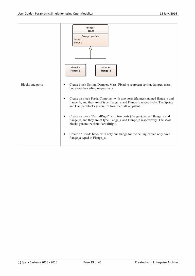
Blocks and ports Create block Spring, Damper, Mass, Fixed to represent spring, damper, mass·body and the ceiling respectively.
Create an block PartialCompliant with two ports (flanges), named flange_a and·flange_b, and they are of type Flange_a and Flange_b respectively. The Springand Damper blocks generalize from PartialCompilant.
Create an block "PartialRigid" with two ports (flanges), named flange_a and·flange_b, and they are of type Flange_a and Flange_b respectively. The Massblocks generalize from PartialRigid.
Create a "Fixed" block with only one flange for the ceiling, which only have·flange_a typed to Flange_a.
(c) Sparx Systems 2015 - 2016 Page 19 of 46 Created with Enterprise Architect

User Guide - Parametric Simulation using OpenModelica 15 July, 2016
«block»Oscillator
properties fixed1 : Fixed damper1 : Damper mass1 : Mass spring1 : Spring
«block»Damper
constraints{v_rel=der(s_rel)}{f = d * v_rel}{lossPower = f * v_rel}
properties d = 25 lossPower v_rel
flange_a:Flange_a
«block»Fixed
constraints{flange_a.s = s0}
properties s0 = 1.0
ports flange_a : Flange_aflange_a:
Flange_a
«block»Mass
constraints{v = der(s)}{a = der(v)}{m*a = flange_a.f + flange_b.f}{flange_a.f = - m * g}
properties a g = 9.81 m = 1 v
flange_b:Flange_b
flange_a:Flange_a
«block»PartialCompliant
constraints{s_rel=flange_b.s - flange_a.s}{flange_b.f = f}{flange_a.f = -f}
properties f s_rel = 0
ports flange_a : Flange_a flange_b : Flange_b
flange_b:Flange_b
flange_a:Flange_a
flange_b:Flange_b
flange_a:Flange_a
«block»PartialRigid
constraints{flange_a.s = s-L/2}{flange_b.s = s + L/2}
properties L = 1 s = -0.5
ports flange_a : Flange_a flange_b : Flange_b
flange_b:Flange_b
flange_a:Flange_a
«block»Spring
constraints{f = c*(s_rel - s_rel0)}
properties c = 10000 s_rel0 = 2
+spring1+damper1+fixed1 +mass1
Internal structure Create an Internal Block Diagram (IBD) for Oscillator. Add properties for thefixed ceiling, spring, damper and mass body, typed by the corresponding blocks.Connect the ports with connectors.
The flang_a of fixed1 connect to flange_b of sprint1·The flange_b of damper1 connect to flange_b of spring1·The flange_a of damper1 connect to flange_a of spring1·The flange_a of spring1 connect to flange_b of mass1·
(c) Sparx Systems 2015 - 2016 Page 20 of 46 Created with Enterprise Architect

User Guide - Parametric Simulation using OpenModelica 15 July, 2016
ibd [block] Oscillator [Oscillator]
flange_a: Flange_a
fixed1: Fixed
flange_a: Flange_a
flange_a: Flange_a
flange_b: Flange_b
spring1: Spring
flange_a: Flange_a
flange_b: Flange_b
flange_a: Flange_a
flange_b: Flange_b
damper1: Damper
flange_a: Flange_a
flange_b: Flange_b
flange_b: Flange_b
mass1: Mass
flange_b: Flange_b
Constraints For simplicity, we defined the constraints directly in the block elements; optionally,you can define constraint blocks and use constraint properties in the blocks andbind their parameters to block's properties.
Two Oscillator Compare Plan
After we had a Oscillator, we want to do some what-if analysis. For example:
What's the difference between two oscillators whose dampers are different?·What if there is no damper?·What's the difference between two oscillators whose springs are different?·What's the difference between two oscillators whose mass are different?·
Here are the steps of creating a compare model:
Craete a block named "OscillatorCompareModel"·Create two properties for "OscillatorCompareModel", give them name oscillator1 and oscillator2, type them with·Block Oscillator
«block»OscillatorCompareModel
properties oscillator1 : Oscillator oscillator2 : Oscillator
oscillator2: Oscillatoroscillator1: Oscillator
Setup DataSet and Run Simulation
Create a SysMLSim Configuration artifact and setup to this package. Then create the following data sets:
Damper: small VS big·
(c) Sparx Systems 2015 - 2016 Page 21 of 46 Created with Enterprise Architect
User Guide - Parametric Simulation using OpenModelica 15 July, 2016
provide "oscillator1.damper1.d" with smaller value 10 and "oscillator1.damper2.d" with bigger value 20
Damper: no vs yes· provide "oscillator1.damper1.d" with value 0; ("oscillator2.damper2.d" will use the default value 25)
Spring: small VS big· provide "oscillator1.spring1.c" with smaller value 6000 and "oscillator1.spring1.c" with bigger value 12000
Mass: light VS heavy· provide "oscillator1.mass1.m" with smaller value 0.5 and "oscillator1.mass1.m" with bigger value 2
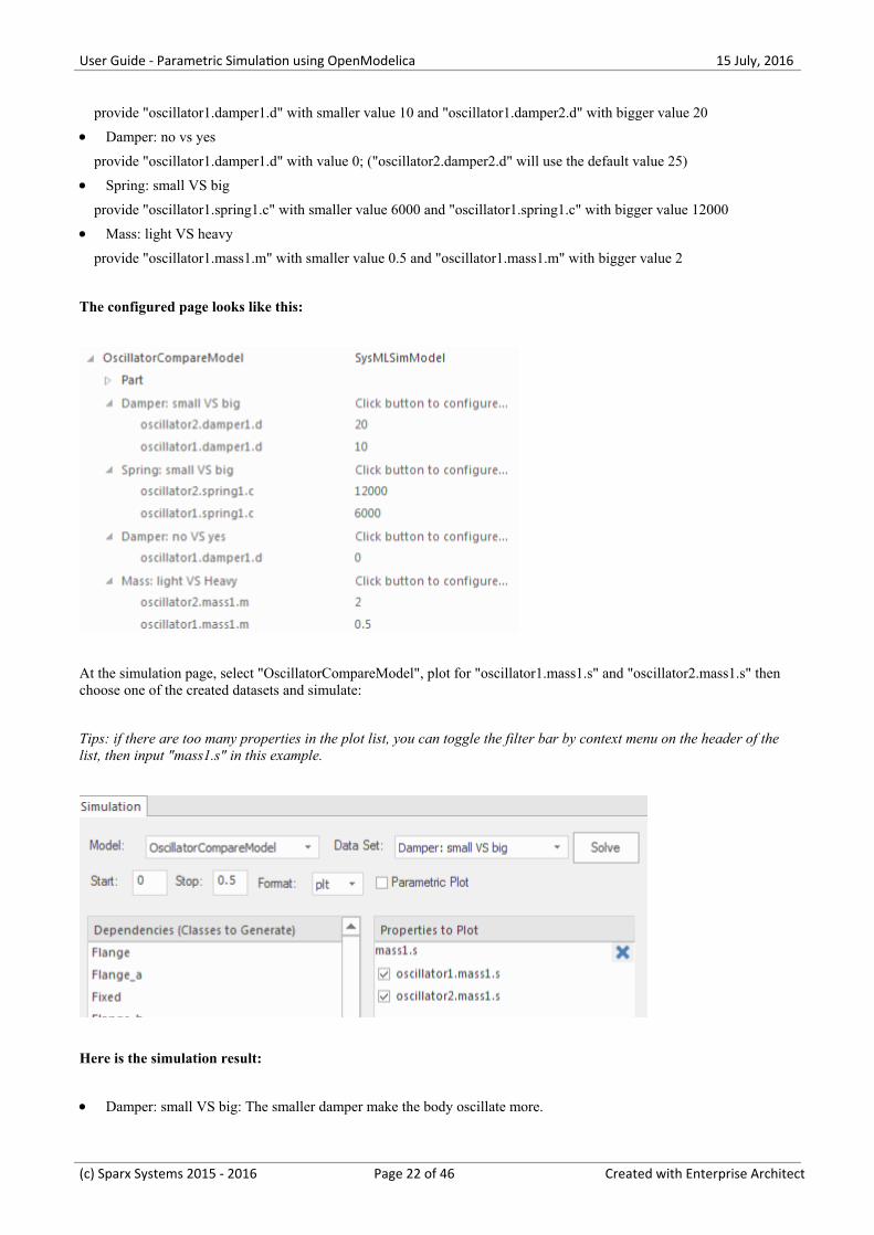
The configured page looks like this:
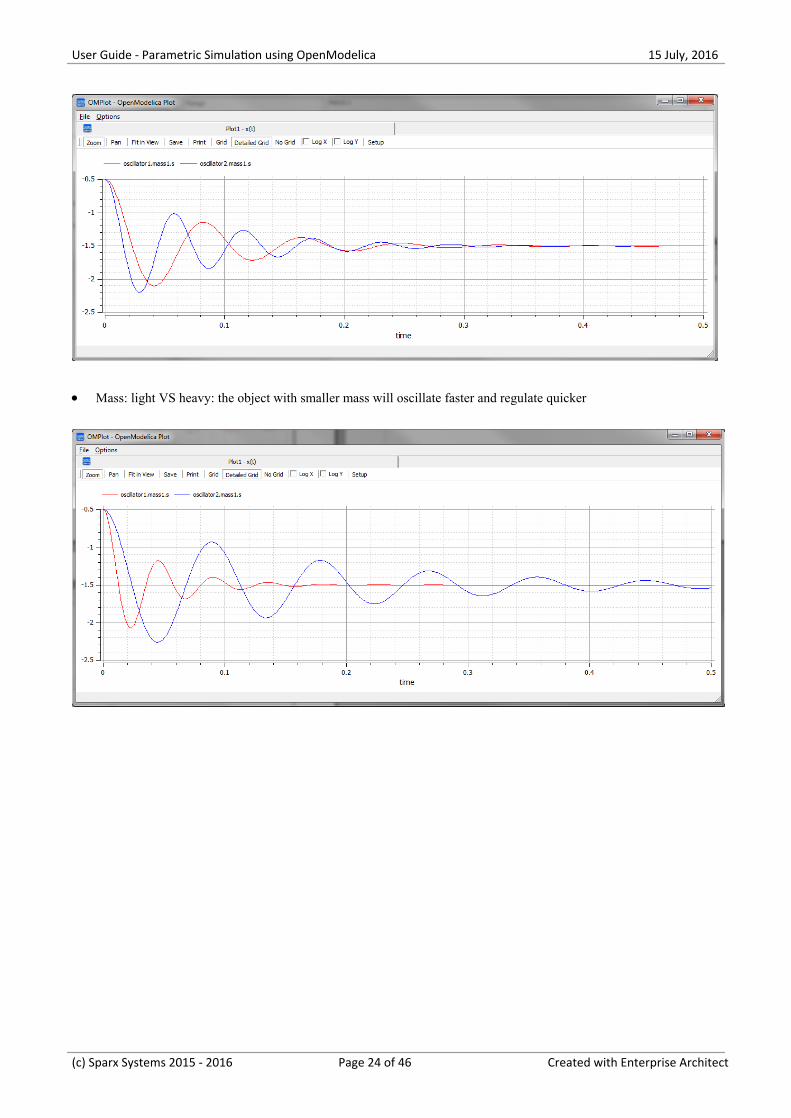
At the simulation page, select "OscillatorCompareModel", plot for "oscillator1.mass1.s" and "oscillator2.mass1.s" thenchoose one of the created datasets and simulate:
Tips: if there are too many properties in the plot list, you can toggle the filter bar by context menu on the header of thelist, then input "mass1.s" in this example.
Here is the simulation result:
Damper: small VS big: The smaller damper make the body oscillate more.·
(c) Sparx Systems 2015 - 2016 Page 22 of 46 Created with Enterprise Architect

User Guide - Parametric Simulation using OpenModelica 15 July, 2016
Damper: no vs yes : the oscillator never stops without a damper·
Spring: small VS big: the spring with smaller "c" will oscillate slower·
(c) Sparx Systems 2015 - 2016 Page 23 of 46 Created with Enterprise Architect
User Guide - Parametric Simulation using OpenModelica 15 July, 2016
Mass: light VS heavy: the object with smaller mass will oscillate faster and regulate quicker·
(c) Sparx Systems 2015 - 2016 Page 24 of 46 Created with Enterprise Architect

User Guide - Parametric Simulation using OpenModelica 15 July, 2016
Water Tank Pressure Regulator
In this section, we will walk through the creation of a SysML parametric model for a Water Tank Pressure Regulatorcomposed of two connected tanks, a source of water and two controllers, each of which monitor the water level andcontrol the valve to regulate the system.
We will get the model explained, create the SysML model and setup the SysMLSim Configurations. Then run thesimulation with OpenModelica.
System being modeled
The following figure represents two tanks connected together, and a source water will fills the first tank. Each tank has acontinuous proportional–integral (PI) controller connected to it, which regulates the level of water contained in the tanksto a reference level. While the source fills the first tank with water the PI continuous controller regulates the outflowfrom the tank depending on its actual level. Water from the first tank flows into the second tank, which the PI continuouscontroller also tries to regulate. This is a natural and non domain specific physical problem.
Create SysML Model
Port Types The tank has four ports, they are typed to the following three blocks:
ReadSignal: Reading fluid level. It has a property val with unit "m"·ActSignal: Signal to actuator for setting valve position·LiquidFlow: Liquid flow at inlets or outlets. It has a property lflow with unit·"m3/s"
(c) Sparx Systems 2015 - 2016 Page 25 of 46 Created with Enterprise Architect
User Guide - Parametric Simulation using OpenModelica 15 July, 2016
«block»ActSignal
flow properties none act : Real
«block»LiquidFlow
flow properties none lflow : Real
«block»ReadSignal
flow properties none val : Real
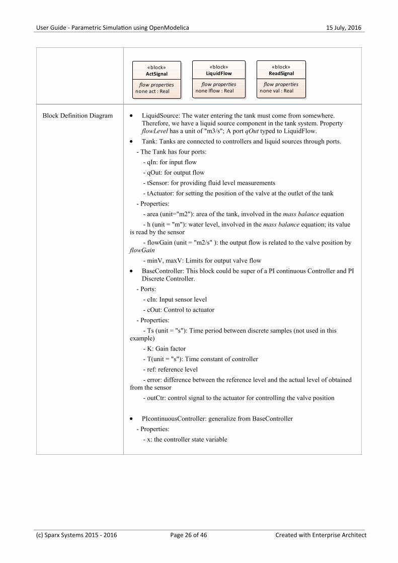
Block Definition Diagram LiquidSource: The water entering the tank must come from somewhere.·Therefore, we have a liquid source component in the tank system. PropertyflowLevel has a unit of "m3/s"; A port qOut typed to LiquidFlow.
Tank: Tanks are connected to controllers and liquid sources through ports.· - The Tank has four ports:
- qIn: for input flow
- qOut: for output flow
- tSensor: for providing fluid level measurements
- tActuator: for setting the position of the valve at the outlet of the tank
- Properties:
- area (unit="m2"): area of the tank, involved in the mass balance equation
- h (unit = "m"): water level, involved in the mass balance equation; its valueis read by the sensor
- flowGain (unit = "m2/s" ): the output flow is related to the valve position byflowGain
- minV, maxV: Limits for output valve flow
BaseController: This block could be super of a PI continuous Controller and PI·Discrete Controller.
- Ports:
- cIn: Input sensor level
- cOut: Control to actuator
- Properties:
- Ts (unit = "s"): Time period between discrete samples (not used in thisexample)
- K: Gain factor
- T(unit = "s"): Time constant of controller
- ref: reference level
- error: difference between the reference level and the actual level of obtainedfrom the sensor
- outCtr: control signal to the actuator for controlling the valve position
PIcontinuousController: generalize from BaseController· - Properties:
- x: the controller state variable
(c) Sparx Systems 2015 - 2016 Page 26 of 46 Created with Enterprise Architect

User Guide - Parametric Simulation using OpenModelica 15 July, 2016
cOut: ActSignal
cIn: ReadSignal
«block»BaseController
properties error : Real K : Real outCtr : Real ref : Real T : Real Ts : Real
ports cIn : ReadSignal cOut : ActSignal
constraints e5 : CoutAct e6 : ErrorValue
cOut: ActSignal
cIn: ReadSignal
qOut: LiquidFlow
«block»LiquidSource
properties flowLevel : Real
ports qOut : LiquidFlow
constraints e4 : OutFlowqOut: LiquidFlow
«block»PIcontinuousController
properties error : Real K : Real outCtr : Real T : Real x : Real
constraints e7 : StateVariable e8 : OutControl
tSensor: ReadSignal
tActuator: ActSignal
qOut: LiquidFlow
qIn: LiquidFlow
«block»Tank
properties flowGain : Real area : Real h : Real maxV : Real = 10 minV : Real = 0
ports qIn : LiquidFlow qOut : LiquidFlow tActuator : ActSignal tSensor : ReadSignal
constraints e1 : Mass_Balance e2 : SensorValue e3 : Q_OutFlow
tSensor: ReadSignal
tActuator: ActSignal
qOut: LiquidFlow
qIn: LiquidFlow
Constraint Blocks The flow increases sharply at time = 150 to factor of three of the previous flowlevel, which creates an interesting control problem that the controller of the tankhas to handle.
qOut: LiquidFlow
par [block] LiquidSource [LiquidSource]
qOut: LiquidFlow
flowLevel: Real
e4 : OutFlow{a = if time > 150 then 3*b else b}
ablflow : Real
«equal» «equal»
The central equation regulating the behavior of the tank is the mass balanceequation.
The output flow is related to the valve position by a flowGain parameter.
The sensor simply read the level of the tank.
qIn: LiquidFlow
qOut: LiquidFlow
tSensor: ReadSignal
tActuator: ActSignal
par [block] Tank [Tank]
qIn: LiquidFlow
qOut: LiquidFlow
tSensor: ReadSignal
tActuator: ActSignal
area: Real
flowGain: Real minV: Real
h: Real
e1 : Mass_Balance{der(h) = (x - y) / a}
e2 : SensorValue{a=b}
e3 : Q_OutFlow{a=LimitValue(min, max, -b*c)}
h
y
a
ab
a
cb max min
x
maxV: Real
lflow : Real
lflow : Real
val : Real
act : Real
«equal»
«equal»
«equal»
«equal» «equal»
«equal»
«equal»
«equal»
«equal»
«equal»
«equal»
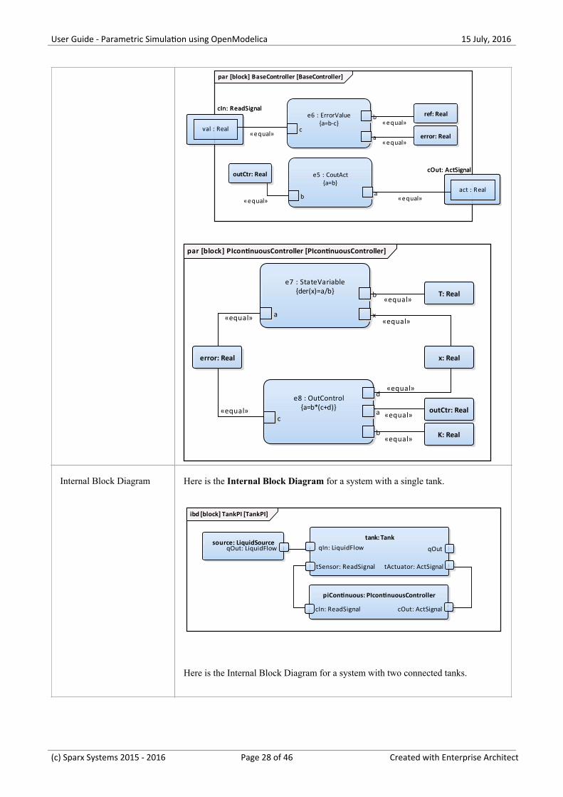
The Constrains defined for BaseController and PIcontinuousController areillustrated in the following figures.
(c) Sparx Systems 2015 - 2016 Page 27 of 46 Created with Enterprise Architect
User Guide - Parametric Simulation using OpenModelica 15 July, 2016
cIn: ReadSignal
cOut: ActSignal
par [block] BaseController [BaseController]
cIn: ReadSignal
cOut: ActSignale5 : CoutAct
{a=b}
e6 : ErrorValue{a=b-c}
ab
a
b
cerror: Real
outCtr: Real
ref: Real
val : Real
act : Real
«equal»
«equal»
«equal»
«equal»
«equal»
par [block] PIcontinuousController [PIcontinuousController]
e7 : StateVariable{der(x)=a/b}
e8 : OutControl{a=b*(c+d)}
xa
K: Real
b
a
b
c
d
x: Real
T: Real
error: Real
outCtr: Real
«equal»
«equal»
«equal»
«equal»
«equal»«equal»
«equal»
Internal Block Diagram Here is the Internal Block Diagram for a system with a single tank.
ibd [block] TankPI [TankPI]
qOut: LiquidFlowsource: LiquidSource
qOut: LiquidFlow
cIn: ReadSignal cOut: ActSignal
piContinuous: PIcontinuousController
cIn: ReadSignal cOut: ActSignal
qOutqIn: LiquidFlow
tSensor: ReadSignal tActuator: ActSignal
tank: Tank
qOutqIn: LiquidFlow
tSensor: ReadSignal tActuator: ActSignal
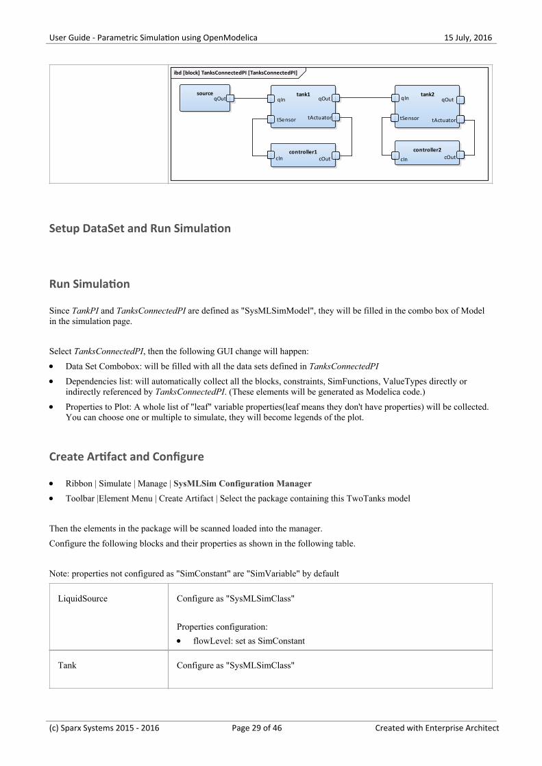
Here is the Internal Block Diagram for a system with two connected tanks.
(c) Sparx Systems 2015 - 2016 Page 28 of 46 Created with Enterprise Architect
User Guide - Parametric Simulation using OpenModelica 15 July, 2016
ibd [block] TanksConnectedPI [TanksConnectedPI]
tSensor tActuator
qOutqIntank1
tSensor tActuator
qOutqIn
tSensor tActuator
qOutqIntank2
tSensor tActuator
qOutqIn
cOutcIncontroller1
cOutcIn cOutcIn
controller2cOutcIn
qOutsource
qOut
Setup DataSet and Run Simulation
Run Simulation
Since TankPI and TanksConnectedPI are defined as "SysMLSimModel", they will be filled in the combo box of Modelin the simulation page.
Select TanksConnectedPI, then the following GUI change will happen:
Data Set Combobox: will be filled with all the data sets defined in TanksConnectedPI·Dependencies list: will automatically collect all the blocks, constraints, SimFunctions, ValueTypes directly or·indirectly referenced by TanksConnectedPI. (These elements will be generated as Modelica code.)
Properties to Plot: A whole list of "leaf" variable properties(leaf means they don't have properties) will be collected.·You can choose one or multiple to simulate, they will become legends of the plot.
Create Artifact and Configure
Ribbon | Simulate | Manage | SysMLSim Configuration Manager·Toolbar |Element Menu | Create Artifact | Select the package containing this TwoTanks model·
Then the elements in the package will be scanned loaded into the manager.
Configure the following blocks and their properties as shown in the following table.
Note: properties not configured as "SimConstant" are "SimVariable" by default
LiquidSource Configure as "SysMLSimClass"
Properties configuration:
flowLevel: set as SimConstant·
Tank Configure as "SysMLSimClass"
(c) Sparx Systems 2015 - 2016 Page 29 of 46 Created with Enterprise Architect
User Guide - Parametric Simulation using OpenModelica 15 July, 2016
Properties configuration:
area: set as SimConstant·flowGain: set as SimConstant·maxV: set as SimConstant·minV: set as SimConstant·
BaseController Configure as "SysMLSimClass"
Properties configuration:
K: set as SimConstant·T: set as SimConstant·Ts: set as SimConstant·ref: set as SimConstant·
PIcontinuousController Configure as "SysMLSimClass"
TankPI Configure as "SysMLSimModel"
TanksConnectedPI Configure as "SysMLSimModel"
Setup DataSet
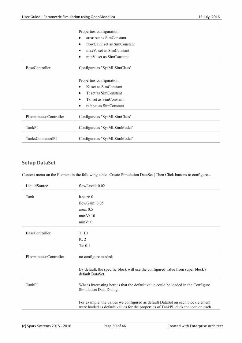
Context menu on the Element in the following table | Create Simulation DataSet | Then Click buttons to configure...
LiquidSource flowLevel: 0.02
Tank h.start: 0
flowGain: 0.05
area: 0.5
maxV: 10
minV: 0
BaseController T: 10
K: 2
Ts: 0.1
PIcontinuousController no configure needed;
By default, the specific block will use the configured value from super block'sdefault DataSet.
TankPI What's interesting here is that the default value could be loaded in the ConfigureSimulation Data Dialog.
For example, the values we configured as default DataSet on each block elementwere loaded as default values for the properties of TankPI, click the icon on each
(c) Sparx Systems 2015 - 2016 Page 30 of 46 Created with Enterprise Architect
User Guide - Parametric Simulation using OpenModelica 15 July, 2016
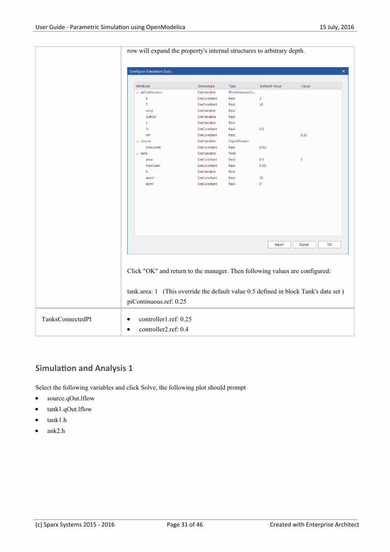
row will expand the property's internal structures to arbitrary depth.
Click "OK" and return to the manager. Then following values are configured:
tank.area: 1 (This override the default value 0.5 defined in block Tank's data set )
piContinuous.ref: 0.25
TanksConnectedPI controller1.ref: 0.25·controller2.ref: 0.4·
Simulation and Analysis 1
Select the following variables and click Solve, the following plot should prompt
source.qOut.lflow·tank1.qOut.lflow·tank1.h·ank2.h·
(c) Sparx Systems 2015 - 2016 Page 31 of 46 Created with Enterprise Architect
User Guide - Parametric Simulation using OpenModelica 15 July, 2016
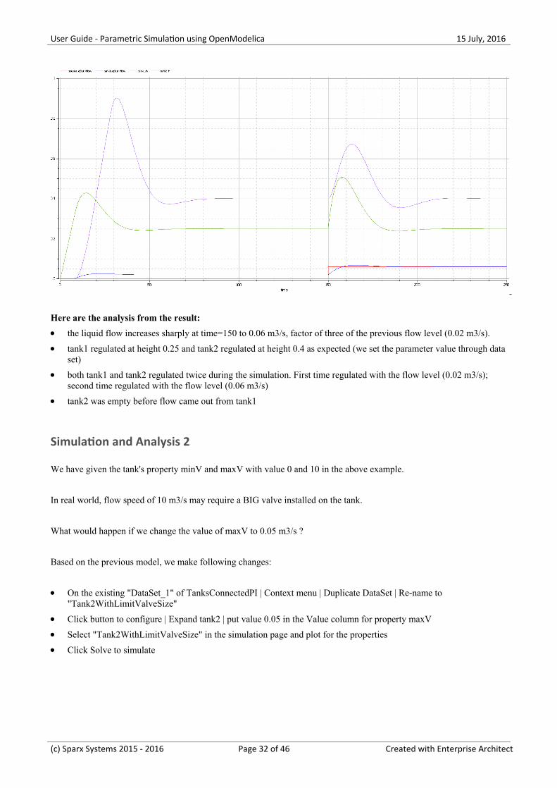
Here are the analysis from the result:
the liquid flow increases sharply at time=150 to 0.06 m3/s, factor of three of the previous flow level (0.02 m3/s).·tank1 regulated at height 0.25 and tank2 regulated at height 0.4 as expected (we set the parameter value through data·set)
both tank1 and tank2 regulated twice during the simulation. First time regulated with the flow level (0.02 m3/s);·second time regulated with the flow level (0.06 m3/s)
tank2 was empty before flow came out from tank1·
Simulation and Analysis 2
We have given the tank's property minV and maxV with value 0 and 10 in the above example.
In real world, flow speed of 10 m3/s may require a BIG valve installed on the tank.
What would happen if we change the value of maxV to 0.05 m3/s ?
Based on the previous model, we make following changes:
On the existing "DataSet_1" of TanksConnectedPI | Context menu | Duplicate DataSet | Re-name to·"Tank2WithLimitValveSize"
Click button to configure | Expand tank2 | put value 0.05 in the Value column for property maxV·Select "Tank2WithLimitValveSize" in the simulation page and plot for the properties·Click Solve to simulate·
(c) Sparx Systems 2015 - 2016 Page 32 of 46 Created with Enterprise Architect
User Guide - Parametric Simulation using OpenModelica 15 July, 2016
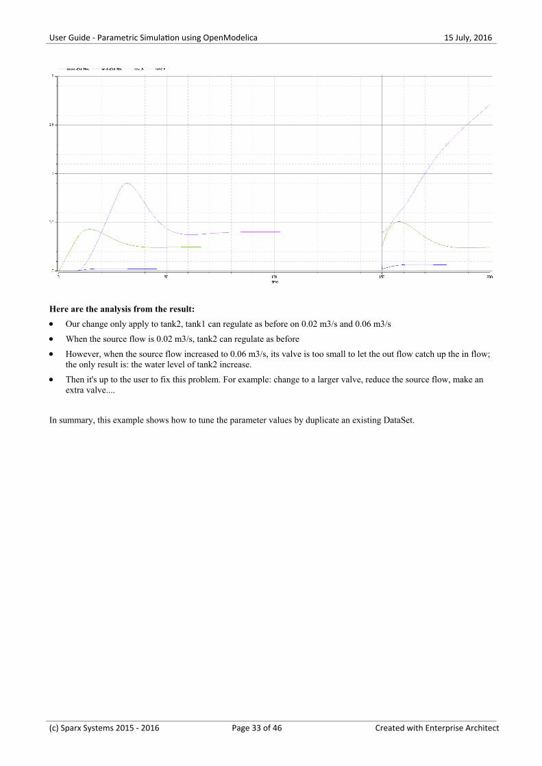
Here are the analysis from the result:
Our change only apply to tank2, tank1 can regulate as before on 0.02 m3/s and 0.06 m3/s·When the source flow is 0.02 m3/s, tank2 can regulate as before·However, when the source flow increased to 0.06 m3/s, its valve is too small to let the out flow catch up the in flow;·the only result is: the water level of tank2 increase.
Then it's up to the user to fix this problem. For example: change to a larger valve, reduce the source flow, make an·extra valve....
In summary, this example shows how to tune the parameter values by duplicate an existing DataSet.
(c) Sparx Systems 2015 - 2016 Page 33 of 46 Created with Enterprise Architect
User Guide - Parametric Simulation using OpenModelica 15 July, 2016
Creating a Parametric Model
When creating a Parametric Model, you can apply one of three approaches to defining Constraint Equations:
Defining inline Constraint Equations on a Block element·Creating re-usable Constraint Blocks, and·Using connected constraint properties·
You would also take into consideration:
Flows in physical interactions·Default Values and Initial Values·Simulation Functions·Value Allocation, and·Packages and Imports·
Access
Ribbon Simulate > SysMLSim > Manage > SysMLSim Configuration Manager
Defining inline Constraint Equations on a Block
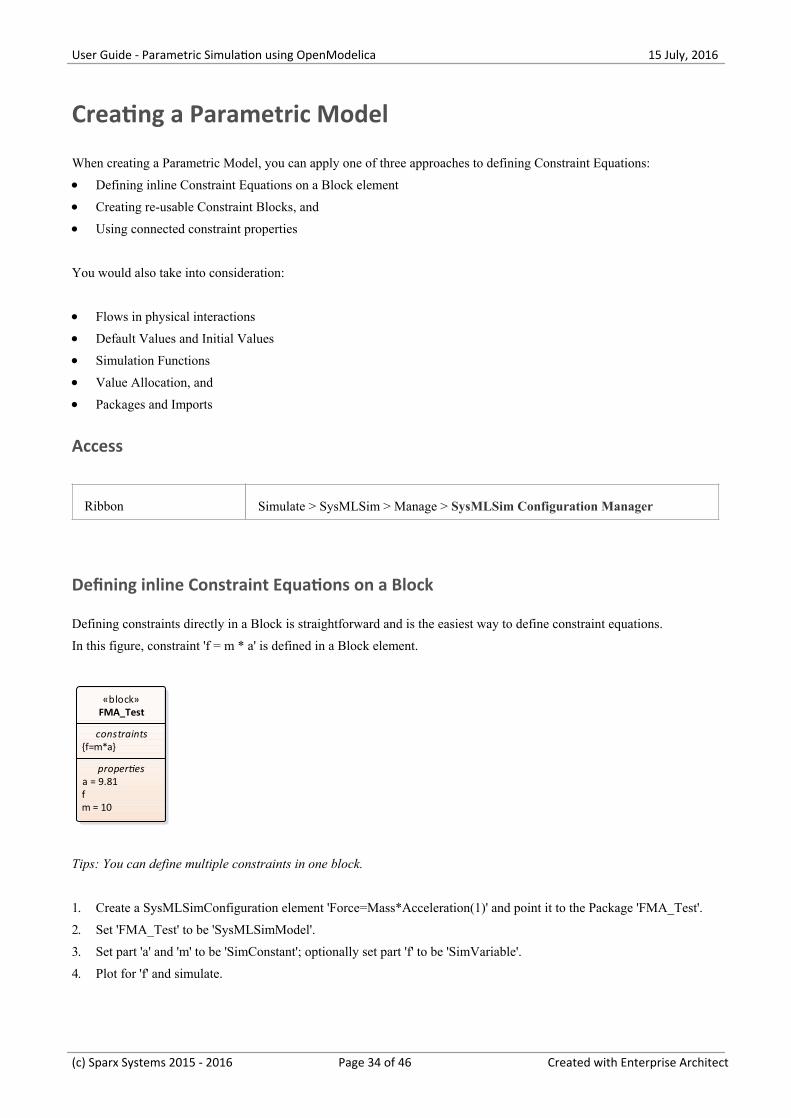
Defining constraints directly in a Block is straightforward and is the easiest way to define constraint equations.
In this figure, constraint 'f = m * a' is defined in a Block element.
«block»FMA_Test
constraints{f=m*a}
properties a = 9.81 f m = 10
Tips: You can define multiple constraints in one block.
Create a SysMLSimConfiguration element 'Force=Mass*Acceleration(1)' and point it to the Package 'FMA_Test'.1.
Set 'FMA_Test' to be 'SysMLSimModel'.2.
Set part 'a' and 'm' to be 'SimConstant'; optionally set part 'f' to be 'SimVariable'.3.
Plot for 'f' and simulate.4.
(c) Sparx Systems 2015 - 2016 Page 34 of 46 Created with Enterprise Architect
User Guide - Parametric Simulation using OpenModelica 15 July, 2016
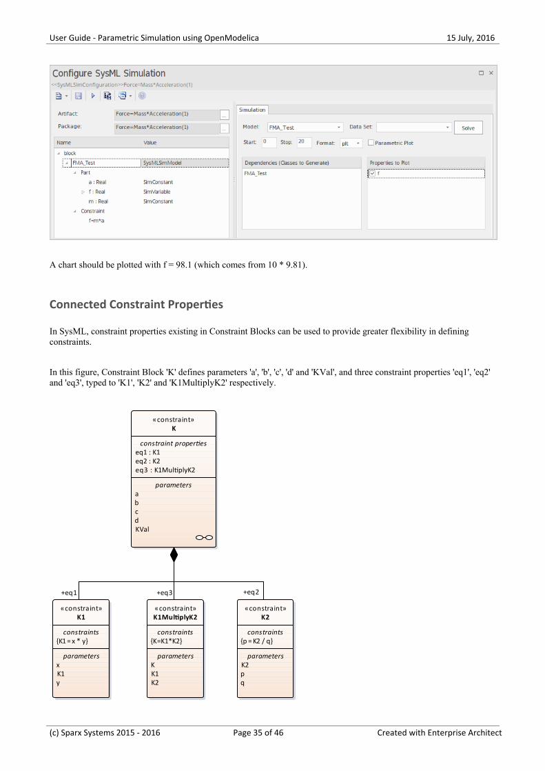
A chart should be plotted with f = 98.1 (which comes from 10 * 9.81).
Connected Constraint Properties
In SysML, constraint properties existing in Constraint Blocks can be used to provide greater flexibility in definingconstraints.
In this figure, Constraint Block 'K' defines parameters 'a', 'b', 'c', 'd' and 'KVal', and three constraint properties 'eq1', 'eq2'and 'eq3', typed to 'K1', 'K2' and 'K1MultiplyK2' respectively.
«constraint»K2
constraints{p = K2 / q}
parameters K2 p q
«constraint»K1
constraints{K1 = x * y}
parameters x K1 y
«constraint»K1MultiplyK2
constraints{K=K1*K2}
parameters K K1 K2
«constraint»K
constraint properties eq1 : K1 eq2 : K2 eq3 : K1MultiplyK2
parameters a b c d KVal
+eq3+eq1 +eq2
(c) Sparx Systems 2015 - 2016 Page 35 of 46 Created with Enterprise Architect

User Guide - Parametric Simulation using OpenModelica 15 July, 2016
Create a Parametric diagram in Constraint Block 'K' and connect the parameters to the constraint properties with bindingconnectors, as shown:
par [constraint block] K [K]
eq3 : K1MultiplyK2{K=K1*K2}
K1 K2
K
eq2 : K2{p = K2 / q}
p
qK2eq1 : K1
{K1 = x * y}
x
yK1
KVal
d
c
b
a
«equal»
«equal»
«equal»
«equal»
«equal»
«equal»
«equal»
Create a model MyBlock with five Properties (Parts)·Create a constraint property 'eq' for MyBlock and show the parameters·Bind the properties to the parameters·
par [block] MyBlock [MyBlockPar]
arg_b
arg_a
arg_K
arg_d
arg_c
eq : K
KVal
d
c
b
a«equal»
«equal»
«equal»
«equal»
«equal»
Provide values (arg_a = 2, arg_b = 3, arg_c = 4, arg_d = 5) in a data set·In the 'Configure SysML Simulation' dialog, select MyBlock > DataSet_1 and plot for 'arg_K', and run the·simulation
(c) Sparx Systems 2015 - 2016 Page 36 of 46 Created with Enterprise Architect

User Guide - Parametric Simulation using OpenModelica 15 July, 2016
The result 120 (calculated as 2 * 3 * 4 * 5) will be computed and plotted. This is the same as when we do an expansionwith pen and paper: K = K1 * K2 = (x*y) * (p*q), then bind with the values (2 * 3) * (4 * 5); we get 120.
What is interesting here is that we intentionally define K2's equation to be 'p = K2 / q' and this example still works.
We can easily solve K2 to be p * q in this example, but in some complex examples it is extremely hard to solve avariable from an equation; however, the EA SysMLSim can still get it right.
In summary, the example shows you how to define a Constraint Block with greater flexibility by constructing theconstraint properties. Although we demonstrated only one layer down into the constraint block, this mechanism couldwork on complex models for an arbitrary level of use.
Creating Reuseable Constraint Blocks
If one equation is commonly used in many Blocks, a Constraint Block can be created for use as a constraint property ineach Block. These are the changes we make, based on the previous example:
Create a Constraint Block element 'F_Formula' with three parameters 'a', 'm' and 'f', and a constraint 'f = m * a·
(c) Sparx Systems 2015 - 2016 Page 37 of 46 Created with Enterprise Architect

User Guide - Parametric Simulation using OpenModelica 15 July, 2016
Tip: Primitive type 'Real' will be applied if property types are empty
Create a Block 'FMA_Test' with three properties 'x', 'y' and 'z', and give 'x' and 'y' the default values '10' and '9.81'·respectively
Create a Parametric diagram in 'FMA_Test', showing the properties 'x', 'y' and 'z'·Create a 'Constraint Property' 'e1' typed to 'F_Formula' and show the parameters·Draw binding connectors between 'x—m', 'y—a', and 'f—z' as shown:·
par [block] FMA_Test [testingFormulaF]
e1 : F_Formula{f=m*a}
a
mf z
y
x
«equal»«equal»
«equal»
Create a SysMLSimConfiguration Artifactelement and configure it like this: - Set 'FMA_Test' to be 'SysMLSimModel' - Set 'x' and 'y' to be 'SimConstant' - Plot for 'z' and simulate
(c) Sparx Systems 2015 - 2016 Page 38 of 46 Created with Enterprise Architect

User Guide - Parametric Simulation using OpenModelica 15 July, 2016
A chart should be plotted with f = 98.1 (which comes from 10 * 9.81).
Flows in Physical Interactions
When modeling for physical interaction, exchanges of conserved physical substances such as electrical current, force,torque and flow rates hould be modeled as flows and the attribute 'isConserved' should be set on the flow variables.
Two different types of coupling are established by connections, depending on whether the flow properties are potential(default) or flow (conserved):
Equality coupling, for potential (also called effort) properties·Sum-to-zero coupling, for flow (conserved) properties; for example, according to Kirchoff's current law in the·electrical domain, conservation of charge makes all charge flows into a point sum to zero
In the generated Modelica code of the 'ElectricalCircuit' example:
connector ChargePort
flow Current i; //flow keyword will be generated if 'isConserved' = true
Voltage v;
end ChargePort;
model Circuit
Source source;
Resistor resistor;
Ground ground;
equation
connect(source.p, resistor.n);
connect(ground.p, source.n);
connect(resistor.p, source.n);
end Circuit;
Each connect equation is actually expanded to two equations (there are two properties defined in ChargePort), one forequality coupling, the other for sum-to-zero coupling:
source.p.v = resistor.n.v;
source.p.i + resistor.n.i = 0;
Default Value and Initial Values
If initial values are defined in SysML property elements (Properties dialog > Property page > 'Initial' field), they can beloaded as the default value for SimConstant or the initial value for SimVariable.
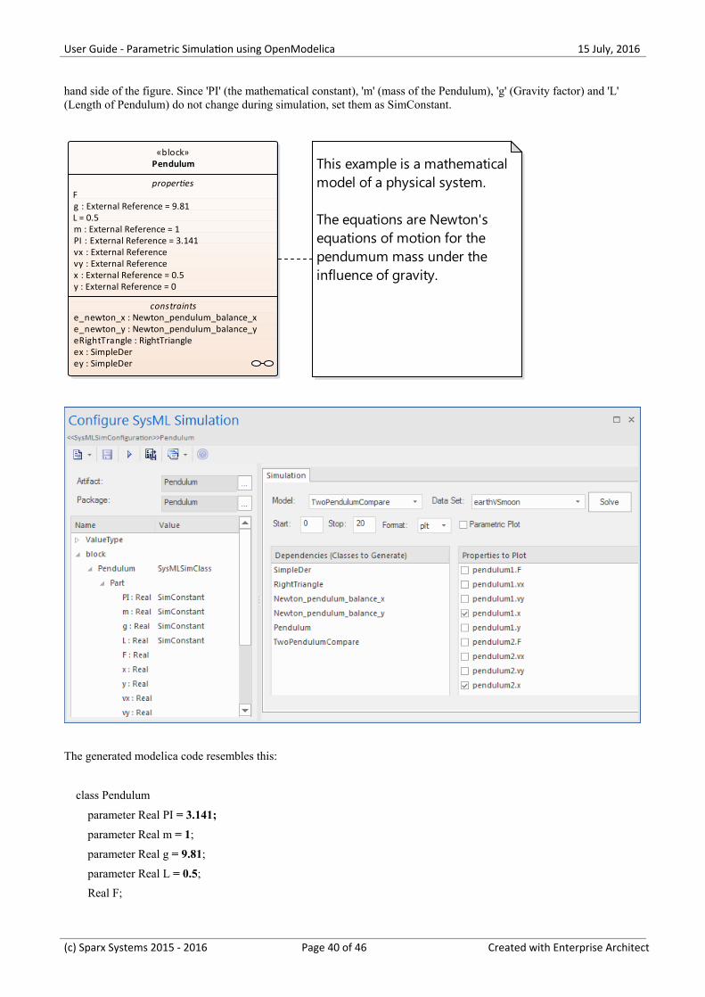
In this Pendulum example, we have provided initial values for properties 'g', 'L', 'm', 'PI', 'x' and 'y', as seen on the left
(c) Sparx Systems 2015 - 2016 Page 39 of 46 Created with Enterprise Architect
User Guide - Parametric Simulation using OpenModelica 15 July, 2016
hand side of the figure. Since 'PI' (the mathematical constant), 'm' (mass of the Pendulum), 'g' (Gravity factor) and 'L'(Length of Pendulum) do not change during simulation, set them as SimConstant.
«block»Pendulum
properties F g : External Reference = 9.81 L = 0.5 m : External Reference = 1 PI : External Reference = 3.141 vx : External Reference vy : External Reference x : External Reference = 0.5 y : External Reference = 0
constraints e_newton_x : Newton_pendulum_balance_x e_newton_y : Newton_pendulum_balance_y eRightTrangle : RightTriangle ex : SimpleDer ey : SimpleDer
This example is a mathematical model of a physical system.
The equations are Newton's equations of motion for the pendumum mass under the influence of gravity.
The generated modelica code resembles this:
class Pendulum
parameter Real PI = 3.141;
parameter Real m = 1;
parameter Real g = 9.81;
parameter Real L = 0.5;
Real F;
(c) Sparx Systems 2015 - 2016 Page 40 of 46 Created with Enterprise Architect

User Guide - Parametric Simulation using OpenModelica 15 July, 2016
Real x (start=0.5);
Real y (start=0);
Real vx;
Real vy;
......
equation
......
end Pendulum;
Properties 'PI', 'm', 'g' and 'L' are constant, and are generated as a declaration equation·Properties 'x' and 'y' are variable; their starting values are 0.5 and 0 respectively, and the initial values are generated·as modifications
Simulation Functions
A Simulation function is a powerful tool for writing complex logic, and is easy to use for constraints. This sectiondescribes a function from the TankPI example.
In the Constraint Block 'Q_OutFlow', a function 'LimitValue' is defined and used in the constraint.
«constraint»Q_OutFlow
«SimFunction»+ LimitValue(double, double, double, double*): int
constraints{a=LimitValue(min, max, -b*c)}
parameters a b c max min
On a Block or Constraint Block, create an operation ('LimitValue' in this example) and open the 'Operations' tab of·the 'Features' dialog.
Give the operation the stereotype 'SimFunction'·Define the parameters and set the direction to 'in/out'·
Tips: Multiple parameters could be defined as 'out', and the caller retrieves the value in format of:
(out1, out2, out3) = function_name(in1, in2, in3, in4, ...); //Equation form
(out1, out2, out3) := function_name(in1, in2, in3, in4, ...); //Statement form
Define the function body in the 'Initial Code' field of the 'Behavior' tab·
The function body is defined as shown:
(c) Sparx Systems 2015 - 2016 Page 41 of 46 Created with Enterprise Architect

User Guide - Parametric Simulation using OpenModelica 15 July, 2016
pLim :=
if p > pMax then
pMax
else if p< pMin then
pMin
else
p;
When generating code, Enterprise Architect will collect all the operations stereotyped as 'SimFunction' defined inConstraint Blocks and Blocks, then generate code resembling this:
function LimitValue
input Real pMin;
input Real pMax;
input Real p;
output Real pLim;
algorithm
pLim :=
if p > pMax then
pMax
else if p< pMin then
pMin
else
p; end LimitValue;
Value Allocation
This figure shows a simple model called 'Force=Mass*Accelaration'.
«constraint»F_Formula
constraints{f=m*a}
parameters a f m
«block»FMA
properties a f m
constraints e1 : F_Formula
«block»FMA_Test
constraints{a_value=sin(time)}{m_value=cos(time)}
properties a_value fma1 : FMA m_value
A block 'FMA' is modeled with properties 'a', 'f', and 'm' and a constraintProperty 'e1', typed to Constraint Block·'F_Formula'
The block 'FMA' does not have any initial value set on its properties, and the properties 'a', 'f' and 'm' are all variable,·
(c) Sparx Systems 2015 - 2016 Page 42 of 46 Created with Enterprise Architect

User Guide - Parametric Simulation using OpenModelica 15 July, 2016
so their value change depends on the environment in which they are simulated
Create a block 'FMA_Test' as SysMLSimModel and add the property 'fma1' to test the behavior of block 'FMA'·Constraint 'a_value' to be 'sin(time)'·Constraint 'm_value' to be 'cos(time)'·Draw Allocation connectors to allocate values from environment to the model 'FMA'·
ibd [block] FMA_Test [FMA_Test]
value constraint as "sin(time)"
value constraint as"cos(time)"
a_value
fma1: FMA
a
m m_value«a llocate»
«a llocate»
Plot for 'fma1.a', 'fma1.m', 'fma1.f' and simulate the model·
Packages and Imports
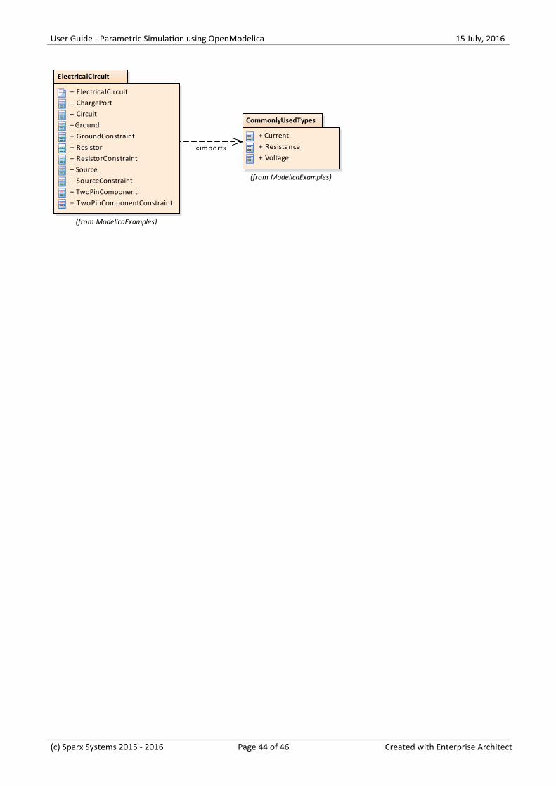
The SysMLSimConfiguration Artifact collects the elements (such as Blocks, Constraint Blocks and Value Types) of aPackage. If the simulation depends on elements not owned by this Package, such as Reusable libraries, EnterpriseArchitect provides an Import connector between Package elements to meet this requirement.
In the Electrical Circuit example, the Artifact is configured to the Package 'ElectricalCircuit', which contains almost allof the elements needed for simulation. However, some properties are typed to value types such as 'Voltage', 'Current' and'Resistance', which are commonly used in multiple SysML models and placed in a Package called 'CommonlyUsedTypes'outside the individual SysML models. If you import this Package using an Import connector, all the elements in theimported Package will appear in the SysMLSim Configuration Manager.
(c) Sparx Systems 2015 - 2016 Page 43 of 46 Created with Enterprise Architect
User Guide - Parametric Simulation using OpenModelica 15 July, 2016
ElectricalCircuit
+ ElectricalCircuit+ ChargePort+ Circuit+ Ground+ GroundConstraint+ Resistor+ ResistorConstraint+ Source+ SourceConstraint+ TwoPinComponent+ TwoPinComponentConstraint
(from ModelicaExamples)
CommonlyUsedTypes
+ Current+ Resistance+ Voltage
(from ModelicaExamples)
«import»
(c) Sparx Systems 2015 - 2016 Page 44 of 46 Created with Enterprise Architect
User Guide - Parametric Simulation using OpenModelica 15 July, 2016
Troubleshooting OpenModelica Simulation
Common Simulation Issues
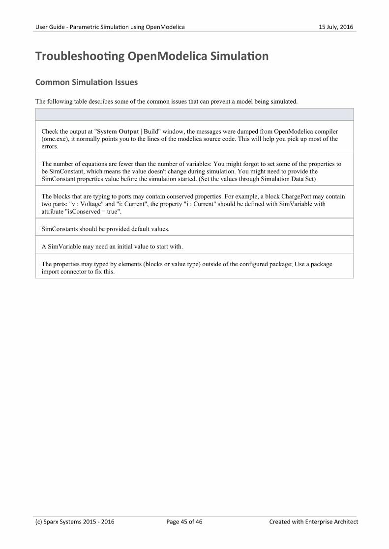
The following table describes some of the common issues that can prevent a model being simulated.
Check the output at "System Output | Build" window, the messages were dumped from OpenModelica compiler(omc.exe), it normally points you to the lines of the modelica source code. This will help you pick up most of theerrors.
The number of equations are fewer than the number of variables: You might forgot to set some of the properties tobe SimConstant, which means the value doesn't change during simulation. You might need to provide theSimConstant properties value before the simulation started. (Set the values through Simulation Data Set)
The blocks that are typing to ports may contain conserved properties. For example, a block ChargePort may containtwo parts: "v : Voltage" and "i: Current", the property "i : Current" should be defined with SimVariable withattribute "isConserved = true".
SimConstants should be provided default values.
A SimVariable may need an initial value to start with.
The properties may typed by elements (blocks or value type) outside of the configured package; Use a packageimport connector to fix this.
(c) Sparx Systems 2015 - 2016 Page 45 of 46 Created with Enterprise Architect
User Guide - Parametric Simulation using OpenModelica 15 July, 2016
(c) Sparx Systems 2015 - 2016 Page 46 of 46 Created with Enterprise Architect
Top Related