


Languages
Pages
Legal

presented at the Weimar Optimization and Stochastic Days 2016
Source: www.dynardo.de/en/library
Lectures
Optimization of Hydrocarbon
Production from Unconventional
Shale Reservoirs using FEM
based fracture simulation
J. Will, St. Eckardt

page 1
Optimization of Hydrocarbon Production from Unconventional Shale Reservoirs
using FEM based fracture simulation
Johannes Will, Stefan Eckardt: Dynardo GmbH
1 Introduction
Substantial quantities of oil and gas are currently being produced from Unconventional Resources /
Reservoirs. These reservoirs are usually characterized by high shale content and ultra-low matrix
permeabilities. Most completions in Unconventional Reservoirs are hydraulically fracture stimulated
in order to establish a more effective flow from the far-field reservoir and fracture network to the
wellbore. The success of hydraulic fracture stimulation in horizontal wells has resulted in it being
ranked as one of the major distinguishing technologies of the 21st Century. It has already realized its
potential to dramatically change the oil and gas production landscape across the globe, and the impact
will endure for decades to come.
For a given field development project, the derived economics is highly dependent on the effectiveness
of the drilling and completion operation to establish effective and retained contact with the
hydrocarbon resource. This paper introduces a suggested process to model, calibrate, and optimize the
landing of the well and the optimization of the hydraulic fracture stimulation design for naturally
fractured reservoirs.
The introduced workflow combines the commercial software packages ANSYS® [1] and multiPlas [2]
within a 3D Hydraulic Fracturing Simulator [3] for the parametric Finite Element (FEM) Modeling
and material modeling of naturally fractured sedimentary rocks. With the utility of optiSLang® [4],
automated sensitivity studies of the uncertainty of reservoir, engineering, and operational parameters
are performed and are evaluated relative to the resulting Stimulated Reservoir Volume (SRV) and
Accessible Hydrocarbon Resource. Results from these studies are then used to optimize the well
placements and completion designs.
Unlike most academic and commercial approaches, the introduced approach uses a homogenized
continuum approach to model the 3D hydraulic fracturing in naturally fractured reservoirs. The
principal motivation for using a continuum approach is the numerical efficiency necessary to run fully
3D coupled hydraulic/mechanical simulations of the hydraulic fracturing of multiple stages and
multiple wells in naturally fractured sedimentary rocks. A fully 3D discrete fracture simulator
respective of Mohr-Coulomb failure is numerically quite intensive. A discrete fracture model has not
yet been developed using a fully 3D explicit fracture growth modeling system.
Hydraulic fracturing in shale reservoirs is mostly dominated by the anisotropic stress and strength
conditions resulting from the initial patterns of planes of weakness, these usually being the natural
joints and fractures of the source rock. To capture this impact on fracture mechanics, the three-
dimensional modeling of anisotropic strength, stress, and conductivity of the matrix and of the fracture
system is required. Simulation simplification to 2D or pseudo-3D geometric modeling will fail to
capture the effects necessary to properly model the potentially most important effects which may drive
the hydraulic fracturing process and the resulting production performance.
The homogenized continuum approach was initially developed and applied in the Civil Engineering
field of Waterway and Dam Engineering to better determine the influence of water flow in naturally
fractured dam foundations [5]. It was improved and generalized for the coupled hydraulic-mechanical
simulation of naturally fractured rocks using commercial FEM codes [6]. These developments provide
page 2
the basis for the software tool “multiPlas” [2], which provides for the non-linear modeling of jointed
rocks.
The introduced workflow is an integrated well placement and completion design optimization
workflow. The toolkit integrates geo-mechanical descriptions, formation characterizations, flow
dynamics, microseismic event catalogues, hydraulic fracturing monitoring data, well completion and
operational parameters in a modeling environment with optimization capability. It is built upon a 3D
geological model with multi-disciplinary inputs including formation properties, in-situ stresses, natural
fracture descriptions, and well and completion parameters (i.e., well orientation, landing interval, fluid
rate and volume, perforation spacing, and stage spacing). Upon calibrating with the hydraulic
fracturing field observations, the introduced workflow optimized well completion design, and
guidance on data acquisition and diagnostic needs to achieve EUR performance at optimized costs.
1.1 Background on Dynardo’s Hydraulic Fracturing Modeling Approach
The inherent anisotropies of unconventional reservoirs result from layering, deformation history,
strength and stress variability, and the non-uniform conductivity of the fractured rock mass. Because
of these complexities, hydraulic fracturing should be simulated in a fully three-dimensional coupled
hydro-mechanical model. Most shale hydrocarbon resources are essentially jointed even before
hydraulic fracturing takes place. These planes of weakness include the bedding plane and usually two
or three additional sets of natural planes of weakness.
Most commercial hydraulic fracture simulators model hydraulic fracturing using 1D, 2D, or pseudo
3D geometric approaches. In many cases, these simplifications prevent the simulators from adequately
modeling the complex hydraulic fracturing mechanisms that are present. This may dramatically
oversimplify the simulated fracture geometry, and may fail to identify the opportunities for economic
production improvement in all but the most trivial of shale resource settings [7].
For a fully 3D modeling approach, achieving an effective numerical discretization capable of
representing multiple stages and multiple wells in a complex reservoir setting is necessary. A discrete
modeling approach of natural fractures or a homogenized modeling approach of fractures can be
developed. However, the discrete modeling of a network of joints resulting from the hydraulic
fracturing of the rock mass is currently computationally “extraordinarily expensive” to the point of
impracticality for wellbore-scale models. Such models include discrete element and particle
approaches (DEM, Particle codes) or discrete fracture modeling in continuum mechanics approaches
(XFEM, cohesive zone elements). Currently, there are no commercial simulation solutions available
for the wellbore-scale fully 3D hydraulic fracturing simulation of multiple stages and multiple wells
using discrete joint modeling. Although a majority of research groups are following discrete fracture
modeling approaches, a fully 3D discrete solution appears elusive at the needed wellbore-scale.
The modeling of coupled hydro-mechanical problems in rock mechanics using a homogenized
continuum strategy was successfully implemented for science and industrial applications by Wittke [5]
and others in the 1980s and 1990s. The weak point of the numerical implementation at that time was
the inability of consistent integration of multi-surface plasticity, which is a result of dealing with
multiple yield criteria at the material point level in the homogenized continuum representing intact
rock (matrix) and multiple joint sets. To overcome the problem, Wittke introduced a pseudo-viscous
numerical procedure which depended on pseudo-parameters which had a seemingly unreasonable
influence on the results. Using a homogenized modeling approach for jointed rock in implicit
integration algorithms resulted in convergence difficulties. Science groups moved to trial explicit time
page 3
integration procedures using discrete modeling techniques or particle based models. Here convergence
problems are minimal. However, because of the stability requirements of explicit time integration
schemes, these approaches became computationally “extraordinarily” time consuming when modeling
transient 3D wellbore scale problems.
After attempting discrete joint modeling and explicit time integration methods for several years,
researchers at the Bauhaus University in the late 90’s returned to a homogenized continuum approach,
and developed a solution for the problem of consistent integration of multi-surface plasticity using
implicit time integration [6]. As a result, hydraulic fracturing can now be efficiently modeled by using
implicit finite element formulations, incorporating real world fully 3D reservoir conditions including
all relevant anisotropies and thermo-hydro-mechanical coupling [8].
1.2 Every Hydraulic Fracturing Simulator Needs to be Calibrated for Typical
Reservoir Conditions
A practical 3D Hydraulic Fracturing Simulator that could simulate multiple stages in multiple wells
with reasonable numerical effort was now available. The challenge was then to properly characterize
the geomechanical (stress, strengths, moduli, cohesion, friction angle, YM, PR, etc.) and the hydraulic
(pressure, saturations, compressibility, permeability, etc.) setting of the resource. It is a formidable
task to accurately measure the total state of the reservoir and bounding layers. However, in order to
model realistic fracture height growths, all relevant potential fracture barriers need to be modeled and
parameterized. Significant fracture barriers may occur due to layered contrast in deformation, stress,
and strength characteristics. Similarly, faults and previously created hydraulic fractures may act as
preferred mechanisms for fracture growth. These are generally to be expected when horizontal well
fracture stimulations are closely staged.
After constructing a layered reservoir and bounding rock model inclusive of the potential fracture
barriers, the calibration of large amounts of uncertain rock parameters to the best available
measurements was necessary. A parameter identification problem exists simply because of the large
number (>100) of model parameters, and they may have a considerable associated uncertainly. During
the calibration phase, the workflow applies optiSlang [4], a commercial tool box for variation space
management and optimization analysis. The process involves running a set of calibration models
respective of the variation space of the model. With optiSLang, all parameters in a parametric
hydraulic fracturing model can be identified and updated efficiently for successive model runs, which
are then initialized and executed in an automated process. A large number of calibration sensitivity
design runs can be executed in a comparatively short period of time.
The calibration phase ideally requires quality data measurements. This includes the pressure
measurements that are used to derive ISIP/DFIT (Instantaneous Shut-In Pressure, Dynamic Fracture
Intensity Test) conditions as well as the projected bottom-hole pressure history. The representative
microseismic event catalog is also used in the calibration phase. Uncertainty analysis is integrated in
the calibration process to better identify the most influential parameters controlling fracture geometry.
This calibration process also provides the potential to focus additional data gathering to those
parameters that significantly affect the simulation results.
Once a calibrated model is developed that is respecting of the resource data as well as the
microseismic event data, the simulator can then be used in a forecast mode to better optimize the well
landing depth and the completion design.

page 4
1.3 What is the Right Value to be Optimized?
After having a 3D Hydraulic Fracturing Simulator that is well calibrated to the reservoir, the next
question is “What are the right quantities to optimize?” Conventionally, Stimulated Rock Volume
(SRV) is used to quantify the effectiveness of the fracture stimulation. SRV variation is clearly
dominated by fluid volume variation: more frac fluid simply creates more fractures and more frac
volume. The simulation results can be used to fully quantify which reservoir layers are being
fractured, how much frac height and frac length is produced, which fractures accepts proppant based
on apertures, and how the created fracture network might effectively drain the reservoir.
First, only created fractures that are acceptant of proppant with sustained connectivity to at least one
perforation cluster or flow port are credited with production potential. The related proppant-accepting
volume is referred to as Valuable SRV (VSRV). Second, the drainage volume over the productive
life of the well is calculated based on the VSRV with consideration for an average drainage radius. By
integration of the pore and hydrocarbon content in the reservoir layers over the drainage volume, the
Accessible Hydrocarbon Initially In Place (AHCIIP) can be calculated. This represents the
producible hydrocarbons connected to the wellbore. By applying a representative recovery factor, the
estimated hydrocarbon production expected over the lifetime of the well is calculated. The economic
maximization of AHCIIP is usually the optimization goal.
A very important verification of the forecast quality of the calibrated reservoir model is the
comparison of the estimated hydrocarbon production from the hydraulic fracturing simulator to
Estimated Ultimate Recovery (EUR) of the calibration well and neighboring wells.
Fig. 1-1 worklow for optimization of hydrocarbon production in unconventional oil and gas
reservoir
page 5
During the optimization procedure, the major completion parameters such as well orientation, landing
depth, stage design, well spacing, and fluid volume will generally be the most influential parameters.
The optimization process is usually a compromise between increasing EUR potential subject to
reducing completion costs. This optimization is represented by a classic Pareto Frontier. Using
optiSLang, the Pareto Frontier represents the design limits where any production improvement cannot
be introduced anymore without increasing the completion costs. The Pareto Frontier is the final result
of the workflow. It is used for rationalizing the decision between maximizing AHCIIP and minimizing
the related completion costs.
2 The Dynardo Hydraulic Fracturing Simulator
The Hydraulic Fracturing Simulator [3] combines three commercial software packages: ANSYS® [1],
multiPlas [2] and optiSLang® [4]. ANSYS is used for the development of parametric reservoir finite
element models. The coupled hydraulic-mechanical analysis is performed with ANSYS. The second
module, multiPlas, is an ANSYS extension for non-linear material modeling. These material models
extend the ANSYS functionality to the non-linear mechanical analysis of naturally fractured rocks.
Within the context of the hydraulic fracturing simulator, multiPlas additionally provides an anisotropic
hydraulic element which models the flow through fractured rock. The third software product,
optiSLang, is used to efficiently calibrate the model and to perform sensitivity analyses in
consideration of the uncertainties in the reservoir model and operational conditions.
In order to reach a sufficient forecast quality in the simulation of hydraulic fracturing, the most
important phenomena that needs to be represented by the model is the three-dimensional anisotropic
strength and conductivity distribution in naturally fractured sedimentary rocks. In the case of
unconventional gas and oil shale, the rock is classified as jointed rock having isotropic “intact” rock
strength and multiple sets of planes of weakness. For the purpose of this document, these planes of
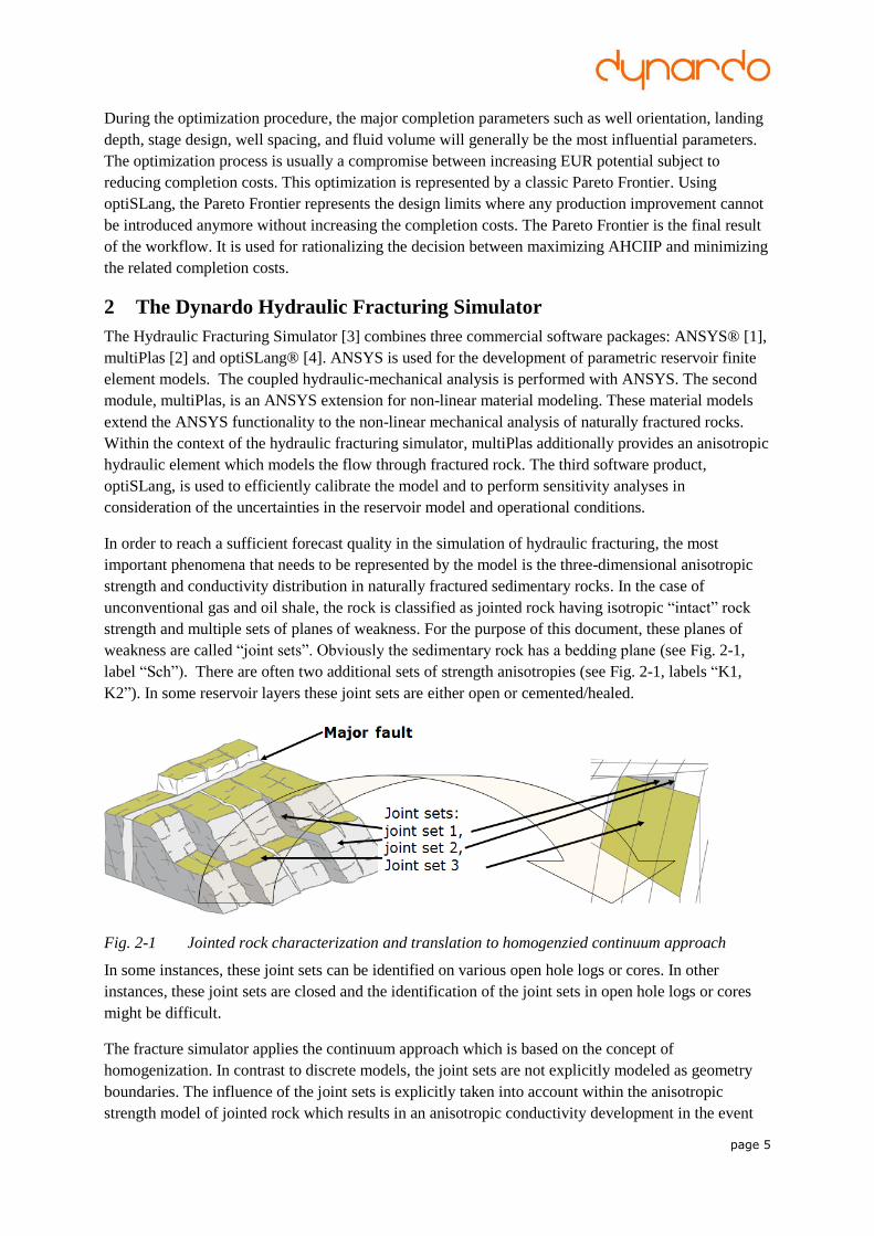
weakness are called “joint sets”. Obviously the sedimentary rock has a bedding plane (see Fig. 2-1,
label “Sch”). There are often two additional sets of strength anisotropies (see Fig. 2-1, labels “K1,
K2”). In some reservoir layers these joint sets are either open or cemented/healed.
Fig. 2-1 Jointed rock characterization and translation to homogenzied continuum approach
In some instances, these joint sets can be identified on various open hole logs or cores. In other
instances, these joint sets are closed and the identification of the joint sets in open hole logs or cores
might be difficult.
The fracture simulator applies the continuum approach which is based on the concept of
homogenization. In contrast to discrete models, the joint sets are not explicitly modeled as geometry
boundaries. The influence of the joint sets is explicitly taken into account within the anisotropic
strength model of jointed rock which results in an anisotropic conductivity development in the event
page 6
of the rock failure represented by the element. Essentially, a joint set dilates opens, and the associated
conductivity increases due to either an oriented tensile or an oriented shear failure. At the conclusion
of the frac job, the net pressure decline may result in the joint set aperture reducing, resulting in a
reduction of the associated conductivity. Both of these effects are taken into account in the simulator.
In the simulation, the tensile and shear failure modes of intact rock and of the individual joint sets are
consistently treated within the framework of multi-surface plasticity [9]. The multi-surface strength
criterion is evaluated at every discretization point in space. If the stress state violates the multi-surface
yield criterion, then plastic strains develop and strength degradation occurs. By introducing “mean
effective” activated joint set frequencies that can be defined for every joint set and for every individual
layer, the homogenized joint openings and the corresponding joint conductivities can be calculated
based on the plastic strains. The individual values can be evaluated and visualized in the post-
processing step. The initial natural frequency of the planes of weakness and the mean effective
activated frequency of stimulated joints will usually vary. As a result, determining the activated
average frequency of joints is an important undertaking in the calibration process.
The homogenization approach can and should be coupled with discrete anisotropies such as major
faults if the dimension of the discrete anisotropies are large compared to the overall modelled 3D
geometry or if discrete effects at major faults are of interest. The fault is modelled as discrete 3D
geometry feature, and an oriented joint set is used to define the shear and tensile strength criteria of the
fault.
2.1 Parametric Reservoir Modeling
The simulation of hydraulic fracturing requires the calibration of important but somewhat uncertain
parameters. The reservoir system, inclusive of the wellbores and the frac stages, should be
parametrically modeled in order to allow for an efficient calibration procedure. The entire process of
model generation (pre-processing), model solution, and model post-processing should ideally be an
automated process. The hydraulic fracturing simulator offers a predefined parametric representation of
the following inputs:
1/ Model geometry: number of wells/stages, stage positions and orientations, number of
perforation clusters per stage, distance between perforations, distance between stages,
well/stage depths, horizontal well orientation, number and depth of all rock units
2/ Finite element mesh: definition of model boundaries, definition of volumes with different
element size (e.g. fine mesh at perforations and coarse mesh at the model boundary), element
size, type of mesh, type of coupling, perforation size
3/ Initial stress field: piece-wise linear distribution (linear inside one layer, but jumps at the
boundary between two layers) of total vertical stress, minimum horizontal effective stress (k0-
values) and maximum horizontal effective stress, direction of minimum horizontal stress
4/ Initial pore pressure field: piece-wise linear distribution of pore pressure (linear inside one
layer, but jumps at the boundary between two layers)
5/ Material properties of all rock layers: linear and nonlinear mechanical material properties
including definition of up to four joint sets, hydraulic material properties
6/ Well treating: slurry rate and bottom hole pressure as a function over time, average proppant
size and proppant pumping, fluid viscosity, perforation conductivities
7/ Coupling parameters: average activated joint set distance, joint set roughness coefficient,
stress dependency of joint conductivity
page 7
8/ Simulation parameters: time stepping, post-processing
The parametric modeling approach is derived from the ANSYS internal programming language
APDL.
Most of the parameters are separately defined for each distinctive rock layer and for each joint set.
Several hundred parameters are generally required for a model run. As part of the parameter
definition/selection processing; the automatic generation of the finite element model, the calculation of
in-situ reservoir conditions, and the well design and the operational conditions are all tested for
consistency before a unique model execution begins. On occasion, a parameter selection is made for a
specific model run that results in an unrealistic (unstable) initial condition. When this occurs, these
unstable models are identified and their run time execution is terminated.
2.2 Coupled Hydraulic-Mechanical Analysis
Hydraulic fracturing is a coupled hydraulic-mechanical problem. In the hydraulic module, the pressure
increases in the fracture initialization location due to the pumping of fluid and low initial rock
permeability. Within the homogenized continuum approach, pressure is treated as “pore pressure”
representing the pressure in the fracture network. In the mechanical part the increase of pressure
modifies the effective stresses acting on the rock. If the pressure is large enough, the jointed rock fails
and fractures start to open. As a result, the rock permeability increases, which directly influences the
pressure distribution in the hydraulic module.
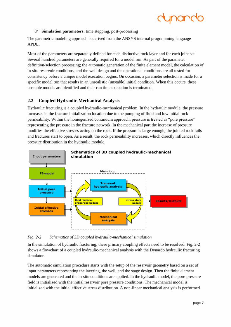
Fig. 2-2 Schematics of 3D coupled hydraulic-mechanical simulation
In the simulation of hydraulic fracturing, these primary coupling effects need to be resolved. Fig. 2-2
shows a flowchart of a coupled hydraulic-mechanical analysis with the Dynardo hydraulic fracturing
simulator.
The automatic simulation procedure starts with the setup of the reservoir geometry based on a set of
input parameters representing the layering, the well, and the stage design. Then the finite element
models are generated and the in-situ conditions are applied. In the hydraulic model, the pore-pressure
field is initialized with the initial reservoir pore pressure conditions. The mechanical model is
initialized with the initial effective stress distribution. A non-linear mechanical analysis is performed
Input parameters
FE-model
Initial pore pressure
Initial effective stresses
Mechanical analysis
Transient hydraulic analysis
Schematics of 3D coupled hydraulic-mechanicalsimulation
Results/Outputs
Main loop
fluid material properties update
stress state update
page 8
to ensure consistency between the mechanical parameters and the initial stress field. The initial
conditions should not result in plastic strains in the model.
After model initialization, the actual simulation cycle for hydraulic fracturing starts. In each cycle, the
hydraulic and the mechanical sub-model are independently solved. The coupling between the models
is realized by an update of material parameters and loading conditions in the corresponding sub-
models. The following couplings are applied:
1/ Stress state update (hydraulic-mechanical coupling): based on the pore-pressure
distribution in the hydraulic model, flow forces are applied in the mechanical analysis.
2/ Fluid material properties update (mechanical-hydraulic coupling): based on the plastic
strain and the stress distribution in the mechanical model, the conductivities are updated in the
hydraulic model. Because of the anisotropic failure of the joint sets, an anisotropic
conductivity tensor is obtained.
The coupling is performed in an explicit way. Consequently, one iteration cycle is performed for every
time step. The time step needs to adequately represent the progress of the fracture growth. The cycle
starts with the transient hydraulic analysis. The pore-pressure field is updated and the corresponding
flow forces are calculated and applied to the mechanical model. The next step is the nonlinear
mechanical analysis which results in a new stress and plastic strain distribution. The resultant update
of the hydraulic conductivities is applied to the hydraulic model in the subsequent time-step.
2.3 Non-Linear Mechanical Analysis
In the mechanical sub-model, a nonlinear static finite element analysis, cf. [10], is performed. The
nonlinearities are caused by failure of the material. In ANSYS, the nonlinear constitutive behavior of
jointed rock is described with the external library multiPlas [2]. By using the ANSYS “usermat” API
for user-defined material models, multiPlas provides nonlinear material models for typical materials in
geomechanical and civil engineering studies.
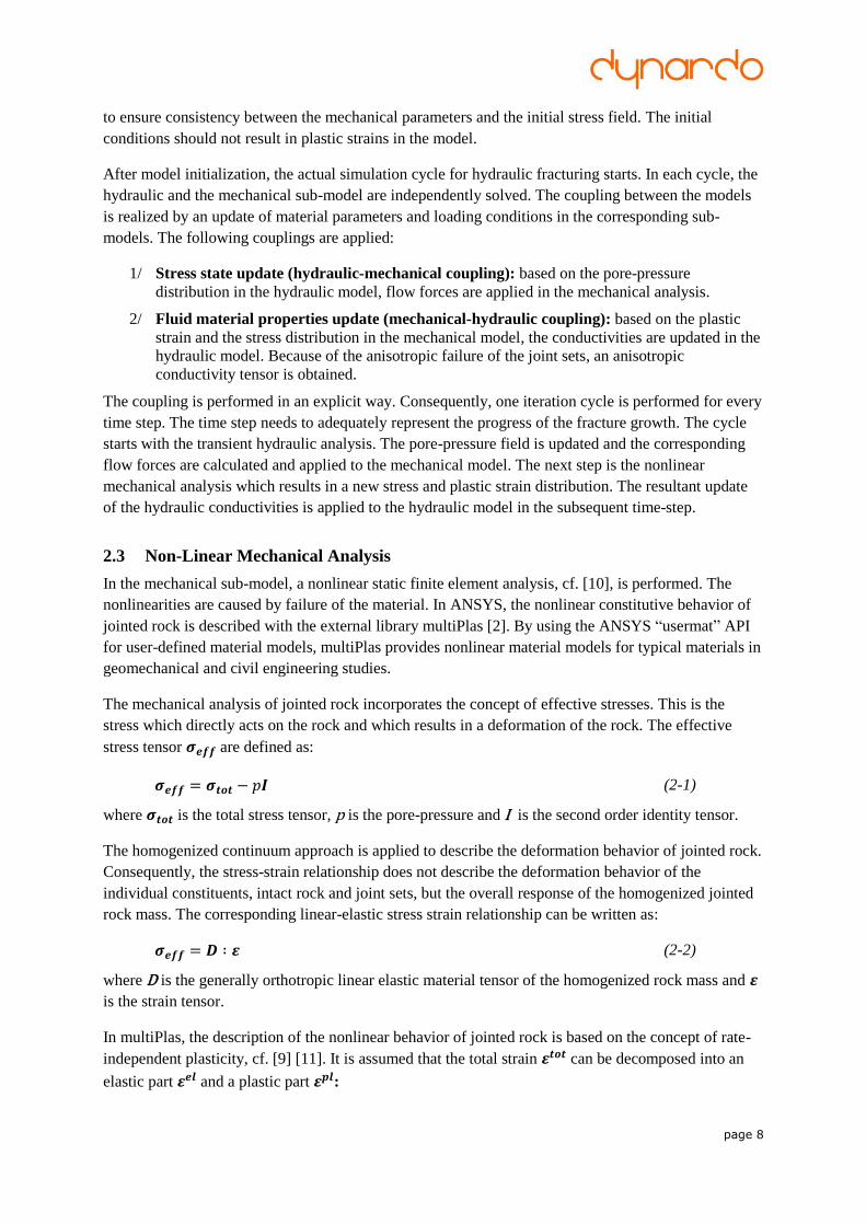
The mechanical analysis of jointed rock incorporates the concept of effective stresses. This is the
stress which directly acts on the rock and which results in a deformation of the rock. The effective
stress tensor 𝝈𝒆𝒇𝒇 are defined as:
𝝈𝒆𝒇𝒇 = 𝝈𝒕𝒐𝒕 − 𝑝𝑰 (2-1)
where 𝝈𝒕𝒐𝒕 is the total stress tensor, p is the pore-pressure and I is the second order identity tensor.
The homogenized continuum approach is applied to describe the deformation behavior of jointed rock.
Consequently, the stress-strain relationship does not describe the deformation behavior of the
individual constituents, intact rock and joint sets, but the overall response of the homogenized jointed
rock mass. The corresponding linear-elastic stress strain relationship can be written as:
𝝈𝒆𝒇𝒇 = 𝑫 ∶ 𝜺 (2-2)
where D is the generally orthotropic linear elastic material tensor of the homogenized rock mass and 𝜺
is the strain tensor.
In multiPlas, the description of the nonlinear behavior of jointed rock is based on the concept of rate-
independent plasticity, cf. [9] [11]. It is assumed that the total strain 𝜺𝒕𝒐𝒕 can be decomposed into an
elastic part 𝜺𝒆𝒍 and a plastic part 𝜺𝒑𝒍:
page 9
𝜺𝒕𝒐𝒕 = 𝜺𝒆𝒍 + 𝜺𝒑𝒍. (2-3)
The stresses are related to the elastic strains by the linear elastic material matrix. Consequently,
Eq. (2-2) can be rewritten as:
𝝈𝒆𝒇𝒇 = 𝑫 ∶ 𝜺𝒆𝒍. (2-4)
The plastic strains develop if a certain strength criterion, conventionally referred to as the yield
condition, is violated. In this context, the boundary of the admissible stress space (elastic domain) is
called yield surface.
The strength of the homogenized jointed rock is defined by the strength of the individual constituents.
As a result, the overall strength criterion is not a smooth surface, but is composed of multiple yield
surfaces. Each yield surface represents a specific failure mode of one of the constituents.
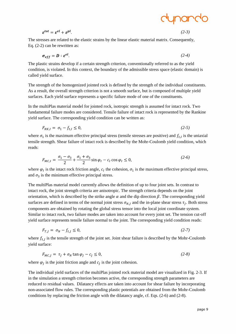
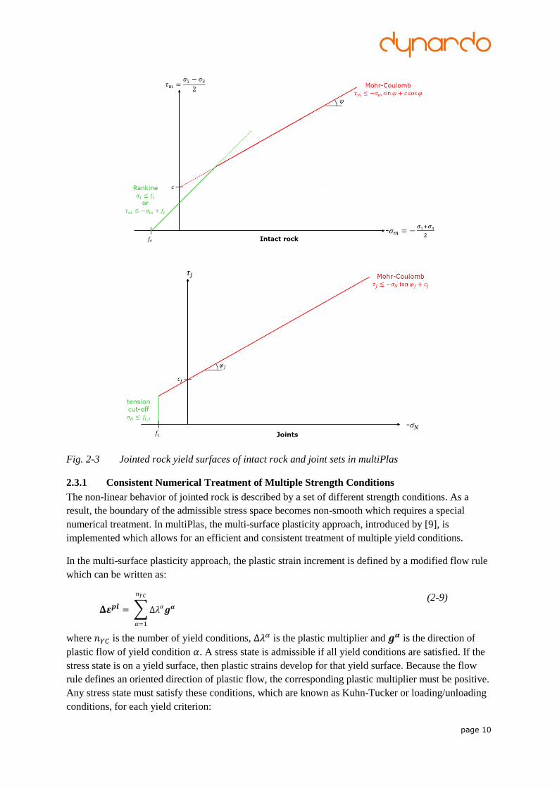
In the multiPlas material model for jointed rock, isotropic strength is assumed for intact rock. Two
fundamental failure modes are considered. Tensile failure of intact rock is represented by the Rankine
yield surface. The corresponding yield condition can be written as:
𝐹𝑅𝐾,𝐼 = 𝜎1 − 𝑓𝑡,𝐼 ≤ 0, (2-5)
where 𝜎1 is the maximum effective principal stress (tensile stresses are positive) and 𝑓𝑡,𝐼 is the uniaxial
tensile strength. Shear failure of intact rock is described by the Mohr-Coulomb yield condition, which
reads:
𝐹𝑀𝐶,𝐼 = 𝜎1 − 𝜎32
+𝜎1 + 𝜎32
sin𝜑𝐼 − 𝑐𝐼 cos𝜑𝐼 ≤ 0, (2-6)
where 𝜑𝐼 is the intact rock friction angle, 𝑐𝐼 the cohesion, 𝜎1 is the maximum effective principal stress,
and 𝜎3 is the minimum effective principal stress.
The multiPlas material model currently allows the definition of up to four joint sets. In contrast to
intact rock, the joint strength criteria are anisotropic. The strength criteria depends on the joint
orientation, which is described by the strike angle 𝛼 and the dip direction 𝛽. The corresponding yield
surfaces are defined in terms of the normal joint stress 𝜎𝑁,𝐽 and the in-plane shear stress 𝜏𝐽. Both stress
components are obtained by rotating the global stress tensor into the local joint coordinate system.
Similar to intact rock, two failure modes are taken into account for every joint set. The tension cut-off
yield surface represents tensile failure normal to the joint. The corresponding yield condition reads:
𝐹𝑇,𝐽 = 𝜎𝑁 − 𝑓𝑡,𝐽 ≤ 0, (2-7)
where 𝑓𝑡,𝐽 is the tensile strength of the joint set. Joint shear failure is described by the Mohr-Coulomb
yield surface:
𝐹𝑀𝐶,𝐽 = 𝜏𝐽 + 𝜎𝑁 tan𝜑𝐽 − 𝑐𝐽 ≤ 0, (2-8)
where 𝜑𝐽 is the joint friction angle and 𝑐𝐽 is the joint cohesion.
The individual yield surfaces of the multiPlas jointed rock material model are visualized in Fig. 2-3. If
in the simulation a strength criterion becomes active, the corresponding strength parameters are
reduced to residual values. Dilatancy effects are taken into account for shear failure by incorporating
non-associated flow rules. The corresponding plastic potentials are obtained from the Mohr-Coulomb
conditions by replacing the friction angle with the dilatancy angle, cf. Eqs. (2-6) and (2-8).
page 10
Fig. 2-3 Jointed rock yield surfaces of intact rock and joint sets in multiPlas
2.3.1 Consistent Numerical Treatment of Multiple Strength Conditions
The non-linear behavior of jointed rock is described by a set of different strength conditions. As a
result, the boundary of the admissible stress space becomes non-smooth which requires a special
numerical treatment. In multiPlas, the multi-surface plasticity approach, introduced by [9], is
implemented which allows for an efficient and consistent treatment of multiple yield conditions.
In the multi-surface plasticity approach, the plastic strain increment is defined by a modified flow rule
which can be written as:
𝚫𝜺𝒑𝒍 = ∑ Δ𝜆𝛼𝒈𝜶
𝑛𝑌𝐶
𝛼=1
(2-9)
where 𝑛𝑌𝐶 is the number of yield conditions, Δ𝜆𝛼 is the plastic multiplier and 𝒈𝜶 is the direction of
plastic flow of yield condition 𝛼. A stress state is admissible if all yield conditions are satisfied. If the
stress state is on a yield surface, then plastic strains develop for that yield surface. Because the flow
rule defines an oriented direction of plastic flow, the corresponding plastic multiplier must be positive.
Any stress state must satisfy these conditions, which are known as Kuhn-Tucker or loading/unloading
conditions, for each yield criterion:
page 11
𝐹𝛼 ≤ 0 𝐹𝛼𝛥𝜆𝛼 = 0 𝛥𝜆𝛼 ≥ 0 𝛼 = 1…𝑛𝑌𝐶. (2-10)
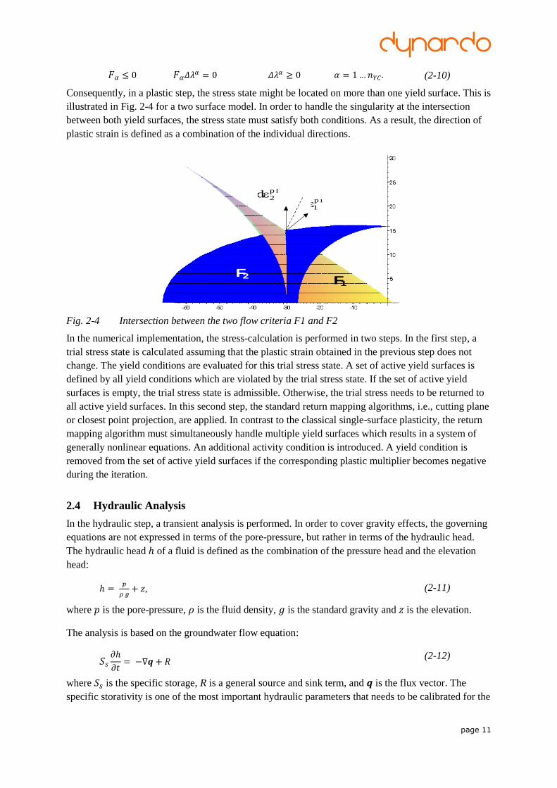
Consequently, in a plastic step, the stress state might be located on more than one yield surface. This is
illustrated in Fig. 2-4 for a two surface model. In order to handle the singularity at the intersection
between both yield surfaces, the stress state must satisfy both conditions. As a result, the direction of
plastic strain is defined as a combination of the individual directions.
p l
1d
p l2d
F1 F2
Fig. 2-4 Intersection between the two flow criteria F1 and F2
In the numerical implementation, the stress-calculation is performed in two steps. In the first step, a
trial stress state is calculated assuming that the plastic strain obtained in the previous step does not
change. The yield conditions are evaluated for this trial stress state. A set of active yield surfaces is
defined by all yield conditions which are violated by the trial stress state. If the set of active yield
surfaces is empty, the trial stress state is admissible. Otherwise, the trial stress needs to be returned to
all active yield surfaces. In this second step, the standard return mapping algorithms, i.e., cutting plane
or closest point projection, are applied. In contrast to the classical single-surface plasticity, the return
mapping algorithm must simultaneously handle multiple yield surfaces which results in a system of
generally nonlinear equations. An additional activity condition is introduced. A yield condition is
removed from the set of active yield surfaces if the corresponding plastic multiplier becomes negative
during the iteration.
2.4 Hydraulic Analysis
In the hydraulic step, a transient analysis is performed. In order to cover gravity effects, the governing
equations are not expressed in terms of the pore-pressure, but rather in terms of the hydraulic head.
The hydraulic head ℎ of a fluid is defined as the combination of the pressure head and the elevation
head:
ℎ = 𝑝
𝜌 𝑔+ 𝑧, (2-11)
where 𝑝 is the pore-pressure, 𝜌 is the fluid density, 𝑔 is the standard gravity and 𝑧 is the elevation.
The analysis is based on the groundwater flow equation:
𝑆𝑠𝜕ℎ
𝜕𝑡= −∇𝒒 + 𝑅
(2-12)
where 𝑆𝑠 is the specific storage, R is a general source and sink term, and 𝒒 is the flux vector. The
specific storativity is one of the most important hydraulic parameters that needs to be calibrated for the
page 12
reservoir. The storativity represents the amount of stored energy in open joints, and is related to the
energy losses due to friction or of leakage during the hydraulic fracturing process.
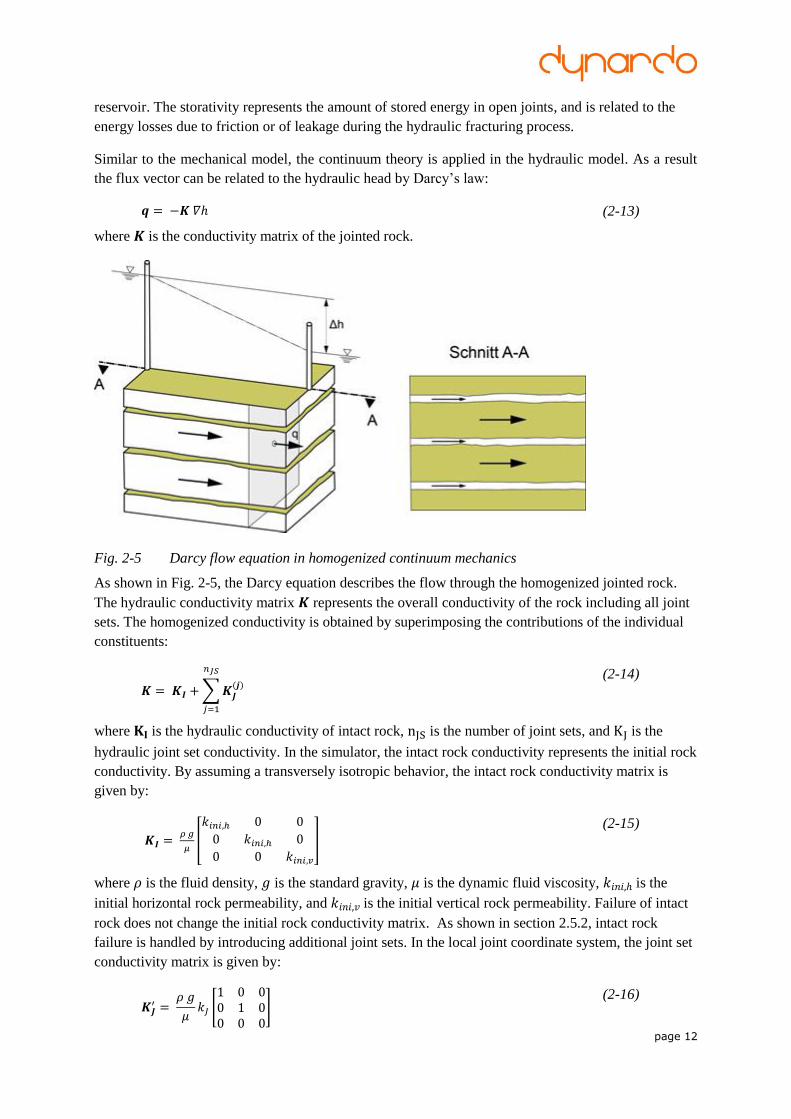
Similar to the mechanical model, the continuum theory is applied in the hydraulic model. As a result
the flux vector can be related to the hydraulic head by Darcy’s law:
𝒒 = −𝑲 𝛻ℎ (2-13)
where 𝑲 is the conductivity matrix of the jointed rock.
Fig. 2-5 Darcy flow equation in homogenized continuum mechanics
As shown in Fig. 2-5, the Darcy equation describes the flow through the homogenized jointed rock.
The hydraulic conductivity matrix 𝑲 represents the overall conductivity of the rock including all joint
sets. The homogenized conductivity is obtained by superimposing the contributions of the individual
constituents:
𝑲 = 𝑲𝑰 +∑𝑲𝑱(𝒋)
𝑛𝐽𝑆
𝑗=1
(2-14)
where 𝐊𝐈 is the hydraulic conductivity of intact rock, nJS is the number of joint sets, and KJ is the
hydraulic joint set conductivity. In the simulator, the intact rock conductivity represents the initial rock
conductivity. By assuming a transversely isotropic behavior, the intact rock conductivity matrix is
given by:
𝑲𝑰 = 𝜌 𝑔
𝜇[
𝑘𝑖𝑛𝑖,ℎ 0 0
0 𝑘𝑖𝑛𝑖,ℎ 0
0 0 𝑘𝑖𝑛𝑖,𝑣
]
(2-15)
where 𝜌 is the fluid density, 𝑔 is the standard gravity, 𝜇 is the dynamic fluid viscosity, 𝑘𝑖𝑛𝑖,ℎ is the
initial horizontal rock permeability, and 𝑘𝑖𝑛𝑖,𝑣 is the initial vertical rock permeability. Failure of intact
rock does not change the initial rock conductivity matrix. As shown in section 2.5.2, intact rock
failure is handled by introducing additional joint sets. In the local joint coordinate system, the joint set
conductivity matrix is given by:
𝑲𝑱′ =
𝜌 𝑔
𝜇𝑘𝐽 [
1 0 00 1 00 0 0
] (2-16)
page 13
where 𝑘𝐽 is the in-plane joint permeability. In the initial state the joint permeability is zero. If a joint
set fails, the joint opens up and the joint permeability increases. This relationship is described in detail
in section 2.5. The global joint conductivity matrix is obtained by rotation of the local matrix:
𝑲𝑱 = 𝑹𝑇𝑲𝑱
′𝑹, (2-17)
where 𝑹 is a matrix describing the rotation from the global into the local joint coordinate system. In
the global coordinate system, the joint conductivity matrix is generally anisotropic. As a result, the
homogenized conductivity matrix 𝑲 becomes anisotropic during the simulation.
By substituting Eq. (2-13) into Eq. (2-12) the transient seepage equation is obtained:
𝑆𝑠𝜕ℎ
𝜕𝑡= −𝛻(𝑲 𝛻ℎ) + 𝑅
(2-18)
This equation is solved by using finite element techniques. Equation (2-18) is analogous to the heat
equation in heat transfer problems. ANSYS heat transfer elements seemingly could solve the problem.
However, because of the anisotropic hydraulic conductivity matrix, Dynardo implemented a new
hydraulic element that more effectively manages the anisotropy.
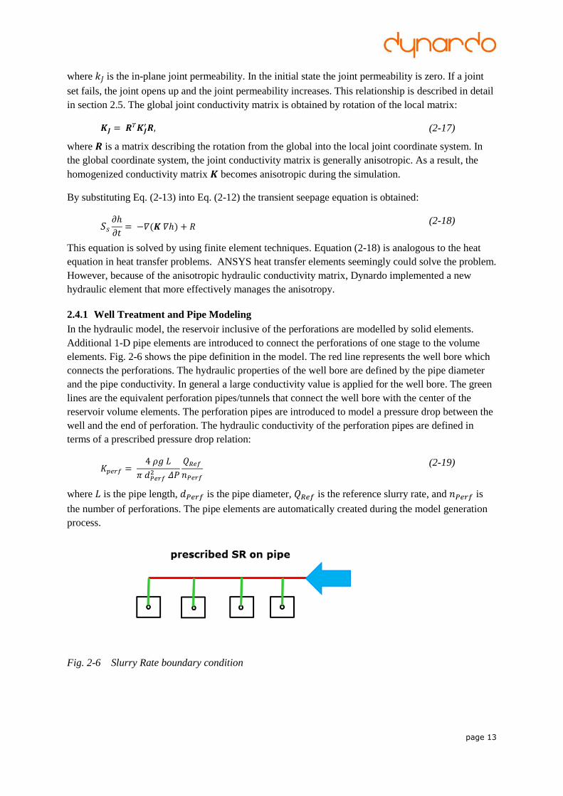
2.4.1 Well Treatment and Pipe Modeling
In the hydraulic model, the reservoir inclusive of the perforations are modelled by solid elements.
Additional 1-D pipe elements are introduced to connect the perforations of one stage to the volume
elements. Fig. 2-6 shows the pipe definition in the model. The red line represents the well bore which
connects the perforations. The hydraulic properties of the well bore are defined by the pipe diameter
and the pipe conductivity. In general a large conductivity value is applied for the well bore. The green
lines are the equivalent perforation pipes/tunnels that connect the well bore with the center of the
reservoir volume elements. The perforation pipes are introduced to model a pressure drop between the
well and the end of perforation. The hydraulic conductivity of the perforation pipes are defined in
terms of a prescribed pressure drop relation:
𝐾𝑝𝑒𝑟𝑓 = 4 𝜌𝑔 𝐿
𝜋 𝑑𝑃𝑒𝑟𝑓2 𝛥𝑃
𝑄𝑅𝑒𝑓
𝑛𝑃𝑒𝑟𝑓
(2-19)
where 𝐿 is the pipe length, 𝑑𝑃𝑒𝑟𝑓 is the pipe diameter, 𝑄𝑅𝑒𝑓 is the reference slurry rate, and 𝑛𝑃𝑒𝑟𝑓 is
the number of perforations. The pipe elements are automatically created during the model generation
process.
Fig. 2-6 Slurry Rate boundary condition
page 14
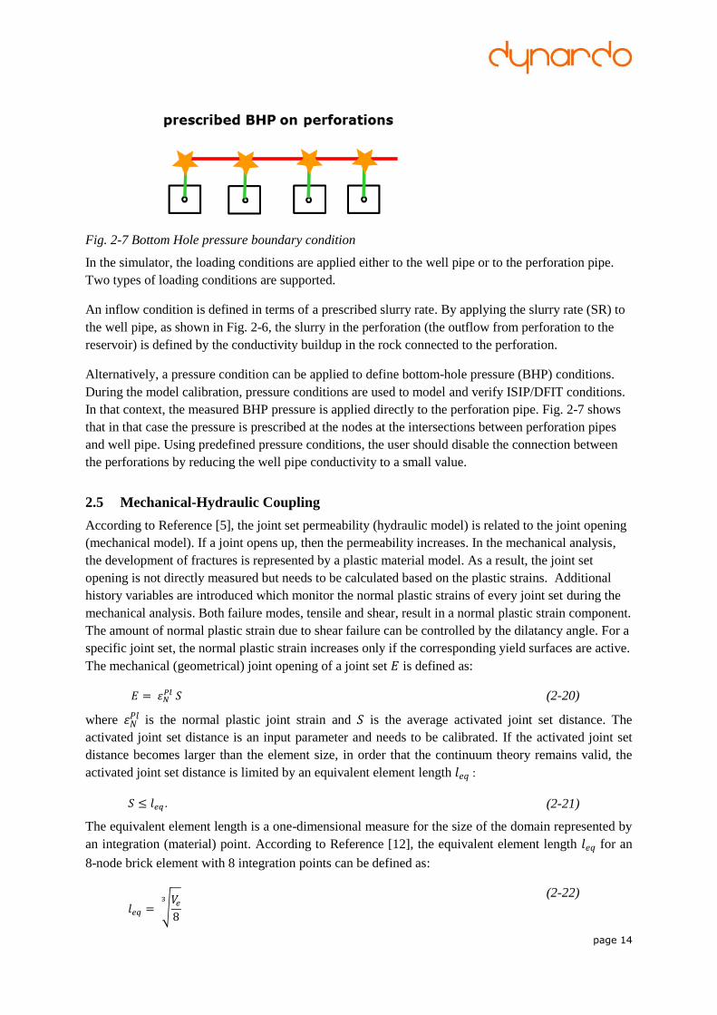
Fig. 2-7 Bottom Hole pressure boundary condition
In the simulator, the loading conditions are applied either to the well pipe or to the perforation pipe.
Two types of loading conditions are supported.
An inflow condition is defined in terms of a prescribed slurry rate. By applying the slurry rate (SR) to
the well pipe, as shown in Fig. 2-6, the slurry in the perforation (the outflow from perforation to the
reservoir) is defined by the conductivity buildup in the rock connected to the perforation.
Alternatively, a pressure condition can be applied to define bottom-hole pressure (BHP) conditions.
During the model calibration, pressure conditions are used to model and verify ISIP/DFIT conditions.
In that context, the measured BHP pressure is applied directly to the perforation pipe. Fig. 2-7 shows
that in that case the pressure is prescribed at the nodes at the intersections between perforation pipes
and well pipe. Using predefined pressure conditions, the user should disable the connection between
the perforations by reducing the well pipe conductivity to a small value.
2.5 Mechanical-Hydraulic Coupling
According to Reference [5], the joint set permeability (hydraulic model) is related to the joint opening
(mechanical model). If a joint opens up, then the permeability increases. In the mechanical analysis,
the development of fractures is represented by a plastic material model. As a result, the joint set
opening is not directly measured but needs to be calculated based on the plastic strains. Additional
history variables are introduced which monitor the normal plastic strains of every joint set during the
mechanical analysis. Both failure modes, tensile and shear, result in a normal plastic strain component.
The amount of normal plastic strain due to shear failure can be controlled by the dilatancy angle. For a
specific joint set, the normal plastic strain increases only if the corresponding yield surfaces are active.
The mechanical (geometrical) joint opening of a joint set 𝐸 is defined as:
𝐸 = 𝜀𝑁𝑃𝑙 𝑆 (2-20)
where 𝜀𝑁𝑃𝑙 is the normal plastic joint strain and 𝑆 is the average activated joint set distance. The
activated joint set distance is an input parameter and needs to be calibrated. If the activated joint set
distance becomes larger than the element size, in order that the continuum theory remains valid, the
activated joint set distance is limited by an equivalent element length 𝑙𝑒𝑞 :
𝑆 ≤ 𝑙𝑒𝑞 . (2-21)
The equivalent element length is a one-dimensional measure for the size of the domain represented by
an integration (material) point. According to Reference [12], the equivalent element length 𝑙𝑒𝑞 for an
8-node brick element with 8 integration points can be defined as:
𝑙𝑒𝑞 = √𝑉𝑒8
3
(2-22)
page 15
where 𝑉𝑒 is the element volume.
In the original derivation of the joint set permeability in Reference [5], a laminar flow between two
smooth planes is assumed. In reality, the joint surface is neither planar nor smooth. Consequently, the
mechanical opening must be related to the effective hydraulic opening of the idealized joint set [13]
[14]. In the simulator, the following relationship is applied:
𝑒 = 𝐸
𝑟𝐸𝑒,
(2-23)
where 𝑒 is the effective hydraulic opening and 𝑟𝐸𝑒 is a prescribed ratio between both opening
measures. In most applications of the simulator, a ratio between 1 and 2 is used initially, and later
adjusted and verified during the calibration process.
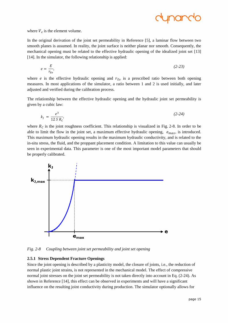
The relationship between the effective hydraulic opening and the hydraulic joint set permeability is
given by a cubic law:
𝑘𝐽 = 𝑒3
12 𝑆 𝑅𝐶,
(2-24)
where 𝑅𝐶 is the joint roughness coefficient. This relationship is visualized in Fig. 2-8. In order to be
able to limit the flow in the joint set, a maximum effective hydraulic opening, 𝑒𝑚𝑎𝑥, is introduced.
This maximum hydraulic opening results in the maximum hydraulic conductivity, and is related to the
in-situ stress, the fluid, and the proppant placement condition. A limitation to this value can usually be
seen in experimental data. This parameter is one of the most important model parameters that should
be properly calibrated.
Fig. 2-8 Coupling between joint set permeability and joint set opening
2.5.1 Stress Dependent Fracture Openings
Since the joint opening is described by a plasticity model, the closure of joints, i.e., the reduction of
normal plastic joint strains, is not represented in the mechanical model. The effect of compressive
normal joint stresses on the joint set permeability is not taken directly into account in Eq. (2-24). As
shown in Reference [14], this effect can be observed in experiments and will have a significant
influence on the resulting joint conductivity during production. The simulator optionally allows for
page 16
this effect to be managed. If the stress dependency is enabled, then the joint set permeability is
calculated as:
𝑘𝐽(𝑒, 𝜎𝑁) = 𝑓(𝜎𝑁)𝑘𝐽0(𝑒), (2-25)
where 𝑘𝐽0 is the stress independent joint set permeability given by Eq. (2-24), 𝑓 is a dimensionless
scaling factor ranging from a minimum value to 1, and 𝜎𝑁 is the normal joint stress. Based on [15] the
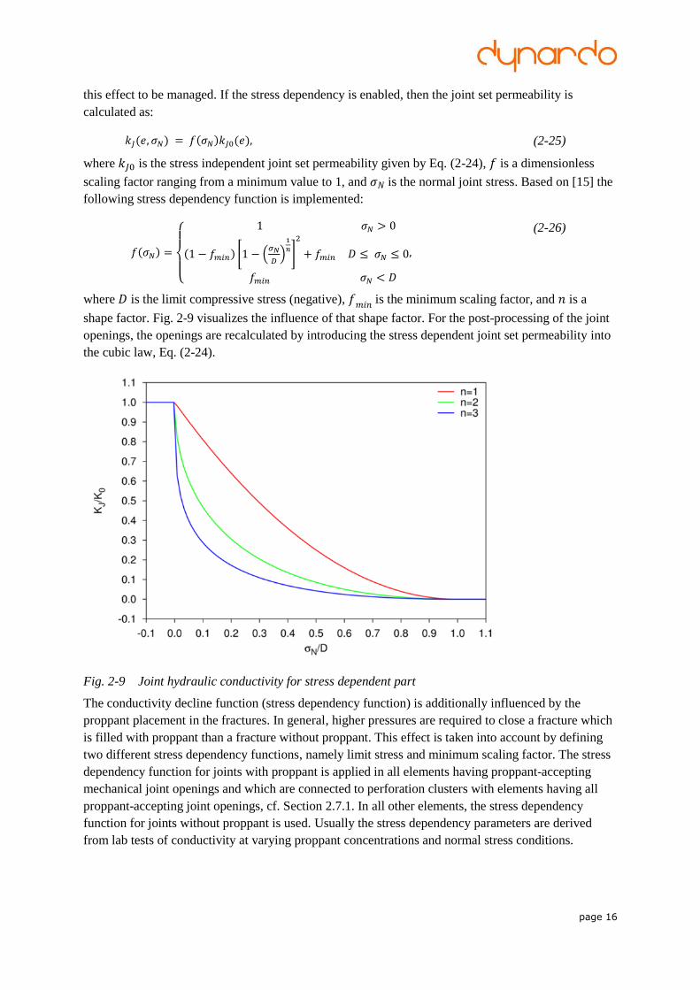
following stress dependency function is implemented:
𝑓(𝜎𝑁) =
{
1 𝜎𝑁 > 0
(1 − 𝑓𝑚𝑖𝑛) [1 − (𝜎𝑁
𝐷)
1
𝑛]
2
+ 𝑓𝑚𝑖𝑛 𝐷 ≤ 𝜎𝑁 ≤ 0
𝑓𝑚𝑖𝑛 𝜎𝑁 < 𝐷
,
(2-26)
where 𝐷 is the limit compressive stress (negative), 𝑓𝑚𝑖𝑛 is the minimum scaling factor, and 𝑛 is a
shape factor. Fig. 2-9 visualizes the influence of that shape factor. For the post-processing of the joint
openings, the openings are recalculated by introducing the stress dependent joint set permeability into
the cubic law, Eq. (2-24).
Fig. 2-9 Joint hydraulic conductivity for stress dependent part
The conductivity decline function (stress dependency function) is additionally influenced by the
proppant placement in the fractures. In general, higher pressures are required to close a fracture which
is filled with proppant than a fracture without proppant. This effect is taken into account by defining
two different stress dependency functions, namely limit stress and minimum scaling factor. The stress
dependency function for joints with proppant is applied in all elements having proppant-accepting
mechanical joint openings and which are connected to perforation clusters with elements having all
proppant-accepting joint openings, cf. Section 2.7.1. In all other elements, the stress dependency
function for joints without proppant is used. Usually the stress dependency parameters are derived
from lab tests of conductivity at varying proppant concentrations and normal stress conditions.
page 17
2.5.2 Influence of Intact Failure on Hydraulic Conductivity Tensor
In addition to joint failure, the intact rock might fail as well, and the hydraulic conductivity of the
jointed rock increases. In order to capture this phenomenon, up to three additional joint sets, one for
tensile failure and two for shear failure, are introduced in case of intact rock failure. These additional
joint sets are introduced if the corresponding intact rock failure criterion is violated for the first time.
In the case of tensile failure where the Rankine yield surface becomes active, the additional joint is
oriented perpendicular to the maximum principal stress direction. In the case of shear failure where the
Mohr-Coulomb yield surface becomes active, the orientation of two additional joint sets coincides
with the orientation of the shear failure planes in that step. After initialization of the additional joint
sets, the orientation is fixed for that element for the duration of the simulation. For these additional
joint sets, the mechanical-hydraulic coupling is performed in the same way as for the pre-defined joint
sets.
From experience in shale reservoirs, the hydraulic conductivity change primarily from intact failure
occurs in fracture barriers, which usually represents reservoir layers without vertical joint sets.
2.6 Hydraulic-Mechanical Coupling
Fluid flow in joints results in normal forces and shear forces at the joint walls [5]. The flow forces are
related to the pore-pressure gradient. In the global orientation, the flow force vector 𝑱𝒇𝒇 acting on the
element volume (body force) can be written as:
𝑱𝒇𝒇 = 𝜌 𝑔 𝑰 𝑰𝑇 = [
𝜕ℎ
𝜕𝑥
𝜕ℎ
𝜕𝑦
𝜕ℎ
𝜕𝑧]
(2-27)
where 𝜌 is the fluid density, 𝑔 is the standard gravity, and 𝑰 is the gradient of the hydraulic head. The
corresponding nodal force vector is obtained by integration of the flow force vector over the element
volume. The individual nodal contributions are assembled and transferred to the mechanical model.
Because of the incremental solution procedure, only the variation in the flow forces is added to the
nodal forces in the mechanical model at every time step.
2.7 Post Processing
In addition to the traditional ANSYS post-processing functionality, e.g., stress plots, the simulator
provides additional hydraulic fracturing specific outputs. These additional post-processing features are
provided as parameterized APDL macros. In order to reduce the amount of data which is produced
during the simulation and in order to reduce the total simulation time, the frequency of post-processing
steps is also parameterized. The additional post-processing includes:
bottom hole pressure and slurry rate over time (per perforation and per stage)
fluid and fracture volume balance, e.g. fluid inflow and created joint volumes over time
plots of joint set openings, joint set conductivities
pore-pressure plots
plots of the stimulated rock including microseismic events (all plastic elements, connected
water-accepting plastic elements and connected proppant-accepting plastic elements) and the
corresponding stimulated rock volume over time
plastic activity over time
connected drainage volume
fracture extension compared to microseismic events
In addition to this predefined post-processing macros, all results can be exported into ASCII files.
page 18
2.7.1 Calculation of Connected Water and Proppant-Accepting Volume
Based on the mechanical joint openings, elements are identified as water-accepting or as proppant-
accepting. An element becomes water-accepting if the mechanical opening of at least one joint set
exceeds a predefined threshold. This threshold is parameterized. Usually a threshold of 0.1 mm is
applied. A proppant-accepting element is identified if the mechanical opening of at least one joint set
exceeds a multiple of the average proppant size. The factor and the average proppant size are also
parameters of the model. In most of the reservoirs, a threshold of 3 times the average proppant size is
applied.
In addition to the water and proppant-accepting elements, the corresponding connected sets of water
and proppant-accepting elements are identified. An element is part of the set of connected water-
accepting elements if the fluid can flow from any perforation into that element only by flowing
through the other elements in that set. The sets of connected water and of connected proppant-
accepting elements are continuously updated during the simulation. At the beginning of the
simulation, the perforation elements are added to the connected sets. After every mechanical step, the
water and proppant-accepting elements are identified. Based on the connected sets from the previous
step, the neighbouring water or proppant-accepting elements are selected and added to the
corresponding connected set. Two elements are neighbours if they are connected by at least one node.
This selection algorithm is continued until no new neighbour elements are found. The sets of
connected elements are history dependent.
For connected proppant-accepting volumes, the possibility of successful proppant placement is
presumed. If proppant is placed in the fractures, it has an influence on the conductivity decline
function, cf. Section 2.5.1. The stress dependency function for joints with proppant is only used for
elements which are part of the set of connected proppant-accepting volume. Otherwise the stress
dependency function for joints without proppant is applied even if the opening is larger than the
proppant-accepting opening threshold.
2.7.2 Calculation Connected Drainage Volume
Based on the set of connected proppant-accepting elements, the drainage volume can be calculated.
The drainage volume is defined by all elements which can be drained during the production time of
the well from the set of connected proppant-accepting elements. The corresponding elements are
identified by selecting, from the set of “connected proppant-accepting elements,” all elements which
satisfy the following criteria:
The element is in the same element layer of the layered reservoir as the connected proppant-
accepting element. This is based on the assumption that only the “horizontal” initial
permeability of unstimulated rock provides a mechanism for flow through unstimulated rock,
this horizontal permeability being several orders of magnitude larger than the effective vertical
permeability.
The distance between the element center and the center of the proppant-accepting element is
less than the drainage radius.
page 19
3 Application to North American Reservoir
3.1 Milestones and Goals
After several years of field development, the standard completion practices in the Reservoir were
investigated for the potential to improve hydrocarbon production. The workflow was applied. The
hydraulic fracturing simulator was calibrated to a well with a suitable set of whole core and log data,
as well as quality microseismic. After calibration, a sensitivity analysis to possible variations of
operational conditions was performed, and Meta-Models of the Optimal Prognosis (MOP) was
derived. These Meta-Models were derived from multiple simulation results. They represented a
verified correlation between all of the inputs to the model and the simulation results. The forecast
quality of the MOP’s was verified during the calibration phase and confirmed with offset well
production performance. The Meta-Models were then used in a fully predictive mode to optimize the
completion design subject to economic considerations (e.g., maximum VSRV, AHCIIP, hydrocarbon
production, costs).
3.2 Modeling of the Calibration Well and the Calibration Stages
One well out of a pad of four wells was chosen as the calibration well. It was the first well on the pad
that was completed. When considering the effects of fracturing induced inter-stage stress shadowing,
the modeling of three successive stages appeared adequate.
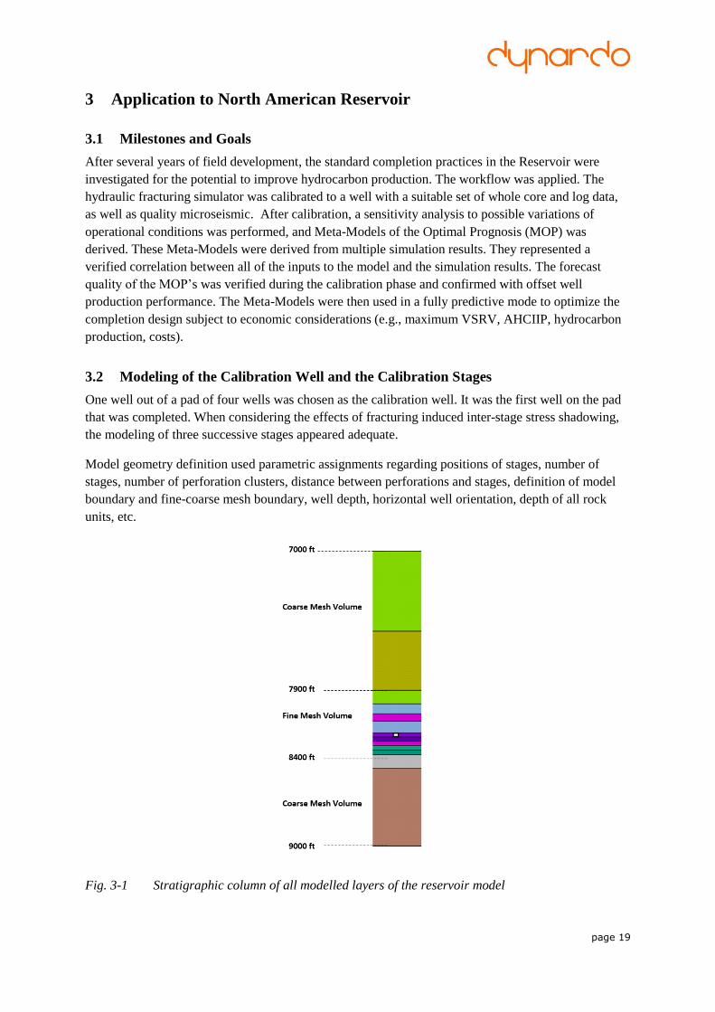
Model geometry definition used parametric assignments regarding positions of stages, number of
stages, number of perforation clusters, distance between perforations and stages, definition of model
boundary and fine-coarse mesh boundary, well depth, horizontal well orientation, depth of all rock
units, etc.
Fig. 3-1 Stratigraphic column of all modelled layers of the reservoir model
page 20
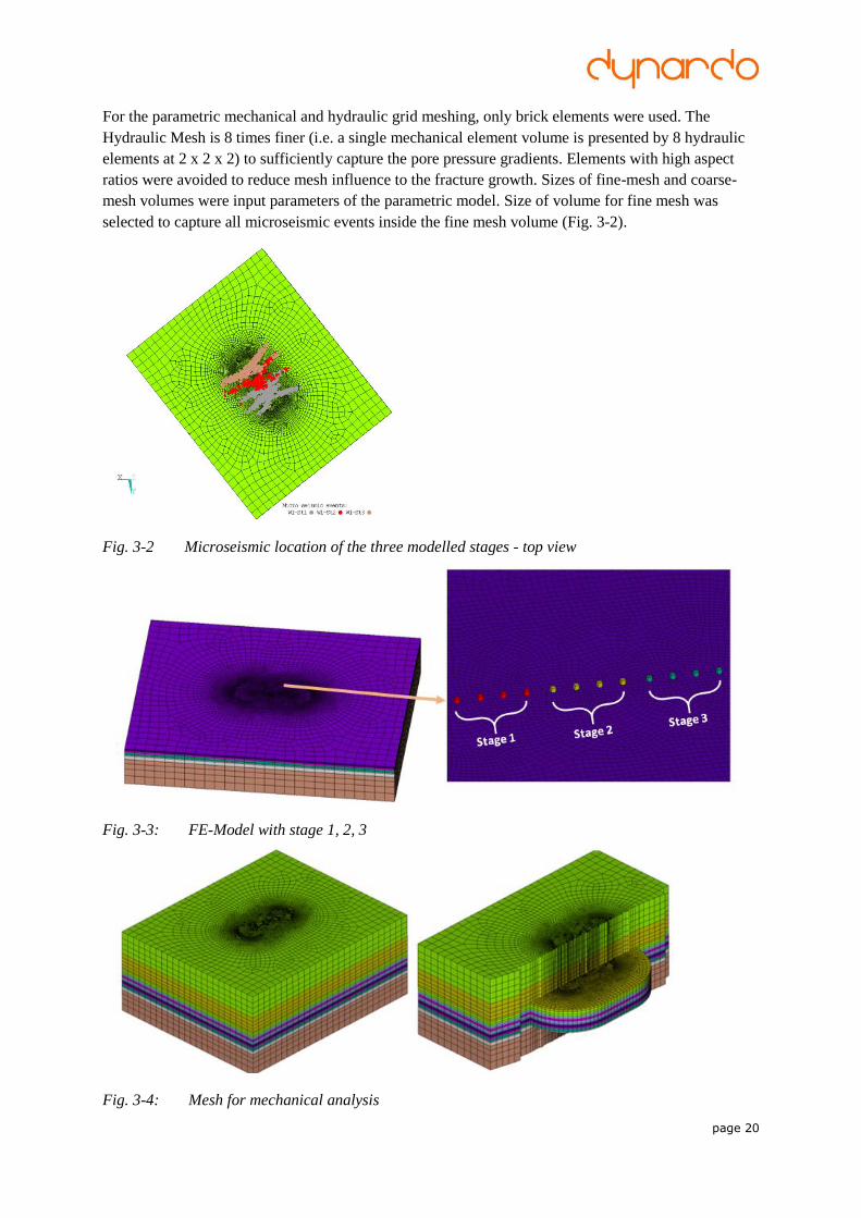
For the parametric mechanical and hydraulic grid meshing, only brick elements were used. The
Hydraulic Mesh is 8 times finer (i.e. a single mechanical element volume is presented by 8 hydraulic
elements at 2 x 2 x 2) to sufficiently capture the pore pressure gradients. Elements with high aspect
ratios were avoided to reduce mesh influence to the fracture growth. Sizes of fine-mesh and coarse-
mesh volumes were input parameters of the parametric model. Size of volume for fine mesh was
selected to capture all microseismic events inside the fine mesh volume (Fig. 3-2).
Fig. 3-2 Microseismic location of the three modelled stages - top view
Fig. 3-3: FE-Model with stage 1, 2, 3
Fig. 3-4: Mesh for mechanical analysis
page 21
3.3 Definition of Reservoir Parameters
Initial elastic properties of layers and UCS values were taken from log and core data analysis. Initial
strength properties of intact rock were derived from UCS values. Intact rock tensile strength was
initially assumed to be 10% of UCS for all layers. Defining the friction angle of intact rock initially to
45°, cohesion values were then calculated.
Based on micro-seismic data, core, and log data interpretation, the expected fracture barriers were
located in two different layer. The barriers were initially modelled without initial vertical joint sets.
Model boundary layers where no fracture penetration was seen in the microseismic surveys were
modelled with elastic material properties. Initial joint set strength parameters were derived from
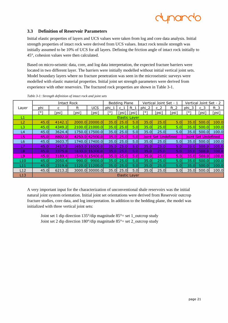
experience with other reservoirs. The fractured rock properties are shown in Table 3-1.
Table 3-1: Strength definition of intact rock and joint sets
Layer Intact Rock Bedding Plane Vertical Joint Set - 1 Vertical Joint Set - 2
phi c ft UCS phi_1 c_1 ft_1 phi_2 c_2 ft_2 phi_3 c_3 ft_3 [°] [psi] [psi] [psi] [°] [psi] [psi] [°] [psi] [psi] [°] [psi] [psi]
L1 Elastic Layer L2 45.0 4142.1 2000.0 20000.0 35.0 25.0 5.0 35.0 25.0 5.0 35.0 500.0 100.0 L3 45.0 4349.2 2100.0 21000.0 35.0 25.0 5.0 35.0 25.0 5.0 35.0 500.0 100.0 L4 45.0 3624.4 1750.0 17500.0 35.0 25.0 5.0 35.0 25.0 5.0 35.0 500.0 100.0 L5 45.0 8802.0 4250.0 42500.0 35.0 25.0 5.0 Joint Set Undefined Joint Set Undefined L6 45.0 3603.7 1740.0 17400.0 35.0 25.0 5.0 35.0 25.0 5.0 35.0 500.0 100.0 L7 45.0 3417.3 1650.0 16500.0 35.0 25.0 5.0 35.0 25.0 5.0 35.0 500.0 100.0 L8 45.0 3375.8 1630.0 16300.0 35.0 25.0 5.0 35.0 25.0 5.0 35.0 500.0 100.0 L9 45.0 3189.4 1540.0 15400.0 35.0 25.0 5.0 35.0 25.0 5.0 35.0 500.0 100.0 L10 45.0 2050.4 990.0 9900.0 35.0 25.0 5.0 35.0 25.0 5.0 35.0 500.0 100.0 L11 45.0 2319.6 1120.0 11200.0 35.0 25.0 5.0 35.0 25.0 5.0 35.0 500.0 100.0 L12 45.0 6213.2 3000.0 30000.0 35.0 25.0 5.0 35.0 25.0 5.0 35.0 500.0 100.0 L13 Elastic Layer
A very important input for the characterization of unconventional shale reservoirs was the initial
natural joint system orientation. Initial joint set orientations were derived from Reservoir outcrop
fracture studies, core data, and log interpretation. In addition to the bedding plane, the model was
initialized with three vertical joint sets:
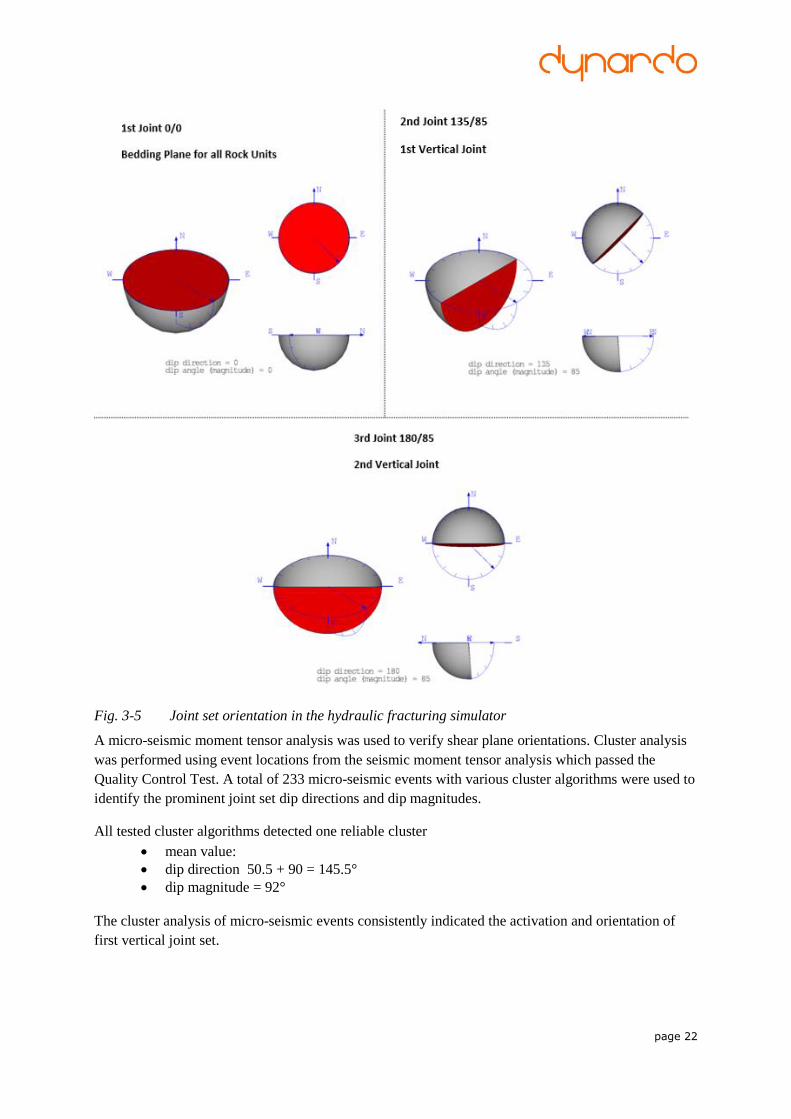
Joint set 1 dip direction 135°/dip magnitude 85°= set 1_outcrop study
Joint set 2 dip direction 180°/dip magnitude 85°= set 2_outcrop study
page 22
Fig. 3-5 Joint set orientation in the hydraulic fracturing simulator
A micro-seismic moment tensor analysis was used to verify shear plane orientations. Cluster analysis
was performed using event locations from the seismic moment tensor analysis which passed the
Quality Control Test. A total of 233 micro-seismic events with various cluster algorithms were used to
identify the prominent joint set dip directions and dip magnitudes.
All tested cluster algorithms detected one reliable cluster
mean value:
dip direction 50.5 + 90 = 145.5°
dip magnitude = 92°
The cluster analysis of micro-seismic events consistently indicated the activation and orientation of
first vertical joint set.
page 23
3.4 Definition of Hydraulic Parameters
The fluid density and fluid viscosity were usually defined as an average fluid parameter for the entire
stage. Because varying amount of gel additives were used during the frac jobs, an average effective
fluid viscosity was calculated and applied to the model. This viscosity term affected the fracture
system; not the wellbore. The projected bottom hole pressure during the frac job was applied as a
boundary condition in the model, and this was provided by the service company performing the frac
job.
Based on measurements used for the definition of the stress dependency of the fracture conductivity
function, a limit stress without proppant placed for all joints (D1) of 4000 psi was defined, and a limit
stress with proppant placed for all joints (D2) of 12000 psi. The minimum hydraulic conductivity
scaling factor without proppant placed for all joints was 0.001 inches. The minimum hydraulic
conductivity scaling factor with proppant placed was 0.01 inches for all joints. The shape factor of the
stress dependent function was defined at 2.0 for all joints. These terms represented the deterioration of
fracture conductivity with increasing normal stress subject to the defined limits.
Specific storativity was defined to be either constant or varying with time. From experience in other
fields, a specific storativity value was defined, and then calibrated with the measured bottom hole
pressure response of the frac job.
Hydraulic properties of the well bore conductivity were defined at 150 (ft/s), having a well bore
diameter of 4.67 inch. The hydraulic properties of the perforation tunnels with a pressure drop of 300
psi at average slurry rate of 50 bpm resulted in a perforation tunnel conductivity of Kperf = 0.31
(ft/sec).
Based on measurement data, anisotropic initial horizontal and vertical permeability values were used.
To estimate the effective drainage radius, the following empirical formula was applied:
𝑅 [𝑓𝑡] = 11.5√𝑘𝑖𝑛𝑖,ℎ [𝑛𝐷], (3-1)
where 𝑘𝑖𝑛𝑖,ℎ is the initial horizontal permeability in the element (in the layer).
The drainage reservoir volume was calculated assuming an initial horizontal permeability of 10 nano
Darcy for upper pay zone layers and 30 nano Darcy for lower pay zone layers. As a result drainage
radii of 36 ft for the upper layers and of 73 ft for the lower layers was applied.
3.5 Initial in-situ Pore Pressure and Effective Stress Conditions
Initial pore pressure is defined for all layers using an initial pore pressure gradient of 0.74 psi/ft. Initial
in-situ stress field is defined as effective stress for every layer of the reservoir by using a vertical total
stress gradient (overburden gradient) of 1.08 psi/ft and conventional relationship between effective
vertical stress SZ and effective minimum horizontal stress SH,min (k0-values) as well as effective
maximum horizontal stress SHmax.
Values for k0 for every layer vary between 0.4 and 0.8. The SHmax is defined to be an increment of 30%
of the difference between SZ and SH,min relative to SH,min. The direction of maximum horizontal stress
direction was defined as being essentially perpendicular to the well direction.
page 24
4 Calibration
Because of the numerous uncertainties in reservoir conditions, calibration of the simulator to the frac
job report and to microseismic events was important. A step wise calibration process was used which
checked the plausibility and balance of simulator inputs to:
- ensure that in-situ strength, stress, and pore pressure values do not result in unrealistic plastic
deformation
- ensure that the model starts and stops fracturing at DFIT/ISIP conditions
- ensure that the model represents fracture growth in time and space by matching the pressure
and the pumping rate histories
- ensure that the volume balance between pumped fluid and created fracture volume results in
the expected fluid efficiency
- ensure a reasonable match to microseismic measurement, that the model shows plausible
fracture direction, extension, and fracture barriers.
During these plausibility controls and calibration steps, significant input parameters are fully checked
and calibrated before starting a full systematic sensitivity analysis. The objective is to establish a set of
parameters with a defined variation space that fulfills all verifications and gives the best possible fit
respective of all available data and their associated uncertainties.
4.1 Calibrating of Fracture Start and Stop Conditions
After verifying that the in-situ initialization of the anisotropic stress field and the pore pressure
conditions of the reservoir rock did not violate the material strength definition, the pressure levels
where fractures start and stop were verified. Diagnostic Fracture Injection Test (DFIT) analysis and
the pressure levels from ISIP (initial shut in pressure) define where fracture initiation and
representative fracture extension pressures occur. There was also an estimation of the uncertainty of
the data, with estimated minimal, mean, and maximal DFIT/ISIP conditions. After initializing a model
with bottom-hole pressure to DFIT/ISIP pressure conditions, a model check was made to view the
simulation results of the expected start and stop of fracture growth.
Typical adjustments during calibration to DFIT/ISIP conditions were:
- Adjustments of pore pressure and in-situ stress conditions at and around the perforation layer
- Adjustments of strength definition of the fracture mode (joint set) where the fracture starts and
stops.
4.2 Calibration of Bottom Hole Pressure Response
After verifying the pressure levels associated with fracture starting and stopping, a verification of
fracture growth rate was made. When pumping a frac stage, the resultant Bottom Hole Pressure (BHP)
signal coupled with rate represents the speed at which the fracture network and fracture conductivity
was created subject to the defined stress and strength conditions in the reservoir. The principal
properties calibrated in this step included:
the activated mean average joint distances in the different layers for intact rock failure and
natural joints activation
maximum effective hydraulic opening in the joint network
strength properties of the reservoir rock outside perforation layer
page 25
the overall loss in energy due to friction, leak off, turbulent flow or other dissipate mechanism
that was summarized into the specific storativity value of the Darcy flow equation.
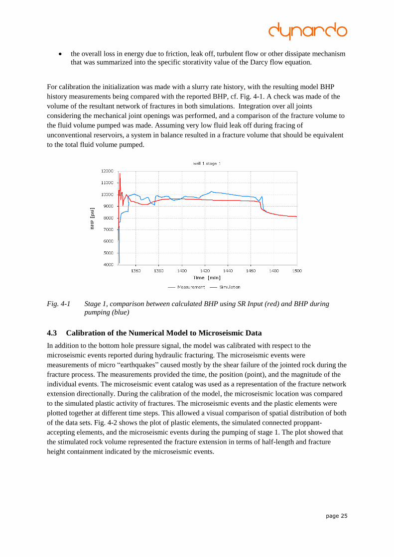
For calibration the initialization was made with a slurry rate history, with the resulting model BHP
history measurements being compared with the reported BHP, cf. Fig. 4-1. A check was made of the
volume of the resultant network of fractures in both simulations. Integration over all joints
considering the mechanical joint openings was performed, and a comparison of the fracture volume to
the fluid volume pumped was made. Assuming very low fluid leak off during fracing of
unconventional reservoirs, a system in balance resulted in a fracture volume that should be equivalent
to the total fluid volume pumped.
Fig. 4-1 Stage 1, comparison between calculated BHP using SR Input (red) and BHP during
pumping (blue)
4.3 Calibration of the Numerical Model to Microseismic Data
In addition to the bottom hole pressure signal, the model was calibrated with respect to the
microseismic events reported during hydraulic fracturing. The microseismic events were
measurements of micro “earthquakes” caused mostly by the shear failure of the jointed rock during the
fracture process. The measurements provided the time, the position (point), and the magnitude of the
individual events. The microseismic event catalog was used as a representation of the fracture network
extension directionally. During the calibration of the model, the microseismic location was compared
to the simulated plastic activity of fractures. The microseismic events and the plastic elements were
plotted together at different time steps. This allowed a visual comparison of spatial distribution of both
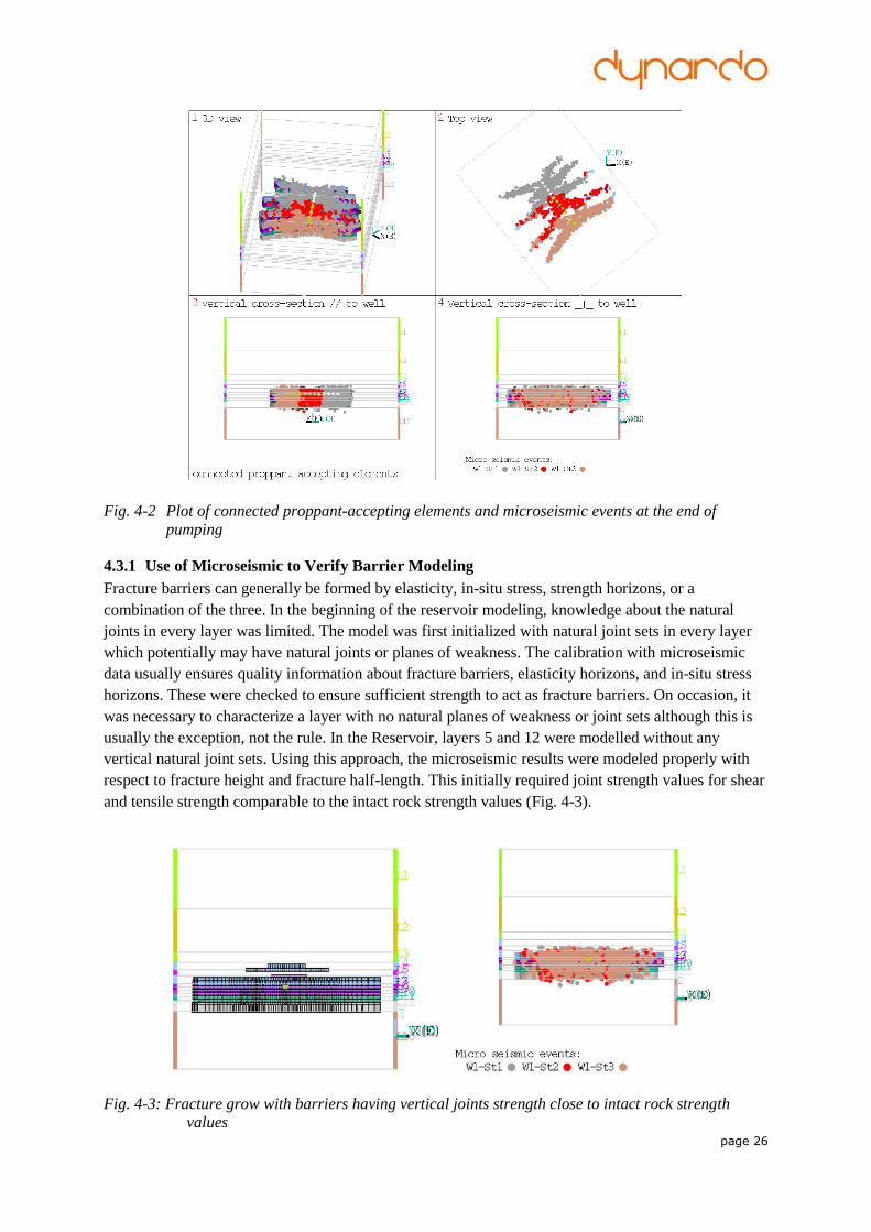
of the data sets. Fig. 4-2 shows the plot of plastic elements, the simulated connected proppant-
accepting elements, and the microseismic events during the pumping of stage 1. The plot showed that
the stimulated rock volume represented the fracture extension in terms of half-length and fracture
height containment indicated by the microseismic events.
page 26
Fig. 4-2 Plot of connected proppant-accepting elements and microseismic events at the end of
pumping
4.3.1 Use of Microseismic to Verify Barrier Modeling
Fracture barriers can generally be formed by elasticity, in-situ stress, strength horizons, or a
combination of the three. In the beginning of the reservoir modeling, knowledge about the natural
joints in every layer was limited. The model was first initialized with natural joint sets in every layer
which potentially may have natural joints or planes of weakness. The calibration with microseismic
data usually ensures quality information about fracture barriers, elasticity horizons, and in-situ stress
horizons. These were checked to ensure sufficient strength to act as fracture barriers. On occasion, it
was necessary to characterize a layer with no natural planes of weakness or joint sets although this is
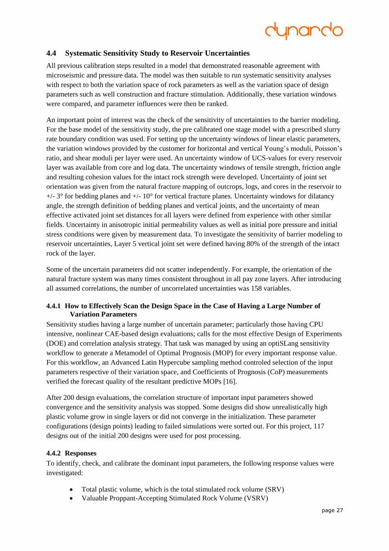
usually the exception, not the rule. In the Reservoir, layers 5 and 12 were modelled without any
vertical natural joint sets. Using this approach, the microseismic results were modeled properly with
respect to fracture height and fracture half-length. This initially required joint strength values for shear
and tensile strength comparable to the intact rock strength values (Fig. 4-3).
Fig. 4-3: Fracture grow with barriers having vertical joints strength close to intact rock strength
values
page 27
4.4 Systematic Sensitivity Study to Reservoir Uncertainties
All previous calibration steps resulted in a model that demonstrated reasonable agreement with
microseismic and pressure data. The model was then suitable to run systematic sensitivity analyses
with respect to both the variation space of rock parameters as well as the variation space of design
parameters such as well construction and fracture stimulation. Additionally, these variation windows
were compared, and parameter influences were then be ranked.
An important point of interest was the check of the sensitivity of uncertainties to the barrier modeling.
For the base model of the sensitivity study, the pre calibrated one stage model with a prescribed slurry
rate boundary condition was used. For setting up the uncertainty windows of linear elastic parameters,
the variation windows provided by the customer for horizontal and vertical Young’s moduli, Poisson’s
ratio, and shear moduli per layer were used. An uncertainty window of UCS-values for every reservoir
layer was available from core and log data. The uncertainty windows of tensile strength, friction angle
and resulting cohesion values for the intact rock strength were developed. Uncertainty of joint set
orientation was given from the natural fracture mapping of outcrops, logs, and cores in the reservoir to
+/- 3° for bedding planes and +/- 10° for vertical fracture planes. Uncertainty windows for dilatancy
angle, the strength definition of bedding planes and vertical joints, and the uncertainty of mean
effective activated joint set distances for all layers were defined from experience with other similar
fields. Uncertainty in anisotropic initial permeability values as well as initial pore pressure and initial
stress conditions were given by measurement data. To investigate the sensitivity of barrier modeling to
reservoir uncertainties, Layer 5 vertical joint set were defined having 80% of the strength of the intact
rock of the layer.
Some of the uncertain parameters did not scatter independently. For example, the orientation of the
natural fracture system was many times consistent throughout in all pay zone layers. After introducing
all assumed correlations, the number of uncorrelated uncertainties was 158 variables.
4.4.1 How to Effectively Scan the Design Space in the Case of Having a Large Number of
Variation Parameters
Sensitivity studies having a large number of uncertain parameter; particularly those having CPU
intensive, nonlinear CAE-based design evaluations; calls for the most effective Design of Experiments
(DOE) and correlation analysis strategy. That task was managed by using an optiSLang sensitivity
workflow to generate a Metamodel of Optimal Prognosis (MOP) for every important response value.
For this workflow, an Advanced Latin Hypercube sampling method controled selection of the input
parameters respective of their variation space, and Coefficients of Prognosis (CoP) measurements
verified the forecast quality of the resultant predictive MOPs [16].
After 200 design evaluations, the correlation structure of important input parameters showed
convergence and the sensitivity analysis was stopped. Some designs did show unrealistically high
plastic volume grow in single layers or did not converge in the initialization. These parameter
configurations (design points) leading to failed simulations were sorted out. For this project, 117
designs out of the initial 200 designs were used for post processing.
4.4.2 Responses
To identify, check, and calibrate the dominant input parameters, the following response values were
investigated:
Total plastic volume, which is the total stimulated rock volume (SRV)
Valuable Proppant-Accepting Stimulated Rock Volume (VSRV)
page 28
Sum of element volumes having plastic activity at barrier layer (Layer 5)
Fracture height, half-length, and fracture density function and the related shape error
4.4.3 Principal Results of the Sensitivity Analysis
After achieving a reasonable match to the Bottom Hole Pressure function, the main objective of the
continued analysis was to improve the fit to the microseismic event catalog.
An investigation into the simulation results then focused on the relative penetration of the soft barrier
layer 5. Out of the 117 viable design simulations, only 15 designs clearly matched the microseismic
event observations with regard to this apparent frac barrier. This indicated that the strength values of
layer 5 barrier (joint sets have 80% of intact rock strength) represented a much too small strength. As
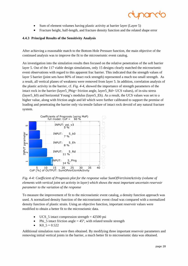
a result, all vertical planes of weakness were removed from layer 5. In addition, correlation analysis of
the plastic activity in the barrier, cf. Fig. 4-4, showed the importance of strength parameters of the
intact rock in the barrier (layer5_Phig= friction angle, layer5_Rd= UCS values), of in-situ stress
(layer5_k0) and horizontal Young’s modulus (layer5_Eh). As a result, the UCS values was set to a
higher value, along with friction angle and k0 which were further calibrated to support the premise of
loading and penetrating the barrier only via tensile failure of intact rock devoid of any natural fracture
system.
Fig. 4-4: Coefficient of Prognosis plot for the response value SumOfVertJointActivity (volume of
elements with vertical joint set activity in layer) which shows the most important uncertain reservoir
parameter to the variation of the response
To measure the improvement of fit to the microseismic event catalog, a density function approach was
used. A normalized density function of the microseismic event cloud was compared with a normalized
density function of plastic strain. Using an objective function, important reservoir values were
modified to obtain a better fit to the microseismic data.
UCS_5 intact compression strength = 42500 psi
Phi_5 intact friction angle = 45°, with related tensile strength
K0_5 = 0.522
Additional simulation runs were then obtained. By modifying three important reservoir parameters and
removing initial vertical joints in the barrier, a much better fit to microseismic data was obtained.

page 29
5 Sensitivity to Operational Conditions
Sensitivity analyses relative to the operational parameters was then performed in order to establish the
cost/benefit relationship related to well drilling and completion practices. EUR improvements were
derived from increases in the valuable stimulated rock volume (VSRV) and the resulting increase in
accessible gas initially in place (AHCIIP).
5.1 Reference design for sensitivity analysis
As reference design, the calibrated model of hydraulic fracturing was used. In order to forecast
variation of valuable stimulated rock volume and drainage volumes, multiple stage simulations were
required. The initial simulation stage did not see stress shadowing, but the effect of stress shadowing
is an important consideration for the optimization of the stage design. A multistage simulation exercise
is required to better capture the stress caging or stress shadowing effects. Experience has shown that
three stages was adequate.
5.2 Parameterization
In the sensitivity analyses, the following parameters representing different operational conditions are
varied:
well depth
definition of perforation and stage design (stage length, number of perforation clusters and
stage spacing)
pumping regime (slurry volume and slurry rate signals)
average slurry viscosity
The number of perforations and the possible well depths were defined as discrete parameters. All other
parameters vary between lower and upper bounds. To be able to modify slurry rate and total slurry
volume using a parametric procedure, the slurry rate function was idealized to be identical for every
stage and having identical waiting time between stages.
5.3 Scan of the Design Space
Using and optiSLang workflow of sensitivity analysis [4], after 76 design evaluations, the correlation
structure of important operation parameters showed convergence in the solution, and the COP values
of the important MOPs were large enough to imply confidence in the Metamodel predictability.
Consequently, the sensitivity analysis was stopped.
5.4 Responses to Evaluate
The influence of the variation of the operational parameters was then quantified by the measurement
of valuable stimulated rock volume (VSRV) and the related accessible hydrocarbons initially in place
(AHCIIP). Volumes having joint set openings > 3 times mean proppant size = 1.0 mm, were presumed
to have accepted proppant. The VSRV was calculated as the total connected proppant-accepting
volume by selecting only elements having proppant-accepting opening with a viable connection path
to one of the perforation clusters.
In addition, the VSRV was calculated based on the drainage volume and hydrocarbon content. The
calculation of the accessible gas initially in place (AHCIIP) was then performed as follows:
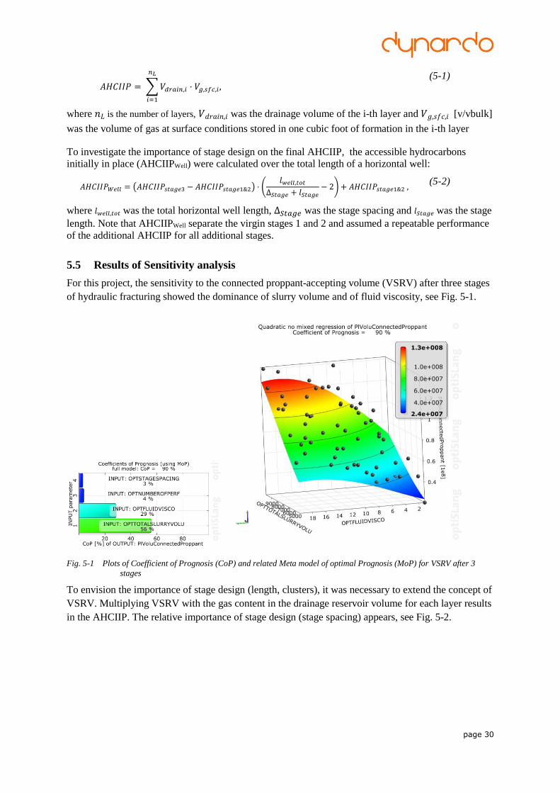
page 30
𝐴𝐻𝐶𝐼𝐼𝑃 = ∑𝑉𝑑𝑟𝑎𝑖𝑛,𝑖 ⋅ 𝑉𝑔,𝑠𝑓𝑐,𝑖
𝑛𝐿
𝑖=1
, (5-1)
where 𝑛𝐿 is the number of layers, 𝑉𝑑𝑟𝑎𝑖𝑛,𝑖 was the drainage volume of the i-th layer and 𝑉𝑔,𝑠𝑓𝑐,𝑖 [v/vbulk]
was the volume of gas at surface conditions stored in one cubic foot of formation in the i-th layer
To investigate the importance of stage design on the final AHCIIP, the accessible hydrocarbons
initially in place (AHCIIPWell) were calculated over the total length of a horizontal well:
𝐴𝐻𝐶𝐼𝐼𝑃𝑊𝑒𝑙𝑙 = (𝐴𝐻𝐶𝐼𝐼𝑃𝑠𝑡𝑎𝑔𝑒3 − 𝐴𝐻𝐶𝐼𝐼𝑃𝑠𝑡𝑎𝑔𝑒1&2) ⋅ (𝑙𝑤𝑒𝑙𝑙,𝑡𝑜𝑡
Δ𝑆𝑡𝑎𝑔𝑒 + 𝑙𝑆𝑡𝑎𝑔𝑒− 2) + 𝐴𝐻𝐶𝐼𝐼𝑃𝑠𝑡𝑎𝑔𝑒1&2 ,
(5-2)
where 𝑙𝑤𝑒𝑙𝑙,𝑡𝑜𝑡 was the total horizontal well length, Δ𝑆𝑡𝑎𝑔𝑒 was the stage spacing and 𝑙𝑆𝑡𝑎𝑔𝑒 was the stage
length. Note that AHCIIPWell separate the virgin stages 1 and 2 and assumed a repeatable performance
of the additional AHCIIP for all additional stages.
5.5 Results of Sensitivity analysis
For this project, the sensitivity to the connected proppant-accepting volume (VSRV) after three stages
of hydraulic fracturing showed the dominance of slurry volume and of fluid viscosity, see Fig. 5-1.
Fig. 5-1 Plots of Coefficient of Prognosis (CoP) and related Meta model of optimal Prognosis (MoP) for VSRV after 3
stages
To envision the importance of stage design (length, clusters), it was necessary to extend the concept of
VSRV. Multiplying VSRV with the gas content in the drainage reservoir volume for each layer results
in the AHCIIP. The relative importance of stage design (stage spacing) appears, see Fig. 5-2.
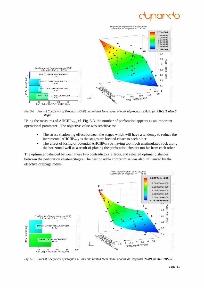
page 31
Fig. 5-2 Plots of Coefficient of Prognosis (CoP) and related Meta model of optimal prognosis (MoP) for AHCIIP after 3
stages
Using the measures of AHCIIPWell, cf. Fig. 5-3, the number of perforation appears as an important
operational parameter. The objective value was sensitive to:
The stress shadowing effect between the stages which will have a tendency to reduce the
incremental AHCIIPWell as the stages are located closer to each other
The effect of losing of potential AHCIIPWell by having too much unstimulated rock along
the horizontal well as a result of placing the perforation clusters too far from each other
The optimizer balanced between these two contradictory effects, and selected optimal distances
between the perforation clusters/stages. The best possible compromise was also influenced by the
effective drainage radius.
Fig. 5-3 Plots of Coefficient of Prognosis (CoP) and related Meta model of optimal Prognosis (MoP) for AHCIIPWell
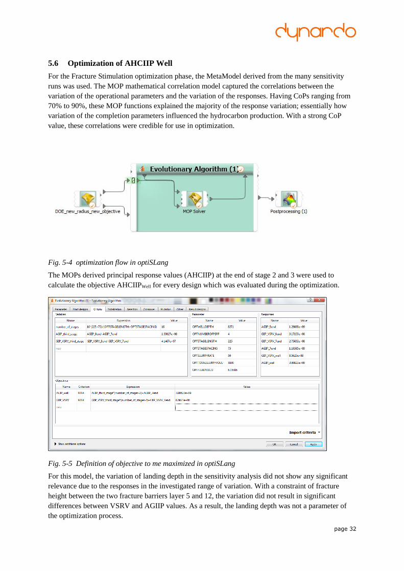
page 32
5.6 Optimization of AHCIIP Well
For the Fracture Stimulation optimization phase, the MetaModel derived from the many sensitivity
runs was used. The MOP mathematical correlation model captured the correlations between the
variation of the operational parameters and the variation of the responses. Having CoPs ranging from
70% to 90%, these MOP functions explained the majority of the response variation; essentially how
variation of the completion parameters influenced the hydrocarbon production. With a strong CoP
value, these correlations were credible for use in optimization.
Fig. 5-4 optimization flow in optiSLang
The MOPs derived principal response values (AHCIIP) at the end of stage 2 and 3 were used to
calculate the objective AHCIIPWell for every design which was evaluated during the optimization.
Fig. 5-5 Definition of objective to me maximized in optiSLang
For this model, the variation of landing depth in the sensitivity analysis did not show any significant
relevance due to the responses in the investigated range of variation. With a constraint of fracture
height between the two fracture barriers layer 5 and 12, the variation did not result in significant
differences between VSRV and AGIIP values. As a result, the landing depth was not a parameter of
the optimization process.

page 33
Using the MOPs, the following values finally were optimized:
cluster per stage
stage length
distance between stages
slurry rate
slurry volume
fluid viscosity
The potential gains with these optimizations appeared significant at virtually the same completion
cost. The potential for doubling the AGIIPWell (proxy for EUR) was indicated.
5.7 Outlook how to balance between additional completion costs and EUR
Experience shows that the opportunity to significantly improve HCIIPVSRV_Well and AHCIIPWell is
limited if the available completion costs are fixed. There appears to be a significant opportunity to
potential to improve with inventments in completion. But we need to check that the increase of
completion cost’s of hydraulic fracturing will not overprint the benefit from optimization of accessible
HCIIP.
Of course that only occur if the additional costs for well completion are not covered by the additional
oil and gas production. To evaluate the possible conflict, the optimization needs to be enlarged due to
cost function as well as revenue function out of the additional hydrocarbons. In order to do so we need
revenue estimations for additional oil and gas production as well as completion costs (UDC)
estimations for the additional stage designs and slurry volume.
To use suitable correlation between AHCIIPWell and estimated ultimate recovery (EUR) it is
recommended to calculate multiple wells nearby the calibration well using the MOP to calculate
AHCIIPWell and extract a correlation between AHCIIPWell and estimated EUR of the wells.
Having cost functions in place optiSlang can be used to calculate the Pareto Frontier, which represents
all completion designs were additional improvement of hydrocarbon production can only be achieved
with additional investments in completion. Fig. 5-6 shows a demo Pareto Frontier calculated with the
help of the MOP using anonymised correlations between AHCIIPWell, EUR and dummy cost functions.
Having such kind of Pareto Frontier decisions can be made regarding operational parameters in
relation to increase of completion costs and EUR at the same time.To deal with the Pareto Frontier as
an example three base scenarios are possible:
- optimize EUR to the maximal values and check completion costs
- what is the best possible EUR without increase of current completion costs
- or minimize completion costs keeping current EUR of current
- completion scenario
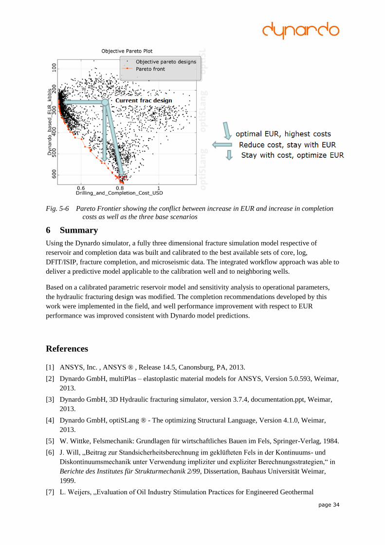
page 34
Fig. 5-6 Pareto Frontier showing the conflict between increase in EUR and increase in completion
costs as well as the three base scenarios
6 Summary
Using the Dynardo simulator, a fully three dimensional fracture simulation model respective of
reservoir and completion data was built and calibrated to the best available sets of core, log,
DFIT/ISIP, fracture completion, and microseismic data. The integrated workflow approach was able to
deliver a predictive model applicable to the calibration well and to neighboring wells.
Based on a calibrated parametric reservoir model and sensitivity analysis to operational parameters,
the hydraulic fracturing design was modified. The completion recommendations developed by this
work were implemented in the field, and well performance improvement with respect to EUR
performance was improved consistent with Dynardo model predictions.
References
[1] ANSYS, Inc. , ANSYS ® , Release 14.5, Canonsburg, PA, 2013.
[2] Dynardo GmbH, multiPlas – elastoplastic material models for ANSYS, Version 5.0.593, Weimar,
2013.
[3] Dynardo GmbH, 3D Hydraulic fracturing simulator, version 3.7.4, documentation.ppt, Weimar,
2013.
[4] Dynardo GmbH, optiSLang ® - The optimizing Structural Language, Version 4.1.0, Weimar,
2013.
[5] W. Wittke, Felsmechanik: Grundlagen für wirtschaftliches Bauen im Fels, Springer-Verlag, 1984.
[6] J. Will, „Beitrag zur Standsicherheitsberechnung im geklüfteten Fels in der Kontinuums- und
Diskontinuumsmechanik unter Verwendung impliziter und expliziter Berechnungsstrategien,“ in
Berichte des Institutes für Strukturmechanik 2/99, Dissertation, Bauhaus Universität Weimar,
1999.
[7] L. Weijers, „Evaluation of Oil Industry Stimulation Practices for Engineered Geothermal

page 35
Systems, Pinnacle Report DOE-PS36-04GO94001,“ October 2010.
[8] J. Will und R. Schlegel, „Simulation of hydraulic fracturing of jointed rock,“ in Proceedings of
European Conference on Fracture, Dresden, 2010.
[9] J. C. Simo und T. J. Hughes, Computational Inelasticity, Springer, 1998.
[10] K. J. Bathe, Finite element procedures, Prentice Hall, 1985.
[11] M. Jirasek und Z. P. Bazant, Inelastic Analysis of Structures, John Wiley & Sons, 2001.
[12] R. Pölling, Eine praxisnahe, schädigungsorientierte Materialbeschreibung von Stahlbeton für
Strukturanalysen, Dissertation, Ruhr-Universität Bochum, 2000.
[13] N. Barton, S. Bandis and K. Bakhtar, "Strength, deformation and conductivity coupling of rock
joints," International Journal of Rock Mechanics and Mining Sciences & Geomechanics
Abstracts, vol. 22, no. 3, p. 121–140, June 1985.
[14] M. T. Z. Iragorre, Thermo-hydro-mechanical analysis of joints a theoretical and experimental
study, Barcelona: Phd-Thesis, Univesitat politècnica de Catalunya, 2010.
[15] A. F. Gangi, "Variation of whole and fractured porous rock permeability with confining
pressure," International Journal of Rock Mechanics and Mining Sciences & Geomechanics
Abstracts, vol. 15, no. 5, pp. 249-257, 1978.
[16] T. Most und J. Will, „Efficient sensitivity analysis for virtual prototyping,“ in Proceedings of the
6th European Congress on Computational Methods in Applied Sciences and Engineering,
Vienna, 2012.
Top Related