


Languages
Pages
Legal

OntologiesReasoningComponentsAgentsSimulations
Problem Solving throughProblem Solving throughState Space SearchState Space Search
Jacques Robin
OutlineOutline
Search Agent Formulating Decision Problems as Navigating State Space to Find Goal
State Generic Search Algorithm Specific Algorithms
Breadth-First Search Uniform Cost Search Depth-First Search Backtracking Search Iterative Deepening Search Bi-Directional Search Comparative Table
Limitations and Difficulties Repeated States Partial Information
Search AgentsSearch Agents
Generic decision problem to be solved by an agent: Among all possible action sequences that I can execute, which ones will result in changing the environment from its current state, to another state that matches my goal?
Additional optimization problem: Among those action sequences that will change the environment from its current state
to a goal state which one can be executed at minimum cost? or which one leads to a state with maximum utility?
Search agent solves this decision problem by a generate and test approach: Given the environment model, generate one by one (all) the possible states (the state space) of the environment
reachable through all possible action sequences from the current state, test each generated state to determine whether it satisfies the goal or maximize utility
Navigation metaphor: The order of state generation is viewed as navigating the entire environment state
space
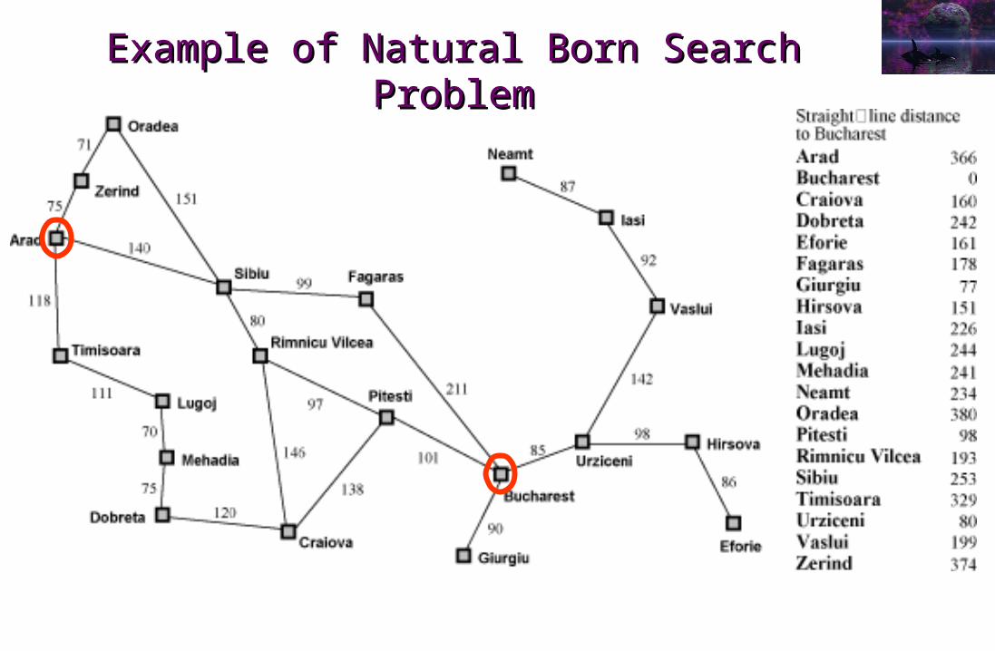
Example of Natural Born Search ProblemExample of Natural Born Search Problem
Example of Applying Navigation MetaphorExample of Applying Navigation Metaphorto Arbitrary Decision Problemto Arbitrary Decision Problem
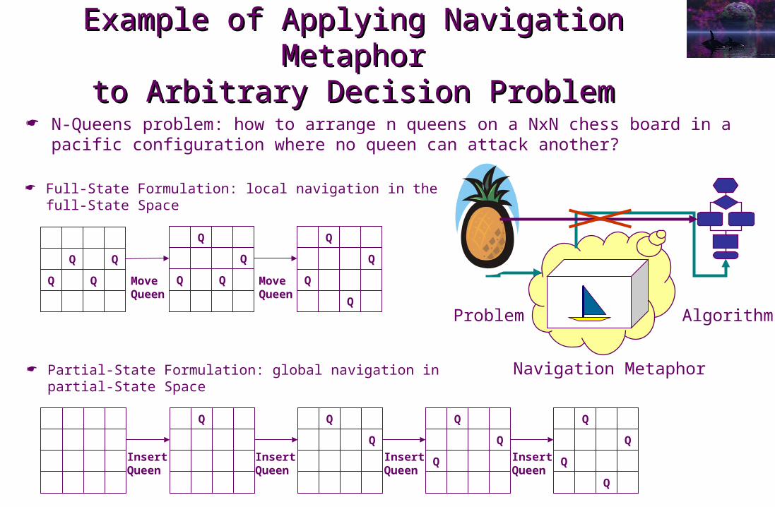
N-Queens problem: how to arrange n queens on a NxN chess board in a pacific configuration where no queen can attack another?
Navigation Metaphor
Problem Algorithm
Q Q
Q
Q
Q
Q
Q
Q
Q
Q
InsertQueen
InsertQueen
InsertQueen
InsertQueen
Q
Q
Q Q
Q
Q
Q
Q
Q Q
Q Q MoveQueen
MoveQueen
Full-State Formulation: local navigation in thefull-State Space
Partial-State Formulation: global navigation in partial-State Space
Search Problem TaxonomySearch Problem Taxonomy
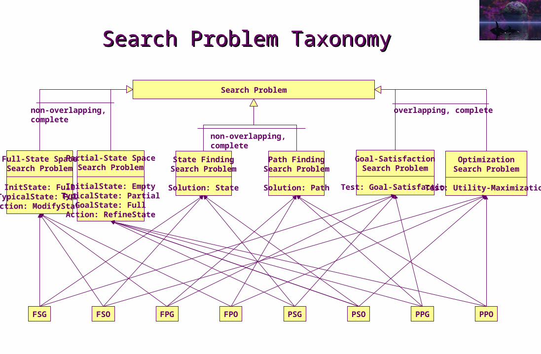
Search Problem
Full-State SpaceSearch Problem
InitState: FullTypicalState: Full
Action: ModifyState
Partial-State SpaceSearch Problem
InitialState: EmptyTypicalState: Partial
GoalState: FullAction: RefineState
non-overlapping,complete
overlapping, complete
Goal-SatisfactionSearch Problem
Test: Goal-Satisfaction
OptimizationSearch Problem
Test: Utility-Maximization
PPGFSG FPGFSO FPO PSOPSG PPO
non-overlapping, complete
State FindingSearch Problem
Solution: State
Path FindingSearch Problem
Solution: Path
Search TreeSearch Tree
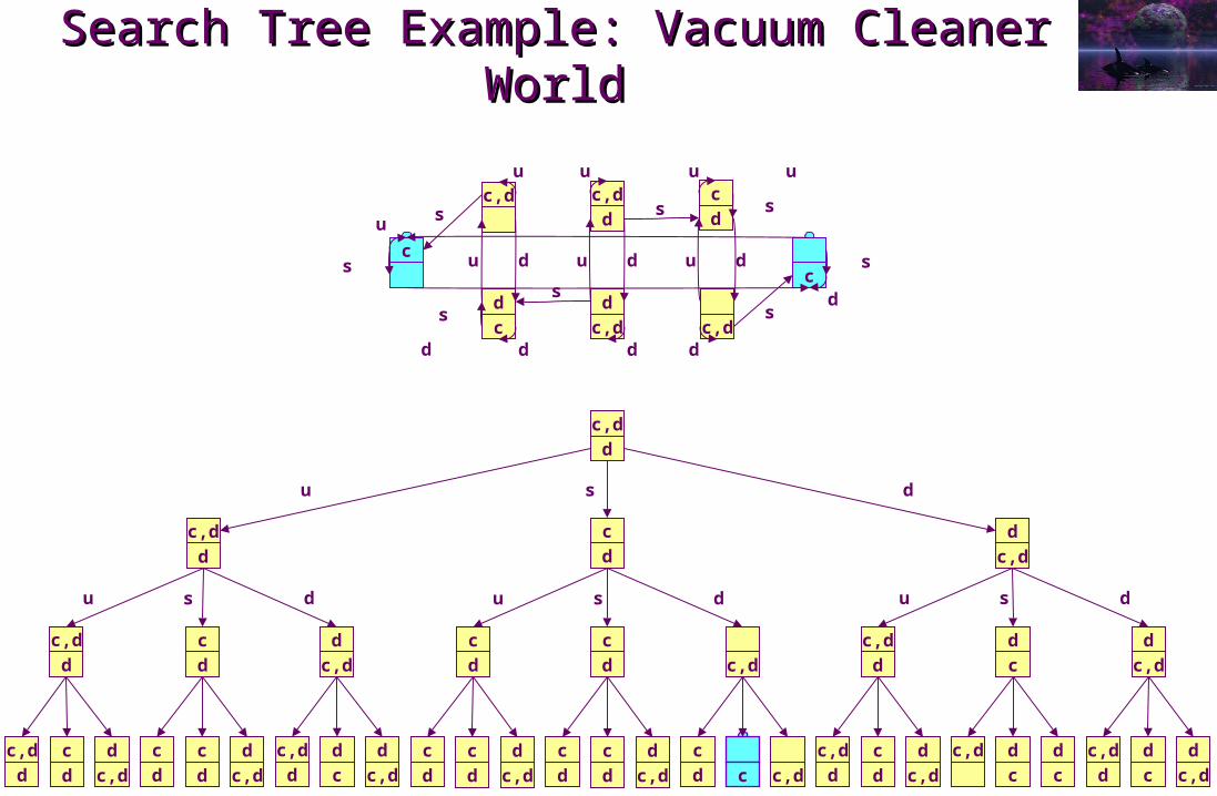
The state space can be represented as a search tree Each search tree node represents an environment state Each search tree arc represents an action changing the environment from its
source node to its target node Each node or arc can be associated to a utility or cost Each path from the tree root to another tree node represents an action sequence Some search tree node leaves represent goal states The problem of navigating the state space then becomes one of generating and
maintaining a search tree until a solution node or path is generated The problem search tree:
An abstract concept that contains one node for each possible environment state Can be infinite
The algorithm search tree: A concrete data structure A subset of the problem search tree that contains only the nodes generated and
maintained (i.e., explored) at the current point during the algorithm execution (always finite)
Problem search tree branching factor: average number of actions available to the agent in each state
Algorithm effective branching factor: average number of nodes effectively generated as successors of each node during search
Search Tree Example: Vacuum Cleaner Search Tree Example: Vacuum Cleaner WorldWorld
c,d
d
c
d
c
d
c,d
d
d
c,d
c,d
dc
d
d
c,d
c
d c,d
d
c
c,d
d
d
c,d
c
dc
d
d
c,d
c,d
dc
d
d
c,d
c,d
dd
c
d
c,dc
dc
d
d
c,d
c
dc
d
d
c,d
c
d c c,d
c,d
dc
d
d
c,d
c,d d
c
c,d
d
d
c
d
c
d
c,d
u s d
u ds u ds u ds
c,d
d
c
d
d
c,d c,d
c
d
c
c,d
c
u
uu u
d
ddd
s
s
d
s
u
s
d
u
dudu
s
s
ss
Search MethodsSearch Methods
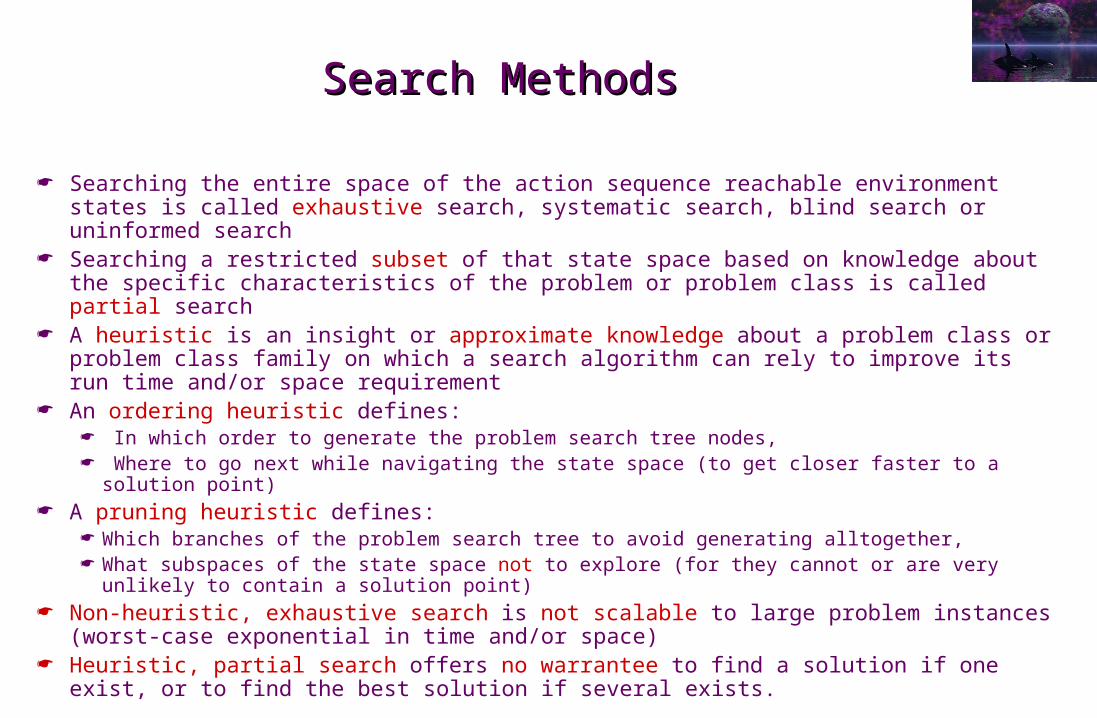
Searching the entire space of the action sequence reachable environment states is called exhaustive search, systematic search, blind search or uninformed search
Searching a restricted subset of that state space based on knowledge about the specific characteristics of the problem or problem class is called partial search
A heuristic is an insight or approximate knowledge about a problem class or problem class family on which a search algorithm can rely to improve its run time and/or space requirement
An ordering heuristic defines: In which order to generate the problem search tree nodes, Where to go next while navigating the state space (to get closer faster to a solution
point) A pruning heuristic defines:
Which branches of the problem search tree to avoid generating alltogether, What subspaces of the state space not to explore (for they cannot or are very unlikely to
contain a solution point) Non-heuristic, exhaustive search is not scalable to large problem instances
(worst-case exponential in time and/or space) Heuristic, partial search offers no warrantee to find a solution if one exist, or to
find the best solution if several exists.
Formulating a Agent Decision ProblemFormulating a Agent Decision Problemas a Search Problemas a Search Problem
Define abstract format of a generic environment state, ex., a class C Define the initial state, ex., a specific object of class C Define the successor operation:
Takes as input a state or state set S and an action A Returns the state or state set R resulting from the agent executing A in S
Together, these 3 elements constitute an intentional representation of the state space The search algorithm transforms this intentional representation into an
extensional one, by repeatedly applying the successor operation starting from the initial state
Define a boolean operation testing whether a state is a goal, ex., a method of C
For optimization problems: additionally define a operation that returns the cost or utility of an action or state
Problem Formulation Most Crucial FactorProblem Formulation Most Crucial Factorof Search Efficiencyof Search Efficiency
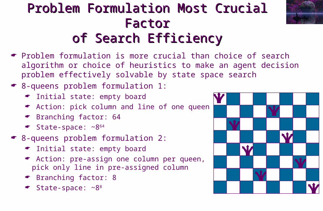
Problem formulation is more crucial than choice of search algorithm or choice of heuristics to make an agent decision problem effectively solvable by state space search
8-queens problem formulation 1: Initial state: empty board Action: pick column and line of one queen Branching factor: 64 State-space: ~864
8-queens problem formulation 2: Initial state: empty board Action: pre-assign one column per queen,
pick only line in pre-assigned column Branching factor: 8 State-space: ~88
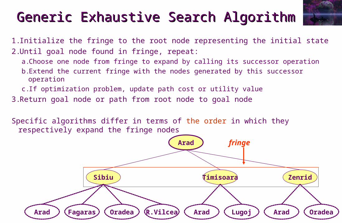
Generic Exhaustive Search AlgorithmGeneric Exhaustive Search Algorithm
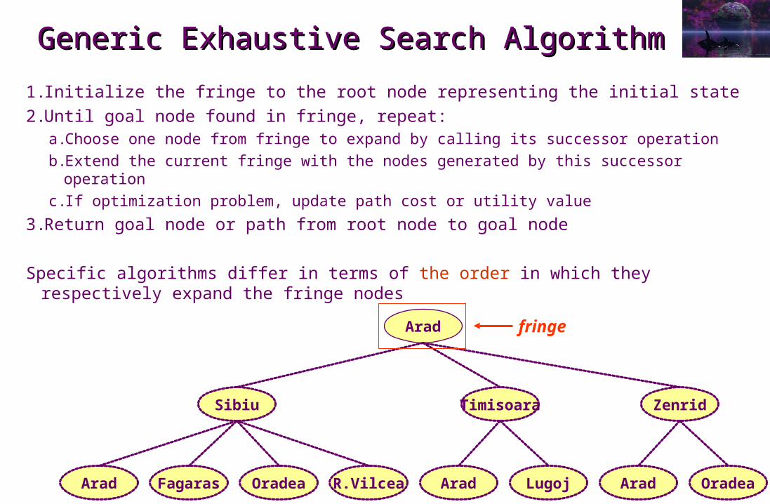
1.Initialize the fringe to the root node representing the initial state2.Until goal node found in fringe, repeat:
a.Choose one node from fringe to expand by calling its successor operationb.Extend the current fringe with the nodes generated by this successor operationc. If optimization problem, update path cost or utility value
3.Return goal node or path from root node to goal node
Specific algorithms differ in terms of the order in which they respectively expand the fringe nodes
Arad Fagaras Oradea R.Vilcea Arad Lugoj Arad Oradea
Sibiu Timisoara Zenrid
Arad fringe
Generic Exhaustive Search AlgorithmGeneric Exhaustive Search Algorithm
1.Initialize the fringe to the root node representing the initial state2.Until goal node found in fringe, repeat:
a.Choose one node from fringe to expand by calling its successor operationb.Extend the current fringe with the nodes generated by this successor operationc. If optimization problem, update path cost or utility value
3.Return goal node or path from root node to goal node
Specific algorithms differ in terms of the order in which they respectively expand the fringe nodes
Arad Fagaras Oradea R.Vilcea Arad Lugoj Arad Oradea
Sibiu Timisoara Zenrid
Arad fringe
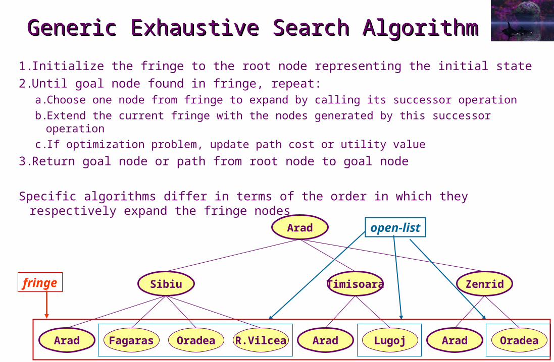
Generic Exhaustive Search AlgorithmGeneric Exhaustive Search Algorithm
1.Initialize the fringe to the root node representing the initial state2.Until goal node found in fringe, repeat:
a.Choose one node from fringe to expand by calling its successor operationb.Extend the current fringe with the nodes generated by this successor operationc. If optimization problem, update path cost or utility value
3.Return goal node or path from root node to goal node
Specific algorithms differ in terms of the order in which they respectively expand the fringe nodes
Arad Fagaras Oradea R.Vilcea Arad Lugoj Arad Oradea
Sibiu Timisoara Zenrid
Arad open-list
fringe
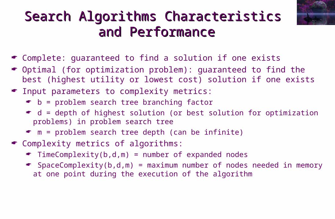
Search Algorithms CharacteristicsSearch Algorithms Characteristics and Performance and Performance
Complete: guaranteed to find a solution if one exists Optimal (for optimization problem): guaranteed to find the best (highest
utility or lowest cost) solution if one exists Input parameters to complexity metrics:
b = problem search tree branching factor d = depth of highest solution (or best solution for optimization problems) in
problem search tree m = problem search tree depth (can be infinite)
Complexity metrics of algorithms: TimeComplexity(b,d,m) = number of expanded nodes SpaceComplexity(b,d,m) = maximum number of nodes needed in memory at
one point during the execution of the algorithm
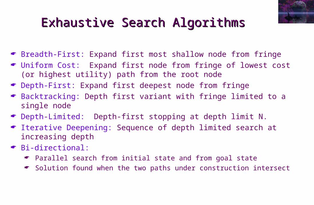
Exhaustive Search AlgorithmsExhaustive Search Algorithms
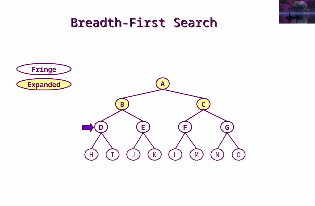
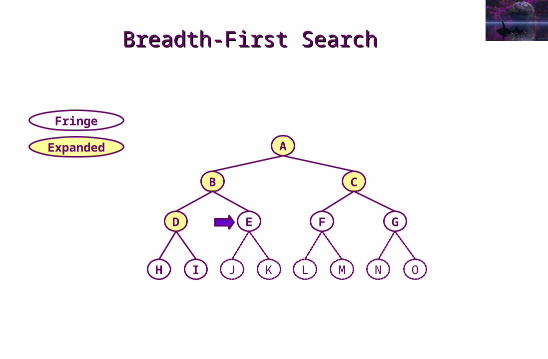
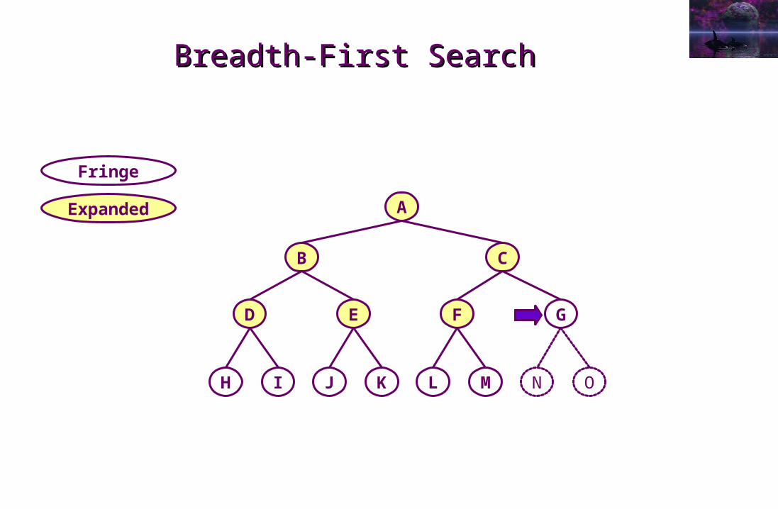
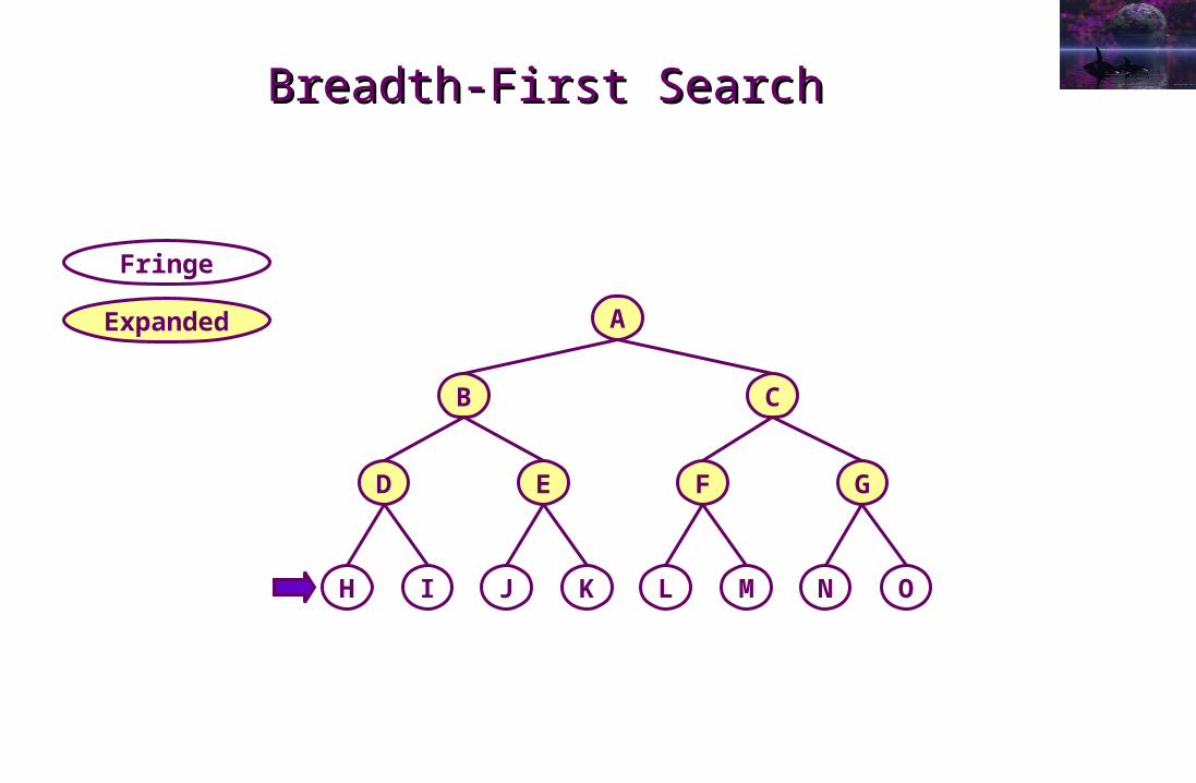
Breadth-First: Expand first most shallow node from fringe Uniform Cost: Expand first node from fringe of lowest cost (or highest
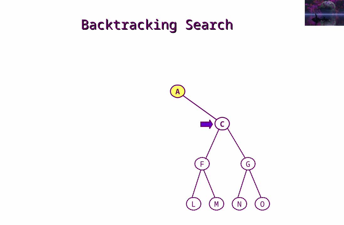
utility) path from the root node Depth-First: Expand first deepest node from fringe Backtracking: Depth first variant with fringe limited to a single node Depth-Limited: Depth-first stopping at depth limit N. Iterative Deepening: Sequence of depth limited search at increasing
depth Bi-directional:
Parallel search from initial state and from goal state Solution found when the two paths under construction intersect
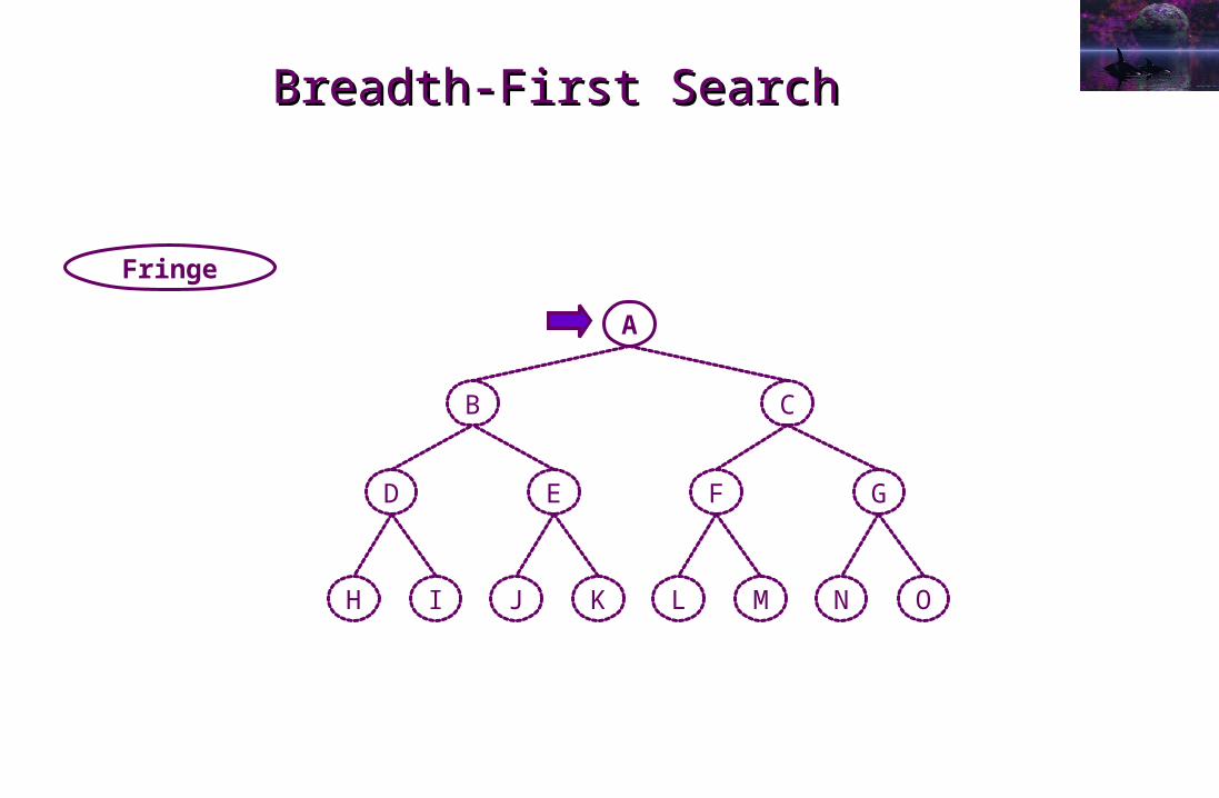
Breadth-First SearchBreadth-First Search
A
B C
E FD G
K MI OJ LH N
Fringe
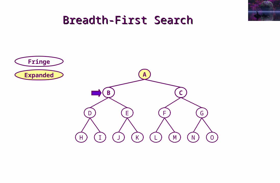
Breadth-First SearchBreadth-First Search
A
B C
E FD G
K MI OJ LH N
Fringe
Expanded

Breadth-First SearchBreadth-First Search
A
B C
E FD G
K MI OJ LH N
Fringe
Expanded
Breadth-First SearchBreadth-First Search
A
B C
E FD G
K MI OJ LH N
Fringe
Expanded
Breadth-First SearchBreadth-First Search
A
B C
E FD G
K MI OJ LH N
Fringe
Expanded

Breadth-First SearchBreadth-First Search
A
B C
E FD G
K MI OJ LH N
Fringe
Expanded
Breadth-First SearchBreadth-First Search
A
B C
E FD G
K MI OJ LH N
Fringe
Expanded
Breadth-First SearchBreadth-First Search
A
B C
E FD G
K MI OJ LH N
Fringe
Expanded
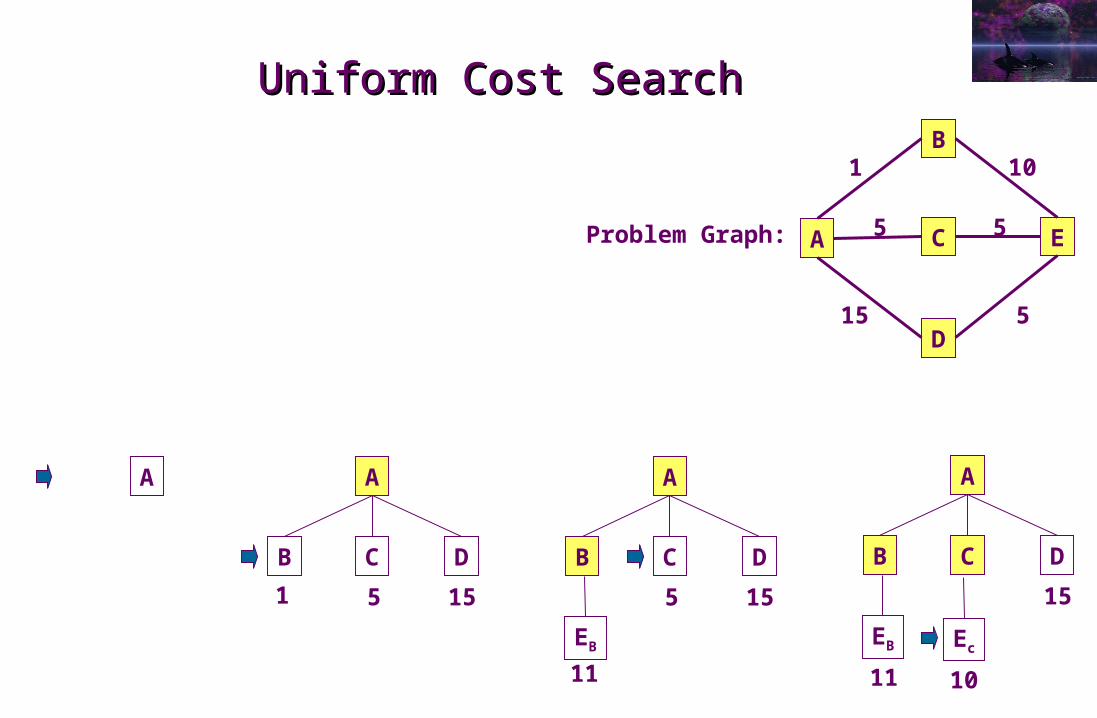
Uniform Cost SearchUniform Cost Search
A C E
B
D
Problem Graph:
1 10
515
5 5
A
B C D
1 5 15
11
A
B C D
5 15
EB
A
B C D
11 10
15
EB Ec
A
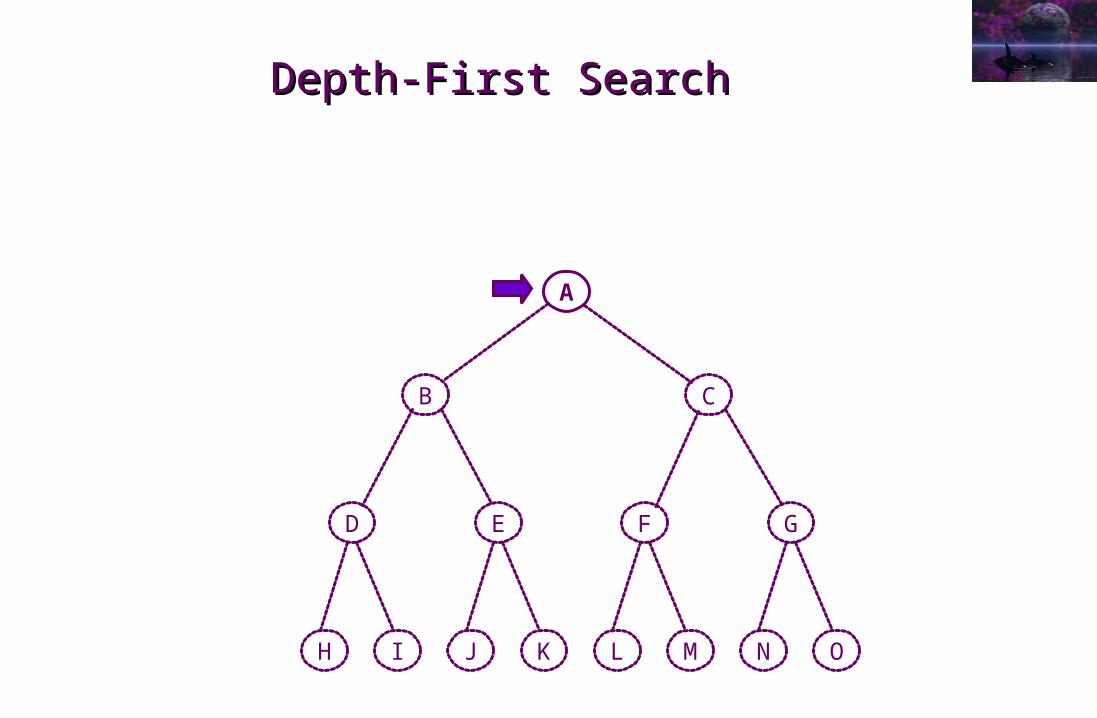
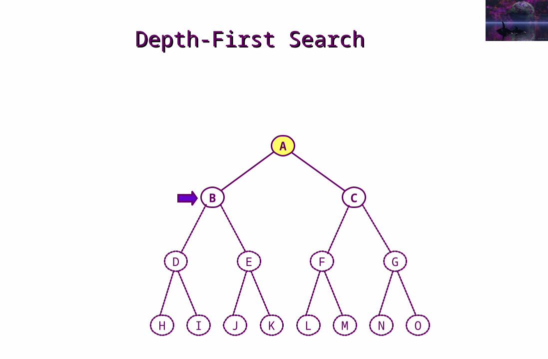
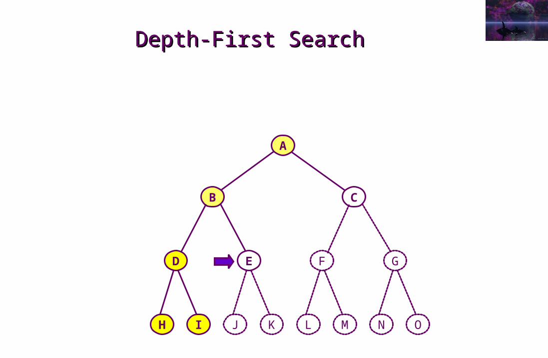
Depth-First SearchDepth-First Search
A
B C
E FD G
J LH NK MI O
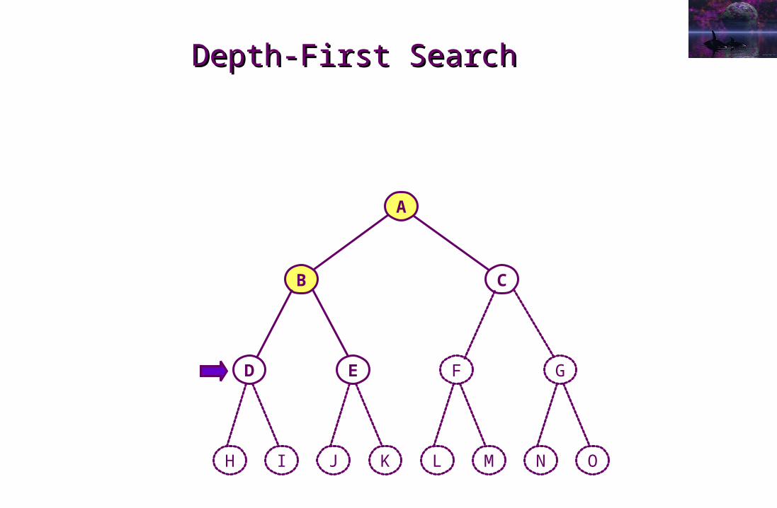
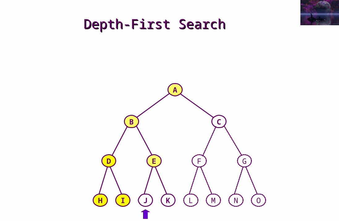
Depth-First SearchDepth-First Search
A
B C
E FD G
J LH NK MI O
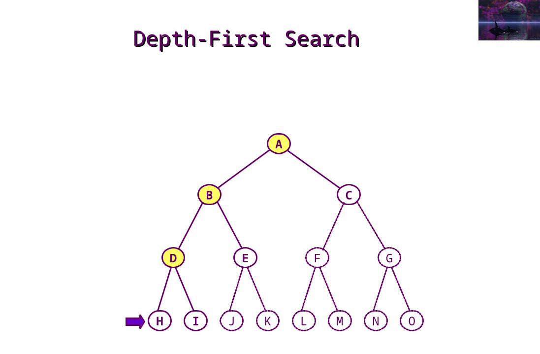
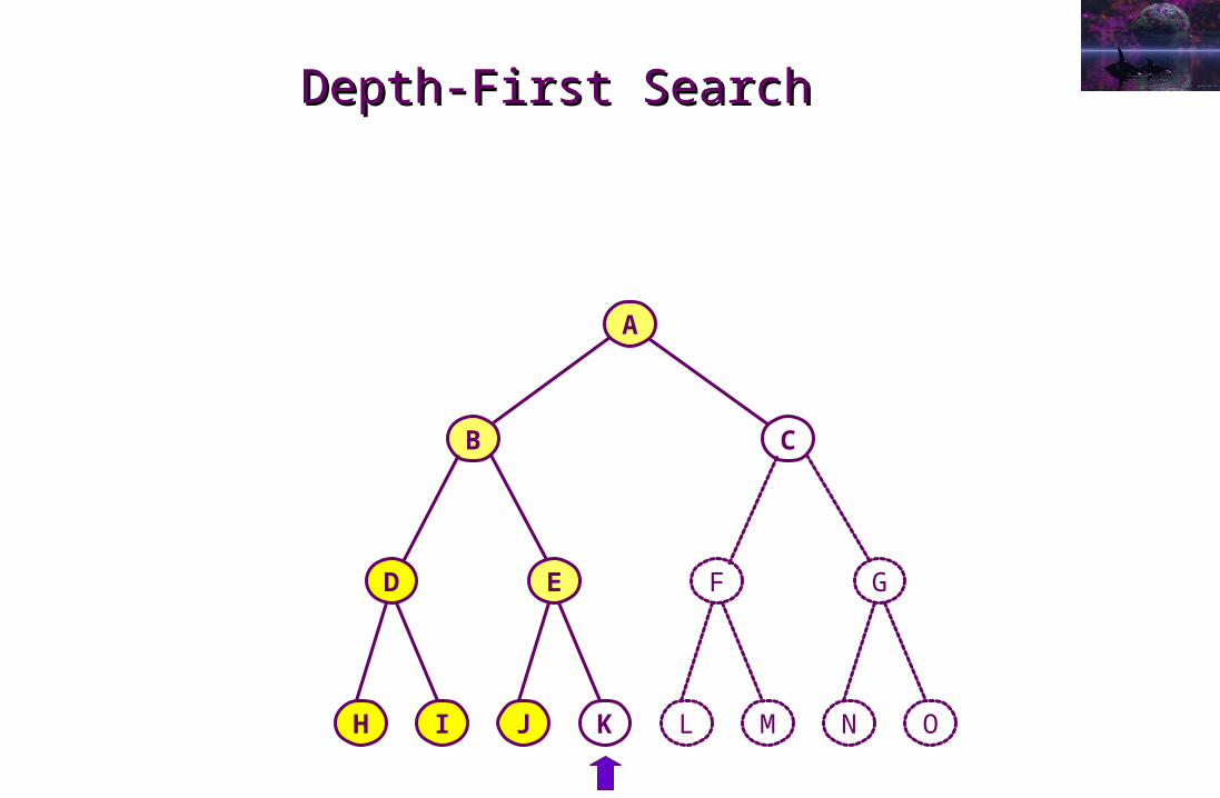
Depth-First SearchDepth-First Search
A
B C
E FD G
J LH NK MI O
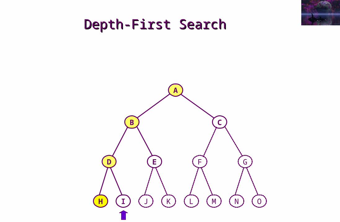
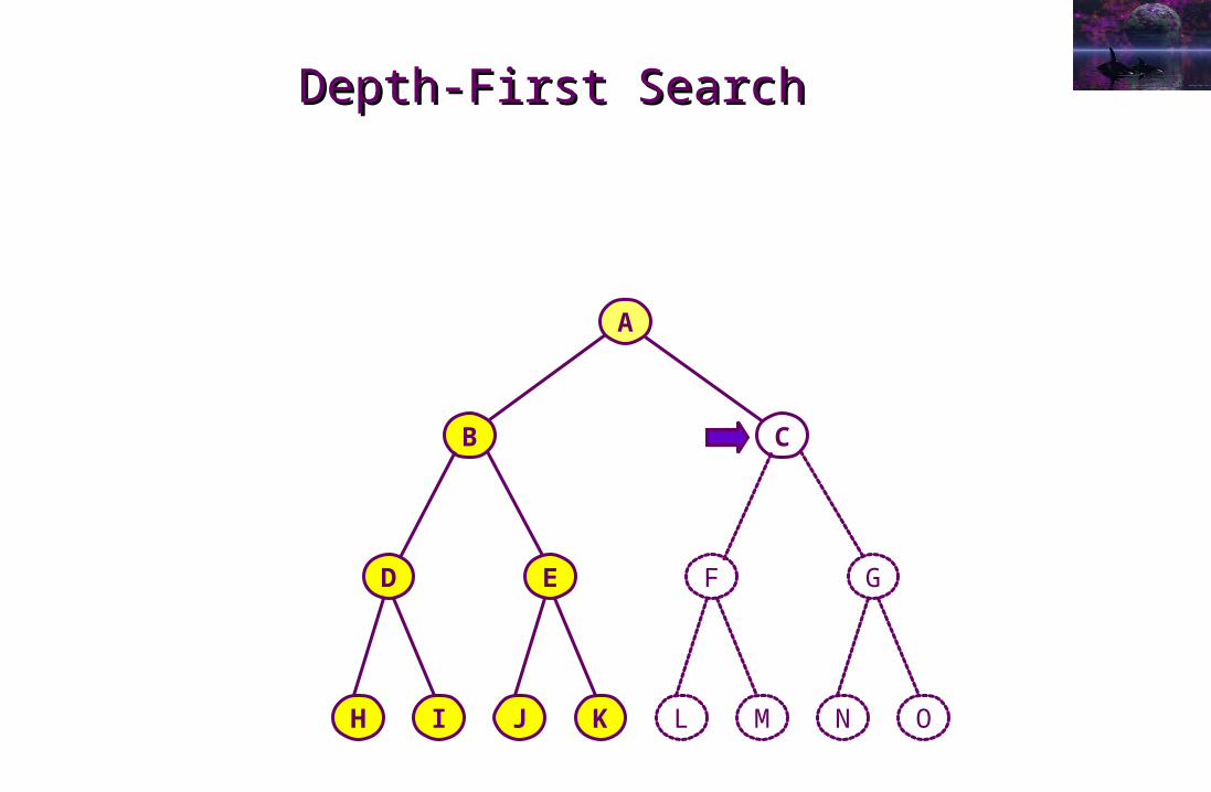
Depth-First SearchDepth-First Search
A
B C
E FD G
J LH NK MI O
Depth-First SearchDepth-First Search
A
B C
E FD G
J LH NK MI O
Depth-First SearchDepth-First Search
A
B C
E FD G
J LH NK MI O
Depth-First SearchDepth-First Search
A
B C
E FD G
J LH NK MI O
Depth-First SearchDepth-First Search
A
B C
E FD G
J LH NK MI O
Depth-First SearchDepth-First Search
A
B C
E FD G
J LH NK MI O
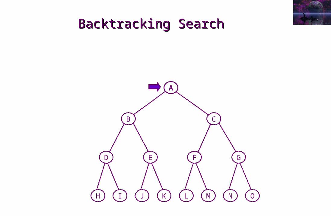
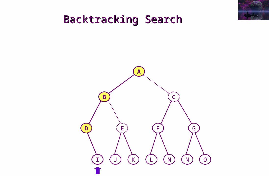
Backtracking SearchBacktracking Search
A
B C
E FD G
J LH NK MI O
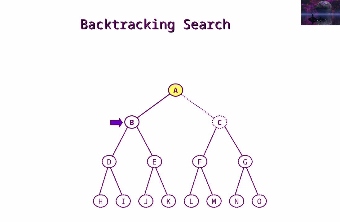
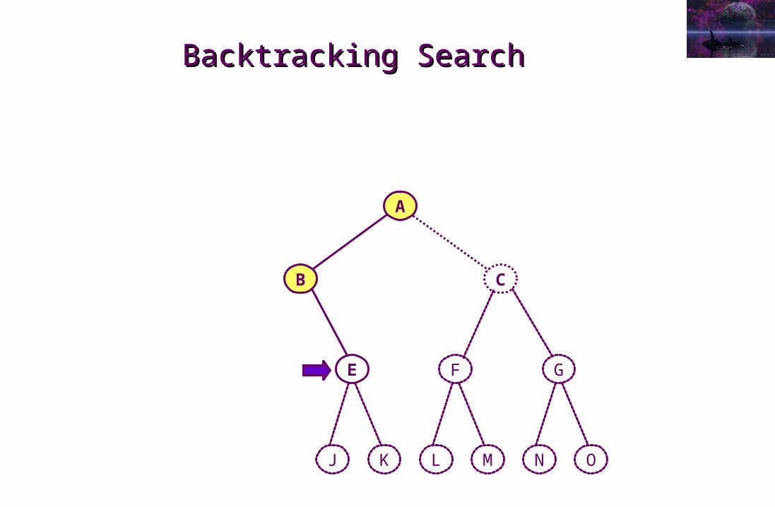
Backtracking SearchBacktracking Search
A
B C
E FD G
J LH NK MI O
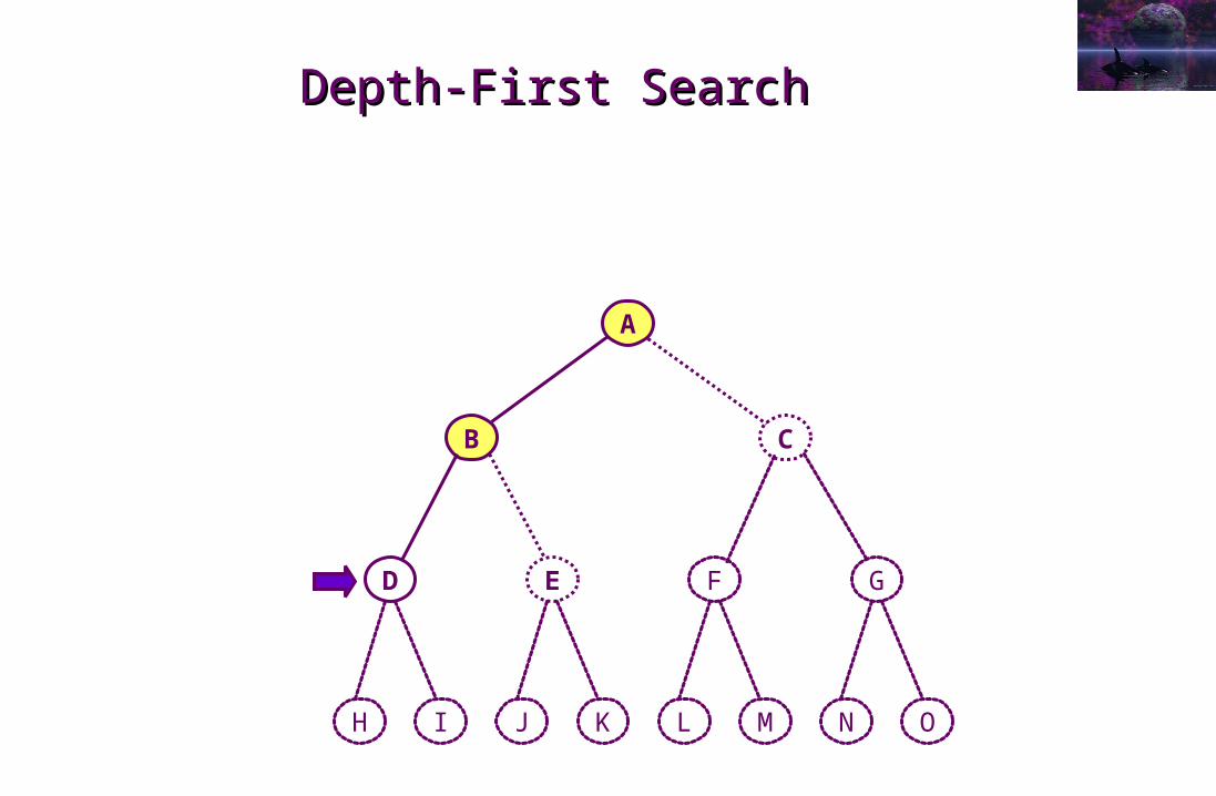
Depth-First SearchDepth-First Search
A
B C
E FD G
J LH NK MI O
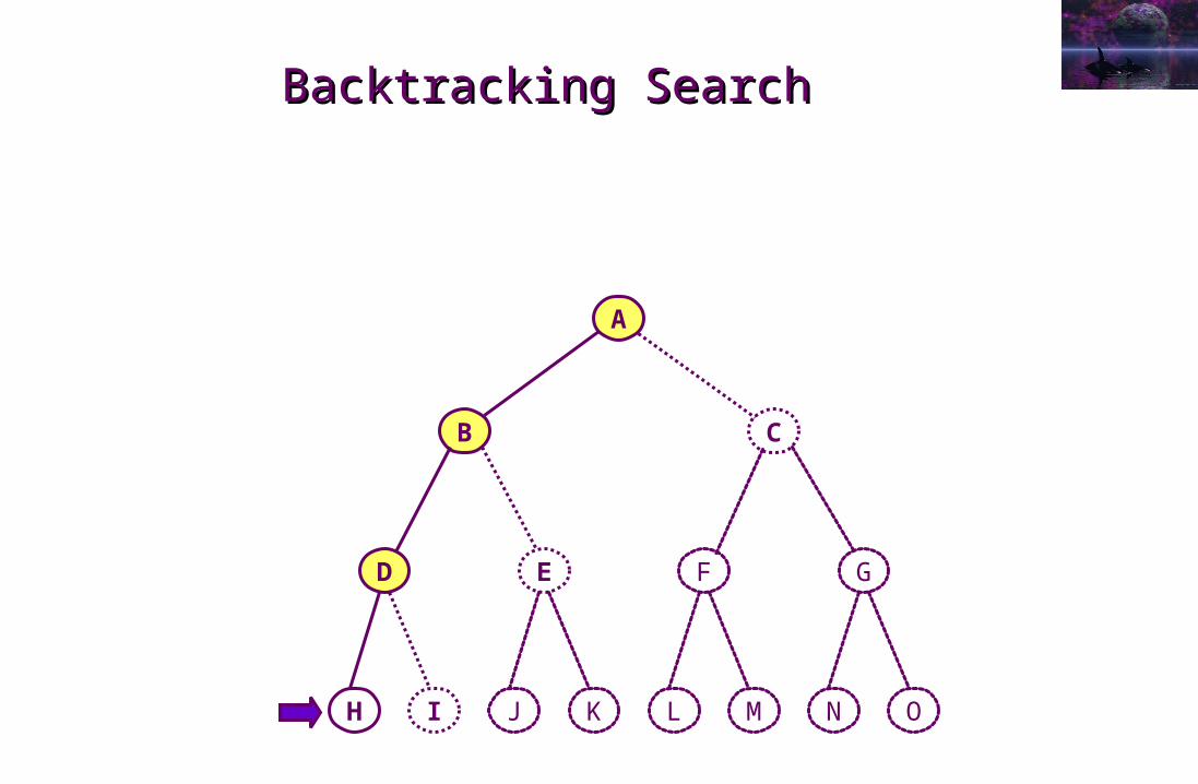
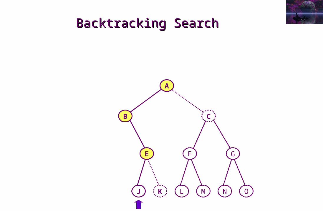
Backtracking SearchBacktracking Search
A
B C
E FD G
J LH NK MI O
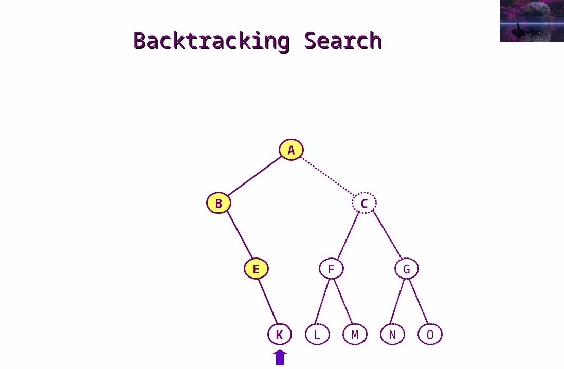
Backtracking SearchBacktracking Search
A
B C
E FD G
J L NK MI O
Backtracking SearchBacktracking Search
A
B C
E F G
J L NK M O
Backtracking SearchBacktracking Search
A
B C
E F G
J L NK M O
Backtracking SearchBacktracking Search
A
B C
E F G
L NK M O
Backtracking SearchBacktracking Search
A
C
F G
L NM O
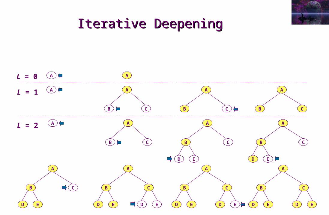
Iterative DeepeningIterative Deepening
A
A
B C
A
B C
D E D E
A
B C
D E
A
B C
D E D E
AL = 0
AL = 1 A
B C
A
B C
AL = 2 A
B C
A
B C
D E
A
B C
D E
A
B C
D E D E
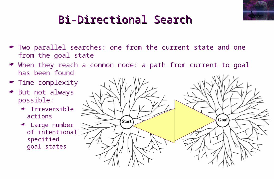
Bi-Directional SearchBi-Directional Search
Two parallel searches: one from the current state and one from the goal state
When they reach a common node: a path from current to goal has been found
Time complexity halved: O(bd/2) + O(bd/2) = O(bd/2) << O(bd) But not always
possible: Irreversible
actions Large number
of intentionallyspecifiedgoal states
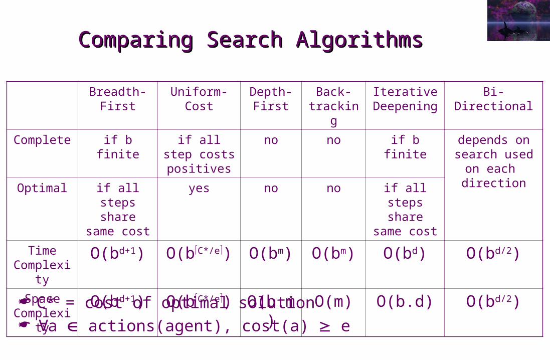
Comparing Search AlgorithmsComparing Search Algorithms
C* = cost of optimal solution a actions(agent), cost(a) e
Breadth-First
Uniform-Cost
Depth-First
Back-tracking
Iterative Deepening
Bi-Directional
Complete if b finite if all step costs
positives
no no if b finite depends on search used
on each directionOptimal if all steps
share same cost
yes no no if all steps share
same cost
Time Complexit
y
O(bd+1) O(bC*/e) O(bm) O(bm) O(bd) O(bd/2)
Space Complexit
y
O(bd+1) O(bC*/e) O(b.m)
O(m) O(b.d) O(bd/2)
Searching EnvironmentsSearching Environmentswith Repeated Stateswith Repeated States
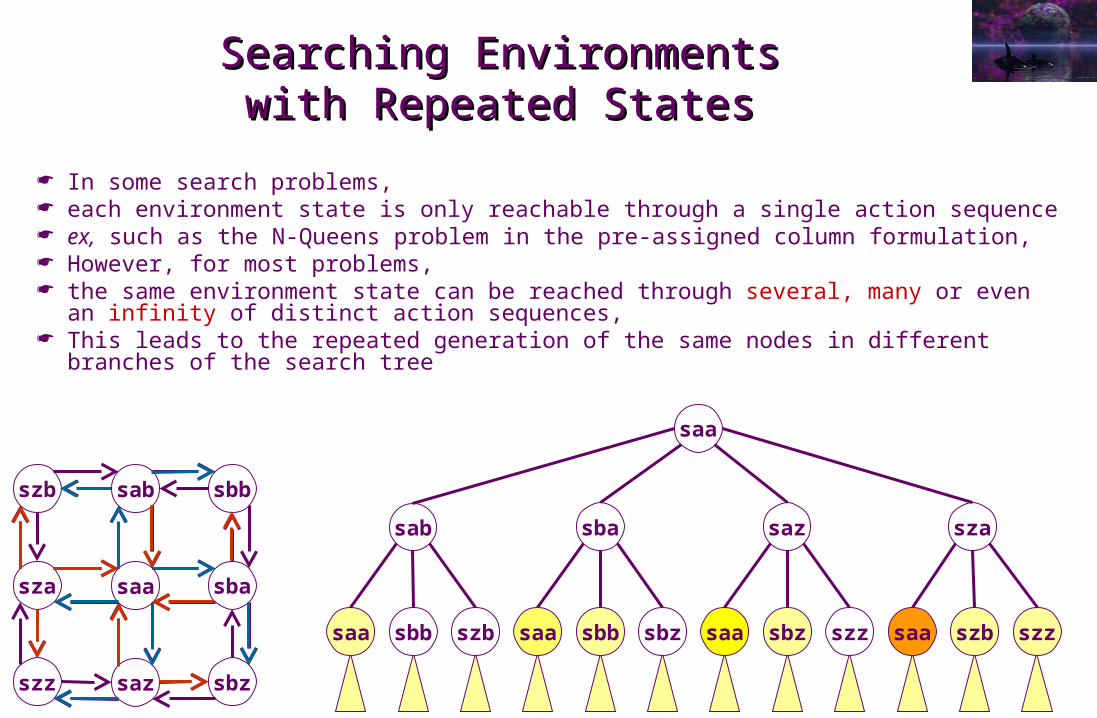
In some search problems, each environment state is only reachable through a single action sequence ex, such as the N-Queens problem in the pre-assigned column formulation, However, for most problems, the same environment state can be reached through several, many or even an
infinity of distinct action sequences, This leads to the repeated generation of the same nodes in different branches
of the search tree
saa
sab
saz
sba
sbb
sbz
sza
szb
szz
saa
sab sba szasaz
saa sbb saa sbb sbz saa sbz szz saaszb szb szz
Effects of Repeated States onEffects of Repeated States onExhaustive Search AlgorithmsExhaustive Search Algorithms
They must be modified to include test comparing newly generated nodes with already generated ones and prune the repeated ones from the frontier
Without such test: Breadth-first and uniform-cost search fill memory far sooner with repeated
nodes and likely before reaching the depth of the first goal node Depth-first and backtracking search can enter in deepening loop, never
returning even in the presence of shallow goal nodes With such test
Depth-first, backtracking and iterative deepening search loose their linear worst-case space complexity,
for any guarantee to avoid all loops may require keeping an exponential number of expanded nodes in memory,
in practice, the probability of loop occurrence is traded-off for size of the expanded node history
Heuristic Search:Heuristic Search:Definition and MotivationDefinition and Motivation
Definition: Non-exhaustive, partial state space search strategy, based on approximate heuristic knowledge of the search problem class (ex, n-queens,
Romania touring) or family (ex, unordered finite domain constraint solving) allowing to leave unexplored (prune) state space zones that are either guaranteed or
unlikely to contain a goal state (or a utility maximizing state or cost minimizing path) Note:
An algorithm that uses a fringe node ordering heuristic to generate a goal state faster, but is still ready to generate all state space states if necessary to find goal state i.e., an algorithm that does no pruning is not a heuristic search algorithm
Motivation: exhaustive search algorithms do not scale up, neither theoretically (exponential worst case time or space complexity) nor empirically (experimentally measured average case time or space complexity)
Heuristic search algorithms do scale up to very large problem instances, in some cases by giving up completeness and/or optimality
New data structure: heuristic function h(s) estimates the cost of the path from a fringe state s to a goal state
Best-First Global SearchBest-First Global Search
Keep all expanded states on the fringe just as exhaustive breadth-first search and uniform-cost search
Define an evaluation function f(s) that maps each state onto a number Expand the fringe in order of decreasing f(s) values Variations:
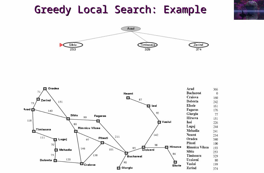
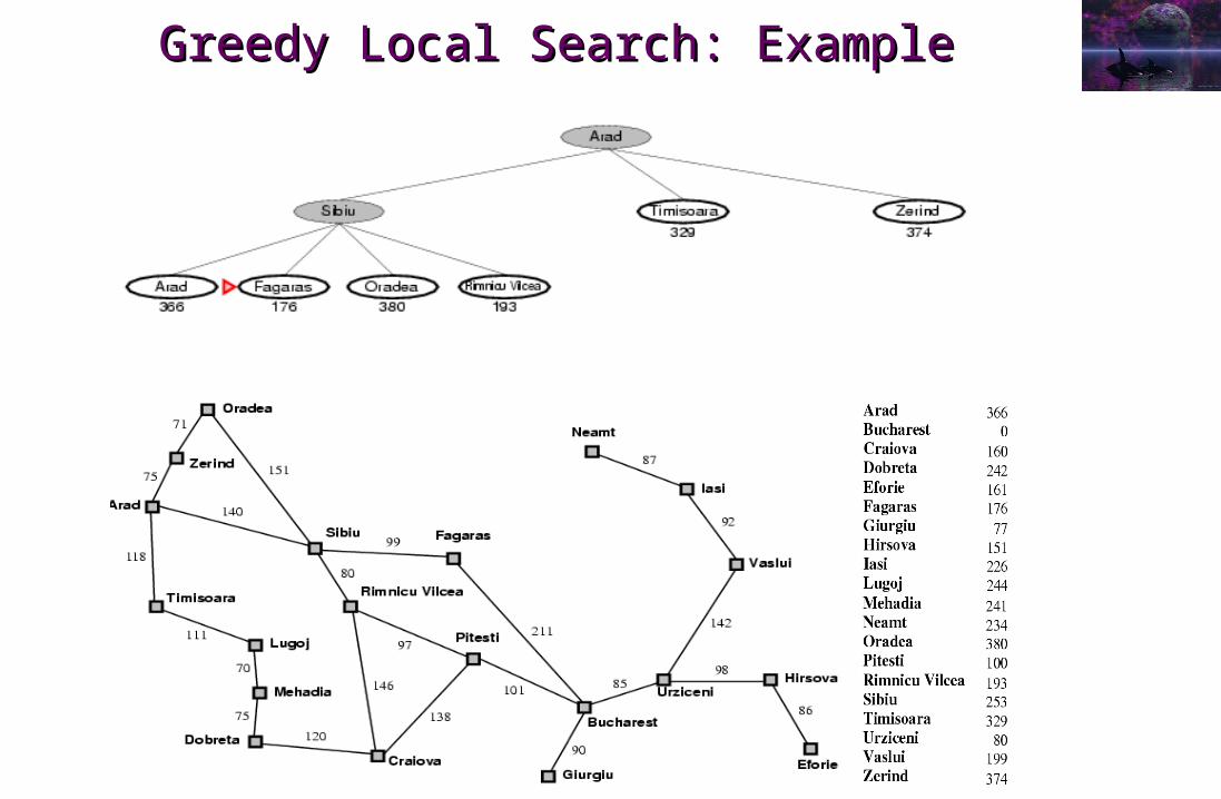
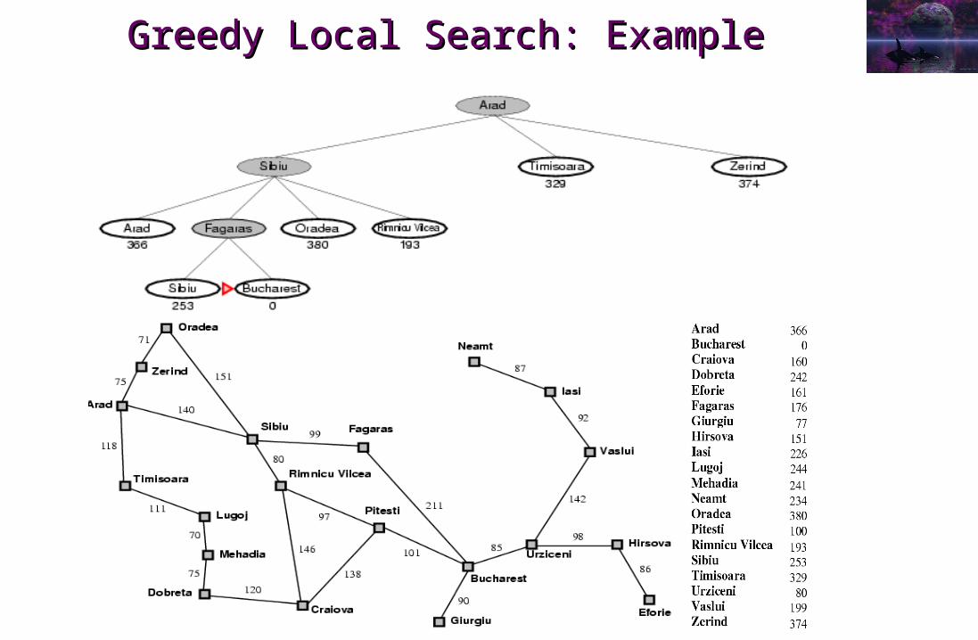
Greedy Global Search (also called Greedy Best-First Search) defines f(s) = h(s)
A* defines f(s) = g(s) + h(s) where g(s) is the real cost from the initial state to the state s, i.e., the value used to choose the state to expand in uniform cost search
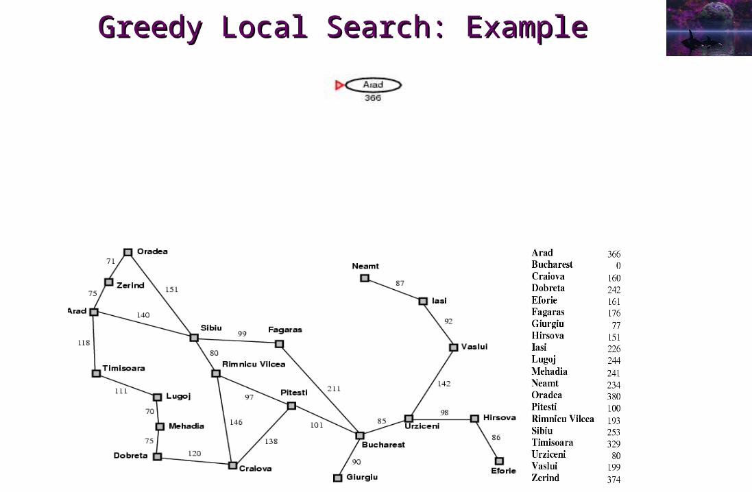
Greedy Local Search: ExampleGreedy Local Search: Example
Greedy Local Search: ExampleGreedy Local Search: Example
Greedy Local Search: ExampleGreedy Local Search: Example
Greedy Local Search: ExampleGreedy Local Search: Example
Greedy Local Search CharacteristicsGreedy Local Search Characteristics
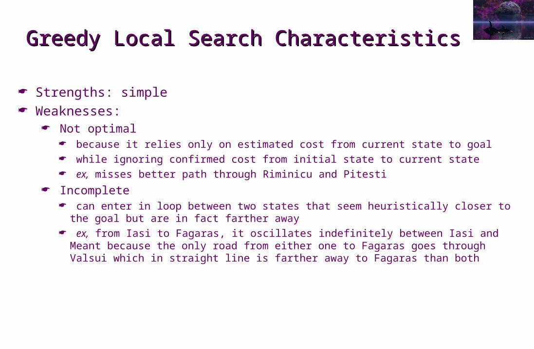
Strengths: simple Weaknesses:
Not optimal because it relies only on estimated cost from current state to goal while ignoring confirmed cost from initial state to current state ex, misses better path through Riminicu and Pitesti
Incomplete can enter in loop between two states that seem heuristically closer to the goal but
are in fact farther away ex, from Iasi to Fagaras, it oscillates indefinitely between Iasi and Meant because the
only road from either one to Fagaras goes through Valsui which in straight line is farther away to Fagaras than both
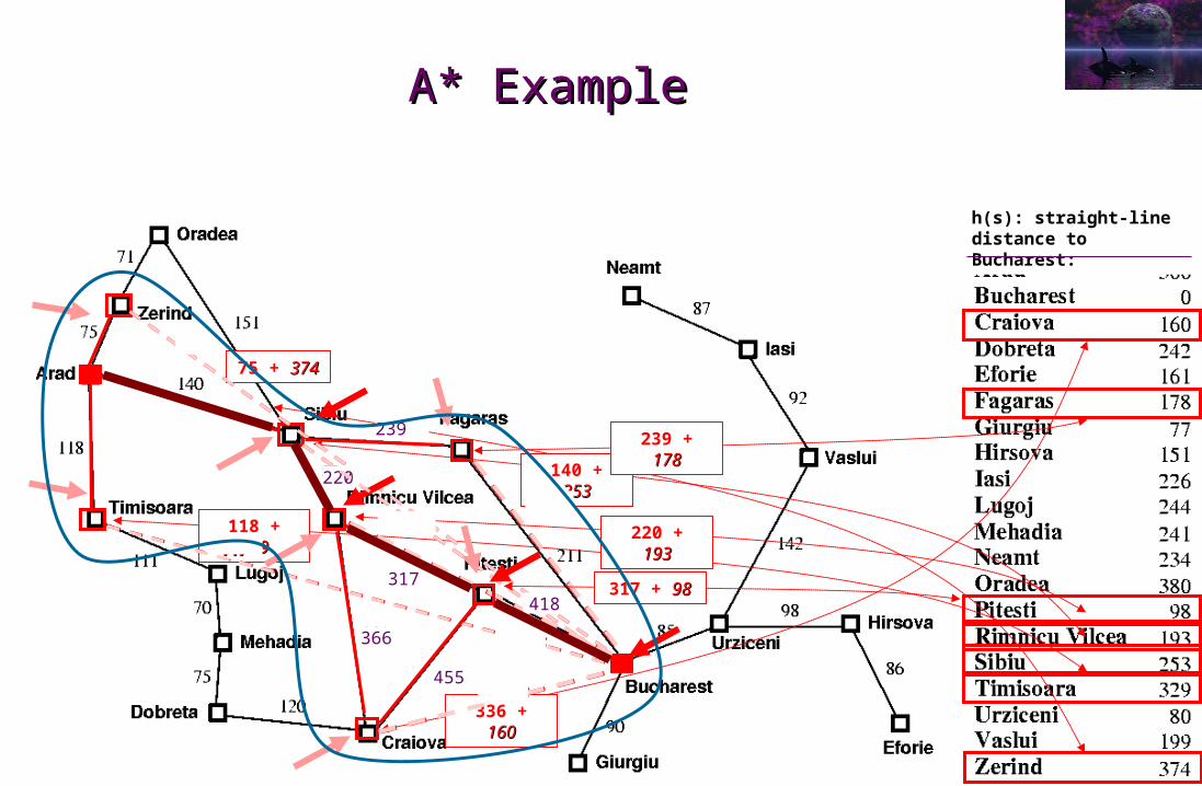
A* ExampleA* Example
h(s): straight-line distance to Bucharest:
75 + 374374449449
140 + 253253
393393118 + 329329447447
220
239239 + 178178
417417
220 + 193193
413413
366
317317 + 9898
415415
336 + 160160496496
455
418
A* Search CharacteristicsA* Search Characteristics
Strengths: Graph A* search is complete and Tree A* search is complete and optimal if h(s) is an
admissible heuristic, i.e., if it never overestimates the real cost to a goal Graph A* search if optimal if h(s) admissible and in addition a monotonic (or consistent)
heuristic h(s) is monotonic iff it satisfies the triangle inequality, i.e., s,s’ stateSpace (a actions, s’ = result(a,s)) h(s) cost(a) + h(s´)
A* is optimally efficient,i.e., no other optimal algorithm will expand fewer nodes than A* using the same heuristic function h(s)
Weakness: Runs out of memory for large problem instance because it keeps all generated nodes in
memory Why? Worst-case space complexity = O(bd), Unless n, |h(n) – c*(n)| O(log c*(n)) But very few practical heuristics verify this property
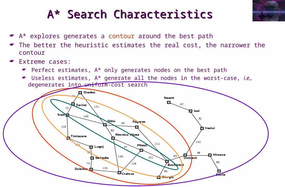
A* Search CharacteristicsA* Search Characteristics
A* explores generates a contour around the best path The better the heuristic estimates the real cost, the narrower the contour Extreme cases:
Perfect estimates, A* only generates nodes on the best path Useless estimates, A* generate all the nodes in the worst-case, i.e., degenerates into
uniform-cost search
Recursive Best-First Search (RBFS)Recursive Best-First Search (RBFS)
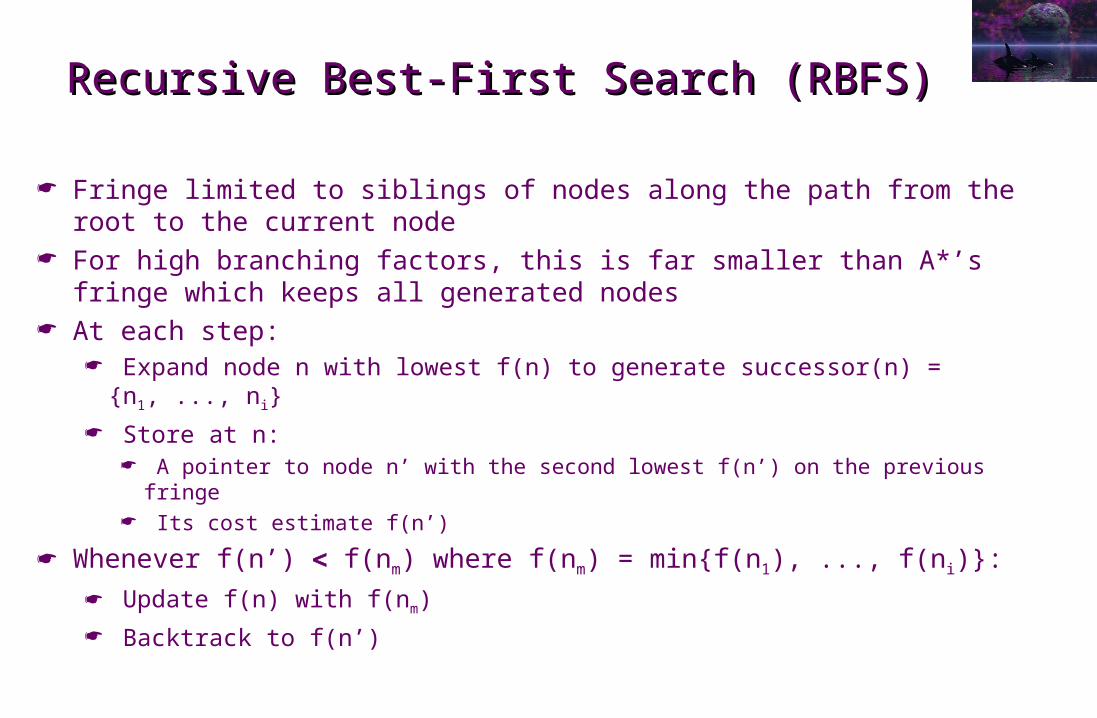
Fringe limited to siblings of nodes along the path from the root to the current node
For high branching factors, this is far smaller than A*’s fringe which keeps all generated nodes
At each step: Expand node n with lowest f(n) to generate successor(n) = {n1, ..., ni} Store at n:
A pointer to node n’ with the second lowest f(n’) on the previous fringe Its cost estimate f(n’)
Whenever f(n’) f(nm) where f(nm) = min{f(n1), ..., f(ni)}: Update f(n) with f(nm) Backtrack to f(n’)
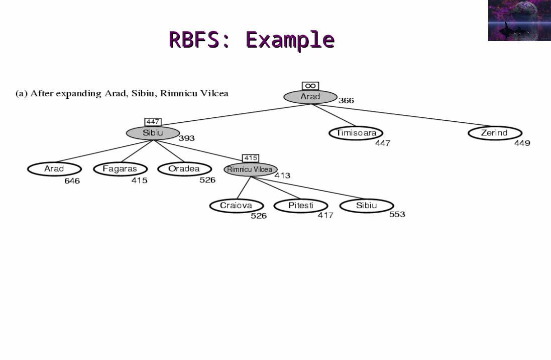
RBFS: ExampleRBFS: Example
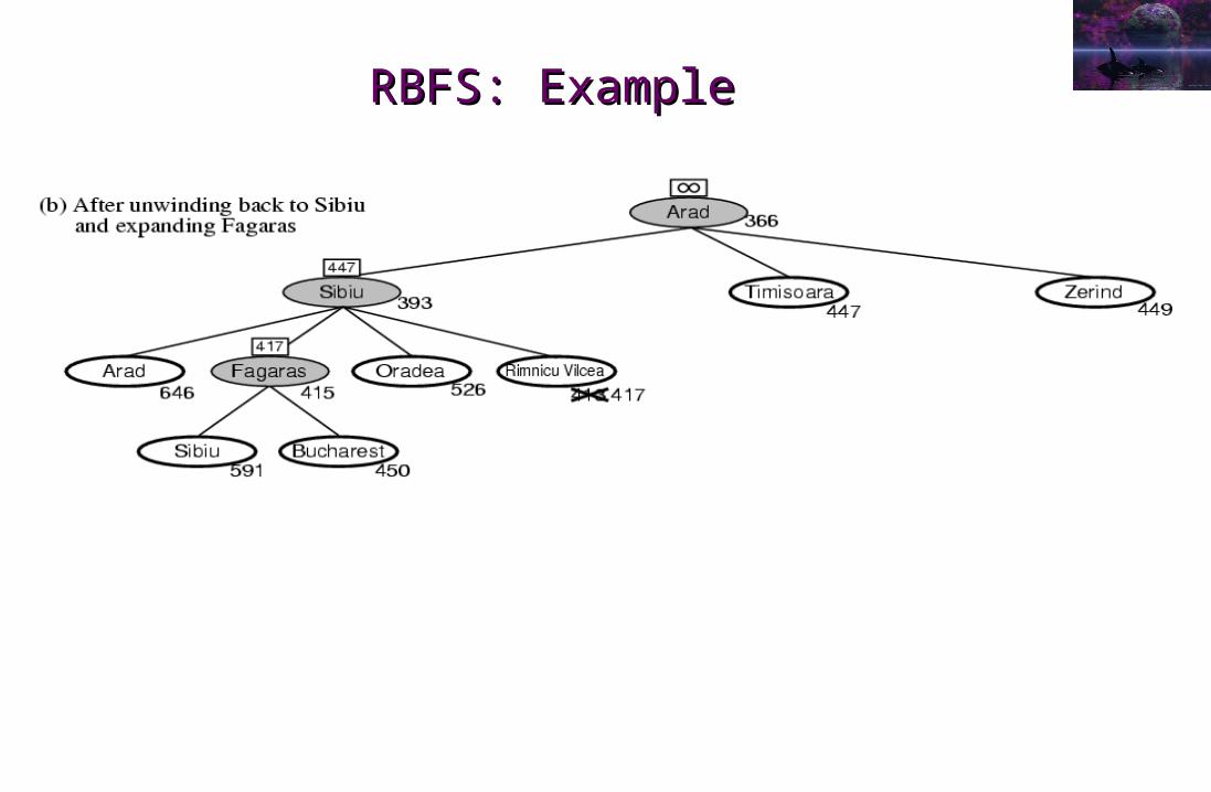
RBFS: ExampleRBFS: Example
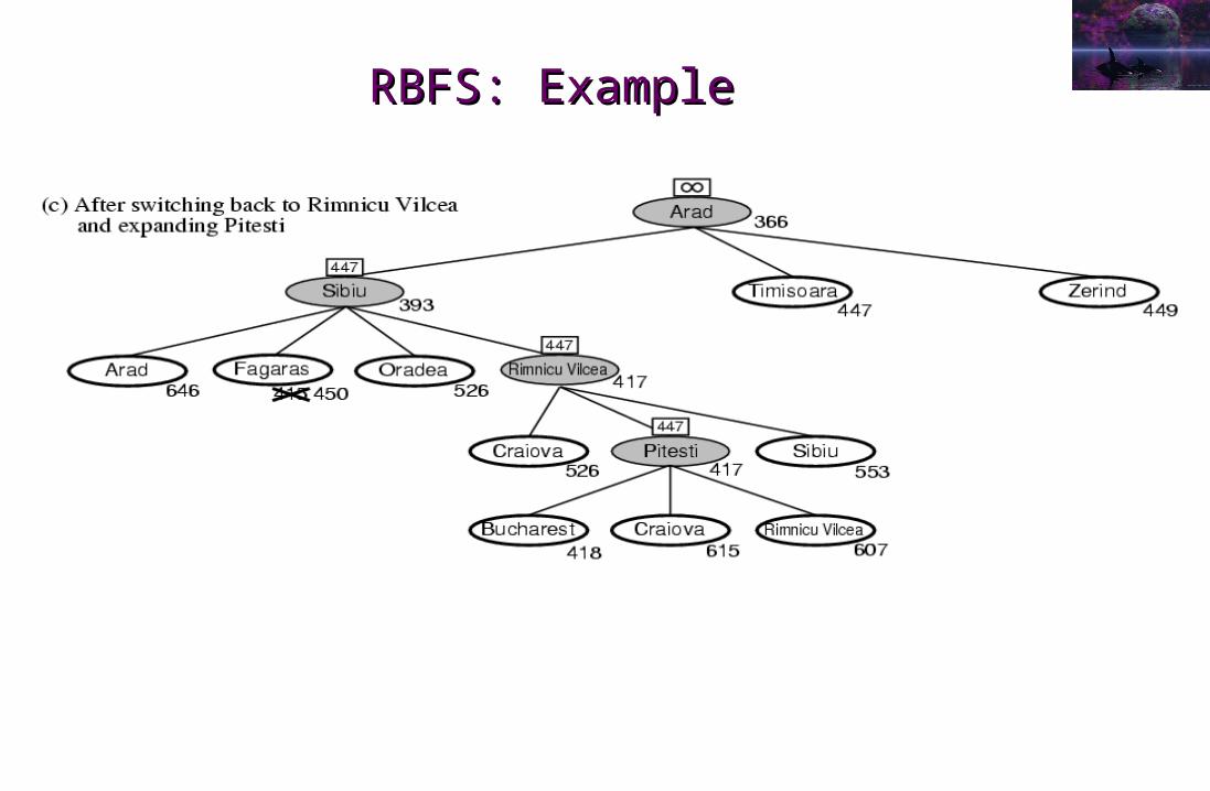
RBFS: ExampleRBFS: Example
RBFS: CharacteristicsRBFS: Characteristics
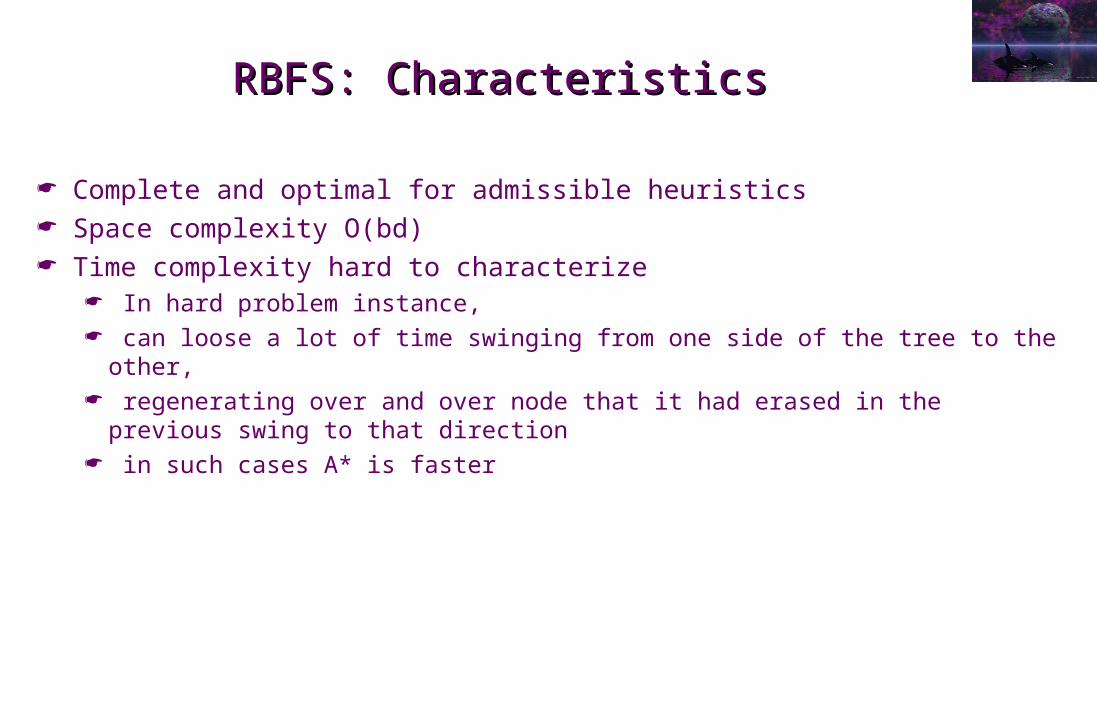
Complete and optimal for admissible heuristics Space complexity O(bd) Time complexity hard to characterize
In hard problem instance, can loose a lot of time swinging from one side of the tree to the other, regenerating over and over node that it had erased in the previous swing to
that direction in such cases A* is faster
Heuristic Function DesignHeuristic Function Design
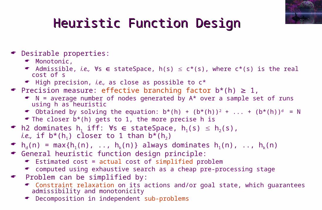
Desirable properties: Monotonic, Admissible, i.e., s stateSpace, h(s) c*(s), where c*(s) is the real cost of s High precision, i.e., as close as possible to c*
Precision measure: effective branching factor b*(h) 1, N = average number of nodes generated by A* over a sample set of runs using h as
heuristic Obtained by solving the equation: b*(h) + (b*(h))2 + ... + (b*(h))d = N The closer b*(h) gets to 1, the more precise h is
h2 dominates h1 iff: s stateSpace, h1(s) h2(s),i.e., if b*(h1) closer to 1 than b*(h2)
hd(n) = max{h1(n), .., hk(n)} always dominates h1(n), .., hk(n) General heuristic function design principle:
Estimated cost = actual cost of simplified problem computed using exhaustive search as a cheap pre-processing stage
Problem can be simplified by: Constraint relaxation on its actions and/or goal state, which guarantees admissibility
and monotonicity Decomposition in independent sub-problems
Heuristic Function Design: Heuristic Function Design: Constraint Relaxation ExampleConstraint Relaxation Example
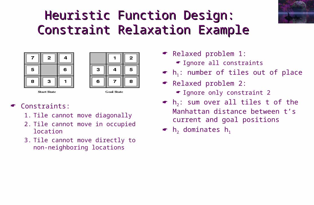
Constraints:1. Tile cannot move diagonally 2. Tile cannot move in occupied location3. Tile cannot move directly to non-
neighboring locations
Relaxed problem 1: Ignore all constraints
h1: number of tiles out of place Relaxed problem 2:
Ignore only constraint 2
h2: sum over all tiles t of the Manhattan distance between t’s current and goal positions
h2 dominates h1
Heuristic Function Design:Heuristic Function Design:Disjoint Pattern DatabasesDisjoint Pattern Databases
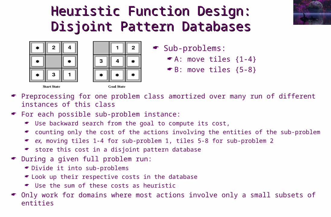
Preprocessing for one problem class amortized over many run of different instances of this class
For each possible sub-problem instance: Use backward search from the goal to compute its cost, counting only the cost of the actions involving the entities of the sub-problem ex, moving tiles 1-4 for sub-problem 1, tiles 5-8 for sub-problem 2 store this cost in a disjoint pattern database
During a given full problem run: Divide it into sub-problems Look up their respective costs in the database Use the sum of these costs as heuristic
Only work for domains where most actions involve only a small subsets of entities
Sub-problems: A: move tiles {1-4} B: move tiles {5-8}
Local Heuristic SearchLocal Heuristic Search
Search algorithms for complete state formulated problems for which the solution is only a target state that satisfies a goal or maximizes a utility function and not a path from the current initial state to that target state; ex:
Spatial equipment distribution (N-queens, VLSI, plant plan) Scheduling of vehicle assembly Task division among team members
Only keeps a very limited fringe in memory, often only the direct neighbors of the current node, or even only the current node. Far more scalable than global heuristic search, though generally neither complete nor optimal. Frequently used for multi-criteria optimization
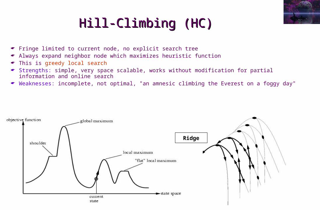
Ridge
Hill-Climbing (HC)Hill-Climbing (HC)
Fringe limited to current node, no explicit search tree Always expand neighbor node which maximizes heuristic function This is greedy local search Strengths: simple, very space scalable, works without modification for partial information and online
search Weaknesses: incomplete, not optimal, "an amnesic climbing the Everest on a foggy day"
Hill-Climbing VariationsHill-Climbing Variations
Stochastic HC: randomly chooses among uphill moves Slower convergence, but often better result
First-Choice HC: generates random successors instead of all successors of current node Efficient for state spaces with very high branching factor
HC with random restart to "pull out" from local maximum, plateau, ridges Simulated annealing:
Generates random moves Uphill moves always taken Downhill moves taken with a given probability that:
is lower for the steeper downhill moves decreases over time
Local SearchLocal Search
Key parameter of local search algorithms: Step size around current node (especially for real valued domains) Can also decrease over time during the search
Local beam search: Maintain a current fringe of k nodes Form the new fringe by expanding at once the k successors state with highest
utility from this entire fringe to form the new fringe Stochastic beam search:
At each step, pick successors semi-randomly with nodes with higher utility having a higher probability to be picked
It is a form of genetic search with asexual reproduction
In which Environments can a State Space In which Environments can a State Space Searching Agent (S3A) Act Successfully?Searching Agent (S3A) Act Successfully?
Fully observable? Partially observable? Sensorless? Deterministic or stochastic? Discrete or continuous? Episodic or non-episodic? Static? sequential? concurrent synchronous or concurrent asynchronous? Small or large? Lowly or highly diverse?
In which Environments can a State Space In which Environments can a State Space Searching Agent (S3A) Act Successfully?Searching Agent (S3A) Act Successfully?
Fully observable? Partially observable? Sensorless? An S3A can act successfully in an environment that is either partially observable
or even sensorless, provided that it is deterministic, small, lowly diverse and that the agent possesses an action model
Instead of searching in the space of states, it can search in the space of possible state sets (beliefs) to know which actions are potentially available
Deterministic or stochastic? An S3A can act successfully in an environment that is stochastic provided that it
is small and at least partially observable Instead of searching offline in the space of states, it can search offline in the
space of possible state sets (beliefs) resulting of an action with stochastic effects It can also search online and generate action programs or conditional plans
instead of mere action sequences, ex, [suck, right, {if right.dirty then suck}] Discrete or continuous?
An S3A using a global search algorithm can only act successfully in an discrete environment, for continuous variables imply infinite branching factor
In which Environments can a State Space In which Environments can a State Space Searching Agent (S3A) Act Successfully?Searching Agent (S3A) Act Successfully?
Episodic or non-episodic? An S3A is only necessary for a non-episodic environment which requires
choosing action sequences, where the choice of one action conditions the action range subsequently available
Static? sequential? concurrent synchronous or concurrent asynchronous? An S3A can only act successfully in a static or sequential environment, for
there is no point in searching for goal-achieving or optimal action sequences in an environment that changes due to factors outside the control of the agent
Small or large? An S3A can only act successfully in a medium-sized environment provided
that it is deterministic and at least partially observable, or small environment that are either stochastic or sensorless
Lowly or highly diverse? An S3A can only act successfully in low diversity environment for diversity
affects directly the branching factor of the problem search tree space

Searching in the Space of Possible State Searching in the Space of Possible State SetsSets
Top Related