


Languages
Pages
Legal


On the ?-Sylvester Equation AX ± X ?B? = C
Chun-Yueh Chiang
Department of Applied MathematicsNational Chiao Tung University, Taiwan
A joint work with E. K.-W. Chu and W.-W. Lin
Oct., 20, 2008
Chun-Yueh Chiang On the ?-Sylvester Equation AX ± X?B? = C

Introduction ?-Sylvester Equation Numerical Examples Related Equations Conclusions
Outline
1 Introduction
2 ?-Sylvester Equation
3 Numerical Examples
4 Related Equations
5 Conclusions
Chun-Yueh Chiang On the ?-Sylvester Equation AX ± X?B? = C

Introduction ?-Sylvester Equation Numerical Examples Related Equations Conclusions
Outline
1 Introduction
2 ?-Sylvester Equation
3 Numerical Examples
4 Related Equations
5 Conclusions
Chun-Yueh Chiang On the ?-Sylvester Equation AX ± X?B? = C
Introduction ?-Sylvester Equation Numerical Examples Related Equations Conclusions
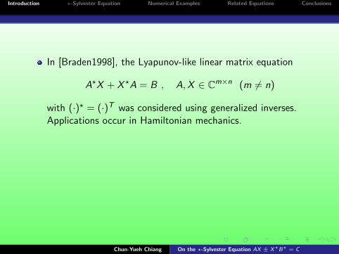
In [Braden1998], the Lyapunov-like linear matrix equation
A?X + X ?A = B , A,X ∈ Cm×n (m 6= n)
with (·)? = (·)T was considered using generalized inverses.Applications occur in Hamiltonian mechanics.
In this talk, we consider the ?-Sylvester equation
AX ± X ?B? = C , A,B,X ∈ Cn×n. (1.1)
This includes the special cases of the T-Sylvester equationwhen ? = T and the H-Sylvester equation when ? = H.
Chun-Yueh Chiang On the ?-Sylvester Equation AX ± X?B? = C

Introduction ?-Sylvester Equation Numerical Examples Related Equations Conclusions
Some related equations of (1.1), e.g., AXB? ± X ? = C ,AXB? ± CX ?D? = E , AX ± X ?A? = C , AX ± YB = C ,AXB ± CYD = E , AXA? ± BYB? = C andAXB ± (AXB)? = C will also be studied.
Our tools include the (generalized and periodic) Schur,(generalized) singular value and QR decompositions.
An interesting application, for the ?-Sylvester equation (1.1)
AX ± X ?B? = C , A,B,X ∈ Cn×n
arises from the eigensolution of the palindromic linearization[Chu2007]
Chun-Yueh Chiang On the ?-Sylvester Equation AX ± X?B? = C
Introduction ?-Sylvester Equation Numerical Examples Related Equations Conclusions
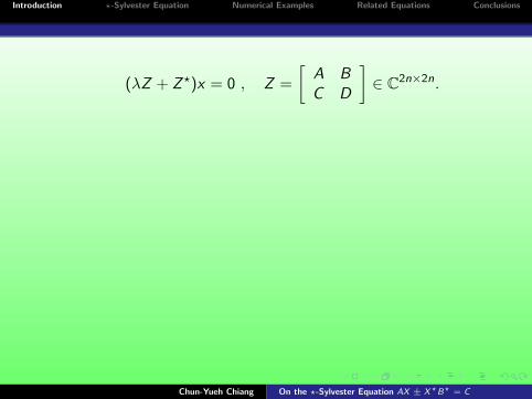
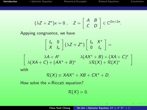
(λZ + Z ?)x = 0 , Z =
[A BC D
]∈ C2n×2n.
Appying congruence, we have[In 0X In
](λZ + Z ?)
[In X ?
0 In
]=
[λA + A? λ(AX ? + B) + (XA + C )?
λ(XA + C ) + (AX ? + B)? λR(X ) +R(X )∗
]with
R(X ) ≡ XAX ? + XB + CX ? + D.
How solve the ?-Riccati equation?
R(X ) = 0.
Chun-Yueh Chiang On the ?-Sylvester Equation AX ± X?B? = C

Introduction ?-Sylvester Equation Numerical Examples Related Equations Conclusions
(λZ + Z ?)x = 0 , Z =
[A BC D
]∈ C2n×2n.
Appying congruence, we have[In 0X In
](λZ + Z ?)
[In X ?
0 In
]=
[λA + A? λ(AX ? + B) + (XA + C )?
λ(XA + C ) + (AX ? + B)? λR(X ) +R(X )∗
]with
R(X ) ≡ XAX ? + XB + CX ? + D.
How solve the ?-Riccati equation?
R(X ) = 0.
Chun-Yueh Chiang On the ?-Sylvester Equation AX ± X?B? = C

Introduction ?-Sylvester Equation Numerical Examples Related Equations Conclusions
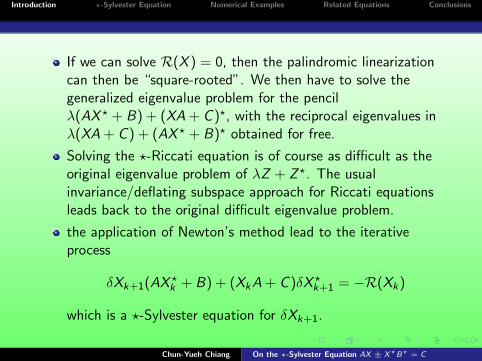
If we can solve R(X ) = 0, then the palindromic linearizationcan then be “square-rooted”. We then have to solve thegeneralized eigenvalue problem for the pencilλ(AX ? + B) + (XA + C )?, with the reciprocal eigenvalues inλ(XA + C ) + (AX ? + B)? obtained for free.
Solving the ?-Riccati equation is of course as difficult as theoriginal eigenvalue problem of λZ + Z ?. The usualinvariance/deflating subspace approach for Riccati equationsleads back to the original difficult eigenvalue problem.
the application of Newton’s method lead to the iterativeprocess
δXk+1(AX ?k + B) + (XkA + C )δX ?
k+1 = −R(Xk)
which is a ?-Sylvester equation for δXk+1.
Chun-Yueh Chiang On the ?-Sylvester Equation AX ± X?B? = C

Introduction ?-Sylvester Equation Numerical Examples Related Equations Conclusions
If we can solve R(X ) = 0, then the palindromic linearizationcan then be “square-rooted”. We then have to solve thegeneralized eigenvalue problem for the pencilλ(AX ? + B) + (XA + C )?, with the reciprocal eigenvalues inλ(XA + C ) + (AX ? + B)? obtained for free.
Solving the ?-Riccati equation is of course as difficult as theoriginal eigenvalue problem of λZ + Z ?. The usualinvariance/deflating subspace approach for Riccati equationsleads back to the original difficult eigenvalue problem.
the application of Newton’s method lead to the iterativeprocess
δXk+1(AX ?k + B) + (XkA + C )δX ?
k+1 = −R(Xk)
which is a ?-Sylvester equation for δXk+1.
Chun-Yueh Chiang On the ?-Sylvester Equation AX ± X?B? = C

Introduction ?-Sylvester Equation Numerical Examples Related Equations Conclusions
Outline
1 Introduction
2 ?-Sylvester Equation
3 Numerical Examples
4 Related Equations
5 Conclusions
Chun-Yueh Chiang On the ?-Sylvester Equation AX ± X?B? = C

Introduction ?-Sylvester Equation Numerical Examples Related Equations Conclusions
Recalled the ?-Sylvester equation (1.1)
AX ± X ?B? = C , A,B,X ∈ Cn×n.
With the Kronecker product, (1.1) can be written as
P vec(X ) = vec(C ) , P ≡ I ⊗ A± (B ⊗ I )E , (2.1)
where
A⊗ B ≡ [aijB] ∈ Cn2×n2, vec(X ) ≡
X (:, 1)X (:, 2)
...X (:, n)
∈ Cn2×1.
Chun-Yueh Chiang On the ?-Sylvester Equation AX ± X?B? = C
Introduction ?-Sylvester Equation Numerical Examples Related Equations Conclusions
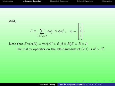
And,
E ≡∑
1≤i ,j≤n
eie>j ⊗ eje
>i , ei =
...1...
.Note that E vec(X ) = vec(XT ), E (A⊗ B)E = B ⊗ A.
The matrix operator on the left-hand-side of (2.1) is n2 × n2.
The application of Gaussian elimination and the like will beinefficient.
The approach ignores the structure of the original problem.
Chun-Yueh Chiang On the ?-Sylvester Equation AX ± X?B? = C

Introduction ?-Sylvester Equation Numerical Examples Related Equations Conclusions
And,
E ≡∑
1≤i ,j≤n
eie>j ⊗ eje
>i , ei =
...1...
.Note that E vec(X ) = vec(XT ), E (A⊗ B)E = B ⊗ A.
The matrix operator on the left-hand-side of (2.1) is n2 × n2.
The application of Gaussian elimination and the like will beinefficient.
The approach ignores the structure of the original problem.
Chun-Yueh Chiang On the ?-Sylvester Equation AX ± X?B? = C
Introduction ?-Sylvester Equation Numerical Examples Related Equations Conclusions
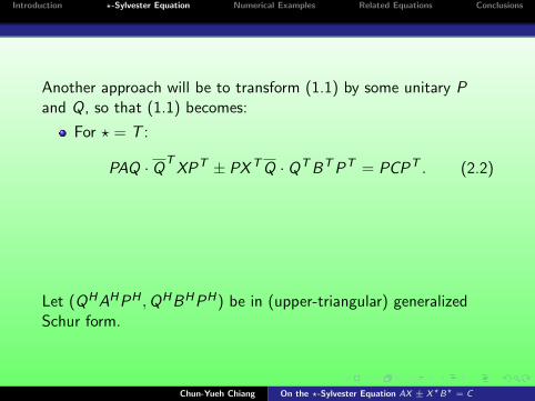
Another approach will be to transform (1.1) by some unitary Pand Q, so that (1.1) becomes:
For ? = T :
PAQ · QTXPT ± PXTQ · QTBTPT = PCPT . (2.2)
For ? = H:
PAQ · QHXPH ± PXHQ · QHBHPH = PCPH . (2.3)
Let (QHAHPH ,QHBHPH) be in (upper-triangular) generalizedSchur form.
Chun-Yueh Chiang On the ?-Sylvester Equation AX ± X?B? = C

Introduction ?-Sylvester Equation Numerical Examples Related Equations Conclusions
The transformed equations in (2.2) and (2.3) then have the form[a11 0T
a21 A22
] [x11 x?12
x21 X22
]±[
x?11 x?21
x12 X ?22
] [b?11 b?21
0 B?22
](2.4)
=
[c11 c?12
c21 C22
].
Multiply the matrices out, we have
Chun-Yueh Chiang On the ?-Sylvester Equation AX ± X?B? = C

Introduction ?-Sylvester Equation Numerical Examples Related Equations Conclusions
a11x11 ± b?11x?11 = c11, (2.5)
a11x?12 ± x?21B
?22 = c?12 ∓ x?11b
?21, (2.6)
A22x21 ± b?11x12 = c21 − x11a21, (2.7)
A22X22 ± X ?22B
?22 = C22 ≡ C22 − a21x
?12 ∓ x12b
?21.(2.8)
From (2.5) for ? = T , we have
(a11 ± b11)x11 = c11. (2.9)
Let λ1 ≡ a11/b11 ∈ σ(A,B). The solvability condition of theabove equation is
a11 ± b11 6= 0⇔ λ1 6= ∓1. (2.10)
Chun-Yueh Chiang On the ?-Sylvester Equation AX ± X?B? = C

Introduction ?-Sylvester Equation Numerical Examples Related Equations Conclusions
From (2.5) when ? = H, we have
a11x11 ± b11x11 = c11. (2.11)
To solve (2.11) is to write it together with its complexconjugate in the composite form[
a11 ±b?11
±b11 a?11
] [x11
x?11
]=
[c11
c?11
].
The determinant of the matrix operator in above:
d = |a11|2 − |b11|2 6= 0⇔ |λ11| 6= 1. (2.12)
requiring that no eigenvalue λ ∈ σ(A,B) lies on the unitcircle.
Chun-Yueh Chiang On the ?-Sylvester Equation AX ± X?B? = C

Introduction ?-Sylvester Equation Numerical Examples Related Equations Conclusions
From (2.6) and (2.7), we obtain[a?11I ±B22
±b?11I A22
] [x12
x21
]=
[c12
c21
]≡[
c12
c21
]+ x11
[∓b21
−a21
].
(2.13)With a11 = b11 = 0, x11 will be undetermined. However,σ(A,B) = C and this case will be excluded by (2.16).
If a11 6= 0, (2.13) is then equivalent to[a?11I ±B22
0 A22 −b?
11a?11
B22
][x12
x21
]=
[c12
c21
]≡
[c12
c21 ∓b?
11a?11
c12
].
(2.14)The solvability condition of (2.13) and (2.14) is
det A22 6= 0 , A22 ≡ A22 −b?11
a?11
B22
or that λ and λ−? cannot be in σ(A,B) together. Note thatA22 is still lower-triangular, just like A or B.
Chun-Yueh Chiang On the ?-Sylvester Equation AX ± X?B? = C

Introduction ?-Sylvester Equation Numerical Examples Related Equations Conclusions
If b11 6= 0, (2.13) is equivalent to[0 B22 −
a?11
b?11
A22
b?11I ±A22
] [x12
x21
]=
[c12
±c21
]≡
[±c12 −
a?11
b?11
c21
±c21
](2.15)
with an identical solvability condition (2.16). Lastly, (2.8) isof the same form as (1.1) but of smaller size.
We summarize the solvability condition for (1.1) in the followingtheorem:
Theorem1
The ?-Sylvester equation (1.1):
AX ± X ?B? = C , A,B ∈ Cn×n
is uniquely solvable if and only if the condition:
Chun-Yueh Chiang On the ?-Sylvester Equation AX ± X?B? = C

Introduction ?-Sylvester Equation Numerical Examples Related Equations Conclusions
λ ∈ σ(A,B)⇒ λ−? 6∈ σ(A,B) (2.16)
is satisfied. Here, the convention that 0 and ∞ are mutuallyreciprocal is followed.
The process in this subsection is summarized below: (with BSdenoting back-substitution)
Algorithm SSylvester
(For the unique solution of AX ± X ?B? = C ; A,B,C ,X ∈ Cn×n.)
Compute the lower-triangular generalized Schur form(PAQ,PBQ) using QZ.
Store (PAQ,PBQ,PCP∗) in (A,B,C ).
Solve (2.9) for ? = T , or (2.11) for ? = H; if fail, exit.
Chun-Yueh Chiang On the ?-Sylvester Equation AX ± X?B? = C

Introduction ?-Sylvester Equation Numerical Examples Related Equations Conclusions
If n = 1 or |a11|2 + |b11|2 ≤ tolerance, exit.If |a11| ≥ |b11|, thenif A22 ≡ A22 −
b?11
a?11
B22 has any negligible diagonal elements,then exit.Else if B22 ≡ B22 −
a?11
b?11
A22 has any negligible diagonal elements,then exit.Else compute x21 = B−1
22 c12 by BS, x12 = (±c21 ∓ A22x21) /b?11
(c.f. (2.15)).
Apply Algorithm TSylvester to A22X22 ± X ?22B
?22 = C22,
n← n − 1.
Output X ← QXP for ? = T , or X ← QXP for ? = H.
End of algorithm
Chun-Yueh Chiang On the ?-Sylvester Equation AX ± X?B? = C

Introduction ?-Sylvester Equation Numerical Examples Related Equations Conclusions
Cost
Let the operation count of the Algorithm SSylvester be f (n)complex flops, we assume that A, B are lower-triangular matrices.(After a QZ procedure (66n3))
Inverting A22 ≡ A22 −b?
11a?11
B22 or B22 ≡ B22 −a?11
b?11
A22 (12n2
flops).
Computing x21 = B−122 c12 and x12 = (±c21 ∓ A22x21) /b?11 (n2
flops).
Forming C22 = C22 − a21x?12 ∓ x12a
?21 (2n2).
Thus f (n) ≈ f (n − 1) + 72n2, ignoring O(n) terms. This implies
that f (n) ≈ 76n3 and the total operation count for
Algorithm SSylvester is 6716n3 complex flops, ignoring O(n2) terms.
Chun-Yueh Chiang On the ?-Sylvester Equation AX ± X?B? = C

Introduction ?-Sylvester Equation Numerical Examples Related Equations Conclusions
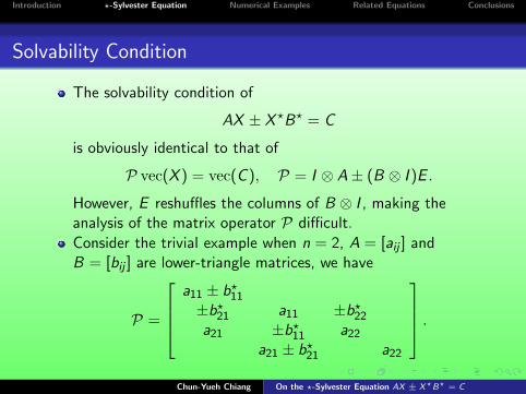
Solvability Condition
The solvability condition of
AX ± X ?B? = C
is obviously identical to that of
P vec(X ) = vec(C ), P = I ⊗ A± (B ⊗ I )E .
However, E reshuffles the columns of B ⊗ I , making theanalysis of the matrix operator P difficult.
Consider the trivial example when n = 2, A = [aij ] andB = [bij ] are lower-triangle matrices, we have
P =
a11 ± b?11
±b?21 a11 ±b?22
a21 ±b?11 a22
a21 ± b?21 a22
.
Chun-Yueh Chiang On the ?-Sylvester Equation AX ± X?B? = C
Introduction ?-Sylvester Equation Numerical Examples Related Equations Conclusions
Solvability Condition
The solvability condition of
AX ± X ?B? = C
is obviously identical to that of
P vec(X ) = vec(C ), P = I ⊗ A± (B ⊗ I )E .
However, E reshuffles the columns of B ⊗ I , making theanalysis of the matrix operator P difficult.
Consider the trivial example when n = 2, A = [aij ] andB = [bij ] are lower-triangle matrices, we have
P =
a11 ± b?11
±b?21 a11 ±b?22
a21 ±b?11 a22
a21 ± b?21 a22
.Chun-Yueh Chiang On the ?-Sylvester Equation AX ± X?B? = C
Introduction ?-Sylvester Equation Numerical Examples Related Equations Conclusions
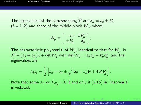
The eigenvalues of the corresponding P are λii = aii ± b?ii(i = 1, 2) and those of the middle block W12 where
Wij ≡[
aii ±b?jj±b?ii ajj
].
The characteristic polynomial of Wij , identical to that for Wji , isλ2 − (aii + ajj)λ+ det Wij with det Wij = aiiajj − b?iib
?jj , and the
eigenvalues are
λWij=
1
2
[aii + ajj ±
√(aii − ajj)2 + 4b?iib
?jj
].
Note that some λii or λWij= 0 if and only if (2.16) in Theorem 1
is violated.
Chun-Yueh Chiang On the ?-Sylvester Equation AX ± X?B? = C

Introduction ?-Sylvester Equation Numerical Examples Related Equations Conclusions
Outline
1 Introduction
2 ?-Sylvester Equation
3 Numerical Examples
4 Related Equations
5 Conclusions
Chun-Yueh Chiang On the ?-Sylvester Equation AX ± X?B? = C
Introduction ?-Sylvester Equation Numerical Examples Related Equations Conclusions
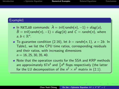
Example1
In MATLAB commands: A = tril(randn(n),−1) + diag(a),B = tril(randn(n),−1) + diag(b) and C = randn(n), wherea, b ∈ Rn.
To guarantee condition (2.16), let b = randn(n, 1), a = 2b. InTable1, we list the CPU time ratios, corresponding residualsand their ratios, with increasing dimensionsn = 16, 25, 30, 35, 40.
Note that the operation counts for the SSA and KRP methodsare approximately 67n3 and 2
3n6 flops respectively (the latterfor the LU decomposition of the n2 × n2 matrix in (2.1).
Chun-Yueh Chiang On the ?-Sylvester Equation AX ± X?B? = C

Introduction ?-Sylvester Equation Numerical Examples Related Equations Conclusions
Table1: Results for Example1
n tKRPtASS
Res(ASS) Res(KRP) Res(KRP)Res(ASS)
16 1.00e+00 1.8527e-17 2.1490e-17 1.1625 1.31e+01 2.3065e-17 2.8686e-17 1.2430 2.61e+01 3.1126e-18 5.7367e-18 2.2035 6.48e+01 7.0992e-18 1.2392e-17 1.7540 1.05e+02 1.7654e-18 6.4930e-18 3.68
Chun-Yueh Chiang On the ?-Sylvester Equation AX ± X?B? = C
Introduction ?-Sylvester Equation Numerical Examples Related Equations Conclusions
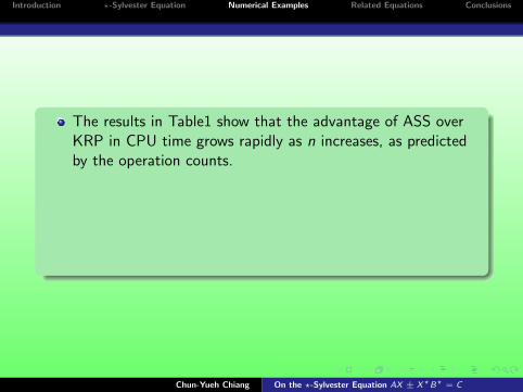
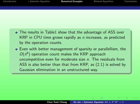
The results in Table1 show that the advantage of ASS overKRP in CPU time grows rapidly as n increases, as predictedby the operation counts.
Even with better management of sparsity or parallellism, theO(n6) operation count makes the KRP approachuncompetitive even for moderate size n. The residuals fromASS is also better than that from KRP, as (2.1) is solved byGaussian elimination in an unstructured way.
Chun-Yueh Chiang On the ?-Sylvester Equation AX ± X?B? = C
Introduction ?-Sylvester Equation Numerical Examples Related Equations Conclusions
The results in Table1 show that the advantage of ASS overKRP in CPU time grows rapidly as n increases, as predictedby the operation counts.
Even with better management of sparsity or parallellism, theO(n6) operation count makes the KRP approachuncompetitive even for moderate size n. The residuals fromASS is also better than that from KRP, as (2.1) is solved byGaussian elimination in an unstructured way.
Chun-Yueh Chiang On the ?-Sylvester Equation AX ± X?B? = C

Introduction ?-Sylvester Equation Numerical Examples Related Equations Conclusions
Example2
We let a = [α + ε, β]>, b = [β, α]>, where α, β are tworandomly numbers greater than 1, with the spectral setσ(A,B) = {α+ε
β , βα}, and |λ1λ2 − 1| = εα . Judging from
(2.16), (1.1) has worsening condition when ε decreases.
We report a comparison of absolute residuals for the ASS andKRP approaches for ε = 10−1, 10−3, 10−5, 10−7 and 10−9 inTable2.
The results show that if (2.1) is solved by Guassianelimination, its residual will be larger than that for ASSespecially for smaller ε. Note that the size of X reflectspartially the condition of (1.1). The KRP approach copes lesswell than the ASS approach for an ill-conditioned problem.
Chun-Yueh Chiang On the ?-Sylvester Equation AX ± X?B? = C

Introduction ?-Sylvester Equation Numerical Examples Related Equations Conclusions
Table2: Results for Example2
ε Res(ASS) Res(KRP) Res(KRP)Res(ASS) O(‖X‖)
1.0e-1 2.0673e-15 2.4547e-15 1.19 101
1.0e-3 8.6726e-13 4.3279e-13 0.50 103
1.0e-5 2.3447e-12 2.4063e-12 1.03 103
1.0e-7 5.9628e-10 1.1786e-09 1.98 106
1.0e-9 5.8632e-08 3.4069e-07 5.81 108
Chun-Yueh Chiang On the ?-Sylvester Equation AX ± X?B? = C

Introduction ?-Sylvester Equation Numerical Examples Related Equations Conclusions
Outline
1 Introduction
2 ?-Sylvester Equation
3 Numerical Examples
4 Related Equations
5 Conclusions
Chun-Yueh Chiang On the ?-Sylvester Equation AX ± X?B? = C

Introduction ?-Sylvester Equation Numerical Examples Related Equations Conclusions
Generalized ?-Sylvester equation I
The more general version of the ?-Sylvester equation I:
AXB? ± X ? = C
with A,B?,X ? ∈ Cm×n is uniquely solvable if and only if thecondition:
λ ∈ σ(AB)⇒ λ−? 6∈ σ(AB)
is satisfied.
Chun-Yueh Chiang On the ?-Sylvester Equation AX ± X?B? = C
Introduction ?-Sylvester Equation Numerical Examples Related Equations Conclusions
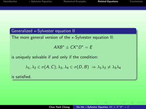
Generalized ?-Sylvester equation II
The more general version of the ?-Sylvester equation II:
AXB? ± CX ?D? = E
is uniquely solvable if and only if the condition:
λ1, λ2 ∈ σ(A,C );λ3, λ4 ∈ σ(D,B) ⇒ λ1λ2 6= λ3λ4
is satisfied.
Chun-Yueh Chiang On the ?-Sylvester Equation AX ± X?B? = C

Introduction ?-Sylvester Equation Numerical Examples Related Equations Conclusions
Outline
1 Introduction
2 ?-Sylvester Equation
3 Numerical Examples
4 Related Equations
5 Conclusions
Chun-Yueh Chiang On the ?-Sylvester Equation AX ± X?B? = C

Introduction ?-Sylvester Equation Numerical Examples Related Equations Conclusions
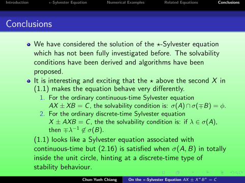
Conclusions
We have considered the solution of the ?-Sylvester equationwhich has not been fully investigated before. The solvabilityconditions have been derived and algorithms have beenproposed.
It is interesting and exciting that the ? above the second X in(1.1) makes the equation behave very differently.
1. For the ordinary continuous-time Sylvester equationAX ±XB = C , the solvability condition is: σ(A)∩σ(∓B) = φ.
2. For the ordinary discrete-time Sylvester equationX ± AXB = C , the the solvability condition is: if λ ∈ σ(A),then ∓λ−1 6∈ σ(B).
(1.1) looks like a Sylvester equation associated withcontinuous-time but (2.16) is satisfied when σ(A,B) in totallyinside the unit circle, hinting at a discrete-time type ofstability behaviour.
Chun-Yueh Chiang On the ?-Sylvester Equation AX ± X?B? = C
Introduction ?-Sylvester Equation Numerical Examples Related Equations Conclusions
Conclusions
We have considered the solution of the ?-Sylvester equationwhich has not been fully investigated before. The solvabilityconditions have been derived and algorithms have beenproposed.It is interesting and exciting that the ? above the second X in(1.1) makes the equation behave very differently.
1. For the ordinary continuous-time Sylvester equationAX ±XB = C , the solvability condition is: σ(A)∩σ(∓B) = φ.
2. For the ordinary discrete-time Sylvester equationX ± AXB = C , the the solvability condition is: if λ ∈ σ(A),then ∓λ−1 6∈ σ(B).
(1.1) looks like a Sylvester equation associated withcontinuous-time but (2.16) is satisfied when σ(A,B) in totallyinside the unit circle, hinting at a discrete-time type ofstability behaviour.
Chun-Yueh Chiang On the ?-Sylvester Equation AX ± X?B? = C

Introduction ?-Sylvester Equation Numerical Examples Related Equations Conclusions
Thank you for your attention!
Chun-Yueh Chiang On the ?-Sylvester Equation AX ± X?B? = C
Top Related