
![NERC - Electric Reliability Council of Texas this page%PDF-1.5 %âãÏÓ 6553 0 obj > endobj 6570 0 obj >/Filter/FlateDecode/ID[5CBE1A85C88D924BB6FDDCE8566271B5>65EFB89FDA6EAB4BB03D5724D09DF92B>]/Index[6553](https://static.fdocuments.in/doc/165x107/5aaafda17f8b9aa9488b6c06/nerc-electric-reliability-council-of-this-pagepdf-15-6553-0-obj-endobj-6570.jpg)


Languages
Pages
Legal


Examensarbete vid Institutionen för geovetenskaper ISSN 1650-6553 Nr 286
On the Relation Between Arctic Sea Ice and European
Cold Winters During the Little Ice Age 1400-1850
On the Relation Between Arctic Sea Ice and European Cold Winters During the Little Ice Age 1400-1850
Kristian Silver
Kristian Silver
This study aims to investigate the possible historical correlation between sea ice reduction in the Arctic and cold winters in Central Europe. The study is conducted over a cold period in Europe known as the Little Ice Age (LIA), 1400–1850, and uses a Global Climate Model with eight different forcing scenarios. Temperature data from Central Europe and ice data from the Arctic are extracted from the model and compared. The assumed relationship has been presented in various forms in the last few years. Essentially, it is argued that less sea ice in a particular area in the Arctic (around the Barents and Kara Seas) could affect large-scale atmospheric circulation patterns, including the North Atlantic oscillation (NAO), and then give rise to cold European winters. Thus, this essay also recreates the NAO over the same historical period. The results of this study are not, however, able to confirm this theory; over longer periods the identified correlation is rather the opposite. It is speculated that this mechanism could include a threshold, where it might not be noticeable for historical, heavier ice-conditions; but more so for future, global warming scenarios. However, a correlation tendency is identified in some of the model runs, suggesting that a feedback effect such as this, if it existed, might be more likely to affect temperatures of individual months rather than the entire winter. A very weak response is also found for the NAO itself. The model’s suitability for this kind of study is then discussed. Although it might not precisely capture each type of year-to-year comparison used in this study, it is proven to have some response to known individual events in climatological history. Finally, it is concluded that this study alone cannot disprove the proposed theory, and that further investigation is required.
Uppsala universitet, Institutionen för geovetenskaperExamensarbete E i Meteorologi, 30 hp ISSN 1650-6553 Nr 286Tryckt hos Institutionen för geovetenskaper, Geotryckeriet, Uppsala universitet, Uppsala, 2014.

Supervisor: Hans Bergström
Examensarbete vid Institutionen för geovetenskaper ISSN 1650-6553 Nr 286
On the Relation Between Arctic Sea Ice and European
Cold Winters During the Little Ice Age 1400-1850
Kristian Silver

Copyright © and the Department of Earth Sciences Uppsala UniversityPublished at Department of Earth Sciences, Geotryckeriet Uppsala University, Uppsala, 2014

3
Abstract
This study aims to investigate the possible historical correlation between sea ice reduction
in the Arctic and cold winters in Central Europe. The study is conducted over a cold period
in Europe known as the Little Ice Age (LIA), 1400–1850, and uses a Global Climate Model
with eight different forcing scenarios. Temperature data from Central Europe and ice data
from the Arctic are extracted from the model and compared. The assumed relationship has
been presented in various forms in the last few years. Essentially, it is argued that less sea
ice in a particular area in the Arctic (around the Barents and Kara Seas) could affect large-
scale atmospheric circulation patterns, including the North Atlantic oscillation (NAO), and
then give rise to cold European winters. Thus, this essay also recreates the NAO over the
same historical period. The results of this study are not, however, able to confirm this
theory; over longer periods the identified correlation is rather the opposite. It is
speculated that this mechanism could include a threshold, where it might not be
noticeable for historical, heavier ice-conditions; but more so for future, global warming
scenarios. However, a correlation tendency is identified in some of the model runs,
suggesting that a feedback effect such as this, if it existed, might be more likely to affect
temperatures of individual months rather than the entire winter. A very weak response is
also found for the NAO itself. The model’s suitability for this kind of study is then
discussed. Although it might not precisely capture each type of year-to-year comparison
used in this study, it is proven to have some response to known individual events in
climatological history. Finally, it is concluded that this study alone cannot disprove the
proposed theory, and that further investigation is required.
Keywords: Barents Sea, Kara Sea, sea ice reduction, Arctic, midlatitudes, feedback effect,
Last Millennium, historical climate change, climate modeling, threshold, global warming,
cold winters, Little Ice Age, North Atlantic oscillation, LIA, NAO, PMIP3, CMIP5, NASA-GISS.

4

5
Referat (summary in Swedish)
Denna studie syftar till att undersöka en möjlig historisk koppling mellan minskad havsis i
Arktis och kalla vintrar i Centraleuropa. Studien undersöker en lång kallperiod i Europa,
"Lilla istiden", som ägde rum ungefär mellan 1400 och 1850. En global klimatmodell med
åtta olika drivningsscenarier används, och både temperatur- och isdata extraheras från
denna och jämförs. Teorin som studien bygger på har lagts fram i varierande former under
de senaste åren, men i stort argumenterar den för att ett minskat istäcke i ett område i
Arktis, nämligen Barents- och Karahavet, kan påverka större cirkulationsmönster i
atmosfären. Detta inkluderar även den Nordatlantiska oscillationen (NAO), vilket kan ge
upphov till kalla vintrar i Europa. Denna studie återskapar därför is- och
temperaturförhållandena för det ovan nämndaområdet i Arktis, samt även NAO under den
aktuella historiska tidsperioden. Resultaten som erhålls kan dock inte bekräfta den
framlagda teorin; över de långa tidsperioder studien omfattar kan istället en motsatt
korrelation urskiljas. Det spekuleras dock i att denna mekanism innehåller en
tröskeleffekt, på så vis att den inte är märkbar för historiska, kallare år med mycket is;
men mer så för framtida scenarior som inkluderar global uppvärmning. Dock kan vissa
tendenser till korrelation skönjas i vissa av modellkörningarna. Denna antyder att, om
återkopplingen existerar, kan den ha en effekt på enskilda månader istället för hela
vintrar. En mycket svag koppling mellan NAO och vintertemperaturer fås i körningarna.
Den aktuella modellens lämplighet för en studie som denna diskuteras. Även om den inte
fångar variationer på årsbasis som används i denna studie så precist, så lyckas den ändå
fånga vissa kända händelser i den klimatologiska historien. Slutligen argumenteras för att
denna studie i sig inte kan helt motbevisa den föreslagna teorin helt och hållet, utan att
mer studier på samma ämne behövs för att kunna komma till en bred slutsats.
Nyckelord: Barents hav, Karahavet, reducerat istäcke, Arktis, mellanbredderna,
återkopplingseffekt, historiska klimatförändringar, klimatmodellering, tröskeleffekt, global
uppvärmning, kalla vintrar, "Lilla istiden", Nordatlantiska oscillationen, NAO, PMIP3, CMIP5,
NASA-GISS.

6

7
Table of Contents
List of abbreviations ..................................................................................................................................... 8
1. Introduction ......................................................................................................................................... 9
1.1. Other studies on the topic .......................................................................................................... 9
1.2. The Barents and Kara Seas ........................................................................................................ 11
1.3. Central Europe .......................................................................................................................... 14
1.4. The North Atlantic oscillation ................................................................................................... 14
1.5. The Little Ice Age ....................................................................................................................... 15
1.6. Short summary of the objectives for this study ........................................................................ 17
2. Data and method ............................................................................................................................... 17
2.1. Data ........................................................................................................................................... 17
2.2. Model description ..................................................................................................................... 17
2.3. Method ..................................................................................................................................... 20
3. Results ............................................................................................................................................... 23
3.1. Comparing BKSIC and CEWT ......................................................................................................... 23
3.1.1. Full ensemble, ice/temperature respectively .................................................................. 23
3.1.2. Ensemble means, ice-temperature comparisons, seasonal ............................................. 27
3.1.3. Ensemble means, ice-temperature comparisons, individual months .............................. 31
3.2. Comparing NAO and CEWT ......................................................................................................... 36
3.3. Individual members, ice-temperature and NAO comparisons ................................................. 37
4. Discussion .......................................................................................................................................... 50
4.1. General overview of the results ................................................................................................ 50
4.2. How suitable is the GISS model for this kind of study? ............................................................ 51
4.3. Large difference between each member .................................................................................. 52
4.4. A hint of correlation after all? ................................................................................................... 52
4.5. Central European winter temperatures and the NAO .............................................................. 53
4.6. Could the theory still be valid? ................................................................................................. 53
5. Conclusions ........................................................................................................................................ 54
Acknowledgements .................................................................................................................................... 56
References .................................................................................................................................................. 57

8
List of abbreviations
AA Arctic Amplification
AO Arctic Oscillation
AR5 Fifth Assessment Report (from the IPCC)
BK Barents-Kara
BKSIC Barents-Kara Sea ice concentration
C10 The 10 coldest years (out of 450)
C50 The 50 coldest years (out of 450)
CE Central Europe
CEA Volcanic forcing as defined by Crowley et al. [2008]
CEWT Central Europe winter temperature
CMIP5 Coupled Model Intercomparison Project Phase V
DJF (or similar) December-January-February
GCM Global Circulation Model
GHG Greenhouse gases
GISS NASA-GISS-E2-R (GCM model)
GISSx Member x of the GISS ensemble
GRA Volcanic forcing as defined by Gao [2008]
IPCC Intergovernmental Panel on Climate Change
KK10 Land use forcing as defined by Kaplan et al. [2011]
LIA Little Ice Age
MCA Medieval Climate Anomaly
NAO North-Atlantic Oscillation
NH Northern Hemisphere
NSIDC National Snow and Ice Data Center
PEA Land use forcing as defined by Pongratz et al. [2008]
PMIP3 Paleoclimate Modelling Intercomparison Project Phase III
PS10 Petoukhov & Semenov [2010]
RCP4.5/8.5 Emission scenarios as defined by the IPCC
SBF Solar forcing as defined by Steinhilber et al. [2009]
SIC Sea ice concentration
SIC10 The 10 years with lowest SIC (out of 450 modeled)
SIC50 The 50 years with lowest SIC (out of 450 modeled)
(SIC< )match % of years with BKSIC < mean that also features CEWT < mean
VSK Solar forcing as defined by Viera et al. [2011]
WLS Solar forcing as defined by Wang et al. [2005]
WT Winter temperature
(WT< )match % of years with CEWT < mean that also features BKSIC < mean
YC12 Yang & Christensen [2012]
p Significance of correlation (two-tailed)
R Correlation coefficient (Pearson’s)
σ Standard deviation
t t-value (Student’s)

9
1. Introduction
There are many theories on large-scale climate connectivities between the Arctic and the
midlatitudes. One of them concerns winter temperatures in mainland Europe and sea ice
reduction in the Barents and Kara Sea. In short, the theory argues that a year with low sea
ice concentration in this area in the Arctic could imply a cold winter in Central Europe. The
relation has been found in current regimes and future scenario model data. This study
seeks to find this possible correlation historically, during a particularly cold period in
Europe between 1400-1850, commonly known as the Little Ice Age (LIA).
1.1. Other studies on the topic
The study is based to some extent on a paper by Yang & Christensen [2012], hereafter
referred to as YC12. They used an ensemble of 13 different models to investigate the
assumed relation during the period 1956-2100. They found significant wintertime (DJF)
ice-temperature correlation for the future period, where they used the RCP4.5 and RCP8.5
emissions scenarios; but not in the historical time span. This study will use data from a
different model than YC12, but will compare the two same geographical areas.
YC12 does not, however, examine the physics behind the assumed connection, nor do they
try to determine what is the cause and effect of low sea ice concentration in the Arctic and
the cold winters in Europe. Pethukhov & Semenov [2010], hereafter PS10, examine these
physical concepts thoroughly. They point out that low Barents/Kara Sea ice concentration,
hereafter BKSIC, affects the heat exchange between ocean and atmosphere. This is then
argued to yield a baroclinic response over these regions, in turn inducing a cyclonic
anomaly, and hence also giving rise to temperature anomalies over a larger area. PS10
does also carry out model runs for ice covers of different sizes in the BK area, and the
atmospheric response associated with it. The results suggest that the BKSIC is
“an important link in the chain of feedbacks governing the atmospheric
circulation realignment over the northern continents and Polar Ocean”.
It is important to note that PS10 does not contradict any theories on global warming, it
“rather supplements it”. A global altering of the temperature might melt Arctic ice, and
subsequently, according to this theory, yield colder winters in Europe. That is, colder
relative to what would have been the case if global warming could act totally ‘on its own’.
PS10 however, regards this mechanism as unconnected to the more large-scale North
Atlantic Oscillation (NAO). For example, as reference years the study uses 2005-2006, a
cold winter in Europe, not with very low NAO-index, but with low BKSIC.
Other papers on the topic, e.g. Seierstad & Bader [2008], relate their studies more to the
NAO-pattern. Due to low ice concentration in the Arctic, they find decreased wintertime
storminess, and hence also more stable and colder winter temperatures in the
midlatitudes. This relation is also to some extent associated with the negative phase of the
NAO. The connection is found to have a time-lag, with reduced autumn/winter ice cover
affecting mainly the March cyclone activity, and hence also March temperatures the most.

10
Alexander et al. [2004] also study the midlatitudes’ response to Arctic sea ice reduction,
both in the Atlantic and Pacific polar regions. The study is based on actual observations of
the ice cover, and compares the (to date) minimum ice year (1995/96) with the maximum
ice year (1982/83), based on observations available from 1979 and onwards. The study
suggests that the low ice conditions-response resembles a negative phase of the NAO, and
hence colder European winter temperatures. Interestingly, the response in the Pacific
sector is the exact opposite. The nature of this phenomenon would therefore be strictly
regional, and one could discuss whether it possibly would include more factors than just
the mere amount of ice. Liu et al. [2012] find that loss of Arctic sea ice tends to make the jet
stream blow in larger meanders, similar to a negative NAO-phase and favorable for
creating pressure blocking situations over Europe. Screen & Simmonds. [2013] find a
southward shift of the jet stream due to ice loss, and links this to colder and wetter
conditions in Western Europe. Grassi et al. [2013] also find effects on larger atmospherical
circulation patterns and the Mediterranean area, but use the AO instead of NAO.
Honda et al. [2009] find that low amount of autumn ice cover in the BK area first tends to
amplify the Siberian high, at first yielding a colder late autumn/early winter in those
regions. This subsequently would lead to a colder period in Eurasia later in winter. So do
Cohen et al. [2012] and Ghatak et al. [2012] as well. Inoue et al. [2012] study the BKSIC as
well, but more so in relation to Eastern Siberia temperatures. Overland & Wang [2010]
advocate a theory similar as in PS10, and also include loss of summer sea ice (August-
September for the Arctic) and its subsequent effect on winter atmospheric conditions
towards the midlatitudes. Francis & Vavrus [2012] relate low Arctic sea ice conditions
connected to the Arctic amplification (AA), which in this case results in slower progressing
of Rossby waves and more pronounced weather extremes.
This study does not wish to examine the physics behind the presumed feedback, nor
does it try to establish exactly what causes what. It only assumes this relation could exist,
and analyzes model data hoping to verify the postulated positive correlation historically.
11
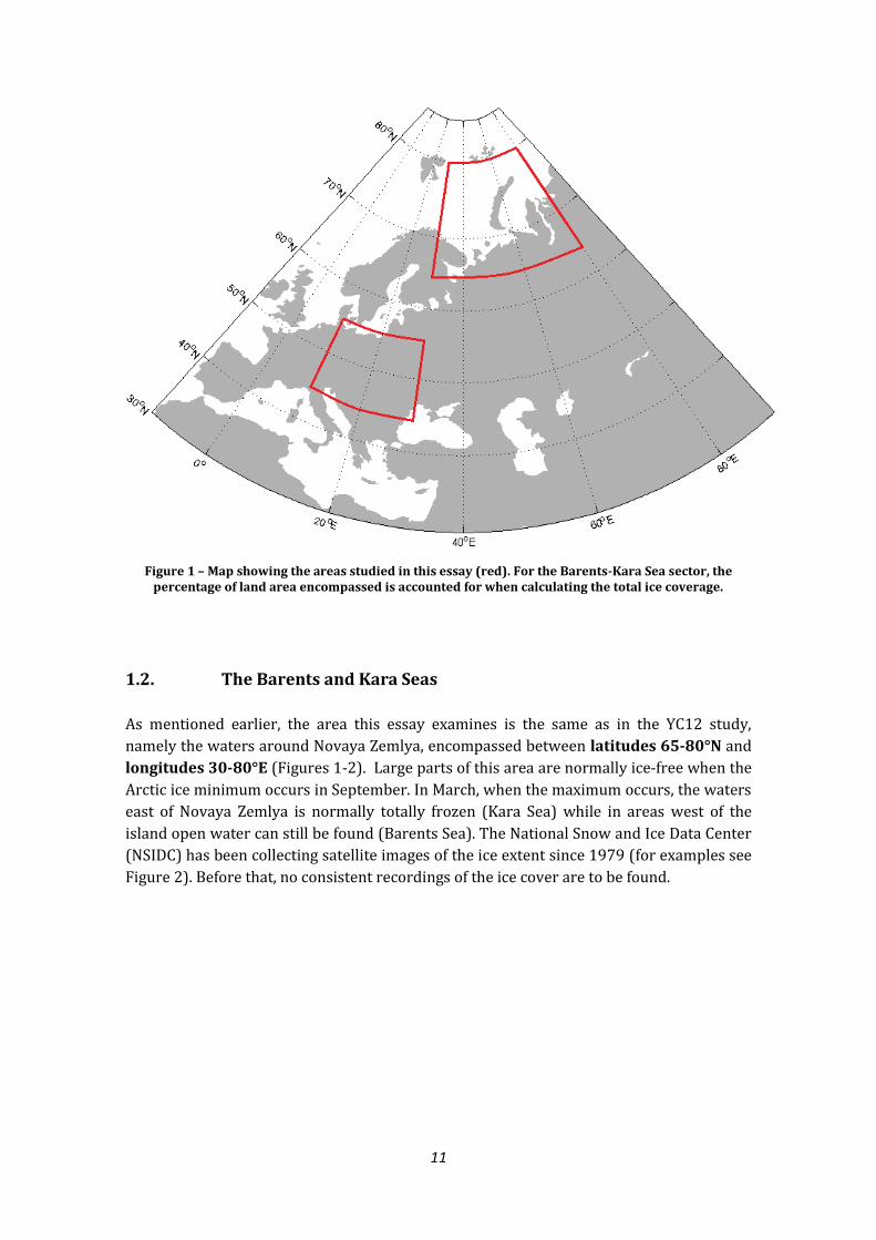
Figure 1 – Map showing the areas studied in this essay (red). For the Barents-Kara Sea sector, the percentage of land area encompassed is accounted for when calculating the total ice coverage.
1.2. The Barents and Kara Seas
As mentioned earlier, the area this essay examines is the same as in the YC12 study,
namely the waters around Novaya Zemlya, encompassed between latitudes 65-80°N and
longitudes 30-80°E (Figures 1-2). Large parts of this area are normally ice-free when the
Arctic ice minimum occurs in September. In March, when the maximum occurs, the waters
east of Novaya Zemlya is normally totally frozen (Kara Sea) while in areas west of the
island open water can still be found (Barents Sea). The National Snow and Ice Data Center
(NSIDC) has been collecting satellite images of the ice extent since 1979 (for examples see
Figure 2). Before that, no consistent recordings of the ice cover are to be found.

12
Figure 2 - Reconstruction of Arctic ice cover from satellite images by NSIDC. The figure shows the ice cover during the exceptionally low 2012-2013 ice season, for a) September b) December c) March and d) June. The ice extension border (median) for each month is marked in pink, and the area studied in this essay is marked in red. One can note that the study area both features large variations during the year, and variations between years (seen by the position of the pink line relative to the actual ice cover this very low year). One should also note that the Ob/Yenisey estuaries should not be ice covered during Arctic summer (September). This is a known graphical error in the NSIDC database. (Source: NSIDC)

13
Proxy-based reconstructions have been made on the ice cover, one of them covering the
Arctic during the full Holocene period [de Vernal et al. 2013]. This study indicates that the
waters north of Russia, and its ice extent maxima, have experienced a type of east-west
oscillation on a millennial scale during mid- to late Holocene. Another proxy based study
by Halfar et al. [2013] mainly addresses the Canadian Arctic, but is still a valuable record
due to its very high resolution and its extensive coverage of more than 600 years. The
study uses crustose coralline algae, which are very sensitive to ice formation, and
concludes that sea ice during LIA covered large parts of the (Canadian) Arctic, but that the
ice also was highly variable, at least on the sub-decadal scale.
Klimenko [2010] provides an extensive account on the Russian Arctic climate back to 1435.
The paper uses model runs, proxy data and most of all, documentary records. It lines out
every known attempt to sail the waters of the Russian Arctic; from early Dutch and English
expeditions in the 16th century, including Willem Barentsz and his disastrous voyage in the
1590s; native Russian hunting routes around Novaya Zemlya; to the complete crossing of
the Northeast Passage in 1878-1879, by Swedish explorer Adolf Erik Nordenskiöld. The
study describes the ice conditions in the Russian Arctic as very harsh up until the 19th
century - very few expeditions managed to get passed Novaya Zemlya and enter the Kara
Sea, a sea which was then called “a cellar always full of ice”.
Figure 3 - Even Nordenskiöld got stuck in the ice. His ship, Vega, froze in by late September 1878, east of Cape Chelyuskin. It remained in the ice for ten months, and in spring the expedition could continue east, being the first ship to accomplish the full Northeast Passage. (Painting by Georg von Rosen, 1886. Courtesy of Nationalmuseum, Stockholm).

14
1.3. Central Europe
This sector is also defined in the YC12 study, and will be used here as well (see Figure 4).
The area stretches from Germany in the west to Ukraine in the east, from Italy in the south
to Denmark in the north, covering latitudes 45-55°N and longitudes 10-30°E. Apart
from the Carpathians and a small stretch of the Alps, the area features mostly lowlands
with a generally humid continental climate (Köppen: Dfb). The winter (DJF) monthly mean
normally averages just below 0°C for most of the sector. One can say that the area
represents “standard” European winter climate fairly well, since it could be affected both
by large, stable Siberian High-situations from the east, as well as Atlantic cyclone activities
from the west.
Figure 4 – The Central European sector (red) and its average DJF temperatures. One can see that the mean temperature is fairly evenly distributed over the area, even though the eastern parts are somewhat colder in general. (Source: University of Wisconsin, Madison).
1.4. The North Atlantic oscillation
The NAO is of great importance when it comes to winter temperatures in Europe. A
positive phase - that is a large pressure gradient between the two main pressure centers
over the North Atlantic sector, the Icelandic low and the Azorean high – normally induces
winter cyclone activities with strong westerlies and thus wet and mild conditions over
Europe north of the Alps. A negative phase – that is a small pressure gradient between
Iceland and The Azores – results in stable winter conditions with high-amplitude slow-
moving Rossby waves, and thus often clear and cold conditions. The unusually cold
15
European winter of 2009/10 has been linked to the very low NAO-index measured that
year [Seager et al. 2010]. According to some of the studies presented earlier in the
Introduction (section 1.1), it is the NAO itself that could be affected by the anomalous heat-
fluxes related to a reduced Arctic sea ice cover, and thus in turn being the reason for the
cold winters in Europe.
A related mechanism to the NAO is often referred to as the Arctic oscillation (AO). This is
not as precisely defined as the NAO, but is sometimes regarded as basically the same
mechanism as, or at least closely connected to, the NAO. Simplified, one can say that the
AO stretches all around the globe, while the NAO is a part of it, only confined to the North
Atlantic sector. Some sources simply use of the term AO/NAO when describing this
phenomenon. This essay, however, will hereafter only use the term NAO. For a full
discussion on the differences and similarities between the AO and NAO, and what term to
use in what situation, see Ambaum et al. [2001].
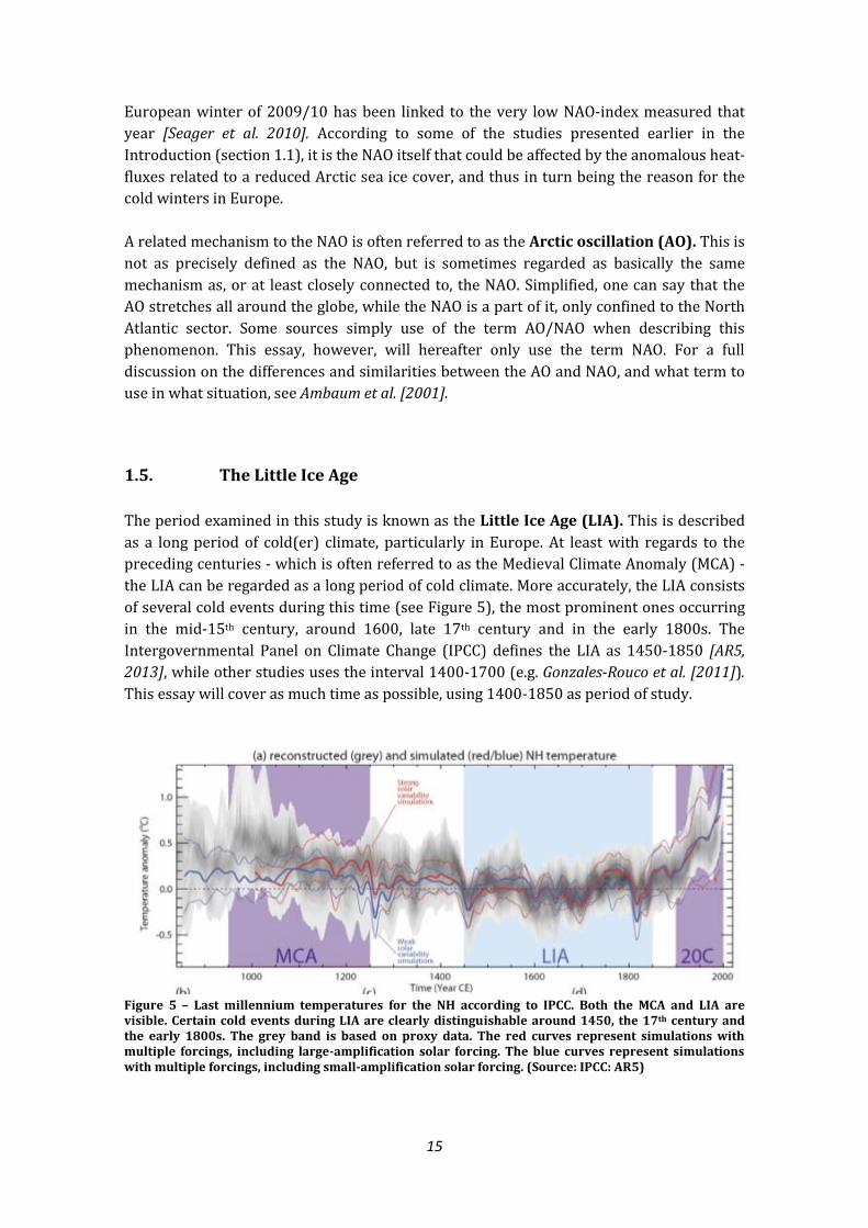
1.5. The Little Ice Age
The period examined in this study is known as the Little Ice Age (LIA). This is described
as a long period of cold(er) climate, particularly in Europe. At least with regards to the
preceding centuries - which is often referred to as the Medieval Climate Anomaly (MCA) -
the LIA can be regarded as a long period of cold climate. More accurately, the LIA consists
of several cold events during this time (see Figure 5), the most prominent ones occurring
in the mid-15th century, around 1600, late 17th century and in the early 1800s. The
Intergovernmental Panel on Climate Change (IPCC) defines the LIA as 1450-1850 [AR5,
2013], while other studies uses the interval 1400-1700 (e.g. Gonzales-Rouco et al. [2011]).
This essay will cover as much time as possible, using 1400-1850 as period of study.
Figure 5 – Last millennium temperatures for the NH according to IPCC. Both the MCA and LIA are visible. Certain cold events during LIA are clearly distinguishable around 1450, the 17th century and the early 1800s. The grey band is based on proxy data. The red curves represent simulations with multiple forcings, including large-amplification solar forcing. The blue curves represent simulations with multiple forcings, including small-amplification solar forcing. (Source: IPCC: AR5)

16
The reasons for the low temperatures during LIA are not entirely known. Explanations
including volcanic activities have been presented [Hegerl et al., 2003; Shindell et al. 2004].
That is, after a large eruption, volcanic ash is plunged into the atmosphere and will reflect
incoming sunlight during the following few years. Hence, volcanic eruptions tend to cool
the planet, at least on a shorter time scale. This essay will not assess the effect of volcanic
eruptions on the modeled historical temperature to a large extent. It will though use one
eruption (Tambora, Indonesia, 1815) as a reference for checking the model’s capability of
capturing single, historically known events, and the model’s sensitivity to volcanic forcing
(section 3.3). The Tambora eruption is known to have had severe effect on global climate;
the following year, 1816, is called ‘The Year Without a Summer’ in historical documents
[Harington, 1992; Wegmann et al, 2014].
Other explanations for the LIA concerns periods of low sunspot numbers. The most
known is the ‘Maunder minimum’, which occurred roughly 1650-1715 [Shindell et al.
2004]. A low amount of sunspot numbers simply makes the sun emit less energy, hence
cooling the Earth. The eight different variations (see section 2.2) of the model used in this
study do have different forcing configurations with regards to this, and they will be
assessed in how well they capture the Maunder minimum (section 3.3).
Discussions whether or not a consistently low NAO-index could be an explanation for the
LIA have also occurred, without proving anything. Trouet et al. [2012] has suggested the
MCA to be associated with an elevated NAO-index during medieval times. However, this
study has been discarded by Lehner et al. [2012], deeming it not robust; Trouet used proxy
records to reconstruct the historical pressure over the Atlantic, but Lehner argued that the
chosen proxy locations did not represent the full pressure pattern. Nevertheless, this
study will feature a modeled NAO-index to compare the results with. This is interesting to
include, since Seierstad & Bader [2008] (among others; see section 1.1) relate a similar
theory as in PS10 and YC12 to the NAO.
One could also discuss whether or not the LIA (and MCA) were global events or not.
Records suggest that the observed and modeled anomalies were greater in the northern
hemisphere (NH), and especially in Europe. This study does not take a stand whether the
LIA was a global event or not, but it assumes that at least part of it could be explained by
regional feedbacks, such as the mechanism suggested by PS10 and YC12.
When mentioning the term ‘capture single years’ in this essay, it should be interpreted as
the ability to model certain historical events occurring during a limited time span, e.g. a
particularly cold winter that we know from the historical records. Also, when different
members’ e treme values, e.g. their coldest and warmest years, coincide in a similar
pattern, one might also talk about the model’s capability of ‘capturing single years. This is
further assessed in the Discussion (section 4).

17
1.6. Short summary of the objectives for this study
Test if there is a historical response in CEwt to reduced BKsic during the LIA, with
data from the NASA-GISS GCM.
If yes, discuss to what extent this response might have contributed to the overall
cold conditions experienced during the LIA
If no, discuss whether such a correlation could exist, and how suitable the GISS
model is for capturing it
Include the NAO in the comparison. If a correlation is found, is the NAO correlated
in some way? If not, is the NAO still associated with colder CEwt during LIA?
2. Data and method
2.1. Data
Temperature and sea ice cover data will be extracted from the NASA-GISS-E2-R model
(National Aeronautics and Space Administration - Goddard Institute for Space Studies -
[Model]E(2) - [coupled to the] Russel [ocean model]; see Table 1). The pressure data
required for the NAO-index will be taken from the same model. All the data is originally
monthly mean, and will be presented in different seasonal variations (see sections 2.3 and
3). The handling of the data as well as producing the graphs is done in MATLAB.
2.2. Model description
As mentioned above, the model used for this study is the NASA-GISS-E2-R (hereafter only
GISS), which is used for the CMIP5/PMIP3 simulations of the last millennium. It is a global
circulation model (GCM) run for the years AD 850-1850, in an ensemble with different
forcing set-ups for volcanic aerosols, solar irradiance and land use/land cover (see later
this section). The temporal resolution, as mentioned, is on a monthly mean scale for all
stored variables. The spatial resolution is 90×144 for the whole Earth, for latitude and
longitude respectively, yielding one gridpoint every second latitude and about one
gridpoint every second-to-third longitude. Since the grid is gaussian and not geodesic, the
longitudinal resolution is higher closer to the poles, something this study benefits from.
The areas specified in Figure 1 and sections 1.2 and 1.3 then include 54 gridpoints (Central
Europe sector) and 168 gridpoints (BK sector) respectively.

18
Table 1a – Difference and similiarities between all models in the CMIP5/PMIP3 programme, with the NASA-GISS-E2-R and its eight members highlighted in red. Note that GISS is the 'largest' model in the family. The red area with the GISS model is enlarged on the next page. Note the footnote (4) attached to the members with the GRA forcing (GISS2, GISS5, GISS8). (Source: PMIP3 homepage, pmip3.lsce.ipsl.fr/).

19
Schmidt et al. [2006] describe the physics of the model thoroughly, and some
characteristics can be mentioned here. The number of vertical layers makes the model
reach above the stratosphere, turbulence is calculated at all heights and the biophysical
scheme for vegetation is advanced, including humidity. Also, freshwater fluxes from sea to
atmosphere are assumed to be at 0°C (latent heat of water vapor not dependent on
temperature). As with water vapor, it does not add to the atmospheric mass, it is not advected as
condensate and its potential energy is neglected.
As one can see in Table 1 the model ensemble consists of eight different versions of
forcing setups (hereafter called: members). Some forcings are defined by the same regime
for all these members. The vernal equinox is obviously held constant (at March 21), and
the orbital parameters are at values according to Berger [1978]. The greenhouse gases
(GHG) are also at the same, pre-industrial levels in all simulations, as defined in Joos et al.
Table 1b – Enlargement of the description of NASA-GISS-E2-R and its eight members from previous page, split in two. Note again the footnote (4) attached to the members with the GRA forcing (GISS2, GISS5, GISS8). (Source: PMIP3 homepage, pmip3.lsce.ipsl.fr/).

20
[2004]. Earth’s topography, total area covered by glaciers, the ozone level and the
tropospheric aerosols are also held constant, at pre-industrial levels.
Three of the variables do however change between the members, the first one being the
amount of volcanic aerosols. This variable comes in three different configurations: CEA,
which represents values according to Crowley et al. [2008], GRA, which is values according
to Gao [2008], and finally a configuration with no input from volcanic eruptions. The CEA
and GRA studies differs from each other in how they calculate the optical depth for the
sulphate aerosols, and how they decide what eruptions that contributed to a global
cooling; i.e. if the aerosols reached the stratosphere or not. One might note that there is a
footnote attached to the GRA configuration, saying that the applied forcing is twice as large
as it should be. This error was detected after the data was released, and thus, the members
including the GRA values are likely to overestimate the importance of volcanic eruptions.
This will be discussed more later on, and summarized for each member in Table 8 (section
3.3).
The second variable to differ between the members is the solar irradiance. This has two
different values: SBF, which represents values presented in Steinhilber et al. [2009], and
VSK + WLS back, which represents values from both Viera et al. [2011] and Wang et al.
[2005]. The two set-ups differ mainly in how much importance they give to sunspots, and
their cooling effect, especially during the Maunder minimum. The second setup (VSK +
WLS back) gives the amount of sunspots slightly ‘more weight’ than the first setup (SBF),
hence cooling the Earth more when calculating the total solar irradiance. This is also
further analyzed in Table 7 (section 3.3).
The last variable to change within the model runs is the land usage. This means how land
is assumed to have been used by humans, e.g. for agriculture or if it is deforested or not.
This variable also comes in two versions: PEA, which is defined in Pongratz et al. [2008],
and KK10, which is outlined in Kaplan et al. [2011]. The KK10 regime uses historical
population data as basis for their simulations, while PEA also includes documentary
sources, such as a large inventory of historical maps, in their reconstruction. As one might
note, the KK10 setup is only used for two of the eight GISS members.
A discussion of the forcings of the GISS model can be found in Schmidt et al. [2011].
2.3. Method
There are numerous ways to compare the selected variables in the specified areas. One
can define the winter period in different ways; one can look at the ice coverage at different
times of year; make a direct comparison or account for some time lag; one can define the
NAO somewhat differently, and one can alternate between the eight members of the model
ensemble, possibly excluding some of them.
The graphs presented in the next section could thus easily become too many. Therefore
some limitations have to be applied already here. To start with, and as mentioned earlier,

21
the geographical areas will be held constant, as defined in the YC12 study. This makes it
easy to compare the results with that study. On the other hand, this study cannot select
cold winters and years with little BKSIC in exactly the same way as in YC12, simply because
we use different models. However, if there is a correlation, one should be able to spot it
even if the criteria between the studies differ somewhat.
For the CEwt, ‘winter’ will be set to DJF in most comparisons. In some of them, however,
single months will be studied separately, in order to assess the possible temporal
variations during a single year as found in Seierstad & Bader [2008] (section 3.1.3).
The BKSIC is the variable that will be studied in most different temporal variations. If only
assessing the BKSIC mean for DJF, the variations are found to be very small, and one can
discuss whether the uncertainty of the model outweighs the small year-to-year variations
found. It also does not cover a potential feedback time-lag stemming from a low autumn
minimum in the BK region. Still, DJF BKSIC will be included since that is what is mainly
examined in YC12. Also, ONDJFM and JASONDJFM BKSIC will be compared with DJF CEWT, to
cover different possible time-lags in this hypothetic relation.
The NAO can be calculated in different ways. One can make a full pressure analysis of the
North Atlantic area with a principal component analysis (EOF-analysis, as done in e.g.
Hurrell et al [2003]), one can detect exactly where the Icelandic Low and Azorean High
have had their maxima/minima during the selected period (on average), or one can use
the ‘standard definition’, simply using the difference between the normalized sea level
pressure at two fixed locations. This study will feature the latter, using the yearly DJF
mean sea level pressure from Stykkishólmur, Iceland (65°05’N, 22°44’W) and Ponta
Delgada, Azores (37°49’N, 25°45’W), or rather, from the closest model coordinates to
these positions.
The results will be presented in three different ways: as absolute values, to be able to
match single cold years to years with little ice; as multidecadal climatological mean, to be
able to detect more long-term variations easier; and as 11-yr running mean, to correct for
possible simulated climate variations caused by the 11-yr oscillation in the solar forcing.
Scatter plots and Tables will be presented as a supplement to the graphs.
It is also of value to present not only the mean of the eight members of the GISS ensemble,
but also presenting each and every of the members. This will cover most BKSIC temporal
variations. Also, the control simulation will be presented in the results. That is, a
simulation with constant external forcing. This could be regarded as a ninth member of the
model, and will be included when calculating the mean of all members.
With regards to the data handling, to compensate for the gaussian structure of the
gridpoints in the model one cannot give every gridpoint equal weight when calculating the
mean of an area (in this case, mostly relevant for the BK area). One first has to calculate
the mean of each latitude, and from these numbers calculate the whole area mean. This is
because northern parts of the selected areas feature more gridpoints, and a direct mean
calculation would thus be misrepresenting. However, the study still benefits from the

22
gaussian grid structure, since the northern latitudinal means will be more accurate. Both
the compensation and the increased accuracy are, naturally, most relevant for the BK area.
When presenting the data in the graphs (section 3.1-3.3) a number of variables are used,
all of which are compiled in the Tables after each section. Some of the variables are also
presented under each graph in the following sections. These variables are first briefly
described below.
Every year with a DJF temperature below the mean (below the absolute mean
for the whole series) is extracted, and compared with all the years having ice
coverage below its absolute mean. The years that match (if one year features both
CEWT < mean and BKSIC < mean) are accounted for as percentage of total number of
years below the mean (WT< match. Similarly, this is also done with every year
with a DJF ice cover below its mean as a basis. This follows the same procedure
as above, and is denoted (SIC< match.
The 50 coldest years (C50) are extracted (which corresponds to ~11% of the total
years). The number of cold years who coincides with a year found among the 50
years with smallest ice cover (SIC50) is accounted for (C50-SIC50)match.
The 10 coldest years (C10) are extracted (~2% of the total years), and
comparisons with similarly low ice cover (SIC10) are made, following the same
procedure as above, yielding the variable (C10-SIC10)match.
Pearson’s correlation coefficient (R) is presented for each graph. This is a
dimensionless value between -1 and 1, and it tells us how well correlated two
curves are. If the R > 0 and close to 1, a strong positive correlation exists. If R < 0
and close to -1 a strong negative correlation exists. If R = 0, or is close to 0, the
correlation is non-existent, or negligible. Sometimes R2 is used, ‘e plained
variance’, as a more intuitive approach to describe the correlation (not in this
essay). E.g. if R = 0.5 -> R2 = 0.25 -> 25 % of the observed variance is explained by
the correlation between the two variables.
The significance of correlation (p) is presented for every graph. This is derived
from Student’s t-value (also presented) through a two-tailed significance test. If
p < 0.05, the correlation can be said to be statistically significant.
The standard deviation (σ) is presented for both ice and temperature,
respectively.

23
3. Results
This section will first feature a number of graphs, comparing BKSIC and CEWT. Each graph
will have its own figure text explaining the relevant statistical variables that cannot be
read from the graph itself. The first graph section (3.1) will be divided into three sub-
sections; one with the full ensemble of both ice and temperature data respectively, one
with seasonal ensemble mean ice-temperature comparisons, and one with ensemble mean
comparisons for individual months. In section 3.3 all eight (nine) members are plotted
individually. The graphs comparing the results with the NAO are to be found in section 3.2
and 3.3.
From section 3.1.2, the results are statistically summarized, and compiled in Tables after
each section.
For the BKsic, the ONDJFM seasonal time-span will be used mostly. This is to make sure
any eventual time-lagged effects from late summer/autumn ice is included. For the CEwt,
generally the DJF period is used (except in section 3.1.3).
3.1. Comparing BKSIC and CEWT
3.1.1. Full ensemble, ice/temperature respectively
This section will present the full ensemble of temperature and ice cover 1400-1850. This
is mainly to give the reader an overview of the data. Variations of the ice cover and the
temperature, as well as the variations between the members are seen in the graphs.
Presenting the data as both an 11-yr running mean and as a 30-yrs climatological mean is
valuable; they both give different types of overviews.
Figure 6 shows the temperature for the DJF period only. As one can see the temperature
varies quite significantly between the members. In a) the mean value manages to capture
four known cold periods during LIA, and one could spot them visually; first a cooling
around 1450, then a longer period around 1600, then the late 1600s, and finally during the
first half of the 19th century. In b) the same y-axis as in a) is kept, so that one can spot the
lesser variation in the 11-yr case. The cold periods seen in a) are barely visible here, even
if one might hint them if one knows where to look. The big ‘dip’ after 1800 by the green
member (GISS2) will be discussed later. In c), the same y-axis as a) and b) is not kept. The
refinement of the axis helps the reader to spot the slight overall cooling over the whole
period. This pre-industrial slope bears some resemblance to the famous ‘hockey stick’
based on temperature proxy data [Mann et al. 1999], though without the ‘blade’ in the 20th
century.

24
Figure 6 – DJF temperature for Central Europe, full ensemble, ensemble average value in dark blue/blue/light blue expressed as a) absolute values, b) 11-yr running mean and c) 30-yr multidecadal mean.
a)
b)
c)

25
Figure 7 shows the ice cover for the DJF period only. As one can see the ice cover varies
quite significantly between the members. In a) the variations are large, with some
relatively deep ‘dips’. However, the main interval is small in absolute numbers (oscillating
around 95%); thus, most of the sector is normally ice covered during DJF. In b) the same y-
axis are kept as in a), so that one can compare the variation of the members with the
previous graph (absolute mean vs 11-yr running). The very small scale of the variation in
DJF ice cover over the whole period is even more notable here. In c) one can really see how
small the DJF BKSIC variations are, and also note a slight slope upwards. This would,
without any statistics at hands, suggest a small negative correlation between ice and
temperature.
Figure 7 - DJF ice cover for Barents-Kara Sea, full ensemble, ensemble average value in dark green/light green/yeallow expressed as a) absolute values, b) 11-yr running mean and c) 30-yr multidecadal mean.
a)
b)
c)

26
Figure 8 is showing three variations of seasonal setup when plotting the BKsic. These
comparisons are presented to highlight the robust ice pack during winter, and the more
variable summer ice. This is to point out the importance of also including autumn ice in
the comparison later on. In a), the DJF case, one should note that this is the ‘same graph’ as
Figure 7a, but with different axes. One can easily conclude that the ice cover does not vary
very much during DJF. In b), the ONDJFM case, one can see here how much larger the
variations are when including also the late summer/autumn ice. The average value ranges
between 85-90% in this case. In c), the JASONDJFM case, one can really see the variations
of the ice, when the full summer ice from the preceding summer also is included. Scales of
all three graphs are the same.
Figure 8 – a) DJF, b) ONDJFM and c) JASONDJFM ice cover for Barents-Kara Sea, full ensemble, ensemble average value in dark green.
a)
b)
c)

27
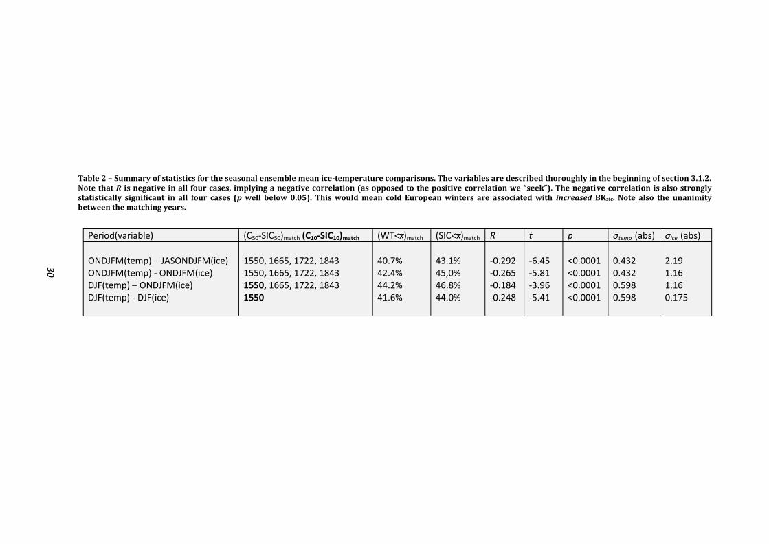
3.1.2. Ensemble means, ice-temperature comparisons, seasonal
In Figures 9-13 different seasonal comparisons between the full ensemble mean are
presented. Generally longer seasons are used for the BKSIC than for the CEWT in order to
account for a possible seasonal time-lag (i.e. Arctic late summer ice possibly affecting tem-
peratures later in autumn/winter). Red circles and squares are used to mark where SIC10
and SIC50 years match. One can almost visually see that the correlation in these graphs is
negative, not positive as we are looking for. Note in Fig. 16 that there is no match around
1640; the two dips look as they coincide, but there is a one-year difference between them.
Figure 10 - DJF temperature (blue, bottom curve) for Central Europe compared with ONDJFM BKSIC. Full ensemble mean. Light red circles show where a C10 year coincides with a SIC10 year (1550). Dark red circles show where a C50 year coincides with a SIC50 year (1550, 1665, 1722, 1843). R = -0.184, p < 0.0001.
Figure 9 – ONDJFM temperature (blue, bottom curve) for Central Europe compared with JASONDJFM BKSIC. Full ensemble mean. Dark red circles show where a C50 year coincides with a SIC50 year (1550, 1665, 1722, 1843). None of the C10 years coincides with a SIC10 year. R = -0.292, p < 0.0001.

28
Figure 11 - ONDJFM temperature (blue, bottom curve) for Central Europe compared with ONDJFM BKSIC. Full ensemble mean. Dark red circles show where a C50 year coincides with a SIC50 year (1550, 1665, 1722, 1843). Light red squares show where a C10 year coincides with a SIC10 year (1550). R = -0.265, p < 0.0001.
Figure 12 - DJF temperature (blue, bottom curve) for Central Europe compared with DJF BKSIC. Full ensemble mean. Light red circles show where a C10 year coincides with a SIC10 year (1550). None of the C50 years coincides with a SIC50 year (except of course 1550). R = -0.248, p < 0.0001.
∙
∙
∙
∙

29
In Figure 13, follows scatter plots for Figures 9-12 presented above. As can be seen all
correlations are weakly negative. The number of observations (450) makes the correlation
statistically significant (p < 0.05) in all four cases (see Table 2).
Figure 13 – Scatter plots showing the same data set as Figures 9-12.
30
Table 2 – Summary of statistics for the seasonal ensemble mean ice-temperature comparisons. The variables are described thoroughly in the beginning of section 3.1.2. Note that R is negative in all four cases, implying a negative correlation (as opposed to the positive correlation we “seek” . The negative correlation is also strongly statistically significant in all four cases (p well below 0.05). This would mean cold European winters are associated with increased BKsic. Note also the unanimity between the matching years.
Period(variable) (C50-SIC50)match (C10-SIC10)match (WT<x)̅match (SIC<x)̅match R t p σtemp (abs) σice (abs)
ONDJFM(temp) – JASONDJFM(ice) ONDJFM(temp) - ONDJFM(ice) DJF(temp) – ONDJFM(ice) DJF(temp) - DJF(ice)
1550, 1665, 1722, 1843 1550, 1665, 1722, 1843 1550, 1665, 1722, 1843 1550
40.7% 42.4% 44.2% 41.6%
43.1% 45,0% 46.8% 44.0%
-0.292 -0.265 -0.184 -0.248
-6.45 -5.81 -3.96 -5.41
<0.0001 <0.0001 <0.0001 <0.0001
0.432 0.432 0.598 0.598
2.19 1.16 1.16 0.175

31
3.1.3. Ensemble means, ice-temperature comparisons, individual months
In Figures 14-20, series of comparisons between ONDJFM BKSIC and temperatures for each
individual month is presented. This is to possibly detect the more variable connection
between different months found in Seierstad & Bader [2008] (as discussed in section 1.1).
Equal visual hints of a negative correlation can be seen here as in previous graphs.
Figure 14 - October temperature (blue, bottom curve) for Central Europe compared with ONDJFM BKSIC. Full ensemble mean. Dark red circles show where a C50 year coincides with a SIC50 year (1537, 1635, 1782). None of the C10 years coincides with a SIC10 year. R = -0.207, p < 0.0001.
Figure 15 - November temperature (blue, bottom curve) for Central Europe compared with ONDJFM BKSIC. Full ensemble mean. Dark red circles show where a C50 year coincides with a SIC50 year (1620, 1638, 1665, 1743). None of the C10 years coincides with a SIC10 year. R = -0.153, p = 0.00110.

32
Figure 16 - December temperature (blue, bottom curve) for Central Europe compared with ONDJFM BKSIC. Full ensemble mean. Dark red circles show where a C50 year coincides with a SIC50 year (1484, 1520, 1550, 1781, 1843). Light red squares show where a C10 year coincides with a SIC10 year (1484, 1520, 1550). R = -0.104, p = 0.0276.
Figure 17 - January temperature (blue, bottom curve) for Central Europe compared with ONDJFM BKSIC. Full ensemble mean. Dark red circles show where a C50 year coincides with a SIC50 year (1665, 1722). None of the C10 years coincides with a SIC10 year. R = -0.175 p = 0.000210.
∙ ∙
∙
∙ ∙ ∙

33
Figure 18 - February temperature (blue, bottom curve) for Central Europe compared with ONDJFM BKSIC. Full ensemble mean. Dark red circles show where a C50 year coincides with a SIC50 year (1502, 1505, 1522, 1550, 1665, 1722). Light red squares show where a C10 year coincides with a SIC10 year (1522). R = -0.186, p < 0.0001.
Figure 19 - March temperature (blue, bottom curve) for Central Europe compared with ONDJFM BKSIC. Full ensemble mean. Dark red circles show where a C50 year coincides with a SIC50 year (1549, 1659, 1782, 1799, 1804). None of the C10 years coincides with a SIC10 year. R = -0.153, p = 0.00110.
∙
∙

34
Figure 20 shows scatter pots for Figures 14-19 presented above. It is hard to outline any
conformity from these diagrams visually, but Table 3 tells us that the negative correlation
is statistically significant in all cases, and that December stands out somewhat from the
other months (see Table 3).
Figure 20 - Scatter plots showing the same data set as Figures 14-19.

35
Table 3 - Summary of statistics for the individual months ensemble mean ice-temperature comparisons. The variables are described thoroughly in the beginning of section 3.1.2. Note that R is negative in all six cases, implying a negative correlation also here. The negative correlation is also here statistically significant in all four cases (p well below 0.05). Note also the spread in matching years as opposed to Table 2. Note also that the December comparison stands out slightly; it has three years of (C10-SIC10)match (1484, 1520 and 1550), the highest percentages of years below mean that matches (48.6% and 50.2% respectively), and a p-value which implies some irregularities or disturbances compared to the other cases. This is further discussed in section 4.4.
Period(variable) (C50-SIC50)match (C10-SIC10)match (WT<x)̅match (SIC<x)̅match R t p σtemp (abs) σice (abs)
October(temp) - ONDJFM(ice) November(temp) - ONDJFM(ice) December(temp) - ONDJFM(ice) January(temp) - ONDJFM(ice) February(temp) - ONDJFM(ice) March(temp) - ONDJFM(ice)
1537, 1635, 1782 1620, 1638, 1665, 1743 1484, 1520, 1550, 1781, 1843 1665, 1722 1502, 1505, 1522, 1550, 1665, 1722 1549, 1659, 1782, 1799, 1804
46.3% 46.3% 48.9% 43.7% 43.3% 41.6%
48.8% 48.6% 50.2% 44.9% 44.4% 42.7%
-0.207 -0.153 -0.104 -0.175 -0.186 -0.153
-4.47 -3.27 -2.21 -3.76 -4.00 -3.27
<0.0001 0.00110 0.0276 0.000210 <0.0001 0.00110
0.568 0.639 0.795 0.855 0.835 0.657
1.16 1.16 1.16 1.16 1.16 1.16

36
3.2. Comparing NAO and CEWT
In Figure 21, the result of the reconstructed NAO-index versus the DJF CEWT is shown. As
described earlier, the NAO is created with GISS data including the difference between the
normalized sea level pressure between (the closest gridpoints to) Stykkishólmur, Iceland
and Ponta Delgada, Azores. The NAO value is dimensionless and represented by the
number on the y-axis (the NAO-number is e.g. defined in Hurrell et al [2003]. First, the
mean NAO value from all members is presented, thereafter in the next section (3.3) each
member individually.
Note that the reconstructed NAO-index and the DJF CEwt below do not seem too correlate
positively to the naked eye. It is interesting though, when looking at the statistics, that the
R-value is positive when comparing the 11yr running mean and negative when comparing
individual years. Even though the numbers are small, it could indicate a small positive
correlation between the absolute years. The difference in sign is supported by Thompson
et al [2003], which argues that the NAO is unaffected by ocean-atmosphere coupling on a
monthly and yearly scale, but well on a decadal scale.
Figure 21 - Mean NAO-index (bars) for DJF at Azores/Stykkishólmur, and 11-yr running mean DJF temperature for the Central European sector (black curve). Both variables here use the full GISS-ensemble. Note that the scales for the y-axes are offset with respect to each other. Rabs = -0.0293, R11yr = 0.0800, pabs = 0.536, p11yr = 0.0904.

37
3.3. Individual members, ice-temperature and NAO comparisons
Figures 22-37 compares the ONDJFM BKSIC – DJF CEWT relation, and its recreated NAO-
index for individual members. As seen in section 3.1.1, the members vary substantially
between each other. The members of the ensemble will be named GISS1-GISS8(9) according
to the chart presented earlier (Table 1). The comparisons described in the beginning of
section 3.1.2, (C50-SIC50)match, (C10-SIC10)match, (WT< )match and (SIC< )match are also
performed here. To assess each member individually is useful to assess the model’s
suitability for this kind of study, for example one can outline how sensitive different
members are to their respective forcing setup.
First of all, one can conclude that there is larger difference between different members
with the same seasonal setup (this section), than between different months with the
same model setup (sections 3.1.2 and 3.1.3). Especially when using longer time periods
(section 3.1.2), where the results are very similar between the runs. For example, the four
years with (C50-SIC50)match in the full ensemble variations (Figures 9-12), are the same
years in three of the configurations (years 1550, 1665, 1722, 1843). For the individual
members, the matching years themselves correlate very poorly between the members; not
a single matching year is the same in the different member runs.
GISS1 (presented in Figures 22 and 23) is forced with the CEA, SBF and PEA setups (see
section 2.2). That is, a moderate input of volcanic aerosols (as described earlier, GRA
overestimates this factor), a lesser importance of sunspots, and the standard land use
setup. As can be seen in Figure 22, the temperature-ice comparison does neither feature a
positive correlation, nor a negative. That is, during cold years in Europe, the BKSIC is not
particularly reduced, nor particularly extensive. Even though the match between low ice
years and cold winter are weak in general, the member captures the most frequently
occurring year, 1550, as a C50 year coinciding with a SIC50 year. GISS1 manages, as the only
member, to capture the consistent low NAO-index during, and after the Maunder
minimum (Figure 23), as described by Shindell et al. [2001]. The DJF temperature does not
follow this trend though. In fact, the temperature is consistently rather high for this
member. When expressed as 11-yr running mean, the temperature rarely dips down
below 0°C.
Figure 22 - GISS1, DJF temperature (blue, bottom curve) for Central Europe and ONDJFM BKSIC. None of the C10 years coincides with a SIC10 year. Dark red circles show where a C50 year coincides with a SIC50 year (1550, 1555, 1784). R = -0.0822, p = 0.0819.

38
GISS2 (Figures 24 and 25) is forced with the same parameters as GISS1, except that it has
the somewhat erroneous, doubled GRA volcanic forcing. This suggests one should be able
to more easily note the response to major volcanic eruptions in the model results. And this
is actually true in this case: several cold years are modeled in the early 1800s, the coldest
having a DJF mean of chilling -9.0°C. That is 1816, the year after the very heavy Tambora
eruption (see section 1.5). This does not mean it actually was almost 10 degrees below
zero as a mean during the winter of 1816, it rather suggests that the overestimation of
volcanic forcing in GRA in fact could be seen in some of the members using it. Other than
that, not much is to say about GISS2. The ice-temperature is strongly negatively correlated
(R = -0.193, p < 0.0001), which actually could be seen in Figure 24 by looking at how the
curves relate to each other around 1450, 1600 and 1820. As for the NAO compared to
CEWT, no correlation can be seen.
Figure 24 - GISS2, DJF temperature (blue, bottom curve) for Central Europe and ONDJFM BKSIC. Dark red circles show where a C50 year coincides with a SIC50 year (1516, 1574, 1758). None of the C10 years coincides with a SIC10 year. R = -0.193, p < 0.0001.
The Tambora eruption, followed by the ”Year Without Summer” (1816)
Figure 23 - GISS1, NAO-index (bars) and 11-yr running mean DJF temperature for Central Europe (black curve). Note that the scales for the y-axes are offset. Rabs = 0.0365, R11yr = 0.0432, pabs = 0.440, p11yr = 0.361.

39
GISS3 (Figures 26 and 27) features the same configuration as the two members above,
except that it has no volcanic forcing at all. It has seven matches of C50 and SIC50 years (the
most, together with GISS6) and an R value of almost zero, implying no correlation at all, not
positive nor negative. As for the NAO/temperature comparison, no statistically significant
correlation can be seen with this member either.
Figure 26 - GISS3, DJF temperature (blue, bottom curve) for Central Europe and ONDJFM BKSIC. Dark red circles show where a C50 year coincides with a SIC50 year (1404, 1435, 1503, 1619, 1665, 1677, 1846). None of the C10 years coincides with a SIC10 year. R = -0.00341, p = 0.943.
Figure 25 – GISS2, NAO-index (bars) and 11-yr running mean DJF temperature for Central Europe (black curve). Note that the scales for the y-axes are offset. Rabs = 0.00370, R11yr = -0.0166, pabs = 0.938, p11yr =0.726.
Figure 27 - GISS3, NAO-index (bars) and 11-yr running mean DJF temperature for Central Europe (black curve). Note that the scales for the y-axes are offset. Rabs = -0.0512, R11yr = 0.0633, pabs = 0.279, p11yr = 0.181.
40
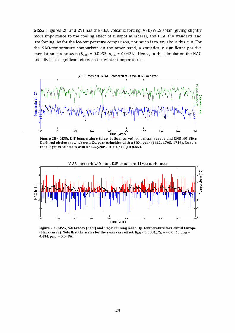
GISS4 (Figures 28 and 29) has the CEA volcanic forcing, VSK/WLS solar (giving slightly
more importance to the cooling effect of sunspot numbers), and PEA, the standard land
use forcing. As for the ice-temperature comparison, not much is to say about this run. For
the NAO-temperature comparison on the other hand, a statistically significant positive
correlation can be seen (R11yr = 0.0953, p11yr = 0.0436). Hence, in this simulation the NAO
actually has a significant effect on the winter temperatures.
Figure 28 - GISS4, DJF temperature (blue, bottom curve) for Central Europe and ONDJFM BKSIC. Dark red circles show where a C50 year coincides with a SIC50 year (1613, 1705, 1716). None of the C10 years coincides with a SIC10 year. R = -0.0212, p = 0.654.
Figure 29 - GISS4, NAO-index (bars) and 11-yr running mean DJF temperature for Central Europe (black curve). Note that the scales for the y-axes are offset. Rabs = 0.0331, R11yr = 0.0953, pabs = 0.484, p11yr = 0.0436.

41
GISS5 (Figures 30 and 31) is another GRA member, which also features KK10, the less
comprehensive of the two land use forcings (mainly using historical population as base for
configuration). Also here one can, possibly, spot the effects of the Tambora eruption: 1816
is cold here as well. Not as cold as in GISS2, but still low, at -5.5°C as DJF mean. Note also
that this is the only member that clearly indicates “The Great Frost of 1709” (discussed
further in section 4). However, both for the ONDJFM ice data and DJF temperature data,
and except for the control simulation, this member is the one who differs mostly from the
mean in absolute numbers (average 0.59 percentage units and 0.39°C below the mean). As
for the NAO though, it does see the strongest positive correlation for the 11-yr running
mean (R11yr = 0.116, p11yr = 0.0139). Looking at the graph, one might actually see some
visual correlation between the temperature and NAO-index. Note also the exceptionally
low NAO-value at 1601 (< -5), the lowest single value of one year among all member. As
already seen in this essay, the GISS members’ data vary significantly for specific individual
years.
Figure 30 - GISS5, DJF temperature (blue, bottom curve) for Central Europe and ONDJFM BKSIC. Dark red circles show where a C50 year coincides with a SIC50 year (1639, 1762). None of the C10 years coincides with a SIC10 year. R = -0.114, p = 0.0157.
”The Great Frost of 1709”
Figure 31 - GISS5, NAO-index (bars) and 11-yr running mean DJF temperature for Central Europe (black curve). Note that the scales for the y-axes are offset. Rabs = -0.000979, R11yr = 0.116, pabs = 0.984, p11yr = 0.0139.

42
GISS6 (Figures 32 and 33) is the member that matches the YC12 and PS10 theory best (or
rather, ‘least bad’). Like GISS3, it has no volcanic forcing, and matches in 7 out of the 50
coldest years. Even if not statistically significant (p = 0.515), the R value is positive as only
member (0.0308). The percentage of match in temperature/ice below mean is the highest
for the individual members (38% and 47% respectively). Also the absolute deviation from
the mean value is the smallest for this member (only 0.03°C below the mean in average).
Even if the results of this member do not, by any means, prove anything of statistically
significant value, it is interesting to note that ensemble members without volcanic forcing
match the proposed BKSIC - CEWT feedback theory best. Or again rather, least bad.
Figure 32 - GISS6, DJF temperature (blue, bottom curve) for Central Europe and ONDJFM BKSIC. Dark red circles show where a C50 year coincides with a SIC50 year (1458, 1504, 1521, 1593, 1722, 1773, 1812). None of the C10 years coincides with a SIC10 year. R = 0.0308, p = 0.515.
Figure 33 - GISS6, NAO-index (bars) and 11-yr running mean DJF temperature for Central Europe (black curve). Note that the scales for the y-axes are offset. Rabs = -0.0213, R11yr = 0.00780. σNAO = 1.42, σabs = 1.89, σ11yr = 0.684 (absolute values).

43
GISS7 (Figures 34 and 35) features CEA, VSK/WLS and KK10. The VSK/WLS (in GISS4-
GISS8) should theoretically yield colder conditions during the Maunder minimum (1650-
1715) but this cannot be seen in this member, nor in any of the others. The DJF mean
during this period are roughly the same for all members. For GISS7 not much is to say
actually. One might note the single highest value of the NAO-index around year 1800 (> 6).
Figure 34 - GISS7, DJF temperature (blue, bottom curve) for Central Europe and ONDJFM BKSIC. Dark red circles show where a C50 year coincides with a SIC50 year (1549, 1666, 1751, 1813). None of the C10 years coincides with a SIC10 year. R = -0.0295, p = 0.533.
Figure 35 - GISS7, NAO-index (bars) and 11-yr running mean DJF temperature for Central Europe (black curve). Note that the scales for the y-axes are offset. Rabs = -0.0117, R11yr = -0.0265. σNAO = 1.49, σabs = 1.79, σ11yr = 0.542 (absolute values).

44
GISS8 (Figures 36 and 37) is another GRA member where the cold year of 1816 could be
seen. Similar to GISS5, the mean DJF temperature almost reaches -6°C. As for the C50-SIC50
matches, this member has 6 of them, 5 of which in the 16th and 17th centuries
Figure 36 - GISS8, DJF temperature (blue, bottom curve) for Central Europe and ONDJFM BKSIC. Dark red circles show where a C50 year coincides with a SIC50 year (1507, 1538, 1558, 1622, 1684, 1843). None of the C10 years coincides with a SIC10 year. R = -0.186, p < 0.0001.
Figure 37 - GISS8, NAO-index (bars) and 11-yr running mean DJF temperature for Central Europe (black curve). Note that the scales for the y-axes are offset. Rabs = 0.0440, R11yr = 0.0136. σNAO = 1.42, σabs = 1.71, σ11yr = 0.615 (absolute values).

45
“GISS9” (Figure 38; no NAO simulation) is the control simulation, with constant external
forcing. One might think that it would yield results most similar to GISS3 and GISS6 (with
no volcanic forcing), but instead we find only one C50 – SIC50 match. The R numbers of
these three ‘least forced’ members coincide rather well though. As the reader might have
noticed, this ‘member’ is still included in all full ensemble mean runs in this study.
Figure 38 - "GISS9", Control simulation, DJF temperature (blue, bottom curve) for Central Europe and ONDJFM BKSIC. Dark red circles show where a C50 year coincides with a SIC50 year (1568). R = -0.0754, p = 0.111.

46
Table 4 - Summary of statistics for the individual member runs of ice-temperature comparisons. The variables are described thoroughly in the Method section (2.3). Note that R is very small (negligible) in five cases (GISS1, GISS3, GISS4, GISS6, GISS7), implying that no correlation exists for these members, no positive nor negative. This together with the high p-values in these cases (well above 0.05) prohibits us to say anything about a correlation. The other four members (GISS2, GISS5, GISS8, GISS9) provide higher (absolute) values of R, all of which are negative. The negative correlation found in these four cases can be considered statistically significant based on their p-values (below 0.05). Note the spread of the years; not any year with (C50-SIC50)match can be found more than once. Note also that not a single (C10-SIC10)match is found. Finally, the percentages of years below mean that matches are significantly lower than in Tables 2 and 3.
Member, period(variable) (C50-SIC50)match (no (C10-SIC10)match) (WT<x)̅match (SIC<x)̅match R t p σtemp (abs) σice (abs)
GISS1, DJF(temp) – ONDJFM(ice) GISS2, DJF(temp) – ONDJFM(ice) GISS3, DJF(temp) – ONDJFM(ice) GISS4, DJF(temp) – ONDJFM(ice) GISS5, DJF(temp) – ONDJFM(ice) GISS6, DJF(temp) – ONDJFM(ice) GISS7, DJF(temp) – ONDJFM(ice) GISS8, DJF(temp) – ONDJFM(ice) “GISS9”, DJF(temp) – ONDJFM(ice)
1550, 1555, 1784 1516, 1574, 1758 1404, 1435, 1503, 1619, 1665, 1677, 1846 1613, 1705, 1716 1639, 1762 1458, 1504, 1521, 1593, 1722, 1773, 1812 1549, 1666, 1751, 1813 1507, 1538, 1558, 1622, 1684, 1843 1568
35.0%, 33.2%, 34.3%, 36.1%, 31.0%, 38.3%, 33.9%, 32.5%, 34.7%,
42.7% 40.4% 41.8% 44.0% 37.8% 46.8% 41.3% 39.6% 42.2%
-0.0822 -0.193 -0.00341 -0.0212 -0.114 0.0308 -0.0295 -0.186 -0.0754
-1.74 -4.16 -0.0700 -0.450 -2.43 0.650 -0.620 -4.00 -1.60
0.0819 <0.0001 0.943 0.654 0.0157 0.515 0.533 <0.0001 0.111
1.68 1.81 1.79 1.68 1.85 1.89 1.79 1.71 1.60
3.12 3.29 3.06 3.21 3.08 2.92 2.98 3.17 3.18

47
Table 5 – Summary of years with a (C50-SIC50)match from Tables 2, 3 and 4, and how often they occur. How many of the matches that is also a (C10-SIC10)match is presented in bold print in the parenthesises. Single (C50-SIC50)match years occurring only once are not included in this Table.
Most frequently occurring years
1550: 7 (3) times 1665: 6 (0) times 1722: 6 (0) times 1843: 5 (0) times 1549: 2 (0) times 1782: 2 (0) times 1484: 1 (1) times 1520: 1 (1) times 1522: 1 (1) times

48
Table 6 - Summary of statistics for the full ensemble, and the individual members for the temperature-NAO comparisons. The variables are described thoroughly in the method section (3.2). No statistically significant correlation is found when comparing the absolute values. However, when comparing the 11-yr running mean, a small positive correlation (that is, a low NAO-index associated with lower winter temperatures) is found in two cases; GISS4 and GISS5. The p-values indicate that this correlation is statistically significant (< 0.05 . The Full Ensemble run is “close” to having a statistically significant, weak, positive correlation (p11yr = 0.09).
Member, period(variable) Rabs R11yr tabs t11yr pabs p11yr σNAO (abs) σtemp, abs (abs) σ11yr (abs)
Full ensbl, DJF(temp) – DJF(NAO-index) GISS1, DJF(temp) – DJF(NAO-index) GISS2, DJF(temp) – DJF(NAO-index) GISS3, DJF(temp) – DJF(NAO-index) GISS4, DJF(temp) – DJF(NAO-index) GISS5, DJF(temp) – DJF(NAO-index) GISS6, DJF(temp) – DJF(NAO-index) GISS7, DJF(temp) – DJF(NAO-index) GISS8, DJF(temp) – DJF(NAO-index)
-0.0293 0.0365 0.00370 -0.0512 0.0331 -0.000979 -0.0213 -0.0117 0.0440
0.0800 0.0432 -0.0166 0.0633 0.0953 0.116 0.00780 -0.0265 0.0136
-0.620 0.770 0.0800 -1.08 0.700 -0.0200 -0.450 -0.250 0.930
1.70 0.910 -0.350 1.34 2.02 2.47 0.160 -0.560 0.290
0.536 0.440 0.938 0.279 0.484 0.984 0.653 0.805 0.352
0.0904 0.361 0.726 0.181 0.0436 0.0139 0.869 0.575 0.774
1.12 1.78 1.49 1.43 1.37 1.40 1.42 1.49 1.42
0.596 1.68 1.81 1.79 1.68 1.85 1.89 1.79 1.71
0.299 0.488 0.769 0.573 0.575 0.616 0.684 0.542 0.615

49
Table 7 – Summary of each member’s response to solar forcing during ‘the Maunder Minimum’ 1650-1715. The four members with no or little sunspot importance show slightly milder DJF conditions during this period (0.18°C warmer on average). That is, the different forcings seems to matter in this case.
Member Solar forcing DJF mean 1650-1715 (°C) Mean (°C)
GISS9 (control) None -1.09
-1.53 GISS1
SBF (sunspots less important)
-1.61
GISS2 -1.90
GISS3 -1.52
GISS4 VSK + WLS back (sunspots more important)
-1.37 -1.71
GISS5 -2.18
GISS6 -1.70
GISS7 -1.95
GISS8 -1.37
Table 8 - Summary of each member’s response to volcanic forcing the years after the Tambora eruption 1815. The three members with exaggerated volcanic forcing (GRA) show much lower temperatures (1.16°C colder on average) during these years than the members with weaker volcanic forcing (CEA). In turn, the CEA members are 0.54°C colder than the members with no volcanic forcing. That is, the different forcings definitely matters in this case.
Member Volcanic forcing DJF mean 1815-1820 (°C) Mean (°C)
GISS2 GRA (strong volcanic)
-3.58 -2.92 GISS5 -2.30
GISS8 -2.89
GISS1 CEA (weak volcanic)
-1.74 -1.76 GISS4 -2.04
GISS7 -1.49
GISS3 None
-1.71 -1.32 GISS6 -1.42
GISS9 (control) -0.83

50
4. Discussion
4.1. General overview of the results
The first thing that strikes you when studying the result section in this paper is the lack of
positive correlation between reduced BKSIC and cold European winters as described in
YC12 and PS10. Rather, a negative correlation can be seen. That would be, during cold
winters the Barents and Kara Seas are more covered by sea ice, contradictory against the
postulated PS10 and YC12 theory. This is best seen in Figures 9-13, but can be spotted
throughout the results section. It can also be seen in Tables 2-4; the Pearson’s correlation
coefficients (R) are constantly negative, implying a negative correlation. The significance
of correlation is strong (p < 0.05) in all the full ensemble runs (Figures 9-20) but mostly
weak (p > 0.05) for the individual member runs (Figures 22-38).
As summarized in Table 5, not many of the coldest years coincide with years of
reduced sea ice (C50-SIC50 and C10-SIC10). For a normal run, around 3 out of 50 (the ‘range’
is from 1 to 7 out of 50 years) and around 1 out of 10 (only once do more than 1 out of 10
years match) of the coldest European years respectively, match a year with low BKSIC. Only
one year occurs frequently in all the different types of investigations, namely 1550. That,
could be said, does not really support YC12 either. Nor does the percentage of the
matching years with temperature/ice cover below mean do either. The interval in the
comparisons lies between 30-50% (highest value: 50.2%). That, again, would also imply a
slightly negative correlation. It is hard to know what result to expect from these year-to-
year tests though. If there actually were a correlation, how many C50-SIC50 matches would
one see? Again, difficult to say, but one could at least expect more than seen in this essay.
If using the exact same seasonal setup as YC12 (the DJF-DJF comparison) the results are
notably insignificant (Figure 12). As highlighted in section 3.1.1 though, the variations of
ice cover during the winter are very small, making this type of model-based study difficult
for a DJF-DJF comparison. One can discuss whether the variations are within the error
margin of the model in this case.
Not to forget is the study by Klimenko [2010]. It gives an important hint that the real ice
conditions in the Russian Arctic during LIA in fact were rather severe. That is, another
source that speaks against the YC12 and PS10 theory, and its validity during the LIA. It is
not for nothing a sea like the Kara Sea is dubbed ‘a cellar always full of ice’. That is, Willem
Barentsz should not be too ashamed that he failed to reach further than Novaya Zemlya
back in 1596.
With that being said, this study alone cannot disprove YC12, or similar studies either.
There are many different ways to perform this kind of study, and this essay does not cover
them all. First of all, the YC12 study uses a different ensemble of models than this one.
Different models can have different configurations, some of which does not manage to
capture the exact feedback mechanism that is the background for this hypothesis.

51
4.2. How suitable is the GISS model for this kind of study?
Of course, it might be so that a cold CEWT - low BKSIC relation does exist in reality, but the
GISS model fails to capture it. This can be due to various weaknesses in the model;
inabilities to capture single events with limited time-span, different feedback effects than
those included in the model configuration etc. Boé et al. [2009] discusses the problems
GCMs have with capturing Arctic/midlatitudes feedback effects, for example describing
the Arctic atmosphere and the difficulties to model its response to the strong temperature
inversions occurring in Polar regions.
A sign that the GISS model does not capture single historical events very well can be
found in the archives. The Great Frost of 1709 is a well-known, very cold winter
throughout Europe, especially in the Central-Eastern parts which this study focuses on.
This area saw temperatures of 6-8°C below mean (1971-2000 climatology) during January
and February 1709, which were the most extreme months [Luterbacher et al. 2004]. Other
parts of Europe featured both severe famine and ice skating (frequently reproduced on
paintings from this time) on frozen rivers, during this ‘coldest winter in 500 years’ [Pain,
2009]. However, only one member of the GISS ensemble captures this cold spell (GISS5,
stating a mean DJF temperature of –7.1°C in our selected area). Luterbacher also argues
that this cold spell was accompanied by, or partly caused by, a negative value of the NAO-
index. A negative value is, however, modeled by four out of eight members (GISS1, GISS2,
GISS3, GISS8; -1.04, -3.15, -2.07, -2.60 respectively).
Be that as it may, one should be careful judging GCMs like this for failing to capture certain
historical events like this, with limited, temporal span, in limited areas. Their task is to
model climate, not weather. We do not know for sure what caused this very severe
winter; it could be due to a wide range of more or less random factors and forcings, some
of which not at all included in standard GCM configurations.
So, one should remember that a climate model more is a representation of its own
created reality, with its own atmosphere, forcings and feedbacks, more than a window
back in time. Of course, it follows the same physical laws as reality does, but it should not
be used as a historical lexicon. This obviously makes it harder to capture mechanisms back
in time that are limited to shorter time spans, like the YC12 theory. Nevertheless, nothing
says that this physically described, feedback couldn’t exist and be correctly reproduced
within the constructed atmosphere existing in this model.
In fact, the model does capture some known events over shorter time-spans (the
Maunder minimum and the Tambora eruption). These are strongly connected to the
ensemble’s different forcing configurations, which we do know are defined rigorously in
the model. This can be seen in section 3.3 and in Tables 7-8. This strengthens the
assumption of GISS as a reliable model. One might argue that these factors have nothing to
do with the YC12 theory and the purpose of this study. But let us assume the model would
have been totally unable to even capture the Tambora eruption or the Maunder minimum,
even though the model has strong volcanic and solar forcings; then one could have
discussed whether or not the GISS model should have been discarded instead of the YC12
theory.

52
4.3. Large difference between each member
The main outcome of the each-member-analysis in section 3.3 is that all the members
differ significantly between each other (seen in Table 4) and that they respond well to
their respective forcing setup. One also notes that none of the members finds the
relationship outlined in YC12, PS10 and similar studies, but that GISS6 describes it best, or
rather, least bad. With regards to the forcings, one can conclude that the members with the
GRA setup do respond very well to their volcanic aerosol forcing, since the Tambora
eruption of 1815 actually could be spotted in all three cases (Table 8). If one were to
exclude member(s) from the ensemble, perhaps the three (incorrectly calibrated) GRA
members are in the risk zone; at least one of them (GISS2) has shown tendencies to
overestimate the volcanic aerosol cooling effect, at least for this specific case. One might
also note the large statistical difference within specific members. This further manifests
the large variability they show on a single year-level, and invites to discussion whether or
not this model is suitable for this kind of study. This concerns mostly the temperature-
NAO comparisons in section 3.3, and the difference between pabs and p11yr for GISS5 and
GISS6 seen in Table 6. This particular case, however, is briefly discussed in section 3.2, and
further outlined in Thompson et al. [2003].
4.4. A hint of correlation after all?
The study does see a small correlation though, or a hint of a correlation, with respect to
the results of Seierstad & Bader [2008] discussed in section 1.1. It can be seen when
comparing the ONDJFM BKSIC with DJF CEWT of individual months (section 3.1.3). Or rather,
it does not prove any connection, since the results are pretty vague, but it sees a similar
pattern. The Seierstad & Bader study found a time-lag, implying that a low ice cover in
autumn affects mostly the late winter cyclone activity. This would resemble the negative
phase of the NAO, and yield colder temperatures in Europe. This study’s investigation of
each single month, does see December and February-March standing out. These three
months see the highest frequencies of C50-SIC50 (and C10-SIC10) matches, at least for the full
ensemble average case. The numbers are not high by any means, but stand out in
comparison to other months (October, November, January). The overall percentage of
years below mean that matches also stands out somewhat in the dataset (again, see Table
3). This might be a hint that a time-lagged atmospheric response, similar to that
investigated by Seierstad and Bader, is captured by the GISS model. However, when
looking at the R and p-values, a statistically significant negative correlation is still seen.
Not as much for the December case, but still for February and March. This maybe leaves
this hint at only a hint. But it could suggest that if the BKsic and CEwt were to be
associated, it could be variable on a month-to-month basis, as in Seierstad and Bader,
rather than uniform over longer seasons, as suggested in PS10 and YC12.

53
4.5. Central European winter temperatures and the NAO
The NAO was originally thought to be included in this study to have another parameter to
compare with in cases the YC12 correlation was found. Now, no such correlation was
confirmed, but the NAO is still valuable to apply on the data. What can be seen from the
NAO data (section 3.2 and 3.3) is interesting. The visual analysis of the NAO-curves does
not satisfy the reader at a first glance, but when studying the statistics deeper (Table 6)
one actually finds a positive correlation for GISS5 and GISS6. As mentioned in section 4.3,
this correlation is confined to the 11-yr running mean comparisons. Maybe even more
interesting is that the full ensemble mean (Figure 21) features a, small, positive
correlation with an R-value for absolute years which almost could be considered to be
statistically significant (p = 0.09). At least when comparing to the R-value for the 11-yr
running mean, which is negative, and not statistically significant (p = 0.6). This might lead
the reader into believing that fluctuations in the NAO-index actually could have played a
role for the low temperatures during LIA. However, the numbers itself are rather small.
4.6. Could the theory still be valid?
There is an obvious difference between YC12 and this study: YC12 focuses on two future
model scenarios, the moderate emissions scenario RCP4.5 and the heavy emissions
scenario RCP8.5, (as well as a short historical time span of ~50 years, for which it does not
find a correlation) with generally much less ice due to the projected global warming. It is
possible that this presumed feedback includes some kind of threshold which is passed for
future, global warming-related, lighter ice conditions, but not for historical ice scenarios. It
is clear that we today have large fluctuations in the Arctic sea ice cover, which might make
it easier for the open water to actually have an effect on the water-atmosphere heat
exchange, and subsequently on larger-scale circulation patterns. In short, today’s high
year-to-year Arctic sea ice variability might have passed this kind of threshold, yielding
this feedback (seen in the YC12 future scenarios), a threshold which was not passed
during the LIA (seen in this study).
This study was based on an assumption of a warm-Arctic cold-Europe anomaly. Or rather
reduced-sea-ice-Arctic, but that would also imply warm. However, this anomaly was not
found. If some conclusions were to be drawn already here, the study has rather showed
the opposite. Yet, the study alone cannot totally disprove the theories upon which it was
built. This is something that should be stressed; this is merely one of many possible type
of studies on the topic, with one of many possible models.

54
5. Conclusions
This study has investigated the relationship between sea ice reduction in the Arctic and
cold winters in Europe on a historical basis in a climate model simulation. The essay was
based on theories presented in two studies, here referred to as YC12 and PS10, but other
important studies were found along the way, e.g. Seierstad & Bader [2008]. In short, it can
be said that this study tried to confirm the YC12 and PS10 studies on a historical basis.
However, the results obtained from the GCM (NASA-GISS) did not support the theory. If
a correlation was found over time, it was not that years with lighter ice were associated to
cold winters, but rather the opposite.
Why this study yielded a lack of correlation has also been discussed, and one probable
explanation is that, if the mechanism were to exist, it might not be noticeable until a
threshold is passed. This threshold would then be when there is enough open sea in the
Arctic that can affect the ocean-atmosphere heat flux, and hence the larger scale
circulation patterns. It is speculated that this threshold is passed for future global
warming scenarios (e.g. YC12), but not in this historical study.
The NAO index was also examined and modeled for the historical period (1400-1850), and
a weak correlation with Central European winter temperatures could be found, at least
for some members. However, the correlation seen in general remains weak, and overall it
seems like other factors sparked (both the known and simulated) cold conditions in
Central Europe during the LIA.
It was also discussed whether or not the GISS model was suitable for this kind of study.
One might think that for a study like this, the model must be able to precisely outline ice
and temperature variations on a year-to-year basis. This is hard, since a GCM like this
models climate, not weather. The model should not be e pected to ‘capture single years’ of
known historical events. However, a test with some known events did show that the model
actually captured some of these (e.g. the Tambora eruption and the Maunder minimum).
But again, these are events with causes that are clearly included in the model forcing setup,
as opposed to the YC12 and PS10 theories, which might include some factors and
feedbacks not entirely understood. With that being said, since the theory (at least as
outlined in PS10) builds purely on physical mechanisms, and since physical laws definitely
are followed in the model, nothing says that the postulated correlation couldn’t have been
captured in a study like this.
However, a hint of a correlation could be found after all. Not statistically significant, but
maybe following the same pattern as outlined in the Seierstad & Bader study. That is,
that the autumn/winter sea ice cover might yield diverging effects for different months. In
this study December stood out the most, as compared to March in Seierstad & Bader
[2008]. The conclusions that can be drawn from this are not many, but at least it suggests
that a feedback mechanism like this, if it were to exist, could be variable on a month-to-
month basis, rather than uniform over longer seasons.

55
Nevertheless, this study certainly invites to more studies on the topic. Even if it does not
support the proposed theory, the study alone does not disprove it either. Again, there
are numerous ways of conducting this kind of study; the models to use could be of higher
resolution and the parameters to investigate could be more numerous. Given the
complexity of the Arctic; its feedback effects, many of which not fully understood; and its
sensitive climate in general, I look forward to further investigations of its captivating
nature.

56
Acknowledgements
I wish to thank a number of people for their contribution to this thesis. First of all, my
supervisor at Uppsala University, Hans Bergström. At Uppsala, valuable feedback has also
been received from Erik Sahlée, Anna Rutgersson and Conny Larsson. I also wish to thank
members of the Griffin group at Stockholm University; Anders Moberg, for sharing a lot of
his inspiration and ideas, Qiong Zhang, for sharing large amounts of climate data, and
Fredrik Charpentier Ljungqvist as well as Alistair Hind, for their valuable inputs and help.
Finally, I wish to thank Hanna, for her great amount of support and patience.

57
References
[1] Alexander, M. A. Bhatt, U. S. Walsh, J. E. Timlin, M. S. Miller, J. S. & Scott, J. D. (2004). The atmospheric response to realistic Arctic sea ice anomalies in an AGCM during winter. Journal of climate, 17(5), 890-905.
[2] Ambaum, M. H. Hoskins, B. J. & Stephenson, D. B. (2001). Arctic oscillation or North Atlantic
oscillation?. Journal of Climate, 14(16), 3495-3507.
[3] Berger, A. (1978). Long-term variations of caloric insolation resulting from the Earth's orbital elements. Quaternary Research, 9(2), 139-167.
[4] Boé, J. Hall, A. & Qu, X. (2009). Current GCMs' unrealistic negative feedback in the Arctic.
Journal of Climate, 22(17), 4682-4695.
[5] Cohen, J. L., J. C. Furtado, M. A. Barlow, V. A. Alexeev and J. E. Cherry. (2012). Arctic warming, increasing snow cover and widespread boreal winter cooling. Environmental Research Letters 7(1).
[6] Crowley, T. J. Zielinski, G. Vinther, B. Udisti, R. Kreutz, K. Cole-Dai, J. & Castellano, E. (2008).
Volcanism and the little ice age. PAGES news, 16(2), 22-23.
[7] Francis, J. A. and S. J. Vavrus (2012), Evidence linking Arctic amplification to extreme weather in mid-latitudes, Geophys. Res. Lett. 39, L06801, doi:10.1029/2012GL051000.
[8] Gao, C. Robock, A. & Ammann, C. (2008). Volcanic forcing of climate over the past 1500 years:
An improved ice core‐based inde for climate models. Journal of Geophysical Research: Atmospheres (1984–2012), 113(D23).
[9] Ghatak, D., C. Deser, A. Frei, G. Gong, A. Phillips, D. A. Robinson and J. Stroeve. (2012). Simulated Siberian snow cover response to observed Arctic sea ice loss, 1979-2008. Journal of Geophysical Research-Atmospheres 117.
[10] Gonzalez-Rouco, J. F. Fernández-Donado, L. Raible, C. C. Barriopedro, D. Lutherbacher, J.
Jungclaus, J. H. Swingedouw, D. Servonnat, J. Zorita, E. Wagner, S. & Ammann, M. (2011). Medieval Climate Anomaly to Little Ice Age transition as simulated by current climate models. PAGES news, 19(1), 7-8.
[11] Grassi, B., G. Redaelli and G. Visconti. (2013). Arctic Sea Ice Reduction and Extreme Climate Events over the Mediterranean Region. Journal of Climate 26(24):10101-10110.
[12] Halfar, J. Adey, W. H. Kronz, A. Hetzinger, S. Edinger, E. & Fitzhugh, W. W. (2013). Arctic sea-
ice decline archived by multicentury annual-resolution record from crustose coralline algal proxy. Proceedings of the National Academy of Sciences, 110(49), 19737-19741.
[13] Harington, C. R. (1992), The Year Without a Summer - World Climate in 1816, 576 pp. Can.
Mus. of Nature, Ottawa, Ont. Canada, 1992.
[14] Hegerl, G. C. T. J. Crowley, S. K. Baum, K.-Y. Kim, and W. T. Hyde. (2003). Detection of volcanic, solar and greenhouse gas signals in paleo-reconstructions of Northern Hemispheric temperature, Geophys. Res. Lett. , 30 (5), 1242, doi:10.1029/2002GL016635.
[15] Honda, M., Inoue, J., & Yamane, S. (2009). Influence of low Arctic sea‐ice minima on anomalously cold Eurasian winters. Geophysical Research Letters, 36(8).

58
[16] Hurrell, J.W., Kushnir, Y., Ottersen, G. & Visbeck, M. (2003). The North Atlantic Oscillation: Climate Significance and Environmental Impact. Eds. Geophysical Monograph Series, 134, 279pp.
[17] Inoue, J., Hori, M. E., & Takaya, K. (2012). The Role of Barents Sea Ice in the Wintertime Cyclone Track and Emergence of a Warm-Arctic Cold-Siberian Anomaly. Journal of Climate, 25(7).
[18] Intergovernmental Panel on Climate Change (IPCC; 2013), Fifth Assessment Report (AR5), Working Group I (WGI), The Physical Science Basis.
[19] Joos, F. S. Gerber, I. C. Prentice, B. L. Otto-Bliesner, and P. J. Valdes (2004), Transient
simulations of Holocene atmospheric carbon dioxide and terrestrial carbon since the Last Glacial Maximum, Global Biogeochem. Cycles, 18, GB2002, doi:10.1029/2003GB002156.
[20] Kaplan, J. O. Krumhardt, K. M. Ellis, E. C. Ruddiman, W. F. Lemmen, C. & Goldewijk, K. K.
(2011). Holocene carbon emissions as a result of anthropogenic land cover change. The Holocene, 21(5), 775-791.
[21] Klimenko, V. V. (2010). A Composite Reconstruction of the Russian Arctic Climate Back to AD
1435. In The Polish Climate in the European Context: An Historical Overview (pp. 295-326). Springer Netherlands.
[22] Lehner, F. Raible, C. C. & Stocker, T. F. (2012). Testing the robustness of a precipitation proxy-
based North Atlantic Oscillation reconstruction. Quaternary Science Reviews, 45, 85-94.
[23] Liu, J. P., J. A. Curry, H. J. Wang, M. R. Song and R. M. Horton. (2012). Impact of declining Arctic sea ice on winter snowfall. Proceedings of the National Academy of Sciences of the United States of America 109(11):4074-4079.
[24] Luterbacher, J. Dietrich, D. Xoplaki, E. Grosjean, M. & Wanner, H. (2004). European seasonal
and annual temperature variability, trends, and extremes since 1500. Science, 303(5663), 1499-1503.
[25] Mann, Michael E.; Bradley, Raymond S.; Hughes, Malcolm K. (1999), "Northern hemisphere
temperatures during the past millennium: Inferences, uncertainties, and limitations", Geophysical Research Letters 26 (6): 759, doi:10.1029/1999GL900070.
[26] Overland, J. E. & Wang, M. (2010). Large‐scale atmospheric circulation changes are associated
with the recent loss of Arctic sea ice. Tellus A, 62(1), 1-9.
[27] Pain, S. (2009). The year that Europe froze solid. New Scientist, 201(2694), 46-47.
[28] Petoukhov, V. and V. A. Semenov (2010), A link between reduced Barents‐Kara sea ice and cold winter extremes over northern continents, J. Geophys. Res. 115, D21111, doi:10.1029/2009JD013568.
[29] Pongratz, J. C. Reick, T. Raddatz, and M. Claussen (2008), A reconstruction of global
agricultural areas and land cover for the last millennium, Global Biogeochem. Cycles, 22, GB3018, doi:10.1029/2007GB003153.
[30] Schmidt, G.A., et al. 2006. Present day atmospheric simulations using GISS ModelE: Comparison to in-situ, satellite and reanalysis data. J. Climate, 19, 153-192, doi:10.1175/JCLI3612.1.
[31] Schmidt, G. A. Jungclaus, J. H. Ammann, C. M. Bard, E. Braconnot, P. C. T. J. D. G. Crowley, T. J.
G. Delaygue, F. Joos, N. A. Krivova, R. Muscheler, B. Otto-Bliesner, J. Pongratz, D. T. Shindell, S. K. Solanki,, F. Steinhilber & Vieira, L. E. A. (2011). Climate forcing reconstructions for use in PMIP simulations of the last millennium (v1. 0). Geoscientific Model Development, 4(1).

59
[32] Screen, J. A. and I. Simmonds. (2013). Exploring links between Arctic amplification and mid-latitude weather. Geophysical Research Letters 40(5):959-964
[33] Seager, R. Y. Kushnir, J. Nakamura, M. Ting, and N. Naik (2010), Northern Hemisphere winter snow anomalies: ENSO, NAO and the winter of 2009/10, Geophys. Res. Lett. 37, L14703, doi:10.1029/2010GL043830.
[34] Seierstad, I. A. & Bader, J. (2009). Impact of a projected future Arctic sea ice reduction on
extratropical storminess and the NAO. Climate dynamics, 33(7-8), 937-943.
[35] Shindell, D. T. Schmidt, G. A. Mann, M. E. Rind, D. & Waple, A. (2001). Solar forcing of regional climate change during the Maunder Minimum. Science, 294(5549), 2149-2152.
[36] Shindell, D. T. G. A. Schmidt, M. E. Mann, and G. Faluvegi (2004), Dynamic winter climate
response to large tropical volcanic eruptions since 1600, J. Geophys. Res. 109, D05104, doi:10.1029/2003JD004151.
[37] Steinhilber, F. Beer, J. & Fröhlich, C. (2009). Total solar irradiance during the Holocene.
Geophysical Research Letters, 36(19), L19704.
[38] Thompson, D. W. J., Lee, S., Baldwin, M. P. (2003). Atmospheric Processes Governing the Northern Hemisphere Annular Mode / North Atlantic Oscillation, Geoph. Monog. 134, pp.81-112.
[39] Trouet, V. Scourse, J. D. & Raible, C. C. (2012). North Atlantic storminess and Atlantic
Meridional Overturning Circulation during the last millennium: reconciling contradictory proxy records of NAO variability. Global and Planetary Change, 84, 48-55.
[40] de Vernal, A. Hillaire-Marcel, C. Rochon, A. Fréchette, B. Henry, M. Solignac, S. & Bonnet, S.
(2013). Dinocyst-based reconstructions of sea ice cover concentration during the Holocene in the Arctic Ocean, the northern North Atlantic Ocean and its adjacent seas. Quaternary Science Reviews.
[41] Vieira, L. E. A. Solanki, S. K. Krivova, N. A. & Usoskin, I. (2011). Evolution of the solar
irradiance during the Holocene. arXiv preprint arXiv:1103.4958.
[42] Wang, Y. M. Lean, J. L. & Sheeley Jr, N. R. (2005). Modeling the Sun's magnetic field and irradiance since 1713. The Astrophysical Journal, 625(1), 522.
[43] Wegmann, M., S. Broennimann, J. Bhend, J. Franke, D. Folini, M. Wild, and J. Luterbacher.
(2014). Volcanic influence on European summer precipitation through monsoons: Possible cause for "Year Without a Summer". J. Climate. doi:10.1175/JCLI-D-13-00524.1, [in press]
[44] Yang, S. & Christensen, J. H. (2012). Arctic sea ice reduction and European cold winters in
CMIP5 climate change experiments. Geophysical Research Letters, 39(20).

60

Tidigare utgivna publikationer i serien ISSN 1650-6553 Nr 1 Geomorphological mapping and hazard assessment of alpine areas in Vorarlberg, Austria, Marcus Gustavsson Nr 2 Verification of the Turbulence Index used at SMHI, Stefan Bergman Nr 3 Forecasting the next day’s maximum and minimum temperature in Vancouver, Canada by using artificial neural network models, Magnus Nilsson
Nr 4 The tectonic history of the Skyttorp-Vattholma fault zone, south-central Sweden, Anna Victoria Engström Nr 5 Investigation on Surface energy fluxes and their relationship to synoptic weather patterns on Storglaciären, northern Sweden, Yvonne Kramer Nr 274 Unravelling Temporal Geochemical Changes in the Miocene Mogan and Fataga group ignimbrite succession on Gran Canaria, Canary Islands, Spain. Peter A. Nicholls, February 2014 Nr 275 Time Lapse VSP Monitoring of Small scale Injected CO2 in the Frio Formation, Texas, USA. Ershad Gholamrezaie, February 2014 Nr 276 A 2D Electrical Resistivity Survey of Palsas in Tavvavuoma, sub-arctic Sweden. Per Marklund, Mars 2014
Nr 277 Metamorphic Evolution of the Middle Seve Nappe in the Snasahögarna area, Scandinavian Caledonides. Åke Rosén, Mars 2014
Nr 278 Analogue Modelling of Ductile Deformation at Competent Lenses in Grängesberg, Bergslagen, Sweden. Sara Eklöf, Mars 2014
Nr 279 Stable Isotope Systematics of Skarn-hosted REE-silicate - Magnetite Mineralisations in Central Bergslagen, Sweden. Fredrik Sahlström, Mars 2014
Nr 280 Analys av växthusgasflöden och omgivningens påverkan på turbulens vid Erssjön – en typisk svensk skogssjö. Nitzan Cohen, Mars 2014
Nr 281 A Study of the Short-term Variability of Seawater pCO2 near Östergarnsholm.
Jennie Persson Söderman, Mars 2014
Nr 282 Prediction of the Start of the Rainy Season in West Africa. Eric Sönnert, Mars 2014
Nr 283 NAO Index: An Extreme Pressure Approach. Patrik Boström, April 2014
Nr 284 Deformation, Metamorphism and Remobilisation in the Hornkullen Polymetallic Deposit, Western Bergslagen, Sweden. Stefan Andersson, April 2014
Nr 285 Prediction of Ice Flow on Storglaciären from Mass Balance Measurements Using ArcGIS. KevinMcClain, April 2014

Top Related