


Languages
Pages
Legal


DISS. ETH NO. 22898
On the model reduction for chemicaland physical kinetics
A thesis submitted to attain the degree of
DOCTOR OF SCIENCES of ETH ZURICH
(Dr. sc. ETH Zurich)
presented by
Mahdi KooshkbaghiMSc in Mechanical Engineering,
Amirkabir University of Technology(Tehran Polytechnic)
born on 25.01.1986citizen of Iran
accepted on the recommendation of
Prof. Dr. Konstantinos Boulouchos, examinerDr. Christos E. Frouzakis, co-examinerProf. Dr. Ilya V. Karlin, co-examiner
Prof. Dr. Ioannis G. Kevrekidis, co-examiner
2015


Abstract
The need to design of efficient combustion systems with minimal emissions
of pollutants has led to the development of large detailed reaction mech-
anisms for combustion involving hundreds of chemical species reacting in
a complex network of thousands of elementary reactions. Incorporating
such a detailed reaction mechanism into multidimensional simulations is
practically impossible. Different methodologies have been proposed for the
reduction of detailed mechanisms. In the present work, model reduction
approaches based on timescale separation and thermodynamic analysis are
revisited, introduced, validated and used.
First, an algorithm based on the Relaxation Redistribution Method
(RRM) is revisited and modified for constructing the Slow Invariant Mani-
fold (SIM) of a chosen dimension to cover a large fraction of the admissible
composition space that includes the equilibrium and initial states. The
manifold boundaries are determined with the help of the Rate Controlled
Constrained Equilibrium method, which also provides the initial guess for
the SIM. The latter is iteratively refined until convergence and the con-
verged manifold is tabulated. The global realization of the RRM algorithm
is applied to hydrogen-air mixtures.
Second, Spectral Quasi-Equilibrium Manifold (SQEM), which is based
on the entropy maximization under constraints built by the slowest eigen-
vectors at equilibrium, is proposed to construct the slow manifold for com-
i

Abstract
bustion mechanisms including the homogeneous mixtures of hydrogen/air,
syngas/air and methane/air, in the adiabatic constant pressure reactor.
Third, a new approach based on the relative contribution of each ele-
mentary reaction to the total entropy production is proposed for eliminat-
ing species from detailed reaction mechanisms in order to generate skeletal
schemes. The approach is applied on n-heptane/air detailed mechanism to
construct two skeletal schemes for different threshold values. The accuracy
of the skeletal mechanisms is evaluated in spatially homogeneous systems
with respect to the ignition delay time, a single-zone engine model, and the
speed and structure of spatially-varying premixed laminar flames for a wide
range of thermodynamic conditions.
Fourth, the dynamics of n-heptane/air mixtures in perfectly-stirred-
reactors (PSR) is investigated systematically using bifurcation and stability
analysis and time integration. The significantly reduced size of the skeletal
mechanism for n-heptane/air mixtures found in this thesis, enables the
extension of the bifurcation analysis to multiple parameters. In addition
to residence time, the effect of equivalence ratio, volumetric heat loss and
the simultaneous variation of residence time and inlet temperature on the
reactor state are investigated. Computational Singular Perturbation (CSP)
and entropy production analysis were used to probe the complex kinetics
at interesting points of the bifurcation diagrams.
The model reduction approaches can also be applied on fine-grained
multiscale systems, arising in physical kinetic problems. In this thesis the
systematic non-perturbative analytical approach is presented for the con-
struction of the diffusion manifold from the one-dimensional Boltzmann
equation.
ii
Zusammenfassung
Die Forderung nach effizienten Verbrennungssystemen mit minimalen Emis-
sionen hat zur Erstellung von detaillierten Reaktionsmechanismen mit hun-
derten von chemischen Stoffen zusammen mit tausenden elementarer Reak-
tionen gefuhrt. Allerdings ist der Einbau von solch komplexen Mechanismen
in multidimensionale Simulationen praktisch unmoglich. Daher wurden in
der Vergangenheit verschiedene Methoden vorgestellt um die Reaktions-
mechanismen zu reduzieren. In dieser Arbeit wird werden Methoden zur
Reduktion von Mechanismen basierend auf der Separierung der Zeitskalen
und einer thermodynamischen Analyse uberdacht, eingefuhrt, validiert und
verwendet.
Als erstes wurde ein Algorithmus basierend auf der “Relaxation Redis-
tribution Method” (RRM) uberdacht und modifiziert mit dem Ziel einen
“Slow Invariant Manifold” (SIM) fur eine gewunschte Dimension zu konstru-
ieren, der ein breites Spektrum des erlaubten Mischungsraumes inklusive des
Gleichgewichts und des Anfangszustands beinhaltet. Die Randbedingungen
des “Manifolds” werden mit der “Rate Controlled Constrained Equilibrium”
Methode bestimmt, die auch ein geschatztes Anfangsfeld fur die SIM bere-
itstellt. Die letztere wird iterativ verfeinert bis die Resultate konvergieren.
Anschliessend wir der “Manifold” tabuliert. Der modifizierte RRM Algorith-
mus wird in der Arbeit fur Wasserstoff-Luft Mischungen verwendet.
Zweitens: Zur Erzeugung des “slow manifolds” fur die Verbrennungsm-
iii

Zusammenfassung
echanismen von Wasserstoff/Luft, Syngas/Luft und Methan/Luft Gemis-
chen im adiabaten Gleichdruckreaktor wird die“Spectral Quasi-Equilibrium
Manifold” (SQEM) Methode vorgeschlagen, welche auf der Maximierung
der Entropie unter Einschrankungen des langsamsten Eigenvektors bei Gle-
ichgewichtbasiert.
Drittens: Ein neuer Ansatz zur Eliminierung von Spezies aus detail-
lierten Reaktionsmechanismen zur Erzeugung skelettaler Schemen, basierend
auf dem relativen Beitrag jeder elementaren Reaktion zur gesamten En-
tropieproduktion, wird vorgeschlagen. Dieser wird angewandt auf detail-
lierte n-Heptan/Luft-Mechanismen zur Erzeugung zweier skelettaler Mech-
anismen fur unterschiedliche Schwellwerte. Die Genauigkeit der Skelett-
Mechanismen wird erstens in einem raumlich homogenen System hinsichtlich
des Zundverzuges, zweitens in einem ein-Zonen Motormodel und drittens
uber die Geschwindigkeit und Struktur von vorgemischten Flammen vali-
diert.
Viertens: Die Dynamik von n-Heptan/Luft Gemischen in “perfectly
stirred reactors” (PSR) wird mit Hilfe von Bifurkation, Stabilitatsanalyse
und zeitlicher Integration systematisch untersucht. Die gefundene drastis-
che Reduktion der Anzahl sekelletaler Mechanismen fur n-Heptan/Luft Ge-
mische ermoglicht die Ausweitung der Bifurkation auf mehrere Parameter.
Zusatzlich zur Verweildauer wurden der Einfluss des Aquivalenzverhaltnises,
der volumetrischen Warmeverluste sowie die simultane Variation von Ver-
weildauer und Einlasstemperatur auf den Reaktorzustand untersucht. Die
“Computational Singular Perturbation” (CSP) Methode und Analyse der
Entropieerzeugung wurden verwendet um komplexe kinetische Vorgange an
Punkten von Interesse im Bifurkations-Diagramm zu untersuchen.
Die Ansatze zur Modellreduzierung konnen auch auf hochauflosende
Multiskalen-Systeme angewandt werden, die bei physikalisch-kinetischen
Problemen auftreten. In dieser Arbeit wird ein systematischer Ansatz zur
nicht-perturbativen, analytischen Erzeugung vom “diffusion manifold” auf
Basis der eindimensionalen Boltzmann-Gleichung vorgestellt.
iv

Acknowledgments
I wish to thank all the people in the Aerothermochemistry and Combustion
Systems Laboratory (LAV) and in particular the head of the LAV, Profes-
sor Konstantinos Boulouchos for the chance he gave me to work in such
a pleasant environment. I greatly appreciate his patience and flexibility
during my PhD. I would like to thank Dr. Christos E. Frouzakis for his
continual kindness during our scientific discussions and for the huge efforts
he made to transform my ideas into human-readable publications. Many
thanks go to Professor Ilya V. Karlin who impressed me from day one with
his intelligence and his unique way of thinking and approaching problems.
Thank you, Christos and Ilya, because your doors were always open to me
during frustrating stages of my working life.
I want to thank Dr. Eliodoro Chiavazzo for his advice during the first
six months of my PhD and Professor Ioannis G. Kevrekidis for accepting
to be my co-examiner.
Financial support of the Swiss National Science Foundation under
Project No. 137771 is gratefully acknowledged.
Special thanks go to my colleagues, Mahmoud Jafargholi, Ali Mazloomi
M., Sushant S. Pandurangi, Dr. Andrea Brambilla, Dr. Martin Schmitt, and
all those good friends of mine in Zurich.
v

Acknowledgments
I have to thank my father Muhammad, my mother Mitra and my sister
Marzieh for their love, support and prayers throughout my life. I hope I
was a good son and brother.
Last but not least, thank you God.
ô®ôÔßô.÷öôßôîößÞ÷ö ôË÷ôâõìà÷ßô
6îÚê5¨è_ é«Ý
ð¤«ê«îèé§ê×é¨Ü,é«>.¤5¨
vi

Contents
Abstract i
Zusammenfassung iii
Acknowledgments v
Contents vii
List of Tables 1
List of Figures 2
1 Introduction 11
1.1 Motivation . . . . . . . . . . . . . . . . . . . . . . . . . . . . 11
1.2 Reduction of Reaction Mechanisms . . . . . . . . . . . . . . 14
1.2.1 Systematic approaches for species and reactions removal 17
1.2.2 Slow-Fast motion decomposition . . . . . . . . . . . . 20
1.3 Hydrodynamic limits of the Boltzmann Equation . . . . . . 25
1.4 Outline of the thesis . . . . . . . . . . . . . . . . . . . . . . 26
2 The global Relaxation Redistribution Method 31
2.1 Introduction . . . . . . . . . . . . . . . . . . . . . . . . . . . 31
2.2 Slow invariant manifold: Concept and Construction . . . . . 33
2.3 Chemical kinetics . . . . . . . . . . . . . . . . . . . . . . . . 40
vii

Contents
2.4 Construction of the reduced description . . . . . . . . . . . . 42
2.4.1 Initialization: the Quasi-Equilibrium Manifold . . . . 43
2.4.2 The global Relaxation Redistribution algorithm . . . 46
2.4.3 Rate equations for the slow variables . . . . . . . . . 48
2.5 Validation and discussion . . . . . . . . . . . . . . . . . . . . 51
2.5.1 Auto-ignition of homogeneous mixtures . . . . . . . . 51
2.5.2 Premixed laminar flame . . . . . . . . . . . . . . . . 59
2.6 Summary and Conclusions . . . . . . . . . . . . . . . . . . . 61
3 Spectral Quasi Equilibrium Manifold 63
3.1 Introduction . . . . . . . . . . . . . . . . . . . . . . . . . . . 63
3.2 Equilibrium and quasi-equilibrium . . . . . . . . . . . . . . . 66
3.2.1 Spectral quasi-equilibrium manifold . . . . . . . . . . 67
3.3 Results: Autoignition of homogeneous mixtures . . . . . . . 74
3.3.1 H2/air mixture . . . . . . . . . . . . . . . . . . . . . 74
3.3.2 Syngas/air mixture . . . . . . . . . . . . . . . . . . . 76
3.3.3 Methane/air mixture . . . . . . . . . . . . . . . . . . 77
3.4 Conclusion . . . . . . . . . . . . . . . . . . . . . . . . . . . . 79
4 Entropy production analysis for mechanism reduction 81
4.1 Introduction . . . . . . . . . . . . . . . . . . . . . . . . . . . 81
4.2 Entropy production for chemical kinetics . . . . . . . . . . . 84
4.3 Skeletal reduction using entropy production analysis . . . . . 87
4.4 Skeletal mechanism for n-heptane . . . . . . . . . . . . . . . 89
4.4.1 Auto-ignition of homogeneous mixtures . . . . . . . . 94
4.4.2 Single-zone engine model . . . . . . . . . . . . . . . . 97
4.4.3 Premixed flame . . . . . . . . . . . . . . . . . . . . . 100
4.5 Conclusions . . . . . . . . . . . . . . . . . . . . . . . . . . . 102
5 n-heptane/air complex dynamics 105
5.1 Introduction . . . . . . . . . . . . . . . . . . . . . . . . . . . 105
5.2 Governing equations . . . . . . . . . . . . . . . . . . . . . . 111
5.3 Numerical bifurcation analysis . . . . . . . . . . . . . . . . . 112
5.4 Validation of skeletal mechanism for complex dynamics . . . 115
viii

Contents
5.5 CSP analysis . . . . . . . . . . . . . . . . . . . . . . . . . . 116
5.6 Continuation and bifurcation analysis . . . . . . . . . . . . . 121
5.6.1 One parameter continuations . . . . . . . . . . . . . 121
5.6.2 Multi-parameter continuation . . . . . . . . . . . . . 134
5.7 Conclusions . . . . . . . . . . . . . . . . . . . . . . . . . . . 139
6 Non-Perturbative Hydrodynamic Limits: A case study 143
6.1 Introduction . . . . . . . . . . . . . . . . . . . . . . . . . . . 143
6.2 Non-perturbative derivation of hydrodynamic manifold . . . 145
6.3 Conclusion . . . . . . . . . . . . . . . . . . . . . . . . . . . . 155
7 Conclusions and future work 157
7.1 Summary . . . . . . . . . . . . . . . . . . . . . . . . . . . . 157
7.2 Directions for future work . . . . . . . . . . . . . . . . . . . 164
A Code segment for the entropy production analysis 173
Bibliography 177
ix


List of Tables
1.1 Sizes of detailed reaction mechanisms for hydrocarbons . . . . . 12
2.1 Matrix Bd for the H2/air mixture . . . . . . . . . . . . . . . . . 46
2.2 Comparison of ignition delay times deduced from detailed and
reduced models. . . . . . . . . . . . . . . . . . . . . . . . . . . . 57
4.1 CPU times (seconds) for the integration of the isobaric and isen-
thalpic reactor till 1 second (ϕ = 1, p = 1 atm). . . . . . . . . . 96
5.1 Comparison of the bifurcation points computed with the detailed
(D561) and the skeletal (R149) mechanisms; TPi and HB1 are
as marked in Fig. 5.3 (adiabatic PSR at T0 = 650 K, ϕ = 1). . . 116
6.1 Expansion of the hydrodynamic mode ωH =∑∞
n=1 a2nk2n by the
sequence (6.30). Coefficients in boxes match the CE expansion
ωCE. . . . . . . . . . . . . . . . . . . . . . . . . . . . . . . . . . 154
7.1 methane/air premixed flame simulation . . . . . . . . . . . . . . 167
1

List of Figures
1.1 Sample trajectories for H2/air autoignition . . . . . . . . . . . . 16
1.2 Thesis in a nutshell . . . . . . . . . . . . . . . . . . . . . . . . . 26
2.1 (a) Schematic of the motion decomposition which is exploited in
the construction of the slow manifold; (b) Relaxation Redistri-
bution algorithm: the effect of slow motions are neutralized via
redistribution. . . . . . . . . . . . . . . . . . . . . . . . . . . . . 34
2.2 (a) The effect of applying a single RRM step on the nodes of
the initial grid; (b) comparison between ILDM manifold, RRM
manifold and sample trajectories γ = 20. . . . . . . . . . . . . . 37
2.3 Analysis of ILDM and RRM manifold for (2.7). (a) Defects
of invariance and temporal evolution of the state for a sample
trajectory (b) Sample trajectory, ILDM and RRM manifolds in
phase space for γ = 20. . . . . . . . . . . . . . . . . . . . . . . . 39
2.4 Project in the unrepresented subspace of RRM manifold. The
projection is same as classical RCCE . . . . . . . . . . . . . . . 50
2.5 Projection of manifold (grid) onto Ξ. The initial grid should con-
tain both the fresh mixture and equilibrium point, and extend
in the manifold parametrization space as far as the QEM convex
minimization calculations converge. . . . . . . . . . . . . . . . . 53
2

List of Figures
2.6 Comparison of the RCCE (left column) and RRM (right column)
manifolds for T0 = 1500 K. (: fresh mixture; ?: equilibrium
point; −: detailed kinetics trajectory). . . . . . . . . . . . . . . 54
2.7 Time histories of the temperature and species mass fractions for
H2/air autoignition with unburnt temperature T0 = 1500K. . . 55
2.8 (a) Comparison of the temperature profiles obtained with the
detailed and the reduced 2-D RRM description and evolution
of the norm of the defect of invariance for T0 = 1500 K; (b)
Comparison of temperature evolution and number of source term
evaluations nfe obtained with the detailed mechanism and the
reduced 2-D RRM description at T0 = 1500 K. . . . . . . . . . . 57
2.9 Temperature and species mass fractions as the function of time
for H2/air auto-ignition, T0 = 1000 K. Detailed, RCCE with
2 Constraints, RCCE with 3 Constraints, RRM 2D manifold,
RRM 3D manifold are compared. . . . . . . . . . . . . . . . . . 58
2.10 Temporal evolution of the six non-trivial eigenvalues of the Ja-
cobian along the solution trajectory: (a) T0 = 1000 K, (b)
T0 = 1500 K. . . . . . . . . . . . . . . . . . . . . . . . . . . . . 59
2.11 Comparison of the temperature and species mole fractions pro-
files computed by PREMIX (lines) and reconstructed using the
2-D RRM manifold (symbols) for unburnt mixture at T0 = 700 K. 60
3.1 The phase portrait in [S]×[ES] space for Michaelis-Menten mech-
anism with ξe1 = 1.0, kcat = 1.0 and kr2 = 10−5 (a) k1f = k1r = 1,
(b) k1f = k1r = 10, (c) k1f = k1r = 100; Dashed line: sample
trajectories, solid line: slow manifold, circles: discrete times for
selected trajectories. . . . . . . . . . . . . . . . . . . . . . . . . 70
3.2 The sample semiorbit for k1f = k1r = kcat = 1.0 and kr2 = 10−5.
(a) Comparison between the profiles of concentration of species
deduced from the detailed (solid lines) and the reduced SQEM
description (symbols); (b) evolution of the Lyapunov exponents
and the eigenvalues of the system; . . . . . . . . . . . . . . . . . 71
3

List of Figures
3.3 The sample semiorbit for k1f = k1r = 10, kcat = 1.0 and
kr2 = 10−5. (a) Comparison between the profiles of concen-
tration of species deduced from the detailed (solid lines) and
the reduced SQEM description (symbols); (b) evolution of the
Lyapunov exponents and the eigenvalues of the system; . . . . . 73
3.4 The sample semiorbit for k1f = k1r = 100, kcat = 1.0 and
kr2 = 10−5. (a) Comparison between the profiles of concen-
tration of species deduced from the detailed (solid lines) and
the reduced SQEM description (symbols); (b) evolution of the
Lyapunov exponents and the eigenvalues of the system; . . . . . 73
3.5 The temperature evolution for stoichiometric H2/air auto-ignition
under atmospheric pressure with unburnt temperature T0 =1200
K. Detailed solution is compared with RCCE and SQEM reduced
models with different number of constraints. . . . . . . . . . . . 75
3.6 Time history of selected species mass fractions for stoichiometric
H2/air auto-ignition under atmospheric pressure with unburnt
temperature T0 =1200 K. Detailed solution is compared with
three-dimensional RCCE and SQEM reduced models. . . . . . . 76
3.7 The temperature evolution for stoichiometric syngas/air auto-
ignition under atmospheric pressure with unburnt temperature
T0 =1200 K. Detailed solution is compared with SQEM reduced
models with different constraints for (a) rCO/H2 = 1/3 and (b)
rCO/H2 = 3. . . . . . . . . . . . . . . . . . . . . . . . . . . . . . 77
3.8 The temperature evolution for stoichiometric methane/air auto-
ignition under atmospheric pressure with unburnt temperature
T0 =1400 K. Detailed solution is compared with SQEM reduced
models with different constraints. . . . . . . . . . . . . . . . . . 78
3.9 Time history of selected species mass fractions for stoichiometric
methane/air auto-ignition under atmospheric pressure with un-
burnt temperature T0 =1400 K. Detailed solution is compared
with SQEM reduced models with different constraints. . . . . . 79
4

List of Figures
4.1 Time history of temperature computed using the detailed mecha-
nism and the major elementary reactions during different stages
(T0 = 650K, p = 1 atm and ϕ = 1). . . . . . . . . . . . . . . . . 90
4.2 Entropy production distributions among reactions using the de-
tailed mechanism (T0 = 650K, p = 1 atm and ϕ = 1); (a) t = 0
s, (b) t = 0.03 s, (c) t = 0.1 s, (d) t = 0.16 s. . . . . . . . . . . . 92
4.3 Number of species in the skeletal mechanism and relative error
in the ignition delay time as a function of the threshold. . . . . 93
4.4 Ignition delay times computed with the different mechanisms
(D561: solid line, R203: circles, R161: dashed line). . . . . . . . 95
4.5 Temporal evolution of the temperature and the fastest timescale
of the homogeneous autoigintion system for the skeletal (R203:
circles with solid line, R161: dashed line) and detailed mecha-
nism (solid line). . . . . . . . . . . . . . . . . . . . . . . . . . . 96
4.6 Time history of the entropy production (D561: solid line, R203:
circles, R161: dashed line). . . . . . . . . . . . . . . . . . . . . . 97
4.7 Schematic picture of single-zone engine model with dimensions. 98
4.8 Temperature (a), pressure (b) and selected species concentration
(c,d) profiles for the single-zone engine model. The lean fresh
mixture (ϕ = 0.8) is injected at −40 0ATDC with p0 = 5 atm
and T0 = 750 K (D561: solid line, R203: circles, R161: dashed
line). . . . . . . . . . . . . . . . . . . . . . . . . . . . . . . . . . 99
4.9 (a) Laminar flame speed SL and (b) flame temperature Tf (p = 1
atm, unburned mixture temperature Tu = 650 K; D561: solid
line, R203: circles, R161: dashed line). . . . . . . . . . . . . . . 101
4.10 Temperature and selected species profiles of the premixed lami-
nar flame (p = 1 atm, Tu = 650 K and ϕ = 1; D561: solid line,
R203: circles, R161: dashed line). . . . . . . . . . . . . . . . . . 102
5.1 Typical S-shaped bifurcation diagram of a PSR temperature
with respect to the residence time. . . . . . . . . . . . . . . . . 107
5

List of Figures
5.2 Comparison of the dependence of reactor temperature on the
residence time for an adiabatic PSR at T0 = 650 K, ϕ = 1.0
and various pressures using the detailed (solid lines) and skeletal
(open circles) reaction mechanisms. . . . . . . . . . . . . . . . . 117
5.3 (a) Reactor temperature as a function of residence time for a
stoichiometric n-heptane/air mixture (p = 1 atm, T0 = 700 K)
in an adiabatic PSR. Solid (dashed) lines indicate stable (unsta-
ble) states, while the solid curves between HB1 and HB2 of the
expanded inset show the maximum and minimum reactor tem-
peratures during the oscillations. (b) Trajectories of the leading
eigenvalues along the cool flame branch for τ < 6× 10⁻³s. . . . 122
5.4 Extinction of the strongly-burning state at TP1 (T= 1753.5 K,
τ = 0.0206 ms): (a) Temperature evolution in the transient PSR
after reduction of the reactor temperature by 1 K, (b) Most
contributing reactions in the total entropy production, (c) am-
plitude participation indices, (d) timescale participation indices
(p = 1 atm, T0 = 700 K). . . . . . . . . . . . . . . . . . . . . . 123
5.5 Ignition of the cool flame at TP2 (T= 820.3 K, τ = 0.7571 s): (a)
Temperature evolution in the transient PSR after increasing the
reactor temperature by 1 K, (b) Most contributing reactions in
the total entropy production, (c) amplitude participation indices,
(d) timescale participation indices (p = 1 atm, T0 = 700 K). . . 125
5.6 Oscillatory dynamics at the sample point S1 (τ = 0.7412 ms, T=
760.84 K): (a) Temperature evolution in the transient PSR to-
gether with a projection of a sample trajectory on the (YOH , YO2)
phase plane, (b) most contributing reactions in the total entropy
production, (c) amplitude participation indices, (d) timescale
participation indices (p = 1 atm, T0 = 700 K). . . . . . . . . . 127
6

List of Figures
5.7 Cool flame extinction limit TP3 (T= 731.72 K, τ = 0.413 ms):
(a) Temperature evolution in the transient PSR after decreasing
the reactor temperature by 1 K, (b) most contributing reactions
in the total entropy production, (c) amplitude participation in-
dices, (d) time scale participation indices (p = 1 atm, T0 = 700
K). . . . . . . . . . . . . . . . . . . . . . . . . . . . . . . . . . 128
5.8 Dependence of the reactor temperature on equivalence ratio for
the adiabatic PSR at p = 1 atm, T0 = 700 K and τ = 1 ms.
Solid (dashed) lines indicate stable (unstable) steady states. . . 130
5.9 The dependence of temperature reactor on the equivalence ratio
in the adiabatic PSR with T0 = 700 K and p = 1 atm at (a) τ = 1
s, (b) τ = 0.2 s, (c) τ = 10−1s, (d) τ = 10−2s, (e) τ = 10−3s, (f)
τ = 10−4s. . . . . . . . . . . . . . . . . . . . . . . . . . . . . . . 131
5.10 The dependence of temperature reactor on heat loss in the PSR
(ϕ = 1.0, T0 = 700 K, p = 1 atm and τ =1 s). Solid (dashed)
lines indicate stable (unstable) branches. . . . . . . . . . . . . . 132
5.11 Temporal evolution of the reactor temperature for non-adiabatic
PSR with Qloss = 0.646 kJ/(s×m3) (p = 1 atm, T0 = 700 K,
ϕ = 1, τ = 1 s). Different initial conditions results in (a) multi-
period transient solution for initial T = 1140 K, or (b) dynamic
extinction for T = 1137.8 K. . . . . . . . . . . . . . . . . . . . 133
5.12 (a) Dependence of reactor temperature on residence time for non-
adiabatic PSR with Qloss = 0.1 kJ/(s×m3) (p = 1 atm, T0 = 700
K, ϕ = 1); time history of reactor temperature for (b) τ = 6.6 s,
(c) τ = 7.0, (d) τ = 7.1605. Solid (dashed) lines indicate stable
(unstable) branches. . . . . . . . . . . . . . . . . . . . . . . . . 134
5.13 (a) Two-parameter (T0–τ) continuation of the turning and Hopf
bifurcation points of the adiabatic PSR at p = 1 atm and ϕ = 1;
one-parameter bifurcation diagrams (b) for for T0 = 600 K, (c)
for for T0 = 730 K, (d) for for T0 = 1200 K, (e) for for T0 = 1900
K. Colors are the same as in Fig. 5.3(a). . . . . . . . . . . . . . 135
7

List of Figures
5.14 The analysis of Bogdanov-Takens bifurcation point, BT (T0 =
687.58 K, T = 727.89 K, τ = 0.4898 ms): (a) Temperature evo-
lution in the transient PSR after small perturbation in reactor
temperature, (b) Most contributing reactions in the total en-
tropy production, (c) Amplitude participation indices, (d) Time
scale participation indices (p = 1 atm and ϕ = 1). . . . . . . . . 138
5.15 Effect of (a) pressure and (b) equivalence ratio on the τ − T0
two-parameter continuation diagrams (adiabatic PSR working
at stoichiometric conditions). . . . . . . . . . . . . . . . . . . . 139
6.1 Hydrodynamic limit of Eq. (6.1). Dashed line: First CE ap-
proximation, ω(2)CE = −k2 (unbounded as k → ∞); Dot-dashed
line: Burnett-type approximation, ω(4)CE = −k2 +k4 (unstable for
k > 1); Solid and dotted Lines: Continuation by the sequence
(6.30). Curves 1, 2, 3 and 4 correspond to the hydrodynamic
branch ω(2n)H for n = 1, 2, 20, 25, respectively. Interception by a
partner kinetic mode ω(2n)P (dots) at k = k
(2n)c is indicated by
open circles. . . . . . . . . . . . . . . . . . . . . . . . . . . . . . 146
6.2 Deviation of the CE approximations ω(2n)CE for n = 1, . . . , 7 from
the exact solution, en =∣∣∣(ω(50)
H − ω(2n)CE )/ω
(50)H
∣∣∣. . . . . . . . . . . 155
7.1 Comparison between the time evolution of the temperature de-
duced from comprehensive mechanism (solid line) and the skele-
tal mechanism (dashed line) for n-decane autoignition (p = 20
atm, T0 = 700 K and ϕ = 1). . . . . . . . . . . . . . . . . . . . 166
7.2 Comparison between the flame structure deduced from the com-
prehensive mechanism (solid lines) and the skeletal mechanism
(dashed lines) for methane one-dimensional planar premixed flame
(p = 1 atm, T0 = 300 K and ϕ = 0.9). . . . . . . . . . . . . . . . 168
7.3 Schematic of two-dimensional planar premixed flame setup and
boundary conditions . . . . . . . . . . . . . . . . . . . . . . . . 169
7.4 Temporal evolution of the heat release rate (HRR) for detailed
(D35) and the skeletal mechanism (R20) . . . . . . . . . . . . . 169
8

List of Figures
7.5 Temperature isocontours of the methane-air flame propagating
in the 2D domain at (a) t = 12, (b) t = 15, (c) t = 20, and (d)
t = 30. Upper and lower rows are deduced from the detailed
and the skeletal mechanism respectively. . . . . . . . . . . . . . 171
9


Chapter 1
Introduction
1.1 Motivation
Combustion of different types of fossil fuels is crucial for covering the global
energy demand for at least the next few decades. The share of a variety of
hydrocarbons from simple to complex structure, in total energy use in U.S.
is predicted to be about 80% in 2040 [1]. The need for efficient combustion
systems with minimal emissions of pollutants has lead to the developments
in the directions of new fuels and new combustion regimes. Particularly
in transportation systems (internal combustion engines and gas turbines),
efficient and “near-zero” pollutant combustion process can only be designed
if the system can be modeled accurately. The aim of modeling is describing
a physical process of interest, with a system of equations (mostly differential
equations). In combustion, the system of equations should account for the
fluid flow, the interaction between chemical substances and the reciprocal
influence of combustion and flow.
The fluid is modeled by the Navier-Stokes equations, differential equa-
11

1. Introduction
tions for the conservation of momentum, coupled with equations for the
conservation of mass, energy and species. With the help of some constitu-
tive relations, the above system of equations is closed [2]. Chemistry can
be described by detailed kinetic reaction mechanisms which has the vital
role in understanding the phenomena in applied and fundamental interests
involved in reactive flow problems.
The detailed reaction mechanisms of practical fuels provide accurate de-
scription of combustion kinetics over wide ranges of temperature, pressure
and compositions. For practical fuels (mixture of higher hydrocarbons),
the detailed description typically involves hundreds of species participating
in thousands of elementary chemical reactions. Starting from H2 and CO
chemistry, detailed reaction mechanisms for hydrocarbons are constructed
by adding elementary reactions involving the heavier species [3]. For large
hydrocarbon fuels, automated computer programs can be used to generate
the detailed mechanisms based on reaction classes [4]. The size of the de-
tailed reaction mechanisms for hydrocarbons increases dramatically with
the number of carbon atoms (Table 1.1). In addition to the large number
CH4 [5] C3H8 [6] C7H16 [4] C10H22 [7] C12H26 [7] C14H30 [7] C16H34 [7] C20H42-2 [8]Species 53 136 561 940 1282 1668 2116 7200
Reactions 325 966 2539 3878 5030 6449 8130 31400
Table 1.1: Sizes of detailed reaction mechanisms for hydrocarbons
of variables, chemical kinetics introduces disparate time scales which can
range from nanoseconds to fractions of a second, whereas the long-term be-
havior of the system is dictated by timescales much slower than dissipative
ones [9]. The classes of differential equations depending on greatly differ-
12

1.1. Motivation
ing time constants are called stiff [10] and special numerical treatment is
required. For more rigorous definitions and numerical schemes see [11]. In
ideal spatially homogeneous reactors, such a complexity poses no difficulty
and detailed chemistry can effectively use state-of-the-art stiff integrators.
However, most systems of practical interest are spatially inhomogeneous.
At each computational node and for every time step, the conservation laws
of mass, momentum, energy and all species should be solved, resulting in
a very large system of Partial Differential Equations (PDEs). Incorporat-
ing the detailed reaction mechanisms into multidimensional simulations is
practically impossible due to the enormous computational cost.
The efficient simulations of reacting systems in two and three spatial
dimensions necessitates the development and utilization of accurate simpli-
fied descriptions of the chemistry with a small number of representative
variables. The overall integration time will decrease with the extent of re-
duction due to (a) fewer number of variables, (b) decreased stiffness, and
(c) decreased cost of Jacobian evaluation in stiff integrators [12].
Stiff and dissipative behavior also can also be observed in infinite-
dimensional dynamical systems arising in physical kinetics. The Boltzmann
kinetic equation is the governing equation covering an extended range of
scales and consequently model reduction techniques can be applied to ob-
tain reduced models for the range of scales of interest. The transition from
kinetic theory for perfect gases to hydrodynamic can be considered as the
construction of reduced models from the detailed one.
The aim of model reduction techniques is to construct the low dimen-
13

1. Introduction
sional models of large-scale dynamical systems, which can capture accu-
rately the complex behavior of the system.
In this work, systematic approaches for constructing low dimensional
chemical and physical kinetics models will be introduced and applied in
different problems.
1.2 Reduction of Reaction Mechanisms
Broadly speaking, simplifying the description of chemical kinetics is achiev-
able via different approaches (e.g. [13]):
1. Reducing the number of variables or simplifying their governing equa-
tions by eliminating inessential species, assuming zero rate of change
or by lumping some of the species into integrated components;
2. Reducing the number of reactions by eliminating unimportant reac-
tions, or by assuming that some of the reactions have equilibrated;
3. Decomposing the kinetics into fast and slow subsystems (in the pres-
ence of timescale separation) and finding an accurate description of
the evolution for the slow subsystem.
The first and second approaches typically achieving reduction in the
number of species lead to the so-called skeletal model reduction. Methods
falling within the scope of the third category provide systematic tools based
on timescale analysis.
14

1.2. Reduction of Reaction Mechanisms
Comprehensive mechanisms usually contain a number of species and
reactions which, have only minor effects on the macroscopic behavior of
the system (e.g. temporal evolution of the temperature and heat release).
Skeletal mechanisms have fewer number of species/reactions which makes
them less complex compared to the comprehensive mechanisms [14]. On the
other hand, usually unimportant reactions and species correspond to fast
timescales, therefore, eliminating them makes the system less stiff. Many
methods have tried to answer how to select redundant species and reactions
and some of them will be referred to, latter in this chapter.
A common feature of systems enjoying timescale separation is that
the relaxation has a certain geometrical structure in phase space: individ-
ual trajectories tend to relax towards chemical equilibrium or other low-
dimensional attractors through a nested hierarchy of smooth hypersurfaces
(inertial manifolds) (e.g. [13, 15, 16]). Sample trajectories for the oxidation
of H2 in air in an isenthalpic isobaric reactor are shown in Fig. 1.1. The
detailed reaction mechanism of hydrogen involves 9 species in 21 elementary
reactions [17]. Conservation of atoms for O, H, N elements imposes three
constraints on the number of moles of species. Therefore, the dynamical sys-
tem is effectively six-dimensional. It can be seen that, all trajectories are
attracted to the neighborhood of the thick line (slow manifold) embedded
in the phase space whose approximate loci is marked by the oval. For the
selected trajectory (solid line), the discrete times are also marked, showing
that more than 60% of the temporal evolution is restricted to dynamics on
a one-dimensional manifold.
15

1. Introduction
0 0.05 0.1 0.15 0.2 0.25Y
H2O
-0.01
0
0.01
0.02
0.03
0.04
0.05
YO
H Equilibrium point
t = 0 mst = 0.188 ms
t = 0.191 ms
t = 0.194 ms
t = 0.2 ms1D sl
ow m
anifo
ld lo
ci
at t = 0.6 ms
the state is in
neigh. of the Eq.
Figure 1.1: Sample trajectories (dashed lines) of the chemical reactionsfor H2/air autoignition (constant pressure (p = 1 atm) and enthalpy H0 =1024.1 kJ/kg) projected on YH2O-YOH plane. The circles denote the discretetime for selected trajectory (solid line) and the oval shows the approximatelocation of one-dimensional slow manifold of the system.
Neglecting the initial transient, the dimension of attracting manifolds
are much lower than the dimension of the full state. As shown in hydro-
gen oxidation example, the dynamics in the neighborhood of the equilib-
rium evolves through a one-dimensional manifold to ends up on the zero-
dimensional manifold of the equilibrium. With sufficiently separated re-
laxation times, the initial transient is typically short and the system state
spends most of its temporal evolution on low-dimensional manifolds, known
as slow manifolds.
16

1.2. Reduction of Reaction Mechanisms
The slow manifolds can help to formulate reduced models for the de-
tailed evolution and modern automated approaches for model reduction are
based on their computation. At present there are a number of approaches
for chemical kinetics reduction. A partial list is given below. A detailed
discussion and presentation of the approaches can be found in the review
papers [9, 13,18] and the recent book of Turanyi and Tomlin [15].
1.2.1 Systematic approaches for species and reactions re-
moval
The species and reactions can be ranked according to their importance in the
observed behavior. The challenge then becomes how to find the eventually
redundant species and reactions systematically. Typically, removal of redun-
dant reactions will indirectly shorten the list of species by eliminating the
species which only appear in the redundant reactions. The identification of
the redundant elementary reactions is in general simpler than unimportant
species and sometimes chemical intuition maybe be enough to distinguish
the unimportant reactions based on their class.
In one of the early attempts to generate skeletal mechanisms, the re-
duced model was considered as accurate when the temporal evolution of
the thermal and chain reactions could be accurately captured [19]. It has
been observed that in detailed mechanisms the change in the rate of some
elementary reactions results in a significant change in the relaxation of the
system state. These reactions, known as rate-limiting steps can be iden-
tified systematically by absolute and relative sensitivities. The results of
17

1. Introduction
this analysis is usually expressed in terms of the sensitivity matrix includ-
ing normalized sensitivity coefficients [20, 21]. However, one cannot safely
eliminate the elementary reactions corresponding to small sensitivity coef-
ficients. Principal Component Analysis (PCA) [22] has been proposed as
an informative tool to scrutinize the sensitivity analysis results. Applica-
tions of PCA in skeletal mechanism generation for H2/air and CH4/air in
premixed laminar flame and perfectly-stirred and plug-flow reactors can be
found in [23,24].
Another group of methods aimed at species and reactions removal is
based on graphs. After selecting the set of important species, the network
of species can be constructed around them. The skeletal mechanism can be
generated by eliminating the species whose distance from the major species
is greater than a user-defined threshold or by removing the elementary re-
actions participating in minor pathways. There are several proposals in the
literature for defining the connection weight in the graph. In the Connectiv-
ity Method (CM), the graph edges are constructed based on the percentage
change of the production rate of important species due to 1% change in the
concentration of minor species [15,20]. The method is based on the investi-
gation of the elements of the normalized Jacobian of the chemical kinetics
system. In the Reaction Path Analysis (RPA), the path connecting the re-
actants to major products are constructed based on the contribution of each
reaction to the net rate of production/depletion of each species. The minor
path and consequently the redundant elementary reactions (and indirectly
unimportant species) can then be removed from the detailed mechanism
18

1.2. Reduction of Reaction Mechanisms
(see for example the oxidation path of C1 and C2 hydrocarbons [25] and
skeletal mechanism for methane at lean condition [24]). The atomic flux
analysis considers the elemental flux of atom A from species i to species
j through reaction k. Normalized fluxes define the connectivity topology
and the relatedness strengths between nodes of the graphs [24,26]. Similar
to CM, the Directed Relation Graph (DRG) method was proposed to quan-
tify the directed influence of one species on production rate of another [27]
and the algorithm is computationally more effective than computing and
analyzing the Jacobian for large mechanisms. Path Flux Analysis (PFA) is
another approach similar to RPA and DRG in which the production and
consumption fluxes of the species are used to define the connection weights
in the graph [28].
In Trial and Error approaches [15, 29], important/redundant species
can be determined by generating series of skeletal mechanisms where in
each one a species is removed and the results are compared with the de-
tailed mechanism. The necessity analysis method is introduced to combine
the sensitivity and reaction path analysis with trial and error method to
generate as small as possible skeletal mechanism with a wide range of ap-
plicability [30]. A necessity value is assigned to each species which is the
maximum of the total amount of formation and consumption includes both
reaction flow values and sensitivity coefficients [30].
Another category of approaches is based on optimization which aims
at minimizing a target function using the smallest number of species from
the detailed description. The target function is a user-defined functional
19

1. Introduction
measuring the error in the feature (e.g. ignition delay) of the original system
which is of interest [12, 31] or the minimization of the number of reactions,
while the error with respect to the detailed model is constrained [32].
The important species and reactions can also be identified based on
their supporting or opposing contribution in the development of the mode
of the system corresponding to the time-scale of interest. In the scope of
time-scale based methods, the Computational Singular Perturbation (CSP)
proposes a systematic approach for understanding the chemical processes
and their relation to the observed behavior. In the scope of skeletal mech-
anism construction, CSP introduced several diagnosis tools like the CSP
radical pointer, pointing to the species which are mostly affected by the
corresponding time scale, and the amplitude participation index, measuring
the contribution of elementary reaction k to the i-th CSP mode (see chap-
ter 5). In the last two decades several modifications have been proposed
including a modified algorithm for constructing the skeletal mechanism for
hydrocarbons [33] and additional diagnostic tools like timescale participa-
tion index [34].
1.2.2 Slow-Fast motion decomposition
Slow-fast systems are dynamical systems, enjoying disparate timescales. An
arbitrary slow-fast initial value problem can be written in the form
εdx
dτs= f(x,y)
dy
dτs= g(x,y)
20

1.2. Reduction of Reaction Mechanisms
where f : Rn × Rm → Rn, g : Rn × Rm → Rm. The components of
x ∈ Rn are fast while y ∈ Rm are slow variables and the timescale separation
parameter is 0 < ε 1. The slow timescale is τs and the fast time scale
can be set by τf = τs/ε, and the associated form of the original system with
respect to the fast time τf can be written as:
dx
dτf= f(x,y)
dy
dτf= εg(x,y)
In the adiabatic limit ε→ 0 the system of differential equations becomes a
system of Differential Algebraic Equations (DAEs)
0 = f(x,y)
dy
dτs= g(x,y)
The set M := (x,y)|x = x∗(y) ∧ f(x∗(y),y) = 0 is the slow manifold
which the system trajectories reach after a short initial transient [35, 36].
The slow manifolds which are invariant under the action of the dynamical
system are known as Slow Invariant Manifolds (SIM) (see chapter 2).
The traditional approaches for simplifying reaction mechanisms are
based on the Quasi Steady State Approximation (QSSA) and the Partial
Equilibrium Assumption (PEA) [9, 37]. In QSSA, the production and de-
struction rates of the Quasi Steady State (QSS) species are much larger than
the net rate of formation [9]. The rate of formation for the QSS species can
be set to be zero, turning the system of differential equations to a system
21

1. Introduction
of DAEs. The solution of the algebraic equations defines the QSS manifold,
which is parametrized by the non-QSS species. The concentrations of the
QSS species can be computed from the non-QSS species concentrations.
On the other hand, under certain conditions, a reaction or a group
of reactions can have very large forward and backward rates so that they
rapidly relax towards the quasi-equilibrium state. In the PEA approach,
the net rate of these reactions can be approximately set to zero, and similar
to QSSA a system of DAEs can be constructed for the net rate of the
concentration of the species participating in the equilibrated reactions.
In order to employ QSSA and PEA for reduction, chemical insight is
needed to identify the QSS species or the equilibrated reactions. In addition,
the system of DEAs deduced from these methods was constructed analyti-
cally and the results were case dependent. Different approaches have been
proposed to identify the slow and fast variables and construct the slow man-
ifold in a systematic way. For the purposes of this work, low-dimensional
manifold construction techniques for chemical kinetics can be broadly clas-
sified into two categories [38], timescale-based and geometrical approaches.
The first category is based on timescale analysis to identify the slow
and fast modes of the system. Generally, singular perturbation provides
a rigorous framework for analyzing systems with slow-fast characteristics.
In this context, CSP proposed an iterative refinement procedure aiming
at approximating the basis vectors spanning the slow and fast subspaces
[39]. Starting with an arbitrary initial basis, the refinement procedure can
be written in terms of evolution equations of slow and fast basis vectors
22

1.2. Reduction of Reaction Mechanisms
which approximate the slow manifold and the accuracy of reduced dynamics
improves by one order after each iteration [40]. After a number of iterations
the vectors spanning the slow and fast subspaces are stored columnwise
in matrices As and Af and the corresponding Bs and Bf include the
orthogonal row vectors. The approximation of the slow manifold is the
solution of Bf [f , g]T = 0 ([:, :] denotes vertical concatenation) while the
reduced dynamics is governed by d[x,y]T/dτs = As(Bs[f , g]T ) [41].
Based on the spectral decomposition of the Jacobian, which recovers
the CSP basis to leading order, the Intrinsic Low Dimensional Manifold
(ILDM) method [42] constructs a first-order approximation of the slow man-
ifold [43]. ILDM assumes that the slow and fast subspaces can be locally
spanned by the left and right eigenvectors at every point in phase space.
The second category of low-dimensional manifold construction methods
includes geometrical approaches. For example, the thermodynamic proper-
ties which are known functions of the system state can be used to deter-
mine low-dimensional thermodynamic manifolds, which are ‘good’ in the
sense that they are not folded, multi-valued, discontinuous, non-realizable
or non-smooth [18]. The Rate-Controlled Constrained Equilibrium (RCCE)
method assumes that the variables evolve from the initial to the equilibrium
(steady) state through a sequence of quasi-equilibrium states, which can be
computed by minimizing a thermodynamic Lyapunov function under appro-
priate predefined constraints [44,45]. The temporal evolution of the system
can be expressed as a function of the rate of change of the constraints.
Similarly, an invariant constrained equilibrium edge (ICE) manifold is con-
23

1. Introduction
structed from trajectories emanating from the constrained equilibrium edge,
which can be defined by an RCCE-like approach; the local species recon-
struction can be obtained with the help of preimage curves [46]. Trajecto-
ries, which are closest to equilibrium, are alternative candidates for the slow
manifold. The slow manifold is the trajectory which is discriminated from
the others via minimal entropy production analysis [47]. It is worth noting
that manifolds obtained using thermodynamic functions are approximations
of the SIM, which often are neither slow nor invariant [38].
Another constructive geometrical method proposed by Roussel and
Fraser [16] is based on the iterative solution of the Partial Differential
Equations (PDEs) defining the slow manifold. The nd-dimensional iner-
tial manifold is assumed to have the form M =M(ξ1, ..., ξnd) where ξi are
representing the slow manifold parametrization variables and nd is the di-
mension of manifold. By substituting this form in to the system of ODEs,
one can find the functional equation in the form of PDEs which govern
the convergent sequence of surface functions Mi, where i is the number of
iterations.
Gear et al. [48] presented a procedure to find the slow manifold by
iterative integration. Starting from an arbitrary initial point, time integra-
tion brings the system toward the state where fast components are relaxed.
This state is then extrapolated back to the same value of slow variables by
polynomial extrapolation. The extrapolated state provides the approxima-
tion of initial point where the fast components of dynamics are quietened.
After several iterations, the initial point is projected on the slow manifold
24

1.3. Hydrodynamic limits of the Boltzmann Equation
and by time integration from this new initial point one can construct the
slow manifold or solve the full system which is now less stiff. The reduced
dynamics is achieved without having it in the closed form, which is the basic
of equation-free algorithms [49].
1.3 Hydrodynamic limits of the Boltzmann Equa-
tion
At the International Congress of Mathematicians (ICM) held in Paris in
1900, Hilbert posed 22 problems [50]. Hilbert’s 6th problem (“Mathematical
treatment of the axioms of physics”) can be recast as the question whether
macroscopic concepts such as the viscosity or the nonlinearity can be un-
derstood microscopically [51] or how to derive continuum compressible gas
dynamics at low Knudsen number from the Boltzmann equation for rarefied
gases [52]. The problem is revisited in the hydrodynamic limit of the Boltz-
mann equation in which the derivation of hydrodynamics from the Boltz-
mann equation and related dissipative systems is formulated as the problem
of a slow invariant manifold in the space of distributions [53]. Several ap-
proaches including the well-known Chapman-Enskog expansion [54], Grad’s
moment method [55] and direct solution of the invariance equation [53] have
been proposed for the construction of the hydrodynamic manifolds which
cover a wide range of Knudsen numbers. The problem is well studied up
to the conditions where the solutions are smooth i.e. before shock forma-
tion [52]. The Chapman-Enskog expansion is divergent and by decreasing
25

1. Introduction
the truncation error one can get a better approximation of hydrodynamic
manifold for small Knudsen numbers. However, at the same time conse-
quent continuum equations (such as Burnett approximation) are divergent
and violate the basic physics behind the Boltzmann equation [56].
Ongoing studies in pure mathematics are carried out to answer (a)
whether it is possible in a mathematically rigorous way to obtain the macro-
scopic equations from the microscopic point of view, (b) and how to con-
struct such a manifold. The model reduction approaches aim at proposing
answers to the second question.
1.4 Outline of the thesis
The rest of the thesis is organized as follows (Fig. 1.2)
Co
nst
ruct
ing
low
-dim
ensi
on
al
man
ifo
ld a
nd
ap
pli
cati
on
* Invariance equation
* Film extension of dynamics
* Global Relaxation Redistribution method
* Application in Hydrogen/air combustion
* Equilibrium and Quasi Equilibrium
* Spectral Quasi Equilibrium manifolds
* Application in Hydrogen/air, Syngas/air
and Methane/air combustion
Chem
ical
Kin
etic
sP
hysi
cal
Kin
etic
s
* Infinite-dimensional dynamical system
* Boltzmann equation
* Analytical solution of invariance condition
* non-perturbative reduced hydrodynamic manifold
Skel
etal
mec
han
ism
gen
erat
ion
and
ap
pli
cati
on
* Entropy Production Analysis
* Most-contributing reactions
* Skeletal mechanism generation for
large fuels
* Complex dynamics of heavy hydrocarbon
* Bifurcation analysis
* Reactions supporting and opposing
critical behaviour
Ch. 2
Ch. 3
Ch. 6
Ch. 4
Ch. 5
Figure 1.2: Thesis in a nutshell
• Chapter 2 presents the basic notion of chemical kinetics equations
governing the dynamics of homogeneous reactive flows and the Slow
Invariant Manifold (SIM) concept is briefly discussed. The first sys-
26

1.4. Outline of the thesis
tematic approach proposed in this thesis for the construction of a
SIM, the global Relaxation Redistribution Method (gRRM) is then
presented. It is an extension of the RRM procedure, which can be re-
garded as an efficient and stable scheme for solving the film equation
of dynamics (see 2.2) where a discrete set of points is gradually re-
laxed towards the SIM. The algorithm is applied for the construction
of a one-dimensional SIM of a simple singularly-perturbed nonlinear
system model and the results are compared with those of the ILDM
slow manifold. gRRM is then applied to the detailed combustion
mechanism for hydrogen/air and two- and three-dimensional SIMs
are constructed. Finally, the SIM is used as a reduced model for
auto-ignition and laminar premixed flame of hydrogen-air mixtures.
• Chapter 3 is devoted to a geometrical approach in the scope of ther-
modynamics manifold category, called the Spectral Quasi-Equilibrium
Manifold (SQEM) method, for the construction of SIMs. SQEM is a
class of model reduction techniques for chemical kinetics based on the
entropy maximization under constraints built by the slowest eigen-
vectors at equilibrium. The method is first discussed and validated
through the Michaelis-Menten kinetic scheme, and the quality of the
reduction is discussed and related to the temporal evolution and the
gap between eigenvalues and Lyapunov exponents. SQEM is then ap-
plied to detailed reaction mechanisms for homogeneous mixtures of
hydrogen/air, syngas/air and methane/air, in an adiabatic constant
pressure reactor. The states of the system determined by SQEM are
27

1. Introduction
compared with those obtained by direct integration of the detailed
mechanism, and good agreement between the reduced and the detailed
descriptions is demonstrated. The SQEM reduced model of hydro-
gen/air combustion is also compared with another similar technique,
Rate-Controlled Constrained Equilibrium (RCCE). For the same num-
ber of representative variables, SQEM is found to provide a more
accurate description.
• In Chapter 4 we proposed a systematic approach for skeletal mecha-
nism generation based on the relative contribution of the elementary
reactions to the total entropy production. The notion of the entropy
production for chemical kinetics is briefly reviewed, and the approach
is applied to a database of solutions for homogeneous constant pres-
sure auto-ignition of n-heptane to construct two skeletal schemes for
different threshold values defining the important reactions contribut-
ing to the total entropy production. The accuracy of the skeletal
mechanisms is evaluated in spatially homogeneous systems for igni-
tion delay time and a single-zone engine model in a wide range of
thermodynamic conditions. High accuracy is also demonstrated for
the laminar speed and the flame structure of spatially-varying pre-
mixed flames.
• Chapter 5: The ability of the entropy production method to signifi-
cantly reduce the size and complexity of detailed mechanism enables
us to investigate the complex dynamics of large hydrocarbons where
the implementation of the comprehensive mechanism would require ex-
28

1.4. Outline of the thesis
cessive computational cost. The dynamics of n-heptane/air mixtures
in perfectly-stirred-reactors (PSR) is investigated systematically using
bifurcation and stability analysis and time integration. In addition to
residence time, which is the well-studied “S-shape” curve in combus-
tion community, the effect of equivalence ratio, volumetric heat loss
and the simultaneous variation of residence time and inlet temperature
on the reactor state are investigated. Multiple ignition and extinction
turning points leading to steady state multiplicity and oscillatory be-
havior of both the strongly burning and the cool flames are found,
which can lead to oscillatory (dynamic) extinction. Two-parameter
continuations revealed isolas and co-dimension two bifurcations (cusp,
Bagdanov-Takens, and double Hopf). Particularly, the extension of
the bifurcation analysis to multiple parameters is owing to less com-
plex skeletal mechanism found in Chapter 4. The CSP method is
briefly presented and used along with entropy production analysis to
probe the complex kinetics at interesting points of the bifurcation
diagrams.
• Chapter 6: The non-equilibrium states of a thermodynamic system
can be described by the Boltzmann equation. The derivation of hy-
drodynamics from the kinetic description can be considered as con-
struction of a reduced model from the Boltzmann equation. As stated
in the recent review [53] : “The reduction from Boltzmann kinetics to
hydrodynamics may be split into three problems: existence of hydrody-
namics, the form of the hydrodynamic equations, and the relaxation of
29

1. Introduction
the Boltzmann kinetics to hydrodynamics.” In chapter 6 we present a
new approach for constructing the hydrodynamic manifold for infinite-
dimensional system. In the Chapman-Enskog approach convention-
ally the distribution function is expanded in terms of a small param-
eter (Knudsen number) to derive the Navier-Stokes equation and its
transport coefficients. The first-order expansion is valid for the slip-
flow regime (Kn. 0.1). By construction, the Chapman-Enskog ex-
pansion and consequently the Navier-Stokes equations fail for appre-
ciable Knudsen numbers. In Chapter 6 we address the second problem
raised from the Boltzmann kinetic reduction field by constructing the
semi-analytic hydrodynamic manifold for the one-dimensional diffu-
sion equation by non-perturbative extension. This approach has the
potential to extend the construction of hydrodynamic manifold from
the kinetic equation (Navier-Stokes type equations which are valid for
extended range of Knudsen number) to multi-dimensional flows.
30
Chapter 2
The global Relaxation
Redistribution Method 1
2.1 Introduction
In this chapter we will discuss the first geometric approach we have proposed
for the construction of slow invariant manifolds.
Formally, the slow dynamics can be described by the film equation (see
Sec. 2.2), which in the general case can be solved iteratively starting from
an initial guess that is gradually relaxed to the slow manifold. The Method
of Invariant Grid (MIG) defines the slow manifold as a collection of discrete
points in concentration space, which lie on the steady solution of the film
equation [57].
In the spirit of the MIG, the Relaxation Redistribution Method (RRM)
1The content of the present chapter is published in Kooshkbaghi, M., Frouzakis,C. E., Chiavazzo, E., Boulouchos, K., & Karlin, I. V. (2014). The global relaxationredistribution method for reduction of combustion kinetics. The Journal of chemicalphysics, 141(4), 044102.
31

2. The global Relaxation Redistribution Method
was proposed as a way to construct slow manifolds of any dimension by
refining an initial guess (initial grid) until it converges to a neighborhood of
the SIM [58]. In its local realization, the stability of the RRM refinements
provides a criterion for finding the dimension of the local reduced model
[58]. This dimension may become large when extending the manifold to
cover the whole composition space (up to the full system dimension in
the hydrogen combustion example considered in [58]). As such, the local
formulation of RRM requires smart storage/retrieval tabulation methods
for computational efficiency.
In this chapter, we propose an RRM-based method for the construc-
tion and tabulation of manifolds of fixed pre-selected dimension. For this
purpose, an initial guess for the manifold is constructed based on the ther-
modynamic manifold found by Rate-Controlled Constrained Equilibrium
(RCCE), and the manifold boundary is kept fixed while the RRM algorithm
is applied to the interior points. For the region within the RCCE-defined
boundary where the slow dynamics can be described by a SIM with the
chosen dimension, the algorithm converges to the slow invariant manifold.
An indicator for the quality of the reduction is proposed based on a mea-
sure of the manifold invariance. For the region where a higher-dimensional
reduced description is required, the algorithm still converges to a manifold
which approximates the invariant manifold better than the RCCE manifold
of the same dimension. The algorithm is applied to hydrogen-air mixtures
and the tabulated reduced description is validated in homogeneous systems
as well as in a laminar premixed flame in Sec. 2.5.
32

2.2. Slow invariant manifold: Concept and Construction
2.2 Slow invariant manifold: Concept and Con-
struction
Consider an autonomous system satisfying the Cauchy-Lipschitz existence
and uniqueness theorem with a single stable fixed point (unique equilibrium)
whose detailed (microscopic) dynamics are described by the evolution of its
state vector N(t) in a ns-dimensional phase space S, N(t) ∈ S ⊂ Rns ,
dN
dt= f(N) (2.1)
where f is a vector valued function, f : S → Rns .
A domain U ⊂ S is a positively invariant manifold if every trajectory of
system (2.1) starting on U at time t0 remains on U for any t > t0. Therefore,
N(t0) ∈ U implies N(t) ∈ U for all later times t > t0.
The dynamics of (2.1) is typically characterized by different time scales.
For significant time scale disparity, after an initial transient, trajectories are
quickly attracted to a lower-dimensional manifold where they continue to
evolve at a slower time scale towards the steady state Neq ∈ S. This
positively-invariant manifold is the SIM [59], and its construction can be
based on the definition of fast and slow sub-spaces within the phase space
[60–62].
Neglecting the initial fast transient, the long-time dynamics can be
described by a (possibly significantly) smaller number of the slowly-evolving
macroscopic variables ξ, which can be used to parametrize the SIM. The
33
2. The global Relaxation Redistribution Method
nd < ns macroscopic variables ξ belong to an nd-dimensional space Ξ, and
can be used for the description of the reduced dynamics of (2.1). The
manifold parametrization space Ξ can be spanned by different combinations
of the state variables, N ∈ S. A microscopic state N located on the low-
dimensional manifold is shown schematically in Fig. 2.1(a). More formally,
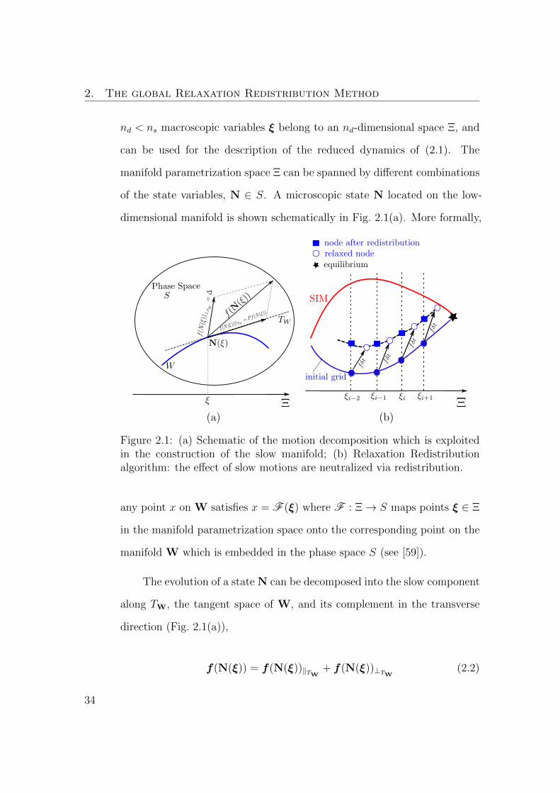
(a) (b)
Figure 2.1: (a) Schematic of the motion decomposition which is exploitedin the construction of the slow manifold; (b) Relaxation Redistributionalgorithm: the effect of slow motions are neutralized via redistribution.
any point x on W satisfies x = F (ξ) where F : Ξ→ S maps points ξ ∈ Ξ
in the manifold parametrization space onto the corresponding point on the
manifold W which is embedded in the phase space S (see [59]).
The evolution of a state N can be decomposed into the slow component
along TW, the tangent space of W, and its complement in the transverse
direction (Fig. 2.1(a)),
f(N(ξ)) = f(N(ξ))‖TW + f(N(ξ))⊥TW (2.2)
34

2.2. Slow invariant manifold: Concept and Construction
The slow and fast components are defined, respectively, as
f(N(ξ))‖TW = Pf(N(ξ)) (2.3)
f(N(ξ))⊥TW = ∆(N(ξ)) = f(N(ξ))−Pf(N(ξ)) (2.4)
in terms of an ns × ns projection matrix P and the defect of invariance
∆(N(ξ)).
By definition, W is a positively-invariant manifold if any state that is
initially on W remains on it during the subsequent time evolution. Hence,
relaxation will only proceed along the tangent space and the normal com-
ponent should be zero,
∆(N(ξ)) = 0, ξ ∈ Ξ (2.5)
Equation (2.5) is known as the invariance condition, and can be solved for
the unknown slow invariant manifold. In the method of invariant manifold
(MIM), the SIM is the stable solution of the so-called film extension of
dynamics [59],
dN(ξ)
dt= ∆(N(ξ)) (2.6)
which defines an evolutionary process guiding an initial guess for the man-
ifold towards the slow invariant manifold. In numerical realizations, mani-
folds are usually represented by a grid (discrete set of points), as proposed
in the method of invariant grid (MIG) [57]. Due to the locality of MIM
construction, we make no further distinction between manifold and grid.
35

2. The global Relaxation Redistribution Method
If the initial grid is subjected to the system dynamics, the distance
between the grid nodes shrinks and the whole grid contracts to a neighbor-
hood around the equilibrium state. The key idea of RRM is to alternate a
relaxation step with an appropriate movement that counterbalances shrink-
ing. One iteration step of RRM is shown schematically in Fig. 2.1(b). After
relaxation, the nodes of the initial grid (filled circles) evolve to different posi-
tions (open circles) and the macroscopic coordinates change. The increased
density of the grid points close to equilibrium can result in a reduction of
the grid spacing. To prevent this, the redistribution step brings the macro-
scopic coordinates ξ back to their previous values by interpolation between
the inner relaxed states and extrapolation for grid points outside the con-
tracted boundaries. The converged solution is the manifold containing all
the states for which further relaxations result in movement only along the
manifold.
In order to clarify the aforementioned notions, the singularly-perturbed
dynamical system proposed in [63] is considered with N = (x, y)T
dx
dt= 2− x− y (2.7a)
dy
dt= γ(√x− y) (2.7b)
For x(t), y(t) ∈ R, x(t) ≥ 0 and γ 1, the system evolves from any initial
condition (x0, y0) towards the fixed point at (1, 1).
For γ = 20, choosing ξ = x to parametrize the manifold and y = 1− x
as the initial grid, after a single integration step (relaxation) with δt = 0.07,
36

2.2. Slow invariant manifold: Concept and Construction
the initial grid (open squares) contracts significantly (Fig. 2.2(a), open cir-
cles). Redistribution is then applied to find the y values at the original
locations of the parameterizing macroscopic coordinates by linear interpola-
tion between relaxed states on the interior grid and linear extrapolation at
the boundary (two leftmost star symbols). The RRM converges to the slow
0 0.2 0.4 0.6 0.8 1−0.5
0
0.5
1
y
x
Initial grid1 Step Relaxation, δt = 0.071 Step RRM
0 0.2 0.4 0.6 0.8 1
−0.5
0
0.5
1
y
x
Sample Trajectories
RRM ManifoldILDM
Trajectory initialize on the RRM manifold
Trajectory initialize on the ILDM manifold
(a) (b)
Figure 2.2: (a) The effect of applying a single RRM step on the nodes ofthe initial grid; (b) comparison between ILDM manifold, RRM manifoldand sample trajectories γ = 20.
invariant manifold after 10 iterations for a tolerance of 10−4 (Fig. 2.2(b),
solid line).
The defect of invariance ∆ can be used as an indicator for the time
after which the reduced description becomes accurate. For the chosen
parametrization, the kernel of the projector P is (1, 0). P is spanned by
its image, which is the tangent subspace to the manifold, TW = imP, and
the orthogonal to the kernel. Hence,
P =
1
dydx
(1, 0) =
1 0
dydx
0
(2.8)
37

2. The global Relaxation Redistribution Method
From (2.4), the defect of invariance is then
∆ = (I − P )f =
0
−dy(ξ)dξ
(2− ξ − y(ξ)) + γ(√
ξ − y(ξ)) (2.9)
In this case, the manifold is smooth and dy(ξ)dξ
along the manifold can be
accurately approximated numerically by second-order central differences.
In order to compare the manifold and its invariance with the ILDM,
the Jacobian J of (2.7)
J =
−1 −1
γ2√x−γ
(2.10)
is needed. The symmetrized Jacobian J sym = JJT , which offers the advan-
tage of real eigenvalues, λ, and orthogonal eigenvectors, v, can be used to
define the fast and slow invariant subspaces of (2.7) [13, 64]. Let us define
the matrix V with a column partitioning given by the eigenvectors of J sym
ordered according to decreasing magnitude of the corresponding eigenval-
ues, V = (vslow,vfast) and its inverse V −1 =
(vslow, vfast
)T. For γ 1,
the ILDM manifold, yILDM , can be obtained by setting the inner product
of vfast with f [42, 64] equal to zero. Assuming that y is the intrinsic fast
variable, the approximate form of slow manifold is
y =√x. (2.11)
The ILDM manifold is plotted in Fig. 2.2(b) (dashed line) together with
38

2.2. Slow invariant manifold: Concept and Construction
several trajectories (dot-dashed lines) and the RRM manifold (solid line).
Trajectories initialized at the leftmost boundary of the ILDM (open squares)
and RRM (open circles) manifolds are also shown. In this case, the ILDM
manifold is neither invariant nor slow, except close to the steady state.
On the other hand, different solution trajectories are quickly attracted
(Fig. 2.2(b)) to the RRM manifold, which is also found to be invariant.
For the initial condition (x0, y0) = (0.1, 1.0), the temporal evolution of
the state and the Euclidean norm of ∆ for the RRM and ILDM manifolds
of system (2.7) are plotted in Fig. 2.3(a). The defect of invariance for the
0 1 2 3 4 50
0.2
0.4
0.6
0.8
1
x,y
t
0 1 2 3 4 510
−5
10−3
10−1
101
|∆|
y(t)
x(t)
|∆|RRM(t)
|∆|ILDM (t)
0 0.2 0.4 0.6 0.8 1−1
−0.5
0
0.5
1
x
y
Sample Trajectory
RRM Manifold
ILDM Manifold
(a) (b)
Figure 2.3: Analysis of ILDM and RRM manifold for (2.7). (a) Defects ofinvariance and temporal evolution of the state for a sample trajectory (b)Sample trajectory, ILDM and RRM manifolds in phase space for γ = 20.
RRM manifold is an order of magnitude lower than for ILDM, implying
that the RRM manifold is a better approximation for the SIM. As it can
be seen from Fig. 2.3(b), the trajectory is attracted to the RRM manifold
at (x, y) ' (0.4, 0.6). At this location, the defect of invariance for the RRM
manifold is less than 0.03, while for ILDM it is approximately 0.6.
39

2. The global Relaxation Redistribution Method
2.3 Chemical kinetics
Consider a homogeneous mixture of ideal gases consisting of ns species and
ne elements reacting under constant pressure p in a closed system. The
number of moles are represented by the vector N = (N1, N2, · · · , Nns)T
and the change in the chemical composition of the species, results from nr
reversible reactions between the ns reactants Mi
ns∑i=1
ν ′ikMi ns∑i=1
ν ′′ikMi, k = 1, · · · , nr (2.12)
where ν ′ik and ν ′′ik are the stoichiometric coefficients of species i in reaction k
for the reactants and products, respectively. The rate of progress of reaction
k is
qk = kfk
ns∏i=1
[Xi]ν′ik − krk
ns∏i=1
[Xi]ν′′ik , k = 1, · · · , nr (2.13)
where [Xi] denotes the molar concentration of species i and kfk and krk are
the forward and reverse rate constants having the modified Arrhenius form
kfk = AkTβk exp
(−EkRcT
)(2.14)
with Ak, βk, Ek and Rc being the pre-exponential factor, temperature ex-
ponent, activation energy and ideal gas constant, respectively. The forward
and reverse rate constants are related via the equilibrium constant, Kck(T )
krk =kfkKck
(2.15)
40

2.3. Chemical kinetics
The rate equation for species i is given by
d[Xi]
dt=
r∑k=1
(ν ′′ik − ν ′ik)qk, i = 1, · · · , ns (2.16)
Using the reactor volume V , the change in the mole number of species i can
be rewritten in the form of equation (2.1)
dN
dt=d[VX]
dt= f(N) (2.17)
The ne elemental conservation constraints can be expressed in terms of an
ne × ns elemental constraints matrix, E, as [65]
EN = ξe (2.18)
where ξe is specified by the initial composition and Eji denotes the number
of atoms of element j in species i.
In a constant pressure adiabatic system the reactions proceed at con-
stant enthalpy and the temperature evolution is governed by
dT
dt= − 1
ρcpΣnsi=1hiωiWi
where, ρ is the mixture density and Wi, hi and ωi molecular weight, enthalpy
and production/destruction rate of species i. According to the second law
of thermodynamics, the system under consideration is equipped with a con-
cave state function, the entropy S, which attains its global maximum at
equilibrium. The negative of entropy, which for ideal gases mixtures under
41

2. The global Relaxation Redistribution Method
isobaric and isenthalpic conditions takes the form [58]
G = −S = −∑ns
i=1 Xi
(si(T )−Rc ln(Xi)−Rc ln
(p
pref
))W
(2.19)
is a thermodynamic Lyapunov function for the dynamics defined by (2.17)
in terms of si, the specific entropy of species i, W =∑ns
i=1XiWi the mean
molecular weight, p and pref , the system and reference pressure; Xi =
Ni/∑ns
j=1Nj is the mole fraction of species i.
The equilibrium composition, Neq, is the solution of the constrained
minimization problem:
min G
s.t. EN = ξe(2.20)
This Lyapunov function can be exploited not only to compute the equilib-
rium, but also for the derivation of the reduced description as described in
the next section.
2.4 Construction of the reduced description
The local realization of the Relaxation Redistribution Method [58] con-
structs and tabulates SIMs with dimension nd adaptively varying in dif-
ferent regions of the phase space. Adaptation of the dimension is based on
the failure of the algorithm to converge after a fixed number of iterations,
which is taken as an indicator that the SIM dimension should be increased.
However, the computational cost associated with the manifold repre-
sentation on a grid and the retrieval of information from high-dimensional
42
2.4. Construction of the reduced description
tables imposes restrictions on the dimensionality of the slow manifold, the
target being a two- or three-dimensional table [18]. A low-dimensional SIM
is usually limited to a small neighborhood of phase space around the equilib-
rium point, leaving open the problem of its extension to cover all admissible
states [66].
In this work, the global realization of the RRM with an a priori chosen
manifold dimension is employed. In particular, an RCCE manifold, which
provides ‘good’ manifolds as discussed in the introduction, with dimension
up to three is used to define the initial SIM. The initial approximation is
subsequently refined using RRM. For regions of the phase space in the neigh-
borhood of the equilibrium, the method converges to the SIM. For states
farther away, where no SIM with the chosen dimension exists, the refined
Quasi-Equiibrium Manifold (QEM) defined below provides an accurate ex-
tension as will be shown in section 2.5. In addition to the parametrization
of the SIM, the initial RCCE manifold defines the boundaries which are
kept fixed during the application of RRM.
2.4.1 Initialization: the Quasi-Equilibrium Manifold
For systems equipped with a Lyapunov function, a reduced description can
be obtained based on the notion of the Quasi-Equilibrium Manifold (QEM)
[59] (known as Constrained Equilibrium Manifold (CEM) in the combustion
literature [44, 45]). QEM assumes that the system relaxes to equilibrium
through a sequence of quasi-equilibrium states at a rate controlled by a
set of appropriate slowly-varying constraints ξ [44, 45, 59, 67]. Since the
43

2. The global Relaxation Redistribution Method
Lyapunov function G decreases in time, a QEM can be interpreted as the
constrained minimum of G.
In addition to the elemental conservation constraints (Eq. (2.18)), QEM
imposes a priori nd linear constraints on the system state defining the slow
macroscopic variables
ξd = (Bd)N (2.21)
Bd is an nd×ns matrix with rows obtained from the coefficients of the linear
combinations of the number of moles providing the nd slow parameterizing
variables ξd. Thus, the total number of constraints amounts to nc = ne +
nd, and the QEM is the map NQEM(ξ), obtained by solving the following
constrained convex minimization problem
min G
s.t. BN = ξ(2.22)
Here, B = [E Bd] is the nc × ns constraint matrix and ξ = [ξe ξd] the
constraint vector with nc elements. The ns-dimensional state N can then be
parametrized by the nc variables ξ. For model reduction purposes, nc ns.
In closed reactive systems, the elemental mole numbers must be con-
served. Hence, EN = ξe is fixed upon definition of the fresh mixture con-
dition. The constraint matrix Bd can be selected on the basis of numerical
results of detailed solutions for similar problems, as suggested for example
in [68]. Alternatively, a suitable parametrization can be extracted using the
spectral decomposition of the Jacobian matrix evaluated at the equilibrium
44

2.4. Construction of the reduced description
point [41]. It should be pointed out that a QEM is typically neither an
invariant nor a slow manifold [67].
The choice of a good set of constraints can be challenging. In addi-
tion to intuition and the mentioned approaches, CSP analysis of detailed
simulations can aid in the selection [68]. The Level Of Importance (LOI),
which finds the species associated with the short time scales by means of a
combined species lifetime and sensitivity parameters, has also been used in
the RCCE context [69]. In general, the constraints must [70,71]
(a) be linearly independent
(b) constrained initial state should approximate the initial composition
(c) constrain global reactions in which reactants or intermediates go di-
rectly to products
(d) determine the energy and entropy of the system within experimental
accuracy.
The RCCE method, which is based on the QEM approach can be used
either as proposed originally [72–74], or in combination with other methods
[75]. The most commonly employed slowly-changing constraints are the
total number of moles (TM), the total number of radicals referred to active
valence (AV), and free oxygen (FO), which refers to the reactions where the
O-O bond is broken [67]. These RCCE linear constraints for hydrogen/air
combustion are specified in Table 2.1. The RCCE manifold is unique and
infinitely differentiable, and can be used even for states far from equilibrium
[65, 70]. In this chapter, we exploit the QEM notion only to construct the
45

2. The global Relaxation Redistribution Method
Table 2.1: Matrix Bd for the H2/air mixture
Reduced variable H2 N2 H O OH O2 H2O HO2 H2O2
ξd1=TM 1 1 1 1 1 1 1 1 1ξd2=AV 0 0 1 2 1 0 0 0 0ξd3=FO 0 0 0 1 1 0 1 0 0
initial approximation of the SIM and to define the manifold boundaries.
2.4.2 The global Relaxation Redistribution algorithm
As discussed in section 2.2, the boundaries of the initial grid shrink during
relaxation. In the local RRM, reconstruction of the boundary points by
re-stretching the relaxed grid to the fixed boundaries is done by linear ex-
trapolation. However, such an approach cannot always guarantee physically
meaningful values for the species concentrations. In order to avoid this dif-
ficulty, the boundary of the SIM can be fixed to the initial guess provided
by the QEM, and the RRM procedure is applied only to the interior grid
points.
The embarrassingly simple steps for the computation of the global man-
ifold proceed as follows:
1. Choose the manifold dimension nd and select the parameterizing vari-
ables ξi
2. Construct the nd-dimensional QEM, NQEM(ξd), by solving the min-
imization problem (2.22). This manifold corresponds to construct-
ing the initial grid indicated by the solid line with filled circles in
Fig. 2.1(b).
46
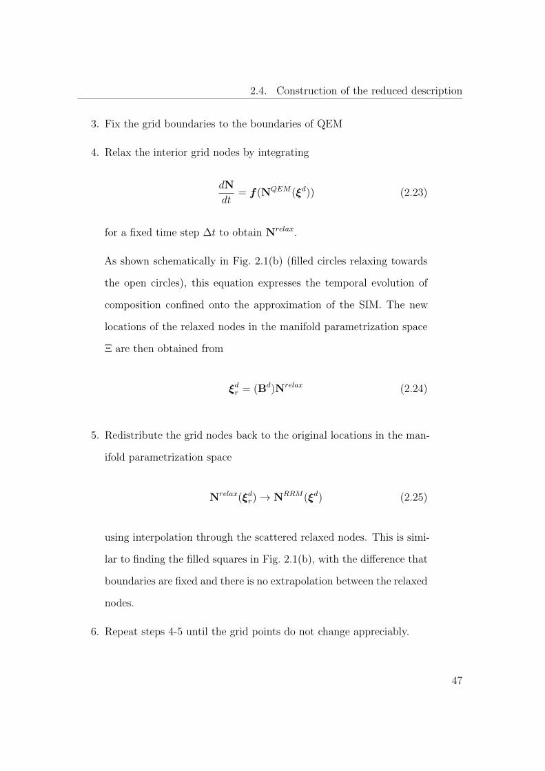
2.4. Construction of the reduced description
3. Fix the grid boundaries to the boundaries of QEM
4. Relax the interior grid nodes by integrating
dN
dt= f(NQEM(ξd)) (2.23)
for a fixed time step ∆t to obtain Nrelax.
As shown schematically in Fig. 2.1(b) (filled circles relaxing towards
the open circles), this equation expresses the temporal evolution of
composition confined onto the approximation of the SIM. The new
locations of the relaxed nodes in the manifold parametrization space
Ξ are then obtained from
ξdr = (Bd)Nrelax (2.24)
5. Redistribute the grid nodes back to the original locations in the man-
ifold parametrization space
Nrelax(ξdr)→ NRRM(ξd) (2.25)
using interpolation through the scattered relaxed nodes. This is simi-
lar to finding the filled squares in Fig. 2.1(b), with the difference that
boundaries are fixed and there is no extrapolation between the relaxed
nodes.
6. Repeat steps 4-5 until the grid points do not change appreciably.
47

2. The global Relaxation Redistribution Method
It should be pointed out that the reduced descriptions obtained by this
algorithm are closely related to the ICE-PIC approach suggested by Ren et
al. in [46], as both procedures construct invariant manifolds forced to pass
through the fixed boundary points (QEM boundary points).
2.4.3 Rate equations for the slow variables
Once the slow invariant manifold is constructed, the temporal evolution of
the reduced system along the SIM can be recast in the following general
form in terms of the macroscopic slow variables ξd chosen to parametrize
the SIM:
dξd
dt= (Bd)Pf(NRRM(ξd)) (2.26)
If the slow invariant manifold is known accurately, the vector field f is per-
fectly aligned with the manifold’s tangent space and the state would never
depart from the manifold. In most computational applications of practical
interest, however, SIM approximations with different levels of accuracy are
employed, and the chosen parametrization cannot completely decouple the
fast and slow components. In these cases, (Bd)f does not lie on the tangent
space of the SIM and a projector P is needed to bring the state back to the
manifold.
Different projectors have been proposed in the literature. The ILDM
projector recovers the fast subspace to leading order [76], and the kernel
of the projector is constructed using the fastest eigenvectors of the local
Jacobian. Higher-order approximations can be constructed using the CSP
basis vectors. Details on the ILDM and CSP projectors can be found in
48

2.4. Construction of the reduced description
[42, 77]. Another option for P is the thermodynamic projector [78], which
can be constructed on the basis of the local tangent space to the SIM and
the derivatives of a thermodynamic Lyapunov function (2.19) [79].
In the classical RCCE method, it is assumed that states of the system
always remain on the QEM and the rate equations for the slow parame-
terizing variables is close to the tangent space of the manifold [67]. The
ns-dimensional composition space is decomposed into the nd-dimensional
represented subspace spanned by the rows of Bd and its orthogonal comple-
ment, the unrepresented subspace of dimension ns − nd. The projection is
illustrated schematically in Fig. 2.4. The projection matrix then becomes
the ns×ns-dimensional identity matrix which implies that the rate of change
in the unrepresented subspace is negligible. Therefore we rely upon the fact
that fast motions are expected to mostly occur in the null space of the
Bd matrix. The same approach was used in the applications of the results
section. For a more detailed analysis of this projector see [75].
The following steps describe the implementation of reduced chemistry
in a reacting flow simulation: (a) From the specified composition at time
tn, Nn = N(tn), and the thermodynamic conditions, the values for the
parameterizing variables can be found using equation (2.21),
(Bd)Nn = ξdn (2.27)
(b) The rate equations (2.26) for ξd, are advanced in time to find ξdn+1,
where NRRMn are the projected values of N(tn) on the SIM.
49

2. The global Relaxation Redistribution Method
Figure 2.4: Project in the unrepresented subspace of RRM manifold. Theprojection is same as classical RCCE [67]
The reduced model can be tabulated in terms of either the reduced
state NRRM or of the projected right hand side of the evolution equations
(Bd)f(NRRM). In the former case, interpolation of the tabulated data
is used to retrieve the composition vector corresponding to ξdn+1. In the
latter, the right hand side of (2.26) is obtained directly to proceed with the
integration of the reduced system and the compositions can be obtained
separately in a post-processing step.
The overall computational cost for the integration of the full system of
ns differential equations is thus replaced by the cost of integrating nd differ-
ential equations and of interpolation. The following practical issues should
be pointed out: (i) Choosing the appropriate constraints with respect to the
initial composition is important. The kernel of Bd should not be spanned
by the f(NRRMn (ξd)) vector, since in that case dξd
dtbecomes zero and there is
no temporal evolution of ξd; (ii) Interpolation can affect the result strongly
50

2.5. Validation and discussion
as shown in [80]. This effect can be controlled by refining the table and/or
using appropriate interpolation methods, albeit at higher computational
cost; (iii) By construction, the approach presented here guarantees that the
equilibrium will be accurately captured by the reduced description. This
appears to not always be the case with reduced mechanisms proposed in
the literature; (iv) In problems like the ignition delay time considered in the
next section, the projection of the initial state on the manifold is crucial
for the comparison with the prediction of the detailed reaction mechanism.
In the literature, the comparison is often made by taking the initial state
to lie on the manifold. In the auto-ignition validation of the next section
good results are obtained by comparing the detailed solution with those ob-
tained by projecting the initial state on the manifold using the constrained
equilibrium assumption.
2.5 Validation and discussion
2.5.1 Auto-ignition of homogeneous mixtures
The global RRM method is applied to a homogeneous H2/air mixture using
the detailed reaction mechanism of Li et al. [17]. (ns = 9 species and 21
reactions) at atmospheric pressure and different initial temperatures T0.
The initial reactant composition is that of a stoichiometric mixture
(N0H2
= 1.0, N0O2
= 0.5 and N0N2
= 1.881 mole), while the remaining species
are assigned the chemically insignificant positive values N = 10−12 mole to
ensure strictly positive species compositions at the constrained equilibrium
51

2. The global Relaxation Redistribution Method
state and guarantee the existence and uniqueness of the solution to the
minimization problem (2.22) [67].
The equilibrium point (steady state) can be computed by minimizing
the Gibbs function under constant pressure and enthalpy. Then, the ini-
tial and equilibrium states are projected on the manifold parametrization
space, Ξ, using (2.21). Different combinations of constraints for hydrogen
combustion have been investigated in the literature [67, 70]. The TM and
AV constraints (Table 2.1) have been found to give better agreement with
respect to ignition delay times for a wide range of thermodynamic condi-
tions and are chosen for the ξ parameterization. Starting from a sufficiently
large range in the parametrization space that contains the initial and steady
states, the CEQ code [81,82] is used for the construction of the RCCE-based
initial manifold as discussed in section 2.4.2. The code computes the con-
strained equilibrium state by minimizing the Gibbs function under fixed
pressure and enthalpy; the projection of the computed initial manifold on
Ξ is shown in Fig. 2.5. The boundary nodes are then fixed, and the RRM
procedure is applied to the interior nodes. For the redistribution step, the
linear Shepard method implemented in the SHEPPACK package [83] is used
for interpolation,
NRRM(ξd) =
∑ngpk=1 αk(ξ
d)Nrelax(ξdr)∑ngpk=1 αk(ξ
d)(2.28)
where ngp is the total number of grid points and the weights αk(ξd) are
52

2.5. Validation and discussion
2.8 3 3.2 3.4 3.6 3.80
0.2
0.4
0.6
0.8
1
1.2
1.4
1.6
ξ 2
ξ1
Equilibrium
Fresh Mixture
Figure 2.5: Projection of manifold (grid) onto Ξ. The initial grid shouldcontain both the fresh mixture and equilibrium point, and extend in themanifold parametrization space as far as the QEM convex minimizationcalculations converge.
defined as
αk(ξd) =
1
‖ξd − ξd(k)r ‖2
2
(2.29)
For initial temperature T0 = 1500 K, the two-dimensional RCCE and global
RRM manifolds for selected species are plotted in Fig. 2.6 together with the
trajectory obtained using the detailed mechanism (thick solid line). For the
major species, the global RRM manifold brings only a slight improvement
over the RCCE manifold, while for HO2 and H2O2 the improvement is
significant. As it can be seen in Fig. 2.6, the RCCE manifold is not invariant.
This is more clearly seen in the temporal evolution of the temperature and
53

2. The global Relaxation Redistribution Method
2.83
3.23.4
3.63.8
0
0.5
10
0.2
0.4
0.6
0.8
1
ξ1
RCCE
ξ2
NH
2
2.83
3.23.4
3.63.8
0
0.5
10
0.2
0.4
0.6
0.8
1
ξ1
RRM
ξ2
NH
2
(a)
2.53
3.54
0
0.5
10
0.05
0.1
0.15
0.2
0.25
ξ1
RCCE
ξ2
NO
2.53
3.54
0
0.5
10
0.05
0.1
0.15
0.2
0.25
ξ1
RRM
ξ2
NO
(b)
2.8 3 3.2 3.4 3.6 3.8
0
0.5
10
0.05
0.1
0.15
0.2
ξ1
RCCE
ξ2
NOH
2.8 3 3.2 3.4 3.6 3.8
0
0.5
10
0.05
0.1
0.15
0.2
ξ1
RRM
ξ2
NOH
(c)
2.8 3 3.2 3.4 3.6 3.80
0.5
1
0
1
2
3
x 10−4
RCCE
ξ1ξ2
NHO
2
2.8 3 3.2 3.4 3.6 3.80
0.5
1
0
0.2
0.4
0.6
0.8
1
x 10−3
RRM
ξ1ξ2
NHO
2
(d)
Figure 2.6: Comparison of the RCCE (left column) and RRM (right column)manifolds for T0 = 1500 K. (: fresh mixture; ?: equilibrium point; −:detailed kinetics trajectory).
54

2.5. Validation and discussion
species mass fractions, plotted in Fig. 2.7. Good agreement is found with
the detailed description for the temperature and major reactants as well as
the radicals with high enough concentration. Far away from equilibrium,
the RCCE manifold strongly underpredicts the concentration of HO2 and
H2O2.
0 0.5 1 1.5
x 10−4
1500
2000
2500
3000
T[K
]
t [s]
Detailed
RCCE TM+AV
RRM 2D
0 0.5 1 1.5
x 10−4
0
0.01
0.02
0.03
YH
2
t [s]0 0.5 1 1.5
x 10−4
0
2
4
6x 10
−3
YH
t [s]
0 0.5 1 1.5
x 10−4
−0.01
0
0.01
0.02
0.03
YO
t [s]0 0.5 1 1.5
x 10−4
0
0.01
0.02
0.03
YOH
t [s]0 0.5 1 1.5
x 10−4
0
0.05
0.1
0.15
0.2
0.25
YO
2
t [s]
0 0.5 1 1.5
x 10−4
0
0.05
0.1
0.15
0.2
YH
2O
t [s]0 0.5 1 1.5
x 10−4
0
2
4
6x 10
−5
YHO
2
t [s]0 0.5 1 1.5
x 10−4
0
0.5
1
1.5x 10
−5
YH
2O
2
t [s]
Figure 2.7: Time histories of the temperature and species mass fractionsfor H2/air autoignition with unburnt temperature T0 = 1500K.
The time history of the weighted root mean square norm as used
for error estimation in [84] of the defect of invariance vector is plotted
in Fig. 2.8(a) together with the temperature profiles computed using the
detailed and reduced descriptions. After 40µs, the defect drops below 10−4
55

2. The global Relaxation Redistribution Method
and the detailed and reduced models are in good agreement. This illustrates
that the defect of invariance is a convenient indicator of the accuracy of the
reduced description. During the initial transient, a higher-dimensional man-
ifold should be used.
The number of right hand side function evaluations nfe during integra-
tion can be used as an indicator for the stiffness. Figure 2.8(b) shows the
temperature and nfe obtained by using the stiff ODE integrator DVODE [84]
with an output time step δt = 10−5 (the integrator adapts the time step
during integration from time t to t + dt). The initial composition for the
detailed mechanism was the stoichiometric mixture, while for the reduced
description its projection on the RRM manifold was used. With the excep-
tion of a single time instant close to ignition, nfe is lower for the reduced
model during the whole integration interval.
At a lower initial temperature T0 = 1000 K, the 2-D manifold can no
longer provide an accurate reduced description (Fig. 2.9). The construction
of a 3-D slow manifold is straightforward starting from an initial manifold
constructed using all constraints of Table 2.1. The results obtained with
RCCE with two (open squares) and three (open circles) constraints, the
RRM 2-D (dot-dashed line) and 3-D (dashed line) manifolds are compared
with the detailed evolution (solid line) in Fig. 2.9. While the 3-D RCCE
manifold results in small improvement, the increase in the manifold dimen-
sion of the RRM manifold leads to very good agreement with respect to the
prediction accuracy of the ignition delay time and the temporal evolution
of temperature and species, with the exception of the YH2O2 profile which
56

2.5. Validation and discussion
0 0.5 1 1.5
x 10−4
1400
1600
1800
2000
2200
2400
2600
2800
3000
T[K
]
0 0.1 0.2 0.3 0.4 0.5 0.6 0.7 0.8 0.9 1 1.1 1.2 1.3 1.4
x 10−4
10−10
10−8
10−6
10−4
10−2
100
t [s]
‖∆
‖ weig
hted
RRM 2D
Detailed
∆10
20
30
40
50
60
70
80
nfe
Detailed system nfe
Reduced system nfe
0.0 5.0×10⁻⁵
1.0×10⁻⁴
1.5×10⁻⁴
2.0×10⁻⁴
t [s]
1500
2000
2500
3000
T [
K]
Detailed system temperature
Reduced system temperature
(a) (b)
Figure 2.8: (a) Comparison of the temperature profiles obtained with thedetailed and the reduced 2-D RRM description and evolution of the normof the defect of invariance for T0 = 1500 K; (b) Comparison of temperatureevolution and number of source term evaluations nfe obtained with thedetailed mechanism and the reduced 2-D RRM description at T0 = 1500 K.
displays a noticeable deviation from the detailed mechanism profile. The
ignition delay times, τig, defined as the time corresponding to the inflection
point of the temperate profile are summarized in Table 2.2. The magnitude
Table 2.2: Comparison of ignition delay times deduced from detailed andreduced models.
Method τig(sec)Detailed 0.000213
RCCE TM+AV 0.000169RCCE TM+AV+FO 0.000178
RRM 2D 0.000170RRM 3D 0.000207
of the real part of the six non-trivial eigenvalues of the Jacobian matrix
during the temporal evolution for T0 = 1000 K and T0 = 1500 K are re-
ported in Fig. 2.10. The absolute value of the inverse of the eigenvalues
57

2. The global Relaxation Redistribution Method
0 1 2 3 4
x 10−4
1000
1500
2000
2500
3000T[K
]
t [s]
RCCE TM+AV+FO
RCCE TM+AV
RRM 2D
RRM 3D
Detailed
0 1 2 3 4
x 10−4
0
0.005
0.01
0.015
0.02
0.025
0.03
YH
2
t [s]0 1 2 3 4
x 10−4
0
1
2
3
4
5
6x 10
−3
YH
t [s]
0 1 2 3 4
x 10−4
0
0.005
0.01
0.015
YO
t [s]0 1 2 3 4
x 10−4
0
0.005
0.01
0.015
0.02
0.025
0.03
YOH
t [s]0 1 2 3 4
x 10−4
0
0.05
0.1
0.15
0.2
0.25
YO
2
t [s]
0 1 2 3 4
x 10−4
0
0.05
0.1
0.15
0.2
0.25
YH
2O
t [s]0 1 2 3 4
x 10−4
0
1
2x 10
−4
YHO
2
t [s]0 1 2 3 4
x 10−4
10−8
10−6
10−4
10−2
YH
2O
2
t [s]
Figure 2.9: Temperature and species mass fractions as the function of timefor H2/air auto-ignition, T0 = 1000 K. Detailed, RCCE with 2 Constraints,RCCE with 3 Constraints, RRM 2D manifold, RRM 3D manifold are com-pared.
determine the time scales of the chemical modes and the ratio λf/λs of
the most to the less negative eigenvalues, an estimation for stiffness. For
T0 = 1000 K, the gap is λf/λs ' 8.5× 10⁸, while for T0 = 1500K the ratio
becomes λf/λs ' 5.6 × 10⁵, reflecting the higher stiffness at lower temper-
atures. Eigenvalues with positive real part indicating explosive behavior
were found initially in both cases and time intervals where the eigenvalues
cross and become complex pairs were observed during the evolution from
the initial to the equilibrium state. Manifolds of higher dimensions would
58

2.5. Validation and discussion
0 1×10⁻⁴
2×10⁻⁴
3×10⁻⁴
4×10⁻⁴
t [s]
10-3
100
103
106
109
| λ
|
[
s-1 ]
λ1=λ
f
λ2
λ3
λ4
λ5
λ6=λ
s
0 5×10⁻⁵
1×10⁻⁴
t [s]
103
106
109
| λ
| [
s-1 ]
λ1=λ
f
λ2
λ3
λ4
λ5
λ6=λ
s
(a) (b)
Figure 2.10: Temporal evolution of the six non-trivial eigenvalues of theJacobian along the solution trajectory: (a) T0 = 1000 K, (b) T0 = 1500 K.
be needed to capture more accurately the reduced dynamics in these inter-
vals, as was done in the adaptive version of RRM [58]. Careful examination
of Fig. 2.10 for T0 = 1500 K reveals that eigenvalue crossings correspond to
jumps in (a) the defect of invariance vector (Fig. 2.8(a)) and (b) the num-
ber of source term evaluations nfe (Fig. 2.8(b)). The effect of eigenvalues
crossing on the quality of reduced model is discussed in [85]. It nevertheless
appears that these short intervals do not affect the quality of the manifold
significantly.
2.5.2 Premixed laminar flame
The steady, atmospheric, adiabatic, one-dimensional laminar premixed flame
of a stoichiometric hydrogen/air mixture and multi-component transport
properties was considered in order to study the ability of the 2-D RRM
manifold constructed from the homogeneous auto-ignition of an unburnt
mixture at Tu = 700 K to reconstruct the unrepresented variables in a case
where transport phenomena play a dominant role. A similar procedure was
59
2. The global Relaxation Redistribution Method
used for the validation of the ICE-PIC manifold by Ren el al. [46].
In this case, the manifold parametrization becomes important since
in the general case of non-unity Lewis numbers it is difficult to solve the
partial differential equations even when the parameterizing variables are lin-
ear combinations of the original variables [86]. Here, the quasi-equilibrium
manifold was constructed using the mole fractions of H2O and H2 as slow
constraints (ξ1 = XH2O and ξ2 = XH2). The RRM refinement process was
applied starting from the QEM to find the global two dimensional manifold
for Tu = 700 K. The species concentrations as a function of the distance,
0 0.2 0.4 0.6 0.8 10
0.1
0.2
0.3
0.4
XH
2
x [cm]
0 0.2 0.4 0.6 0.8 10
0.05
0.1
0.15
0.2
XO
2
x [cm]
0 0.2 0.4 0.6 0.8 10
0.02
0.04
0.06
0.08
XH
x [cm]
0 0.2 0.4 0.6 0.8 10
0.005
0.01
0.015
XO
x [cm]0 0.2 0.4 0.6 0.8 1
0
0.005
0.01
0.015
0.02
0.025
XOH
x [cm]
0 0.2 0.4 0.6 0.8 10
0.1
0.2
0.3
0.4
XH
2O
x [cm]0 0.2 0.4 0.6 0.8 1
10−10
10−8
10−6
10−4
10−2
XHO
2
x [cm]0 0.2 0.4 0.6 0.8 1
10−10
10−5
100
XH
2O
2
x [cm]
0 0.2 0.4 0.6 0.8 1500
1000
1500
2000
2500
3000
T[K
]
x [cm]
Detailed
RRM 2D
Figure 2.11: Comparison of the temperature and species mole fractions pro-files computed by PREMIX (lines) and reconstructed using the 2-D RRMmanifold (symbols) for unburnt mixture at T0 = 700 K.
60

2.6. Summary and Conclusions
x, is computed using PREMIX from the CHEMKIN application suite [87].
The local values of XH2 and XH2O from the detailed chemistry 1-D flame
structure were used to reconstruct the remaining species using the RRM
manifold. The agreement for the major species and temperature between
the detailed solution and the reconstruction is excellent (Fig. 2.11). The
largest differences are observed for the H2O2 species and they can be mainly
attributed to the incorrectly predicted value of QEM at the“cold”(unburned
mixture) boundary. In addition to low dimensionality effects, molecular dif-
fusion in laminar flames can drive the compositions away from the manifold,
potentially contributing in the differences observed in the O and H radicals
profiles. Similar observations are reported in the literature, where different
methods of projecting the diffusion term onto the manifold were studied
(see, for example, [76,88])
2.6 Summary and Conclusions
In this chapter we presented an algorithm based on the Relaxation Redistri-
bution Method (RRM) for the construction of the Slow Invariant Manifold
(SIM) of an a priori chosen dimension which covers a large fraction of the
admissible composition space that includes the equilibrium as well as the
initial state.
The manifold parametrization and boundaries are determined with
the help of the Rate Controlled Constrained Equilibrium (RCCE) method,
which also provides the initial guess for the SIM. The guess is iteratively
refined and the converged manifold is tabulated. The method is easy to
61

2. The global Relaxation Redistribution Method
implement and robust to use for the construction of reduced manifolds of
high dimensionality, which were found to be invariant over extended regions
of the admissible space. A criterion based on the departure from invariance
is proposed to find the region over which the reduced description is valid.
The accuracy of the method was assessed by comparing trajectories for
auto-ignition calculations of homogeneous H2/air mixtures at different ini-
tial temperatures T0. At T0 = 1500 K, a 2-D manifold is found to capture
accurately both the ignition delay time and the temporal evolution of all
the species and shows significant improvement with respect to the low con-
centration species (HO2 and H2O2) compared to an RCCE manifold. At
T0=1000 K, a 3-D manifold is needed to reproduce accurately the detailed
dynamics with the exception of the pre-ignition profiles of H2O2 while, con-
structing the 3-D manifold is barely reported in chemical kinetics reduction
literature.
The significant reduction in the number of source term evaluations
indicates that the reduced descriptions are less stiff. However, similar to
all other reduction methods based on tabulation, fast table searching and
interpolation algorithms are essential for the overall efficiency of the reduced
scheme.
The 2-D RRM manifold can reconstruct the laminar premixed flame
structure fairly accurately compared with the results obtained with the
detailed mechanism, indicating that it can be used in multidimensional
simulations where transport properties play a dominant role.
62

Chapter 3
Spectral Quasi Equilibrium
Manifold
3.1 Introduction
Entropy and entropy production are two well-studied thermodynamic func-
tions, which can be more informative than the original system dynamics.
Entropy can be considered as a Lyapunov function of a closed system which
can create a logical bridge between thermodynamics and dynamical sys-
tem analysis. For example, trajectories with minimal entropy production
have been considered as candidates for one-dimensional slow manifolds [47].
On the other hand, it can be assumed that physical and chemical kinetic
systems evolve in the vicinity of Quasi Equilibrium States (QES), where
entropy is maximized under certain constraints [59].
In physical kinetic, the works on hydrodynamic limits of the Boltz-
mann equation is an example of reducing the infinite system of moments of
particle distribution to a smaller number of representative moments. The
63
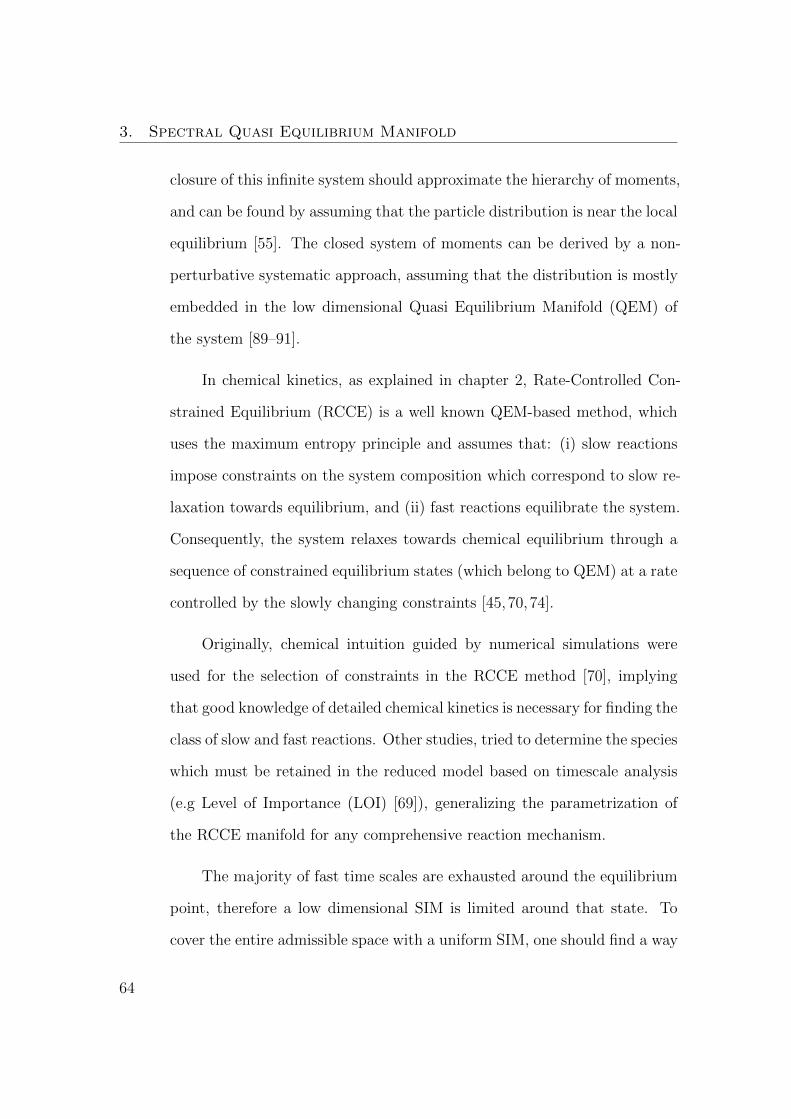
3. Spectral Quasi Equilibrium Manifold
closure of this infinite system should approximate the hierarchy of moments,
and can be found by assuming that the particle distribution is near the local
equilibrium [55]. The closed system of moments can be derived by a non-
perturbative systematic approach, assuming that the distribution is mostly
embedded in the low dimensional Quasi Equilibrium Manifold (QEM) of
the system [89–91].
In chemical kinetics, as explained in chapter 2, Rate-Controlled Con-
strained Equilibrium (RCCE) is a well known QEM-based method, which
uses the maximum entropy principle and assumes that: (i) slow reactions
impose constraints on the system composition which correspond to slow re-
laxation towards equilibrium, and (ii) fast reactions equilibrate the system.
Consequently, the system relaxes towards chemical equilibrium through a
sequence of constrained equilibrium states (which belong to QEM) at a rate
controlled by the slowly changing constraints [45,70,74].
Originally, chemical intuition guided by numerical simulations were
used for the selection of constraints in the RCCE method [70], implying
that good knowledge of detailed chemical kinetics is necessary for finding the
class of slow and fast reactions. Other studies, tried to determine the species
which must be retained in the reduced model based on timescale analysis
(e.g Level of Importance (LOI) [69]), generalizing the parametrization of
the RCCE manifold for any comprehensive reaction mechanism.
The majority of fast time scales are exhausted around the equilibrium
point, therefore a low dimensional SIM is limited around that state. To
cover the entire admissible space with a uniform SIM, one should find a way
64

3.1. Introduction
to extend the manifold. The quasi-equilibrium manifold has been proposed
in the literature both for species reconstruction (manifold extension) for
the states far from equilibrium and for obtaining the manifold boundaries
[46,92].
In the spirit of the QEM, the Spectral Quasi Equilibrium Manifold
(SQEM) has been employed as an initial manifold which is subsequently
refined towards the SIM [13,41,93]. The method has been applied to small
systems of ODEs (up to hydrogen combustion which is effectively six di-
mensional). In this chapter, the ability of the spectral quasi-equilibrium
method to provide general constraints, which do not resort on intuition, is
investigated and applied for the construction of quasi-equilibrium manifolds
for hydrogen, syngas and methane combustion.
The method is first validated through the two-dimensional Michaelis-
Menten kinetic scheme, where the quality of the reduction is discussed and
related to the temporal evolution and the gap in the spectra of eigenvalues
and Lyapunov exponents. In addition to simple enzyme kinetics, the ability
of the method is explored for detailed combustion mechanisms. The tem-
poral evolution of temperature and species concentrations deduced from re-
duced and detailed models are used as indicators of the quality of reduction,
showing the potential of SQEM for the reconstruction of species concentra-
tions and temperature profiles. The comparison also shows that the spectral
constraints show better agreement with the detailed model compared to the
classical RCCE constraints.
65

3. Spectral Quasi Equilibrium Manifold
3.2 Equilibrium and quasi-equilibrium
Lyapunov functions can be more informative and fundamental than the
original system (2.17) itself. For example, even for dynamical systems whose
detailed behavior is unpredictable, Lyapunov functions can be used as the
quantity, measuring how “complex” or unpredictable, the motion is [94–96].
The entropy S, as the distinguished Lyapunov function, which mono-
tonically increases along all possible trajectories in phase space is widely
used in physical and chemical kinetics to describe different features of the
system. Because entropy is increasing monotonically through the relaxation,
the global equilibrium state corresponds to the global maximum entropy
state. Therefore, instead of integrating the system for long (more formally
infinite) time, one can find the equilibrium via maximization of the entropy.
The equilibrium composition, N eq, is the constrained minimum of
the thermodynamic potential G(N , p, T ) (Eq. (2.20)). The concept of the
Quasi-Equilibrium Manifold stems from Grad’s approximation for the clo-
sure of the system of moments. “Of course, to any degree of approximation,
these solutions approximate to only a small part of the manifold of solutions
of the Boltzmann equation [55].” The QEM is the loci of states NQEM , ob-
tained by solving the following constrained optimization problem,
max S
s.t. ξ = G (N )(3.1)
where, ξ = G (N ) is the set of selected moments and the map G −1 : ξ −→N
66

3.2. Equilibrium and quasi-equilibrium
is a closure assumption [59]. The system of equations (3.1) is the same as
system (2.22). As we know, the global equilibrium is the state where all
processes are relaxed. We consider the case where only fast processes of
the system are relaxed. This Quasi Equilibrium State (QES) can be found
similarly by maximizing the entropy but under additional constraints on
the original dynamics (see Eq. (2.21)).
3.2.1 Spectral quasi-equilibrium manifold
The general form of the constraint matrix Bd in (2.21) reads
Bd =
v1
...
vnd
(3.2)
where vi is a ns-dimensional vector defining the ith constraint. A different
set of constraints for the construction of the pertinent quasi-equilibrium was
proposed by Gorban and Karlin [13] based on the left eigenvectors of the
Jacobian system at equilibrium,
Jeqij =
[∂f(Ni)
∂Nj
]N=Neq
(3.3)
where f for the case of homogeneous reactor is introduced in (2.17).
Let us define the matrix V eq with a column partitioning given by the
right eigenvectors of J eq ordered according to decreasing values of the cor-
67

3. Spectral Quasi Equilibrium Manifold
responding eigenvalues, V eq = [veqslow, veqfast] and its inverse
V eq−1
=(veqslow,v
eqfast
)T. (3.4)
The veqslow at equilibrium can be used as the vectors which define the di-
rection of slow processes leading the relaxation towards the final state, so
that the rows of Bd in Eq. (3.2) are the first nd slow left eigenvectors at
equilibrium.
The construction of SQEM is local, hence, instead of constructing and
tabulating the manifold, the subsequent states of detailed models can be
compared with the evolution of spectral quasi-equilibrium states (SQES).
Before considering application of the above SQEM to combustion mecha-
nisms, let us consider a simple example.
3.2.1.1 Example: Reversible Michaelis-Menten mechanism
The reversible Michaelis-Menten mechanism is a simple enzyme reaction
where enzyme E binds to a substrate S to form the intermediate complex
ES which is then converted into the product P , releasing the free enzyme
E [97]
S + Ekf1−−−−kr1
ESkcat−−−−kr2
E + P (3.5)
Here, kf1, kcat and kr1, kr2 are respectively the rate constants of the forward
and reverse reactions. The system of differential equations describing the
68

3.2. Equilibrium and quasi-equilibrium
temporal evolution of species concentrations is
d[S]
dt= −kf1[S][E] + kr1[ES] (3.6a)
d[E]
dt= −kf1[S][E] + kr1[ES] + kcat[ES]− kr2[E][P] (3.6b)
d[ES]
dt= kf1[S][E]− kr1[ES]− kcat[ES] + kr2[E][P] (3.6c)
d[P]
dt= kcat[ES]− kr2[E][P] (3.6d)
where [Xi] denotes the molar concentration of species i. In the absence of
an analytical solution, two approaches, the quasi-equilibrium approximation
and the steady-state assumption, have been used in the literature to find
an expression for the rate of the catalytic step. The Michaelis-Menten
equilibrium analysis is valid if the substrate reaches equilibrium on a much
faster timescale than the product is formed [97], i.e.
kcat
kr1 1 (3.7)
The geometrical picture of the phase space evolution can be found in [98,99].
The system (3.6) is constrained by two constants for the total enzyme
and total substrate,
[E + ES] = ξe1 (3.8a)
[S + ES + P] = ξe2 (3.8b)
69
3. Spectral Quasi Equilibrium Manifold
which can be recast in the form (2.18) with E =
0 1 1 0
1 0 1 1
. The nonlin-
ear system (3.6) is therefore effectively two-dimensional. The phase portrait
for ξe1 = 1.0 and different reactions rates are shown in Fig. 3.1 where the pos-
itive semiorbits⋃t≥0 f(N (t)) for different initial conditions are projected
on the two-dimensional [S]× [ES] plane. It can be seen that after short tran-
0 0.2 0.4 0.6 0.8 1
[S]
0
0.2
0.4
0.6
0.8
1
[ES
]
t = 0.1
t = 0.2
t = 0.4
t = 0.3
t = 1.0t = 2.0
t = 4.0
t = 6.0t =
10
.0
t =
20
.0
0 0.2 0.4 0.6 0.8 1
[S]
0
0.2
0.4
0.6
0.8
1
[ES
]
t = 0.01
t = 0.03
t = 0.06
t = 0.2
t = 1.06
t = 1.68
t = 2.54
t = 4
t = 1
0
0 0.2 0.4 0.6 0.8 1
[S]
0
0.2
0.4
0.6
0.8
1
[ES
]
t = 0.001
t = 0.003
t = 0.007
t = 0.073
t = 0.48
t = 1.0
t = 2
.4
t = 3
.8
t = 8
.5
(a) (b) (c)
Figure 3.1: The phase portrait in [S] × [ES] space for Michaelis-Mentenmechanism with ξe1 = 1.0, kcat = 1.0 and kr2 = 10−5 (a) k1f = k1r = 1, (b)k1f = k1r = 10, (c) k1f = k1r = 100; Dashed line: sample trajectories, solidline: slow manifold, circles: discrete times for selected trajectories.
sients trajectories (dashed lines) are attracted to a one-dimensional mani-
fold (thick solid line) and then relax towards the zero-dimensional manifold
(equilibrium point). For the trajectory initialized with [ES]0 = [P]0 = 0 and
[S]0 = [E]0 = 1.0, the corresponding discrete time instants are also marked
for all cases in Fig. 3.1. The decrease in kcatkr1
ratio results in faster attraction
to the low dimensional manifolds.
Gorban and Shahzad [100] proposed G = −Σ4i=1[Xi]ln([Xi]/[Xi]
eq)−1
as a Lyapunov function for this mechanism. As discussed before, for the
system of ODEs (3.6) the spectral quasi-equilibrium states, can be found by
70

3.2. Equilibrium and quasi-equilibrium
solving the convex optimization problem (2.22). In this case the constraint
matrix is one dimensional, and it is taken to be equal to the slowest left
eigenvector at equilibrium, [Bd]1×4 = veqslow, hence, [B]3×4 = [E;Bd].
For the chosen trajectory ([ES]0 = [P]0 = 0 and [S]0 = [E]0 = 1.0), the
SQESs are compared with the detailed solution in Figs. 3.2, 3.3 and 3.4;
the evolution of the eigenvalues, λ and the Lyapunov exponents [101],
Λ(N , δN ) = limT→∞
(1/T ) log |(DNfT )δN |
computed using the algorithm of [102], are also presented along the trajec-
tory. The eigenvalues can identify the timescale gap where the trajectory
is close to the slow manifold while Lyapunov exponents are providing more
accurate information about the spectral gap in nonlinear dynamics even far
from slow manifolds [103].
0 5 10 15 200
0.2
0.4
0.6
0.8
1
[S]
0 5 10 15 20
0.8
0.85
0.9
0.95
1
1.05
[E]
0 5 10 15 20
time
0
0.05
0.1
0.15
0.2
0.25
[ES]
0 5 10 15 20
time
0
0.2
0.4
0.6
0.8
1
[P]
0 5 10 15 20-3
-2.5
-2
-1.5
-1
-0.5
0
Λ
0 5 10 15 20
time
-4
-3.5
-3
-2.5
-2
-1.5
-1
-0.5
0
λ
(a) (b)
Figure 3.2: The sample semiorbit for k1f = k1r = kcat = 1.0 and kr2 = 10−5.(a) Comparison between the profiles of concentration of species deducedfrom the detailed (solid lines) and the reduced SQEM description (symbols);(b) evolution of the Lyapunov exponents and the eigenvalues of the system;
71
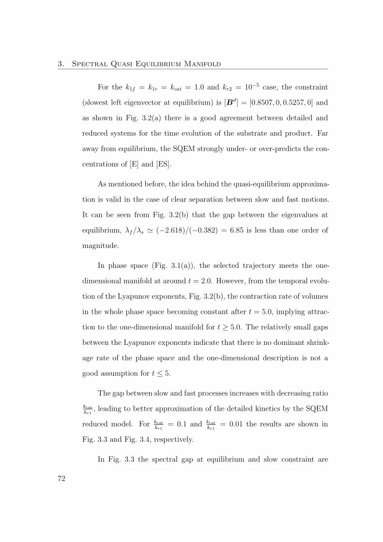
3. Spectral Quasi Equilibrium Manifold
For the k1f = k1r = kcat = 1.0 and kr2 = 10−5 case, the constraint
(slowest left eigenvector at equilibrium) is [Bd] = [0.8507, 0, 0.5257, 0] and
as shown in Fig. 3.2(a) there is a good agreement between detailed and
reduced systems for the time evolution of the substrate and product. Far
away from equilibrium, the SQEM strongly under- or over-predicts the con-
centrations of [E] and [ES].
As mentioned before, the idea behind the quasi-equilibrium approxima-
tion is valid in the case of clear separation between slow and fast motions.
It can be seen from Fig. 3.2(b) that the gap between the eigenvalues at
equilibrium, λf/λs ' (−2.618)/(−0.382) = 6.85 is less than one order of
magnitude.
In phase space (Fig. 3.1(a)), the selected trajectory meets the one-
dimensional manifold at around t = 2.0. However, from the temporal evolu-
tion of the Lyapunov exponents, Fig. 3.2(b), the contraction rate of volumes
in the whole phase space becoming constant after t = 5.0, implying attrac-
tion to the one-dimensional manifold for t ≥ 5.0. The relatively small gaps
between the Lyapunov exponents indicate that there is no dominant shrink-
age rate of the phase space and the one-dimensional description is not a
good assumption for t ≤ 5.
The gap between slow and fast processes increases with decreasing ratio
kcatkr1
, leading to better approximation of the detailed kinetics by the SQEM
reduced model. For kcatkr1
= 0.1 and kcatkr1
= 0.01 the results are shown in
Fig. 3.3 and Fig. 3.4, respectively.
In Fig. 3.3 the spectral gap at equilibrium and slow constraint are
72
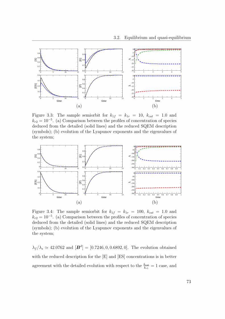
3.2. Equilibrium and quasi-equilibrium
0 5 10 150
0.2
0.4
0.6
0.8
1
[S]
0 5 10 150.6
0.7
0.8
0.9
1
[E]
0 5 10 15
time
0
0.1
0.2
0.3
0.4
[ES]
0 5 10 15
time
0
0.2
0.4
0.6
0.8
1
[P]
0 1 2 3 4 5-30
-25
-20
-15
-10
-5
0
Λ
0 1 2 3 4 5
time
-30
-25
-20
-15
-10
-5
0
λ
(a) (b)
Figure 3.3: The sample semiorbit for k1f = k1r = 10, kcat = 1.0 andkr2 = 10−5. (a) Comparison between the profiles of concentration of speciesdeduced from the detailed (solid lines) and the reduced SQEM description(symbols); (b) evolution of the Lyapunov exponents and the eigenvalues ofthe system;
0 5 10 150
0.2
0.4
0.6
0.8
[S]
0 5 10 150.6
0.7
0.8
0.9
1
[E]
0 5 10 15
time
0
0.1
0.2
0.3
0.4
[ES]
0 5 10 15
time
0
0.2
0.4
0.6
0.8
1
[P]
0 0.1 0.2 0.3 0.4 0.5 0.6 0.7 0.8 0.9 1-300
-250
-200
-150
-100
-50
0
Λ
0 0.1 0.2 0.3 0.4 0.5 0.6 0.7 0.8 0.9 1
time
-300
-250
-200
-150
-100
-50
0
λ
(a) (b)
Figure 3.4: The sample semiorbit for k1f = k1r = 100, kcat = 1.0 andkr2 = 10−5. (a) Comparison between the profiles of concentration of speciesdeduced from the detailed (solid lines) and the reduced SQEM description(symbols); (b) evolution of the Lyapunov exponents and the eigenvalues ofthe system;
λf/λs ' 42.0762 and [Bd] = [0.7246, 0, 0.6892, 0]. The evolution obtained
with the reduced description for the [E] and [ES] concentrations is in better
agreement with the detailed evolution with respect to the kcatkr1
= 1 case, and
73

3. Spectral Quasi Equilibrium Manifold
the SQEM trajectory approaches the detailed one much earlier. For kcatkr1
=
0.01 (Fig. 3.4), the agreement between the detailed and reduced model
for all species is excellent. The constraint is [Bd] = [0.7089, 0, 0.7053, 0]
and the spectral gap at equilibrium is more than two orders of magnitude,
λf/λs ' 401.96, implying the clear separation of timescales.
3.3 Results: Autoignition of homogeneous mix-
tures
In the following section the application of SQEM reduced model is demon-
strated for the detailed combustion mechanisms of hydrogen, syngas and
methane corresponding to 6-, 8- and 27-dimensional systems. Thermody-
namic properties and reaction rates were evaluated using CHEMKIN [104]
and the convex minimization problem (2.22) is solved using the CEQ code
[81].
3.3.1 H2/air mixture
The detailed kinetics scheme of hydrogen/air mixture includes ns = 9
species and nr = 21 reactions [17]. In the scope of RCCE applications
for hydrogen combustion, the total number of moles (TM), the total num-
ber of radicals referred to active valence (AV), and free oxygen (FO) are
linear constraints proposed in [67, 70] as an appropriate set of constraints
in the scope of RCCE applications for hydrogen combustion (Table 2.1).
The evolution of temperature for a stoichiometric hydrogen/air mixture
74

3.3. Results: Autoignition of homogeneous mixtures
at atmospheric pressure with initial temperature T0 = 1200 K is plotted in
Fig. 3.5. The detailed (solid line) solution is compared with SQEM (lines
with symbols) and RCCE manifold (dashed, dotted and dot-dashed lines).
It can be seen that with increasing dimension (number of constraints) the
agreement between the reduced and detailed description improves, and that
for the same dimension the SQEM provides a more accurate description.
0.0 5.0×10⁻⁵
1.0×10⁻⁴
1.5×10⁻⁴
2.0×10⁻⁴
2.5×10⁻⁴
t [s]
1000
1200
1400
1600
1800
2000
2200
2400
2600
2800
3000
T [
K]
Detailed
RCCE 1 Const.
RCCE 2 Const.
RCCE 3 Const.
SQEM 1 Const.
SQEM 2 Const.
SQEM 3 Const.
Figure 3.5: The temperature evolution for stoichiometric H2/air auto-ignition under atmospheric pressure with unburnt temperature T0 =1200K. Detailed solution is compared with RCCE and SQEM reduced modelswith different number of constraints.
For finding a better approximation of the ignition delay time, the ini-
tial composition of the constrained equilibrium state should approximate
the actual initial composition [70]. Fig. 3.5 shows that the initial state is
75

3. Spectral Quasi Equilibrium Manifold
not located near the one-dimensional quasi-equilibrium manifold which is
constructed based on one constraint in RCCE (1 Const., TM) and SQEM
(slowest left eigenvector at equilibrium).
The temporal evolution of species mass fractions using the three-dim-
ensional reduced QEM models are plotted in Fig. 3.6. SQEM provides a
more accurate description even for the low concentration species (hydroper-
oxy radical HO2 and hydrogen peroxide H2O2).
0.0 5.0×10⁻⁵
1.0×10⁻⁴
1.5×10⁻⁴
2.0×10⁻⁴
2.5×10⁻⁴
0
0.001
0.002
0.003
0.004
0.005
0.006
YH
DetailedRCCE 3 Const.SQEM 3 Const.
0.0 5.0×10⁻⁵
1.0×10⁻⁴
1.5×10⁻⁴
2.0×10⁻⁴
2.5×10⁻⁴
0
0.005
0.01
0.015
0.02
0.025
0.03
YO
H
0.0 5.0×10⁻⁵
1.0×10⁻⁴
1.5×10⁻⁴
2.0×10⁻⁴
2.5×10⁻⁴
t [s]
0.0
2.5×10⁻⁵
5.0×10⁻⁵
7.5×10⁻⁵
1.0×10⁻⁴
YH
O2
0.0 5.0×10⁻⁵
1.0×10⁻⁴
1.5×10⁻⁴
2.0×10⁻⁴
2.5×10⁻⁴
t [s]
1×10⁻⁶
1×10⁻⁵
1×10⁻⁴
YH
2O
2
Figure 3.6: Time history of selected species mass fractions for stoichiometricH2/air auto-ignition under atmospheric pressure with unburnt temperatureT0 =1200 K. Detailed solution is compared with three-dimensional RCCEand SQEM reduced models.
3.3.2 Syngas/air mixture
The CO/H2/O2 elementary scheme of Li et al. [17] was used for the chem-
istry description with 32 non-duplicate elementary reversible reactions and
76

3.3. Results: Autoignition of homogeneous mixtures
12 chemical species. For a stoichiometric mixture of syngas/air in an adia-
batic constant pressure reactor with T0 = 1200 K, the temperature evolution
captured from the detailed kinetics is compared with those found by SQEM
reduced descriptions of different dimension. It is shown that for two CO:H2
molar ratios rCO/H2 = 1/3 and 3 (Fig. 3.7 (a) and (b)) the agreement of the
SQEM with three constraints and the detailed mechanism for the ignition
delay time and the temperature time history is excellent.
0 1×10⁻⁴
2×10⁻⁴
3×10⁻⁴
4×10⁻⁴
t [s]
1000
1200
1400
1600
1800
2000
2200
2400
2600
2800
3000
T [
K]
Detailed
SQEM 1 Const.
SQEM 2 Const.
SQEM 3 Const.
0 2×10⁻⁴
4×10⁻⁴
6×10⁻⁴
8×10⁻⁴
1×10⁻³
t [s]
1000
1200
1400
1600
1800
2000
2200
2400
2600
2800
3000
T [
K]
Detailed
SQEM 1 Const.
SQEM 2 Const.
SQEM 3 Const.
(a) (b)
Figure 3.7: The temperature evolution for stoichiometric syngas/air auto-ignition under atmospheric pressure with unburnt temperature T0 =1200 K.Detailed solution is compared with SQEM reduced models with differentconstraints for (a) rCO/H2 = 1/3 and (b) rCO/H2 = 3.
3.3.3 Methane/air mixture
The GRI 1.2 mechanism [105] is used to predict the oxidation rates of CH4.
The detailed mechanism includes 31 species and 175 elementary reactions
with four elemental conservations (H, O, C and N); hence, the system is
27-dimensional. The temperature evolution for the stoichiometric mixture
77

3. Spectral Quasi Equilibrium Manifold
with T0 = 1400 K, p = 1 atm is plotted in Fig. 3.8 shows that SQEM with
seven constraints can capture the temperature behavior perfectly mean-
ing that the 27-dimensional system in this case can be represented with
7-dimensional reduced order model.
0 2×10⁻³
4×10⁻³
6×10⁻³
8×10⁻³
1×10⁻²
t [s]
1000
1200
1400
1600
1800
2000
2200
2400
2600
2800
T [
K]
Detailed
SQEM 4 Const.
SQEM 5 Const.
SQEM 6 Const.
SQEM 7 Const.
Figure 3.8: The temperature evolution for stoichiometric methane/air auto-ignition under atmospheric pressure with unburnt temperature T0 =1400 K.Detailed solution is compared with SQEM reduced models with differentconstraints.
It should be pointed out that the discrepancy between the reduced
and the detailed descriptions reduces non-monotonically with the dimension
of the SQEM model. Similar observations were made in other classes of
chemical kinetics model reduction methods based on species elimination
techniques [106,107].
78

3.4. Conclusion
Profiles of selected species found by SQEM six- and seven-dimensional
reduced manifolds are compared with the detailed model in Fig. 3.9, ex-
hibiting good agreements for the reduced model with seven constraints.
0 0.001 0.002 0.003 0.004 0.005 0.006
0
1×10⁻⁵
2×10⁻⁵
3×10⁻⁵
4×10⁻⁵
YC
2H
5
Detailed
SQEM 6 Const.
SQEM 7 Const.
0 0.001 0.002 0.003 0.004 0.005 0.006
0
0.02
0.04
0.06
0.08
YC
O
0 0.001 0.002 0.003 0.004 0.005 0.006
t [s]
0
0.0025
0.005
0.0075
0.01
0.0125
YC
2H
4
0 0.001 0.002 0.003 0.004 0.005 0.006
t [s]
0
0.002
0.004
0.006
0.008
YC
H3
Figure 3.9: Time history of selected species mass fractions for stoichiometricmethane/air auto-ignition under atmospheric pressure with unburnt tem-perature T0 =1400 K. Detailed solution is compared with SQEM reducedmodels with different constraints.
3.4 Conclusion
The spectral quasi-equilibrium manifolds based on the slow left eigenvectors
at equilibrium can be used to obtain accurate reduced descriptions for com-
bustion kinetics. The construction of the quasi-equilibrium states is based
on the concave optimization of an entropy function under the constraints
defined by the left eigenvectors on the number of moles of species. These
states belong to the Spectral Quasi Equilibrium Manifold (SQEM), which
shows better approximation of reduced model in comparison to RCCE-
79

3. Spectral Quasi Equilibrium Manifold
manifold routinely used in the combustion community. SQEM offers a gen-
eral mathematically-based procedure to define the constraints imposed on
the species and it is automated for any comprehensive/skeletal mechanisms.
The autoignition of hydrogen, syngas and methane shows very good agree-
ment between the time history of the temperature and radicals deduced
from reduced and detailed models.
Although the results of SQEM is promising by itself, it can be used
for construction of slow invariant manifolds in the class of approaches in
which an initial grid is iteratively relaxed towards SIM, such as Method of
Invariant Grid [92,93] and the algorithm proposed in Ref. [16].
80

Chapter 4
Entropy production analysis for
mechanism reduction 1
4.1 Introduction
In this chapter we will present the method developed during our study
categorized under skeletal reduction techniques.
Briefly, skeletal mechanisms can be generated by eliminating reactions
and/or species [108,109]. Elimination of unimportant reactions can be per-
formed using, for example, sensitivity analysis [21], the importance index of
CSP [110], Principal Component Analysis (PCA) [22] or optimization-based
methods [12,111]. Due to their nonlinear coupling, the direct elimination of
species is more challenging. CSP [33,110,112–114], Directed Relation Graph
(DRG) [27, 115–118], DRG with Error Propagation (DRGEP) [119, 120],
DRG-Aided Sensitivity Analysis (DRGASA) [121, 122], Transport Flux-
1The content of the present chapter is published in Kooshkbaghi, M., Frouzakis, C.E., Boulouchos, K., & Karlin, I. V. (2014). Entropy production analysis for mechanismreduction. Combustion and Flame, 161(6), 1507-1515.
81

4. Entropy production analysis for mechanism reduction
Based DRG (TFBDRG) [123], Path Flux Analysis (PFA) [24,28] and neces-
sity analysis [30] have been employed for species elimination. Species with
similar thermal and transport properties and diffusivities can be lumped
together to further reduce the size of the skeletal mechanism [124–126]. Se-
lecting important species during the simulation (on the fly model reduction)
is also possible as proposed for example by the Dynamic Adaptive Chem-
istry (DAC) reduction method [127,128]. The aforementioned methods can
be combined with storage/retrieval approaches [129]. A more comprehen-
sive discussion is available in chapter 1 and the references therein.
For large mechanisms, approaches which select species based on the sl-
ow/fast decomposition bear heavy computational cost because of the times-
cale analysis of the Jacobian matrix of the associated large system of ODEs.
On the other hand, QSSA, PEA and sensitivity analysis require additionally
mechanism-dependent knowledge. The methods which are based on the
graph structure relation between species, sometimes need a careful a priori
choice of the group of target species [127].
In the present study, the relative contribution of elementary reactions
in the total entropy production is proposed as a criterion for the construc-
tion of accurate skeletal reaction mechanisms. The important reactions are
identified based on their relative contribution to the total entropy produc-
tion being larger than a user-specified threshold. Entropy production is the
well known scalar function for reactive systems with some natural properties
such as positivity. This criterion leads to a procedure that is easy to imple-
ment without any prior knowledge about the detailed mechanism. Skeletal
82

4.1. Introduction
mechanisms of different sizes can be obtained by choosing the threshold
based on the desired deviation from the result of the detailed mechanism.
A significant reduction in the number of species as well as the stiff-
ness of the system is reported here for the case of a detailed scheme for
n-heptane. The skeletal mechanisms are shown to provide very accurate
results at a fraction of the computational cost in comparison to the detailed
mechanism for various cases over a wide range of thermodynamic conditions.
Compared to the other methods such as Directed Relation Graph (DRG)
and Computational Singular Perturbation (CSP) [114, 116], the same level
of reduction can be achieved with the much simpler entropy production
analysis.
The chapter is organized as follows. In Sec. 4.2, the basic notion of the
entropy production for chemical kinetics is briefly reviewed. The features
and algorithm of the method for skeletal mechanism reduction are presented
in Sec. 4.3. In Sec. 4.4, the algorithm is applied on a database generated
using a detailed n-heptane mechanism and two skeletal mechanisms are
compared. In the remaining part of Sec. 4.4 the ignition delay calculation,
homogeneous engine model, perfectly stirred reactor and laminar premixed
flame are used for the validation of the skeletal mechanism. Conclusions are
drawn in Sec. 4.5. Instructions on the numerical procedure of the entropy
production analysis are presented in the appendix A.
83

4. Entropy production analysis for mechanism reduction
4.2 Entropy production for chemical kinetics
For the sake of completeness, the notion of the entropy production is briefly
reviewed in this section following the formalism of [130]. For a detailed
discussion of the entropy and entropy production concepts for chemical
kinetics and other systems the reader is also referred to [59,71]. The changes
in the entropy for a system at local equilibrium is expressed as
dS = dexS + dinS (4.1)
where superscripts ‘in’ and ‘ex’ denote the change of the system entropy
due to interactions inside the domain and with its environment [130]. The
change of the i-th species in the k-th reaction is related to the change in
the extent of each reaction, ζk, as
dNi
ν ′′ik − ν ′ik= dζk, i = 1, · · · , ns k = 1, · · · , nr (4.2)
where the extent of reaction is related to the reaction rate by
dζkdt
= V (qfk − qrk) (4.3)
The fundamental equation of chemical thermodynamics in terms of the
internal energy reads
dU = TdS − pdV +ns∑i=1
µidNi (4.4)
84

4.2. Entropy production for chemical kinetics
where µi is the chemical potential of the i-th species
µi =
(∂U
∂Ni
)S,V,Nl 6=i
, i = 1, · · · , ns (4.5)
The de Donder affinity [131] of reaction k is defined as
αk = −Σnsi=1(ν ′′ik − ν ′ik)µi, k = 1, · · · , nr (4.6)
In the absence of deviations from the principle of detailed balance [71], αk
may be expressed as
αk = RcT ln
(qfkqrk
)(4.7)
The change in the number of moles of each species can be decomposed into
the change due to chemical reactions, dinNi, and exchange of matter with
the system exterior, dexNi [132].
dNi = dinNi + dexNi, i = 1, · · · , ns (4.8)
For open systems, the entropy exchange with the exterior is of the form
dexS =dU + pdV
T−∑ns
i=1 µidexNi
T(4.9)
while the entropy change due to the change in mole numbers with respect
to chemical reactions reads
dinS = −∑ns
i=1 µidinNi
T(4.10)
85

4. Entropy production analysis for mechanism reduction
For a closed system, dexN = 0 so that dN = dinN and the entropy
production due to a chemical reaction is,
dinS
dt= − 1
T
ns∑i=1
µidNi
dt(4.11)
where dNidt
can be written in terms of the extent of reactions using (4.2)
dNi
dt=
nr∑k=1
(ν ′′ik − ν ′ik)dζkdt
(4.12)
Hence, entropy production is
dinS
dt= − 1
T
ns∑i=1
µi
nr∑k=1
dζkdt
(ν ′′ik − ν ′ik) (4.13)
or by the affinity definition (4.6),
dinS
dt=
1
T
nr∑k=1
αkdζkdt
(4.14)
Using (4.3) and (4.7), the total entropy production per unit volume becomes
dinS
dt= Rc
nr∑k=1
(qfk − qrk) ln
(qfkqrk
)≥ 0 (4.15)
The entropy production (4.15) is a positive semi-definite function which
vanishes at equilibrium. The relative contribution of each reaction to the
total entropy production at time t, rk(t) is finally defined as
rk(t) =
(dinS
dt
)−1 [Rc(qfk − qrk) ln
(qfkqrk
)](4.16)
86

4.3. Skeletal reduction using entropy production analysis
From equation (4.16) it is clear that for the reactions at equilibrium rk(t) =
0.
4.3 Skeletal reduction using entropy production
analysis
In this chapter, the relative contribution of each reaction to the total entropy
production is considered as a measure of its importance. The steps for
finding the subset of the reactions that at the time t of interest forms the
skeletal mechanism are summarized below:
1. Identify the most-contributing reactions, i.e. the reactions which con-
tribute at least ε to the total entropy production
rk(t) ≥ ε (4.17)
2. Identify the important species, i.e. the species participating in the
most-contributing reactions.
3. Generate the skeletal mechanism. The simplified mechanism at time
t is generated by eliminating the non-important species from the de-
tailed description using a slightly modified version of MECHMOD
3.42 [133].
Note that each important species participate in at least one most-con-
tributing reaction. Following step 3, the skeletal mechanism contains not
only the most contributing reactions, but all elementary reactions which
87

4. Entropy production analysis for mechanism reduction
include important species on both sides as well. Further reduction of the
number of reactions (with the same amount of species) would necessities
further analysis such as reaction path or atomic flux [24] to quantify the
contribution of each reaction in the total production or consumption rate
of each species.
The local analysis of the entropy production can be applied at differ-
ent time instants during the temporal evolution of the system state. The
analysis can be extended to a database of trajectories computed for a range
of pressures, initial temperatures and compositions to construct a global
skeletal mechanism. The most-contributing reactions are considered as the
reactions which at least once have a significant contribution in the entropy
production of the whole database. The final skeletal mechanism is valid
within the range of conditions represented by the sample data. The algo-
rithm of the present simple procedure is provided in the appendix A using
CHEMKIN’s notation.
Finally, it should be pointed out that the term qfk/qrk in the logarithm
of (4.15) must be strictly positive. This condition is violated in two cases:
(a) irreversible reactions where the backward reaction rate is zero (qrk = 0);
(b) when low negative concentrations result from numerical issues (qfk < 0
and/or qrk < 0).
In case (a) the qrk , and in the case (b) qfk and/or qrk should be set to be
a small (chemically insignificant) positive number (e.g. 10−50 in our study).
The problem of partially irreversible limit in chemical thermodynamics is
88

4.4. Skeletal mechanism for n-heptane
addressed in the recent study [134].
4.4 Skeletal mechanism for n-heptane
The kinetics of n-heptane is of interest not only in its own right as rep-
resentative of the kinetics of higher hydrocarbons displaying the Negative
Temperature Coefficient (NTC) regime and multistage ignition, but also as
one of the components of the Primary Reference Fuel (PRF) used for octane
rating of internal combustion engines [135]. The comprehensive mechanism
for n-heptane consisting of 561 species and 2539 reactions (LLNL mech-
anism version 2, [136]) was developed to study oxidation for pressures in
the range 1 ≤ p ≤ 42 atm, initial temperatures between 550 to 1700 K,
equivalence ratio ϕ from 0.3 to 1.5, and nitrogen-argon dilution from 70 to
99 percent [4]. The detailed mechanism which will be referred to as D561
below has been used for the development of reduced schemes by various
approaches [114,116,117,126,137].
The local entropy production analysis is performed at the four time
instants during the isobaric and isenthalpic auto-ignition of a stoichiometric
mixture at initial temperature and pressure T0 = 650 K, p = 1 atm marked
in Fig. 4.1 to identify the reactions contributing at least ε = 0.05 to the
total entropy production. The analysis reveals that initially (t = 0 s) the
important reactions are the initiation reaction of oxygen attacking the fuel
89
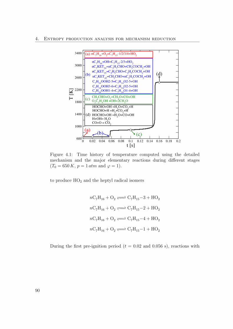
4. Entropy production analysis for mechanism reduction
0 0.02 0.04 0.06 0.08 0.1 0.12 0.14 0.16 0.18 0.2
t [s]
600
1000
1400
1800
2200
2600
3000
3400
T [
K]
(a)(b) (c)
CH2CHO+O
2=CH
2O+CO+OH
nC7H
16+O
2=C
7H
15-1/2/3/4+HO
2
C7H
14OOH1-4=C
7H
14O1-4+OH
(d)
nC7KET
24=nC
3H
7CHO+CH
3COCH
2+OH
nC7KET
35=C
2H
5CHO+C
2H
5COCH
2+OH
nC7KET
42=CH
3CHO+nC
3H
7COCH
2+OH
O2C
2H
4OH =OH+2CH
2O
(d)HOCHO+H =H
2+CO
2+H
HOCHO+OH =H2O+CO
2+H
HOCHO+OH =H2O+CO+OH
(a)
(b)
(c)
nC7H
16+OH=C
7H
15-2/3+HO
2
C7H
14OOH2-5=C
7H
14O2-5+OH
C7H
14OOH3-6=C
7H
14O2-5+OH
CO+O = CO2
H+OH= H2O
Figure 4.1: Time history of temperature computed using the detailedmechanism and the major elementary reactions during different stages(T0 = 650K, p = 1 atm and ϕ = 1).
to produce HO2 and the heptyl radical isomers
nC7H16 + O2−−−− C7H15−3 + HO2
nC7H16 + O2−−−− C7H15−2 + HO2
nC7H16 + O2−−−− C7H15−4 + HO2
nC7H16 + O2−−−− C7H15−1 + HO2
During the first pre-ignition period (t = 0.02 and 0.056 s), reactions with
90

4.4. Skeletal mechanism for n-heptane
OH radicals abstracting H from the fuel
nC7H16 + OH −−−− C7H15−2 + H2O
nC7H16 + OH −−−− C7H15−3 + H2O
thermal decomposition
C7H14OOH2−5 −−−− C7H14O2−5 + OH
C7H14OOH3−6 −−−− C7H14O2−5 + OH
C7H14OOH1−4 −−−− C7H14O1−4 + OH
and ketohydroperoxides decomposition
nC7ket24 −−→ nC3H7CHO + CH3COCH2 + OH
nC7ket35 −−→ C2H5CHO + C2H5COCH2 + OH
contribute significantly to the entropy production. The most-contributing
reactions during the period before the second ignition (t = 0.1 s) are the
ones producing formaldehyde (CH2O) and carbon monoxide (CO)
CH2CHO + O2 −−→ CH2O + CO + OH
O2C2H4OH −−→ OH + 2 CH2O
The analysis of post-ignition at t = 0.16 s shows that the most-contributing
91

4. Entropy production analysis for mechanism reduction
reactions are those producing the main products (CO2, CO and H2O)
HOCHO + OH −−→ H2O + CO2 + H
HOCHO + H −−→ H2 + CO2 + H
HOCHO + OH −−→ H2O + CO + OH
The distribution of entropy production among reactions for different times
are summarized in Fig. 4.2. It is worth to pointing out that the important
0 10 20 30 40
nC7H16 + O2 = C7H15−1 +HO2
nC7H16 + O2 = C7H15−4 +HO2
nC7H16 + O2 = C7H15−2 +HO2
nC7H16 + O2 = C7H15−3 +HO2
%rk
0 2 4 6 8 10 12 14
C7H14OOH3−5O2 = nC7ket35 + OH
C7H14OOH2−4O2 = nC7ket24 + OH
nC7H16 + OH = C7H15−3 +H2O
nC7H16 + OH = C7H15−2 +H2O
nC7ket42 = CH3CHO + nC3H7COCH2 + OH
nC7ket35 = C2H5CHO + C2H5COCH2 + OH
nC7ket24 = nC3H7CHO + CH3COCH2 + OH
C7H14OOH1−4 = C7H14O1−4 + OH
C7H14OOH3−6 = C7H14O2−5 + OH
C7H14OOH2−5 = C7H14O2−5 + OH
rk × 102
(a) (b)
0 2 4 6 8 10 12
C2H3 + O2 = CH2O +HCO
C4H8OH−1O2 = C2H5CHO + CH2O + OH
2OH(+M) = H2O2(+M)
HOCHO +HO2 = H2O2 + CO + OH
C7H14O2−5 + OH = CH3COCH2 + C4H8−1 +H2O
C7H14O2−5 + OH = C3H6 + C2H5COCH2 +H2O
CH2O + OH = HCO +H2O
HCO + O2 = CO +HO2
O2C2H4OH = OH + 2CH2O
CH2CHO + O2 = CH2O + CO + OC
%rk
0 10 20 30 40 50 60 70
HOCHO +H = H2 + CO + OH
HOCHO + OH = H2O + CO + OH
HOCHO +H = H2 + CO2 +H
HOCHO + OH = H2O + CO2 +H
%rk
(c) (d)
Figure 4.2: Entropy production distributions among reactions using thedetailed mechanism (T0 = 650K, p = 1 atm and ϕ = 1); (a) t = 0 s, (b)t = 0.03 s, (c) t = 0.1 s, (d) t = 0.16 s.
reactions, products and oxidation path found here on the basis of the en-
tropy production analysis are in agreement with the results of the kinetic
description of n-heptane oxidation [4] and the CSP analysis [114].
92

4.4. Skeletal mechanism for n-heptane
Entropy production analysis was then performed on a solution database
for auto-ignition in the range of pressures 1, 5, 10, 20 atm, initial temper-
atures in the range 650 ≤ T0 ≤ 1400 K resolved with a step of 50 K,
equivalence ratios ϕ =0.5, 0.8, 1.0, 1.2, 1.5 and different threshold values ε.
The dependence of the error in the ignition delay time and the number of
species in the skeletal mechanism on the value of ε are plotted in Fig. 4.3
for p = 1 atm, T0 = 650 K and ϕ = 1.0. The non-monotonicity of the error
curve has also been observed in other species elimination techniques based
on analysis of reactive states [28,106].
0
50
100
150
200
250
300
350
400
450
500
550
600
Nu
mb
er o
f S
pec
ies
Number of Species
0 0.005 0.01 0.015 0.02
ε
0.001
0.01
0.1
1
10
100
Ign
itio
n d
elay
err
or
%
Ignition delay error
T0 = 650 K
p = 1atmφ = 1.0
Figure 4.3: Number of species in the skeletal mechanism and relative errorin the ignition delay time as a function of the threshold.
Two skeletal mechanisms with 161 species in 688 reactions and 203
species in 879 reactions obtained with ε = 0.006 and 0.002 and henceforth
93
4. Entropy production analysis for mechanism reduction
referred to as R161 and R203, respectively, were selected for validation. It
should be noted that smaller schemes can be readily constructed, albeit at
the cost of narrower range of applicability and/or lower accuracy. Similar
species can also be lumped together as proposed in [117, 126] to further
reduce the size of the mechanism.
The size of the mechanism obtained by the entropy production analysis
is comparable with other reducing strategies. With the same quality of
reduction, skeletal mechanisms including 188 species and 842 reactions was
obtained by DRG [116], and 177 species and 768 reactions or 185 species
and 786 reactions by CSP [114].
4.4.1 Auto-ignition of homogeneous mixtures
Ignition delay times in the constant pressure and enthalpy reactor computed
using the skeletal and detailed mechanisms are compared in Fig. 4.4. Both
skeletal mechanisms reproduce the ignition delay well over a wide range of
pressures, equivalence ratios and temperatures including the NTC region.
As expected, better agreement is obtained at high pressures and tempera-
tures and the error for R161 is higher than that of R203.
Species elimination with the help of entropy production leads not only
to an ODE system of reduced dimensionality but also with lower stiffness.
The evolution of the fastest timescale, τfast, defined by the inverse of the
most negative eigenvalue of the Jacobian matrix for the D561, R203 and
R161 schemes is plotted in Fig. 4.5, together with the time history of temper-
ature. The fast timescale is monotonically decreasing towards equilibrium,
94

4.4. Skeletal mechanism for n-heptane
0.8 1 1.2 1.4 1.6
1000/T0 [1/K]
10-5
10-4
10-3
10-2
10-1
100
τig
[s]
φ = 0.5
φ = 1.0
φ = 1.5
φ = 0.5
φ = 1.0
φ = 1.5
p = 1 atm
p = 20 atm
Figure 4.4: Ignition delay times computed with the different mechanisms(D561: solid line, R203: circles, R161: dashed line).
while there are sharp drops during the two ignition stages. The difference
between the timescales of the detailed and skeletal mechanisms are sev-
eral orders of magnitude which in combination with the reduced number of
variables results in a significant reduction in computational time even for
homogeneous autoignition computations. CPU times for the calculation of
1 s of the ignition process for three initial temperature are summarized in
Table 4.1 using the stiff integrator DVODE [84]. The CPU calculation times
reveals that the speed up for R203 and R161 compared with D561 is around
10.3 and 16, respectively. Similar order of timescales for n-heptane was also
reported in [137]. It should be noted that the unrealistically fast time scales
of the order of 10−15 s may well be an artifact of the way the detailed mech-
95
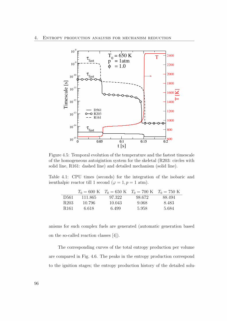
4. Entropy production analysis for mechanism reduction
0 0.05 0.1 0.15 0.2
t [s]
600
800
1000
1200
1400
1600
1800
2000
2200
2400
T [
K]
0 0.05 0.1 0.15 0.210
-15
10-14
10-13
10-12
10-11
10-10
10-9
10-8
Tim
esca
le [
s]
D561R203R161
T τfast
τfast
τfast
T0 = 650 K
p = 1atmφ = 1.0
Figure 4.5: Temporal evolution of the temperature and the fastest timescaleof the homogeneous autoigintion system for the skeletal (R203: circles withsolid line, R161: dashed line) and detailed mechanism (solid line).
Table 4.1: CPU times (seconds) for the integration of the isobaric andisenthalpic reactor till 1 second (ϕ = 1, p = 1 atm).
T0 = 600 K T0 = 650 K T0 = 700 K T0 = 750 KD561 111.865 97.322 98.672 88.494R203 10.796 10.043 9.068 8.483R161 6.618 6.499 5.958 5.684
anisms for such complex fuels are generated (automatic generation based
on the so-called reaction classes [4]).
The corresponding curves of the total entropy production per volume
are compared in Fig. 4.6. The peaks in the entropy production correspond
to the ignition stages; the entropy production history of the detailed solu-
96

4.4. Skeletal mechanism for n-heptane
tion is well reproduced by both R203 and R161. At equilibrium the entropy
reaches its maximum and dS/dt tends to zero (Fig. 4.6) albeit at a decreas-
ing rate (Eq. 4.15). In the presence of irreversible reactions and negative
0 0.05 0.1 0.15
t [s]
10-12
10-10
10-8
10-6
10-4
10-2
100
dS
/dt
[J/
K s
cm
3]
D561R203R161
600
1000
1400
1800
2200
2600
3000
3400
3800
4200
T [
K]
T0 = 650 K
p = 1 atmφ = 1.0
Figure 4.6: Time history of the entropy production (D561: solid line, R203:circles, R161: dashed line).
concentration resulting from numerical issues (as is the case here), the value
of dS/dt at long times is affected by the value chosen for the regularization
of zero (or negative) reaction rates (see section 4.3).
4.4.2 Single-zone engine model
In the absence of spatial inhomogeneities, a single-zone model can be used to
simulate a reciprocating engine with adiabatic boundary conditions [138].
The governing equations for the temporal evolution of the species mass
97

4. Entropy production analysis for mechanism reduction
Figure 4.7: Schematic picture of single-zone engine model with dimensions.
fractions, Yi, temperature and pressure read
dYidt
=ωiWi
ρ
dT
dt=
1
cv
(−pd(1/ρ)
dt−∑
i eiωiWi)
ρ
)(4.18)
p =RcTρ
W
where, ρ, W and cv are the density, mean molecular weight and mean spe-
cific heat at constant volume of the mixture, and Rc the ideal gas constant.
Thermodynamic properties, production rates, ωi, and specific internal en-
ergy, ei, of the ith species are computed, using the CHEMKIN library [104].
The change of density in time is the function of the cylinder volume and
the total mass of the reacting mixture. The change of volume, V (t), can be
98

4.4. Skeletal mechanism for n-heptane
related to the crank angle, θ [138]
V (t)
Vc= 1 +
1
2(rc − 1)f(θ) (4.19)
with
f(θ) = l/a+ 1− cos(θ(t))−√
(l/a)2 − sin(θ(t)) (4.20)
where, Vc is the clearance volume (minimum cylinder volume), l/a is the
Crank Angle [0ATDC]
T[K
]
40 20 0 20 40 60 80 100
1000
1500
2000
2500
Crank Angle [0ATDC]
p[atm
]
40 20 0 20 40 60 80 100
10
20
30
40
(a) (b)
Crank Angle [0ATDC]
MassFraction
40 20 0 20 40 60 80 10010
5
104
103
102
101
CO2
H2O
COnC
7H
16
Crank Angle [0ATDC]
MassFraction
40 20 0 20 40 60 80 100
1010
108
106
104
102
OH
HO2
H2O
2
CH2O
HCO
(c) (d)
Figure 4.8: Temperature (a), pressure (b) and selected species concentration(c,d) profiles for the single-zone engine model. The lean fresh mixture (ϕ =0.8) is injected at −40 0ATDC with p0 = 5 atm and T0 = 750 K (D561:solid line, R203: circles, R161: dashed line).
99

4. Entropy production analysis for mechanism reduction
ratio of the connecting rod length to the crank radius and rc is the compres-
sion ratio (see Fig. 4.7). The simulation are carried out for an engine with
Vc = 125 ml, l/a = 3 and rc = 10. The initial temperature and pressure for
the lean mixture (ϕ = 0.8) at −40 oATDC (after top dead center) are 750 K
and 5 atm, respectively. The pressure and temperature traces for 700 rpm
are compared in Fig. 4.8(a) and (b): the differences between the results are
of the same order as for the ignition delay. The profiles for selected species
in Fig. 4.8(c) and (d) show excellent agreement for the major species and
radicals even at very low concentrations. It should be noted that the skele-
tal mechanisms are constructed using data in the range 1 ≤ p ≤ 20 atm,
but in this case the pressure is increasing up to 47 atm. As mentioned in
section 4.4.1, the agreement between the skeletal and detailed models are
generally better at high pressures.
4.4.3 Premixed flame
The accuracy of the skeletal mechanisms generated using data for a homoge-
neous system were finally validated in an atmospheric 1-D laminar premixed
flame with an unburned mixture temperature Tu = 650 K using the PRE-
MIX code of CHEMKIN [87]. The laminar flame speed, SL, is reproduced
to within a maximum difference in the laminar flame speed for both R161
and R203 with respect to D561 that is less than 2 cm/s (Fig. 4.9(a)). The
computed flame temperatures Tf are in excellent agreement (Fig. 4.9(b)).
The flame structure is also accurately captured as shown in Fig. 4.10 for the
stoichiometric mixture. The computational time with the skeletal mecha-
100

4.4. Skeletal mechanism for n-heptane
0.7 0.8 0.9 1 1.1 1.2 1.3 1.4120
130
140
150
160
170
180
190
SL [
cm
/s]
0.7 0.8 0.9 1 1.1 1.2 1.3 1.4
φ
2200
2300
2400
2500
Tf [
K]
(a)
(b)
Figure 4.9: (a) Laminar flame speed SL and (b) flame temperature Tf (p = 1atm, unburned mixture temperature Tu = 650 K; D561: solid line, R203:circles, R161: dashed line).
nisms is at least one order of magnitude lower since the significant reduction
in the number of species drastically reduces the computational cost for the
evaluation of the right hand side and the Jacobian.
It should be stressed that Eq. (4.15) describes only the contribution of
the reaction to the total entropy production. However, the premixed flame
application demonstrates the validity of the skeletal mechanism generated
using homogeneous reactor results. In a laminar flame the total entropy
generation including not only chemical reactions but also, contribution of
viscosity, heat conduction and mass diffusion. It has been shown however
that the major process for entropy production is entropy generation due to
101

4. Entropy production analysis for mechanism reduction
X [cm]
Mass
Fraction
T[K
]
0 0.05 0.1 0.15 0.210
4
103
102
101
100
800
1200
1600
2000
2400
T
CO2
O2
nC7H
16
H2O
CO
X [cm]
Mass
Fraction
0 0.05 0.1 0.15 0.210
8
107
106
105
104
103
102
H
OH
O
H2
HO2
H2O
2
X [cm]
Mass
Fraction
0 0.05 0.1 0.15 0.210
8
107
106
105
104
103
HCO
CH4
CH
CH3
X [cm]
Mass
Fraction
0 0.05 0.1 0.15 0.210
8
107
106
105
104
103
102
C2H
6
C2H
5
C2H
4
Figure 4.10: Temperature and selected species profiles of the premixed lam-inar flame (p = 1 atm, Tu = 650 K and ϕ = 1; D561: solid line, R203:circles, R161: dashed line).
the chemical reactions [139].
4.5 Conclusions
In this work, we have proposed and validated the entropy production anal-
ysis for the skeletal reduction of detailed mechanisms. Important reactions
are identified based on their relative contribution to the total entropy pro-
duction above a user-specified threshold. Application to the detailed LLNL2
mechanism for n-heptane with 561 species resulted in skeletal mechanisms
102

4.5. Conclusions
with 203 and 161 species. The same comprehensive mechanism has been
used for skeletal reduction with different approaches. For 600 ≤ T ≤ 1800
K, 1 ≤ p ≤ 40 atm and 0.5 ≤ ϕ ≤ 1.5, 188 species by DRG, and for
700 ≤ T ≤ 1100 K, 6.5 ≤ p ≤ 40 atm and 0.5 ≤ ϕ ≤ 2.0, 177 and 185
species by CSP are available in the literature with comparable accuracy
with the skeletal mechanisms found by entropy production analysis. The
skeletal mechanisms exhibit good agreement not only for the homogeneous
auto-igniting system and a single-zone engine model, but also for the spa-
tially varying laminar premixed flames where diffusion plays an important
role. In addition to the lower number of species, the skeletal mechanisms are
less stiff than the detailed mechanism and computational implementations
show significant speedup.
The proposed approach can be easily applied on large detailed mecha-
nisms of realistic fuels to produce skeletal schemes with promising ratio of
reduction (e.g. 71% reduction for R161). The physical basis of the entropy
production analysis and the simplicity of the algorithm (see the appendix
A) warrants the investigation of its potential for the efficient adaptive (on-
the-fly) chemistry reduction.
103


Chapter 5
n-heptane/air complex dynamics
1
5.1 Introduction
The Perfectly Stirred Reactor (PSR) or Continuous Stirred Tank Reactor
(CSTR) is commonly used to study complex chemical kinetics and combus-
tion dynamics. In practice, such reactors can be realized by intense mixing
using gas reactant jets in a jet-stirred arrangement [140]. Efficient mixing
provides homogeneous conditions so that the reactor state at the exit is the
same as inside and strongly simplifies its numerical modeling.
Since the rigorous analysis of Bilous and Amundson in 1955 [141] and
the more comprehensive numerical study of Aris and Amundson [142], the re-
actor dynamics and stability for the single-step irreversible exothermic reac-
tion R→ P have been investigated extensively, revealing interesting dynam-
1The content of the present chapter is published in Kooshkbaghi, M., Frouzakis,C. E., Boulouchos, K., & Karlin, I. V. (2015). n-heptane/air combustion in perfectlystirred reactors: dynamics, bifurcations and dominant reactions at critical conditionsCombustion and Flame, 162(9), 3166-3179.
105

5. n-heptane/air complex dynamics
ics, including multiple equilibria and hysteresis loops, super- and subcritical
Hopf bifurcations, and complex oscillations (see, for example, [143–145]).
The dependence of the reactor state (indicated for example by the
reactor temperature T ) on τ , the residence time in the reactor, typically
displays an S-shaped curve, connecting the weakly- and strongly-burning
steady state branches via an unstable steady state branch between the ig-
nition and extinction points, which define the sudden transitions from one
stable state to another [146]. The lower branch of the bifurcation diagram
that shows the possible long-term states drawn schematically in Fig. 5.1
starts from the chemically frozen state at very short residence time and
remains weakly-reacting up to the residence time of ignition τign, where
the system state jumps to the strongly-burning branch. Starting from a
state on the latter branch, the gradual decrease of τ will eventually lead
the reactor back to the weakly-reacting state at τext, the residence time of
extinction. Steady state multiplicity exists for τext ≤ τ ≤ τign, and the
reactor operation becomes sensitive to external perturbations.
More complete pictures of the qualitative features of PSRs and phase
portraits for various scenarios of bifurcation diagram have been obtained
analytically and numerically for single-step reactions and lumped variables
[147–149]. PSRs have also been investigated via Lyapunov’s direct method
[150], parametric sensitivity [151] as well as from the control and stabiliza-
tion point of view (e.g. [152]). A discussion of earlier theoretical and exper-
imental studies of ignition and cool flames in CSTRs can be found in the
review of Griffiths and Scott [153], the book [145] and the references therein.
106

5.1. Introduction
Figure 5.1: Typical S-shaped bifurcation diagram of a PSR temperaturewith respect to the residence time.
The ignition and extinction conditions are used for the validation and rate
constant tuning of detailed and reduced mechanisms by comparison with
experimental data (see, for example, [8]).
Although the dynamic behavior of PSRs using generic single- or few-
steps reactions has been systematically analyzed in the literature, few stud-
ies have considered detailed reaction mechanisms. Numerical investigations
of hydrogen combustion in isothermal PSRs [154–156] revealed complex dy-
namics which in addition to ignitions and extinctions included oscillations
and birhythmicity (coexistence of two stable limit cycles for the same op-
erating conditions). Sensitivity and principal component analysis at the
bifurcation points were used to construct minimal reaction mechanisms
that can predict state multiplicity [155]. Recent investigations of igni-
tion/extinction behavior of more complex fuels like dimethyl ether [157,158]
and n-heptane [159] in PSRs focused on the detection of important features
with respect to the variation of a single parameter (the residence time) and
107

5. n-heptane/air complex dynamics
its effect on the type of extinction (sudden jump to the weakly-burning
or extinguished state or dynamic extinction via oscillations of increasing
amplitude) [158].
The complexity of the reaction mechanism in terms of the number
of species and reactions increases dramatically with the size of the fuel
molecule [160], and even for ideal homogeneous reactors like the PSR the
computational cost becomes high, particularly when a large number of pa-
rameters determines the behavior. Thanks to the availability of efficient
numerical continuation packages, the dynamic system analysis of single- or
few-steps global reactions can be expanded to detailed mechanisms includ-
ing hundreds of species and thousands of elementary reactions. The efficient
scanning of the dynamics with respect to multiple operating parameters can
identify the critical conditions leading to the transition between different
reactor states and provide essential information not only to enhance our
understanding of the phenomenology of combustion chemistry, but also for
the design of experiments for probing different types of kinetics and for
mechanism validation purposes.
In this chapter, we employ a skeletal mechanism of n-heptane con-
structed using the relative contribution of elementary reactions to the total
entropy production [107] presented in chapter 4.
The bifurcation diagram summarizing the possible dynamics as well as
the transitions leading from one state to another can be generated by find-
ing the long-time state for the system of equations describing the dynamics
for different values of the controlling parameter(s). In a brute force manner,
108

5.1. Introduction
this can be achieved by numerical integration of the transient equations
modeling the temporal evolution of the concentration and temperature in
the reactor (see Sec. 5.2) to scan the parameter space for different initial
conditions. However, this approach can only identify stable steady or oscil-
latory states.
The dynamics in a PSR is determined by five parameters: the residence
time τ , inlet temperature T0, pressure p, equivalence ratio ϕ and heat loss
per unit volume Qloss, and the brute force method becomes impractical.
Arc-length continuation methods [161] offer an accurate and more efficient
way to track changes in the long-term behavior by starting from a particular
solution and following it as one or more parameters are varied. The local sta-
bility can be determined by the eigenvalues of the Jacobian matrix obtained
from the linearization of the governing equations around the desired state:
eigenvalues with negative (positive) real parts define stable (unstable) states.
In this work the AUTO-07p package [162,163] is employed to systematically
follow the transitions in the observed behavior, first with respect to indepen-
dent variations of τ and Qloss for fixed values of the remaining parameters
(one-parameter continuations), and then for the simultaneous variation of
τ and T0 (two-parameter continuation). The effect of equivalence ratio and
pressure is assessed by computing the two-parameter diagrams for different
values of ϕ and p to partially construct three-parameter diagrams. The ob-
served dynamics include steady and oscillatory strongly-burning states and
cool flames, multistability over extended ranges of operating conditions and
higher co-dimension bifurcations.
109

5. n-heptane/air complex dynamics
As it was stated in chapter 4, entropy production analysis can also pro-
vide useful information about elementary reactions responsible for bringing
the system state to equilibrium. In this chapter it is complemented by in-
dices proposed in the context of the Computational Singular Perturbation
(CSP) method to analyze the kinetics at the bifurcation points. The CSP
analysis is performed on the mode with time scale corresponding to the
positive or the least negative eigenvalue of the Jacobian matrix at the state
of interest. The corresponding eigenvector, a first-order approximation to
the CSP mode, is used to identify the most important reactions at extinc-
tion, ignition or oscillatory combustion with the help of the amplitude [39]
and time scale participation [34] indices. More detailed CSP-based analy-
ses of autoignition and the multi-stage ignition of n-heptane can be found
in [164–166].
The work presented in this chapter is along the lines of the work of Lu
and co-workers who studied combustion dynamics in PSRs for n-heptane
[159], methane [157] and DME [157, 158]. One-parameter continuations
with respect to the residence time were performed in these works focusing
on ignition and extinction, and Chemical Explosive Mode Analysis (CEMA),
a variant of the CSP method [167], was employed to analyze the kinetics.
The chapter is organized as follows: Following the presentation of the
PSR governing equations in Sec. 5.2 and a brief discussion of numerical
continuation in Sec. 5.3, the skeletal mechanism that was generated using
entropy production analysis is presented in Sec. 5.4. The CSP analysis
tools used are briefly reviewed in Sec. 5.5 before turning to the results of
110
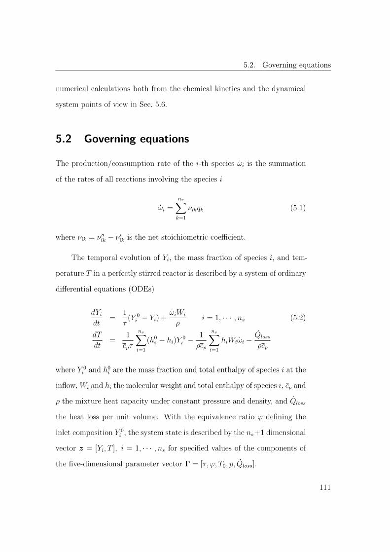
5.2. Governing equations
numerical calculations both from the chemical kinetics and the dynamical
system points of view in Sec. 5.6.
5.2 Governing equations
The production/consumption rate of the i-th species ωi is the summation
of the rates of all reactions involving the species i
ωi =nr∑k=1
νikqk (5.1)
where νik = ν ′′ik − ν ′ik is the net stoichiometric coefficient.
The temporal evolution of Yi, the mass fraction of species i, and tem-
perature T in a perfectly stirred reactor is described by a system of ordinary
differential equations (ODEs)
dYidt
=1
τ(Y 0
i − Yi) +ωiWi
ρi = 1, · · · , ns (5.2)
dT
dt=
1
cpτ
ns∑i=1
(h0i − hi)Y 0
i −1
ρcp
ns∑i=1
hiWiωi −Qloss
ρcp
where Y 0i and h0
i are the mass fraction and total enthalpy of species i at the
inflow, Wi and hi the molecular weight and total enthalpy of species i, cp and
ρ the mixture heat capacity under constant pressure and density, and Qloss
the heat loss per unit volume. With the equivalence ratio ϕ defining the
inlet composition Y 0i , the system state is described by the ns+1 dimensional
vector z = [Yi, T ], i = 1, · · · , ns for specified values of the components of
the five-dimensional parameter vector Γ = [τ, ϕ, T0, p, Qloss].
111

5. n-heptane/air complex dynamics
Starting from an initial condition z = z(t = 0), the initial value prob-
lem (5.2) can be integrated for specified values of the parameters using
the stiff ordinary differential equation solver DVODE [84] to compute the
temporal evolution of the reactor state. The chemical source term and the
thermodynamic properties are computed using CHEMKIN [104]. At long
times the system evolves towards either a steady (equilibrium) or an oscil-
latory state (limit cycle or periodic orbit). In general, bounded solutions
of systems of autonomous ODEs can also converge at long times to more
complex attractors, like tori (quasi-periodic orbits) or strange attractors
(chaotic orbits) (for example, see [168,169]).
5.3 Numerical bifurcation analysis
Time integration can be used to explore the dynamics in a brute-force way
for different combinations of parameters and initial conditions. In the gen-
eral case, slight changes of the parameters result in small changes of the
long-term dynamics, and the dynamical system displays structural stability.
However, at critical parameter values small variations can lead to bifurca-
tions where the change in the long-term dynamics can be dramatic. The
corresponding values or the zero-, one- or multi-dimensional loci of the crit-
ical parameters define the bifurcations points, curves, or surfaces which sep-
arate the parameter space into regions characterized by similar long-term
dynamics.
112
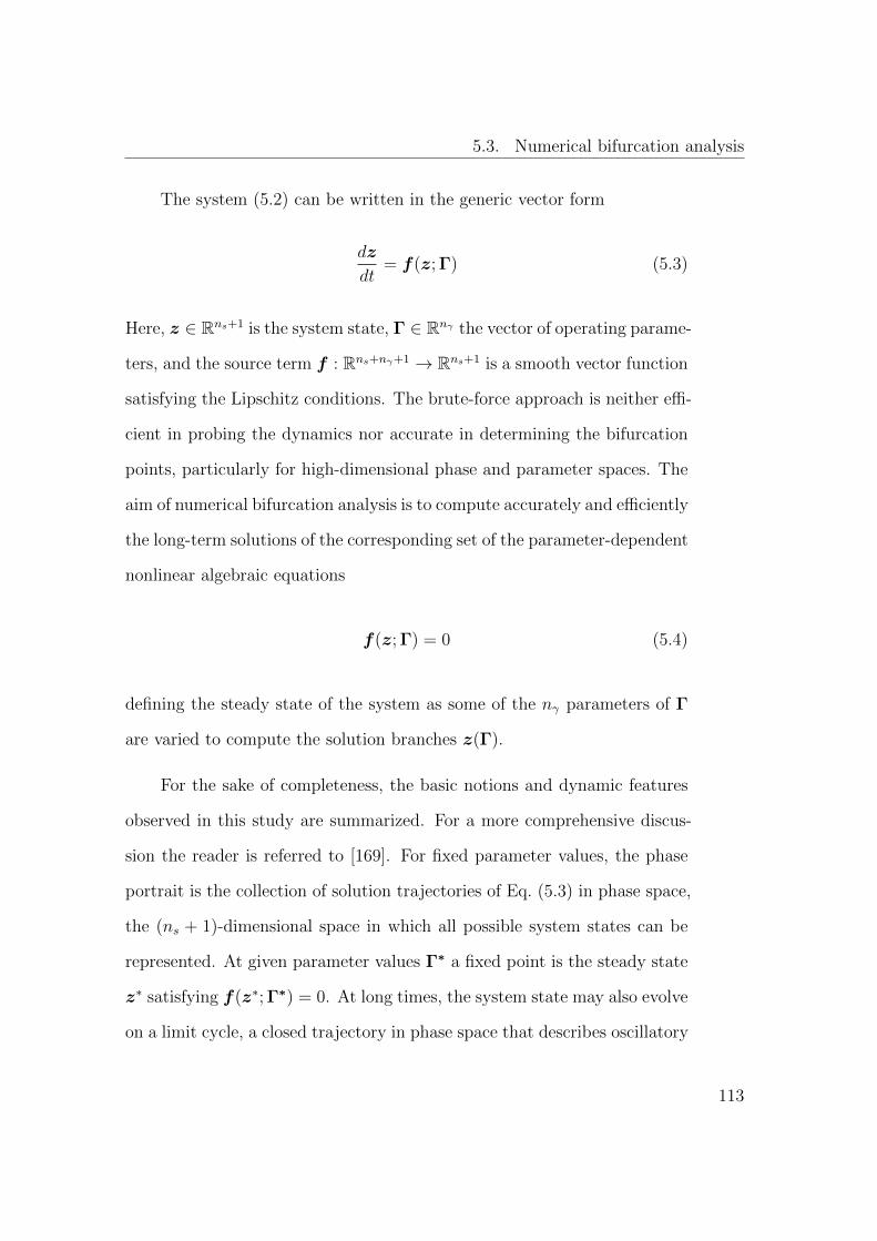
5.3. Numerical bifurcation analysis
The system (5.2) can be written in the generic vector form
dz
dt= f(z; Γ) (5.3)
Here, z ∈ Rns+1 is the system state, Γ ∈ Rnγ the vector of operating parame-
ters, and the source term f : Rns+nγ+1 → Rns+1 is a smooth vector function
satisfying the Lipschitz conditions. The brute-force approach is neither effi-
cient in probing the dynamics nor accurate in determining the bifurcation
points, particularly for high-dimensional phase and parameter spaces. The
aim of numerical bifurcation analysis is to compute accurately and efficiently
the long-term solutions of the corresponding set of the parameter-dependent
nonlinear algebraic equations
f(z; Γ) = 0 (5.4)
defining the steady state of the system as some of the nγ parameters of Γ
are varied to compute the solution branches z(Γ).
For the sake of completeness, the basic notions and dynamic features
observed in this study are summarized. For a more comprehensive discus-
sion the reader is referred to [169]. For fixed parameter values, the phase
portrait is the collection of solution trajectories of Eq. (5.3) in phase space,
the (ns + 1)-dimensional space in which all possible system states can be
represented. At given parameter values Γ∗ a fixed point is the steady state
z∗ satisfying f(z∗; Γ∗) = 0. At long times, the system state may also evolve
on a limit cycle, a closed trajectory in phase space that describes oscillatory
113

5. n-heptane/air complex dynamics
behavior. Together with fixed points they are the most commonly observed
types of limit sets. If the qualitative structure of the phase portrait changes
at Γ = Γ∗ then a bifurcation occurs, and (z∗; Γ∗) defines the bifurcation
point. The bifurcation diagram is the plot of some function of the state
variable z at the limit set as a function of one or more components of the
controlling parameters Γ.
The local stability of a state can be characterized by eigenvalues and
eigenvectors of the Jacobian matrix of the source term of (5.3), J = ∂f∂z
[161,169]. As the solution branch Γ is followed during variation of a single
parameter, the eigenvalues follow trajectories when the real part is plotted
vs the imaginary part on the complex plane, and bifurcations occur when
the eigenvalue acquires a zero real part. In the generic case, when a real
eigenvalue crosses zero at (zTP ; ΓTP ), two fixed points collide and disap-
pear and the (zTP ; ΓTP ) is a turning point bifurcation. When a complex
pair of eigenvalues crosses the imaginary axis at (zHB; ΓHB), a stable state
loses stability and in the generic case a limit cycle is born. It can be shown
that these co-dimension one bifurcation points (i.e. obtained by varying a
single parameter) follow curves when a second parameter is varied simulta-
neously which can meet or cross at co-dimension two points. These higher
co-dimension bifurcations play the role of organizing centers of lower-order
bifurcations [169]. At a cusp bifurcation two turning point curves meet tan-
gentially and the parameter space is divided into regions having different
number of steady states. At a Bogdanov-Takens bifurcation, the lineariza-
tion at the fixed point has a pair of real zero eigenvalue and satisfies some
114

5.4. Validation of skeletal mechanism for complex dynamics
technical non-degeneracy conditions [169]. At a double Hopf or Hopf-Hopf
point the Jacobian has two pairs of purely imaginary eigenvalues.
The package AUTO-07p [162, 163] is used for the continuation and
bifurcation analysis of the system of equations (5.2). In the combustion
community, AUTO has been used to study the dynamics of the Belousov-
Zhabotinsky reaction [170] and for hydrogen/air mixtures in PSRs [154,156].
In order to perform a comprehensive study of n-heptane in a PSR, AUTO-
07p was coupled with the CHEMKIN library [104] so that complex reaction
mechanisms can be readily accommodated.
Dynamical system analysis for high hydrocarbons is less common and
the recent studies have mostly focused on the effect of varying the residence
time on the reactor temperature [157–159]; the details of the employed
continuation approach were not provided.
5.4 Validation of skeletal mechanism for n-h-
eptane/air mixture for complex dynamics
A skeletal mechanism R161 which was validated for a wide range of ther-
modynamic conditions for auto-ignition in a constant pressure laminar pre-
mixed flames in chapter 4 ( [107]) is considered.
Careful inspection of the results of time integration in a transient PSR
revealed that 13 intermediate species that participate in important reactions
appear only as reactants in irreversible reactions in the detailed mechanism.
Since they cannot be produced, their concentration remains identically zero
115

5. n-heptane/air complex dynamics
and they can be safely removed to produce a skeletal n-heptane mechanism
with 149 species in 669 reactions, referred to R149.
Continuation with respect to the residence time for a stoichiometric
mixture of n-heptane and air with T0 = 650 K and p = 1, 5 and 20 atm is
shown in Fig. 5.2. Although not marked in the figure, the skeletal mecha-
nism is able to capture accurately not only the turning but also the Hopf
bifurcation points (table 5.1), which will be discussed in Sec. 5.6. It can
Table 5.1: Comparison of the bifurcation points computed with the detailed(D561) and the skeletal (R149) mechanisms; TPi and HB1 are as markedin Fig. 5.3 (adiabatic PSR at T0 = 650 K, ϕ = 1).
p TP1 TP2 TP3 HB1
[atm] (τ [s], T [K]) (τ [s], T [K]) (τ [s], T [K]) (τ [s], T [K])D561 1 (2.32× 10⁻⁵, 1735.4) (1.02,790.2) (1.22× 10⁻³, 706.5) (1.04× 10⁻², 741.9)
5 (6.35× 10⁻⁶, 1846.1) (6.38× 10⁻², 840.3) (4.75× 10⁻⁴, 749.6) (3.13× 10⁻³, 789.0)20 (2.78× 10⁻⁶, 1981.4) (7.24× 10⁻³, 889.0) (2.37× 10⁻⁴, 789.9) (9.21× 10⁻⁴, 833.8)
D149 1 (2.33× 10⁻⁵, 1739.2) (1.08, 807.3) (8.41× 10⁻⁴, 717.3) (6.98× 10⁻³, 756.5)5 (6.39× 10⁻⁶, 1849.5) (7.34× 10⁻², 859.5) (3.76× 10⁻⁴, 760.1) (2.29× 10⁻³, 803.2)20 (2.81× 10⁻⁶, 1983.8) (8.93× 10⁻³, 908.4) (2.24× 10⁻⁴, 800.3) (7.09× 10⁻⁴, 844.7)
therefore be concluded that the skeletal mechanism provides an accurate de-
scription of the kinetics and retains high fidelity to the complex non-linear
dynamics of n-heptane oxidation in comparison to the detailed mechanism.
5.5 CSP analysis
The processes contributing to the dominant time scale at the bifurcation
points are investigated in Sec. 5.6 via algorithmic tools provided by the
Computational Singular Perturbation.
116

5.5. CSP analysis
τ [s]
T[K
]
106
105
104
103
102
101
100
750
1000
1250
1500
1750
2000
2250
2500
2750
p =1 a
tmp =5 a
tmp =20
atm
Figure 5.2: Comparison of the dependence of reactor temperature on theresidence time for an adiabatic PSR at T0 = 650 K, ϕ = 1.0 and variouspressures using the detailed (solid lines) and skeletal (open circles) reactionmechanisms.
The system of equations (5.2) for an adiabatic PSR can be rewritten
as
dz
dt= g(z) = P (z) +L(z) (5.5)
by decomposing the right hand side in terms of the chemical source term
P (z)
P =
[W1ω1
ρ, · · ·Wnsωns
ρ,−∑ns
i=1Wiωihiρcp
]T
(5.6)
and the flow term L(z)
L =
[Y 0
1 − Y1
τ, · · · , Y
0ns − Ynsτ
,
∑nsi=1 Y
0i (h0
i − hi)cpτ
]T
(5.7)
117
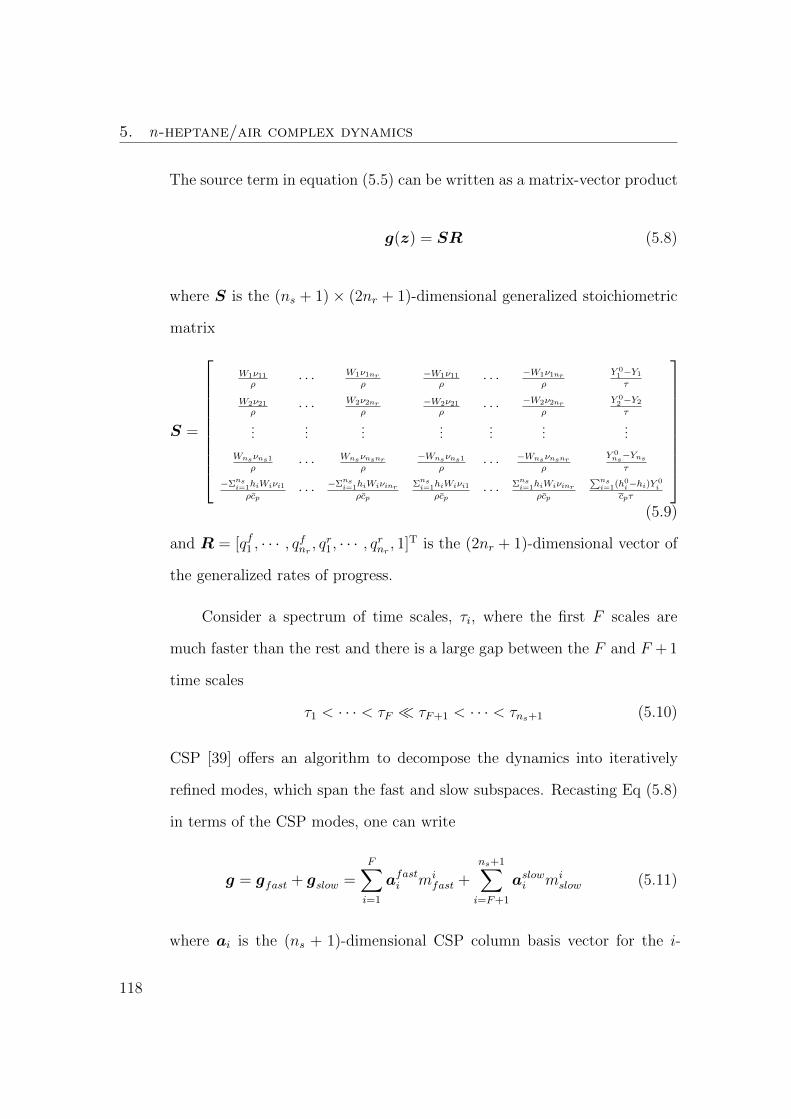
5. n-heptane/air complex dynamics
The source term in equation (5.5) can be written as a matrix-vector product
g(z) = SR (5.8)
where S is the (ns + 1)× (2nr + 1)-dimensional generalized stoichiometric
matrix
S =
W1ν11ρ
· · · W1ν1nrρ
−W1ν11ρ
· · · −W1ν1nrρ
Y 01 −Y1τ
W2ν21ρ
· · · W2ν2nrρ
−W2ν21ρ
· · · −W2ν2nrρ
Y 02 −Y2τ
......
......
......
...
Wnsνns1ρ
· · · Wnsνnsnrρ
−Wnsνns1ρ
· · · −Wnsνnsnrρ
Y 0ns−Ynsτ
−Σnsi=1hiWiνi1ρcp
· · · −Σnsi=1hiWiνinrρcp
Σnsi=1hiWiνi1ρcp
· · · Σnsi=1hiWiνinrρcp
∑nsi=1(h0i−hi)Y 0
i
cpτ
(5.9)
and R = [qf1 , · · · , qfnr , qr1, · · · , qrnr , 1]T is the (2nr + 1)-dimensional vector of
the generalized rates of progress.
Consider a spectrum of time scales, τi, where the first F scales are
much faster than the rest and there is a large gap between the F and F + 1
time scales
τ1 < · · · < τF τF+1 < · · · < τns+1 (5.10)
CSP [39] offers an algorithm to decompose the dynamics into iteratively
refined modes, which span the fast and slow subspaces. Recasting Eq (5.8)
in terms of the CSP modes, one can write
g = gfast + gslow =F∑i=1
afasti mifast +
ns+1∑i=F+1
aslowi mislow (5.11)
where ai is the (ns + 1)-dimensional CSP column basis vector for the i-
118

5.5. CSP analysis
th mode with amplitude mi = bi · g. The complementary vector space
element bi is the CSP row basis vector satisfying orthogonality condition
(written in Kronecker form) bi ·aj = δij. Typically the F fastest time scales
are dissipative, the corresponding CSP modes quickly become exhausted
and the system state evolves on the slow subspace, which can then be
approximated by
mifast ≈ 0 i = 1, · · · , F (5.12)
The relaxation on the slow subspace is then governed by
dz
dt≈ gslow (5.13)
Local information for the system time scales can be obtained from Jg, the
Jacobian of g. For real eigenvalues (complex pairs are treated as described
in [112]), the CSP i-th mode can be distinguished with a time scale approx-
imated by τ ≈ |λi|−1, the i-th eigenvalue of Jg [171]. To leading order CSP
vectors can be approximated by the right and left eigenvectors, i.e. ai = vi
and bi = vTi [171], as they defined in chapter 2.
The decomposition approach presented above, leads to the introduc-
tion of different diagnostic tools to quantify the contribution of species and
reactions or other processes to the CSP mode of interest. The i-th CSP
mode can be characterized based on the sign of Re(λi), the real part of
the eigenvalue of Jg. The CSP mode related to the positive or less nega-
tive eigenvalue plays the main role in limiting phenomena like ignition and
extinction [157–159,172–174].
119

5. n-heptane/air complex dynamics
The contribution of process k to the amplitude of the i-th CSP mode
can be computed with the help of the amplitude participation index [39,159,
164,166]
APIik =(vi
T · Sk)Rk∑2nr+1k′=1 |(viT · Sk′)Rk′|
(5.14)
where k = 1, · · ·nr and k = nr + 1, · · · , 2nr correspond to the contribution
of the forward and reverse reaction rates and k = 2nr+1 to the contribution
of flow term. The API values are normalized to [0, 1] and complex conjugate
pairs of modes can be transformed into a pair of real modes as described
in [112,164].
The Jacobian matrix Jg can be decomposed based on the contribution
of the processes,
Jg =2nr+1∑k=1
ck (5.15)
where the ck = ∇(SkRk) is the (ns + 1)× (ns + 1)-dimensional gradient of
the vector SkRk. The i-th eigenvalue of Jg can then be written as,
λi = vTi · c1vi + · · ·+ vT
i · c2nr+1vi (5.16)
and the normalized contribution of process k to the value of the i-th eigen-
value (i-th time scale) defines the timescale participation index [34,158,171,
175],
TPIik =vTi · ckvi∑2nr+1
k′=1 |vTi · ck′vi|
(5.17)
The analytic Jacobian matrix used in the CSP analysis is obtained by apply-
ing the automatic differentiation tool Tapenade [176] on the source code of
120

5.6. Continuation and bifurcation analysis
the transient PSR, and the eigenvalues and the left and right eigenvectors of
the Jacobian were computed using LAPACK routines [177]. In the following,
we will only analyze the mode corresponding to the leading eigenvalue, i.e.
the one with positive or least negative real part, to identify the dominant
process and reactions for ignition, extinction and oscillatory behavior.
In addition to the time scale analysis, entropy production, plays an
important role in characterizing the reversibility of the system [178].
Chemical affinity, Gibbs free energy and entropy production are closely
related [130,131]. The reactions which contribute more in the production of
entropy are responsible for relaxing the system from the initial state towards
the maximum entropy state (equilibrium) and can be ranked accordingly
(see for example [179] for a combustion application). In this work, entropy
production analysis will be applied at bifurcation points to identify the
reactions which are responsible for combustion irreversibility.
5.6 Continuation and bifurcation analysis
In this section, the effect of the variation of the system parameters on the dy-
namics of n-heptane/air mixtures in adiabatic and non-adiabatic perfectly
stirred reactors are investigated using AUTO-07p [163].
121

5. n-heptane/air complex dynamics
10-6
10-5
10-4
10-3
10-2
10-1
100
τ [s]
600
800
1000
1200
1400
1600
1800
2000
2200
2400
2600
T [
K]
TP4
TP1
TP2
HB1
HB2
TP3
S1
HB1HB
2
TP3
TP4
10-3
700
800
strongly burning
unstable branch
cool flameextinguished
(a)
-400 -300 -200 -100 0 100 200 300
Re(λ)
-3000
-2000
-1000
0
1000
2000
3000
Im(λ)
HB1
HB2
HB2
HB1
TP3
(b)
Figure 5.3: (a) Reactor temperature as a function of residence time fora stoichiometric n-heptane/air mixture (p = 1 atm, T0 = 700 K) in anadiabatic PSR. Solid (dashed) lines indicate stable (unstable) states, whilethe solid curves between HB1 and HB2 of the expanded inset show themaximum and minimum reactor temperatures during the oscillations. (b)Trajectories of the leading eigenvalues along the cool flame branch for τ <6× 10⁻³s.
122
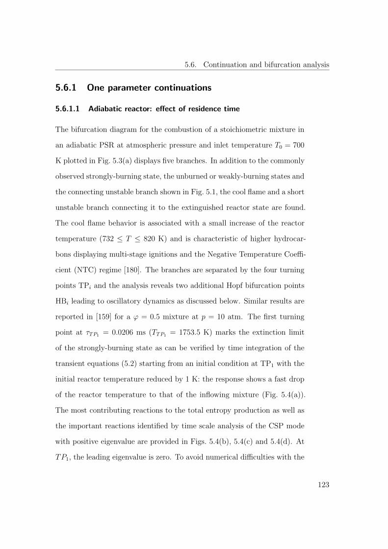
5.6. Continuation and bifurcation analysis
5.6.1 One parameter continuations
5.6.1.1 Adiabatic reactor: effect of residence time
The bifurcation diagram for the combustion of a stoichiometric mixture in
an adiabatic PSR at atmospheric pressure and inlet temperature T0 = 700
K plotted in Fig. 5.3(a) displays five branches. In addition to the commonly
observed strongly-burning state, the unburned or weakly-burning states and
the connecting unstable branch shown in Fig. 5.1, the cool flame and a short
unstable branch connecting it to the extinguished reactor state are found.
The cool flame behavior is associated with a small increase of the reactor
temperature (732 ≤ T ≤ 820 K) and is characteristic of higher hydrocar-
bons displaying multi-stage ignitions and the Negative Temperature Coeffi-
cient (NTC) regime [180]. The branches are separated by the four turning
points TPi and the analysis reveals two additional Hopf bifurcation points
HBi leading to oscillatory dynamics as discussed below. Similar results are
reported in [159] for a ϕ = 0.5 mixture at p = 10 atm. The first turning
point at τTP1 = 0.0206 ms (TTP1 = 1753.5 K) marks the extinction limit
of the strongly-burning state as can be verified by time integration of the
transient equations (5.2) starting from an initial condition at TP1 with the
initial reactor temperature reduced by 1 K: the response shows a fast drop
of the reactor temperature to that of the inflowing mixture (Fig. 5.4(a)).
The most contributing reactions to the total entropy production as well as
the important reactions identified by time scale analysis of the CSP mode
with positive eigenvalue are provided in Figs. 5.4(b), 5.4(c) and 5.4(d). At
TP1, the leading eigenvalue is zero. To avoid numerical difficulties with the
123
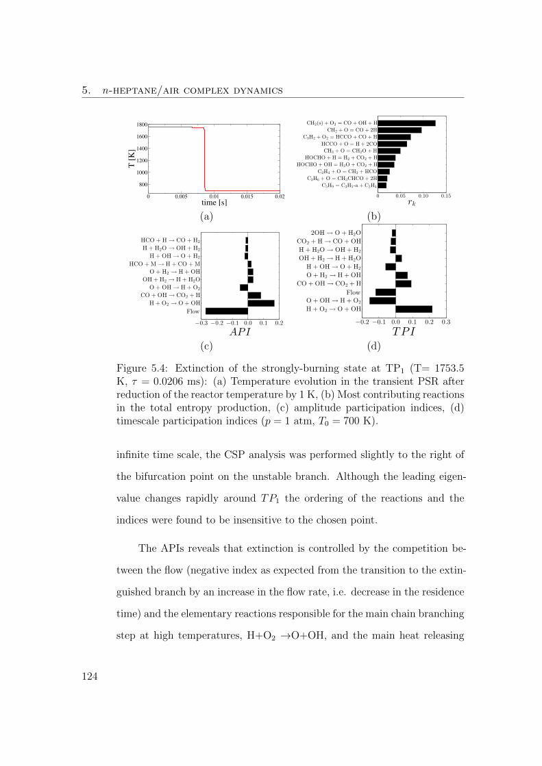
5. n-heptane/air complex dynamics
0 0.005 0.01 0.015 0.02
time [s]
800
1000
1200
1400
1600
1800
T [
K]
0 0.05 0.10 0.15
C5H9 = C3H5-a + C2H4
C3H6 + O = CH3CHCO + 2H
C2H4 + O = CH3 + HCO
HOCHO + OH = H2O + CO2 + H
HOCHO + H = H2 + CO2 + H
CH3 + O = CH2O + H
HCCO + O = H+ 2CO
C3H2 + O2 = HCCO + CO + H
CH2 + O = CO + 2H
CH2(s) + O2 = CO + OH+ H
rk
(a) (b)
−0.3 −0.2 −0.1 0.0 0.1 0.2
Flow
H + O2 → O + OH
CO + OH → CO2 + H
O + OH → H+ O2
OH + H2 → H+ H2O
O + H2 → H+ OH
HCO +M → H+ CO +M
H+ OH → O + H2
H + H2O → OH+ H2
HCO + H → CO + H2
API
−0.2 −0.1 0.0 0.1 0.2 0.3
H + O2 → O + OH
O + OH → H+ O2
Flow
CO + OH → CO2 + H
O + H2 → H+ OH
H + OH → O + H2
OH + H2 → H+ H2O
H + H2O → OH+ H2
CO2 + H → CO + OH
2OH → O + H2O
TPI
(c) (d)
Figure 5.4: Extinction of the strongly-burning state at TP1 (T= 1753.5K, τ = 0.0206 ms): (a) Temperature evolution in the transient PSR afterreduction of the reactor temperature by 1 K, (b) Most contributing reactionsin the total entropy production, (c) amplitude participation indices, (d)timescale participation indices (p = 1 atm, T0 = 700 K).
infinite time scale, the CSP analysis was performed slightly to the right of
the bifurcation point on the unstable branch. Although the leading eigen-
value changes rapidly around TP1 the ordering of the reactions and the
indices were found to be insensitive to the chosen point.
The APIs reveals that extinction is controlled by the competition be-
tween the flow (negative index as expected from the transition to the extin-
guished branch by an increase in the flow rate, i.e. decrease in the residence
time) and the elementary reactions responsible for the main chain branching
step at high temperatures, H+O2 →O+OH, and the main heat releasing
124

5.6. Continuation and bifurcation analysis
reaction, CO+OH →CO2+H (positive indices indicating that an increase
in the rates of these reactions will favor the strongly-burning state). The
dominant time scale at the chosen point (τ1 = 1/λ1 = 6.97 × 10⁻⁴ s) is
determined by the main chain branching reaction (positively in the radical-
producing direction, negatively in the reverse direction) and negatively by
the colder inflow. The main heat releasing step together with the secondary
chain branching step O+H2 →H+OH have a positive contribution. Entropy
production and thus irreversibility is dominated by reactions including small
molecules.
0 0.1 0.2 0.3 0.4 0.5
time [s]
800
1000
1200
1400
1600
1800
2000
2200
2400
2600
T [
K]
0 0.01 0.02 0.03 0.04 0.05
CH2CHO + O2 = CH2O + CO + OH
C7H14OOH1-3 = C7H14O1-3 + OH
nC7H16 + OH = C7H15-2 + H2O
nC7H16 + OH = C7H15-3 + H2O
C7H14OOH3-5 = C7H14O3-5 + OH
HCO + O2 = CO + HO2
C7H14OOH2-4 = C7H14O2-4 + OH
C2H3 + O2 = CH2O + HCO
C7H14OOH3-6 = C7H14O2-5 + OH
C7H14OOH2-5 = C7H14O2-5 + OH
rk
(a) (b)
−0.2 −0.1 0.0 0.1
Flow
H2O2(+M) → 2OH(+M)
2HO2 → H2O2 + O2
CH2O + HO2 → HCO + H2O2
2HO2 → H2O2 + O2
C7H15O2-2 → C7H14OOH2-4
C7H15-2 → pC4H9 + C3H6
C7H15-2 + O2 → C7H15O2-2
CH2O + OH → HCO + H2O
C7H15O2-2 → C7H15-2 + O2
API
−0.1 0.0 0.1 0.2
H2O2(+M) → 2OH(+M)Flow
CH2O + HO2 → HCO + H2O2
C7H15-2 → pC4H9 + C3H6
CH2O + OH → HCO + H2O
C2H3 + O2 → CH2CHO + O
2HO2 → H2O2 + O2
C7H15-4 → C2H5 + C5H10-1
CH3 + HO2 → CH4 + O2
C2H3 + O2 → CH2O + HCO
TPI
(c) (d)
Figure 5.5: Ignition of the cool flame at TP2 (T= 820.3 K, τ = 0.7571 s):(a) Temperature evolution in the transient PSR after increasing the reactortemperature by 1 K, (b) Most contributing reactions in the total entropyproduction, (c) amplitude participation indices, (d) timescale participationindices (p = 1 atm, T0 = 700 K).
The second turning point at τTP2 = 0.7571 s (TTP2 = 820.3 K) marks
125

5. n-heptane/air complex dynamics
the ignition conditions towards the strongly-burning state. Indeed, a 1
K increase of the initial reactor temperature from the conditions at TP2
results in a jump to the strongly-burning state (Fig. 5.5(a)). Entropy pro-
duction analysis reveals that reactions responsible for the breakup of heavy
molecules are most important with respect to irreversibility (Fig. 5.5(b)).
CSP analysis performed slightly to the left of TP2 on the unstable branch
(Figs. 5.5(c) and (d)) shows the clearly dominant role of the reaction H2O2 →2OH,
the main branching step at low temperature [181], both in the amplitude
and in the time scale (τ1 = 6.09 s) of the leading eigenmode. Flow has
again a negative contribution. Similar findings are reported in [164,165] for
autoignition of stoichiometric n-heptane/air mixtures in a constant volume
batch reactor at 850 K and 13.5 bar.
Along the cool flame branch, the segment connecting the two super-
critical Hopf bifurcation points HB1 and HB2 (dashed line in the inset of
Fig. 5.3(a), with the solid lines marking the oscillation amplitude) defines
the range of residence times for which the n-heptane cool flames exhibit
oscillatory behavior. The trajectories of the complex pair of eigenvalues
on the complex plain (imaginary part plotted against the real part) as τ is
decreased from τ = 6 ms along the cool flame branch of Fig. 5.3(b) show
the two crossings of the real axis at the Hopf bifurcation points HB1 and
HB2, their meeting at τ = 4.13 ms to become real, and their subsequent
trajectories along the real axis. One of them crosses to positive values at
τTP3 .
The time history of the state initialized at point S1 (τ = 0.7412 ms,
126

5.6. Continuation and bifurcation analysis
T = 760.84 K, Fig. 5.3(a)) shows the evolution to a limit cycle with a fre-
quency of about 240 Hz (Fig. 5.6(a)). At the unstable steady state S1, the
kinetics are determined by the set of reactions shown in Figs. 5.6(b), (c)
and (d). Reactions containing heavy molecules are most-contributing in the
total entropy production. The APIs show that the dominant reactions are
the dehydrogenation of n-heptane by hydroxyl radicals to produce different
isomers of the heptyl radical C7H15 and initiate the formation of the radical
pool, while the flow term has the main negative contribution. In addi-
tion, ketohydroperoxide molecules are formed from isomerization of peroxy-
alkylhydroperoxide radicals. The real part of the dominant eigenvalue at S1
is positive. The TPI shows that the slowest timescale of the unstable state
at S1 (τ1 = 4.51× 10⁻³ s) is due to the reactions CH2O+OH→HCO+H2O
and HO2+OH→H2O. At this point, flow has a contribution only on API,
which is positively affected by the H abstraction reactions by the hydroxyl
radical. As shown in [182] for a simple glycolysis model, CSP analysis can
be used to identify the processes controlling the oscillatory behavior. For
the high-dimensional n-heptane combustion, such a study is significantly
more complicated and beyond the scope of this work.
The steady cool flame becomes stable for a narrow interval when τ <
τHB2 , and eventually disappears for a shorter residence time at the third
turning point TP3 (τ = 0.413 ms, T = 731.72 K, Fig. 5.3(a)). As shown in
Fig. 5.7(a), a reactor initialized at a temperature slightly lower than TTP3
evolves towards the inlet temperature; TP3 corresponds to the first stage
ignition point of n-heptane/air mixtures. The explosive mode amplitude
127
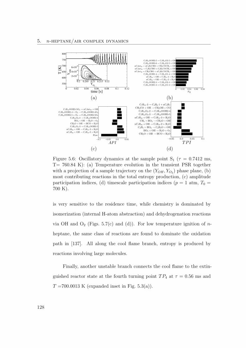
5. n-heptane/air complex dynamics
0 0.02 0.04 0.06 0.08 0.1 0.12
time [s]
550
600
650
700
750
800
T [
K]
0.2 0.205 0.21 0.215 0.22Y
O2
0
2×10⁻⁶
4×10⁻⁶
6×10⁻⁶
YO
H
0 0.02 0.04 0.06 0.08
C7H14OOH1-3 = C7H14O1-3 + OH
C7H14OOH2-4 = C7H14O2-4 + OH
nC7H16 + OH = C7H15-2 + H2O
nC7H16 + OH = C7H15-3 + H2O
C7H14OOH1-4 = C7H14O1-4 + OH
nC7ket42 = CH3CHO + nC3H7COCH2 + OH
nC7ket35 = C2H5CHO + C2H5COCH2 + OH
nC7ket24 = nC3H7CHO + CH3COCH2 + OH
C7H14OOH3-6 = C7H14O2-5 + OH
C7H14OOH2-5 = C7H14O2-5 + OH
rk
(a) (b)
−0.1 −0.05 0.0 0.05
Flow
nC7H16 + OH → C7H15-2 + H2O
nC7H16 + OH → C7H15-3 + H2O
C7H15O2-3 → C7H14OOH3-5
CH2O + OH → HCO + H2O
HO2 + OH → H2O + O2
C7H15O2-2 → C7H14OOH2-4
C7H14OOH3-5 + O2 → C7H14OOH3-5O2
C7H14OOH2-4 + O2 → C7H14OOH2-4O2
C7H14OOH3-5O2 → nC7ket35 + OH
API
−0.05 0.0 0.05 0.1
CH2O + OH → HCO + H2O
HO2 + OH → H2O + O2
C2H5 + HO2 → C2H5O + OH
nC7H16 + OH → C7H15-2 + H2O
CH3 + HO2 → CH3O + OH
nC7H16 + OH → C7H15-3 + H2O
C7H15O2-3 → C7H14OOH3-5
C7H15O2-2 → C7H14OOH2-4
CH2CO + OH → CH2OH + CO
C7H15-3 → C4H8-1 + nC3H7
TPI
(c) (d)
Figure 5.6: Oscillatory dynamics at the sample point S1 (τ = 0.7412 ms,T= 760.84 K): (a) Temperature evolution in the transient PSR togetherwith a projection of a sample trajectory on the (YOH , YO2) phase plane, (b)most contributing reactions in the total entropy production, (c) amplitudeparticipation indices, (d) timescale participation indices (p = 1 atm, T0 =700 K).
is very sensitive to the residence time, while chemistry is dominated by
isomerization (internal H-atom abstraction) and dehydrogenation reactions
via OH and O2 (Figs. 5.7(c) and (d)). For low temperature ignition of n-
heptane, the same class of reactions are found to dominate the oxidation
path in [137]. All along the cool flame branch, entropy is produced by
reactions involving large molecules.
Finally, another unstable branch connects the cool flame to the extin-
guished reactor state at the fourth turning point TP4 at τ = 0.56 ms and
T =700.0013 K (expanded inset in Fig. 5.3(a)).
128
5.6. Continuation and bifurcation analysis
0 0.005 0.01 0.015 0.02 0.025 0.03
time [s]
690
700
710
720
730
740
T [
K]
0 0.02 0.04 0.06 0.08
C7H14OOH3-5O2 = nC7ket35 + OH
C7H14OOH2-4O2 = nC7ket24 + OH
C7H14OOH1-4 = C7H14O1-4 + OH
nC7ket42 = CH3CHO + nC3H7COCH2 + OH
nC7H16 + OH = C7H15-2 + H2O
nC7H16 + OH = C7H15-3 + H2O
nC7ket35 = C2H5CHO + C2H5COCH2 + OH
nC7ket24 = nC3H7CHO + CH3COCH2 + OH
C7H14OOH3-6 = C7H14O2-5 + OH
C7H14OOH2-5 = C7H14O2-5 + OH
rk
(a) (b)
−0.3 −0.2 −0.1 0.0 0.1
Flow
C7H15O2-2 → C7H14OOH2-4
C7H15O2-3 → C7H14OOH3-5
C7H15O2-4 → C7H14OOH4-2
nC7H16 + OH → C7H15-2 + H2O
C7H14OOH2-4 + O2 → C7H14OOH2-4O2
C7H14OOH3-5 + O2 → C7H14OOH3-5O2
C7H15O2-1 → C7H14OOH1-3
C7H14OOH1-3O2 → nC7ket13 + OH
C7H14OOH2-4O2 → nC7ket24 + OH
API
−0.1 −0.05 0.0 0.05 0.1
Flow
C7H15O2-2 → C7H14OOH2-4
C7H15O2-3 → C7H14OOH3-5
HO2 + OH → H2O + O2
CH2O + OH → HCO + H2O
C7H15O2-4 → C7H14OOH4-2
nC7H16 + OH → C7H15-2 + H2O
pC4H9O2 → C4H8OOH1-3
nC7ket24 → nC3H7CHO + CH3COCH2 + OH
C7H14OOH2-4 + O2 → C7H14OOH2-4O2
TPI
(c) (d)
Figure 5.7: Cool flame extinction limit TP3 (T= 731.72 K, τ = 0.413 ms):(a) Temperature evolution in the transient PSR after decreasing the reactortemperature by 1 K, (b) most contributing reactions in the total entropyproduction, (c) amplitude participation indices, (d) time scale participationindices (p = 1 atm, T0 = 700 K).
5.6.1.2 Adiabatic reactor: effect of equivalence ratio
According to Fig. 5.3(a), the stoichiometric mixture in a PSR with τ = 1
ms can support three steady states with reactor temperatures equal to 2219
K (stable, strongly-burning), 1296 K (unstable intermediate state) and 765
K (unstable cool flame), and one stable oscillatory state around the cool
flame. The effect of the variation of ϕ on the reactor temperature is shown
in Fig. 5.8. Three branches can again be seen, but the bifurcation diagram
in this case displays an isola containing the stable strongly-burning state
and the unstable branch within the flammability range 0.325 ≤ ϕ ≤ 2.582,
which is not connected to the cool flame branch. The maximum temperature
of the strongly-burning state occurs slightly on the rich side of the fuel
129

5. n-heptane/air complex dynamics
equivalence ratio ϕ, as expected from the off-stoichiometric peak of the
adiabatic flame temperature for hydrocarbon/air mixtures [146]. The isola
is clearly separated from the cool flame branch which extends over the
whole range of ϕ with temperatures T0 ≤ T ≤ 793.8 K. Since for ϕ ≥ 2.582
the cool flame is the only steady reactor state, its kinetics can be isolated
and effectively studied. The changes in the bifurcation diagram that lead
0 0.5 1 1.5 2 2.5 3 3.5 4 4.5 5 5.5 6 6.5 φ
800
1000
1200
1400
1600
1800
2000
2200
2400
T [
K]
strongly-burning
unstable
unstable cool flame
HB1
T = 2219 K
T = 1296 K
T = 765 KHB
2oscillatory cool flame
TP2
TP1
Figure 5.8: Dependence of the reactor temperature on equivalence ratio forthe adiabatic PSR at p = 1 atm, T0 = 700 K and τ = 1 ms. Solid (dashed)lines indicate stable (unstable) steady states.
to the formation of the isola as the residence time is varied are shown in
Fig. 5.9. The isola exist for τ ≤ 0.1 s (Fig. 5.9(c)), but disappear for
τ = 0.2 s (Fig. 5.9(b)) after the unstable and the cool flame branch merge
at some intermediate residence time. For τ = 1 s the bistability region
shrinks to 0.172 ≤ ϕ ≤ 0.775, and at long enough residence times the T −ϕ
130

5.6. Continuation and bifurcation analysis
diagram will assume the familiar shape of the adiabatic flame temperature
vs. equivalence ratio curve [146]. At low residence times the size of the isola,
and with it the flammability range, decrease and at sufficiently low τ the
cool flame branch disappears (reactor temperature equal to T0, Fig. 5.9(f)).
0 1 2 3 4 5
800
1200
1600
2000
2400
T [
K]
0 2 4 6 8 10
800
1200
1600
2000
2400
0 3 6 9 12 15
800
1200
1600
2000
2400
T [
K]
0 2 4 6 8
800
1200
1600
2000
2400
0 0.5 1 1.5 2 2.5 3
φ
800
1200
1600
2000
2400
T [
K]
0.4 0.8 1.2 1.6 2
φ
800
1200
1600
2000
2400
τ = 1 s
τ = 10−1
s
τ = 10−3
s τ = 10−4
s
τ = 10−2
s
τ = 0.2 s
(a)
(e)
(c)
(f)
(d)
(b)
Figure 5.9: The dependence of temperature reactor on the equivalence ratioin the adiabatic PSR with T0 = 700 K and p = 1 atm at (a) τ = 1 s, (b)τ = 0.2 s, (c) τ = 10−1s, (d) τ = 10−2s, (e) τ = 10−3s, (f) τ = 10−4s.
5.6.1.3 Effect of heat loss
The dependence of the reactor temperature on heat loss for the stoichio-
metric mixture at atmospheric pressure and for τ = 1 s and T0 = 700 K is
depicted in Fig. 5.10. At these conditions, the adiabatic (Qloss = 0) reactor
can only operate at the strongly-burning state (T = 2463 K), but as the
131

5. n-heptane/air complex dynamics
heat loss increases the reactor temperature decreases and hysteretic behav-
ior is observed. Two turning points mark the conditions where no strongly-
burning state (TP1, Qloss = 0.67 kJ/s·m3) or cool flame (TP2, Qloss = 0.02
kJ/s·m3) can be supported in the reactor, while the existence of the Hopf
bifurcation point HB (Qloss = 0.614 kJ/s·m3, T = 1201.3 K) before TP1
indicates that the strong flame extinguishes dynamically. The solid curves
emanating from HB in the inset of Fig. 5.10 and marking the oscillation
amplitude show that the limit cycle exists for QlossHB ≤ Qloss < 0.6459
kJ/s·m3 and indicate that it is destroyed in a global bifurcation which is
difficult to locate in such a high-dimensional phase space.
0 0.1 0.2 0.3 0.4 0.5 0.6 0.7
Q.
loss[kJ/(s×m
3)]
800
1000
1200
1400
1600
1800
2000
2200
2400
T [
K]
strong flame
cool flame
HB
TP1
TP2
0.6 0.65
1000
1100
1200HB
TP1
unstable branch
Figure 5.10: The dependence of temperature reactor on heat loss in thePSR (ϕ = 1.0, T0 = 700 K, p = 1 atm and τ =1 s). Solid (dashed) linesindicate stable (unstable) branches.
132

5.6. Continuation and bifurcation analysis
The long-term behavior along the unstable branch connecting the HB
point to the TP1 point in Fig. 5.10 becomes very sensitive to the initial
condition. Fig. 5.11 shows that for Qloss = 0.646 kJ/(s×m3) starting from
two initial conditions taken along the dashed line connecting HB to TP1
in Fig. 5.10 and slightly perturbing the reactor temperature, either a multi-
period limit cycle (T = 1140 K, Fig. 5.11(a)) or extinction (T = 1137.8 K,
Fig. 5.11(b)) can be observed.
0 2 4 6 81100
1120
1140
1160
1180
1200
T [
K]
0 0.25 0.5 0.75 1 1.25 1.5
t [s]
300
600
900
1200
T [
K]
(b)
(a)
Figure 5.11: Temporal evolution of the reactor temperature for non-adiabatic PSR with Qloss = 0.646 kJ/(s×m3) (p = 1 atm, T0 = 700 K,ϕ = 1, τ = 1 s). Different initial conditions results in (a) multi-periodtransient solution for initial T = 1140 K, or (b) dynamic extinction forT = 1137.8 K.
Isolas also exist in the non-adiabatic case as shown in Fig. 5.12 for
Qloss = 0.1 kJs×m3 . Hopf bifurcation points are found along the unstable (inset
inside the isola) and the cool flame branch (inset at lower left corner). The
oscillations for τHB1 ≤ τ ≤ τTP2 have amplitudes of about 10 K and the
period increases with increasing residence time (Fig. 5.12(b)-(c), periods
133

5. n-heptane/air complex dynamics
of 0.12 and 0.17 s, respectively). Close to the turning point, the reactor
operation is characterized by long intervals (close to 70 s) of slow increase
of the temperature followed by oscillations with a period of approximately
0.3 s (Fig. 5.12(d)), indicating that the limit cycle disappears at a global
bifurcation involving the nearby saddle point [169].
10-5
10-4
10-3
10-2
10-1
100
101
τ [s]
750
1000
1250
1500
1750
2000
2250
2500
T [
K]
TP1
HB2HB
3
TP2
(a)
6.60 6.90 7.20
10
80
11
20
11
60
TP2
HB1
1×10⁻³
2×10⁻³
700
750
800
HB3
HB2
TP3
0 0.5 1 1.5 21150
1155
1160
1165
T [
K]
(b)
0 0.5 1 1.5 21100
1105
1110
1115
1120
T [
K]
(c)
0 100 200 300 400
t [s]
1084
1086
1088
1090T
[K
]
(d)
Figure 5.12: (a) Dependence of reactor temperature on residence time fornon-adiabatic PSR with Qloss = 0.1 kJ/(s×m3) (p = 1 atm, T0 = 700 K,ϕ = 1); time history of reactor temperature for (b) τ = 6.6 s, (c) τ = 7.0,(d) τ = 7.1605. Solid (dashed) lines indicate stable (unstable) branches.
5.6.2 Multi-parameter continuation
Continuation of the turning and Hopf bifurcation points while simultane-
ously varying two parameters results in bifurcation curves which delineate
regions on parameter planes with similar dynamics. For the 150-dimensional
system considered here, the two-parameter continuation with AUTO-07p
requires careful choice of the numerical parameters and the bifurcation dia-
134

5.6. Continuation and bifurcation analysis
gram had to be constructed in a piecewise manner.
5.6.2.1 Adiabatic reactor: effect of residence time and inlet mixture
temperature
We now consider the effect of the simultaneous variation of the residence
time and the inlet temperature on the four turning and the two Hopf bifur-
cation points of Fig. 5.3(a). The results are plotted in Fig. 5.13(a) together
10-6
10-5
10-4
10-3
10-2
10-1
100
τ [s]
600
800
1000
1200
1400
1600
1800
T0 [
K]
BT
TPB2
TPB1
HBB
TPB3
CP1
(a)(b)
(c)
(d)
(e)
CP2
TPB4
10-3
10-2
600
650
700
750
HBB
TPB3
BT
TPB4
CP2
10-5
10-4
10-3
10-2
10-1
100
1000
1500
2000
250010
-610
-510
-410
-310
-210
-11000
1500
2000
2500
10-4
10-2
100
τ
500
1000
1500
2000
2500
10-6
10-5
10-4
10-3
10-2
10-1
100
1600
2000
2400
2800
Figure 5.13: (a) Two-parameter (T0–τ) continuation of the turning andHopf bifurcation points of the adiabatic PSR at p = 1 atm and ϕ = 1; one-parameter bifurcation diagrams (b) for for T0 = 600 K, (c) for for T0 = 730K, (d) for for T0 = 1200 K, (e) for for T0 = 1900 K. Colors are the same asin Fig. 5.3(a).
with one-parameter diagrams at selected T0 (Figs. 5.13(b)-(e); Fig. 5.3
should also be consulted for the notation). The turning point branches
for the cool flame ignition (TPB2) and the strong state extinction (TPB1)
meet tangentially at the cusp point CP1 for an impractically short residence
time (τ, T0) = (1.9 × 10⁻⁶s, 1805.9K), and the parameter ranges between
them define the regime of multistability. To the left of the TPB1 bifurcation
135

5. n-heptane/air complex dynamics
curve and for inlet temperature lower than the TCP1 the residence time is
so low that the reactor cannot be ignited at any inlet mixture temperature.
Similarly, the turning point branches for the cool (TPB3) and the extin-
guished reactor (TPB4) states meet tangentially at the second cusp point
CP2 (τ = 2.3×10⁻⁴ s and T0 = 746.5 K), and the parameter range between
them defines the conditions for the coexistence of the two states.
For inlet temperatures higher than TCP1 = 1805.9 K, the reactor can
only operate at the strongly-burning state, irrespective of the residence time
(Fig. 5.13(e)). In the range of parameters between the bifurcation curves
TPB1 and TPB2 and the two horizontal dashed lines passing though the
CP1 and CP2, two steady (weakly- and strongly-burning states) and one
unstable steady state will be observed (Fig. 5.13(d)).
In the range between TPB1 and TPB2 and below the lower dashed line,
the dynamics become more complex, involving up to seven possible limit
sets: three steady and stable (unreacted mixture, cool and strongly-burning
state), three unstable steady states, and oscillatory cool flames. At inlet
temperature T0 = 550 K, the lower limit for which the detailed mechanism
is valid [4], one Hopf bifurcation point always exists for a residence time
between the second (TPB2) and the third (TPB3) turning points (i.e., along
the cool flame branch), as it can be seen in Fig. 5.13(b) for T0 = 600 K. It
turns out that the second Hopf point emerges from the saddle-node TPB3
locus at τ = 0.4898 s, T0 = 687.58 K. The HBB and TPB3 curves meet
tangentially at a Bogdanov-Takens (BT) bifurcation point of co-dimension
two where the steady state has a double-zero eigenvalue [169]. As the value
136

5.6. Continuation and bifurcation analysis
of inlet temperature is further increased, the turning point and the second
Hopf point, move apart and two Hopf points begin to move closer together
until finally HB1 and HB2 coalesce at the double Hopf bifurcation point
(τ, T0) = (7 × 10⁻⁴s, 719.1K), another bifurcation point of co-dimension
two, where two pairs of complex conjugate eigenvalues change their signs
simultaneously at a double Hopf bifurcation point. For 719.1 < T0 < TCP2
K, the whole cool flame branch is steady, as can be seen in Fig. 5.13(c).
As mentioned, high co-dimension points act as organizing centers for
the dynamics (see [169] for the details on the expected behavior around such
points). However, for high-dimensional systems like the one considered
here it is difficult to show the expected behavior, which includes global
bifurcations. Figure 5.14(a) shows only the transient behavior of a PSR
initialized at a residence time slightly lower than BT. The reactor state
starts to oscillate with increasing amplitude. Due to the low residence time
compared to BT point, the cool flame cannot sustain itself, it extinguishes
suddenly and the reactor temperature returns to the inlet value.
The entropy production and the CSP analysis of the mode with positive
eigenvalue at the conditions of the BT point are provided in Figs. 5.14(b),
(c) and (d).
Some of the dynamics mentioned above occurs in narrow ranges of inlet
temperatures and sometimes for very short residence times and would there-
fore be difficult to observe experimentally. Nevertheless, two-parameter
diagrams like Fig. 5.13 provide invaluable information for understanding
the combustion dynamics and to guide experiments in PSRs to parameter
137

5. n-heptane/air complex dynamics
0 0.1 0.2 0.3 0.4
time [s]
680
690
700
710
720
730
T [
K]
0 0.1 0.2 0.3727.2
727.4
727.6
727.8
728
728.2
0 0.02 0.04 0.06 0.08
C7H14OOH3-5O2 = nC7ket35 + OH
C7H14OOH2-4O2 = nC7ket24 + OH
C7H14OOH1-4 = C7H14O1-4 + OH
nC7ket42 = CH3CHO + nC3H7COCH2 + OH
nC7H16 + OH = C7H15-2 + H2O
nC7H16 + OH = C7H15-3 + H2O
nC7ket35 = C2H5CHO + C2H5COCH2 + OH
nC7ket24 = nC3H7CHO + CH3COCH2 + OH
C7H14OOH3-6 = C7H14O2-5 + OH
C7H14OOH2-5 = C7H14O2-5 + OH
rk
(a) (b)
−0.2 −0.1 0.0 0.1
Flow
C7H15O2-2 → C7H14OOH2-4
C7H15O2-3 → C7H14OOH3-5
nC7H16 + OH → C7H15-2 + H2O
C7H15O2-4 → C7H14OOH4-2
nC7H16 + OH → C7H15-3 + H2O
C7H14OOH2-4 + O2 → C7H14OOH2-4O2
nC7H16 + OH → C7H15-4 + H2O
C7H15O2-1 → C7H14OOH1-3
C7H14OOH3-5 + O2 → C7H14OOH3-5O2
API
−0.05 0.0 0.05
CH2O + OH → HCO + H2O
HO2 + OH → H2O + O2
C7H15O2-2 → C7H14OOH2-4
C7H15O2-3 → C7H14OOH3-5
nC7H16 + OH → C7H15-2 + H2O
C7H15O2-4 → C7H14OOH4-2
C2H5 + HO2 → C2H5O + OH
pC4H9O2 → C4H8OOH1-3
C7H14OOH2-4 + O2 → C7H14OOH2-4O2
C7H15O2-1 → C7H14OOH1-3
TPI
(c) (d)
Figure 5.14: The analysis of Bogdanov-Takens bifurcation point, BT (T0 =687.58 K, T = 727.89 K, τ = 0.4898 ms): (a) Temperature evolution in thetransient PSR after small perturbation in reactor temperature, (b) Mostcontributing reactions in the total entropy production, (c) Amplitude par-ticipation indices, (d) Time scale participation indices (p = 1 atm andϕ = 1).
regions where the kinetics at different regimes can be effectively probed.
Continuation with respect to additional parameters can help to identify
parameter ranges that are more amenable to experimental investigation.
5.6.2.2 Adiabatic reactor: effect of pressure and equivalence ratio on
the τ − T0 bifurcation diagram
The effect of pressure and equivalence ratio on the τ−T0 bifurcation diagram
can be studied by computing the curves for different values of p and ϕ.
At higher pressure the observed bifurcations do not change, but the
branches of the critical curves shift to lower residence times rendering the
138

5.7. Conclusions
10-7
10-6
10-5
10-4
10-3
10-2
10-1
100
τ [s]
600
800
1000
1200
1400
1600
1800
2000
T0 [
K]
solid : p = 1 atmdashed: p = 5 atm
10-6
10-5
10-4
10-3
10-2
10-1
100
τ [s]
600
800
1000
1200
1400
1600
1800
2000
T0 [
K]
solid : φ = 1
dashed : φ = 0.8
dotted : φ = 1.2
(a) (b)
Figure 5.15: Effect of (a) pressure and (b) equivalence ratio on the τ−T0 two-parameter continuation diagrams (adiabatic PSR working at stoichiometricconditions).
strongly-burning state more dominant (Fig. 5.15(a)). The range of inlet
temperatures leading to cool flame oscillations widens, but the reduction
in the range of τ make their experimental investigation more difficult. The
inlet composition is found to have only a minor effect on the dynamics
for ϕ = 0.8, 1.0, and 1.2 (Fig. 5.15(b)). Figure 5.15 can be considered as a
projection of the three-parameter bifurcation diagram on the two-parameter
space τ−T0. By repeating the analysis for different pressures or equivalence
ratios, a three-parameter diagram can be constructed.
5.7 Conclusions
The complex dynamics and bifurcations of high hydrocarbons like n-heptane
in perfectly stirred reactors can be systematically investigated using a com-
bination of time integration of the transient PSR equations and single- and
139

5. n-heptane/air complex dynamics
multi-parameter continuation and stability analysis with AUTO-07p [163].
The study is carried out with a skeletal mechanism with 149 species and
669 elementary reactions constructed by applying the proposed entropy
production analysis method (chapter 4 and [107]) on the detailed LLNL2
scheme [136] (561 species and 2539 reactions). Ignition delay time and flame
speed over an extended range of conditions and the bifurcation points in
the PSR computed with the skeletal mechanism are in very good agreement
with the results computed with the detailed mechanism.
The reactor stability was investigated with respect to the residence
time τ , inlet temperature T0, pressure p, inlet mixture equivalence ratio
ϕ and heat loss Qloss. Multiple turning and Hopf bifurcation points were
found in the continuation with respect to τ defining the bifurcation values
and showing that up to six limit sets can coexist for the same operating con-
ditions, both physically-realizable (steady and stable: extinguished reactor,
cool flames and strongly-burning state, or unsteady: cool flame oscillations)
as well as unphysical (unstable steady states along the branches connecting
either the turning points defining the conditions for ignition and extinction
or Hopf bifurcation point leading to the oscillatory dynamics). The kinetics
at the bifurcation points were analyzed with the help of the importance and
amplitude indices of Computational Singular Perturbation to identify the
important reactions for the explosive mode corresponding to the eigenvalue
with positive or least negative real part and entropy production analysis
which points to the reactions contributing most to irreversibility. Continua-
tion with respect to equivalence ratio revealed isolas, and their appearance
140

5.7. Conclusions
was studied by varying the residence time. With respect to heat loss, a
Z-shaped curve was obtained, and the extinction of the strongly-burning
reactor was found to be dynamic (oscillatory extinction). Time integra-
tion indicated that global bifurcations also play an important role in the
dynamics.
Two-parameter continuation with respect to τ and T0 revealed the
range of conditions of the different steady and oscillatory states. Co-dimension
two bifurcation point (cusp, Bogdanov-Takens and double Hopf) were found,
but the high-dimensionality of the system complicates their detailed inves-
tigation. The effect of pressure and equivalence ratio on the two-parameter
diagram was also studied. Increasing pressure for a stoichiometric mixture
in an adiabatic PSR was found to shift the critical curves to lower residence
time, but the bifurcations between different states was unaffected. Equiva-
lence ratio variations in an atmospheric pressure adiabatic PSR have only
a minor effect.
To the best of the authors’ knowledge this is the first comprehensive
and systematic study of the combustion dynamics of a high hydrocarbon
in perfectly stirred reactors. However, the complexity resulting from both
the high dimensionality of the dynamical system and the large number of
parameters hinder the exploration of all possible behaviors. A lot remains
to be done, particularly in terms of exploring different combinations of
parameters, locating and tracking global bifurcations, and analyzing the
wealth of the generated information to probe and understand the reaction
kinetics determining the critical conditions.
141

5. n-heptane/air complex dynamics
The numerically predicted ranges of different dynamics can guide ex-
perimental investigations to interesting conditions, which will provide data
for the validation or iterative refinement of detailed reaction mechanisms.
142

Chapter 6
Non-Perturbative Hydrodynamic
Limits: A case study 1
6.1 Introduction
The derivation of hydrodynamic equations from the Boltzmann kinetic equa-
tion is the classical problem of statistical mechanics. The best known tech-
nique, the Chapman-Enskog (CE) method [54], is a perturbation method
based on a small parameter (Knudsen number). While the formal deriva-
tion of the Navier-Stokes equation from the Boltzmann equation by this
method is a textbook example of the success of statistical physics, many
problems related to the hydrodynamic limit of the kinetic equations re-
main unsolved [51]. The CE perturbation expansion fails as the post-
Navier-Stokes hydrodynamic equations (e.g. Burnett’s equations) are un-
stable [183]. Moreover, even at the Navier-Stokes level, the rate of dissipa-
1The content of the present chapter is published in Karlin, I. V., Chikatamarla, S.S., & Kooshkbaghi, M. (2014). Non-perturbative hydrodynamic limits: A case study.Physica A: Statistical Mechanics and its Applications, 403, 189-194.
143
6. Non-Perturbative Hydrodynamic Limits: A case study
tion (by viscosity, thermal conductivity or diffusion) is unbounded which
contradicts the finiteness of relaxation times in the kinetic picture. Finally,
as pointed out by many authors (e.g. [184]), the smallness parameter of
the problem is not a fixed quantity (unlike, for example, the fine structure
constant in quantum electrodynamics) but can be always scaled out.
All this points at the inability of the CE method to tackle the above
problem, and non-perturbative approaches are sought. To that end, mini-
mal kinetic theories such as Grad’s finite-moment systems have been stud-
ied in detail [53, 56], including the exact summation of the entire CE se-
ries. Some results obtained along these lines are surprising. For exam-
ple, Slemrod [184] noted that exact summation of the CE expansion re-
sults in hydrodynamic equations of Korteweg’s type (that is, containing
the capillarity-type contribution) rather than a (modified) Navier-Stokes
equation. However, results for the kinetic equations, that is, for infinite mo-
ment systems remained almost entirely unexplored due to lack of analytical
non-perturbative techniques.
In this chapter, we introduce a novel analytic approach to extract non-
perturbatively the hydrodynamic component out of the kinetic equations.
We consider in detail a model kinetic equation, and derive an exact invari-
ance equation which is in striking resemblance with the Schwinger-Dyson
equation of non-perturbative field theories. Based on the exact solution to
the invariance equation, we build up a systematic non-perturbative exten-
sion procedure and show its relation to the conventional Chapman-Enskog
method. The present approach can be used beyond the model kinetic equa-
144

6.2. Non-perturbative derivation of hydrodynamic manifold
tion considered below, and we outline some further steps towards the non-
perturbative hydrodynamic limit.
6.2 Non-perturbative derivation of hydrodynamic
manifold
We consider the one-dimensional kinetic equation for the distribution func-
tion f(x, v, t):
∂tf = −v∂xf − τ−1 (f − f eq) , (6.1)
where the local equilibrium has the form
f eq = n(x, t) (2πkBT/m)−1/2 e− mv2
2kBT , (6.2)
with n(x, t) the locally conserved density,
n =
∫ ∞−∞
f(v, x, t)dv. (6.3)
and ∂t, ∂x denote differentiation with respect to time and spatial direction.
The conventional CE analysis of (6.1) is to introduce a small parameter ε:
τ → ετ , and to expand, f = f (0)+εf (1)+. . . , in order to produce a closure to
the balance equation, ∂tn = −∂xj, where j =∫∞−∞ vfdv is the density flux.
One easily computes the first two terms of the CE closure, ω(2)CE = εD∂2
x (first
approximation; this is the conventional diffusion); ω(4)CE = εD∂2
x + ε2D2∂4x
(second approximation), where D = τkBT/m is the diffusion coefficient.
The problem with such a perturbation approach is readily seen even in
145

6. Non-Perturbative Hydrodynamic Limits: A case study
the present case: After an appropriate rescaling in time and space, the
mode’s relaxation rate ω(k), where k is the wave vector, is (a) unbounded as
k →∞ in the first approximation, and (b) unstable for k > 1 in the second
approximation (Fig. 6.1). Thus, even for the simplest kinetic equation (6.1),
0 0.2 0.4 0.6 0.8 1
k
-1
-0.8
-0.6
-0.4
-0.2
0
ω^
1
2
43
Figure 6.1: Hydrodynamic limit of Eq. (6.1). Dashed line: First CE approxi-
mation, ω(2)CE = −k2 (unbounded as k →∞); Dot-dashed line: Burnett-type
approximation, ω(4)CE = −k2+k4 (unstable for k > 1); Solid and dotted Lines:
Continuation by the sequence (6.30). Curves 1, 2, 3 and 4 correspond to the
hydrodynamic branch ω(2n)H for n = 1, 2, 20, 25, respectively. Interception
by a partner kinetic mode ω(2n)P (dots) at k = k
(2n)c is indicated by open
circles.
application of the perturbative CE expansion inherits the essential problems
as in the case of the Boltzmann equation. Our goal here is to develop a
non-perturbative method to study the hydrodynamic limit of (6.1).
146

6.2. Non-perturbative derivation of hydrodynamic manifold
In the sequel we set kBT/m = 1, τ = 1. Moments of the distribution
functions can be written as
Ml(x, t) =
∫ ∞−∞
vlf(v, x, t)dv. (6.4)
Equation (6.1) is equivalent to an infinite-moment system,
∂tMl = −∂xMl+1 −Ml +M eql . (6.5)
Instead of the infinite set of moments (6.4), it proves convenient to con-
sider the generating function Z(λ, x, t) (Fourier transform in the velocity
variable),
Z =
∫ ∞−∞
e−iλvf(v, x, t)dv. (6.6)
Let us denote Z± the real and imaginary parts of Z = Z+ + iZ−; Since
moments (6.4) are real-valued, for even and odd moments we have, respec-
tively,
M2n = (−1)n(∂2nλ Z
+)λ=0
,
M2n+1 = (−1)n+1(∂2n+1λ Z−
)λ=0
.
In terms of the generating function, Eq. (6.1) is represented as a coupled
system for Z+ and Z−,
∂tZ+ = ∂x∂λZ
− − Z+ + Zeq,
∂tZ− = −∂x∂λZ+ − Z−,
(6.7)
147

6. Non-Perturbative Hydrodynamic Limits: A case study
where Zeq = n(x, t)ϕeq, and ϕeq = e−λ2
2 . Finally, applying the Fourier
transform in space, equations (6.7) become
∂tZ+ = ik∂λZ
− − Z+ + nϕeq, (6.8)
∂tZ− = −ik∂λZ+ − Z−, (6.9)
where Z±(λ, k, t) =∫∞−∞ e
−ikxZ±(λ, x, t)dx depend on the wave vector k.
Equations (6.8,6.9) are the starting point for the non-perturbative anal-
ysis. In the hydrodynamic limit, all moments depend on space and time
only through their dependence on the locally-conserved field (density). To
this end, the most general and yet unknown relation for the generating
functions Z± can be written as
Z+ = Θ+(λ, k2)n(k, t), (6.10)
Z− = ikΘ−(λ, k2)n(k, t), (6.11)
where Θ± are the functions in question, satisfying the consistency conditions,
Θ+(0, k2) = 1, Θ−(0, k2) = 0. Knowing Θ−, the balance equation becomes,
∂tn = −k2Gn, where
G = (∂λΘ−)λ=0, (6.12)
is the extended diffusion coefficient (EDC).
Let us now formulate the most general condition for Θ±. The time-
derivative of the generating function can be computed in two ways. On the
148

6.2. Non-perturbative derivation of hydrodynamic manifold
one hand, it is computed by chain rule and using the balance equation:
∂macrot Z+ =
∂Z+
∂n∂tn = (−k2GΘ+)n, (6.13)
∂macrot Z− =
∂Z−
∂n∂tn = ik(−k2GΘ−)n. (6.14)
This is the macroscopic time derivative, or the derivative of the yet unknown
closed generating function due to the (also yet unknown) closed balance
equation. On the other hand, the microscopic time derivative is given by
the right hand side of (6.8,6.9):
∂microt Z+ = (−k2∂λΘ
− − Θ+ + ϕeq)n, (6.15)
∂microt Z− = ik(−∂λΘ+ − Θ−)n. (6.16)
The dynamic invariance condition [56] requires that the micro- and the
macroscopic derivatives of the generating function should give the same
result, independently of n:
∂microt Z± = ∂macro
t Z±. (6.17)
Thus, the invariance condition for the generating function is a system of
two first-order equations,
−k2GΘ+ + k2∂λΘ− + Θ+ − ϕeq = 0, (6.18)
−k2GΘ− + ∂λΘ+ + Θ− = 0, (6.19)
149

6. Non-Perturbative Hydrodynamic Limits: A case study
subject to the initial conditions, Θ+(0, k2) = 1, Θ−(0, k2) = 0. It can be
readily checked that the invariance equation generates the CE solution when
functions Θ± are expanded into Taylor series around k2 = 0. Our goal is,
however, to solve the invariance equation avoiding any expansion of this
kind. We proceed with a few transformations: (i) Differentiate (6.18) with
respect to λ and eliminate ∂λΘ+ to get the second-order equation for Θ−:
k2∂2λΘ− − (1− k2G)2Θ− − ∂λϕeq = 0; (6.20)
(ii) Differentiate equation (6.20) one more time; use transformed variable,
∂λΘ− = Σe−λ
2/2, and note that G = (Σ)λ=0. Thus, the invariance equation
for the generating function becomes,
(k2G− 1)2Σ + (1−λ2)(k2Σ− 1)=k2(∂2λΣ− 2λ∂λΣ). (6.21)
The invariance equation (6.21) is crucial. We note that, although not form-
identical, equation (6.21) can be regarded as an analog of the basic equation
of the non-perturbative approach in quantum field theories, the Schwinger-
Dyson equation (SDE) [185, 186]. Indeed, SDE is a relationship between
the one-particle Green’s function G and the mass operator Σ. Standard
derivation of SDE proceeds along the lines similar to the above, considering
the generating function of many-particle Green’s functions. In the present
context, the “mass operator” Σ in (6.21) provides the coupling to all higher-
order moments, and self-consistently defines the EDC G. For the present
analysis of (6.21), it is convenient to introduce the frequency function Ω =
150

6.2. Non-perturbative derivation of hydrodynamic manifold
−k2Σ, so that ω = −k2G = (Ω)λ=0:
(ω + 1)2Ω+k2(1− λ2)(Ω + 1)=k2(∂2λΩ−2λ∂λΩ). (6.22)
Solution to the ODE (6.22) with the initial conditions, (Ω)λ=0 = ω, (∂λΩ)λ=0 =
0, is found in closed form,
Ω = (ω + 1)eλ2
2 cosh(λβ)− 1+√
2π
4βe
λ2+β2
2
[2 cosh(λβ)erf
(β√2
)+ e−λβerf
(λ− β√
2
)− eλβerf
(λ+ β√
2
)],
(6.23)
where β =√
(ω + 1)2/k2, and erf is the error function. The function
Ω(λ, ω, k2) (6.23) describes all invariant manifolds of the kinetic equation:
for every fixed k, it is a parametric set of functions (of λ) parameterized
by the frequency ω. The hydrodynamic manifold is generated by a specific
dependence ωH(k) which continues the corresponding solution at k = 0 to
k > 0. We note that the condition (Ω)λ=0 = ω results in the identity, ω = ω,
rather than in an equation for ωH. Therefore, a special procedure is needed
for deriving the function ωH. As we shall see below, the analyticity of Ω
implies that the hydrodynamic manifold indeed extends to k > 0.
It is instructive to write the solution (6.23) in terms of a series,
Ω = ω +∞∑n=1
λ2nω2n(ω, k2)
(2n)!(k2n), (6.24)
151

6. Non-Perturbative Hydrodynamic Limits: A case study
where the coefficients ω2n have the following form:
ω2n = (ω + 1)[ω(ω + 1)2n−1 + (2n− 1)!!(k2n) + p2n]. (6.25)
Here p2n(ω, k2) is a polynomial in ω and k2 of the order k2(n−1), and (2n−
1)!! = 1·3·5 . . . (2n−1). The first few coefficients have the following explicit
form:
ω2 = (ω + 1)[ω(ω + 1) + k2],
ω4 = (ω + 1)[ω(ω + 1)3 + 3k4 + k2(ω + 1)(1 + 6ω)].
We note in passing that the coefficients ω2n (6.25) can be derived directly
from the invariance equation (6.22), without solving it explicitly. Accord-
ingly, the continuation procedure described below can also be used in other
cases where analytic solutions to the corresponding invariance equations are
difficult to obtain. Coefficients (6.25) imply the two limits:
ω2n → ω(ω + 1)2n, k → 0, (6.26)
ω2n → (ω + 1)(2n− 1)!!(k2n), k →∞. (6.27)
Consequently, we have, at k → 0:
Ω0 ∼ ω cosh[λ(ω + 1)/k]. (6.28)
Requirement of finiteness of the above expression at k = 0 selects two values
152

6.2. Non-perturbative derivation of hydrodynamic manifold
for ω: ωH = 0, and ωK = −1. The former is the seed of the hydrodynamic
branch, while the latter is the (infinitely degenerated) eigenvalue of the
relaxation term of (6.1). On the other hand, in the opposite limit k → ∞
(6.27), the function Ω remains analytic,
Ω∞ = limk→∞
Ω = (1 + ω)eλ2/2 − 1. (6.29)
Now, since at any k 6= 0 function (6.23) is an analytic function of λ, the
series (6.23) is convergent; hence, ω2n(ω, k2)/((2n)!k2n) → 0 as n → ∞.
This observation implies the following practical recipe for the continuation
for finite k: Let us consider a sequence of algebraic equations,
ω2n(ω, k2) = 0, n = 1, 2, . . . (6.30)
At k = 0, for every n, equation (6.30) seeds one (hydrodynamic) branch
at ωH = 0 and 2n degenerated kinetic branches at ωK = −1. The so-
lution ω(2n)H (k) with the asymptotics ω
(2n)H (0) = 0 is the extension of the
hydrodynamic branch at the nth order of the said procedure. In other
words, instead of the CE expansion in terms of k2 we consider a sequence
of finite-dimensional algebraic problems of increasing order (6.30) based on
the convergence of the series (6.24). We term this a pullout procedure for
the reason clarified in Fig. 6.1: At each step n, the hydrodynamic branch
ω(2n)H is pulled out till the critical value k
(2n)c . At k
(2n)c , the hydrodynamic
branch is intercepted by one of the kinetic branches (partner kinetic mode
ω(2n)P with the asymptotics, ω
(2n)P → −1 as k → 0). After the intercep-
153

6. Non-Perturbative Hydrodynamic Limits: A case study
tion, the pair of real-valued solutions ω(2n)H , ω
(2n)P continue as the pair of
complex-conjugate roots of (6.30). This effect of interception is well known
from previous exact summations of the CE expansion of the diffusion-type
modes for finite-moment systems [56]. The pullout procedure thus furnishes
a non-perturbative extension of the hydrodynamics with monotonically in-
creasing accuracy for finite k. At any step of the procedure (6.30) the
result is bounded, and the interception point k(2n)c increases monotonically.
In table 6.1, the matching of the polynomial expansion to order k14 for the
sequence of pullouts ω(2n)H is verified against the CE expansion.
a2 a4 a6 a8 a10 a12 a14
ω(2)H −1 -1 -2 -5 -14 -42 -132
ω(4)H −1 1 −4 3 16 -122 312
ω(6)H −1 1 −4 27 −248 2110 -17352
ω(8)H −1 1 −4 27 −248 2830 −38232ωCE -1 1 -4 27 -248 2830 -38232
Table 6.1: Expansion of the hydrodynamic mode ωH =∑∞
n=1 a2nk2n by the
sequence (6.30). Coefficients in boxes match the CE expansion ωCE.
However, the present procedure demonstrates a much better and con-
trolled convergence. It is evident from Fig. 6.1 that the hydrodynamic
branch is pulled out smoothly so that the result of the highest order of
approximation shown in Fig. 6.1 can be regarded exact up to k ≈ 0.8.
Using the data of Fig. 6.1, in Fig. 6.2 we present the deviation of the
CE expansion at various orders of approximation in terms of k2. While the
CE expansion indeed systematically improves the accuracy at very small k,
this comes at a price of increased deviation at larger k. By contrast, the
154

6.3. Conclusion
0.1 0.2 0.3 0.4 0.5
k
10-8
10-7
10-6
10-5
10-4
10-3
10-2
10-1
100
101
en
n = 1n = 2n = 3n = 4n = 5n = 6n = 7
Figure 6.2: Deviation of the CE approximations ω(2n)CE for n = 1, . . . , 7 from
the exact solution, en =∣∣∣(ω(50)
H − ω(2n)CE )/ω
(50)H
∣∣∣.pullout procedure is, in fact, a non-perturbative (that is, a non-polynomial
in k) method which approximates the infinite-dimensional problem (the infi-
nite moment system) with a sequence of finite-dimensional problems (6.30)
of increasing order; at each step the available piece of the hydrodynamic
manifold is bounded and well controlled.
6.3 Conclusion
We conclude this chapter with a discussion. Above, we have considered
the kinetic equation (6.1) the conventional hydrodynamic limit of which
is considered to be the diffusion equation, while its standard perturbative
155

6. Non-Perturbative Hydrodynamic Limits: A case study
analysis inherits the main problems. We have derived the invariance equa-
tion, as the analog of the Schwinger-Dyson equation in the present context.
The exact solution to the invariance equation found above is, to the best of
our knowledge, the first of its kind for infinite-dimensional kinetic systems.
Based on the analyticity of the exact solution we have introduced a new
procedure of continuation of the hydrodynamic mode and have shown its
consistency with the standard Chapman-Enskog expansion. The change of
the perspective on the derivation of hydrodynamics, by switching from a
perturbative gradient expansion (expansion in terms of wave vector k) to a
sequence of finite-order, non-perturbative in gradients problems keeps the
extension of the hydrodynamics under control. Another connection to the
SDE was mentioned in [187, 188] in the context of lattice Boltzmann sim-
ulation of turbulent flows. Findings of this work lay out the way to study
the reduced description for other systems. In particular, related linearized
kinetic models such as the Bhatnagar-Gross-Krook kinetic equations can be
considered straightforwardly along the above lines, also in three dimensions
since the general tensorial structure of the generating function is known in
that case [56]. For the linearized Boltzmann equation, the resulting invari-
ance equation contains then the linearized Boltzmann operator, and the
pullout procedure will amount to solving linear integral equations of famil-
iar type [54]. Finally, for the non-linear case, approximate hydrodynamic
manifolds arising in the pullout procedure can be obtained along the lines
of non-linear finite-moment systems [56].
156
Chapter 7
Conclusions and future work
7.1 Summary
The aim of this dissertation was to further explore existing approaches and
propose new ones for the construction of reduced models of chemical and
physical kinetics. The reduced models include low-dimensional manifolds
and skeletal mechanisms for combustion of typical fuels and the hydrody-
namic manifold of the Boltzmann equation. The application of reduced
models shows a reduction in computational cost by reduction of the size of
the system and by attenuation of the stiffness of the governing equations.
Constructing low-dimensional models can also help in understanding the
hierarchical interaction between macroscopic and microscopic dynamics of
relaxation of kinetic systems.
First, we fostered the use of the classical approach: constructing a low-
dimensional manifold for a system of ODEs enjoying disparity in timescales
(chapters 2 and 3). This approach is well studied in the dynamical systems
literature and slow invariant manifolds have been proposed as low-order
157

7. Conclusions and future work
models mimicking the original dynamics of the system. In the combus-
tion community, historically the approach has been used for chemical ki-
netics involving small number of species and reactions. During the early
90s, timescale-based methods such as Computational Singular Perturba-
tion (CSP) and Intrinsic Low Dimensional Manifold (ILDM) successfully
constructed low-dimensional manifolds for more complex chemical networks
for hydrogen/air and syngas/air combustion.
Other approaches like the Method of Invariant Grid (MIG) are based on
the refinement of an initial guess towards the Slow Invariant Manifold (SIM).
In chapter 2, MIG was employed with the refinement process being con-
trolled by successive relaxation and redistribution of the grid. The method
was applied on the hydrogen/air detailed mechanism involving 9 species
participating in 21 elementary reactions. Two- and three-dimensional slow
manifolds were constructed using a Rate-Controlled Constrained Equilib-
rium (RCCE) manifold as the initial guess and the accuracy were compared
with the detailed model in autoignition and planar premixed flame simula-
tions.
Relaxation towards the equilibrium can be explained through the con-
cept of entropy. Hence, methods such as the quasi-equilibrium manifold
have been proposed for the construction of low dimensional manifolds. The
union of states in the phase space where the entropy is constrained due to
slow varying processes. The better the choice of the constraints, the better
is the approximation of the low-dimensional description. In chapter 3, we
have imposed constraints on the mole numbers based on the slow left eigen-
158
7.1. Summary
vectors at equilibrium. Spectral Quasi-Equilibrium Manifolds (SQEMs)
found from this method of different dimensions can be readily constructed
and manifolds of up to seven dimensions were constructed and validated
for methane/air combustion. The RCCE manifold is a well-known Quasi-
Equilibrium Manifold (QEM) where the choice of the minimal number of
constraints requires information about the class of fast/slow reactions in
the detailed kinetic description.
Some of the features of the aforementioned approaches can be summa-
rized as follows:
• How can we construct low-dimensional manifolds for a system of
ODEs?
The global Relaxation Redistribution Method (gRRM) in chapter 2
offers an approach to answer this question. The spectral quasi equi-
librium manifold proposed in Chapter 3 offers another approach for
manifold construction. The benefits of SQEM are (i) the construction
is localized in phase space, and (ii) high-dimensional manifolds can be
constructed. The drawbacks are (i) the entropy function of the under-
lying dynamical system should be known, (ii) the convex optimization
problem may not straightforward to solve b the available optimization
numerical packages (iii) the SQEM inherently is not invariant by con-
struction.
• How much of a phase space can be covered by the slow manifolds?
The equilibrium point is a zero-dimensional slow manifold and the
159

7. Conclusions and future work
dimension of the SIM increases as we move away from it. There is
no general recipe to answer how large the SIM of a fixed dimension
should be at a certain point in phase space. Usually, the relaxation
of chemical kinetics includes generating and exhausting fast and slow
modes, resulting in changes in the spectral gap and the dynamics
evolves in a nested hierarchy of slow manifolds. If the low-dimensional
slow manifolds are constructed near equilibrium, an approximation
should be made for the states farther away. In chapter 2 the initial
grid was constructed based on the RCCE method which is well known
in combustion. The relaxation and redistribution is then applied and
the converged solution is (i) the SIM of the system with the same
dimension as for the RCCE manifold, and (ii) a proper extension of
the slow manifold to cover the rest of the admissible space.
• What are the difficulties of constructing and using the slow manifolds
in chemical kinetics?
First, the construction by itself can be problematic. The structure of
the slow manifold can be complex, involving foldings or discontinuities.
SQEM and RCCE are thermodynamic manifolds which are known
to be “good” manifolds in the sense that they are not folded, multi-
valued, discontinuous, non-realizable or non-smooth [18]. By forcing
the gRRM manifold to pass through the fixed boundaries of the RCCE
manifold the author argues that in the absence of ill-behavior in the
dynamics itself (e.g. non-smooth systems), the converged manifold is
also good.
160

7.1. Summary
Second, the computed slow manifolds are usually stored as tables for
use in simulations. Tables with a large number of parameterizing vari-
ables require efficient ways for storage and retrieval of information
and accurate interpolation. In order to avoid these complexities it
is recommended to construct up to three-dimensional manifolds. As
shown in chapter 3 for methane, the phase space is 27-dimensional
and for capturing the autoignition delay one should have at least a
six-dimensional manifold. Imposing a restriction on the dimension of
the slow manifold can lead to poor quality reduced models. It should
be mentioned that in chemical kinetics and specifically for autoigni-
tion, neglecting the fast processes can cause significant error in the
ignition delay times using the reduced description. The author would
like to comment that low-dimensional slow manifolds are restricted
to relatively small skeletal mechanisms such as hydrogen combustion
presented in chapter 2. However, the discussion about the geometrical
picture of relaxation of combustion systems near equilibrium is still
valuable.
Third, the parameterization of the manifold is also crucial. In the gen-
eral case, the parameterizing variables are linear combinations of the
original variables. In the RCCE method linear combinations of species
mole number is used as the slow varying variable, and the coefficients
are deduced from chemical knowledge of the reaction network. In the
SQEM method, we proposed a general way to find these coefficients,
by assuming that the slow left eigenvectors at equilibrium dictate the
161

7. Conclusions and future work
constraints on the mole numbers. There are more advanced methods
to find the slow intrinsic variables from data, which can be linear or
nonlinear functions of the original variables (e.g. [189,190]). However,
implementing the new system of variables in multi-dimensional reac-
tive flow solvers needs significant case-specific changes in numerical
codes, and additional assumptions (such as assumptions on diffusion
coefficients to simplify the governing equations).
Finally, if the initial state does not lie on the manifold, the state
should be projected on the manifolds. Projection by itself can lead to
changes in the temporal evolution of the system, specially in autoigni-
tion problems where a small amount of radicals can alter the behavior
dramatically. It is common in the combustion literature to perform
the integration in time starting from the state on the manifold to show
the quality of SIM and to eliminate the error of projection. In addi-
tion, in the presence of diffusion terms, the states leave the manifolds
and need to be projected back on the manifold.
Chapter 4 of this thesis proposed a novel and very simple method to
identify the redundant reactions/species in detailed reactions. The most-
contributing elementary reactions to the total entropy production are se-
lected, and species participating in those reactions are recognized as im-
portant. The method was applied on a high-dimensional system of n-
heptane/air mechanism including 561 species and 2539 elementary reactions.
Among all the skeletal mechanisms found by different threshold values, two
with 203 species (R203) and 161 species (R161) are selected. The skeletal
162

7.1. Summary
mechanisms show excellent agreement with detailed kinetics in the adia-
batic constant pressure autoignition, the single-zone engine model and the
planar premixed flame in a wide range of the thermodynamic and the mix-
ture conditions. The reduction in size (71% in R161 case) and stiffness are
encouraging.
By careful inspection in R161 skeletal mechanism we found some of
the species have zero production rate due to elimination of unimportant
reactions. Therefore, we reduce the size of R161 to 149 species (R149). In
chapter 5, we examined the fidelity of the R149 mechanism in the PSR
setup where complex dynamics can be observed. The arc-length continu-
ation method was used to construct one- and two-parameter bifurcation
diagrams. The continuation in residence time shows a typical “S-curve” di-
agram with one extra branch for the cool-flame behavior of the fuel. Four
turning and one Hopf bifurcation points are found for an adiabatic PSR
operating at T0 = 650 K ϕ = 1, p = 1, 5 and 20 atm. The compar-
ison between D561 and R149 shows that the bifurcation points are well
captured and R149 can be used for detailed analysis of the complex dynam-
ics. The one-parameter continuation with respect to equivalence ratio and
heat losses shows different features in bifurcation diagrams, including isolas,
cool- and strong-flame oscillation and possible global bifurcations. Due to
the lower complexity of the skeletal mechanism, continuation in two param-
eters could also be carried out, showing cusp, Bogdanov-Takens and double
Hopf bifurcations. To the best of the author’s knowledge, continuation in
such a large-scale dynamical system has not been addressed in the combus-
163
7. Conclusions and future work
tion kinetics literature before, and some of the complex dynamics have been
shown for the first time for heavy hydrocarbons. In addition to dynamical
system analysis, the interesting points in bifurcation diagrams are investi-
gated from the kinetic point of view to identify the reactions leading to the
observed behavior. The diagnostic tools introduced by the Computational
Singular Perturbation method were used to identify the contribution of el-
ementary reactions and flow in ignition, extinction and oscillation of the
flame.
Chapter 6 is dedicated to a classical problem in physical kinetics: the
hydrodynamic limit of the Boltzmann equation. The classical approach
to study the problem is a perturbation-based method (Chapman-Enskog)
for which the expansion is unstable. Non-perturbative analytical techniques
were used for the derivation of the hydrodynamic manifolds from the kinetic
equations. The new approach is analogous to the Schwinger-Dyson equa-
tion of quantum field theories, and its derivation is demonstrated by the
construction of the exact diffusion manifold for a model kinetic equation.
7.2 Directions for future work
Suggestions for further research along the work presented in this thesis are
summarized below:
• Application of the entropy production analysis to construct the skele-
tal mechanisms for practical fuels:
The entropy production analysis which was introduced in chapter 4 is
164

7.2. Directions for future work
straightforward and easy to implement for constructing skeletal mech-
anism for complex fuels. For example, the detailed chemical kinetic
reaction mechanisms of Westbrook et. al. for n-alkanes larger than
n-heptane includes ns = 2115 species and nr = 8157 reactions [7].
The entropy production analysis was performed on the isenthalpic,
isobaric autoignition of n-decane (n-C10H22) for a specific condition
(ϕ = 1, T0 = 700 K and p = 20 atm). The skeletal mechanism involves
only ns = 281 species and nr = 995 reactions, and the comparison of
the evolution of the temperature shows excellent agreement between
the detailed and skeletal mechanisms (see Fig. 7.1). Both simulations
were carried out for t = 0.012 s of autoignition problem on a single
2.7 GHz processor, showing that the skeletal mechanism is approxi-
mately 387 times faster than the comprehensive one (84 minutes for
the detailed versus 13 seconds for the skeletal mechanism using the
same stiff integrator).
• Further reduction of the skeletal mechanisms:
Although the reduction in the number of species and stiffness is promis-
ing using the entropy production analysis, for heavy hydrocarbons the
size of the skeletal mechanism is still large and multi-dimensional sim-
ulations are practically impossible. The size of the skeletal mechanism
can be reduced further by using more complex methods for eliminat-
ing or lumping species. The CSP code which was developed (chapter
5) can be used to generate possible smaller skeletal mechanisms or to
identify the QSS species.
165
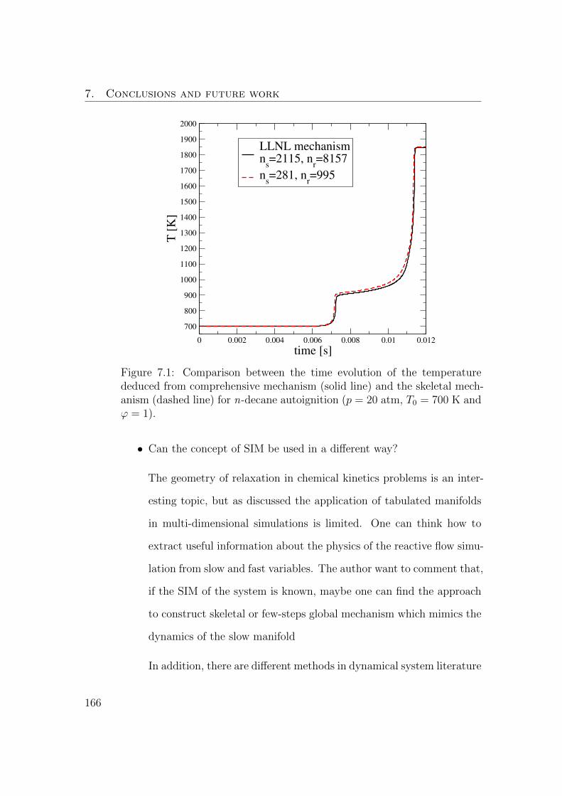
7. Conclusions and future work
0 0.002 0.004 0.006 0.008 0.01 0.012
time [s]
700
800
900
1000
1100
1200
1300
1400
1500
1600
1700
1800
1900
2000
T [
K]
LLNL mechanismn
s=2115, n
r=8157
ns=281, n
r=995
Figure 7.1: Comparison between the time evolution of the temperaturededuced from comprehensive mechanism (solid line) and the skeletal mech-anism (dashed line) for n-decane autoignition (p = 20 atm, T0 = 700 K andϕ = 1).
• Can the concept of SIM be used in a different way?
The geometry of relaxation in chemical kinetics problems is an inter-
esting topic, but as discussed the application of tabulated manifolds
in multi-dimensional simulations is limited. One can think how to
extract useful information about the physics of the reactive flow simu-
lation from slow and fast variables. The author want to comment that,
if the SIM of the system is known, maybe one can find the approach
to construct skeletal or few-steps global mechanism which mimics the
dynamics of the slow manifold
In addition, there are different methods in dynamical system literature
166

7.2. Directions for future work
for constructing the SIM which can be introduced for the combustion
community.
• Direct Numerical Simulations using skeletal mechanisms
The stability of hydrocarbon laminar/turbulent premixed flames is
the subject of ongoing studies. The low-Mach number solver based
on the spectral element code NEK5000 [191] was used to study hydro-
dynamic and thermodiffusive instabilities of laminar planar premixed
hydrogen flames (e.g. [192, 193]). In order to study instabilities of
methane flames under laminar and turbulent conditions, the entropy
production analysis was performed on a database generated from the
laminar planar premixed methane-air flame for T0 = 300 K, p = 1
atm and ϕ = 0.9 . The detailed methane mechanism (excluding ni-
trogen chemistry) consists of ns = 35 species and nr = 217 reactions
(D35) [5]. The skeletal mechanism (R20) includes ns = 20 species
and nr = 98 reactions, and the laminar flame speed SL and flame
thickness δf errors compared to the detailed one are less than 2% (see
table 7.1).
Table 7.1: methane/air premixed flame simulation
Mechanism SL (cm/s) δf (cm)D35 33.472 0.046539R20 33.114 0.047524
The temperature and selected species profiles deduced from the D35
and R20 mechanisms are compared in the Fig. 7.2, showing very good
agreement.
167
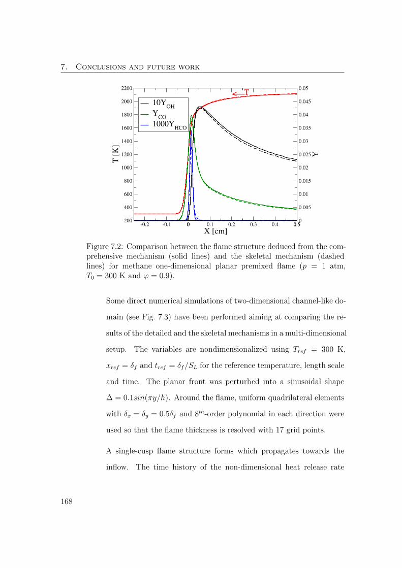
7. Conclusions and future work
0 0.5200
400
600
800
1000
1200
1400
1600
1800
2000
2200
T [
K]
-0.2 -0.1 0 0.1 0.2 0.3 0.4 0.5
X [cm]
0
0.005
0.01
0.015
0.02
0.025
0.03
0.035
0.04
0.045
0.05
Y
10YOH
YCO
1000YHCO
T
Figure 7.2: Comparison between the flame structure deduced from the com-prehensive mechanism (solid lines) and the skeletal mechanism (dashedlines) for methane one-dimensional planar premixed flame (p = 1 atm,T0 = 300 K and ϕ = 0.9).
Some direct numerical simulations of two-dimensional channel-like do-
main (see Fig. 7.3) have been performed aiming at comparing the re-
sults of the detailed and the skeletal mechanisms in a multi-dimensional
setup. The variables are nondimensionalized using Tref = 300 K,
xref = δf and tref = δf/SL for the reference temperature, length scale
and time. The planar front was perturbed into a sinusoidal shape
∆ = 0.1sin(πy/h). Around the flame, uniform quadrilateral elements
with δx = δy = 0.5δf and 8th-order polynomial in each direction were
used so that the flame thickness is resolved with 17 grid points.
A single-cusp flame structure forms which propagates towards the
inflow. The time history of the non-dimensional heat release rate
168

7.2. Directions for future work
Figure 7.3: Schematic of two-dimensional planar premixed flame setup andboundary conditions
0 10 20 30 40 50
t
110
115
120
125
130
135
140
145
150
HR
R
D35R20
Figure 7.4: Temporal evolution of the heat release rate (HRR) for detailed(D35) and the skeletal mechanism (R20)
(HRR) (Fig. 7.4) and isocontours of the temperature for different
times (Fig. 7.5), computed using the detailed and skeletal mechanisms
are compared, showing very good agreement. The computational time
169

7. Conclusions and future work
using the skeletal mechanism is three times lower, enabling parametric
studies and extension to three-dimensional turbulent conditions.
170

7.2. Directions for future work
(a)
(b)
(c)
(d)
Figure 7.5: Temperature isocontours of the methane-air flame propagatingin the 2D domain at (a) t = 12, (b) t = 15, (c) t = 20, and (d) t = 30. Upperand lower rows are deduced from the detailed and the skeletal mechanismrespectively.
171


Appendix A
Code segment for the entropy
production analysis
A database ‘samples.dat’ is generated by the constant enthalpy and pres-
sure batch reactor solution, using the detailed mechanism initial conditions
covering the range of interest. Pressure, p, temperature, T and mass frac-
tion of all species Y , are stored row-wise in the file ‘sample.dat’. KK and
II are the number of species and reactions, respectively, and ICWRK and
RCWRK the integer and real CHEMKIN work arrays. The stoichiometric
matrix is stored in NUKI, forward and reverse reaction rates in the FWDK
and REVK arrays, while the relative contribution of reactions to the total
entropy production DSDT is stored in DSDTK. If its contribution is larger
than the threshold, CUTOFF, the reaction is flagged in the array REINDX.
Species participating in important reactions are flagged in array SPINDX.
A slightly modified version of MECHMOD 3.42 [133] was used to gener-
ate the skeletal mechanisms by eliminating unimportant species from the
detailed scheme.
173

A. Code segment for the entropy production analysis
1 OPEN(unit=10,file=’samples.dat’,form=’formatted’)
2 100 CONTINUE
3 READ (UNIT=10, FMT=* ,END=200)P,T,(Y(K),K=1,KK)
4 CALL CKYTX(Y,ICKWRK,RCKWRK,X)
5 CALL CKKFKR (P,T,X,ICKWRK,RCKWRK,FWDK,REVK)
6 DO K = 1,II
7 DSDTK(K) = 0.0d0
8 ENDDO
9 DSDT = 0.d0
10 DO K = 1,II
11 IF (FWDK(K).LE.0.0d0) FWDK(K) = 1.0D-50
12 IF (REVK(K).LE.0.0d0) REVK(K) = 1.0D-50
13 DSDTK(K) = RU*(FWDK(K)-REVK(K))*(log((FWDK(K)/REVK(K))))
14 DSDT = DSDT + DSDTK(K)
15 ENDDO
16 DO K=1,II
17 IF ((DSDTK(K)/DSDT).gt.CUTOFF) ENT_IDX(K)=1
18 ENDDO
19 GO TO 100
20 200 CONTINUE
21 J = 0
22 DO K = 1, II
23 IF (ENT_IDX(K).eq.1) THEN
24 J = J + 1
25 REINDX(J)=K
174

26 ENDIF
27 ENDDO
28 CALL CKNU(KK, ICKWRK, RCKWRK, NUKI)
29 DO I = 1,KK
30 SPINDX(I)=0
31 ENDDO
32
33 DO K = 1, SIZEINDX
34 J = REINDX(K)
35 DO I =1, KK
36 IF (NUKI(I,J).ne.0) THEN
37 SPINDX(I)=1
38 ENDIF
39 ENDDO
40 ENDDO
175


Bibliography
[1] U. E. I. Administration, “Annual Energy Outlook 2014,” DOE/EIA,vol. 0383, pp. 1–269, 2014.
[2] F. Williams, Combustion theory: the fundamental theory of chemicallyreacting flow systems, vol. 54. Perseus Books, 1985.
[3] Z. Qin, V. V. Lissianski, H. Yang, W. C. Gardiner, S. G. Davis, andH. Wang,“Combustion chemistry of propane: A case study of detailedreaction mechanism optimization,”Proc. Combust. Inst., vol. 28, no. 2,pp. 1663–1669, 2000.
[4] H. J. Curran, P. Gaffuri, W. J. Pitz, and C. K. Westbrook, “A com-prehensive modeling study of n-heptane oxidation,” Combust. Flame,vol. 114, no. 1-2, pp. 149–177, 1998.
[5] G. P. Smith, D. M. Golden, M. Frenklach, N. W. Moriarty, B. Eiteneer,D. M. Golden, C. T. Bowman, R. K. Hanson, S. Song, W. C. Gardiner,V. V. Lissianski, and Z. Qin, “GRI-Mech 3.0.”
[6] P. Gokulakrishnan, C. C. Fuller, M. S. Klassen, R. G. Joklik, Y. N.Kochar, S. N. Vaden, T. C. Lieuwen, and J. M. Seitzman, “Experi-ments and modeling of propane combustion with vitiation,” Combust.Flame, vol. 161, no. 8, pp. 2038–2053, 2014.
[7] C. K. Westbrook, W. J. Pitz, O. Herbinet, H. J. Curran, and E. J.Silke, “A comprehensive detailed chemical kinetic reaction mecha-nism for combustion of n-alkane hydrocarbons from n-octane to n-hexadecane,” Combust. Flame, vol. 156, no. 1, pp. 181–199, 2009.
177

Bibliography
[8] S. M. Sarathy, C. K. Westbrook, M. Mehl, W. J. Pitz, C. Togbe,P. Dagaut, H. Wang, M. a. Oehlschlaeger, U. Niemann, K. Seshadri,P. S. Veloo, C. Ji, F. N. Egolfopoulos, and T. Lu, “Comprehensivechemical kinetic modeling of the oxidation of 2-methylalkanes fromC7 to C20,” Combust. Flame, vol. 158, no. 12, pp. 2338–2357, 2011.
[9] D. A. Goussis and U. Maas, “Model reduction for combustion chem-istry,” in Fluid Mech. its Appl., vol. 95, pp. 193–220, Springer, 2011.
[10] C. W. Gear, “Simultaneous Numerical Solution of Differential-Algebraic Equations,” IEEE Trans. Circuit Theory, vol. 18, no. 1,1971.
[11] L. Brugnano, F. Mazzia, and D. Trigiante, “Fifty years of stiffness,”Recent Adv. Comput. Appl. Math., pp. 1–21, 2011.
[12] B. Bhattacharjee, D. A. Schwer, P. I. Barton, and W. H. Green,“Optimally-reduced kinetic models: Reaction elimination in large-scale kinetic mechanisms,” Combust. Flame, vol. 135, no. 3, pp. 191–208, 2003.
[13] A. N. Gorban and I. V. Karlin, “Method of invariant manifold forchemical kinetics,” Chem. Eng. Sci., vol. 58, no. 21, pp. 4751–4768,2003.
[14] N. Peters, “Reducing mechanisms,” in Reduc. Kinet. Mech. Asymptot.Approx. Methane-Air Flames, pp. 48–67, Springer, 1991.
[15] T. Turanyi and A. S. Tomlin, Analysis of Kinetic Reaction Mecha-nisms. Berlin, Heidelberg: Springer Berlin Heidelberg, 2014.
[16] M. R. Roussel and S. J. Fraser, “On the geometry of transient relax-ation,” J. Chem. Phys., vol. 94, no. 11, pp. 7106–7113, 1991.
[17] J. Li, Z. Zhao, A. Kazakov, and F. L. Dryer, “An updated compre-hensive kinetic model of hydrogen combustion,” Int. J. Chem. Kinet.,vol. 36, no. 10, pp. 566–575, 2004.
[18] S. B. Pope, “Small scales, many species and the manifold challenges ofturbulent combustion,” Proc. Combust. Inst., vol. 34, no. 1, pp. 1–31,2013.
178

Bibliography
[19] M. Frenklach, K. Kailasanath, and E. S. Oran, “Systematic develop-ment of reduced reaction mechanisms for dynamic modeling,” Prog.Astronaut. Aeronaut., vol. 105, no. 2, pp. 365–376, 1986.
[20] T. Turanyi, “Sensitivity analysis of complex kinetic systems. Toolsand applications,” J. Math. Chem., vol. 5, no. 3, pp. 203–248, 1990.
[21] A. S. Tomlin, M. J. Pilling, T. Turanyi, J. H. Merkin, and J. Brind-ley, “Mechanism reduction for the oscillatory oxidation of hydrogen:Sensitivity and quasi-steady-state analyses,” Combust. Flame, vol. 91,no. 2, pp. 107–130, 1992.
[22] S. Vajda, P. Valko, and T. Turanyi, “Principal component analysis ofkinetic models,” Int. J. Chem. Kinet., vol. 17, no. 1, pp. 55–81, 1985.
[23] N. J. Brown, G. Li, and M. L. Koszykowski, “Mechanism reductionvia principal component analysis,” Int. J. Chem. Kinet., vol. 29, no. 6,pp. 393–414, 1997.
[24] C. E. Frouzakis and K. Boulouchos, “Analysis and Reduction of theCH4-Air Mechanism at Lean Conditions,” Combust. Sci. Technol.,vol. 159, no. 1, pp. 281–303, 2000.
[25] J. Warnatz, “The structure of laminar alkane-, alkene-, and acetyleneflames,” Symp. Combust., vol. 18, no. 1, pp. 369–384, 1981.
[26] J. Revel, J. C. Boettner, M. Cathonnet, and J. S. Bachman, “Deriva-tion of a global chemical kinetic mechanism for methane ignition andcombustion,” J. Chim. Phys., vol. 91, no. 4, pp. 365–382, 1994.
[27] T. Lu and C. K. Law, “A directed relation graph method for mecha-nism reduction,” Proc. Combust. Inst., vol. 30 I, no. 1, pp. 1333–1341,2005.
[28] W. Sun, Z. Chen, X. Gou, and Y. Ju, “A path flux analysis methodfor the reduction of detailed chemical kinetic mechanisms,” Combust.Flame, vol. 157, no. 7, pp. 1298–1307, 2010.
[29] T. Turanyi, “Reduction of large reaction mechanisms,” New J. Chem.,vol. 14, no. 11, pp. 795–803, 1990.
[30] H. Karadeniz, H. S. Soyhan, and C. Sorusbay, “Reduction of largekinetic mechanisms with a new approach to the necessity analysismethod,” Combust. Flame, vol. 159, no. 4, pp. 1467–1480, 2012.
179

Bibliography
[31] L. Petzold and W. Zhu, “Model reduction for chemical kinetics: Anoptimization approach,” AIChE J., vol. 45, no. 4, pp. 869–886, 1999.
[32] I. P. Androulakis, “Kinetic mechanism reduction based on an integerprogramming approach,” AIChE J., vol. 46, no. 2, pp. 361–371, 2000.
[33] M. Valorani, F. Creta, D. A. Goussis, J. C. Lee, and H. N. Najm, “Anautomatic procedure for the simplification of chemical kinetic mecha-nisms based on CSP,” Combust. Flame, vol. 146, no. 1-2, pp. 29–51,2006.
[34] D. A. Goussis and G. Skevis, “Nitrogen chemistry controlling stepsin methane-air premixed flames,” Comput. Fluid Solid Mech., vol. 1,pp. 650–653, 2005.
[35] N. Berglund and B. Gentz, “Noise-Induced Phenomena in Slow-FastDynamical Systems,” in Noise-Induced Phenom. Slow-Fast Dyn. Syst.,Probability and Its Applications, pp. 17–49, London: Springer-Verlag,2006.
[36] C. Kuehn, “A mathematical framework for critical transitions: Bifur-cations, fastslow systems and stochastic dynamics,” Phys. D Nonlin-ear Phenom., vol. 240, no. 12, pp. 1020–1035, 2011.
[37] M. Bodenstein and S. C. Lind, “Geschwindigkeit der Bildung desBromwasserstoffs aus seinen Elementen,”Zeitschrift fur Phys. Chemie,vol. 57, pp. 168–192, 1906.
[38] A. N. Al-Khateeb, J. M. Powers, S. Paolucci, A. J. Sommese, J. A.Diller, J. D. Hauenstein, and J. D. Mengers, “One-dimensional slowinvariant manifolds for spatially homogenous reactive systems,” J.Chem. Phys., vol. 131, no. 2, p. 024118, 2009.
[39] S. H. Lam and D. A. Goussis, “The CSP method for simplifying ki-netics,” Int. J. Chem. Kinet., vol. 26, no. 4, pp. 461–486, 1994.
[40] A. Zagaris, H. G. Kaper, and T. J. Kaper, “Fast and Slow Dynam-ics for the Computational Singular Perturbation Method,” MultiscaleModel. Simul., vol. 2, no. 4, pp. 613–638, 2004.
[41] E. Chiavazzo, A. N. Gorban, and I. V. Karlin, “Comparison of In-variant Manifolds for Model Reduction in Chemical Kinetics 1 Intro-duction 2 Theoretical background,” Commun. Comput. Phys., vol. 2,no. 5, pp. 964–992, 2007.
180

Bibliography
[42] U. Maas and S. Pope, “Simplifying chemical kinetics: Intrinsic low-dimensional manifolds in composition space,”Combust. Flame, vol. 88,no. 3-4, pp. 239–264, 1992.
[43] H. G. Kaper and T. J. Kaper, “Asymptotic analysis of two reduc-tion methods for systems of chemical reactions,” Phys. D NonlinearPhenom., vol. 165, no. 1-2, pp. 66–93, 2002.
[44] J. C. Keck and D. Gillespie, “Rate-controlled partial-equilibriummethod for treating reacting gas mixtures,” Combust. Flame, vol. 17,no. 2, pp. 237–241, 1971.
[45] J. C. Keck, “Rate-controlled constrained-equilibrium theory of chemi-cal reactions in complex systems,” Prog. Energy Combust. Sci., vol. 16,no. 2, pp. 125–154, 1990.
[46] Z. Ren, S. B. Pope, A. Vladimirsky, and J. M. Guckenheimer, “Theinvariant constrained equilibrium edge preimage curve method for thedimension reduction of chemical kinetics,” J. Chem. Phys., vol. 124,no. 11, p. 114111, 2006.
[47] D. Lebiedz, “Computing minimal entropy production trajectories: Anapproach to model reduction in chemical kinetics,” J. Chem. Phys.,vol. 120, no. 15, pp. 6890–6897, 2004.
[48] C. W. Gear, T. J. Kaper, I. G. Kevrekidis, and A. Zagaris, “Projectingto a Slow Manifold: Singularly Perturbed Systems and Legacy Codes,”SIAM J. Appl. Dyn. Syst., vol. 4, no. 3, p. 21, 2004.
[49] I. G. Kevrekidis and G. Samaey, “Equation-free multiscale computa-tion: algorithms and applications.,” Annu. Rev. Phys. Chem., vol. 60,pp. 321–344, 2009.
[50] D. Hilbert, “Mathematical problems,” Bull. Am. Math. Soc., vol. 8,no. 10, pp. 437–480, 1902.
[51] L. Saint-Raymond, Hydrodynamic Limits of the Boltzmann Equa-tion, vol. 1971 of Lecture Notes in Mathematics. Berlin, Heidelberg:Springer Berlin Heidelberg, 2009.
[52] M. Slemrod, “From Boltzmann to Euler: Hilbert’s 6th problem re-visited,” Comput. Math. with Appl., vol. 65, no. 10, pp. 1497–1501,2013.
181

Bibliography
[53] A. N. Gorban and I. V. Karlin, “Hilbert’s 6th problem: Exact and ap-proximate hydrodynamic manifolds for kinetic equations,” Bull. Am.Math. Soc., vol. 51, no. 2, pp. 187–246, 2014.
[54] S. Chapman and T. G. Cowling, The mathematical theory of non-uniform gases: an account of the kinetic theory of viscosity, thermalconduction and diffusion in gases. 1970.
[55] H. Grad, “On the kinetic theory of rarefied gases,” Commun. PureAppl. Math., vol. 2, no. 4, pp. 331–407, 1949.
[56] I. V. Karlin and A. N. Gorban, “Hydrodynamics from Grad’s equa-tions: What can we learn from exact solutions?,” Ann. Phys., vol. 11,no. 10-11, pp. 783–833, 2002.
[57] A. N. Gorban, I. V. Karlin, and A. Y. Zinovyev, “Invariant grids forreaction kinetics,” Phys. A Stat. Mech. its Appl., vol. 333, no. 1-4,pp. 106–154, 2004.
[58] E. Chiavazzo and I. V. Karlin, “Adaptive simplification of complexmultiscale systems,”Phys. Rev. E - Stat. Nonlinear, Soft Matter Phys.,vol. 83, no. 3, p. 036706, 2011.
[59] A. N. Gorban and I. V. Karlin, Invariant manifolds for physical andchemical kinetics. Springer, 2009.
[60] A. Debussche and R. Temam,“Inertial Manifolds and Slow Manifolds,”Appl. Math. Lett., vol. 4, no. 4, pp. 73–76, 1991.
[61] J. C. Robinson, “A concise proof of the “geometric” construction ofinertial manifolds,” Phys. Lett. A, vol. 200, no. 6, pp. 415–417, 1995.
[62] A. N. Gorban and I. V. Karlin, “Thermodynamic parameterization,”Phys. A Stat. Mech. its Appl., vol. 190, no. 3-4, pp. 393–404, 1992.
[63] A. C. Tsoumanis, K. Rajendran, C. I. Siettos, and I. G. Kevrekidis,“Coarse-graining the dynamics of network evolution: The rise and fallof a networked society,” AIP Conf. Proc., vol. 1389, no. 8, pp. 42–45,2011.
[64] V. Bykov, I. Goldfarb, V. Gol’dshtein, and U. Maas, “On a modifiedversion of ILDM approach: Asymptotic analysis based on integralmanifolds,” IMA J. Appl. Math., vol. 71, no. 3, pp. 359–382, 2006.
182

Bibliography
[65] S. B. Pope,“Gibbs function continuation for the stable computation ofchemical equilibrium,” Combust. Flame, vol. 139, no. 3, pp. 222–226,2004.
[66] V. Bykov and U. Maas,“Extension of the ILDM method to the domainof slow chemistry,” Proc. Combust. Inst., vol. 31 I, no. 1, pp. 465–472,2007.
[67] Q. Tang and S. B. Pope, “A more accurate projection in the rate-controlled constrained-equilibrium method for dimension reductionof combustion chemistry,” Combust. Theory Model., vol. 8, no. 2,pp. 255–279, 2004.
[68] W. P. Jones and S. Rigopoulos, “Rate-controlled constrained equilib-rium: Formulation and application to nonpremixed laminar flames,”Combust. Flame, vol. 142, no. 3, pp. 223–234, 2005.
[69] S. Rigopoulos and T. Lø vas, “A LOI-RCCE methodology for reducingchemical kinetics, with application to laminar premixed flames,” Proc.Combust. Inst., vol. 32 I, no. 1, pp. 569–576, 2009.
[70] R. Law, M. Metghalchi, and J. C. Keck, “Rate-controlled constrainedequilibrium calculation of ignition delay times in hydrogen-oxygenmixtures,” Symp. Combust., vol. 22, no. 1, pp. 1705–1713, 1989.
[71] G. Beretta, J. C. Keck, M. Janbozorgi, and H. Metghalchi, “The rate-controlled constrained-equilibrium approach to far from local equilib-rium thermodynamics,” Entropy, vol. 14, no. 2, pp. 92–130, 2012.
[72] P. S. Bishnu, D. Hamiroune, M. Metghalchi, and J. C. Keck,“Constrained-equilibrium calculations for chemical systems subject togeneralized linear constraints using the NASA and STANJAN equilib-rium programs,” Combust. Theory Model., vol. 1, no. 3, pp. 295–312,1997.
[73] D. Hamiroune, P. Bishnu, M. Metghalchi, and J. C. Keck, “Rate-controlled constrained-equilibrium method using constraint poten-tials,” Combust. Theory Model., vol. 2, no. 1, pp. 81–94, 1998.
[74] M. Janbozorgi, S. Ugarte, H. Metghalchi, and J. C. Keck, “Com-bustion modeling of mono-carbon fuels using the rate-controlledconstrained-equilibrium method,” Combust. Flame, vol. 156, no. 10,pp. 1871–1885, 2009.
183
Bibliography
[75] V. Hiremath, S. R. Lantz, H. Wang, and S. B. Pope, “Large-scale par-allel simulations of turbulent combustion using combined dimensionreduction and tabulation of chemistry,” Proc. Combust. Inst., vol. 34,no. 1, pp. 205–215, 2013.
[76] O. Gicquel, D. Thevenin, M. Hilka, and N. Darabiha, “Direct nu-merical simulation of turbulent premixed flames using intrinsic low-dimensional manifolds,” Combust. Theory Model., vol. 3, no. 3,pp. 479–502, 1999.
[77] S. H. Lam and D. A. Coussis, “Understanding complex chemical ki-netics with computational singular perturbation,” Symp. Combust.,vol. 22, no. 1, pp. 931–941, 1989.
[78] A. N. Gorban and I. V. Karlin, “Uniqueness of thermodynamic projec-tor and kinetic basis of molecular individualism,” Phys. A Stat. Mech.its Appl., vol. 336, no. 3-4, pp. 391–432, 2004.
[79] E. Chiavazzo, I. V. Karlin, and A. N. Gorban, “The role of thermo-dynamics in model reduction when using invariant grids,” Commun.Comput. Phys., vol. 8, no. 4, pp. 701–734, 2010.
[80] D. Schmidt, J. Segatz, U. Riedel, J. Warnatz, and U. Maas, “Simula-tion of Laminar Methane-Air Flames using Automatically SimplifiedChemical Kinetics,” Combust. Sci. Technol., vol. 113, no. 1, pp. 3–16,1996.
[81] S. B. Pope, “The computation of constrained and unconstrained equi-librium compositions of ideal gas mixtures using Gibbs function con-tinuation,” tech. rep., Cornell University, 2003.
[82] S. B. Pope, “CEQ: A FORTRAN library to compute equilibrium com-positions using Gibbs function continuation,” 2003.
[83] W. I. Thacker, J. Zhang, L. Watson, J. B. Birch, M. A. Iyer, andM. W. Berry, “Algorithm 905,” ACM Trans. Math. Softw., vol. 37,no. 3, pp. 1–20, 2010.
[84] P. N. Brown, G. D. Byrne, and A. C. Hindmarsh, “VODE: A Variable-Coefficient ODE Solver,” SIAM J. Sci. Stat. Comput., vol. 10, no. 5,pp. 1038–1051, 1989.
184

Bibliography
[85] M. R. Roussel and S. J. Fraser, “Global analysis of enzyme inhibitionkinetics,” J. Phys. Chem., vol. 97, no. 31, pp. 8316–8327, 1993.
[86] W. P. Jones and S. Rigopoulos, “Reduced chemistry for hydrogenand methanol premixed flames via RCCE,” Combust. Theory Model.,vol. 11, no. 5, pp. 755–780, 2007.
[87] R. J. Kee, J. F. Grcar, M. D. Smooke, and J. A. Miller, “PREMIX:a Fortran program for modeling steady laminar one-dimensional pre-mixed flames,” tech. rep., 1985.
[88] R. L. G. M. Eggels and L. P. H. de Goey, “Mathematically reducedreaction mechanisms applied to adiabatic flat hydrogen/air flames,”Combust. Flame, vol. 100, no. 4, pp. 559–570, 1995.
[89] C. D. Levermore, “Moment closure hierarchies for kinetic theories,” J.Stat. Phys., vol. 83, pp. 1021–1065, June 1996.
[90] A. N. Gorban and I. V. Karlin, “Quasi-equilibrium closure hierarchiesfor the Boltzmann equation,” Phys. A Stat. Mech. its Appl., vol. 360,no. 2, pp. 325–364, 2006.
[91] I. V. Karlin, S. S. Chikatamarla, and M. Kooshkbaghi, “Non-perturbative hydrodynamic limits: A case study,” Phys. A Stat. Mech.its Appl., vol. 403, pp. 189–194, 2014.
[92] M. Kooshkbaghi, C. E. Frouzakis, E. Chiavazzo, K. Boulouchos, andI. V. Karlin, “The global relaxation redistribution method for reduc-tion of combustion kinetics,”J. Chem. Phys., vol. 141, no. 4, p. 044102,2014.
[93] E. Chiavazzo, I. V. Karlin, C. E. Frouzakis, and K. Boulouchos,“Method of invariant grid for model reduction of hydrogen combus-tion,” Proc. Combust. Inst., vol. 32, no. 1, pp. 519–526, 2009.
[94] A. N. Kolmogorov, “New Metric Invariant of Transitive DynamicalSystems and Endomorphisms of Lebesgue Spaces,” Dokl. Russ. Acad.Sci., vol. 119, no. N5, pp. 861–864, 1958.
[95] Y. G. Sinai, “On the Notion of Entropy of a Dynamical System,” Dokl.Russ. Acad. Sci., vol. 124, pp. 768–771, 1959.
[96] P. Ball, “Chaos-theory pioneer nabs Abel Prize,” Nature, 2014.
185

Bibliography
[97] J. Keener and S. James, Mathematical Physiology, vol. 8 of Interdis-ciplinary Applied Mathematics. New York: Springer-Verlag, 1998.
[98] A. H. Nguyen and S. J. Fraser, “Geometrical picture of reaction inenzyme kinetics,” J. Chem. Phys., vol. 91, no. 1, p. 186, 1989.
[99] M. R. Roussel and T. Tang, “The functional equation truncationmethod for approximating slow invariant manifolds: a rapid methodfor computing intrinsic low-dimensional manifolds.,” J. Chem. Phys.,vol. 125, no. 21, p. 214103, 2006.
[100] A. N. Gorban and M. Shahzad, “The Michaelis-Menten-StueckelbergTheorem,” Entropy, vol. 13, no. 12, pp. 966–1019, 2011.
[101] J. Eckmann and D. Ruelle, “Ergodic theory of chaos and strange at-tractors,” Rev. Mod. Phys., vol. 57, no. 3, pp. 617–656, 1985.
[102] A. Wolf, J. Swift, H. Swinney, and J. Vastano,“Determining Lyapunovexponents from a time series,” Phys. D Nonlinear Phenom., vol. 16,no. 3, pp. 285–317, 1985.
[103] K. D. Mease, S. Bharadwaj, and S. Iravanchy, “Timescale analysis fornonlinear dynamical systems,” J. Guid. Control. Dyn., vol. 26, no. 2,pp. 318–330, 2003.
[104] R. J. Kee, G. Dixon-Lewis, J. Warnatz, M. E. Coltrin, and J. A. Miller,“Chemkin-III: a Fortran chemical kinetics package for the analysis ofgas-phase chemical and plasma kinetics,” tech. rep., Sandia NationalLaboratories, 1996.
[105] P. S. Gregory, D. M. Golden, M. Frenklach, N. W. Moriarty, B. Eite-neer, M. Goldenberg, C. T. Bowman, R. K. Hanson, S. Song, W. C.Gardiner, V. V. Lissianski, and Z. Qin, “GRI-Mech 1.2,” 1994.
[106] L. Tosatto, B. A. V. Bennett, and M. D. Smooke, “Comparison ofdifferent DRG-based methods for the skeletal reduction of JP-8 sur-rogate mechanisms,” Combust. Flame, vol. 160, no. 9, pp. 1572–1582,2013.
[107] M. Kooshkbaghi, C. E. Frouzakis, K. Boulouchos, and I. V. Kar-lin, “Entropy production analysis for mechanism reduction,” Combust.Flame, vol. 161, no. 6, pp. 1507–1515, 2014.
186

Bibliography
[108] D. A. Schwer, P. Lu, and W. H. Green, “An adaptive chemistryapproach to modeling complex kinetics in reacting flows,” Combust.Flame, vol. 133, no. 4, pp. 451–465, 2003.
[109] K. He, M. G. Ierapetritou, and I. P. Androulakis, “A graph-basedapproach to developing adaptive representations of complex reactionmechanisms,” Combust. Flame, vol. 155, no. 4, pp. 585–604, 2008.
[110] A. Massias, D. Diamantis, E. Mastorakos, and D. A. Goussis, “Analgorithm for the construction of global reduced mechanisms withCSP data,” Combust. Flame, vol. 117, no. 4, pp. 685–708, 1999.
[111] I. Banerjee and M. Ieapetritou, “An adaptive reduction scheme tomodel reactive flow,” Combust. Flame, vol. 144, no. 3, pp. 619–633,2006.
[112] T. Lu, Y. Ju, and C. K. Law, “Complex CSP for chemistry reductionand analysis,” Combust. Flame, vol. 126, no. 1-2, pp. 1445–1455, 2001.
[113] T. Lu and C. K. Law, “A criterion based on computational singularperturbation for the identification of quasi steady state species: Areduced mechanism for methane oxidation with NO chemistry,” Com-bust. Flame, vol. 154, no. 4, pp. 761–774, 2008.
[114] M. Valorani, F. Creta, F. Donato, H. N. Najm, and D. A. Goussis,“Skeletal mechanism generation and analysis for n-heptane with CSP,”Proc. Combust. Inst., vol. 31, no. 1, pp. 483–490, 2007.
[115] T. Lu and C. K. Law, “On the applicability of directed relation graphsto the reduction of reaction mechanisms,” Combust. Flame, vol. 146,no. 3, pp. 472–483, 2006.
[116] T. Lu and C. K. Law, “Linear time reduction of large kinetic mecha-nisms with directed relation graph: n-heptane and iso-octane,” Com-bust. Flame, vol. 144, no. 1-2, pp. 24–36, 2006.
[117] T. Lu and C. Law,“Strategies for mechanism reduction for large hydro-carbons: n-heptane,” Combust. Flame, vol. 154, no. 1-2, pp. 153–163,2008.
[118] Z. Luo, T. Lu, and J. Liu, “A reduced mechanism for ethy-lene/methane mixtures with excessive NO enrichment,” Combust.Flame, vol. 158, no. 7, pp. 1245–1254, 2011.
187

Bibliography
[119] P. Pepiotdesjardins and H. Pitsch, “An efficient error-propagation-based reduction method for large chemical kinetic mechanisms,” Com-bust. Flame, vol. 154, no. 1-2, pp. 67–81, 2008.
[120] K. E. Niemeyer and C.-J. Sung, “On the importance of graph searchalgorithms for DRGEP-based mechanism reduction methods,” Com-bust. Flame, vol. 158, no. 8, pp. 1439–1443, 2011.
[121] X. Zheng, T. Lu, and C. Law, “Experimental counterflow ignition tem-peratures and reaction mechanisms of 1,3-butadiene,” Proc. Combust.Inst., vol. 31, no. 1, pp. 367–375, 2007.
[122] K. E. Niemeyer, C.-J. Sung, and M. P. Raju, “Skeletal mechanismgeneration for surrogate fuels using directed relation graph with errorpropagation and sensitivity analysis,” Combust. Flame, vol. 157, no. 9,pp. 1760–1770, 2010.
[123] L. Tosatto, B. Bennett, and M. Smooke, “A transport-flux-based di-rected relation graph method for the spatially inhomogeneous instan-taneous reduction of chemical kinetic mechanisms,” Combust. Flame,vol. 158, pp. 820–835, May 2011.
[124] G. Li and H. Rabitz, “A general analysis of approximate lumping inchemical kinetics,” Chem. Eng. Sci., vol. 45, no. 4, pp. 977–1002, 1990.
[125] H. Huang, M. Fairweather, J. F. Griffiths, A. S. Tomlin, and R. B.Brad, “A systematic lumping approach for the reduction of compre-hensive kinetic models,” Proc. Combust. Inst., vol. 30, no. 1, pp. 1309–1316, 2005.
[126] T. Lu and C. K. Law, “Diffusion coefficient reduction through speciesbundling,” Combust. Flame, vol. 148, no. 3, pp. 117–126, 2007.
[127] L. Liang, J. G. Stevens, and J. T. Farrell, “A dynamic adaptive chem-istry scheme for reactive flow computations,” Proc. Combust. Inst.,vol. 32, no. 1, pp. 527–534, 2009.
[128] L. Liang, J. G. Stevens, S. Raman, and J. T. Farrell, “The use ofdynamic adaptive chemistry in combustion simulation of gasoline sur-rogate fuels,” Combust. Flame, vol. 156, no. 7, pp. 1493–1502, 2009.
[129] F. Contino, H. Jeanmart, T. Lucchini, and G. D’Errico, “Couplingof in situ adaptive tabulation and dynamic adaptive chemistry: An
188

Bibliography
effective method for solving combustion in engine simulations,” Proc.Combust. Inst., vol. 33, no. 2, pp. 3057–3064, 2011.
[130] I. Prigogine and P. V. Rysselberghe, Introduction to Thermodynamicsof Irreversible Processes, vol. 110. 1963.
[131] T. Donder and P. V. Rysselberghe, Thermodynamic theory of affinity,Band 1. 1936.
[132] D. Kondepudi and I. Prigogine, Modern Thermodynamics: From HeatEngines to Dissipative Structures. Wiley, 1 ed., 1998.
[133] “MECHMOD: Manipulation of CHEMKIN format mechanisms.”http://garfield.chem.elte.hu/Combustion/mechmod.htm/,2003.
[134] A. N. Gorban, E. M. Mirkes, and G. S. Yablonsky, “Thermodynamicsin the limit of irreversible reactions,” Phys. A Stat. Mech. its Appl.,vol. 392, no. 6, pp. 1318–1335, 2013.
[135] N. Peters, G. Paczko, R. Seiser, and K. Seshadri, “Temperature cross-over and non-thermal runaway at two-stage ignition of n-heptane,”Combust. Flame, vol. 128, no. 1-2, pp. 38–59, 2002.
[136] “n-heptane, Detailed Mechanism, Version 2.”https://www-pls.llnl.gov/?url=science_and_
technology-chemistry-combustion-nc7h16, 1998.
[137] J. Prager, H. N. Najm, M. Valorani, and D. A. Goussis,“Skeletal mech-anism generation with CSP and validation for premixed n-heptaneflames,” Proc. Combust. Inst., vol. 32, no. 1, pp. 509–517, 2009.
[138] J. B. Heywood, Internal Combustion Engine Fundamentals, vol. 21.1988.
[139] K. Nishida, T. Takagi, and S. Kinoshita, “Analysis of entropy genera-tion and exergy loss during combustion,” Proc. Combust. Inst., vol. 29,no. 1, pp. 869–874, 2002.
[140] O. Herbinet and G. Dayma, “Jet-Stirred Reactors,” Clean. Combust.,2013.
[141] O. Bilous and N. R. Amundson, “Chemical reactor stability and sen-sitivity,” AIChE J., vol. 1, no. 4, pp. 513–521, 1955.
189

Bibliography
[142] R. Aris and N. R. Amundson, “An analysis of chemical reactor stabil-ity and control-I,” Chem. Eng. Sci., vol. 7, no. 3, pp. 121–131, 1958.
[143] A. Uppal, W. Ray, and A. Poore,“On the dynamic behavior of continu-ous stirred tank reactors,” Chem. Eng. Sci., vol. 29, no. 4, pp. 967–985,1974.
[144] W. W. Farr and R. Aris, ““Yet who would have thought the old manto have had so much blood in him?”—Reflections on the multiplicityof steady states of the stirred tank reactor,” Chem. Eng. Sci., vol. 41,no. 6, pp. 1385–1402, 1986.
[145] P. Gray and S. K. Scott, Chemical Oscillations and Instabilities.Springer, 1996.
[146] C. K. Law, Combustion Physics. Cambridge University Press, 2006.
[147] A. B. Poore, “A model equation arising from chemical reactor theory,”Arch. Ration. Mech. Anal., vol. 52, no. 4, pp. 358–388, 1973.
[148] V. Balakotaiah and D. Luss, “Structure of the steady-state solutionsof lumped-parameter chemically reacting systems,” Chem. Eng. Sci.,vol. 37, no. 11, pp. 1611–1623, 1982.
[149] H. S. Sidhu, M. I. Nelson, G. N. Mercer, and R. O. Weber, “Dynamicalanalysis of an elementary X + Y = P reaction in a continuously stirredtank reactor,” J. Math. Chem., vol. 28, pp. 353–375, Dec. 2000.
[150] R. Warden, R. Aris, and N. Amundson, “An analysis of chemicalreactor stability and control—VIII,” Chem. Eng. Sci., vol. 19, no. 3,pp. 149–172, 1964.
[151] F. Strozzi and J. Zaldıvar,“A general method for assessing the thermalstability of batch chemical reactors by sensitivity calculation based onLyapunov exponents,” Chem. Eng. Sci., vol. 49, no. 16, pp. 2681–2688,1994.
[152] J. Alvarez, J. Alvarez, and E. Gonzalez, “Global nonlinear control ofa continuous stirred tank reactor,” Chem. Eng. Sci., vol. 44, no. 5,pp. 1147–1160, 1989.
[153] J. F. Griffiths and S. K. Scott, “Thermokinetic interactions: Funda-mentals of spontaneous ignition and cool flames,” Prog. Energy Com-bust. Sci., vol. 13, no. 3, pp. 161–197, 1987.
190
Bibliography
[154] S. Kalamatianos and D. G. Vlachos, “Bifurcation Behavior of Pre-mixed Hydrogen/Air Mixtures in a Continuous Stirred Tank Reactor,”Combust. Sci. Technol., vol. 109, no. 1-6, pp. 347–371, 1995.
[155] S. Kalamatianos, Y. K. Park, and D. G. Vlachos, “Two-parameter con-tinuation algorithms for sensitivity analysis, parametric dependence,reduced mechanisms, and stability criteria of ignition and extinction,”Combust. Flame, vol. 112, no. 1-2, pp. 45–61, 1998.
[156] R. J. Olsen and D. G. Vlachos, “A Complete Pressure TemperatureDiagram for Air Oxidation of Hydrogen in a Continuous Flow StirredTank Reactor,” J. Phys. Chem. A, vol. 103, no. 40, pp. 7990–7999,1999.
[157] R. Shan and T. Lu, “Ignition and extinction in perfectly stirred re-actors with detailed chemistry,” Combust. Flame, vol. 159, no. 6,pp. 2069–2076, 2012.
[158] R. Shan and T. Lu, “A bifurcation analysis for limit flame phenomenaof DME/air in perfectly stirred reactors,” Combust. Flame, vol. 161,no. 7, pp. 1716–1723, 2014.
[159] R. Shan, C. S. Yoo, J. H. Chen, and T. Lu, “Computational diag-nostics for n-heptane flames with chemical explosive mode analysis,”Combust. Flame, vol. 159, no. 10, pp. 3119–3127, 2012.
[160] T. Lu and C. K. Law, “Toward accommodating realistic fuel chem-istry in large-scale computations,”Prog. Energy Combust. Sci., vol. 35,no. 2, pp. 192–215, 2009.
[161] H. B. Keller, Lectures on numerical methods in bifurcation problems.Springer, 1987.
[162] E. J. Doedel, “AUTO: A program for the automatic bifurcation anal-ysis of autonomous systems,” Congr. Numer, 1981.
[163] E. J. Doedel and B. E. Oldeman, AUTO-07P : Continuation andBifurcation Software for Ordinary Differential Equations. ConcordiaUniversity, Montreal, Canada, 2009.
[164] A. Kazakov, M. Chaos, Z. Zhao, and F. L. Dryer, “Computationalsingular perturbation analysis of two-stage ignition of large hydrocar-bons.,” J. Phys. Chem. A, vol. 110, no. 21, pp. 7003–9, 2006.
191

Bibliography
[165] D. J. Diamantis, D. C. Kyritsis, and D. A. Goussis, “Two Stage Ig-nition of n-heptane: Identifying the Chemistry Setting the ExplosiveTime Scales,” in Second Int. Work. Model Reduct. React. Flows, 2009.
[166] S. Gupta, H. G. Im, and M. Valorani, “Analysis of n-heptane auto-ignition characteristics using computational singular perturbation,”Proc. Combust. Inst., vol. 34, no. 1, pp. 1125–1133, 2013.
[167] W. Liu, C. K. Law, and T. Lu,“Multiple criticality and staged ignitionof methane in the counterflow,” Int. J. Chem. Kinet., vol. 41, pp. 764–776, Dec. 2009.
[168] H. Meijer, F. Dercole, and B. Oldeman, “Numerical bifurcation anal-ysis,” Encycl. Complex. Syst. Sci., pp. 6329–6352, 2009.
[169] I. Kuznetsov, Elements of applied bifurcation theory. Springer, 1998.
[170] R. J. Olsen and I. R. Epstein, “Bifurcation analysis of chemical re-action mechanisms. I. Steady state bifurcation structure,” J. Chem.Phys., vol. 94, no. 4, p. 3083, 1991.
[171] D. J. Diamantis, E. Mastorakos, and D. A. Goussis, “H2/air autoigni-tion: The nature and interaction of the developing explosive modes,”Combust. Theory Model., pp. 1–52, 2015.
[172] M. Valorani, H. N. Najm, and D. A. Goussis, “CSP analysis of atransient flame-vortex interaction,” Combust. Flame, vol. 134, no. 1-2,pp. 35–53, 2003.
[173] T. Lu, C. S. Yoo, J. H. Chen, and C. K. Law, “Three-dimensionaldirect numerical simulation of a turbulent lifted hydrogen jet flame inheated coflow: a chemical explosive mode analysis,” J. Fluid Mech.,vol. 652, pp. 45–64, 2010.
[174] Z. Luo, C. S. Yoo, E. S. Richardson, J. H. Chen, C. K. Law, andT. Lu, “Chemical explosive mode analysis for a turbulent lifted ethy-lene jet flame in highly-heated coflow,” Combust. Flame, vol. 159,no. 1, pp. 265–274, 2012.
[175] D. A. Goussis and H. N. Najm, “Model Reduction and Physical Un-derstanding of Slowly Oscillating Processes: The Circadian Cycle,”Multiscale Model. Simul., vol. 5, no. 4, pp. 1297–1332, 2006.
192

Bibliography
[176] L. Hascoet and V. Pascual, “The Tapenade Automatic Differentiationtool: principles, model, and specification,” ACM Trans. Math. Softw.,vol. 20, 2013.
[177] E. Anderson, Z. Bai, C. Bischof, S. Blackford, J. Demmel, J. Don-garra, J. Du Croz, A. Greenbaum, S. Hammarling, A. McKenney,and D. Sorensen, LAPACK Users’ Guide. Philadelphia, PA: Societyfor Industrial and Applied Mathematics, third ed., 1999.
[178] R. Tolman and P. Fine, “On the Irreversible Production of Entropy,”Rev. Mod. Phys., vol. 20, no. 1, pp. 51–77, 1948.
[179] W. R. Dunbar and N. Lior, “Sources of combustion irreversibility,”Combust. Sci. Technol., 1994.
[180] I. Glassman and R. A. Yetter, Combustion. 2008.
[181] C. K. Westbrook, “Chemical kinetics of hydrocarbon ignition inpractical combustion systems,” Proc. Combust. Inst., vol. 28, no. 2,pp. 1563–1577, 2000.
[182] P. D. Kourdis and D. A. Goussis, “Glycolysis in Saccharomyces cere-visiae: algorithmic exploration of robustness and origin of oscilla-tions.,” Math. Biosci., vol. 243, no. 2, pp. 190–214, 2013.
[183] A. V. Bobylev, “The Chapman-Enskog and Grad methods for solvingthe Boltzmann equation,” Akad. Nauk SSSR Dokl., 1982.
[184] M. Slemrod, “Chapman-Enskog– viscosity-capillarity,” Q. Appl.Math., vol. 70, no. 3, pp. 613–624, 2012.
[185] F. J. Dyson,“The S Matrix in Quantum Electrodynamics,”Phys. Rev.,vol. 75, no. 11, pp. 1736–1755, 1949.
[186] J. Schwinger, “On the Green’s functions of quantized fields. I,” Proc.Natl. Acad. Sci., vol. 37, no. 7, pp. 452–455, 1951.
[187] S. Succi, H. Chen, and S. Orszag, “Relaxation approximations andkinetic models of fluid turbulence,” Phys. A Stat. Mech. its Appl.,vol. 362, no. 1, pp. 1–5, 2006.
[188] J. Latt, B. Chopard, S. Succi, and F. Toschi, “Numerical analysis ofthe averaged flow field in a turbulent lattice Boltzmann simulation,”Phys. A Stat. Mech. its Appl., vol. 362, no. 1, pp. 6–10, 2006.
193

Bibliography
[189] A. Singer, R. Erban, I. G. Kevrekidis, and R. R. Coifman, “Detectingintrinsic slow variables in stochastic dynamical systems by anisotropicdiffusion maps.,”Proc. Natl. Acad. Sci. U. S. A., vol. 106, pp. 16090–5,Sept. 2009.
[190] C. J. Dsilva, R. Talmon, N. Rabin, R. R. Coifman, and I. G.Kevrekidis, “Nonlinear intrinsic variables and state reconstruction inmultiscale simulations.,” J. Chem. Phys., vol. 139, p. 184109, Nov.2013.
[191] Fischer, P. F. and Lottes, J. W. and Kerkemier, S. G., “NEK5000.”http://nek5000.mcs.anl.gov., 2008.
[192] C. Altantzis, C. E. Frouzakis, A. G. Tomboulides, M. Matalon, andK. Boulouchos, “Hydrodynamic and thermodiffusive instability effectson the evolution of laminar planar lean premixed hydrogen flames,” J.Fluid Mech., vol. 700, pp. 329–361, May 2012.
[193] C. Altantzis, C. E. Frouzakis, A. G. Tomboulides, and K. Boulou-chos, “Numerical simulation of propagating circular and cylindricallean premixed hydrogen/air flames,” Proc. Combust. Inst., vol. 34,pp. 1109–1115, Jan. 2013.
194

LAVLaboratorium für Aerothermochemie und VerbrennungssystemeAerothermochemistry and Combustion Systems Laboratory
Address: ETH Zurich,Institut f. EnergietechnikML L 18, Sonneggstrasse 38092 Zurich
Phone: +41 (44) 632 26 50Website: www.lav.ethz.ch/people/mahdikwww.lav.ethz.ch/people/mahdik
E-mail: [email protected]@lav.mavt.ethz.ch
E-mail: [email protected]@gmail.com
Gender: MaleNationality: IranianMarital status: SingleBirth-date: 25-01-1986Place of Birth: Tehran
Curriculum VitæMahdi Kooshkbaghi
Education
2012 – 2015 • Ph.D in Mechanical Engineering at LAV, ETH Zurich2008 – 2011 • M.Sc. in Mechanical Engineering at Tehran Polytechnic2008 – 2010 • B.Sc. in Aerospace Engineering at Tehran Polytechnic2004 – 2008 • B.Sc. in Mechanical Engineering at Tehran Polytechnic
Journal Publications
2015 • Kooshkbaghi, Mahdi, Christos E. Frouzakis, Konstantinos Boulouchos, and Iliya V. Karlin.“n-Heptane/air combustion in perfectly stirred reactors: Dynamics, bifurcations and dominantreactions at critical conditions.” Combustion and Flame (2015), 162, no. 9 (2015): 3166-3179.
2014 • Kooshkbaghi, Mahdi, Christos E. Frouzakis, Konstantinos Boulouchos, and Iliya V. Karlin.“The global relaxation redistribution method for reduction of combustion kinetics.” Journal ofChemical Physics, 141, 044102.
• Kooshkbaghi, Mahdi, Christos E. Frouzakis, Konstantinos Boulouchos, and Ilya V. Karlin.“Entropy production analysis for mechanism reduction.” Combustion and Flame, 161, no. 6:1507-1515.
• Karlin, I. V., S. S. Chikatamarla, and M. Kooshkbaghi. “Non-perturbative hydrodynamiclimits: A case study.” Physica A: Statistical Mechanics and its Applications 403: 189-194.
2013 • Kooshkbaghi, Mahdi, and Bamdad Lessani. “A collocated grid, projection method fortimeaccurate calculation of lowMach number variable density flows in general curvilinearcoordinates.” International Journal for Numerical Methods in Fluids 72, no. 3: 301-319.
2010 • Shokouhmand, H., M. Fakoor Pakdaman, and M. Kooshkbaghi. “A similarity solution in orderto solve the governing equations of laminar separated fluids with a flat plate.” Communicationsin Nonlinear Science and Numerical Simulation 15, no. 12: 3965-3973.

Conference Proceedings
2014 • Kooshkbaghi, Mahdi, Christos E. Frouzakis, Eliodoro Chiavazzo, Ilya V. Karlin, and Kon-stantinos Boulouchos. “New Approaches For The Construction Of Reduced And SkeletalMechanisms”. IEA’s 36th Task Leaders Meeting, Stavanger, Norway.
2013 • Kooshkbaghi, Mahdi, Christos E. Frouzakis, Eliodoro Chiavazzo, Ilya V. Karlin, and Konstanti-nos Boulouchos. “Relaxation Redistribution Method for model reduction”. 4th IWMRRF,San Francisco, California, USA.
2009 • Rahimian, M.H, Fakoor Pakdaman, M. and Kooshkbaghi, M., “An Analytical and NumericalSimilarity Solution for Laminar Flow and Heat Transfer Between Two Separated Fluids”.,ISPT20, Vancouver, Canada.
Top Related