


Languages
Pages
Legal

On the Computational Complexity of Deep Learning
Shai Shalev-Shwartz
School of CS and Engineering,The Hebrew University of Jerusalem
”Optimization and Statistical Learning”,Les Houches, January 2014
Based on joint work with:Roi Livni and Ohad Shamir,Amit Daniely and Nati Linial,Tong Zhang
Shalev-Shwartz (HU) DL OSL’15 1 / 35

PAC Learning
Goal (informal): Learn an accurate mapping h : X → Y based onexamples ((x1, y1), . . . , (xn, yn)) ∈ (X × Y)n
PAC learning: Given H ⊂ YX , probably approximately solve
minh∈H
[P
(x,y)∼D[h(x) 6= y]
],
where D is unknown but the learner can sample (x, y) ∼ D
Shalev-Shwartz (HU) DL OSL’15 2 / 35

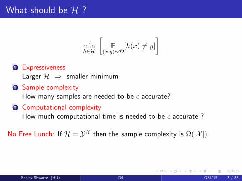
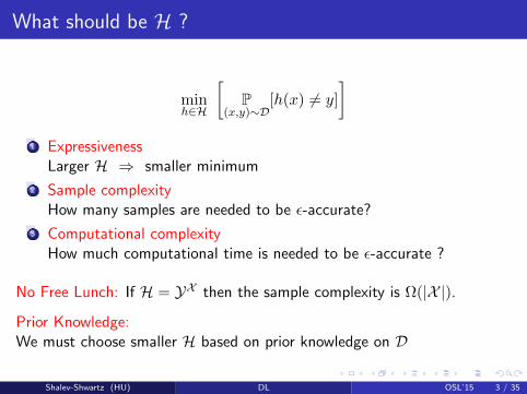
What should be H ?
minh∈H
[P
(x,y)∼D[h(x) 6= y]
]1 Expressiveness
Larger H ⇒ smaller minimum
2 Sample complexityHow many samples are needed to be ε-accurate?
3 Computational complexityHow much computational time is needed to be ε-accurate ?
No Free Lunch: If H = YX then the sample complexity is Ω(|X |).
Prior Knowledge:We must choose smaller H based on prior knowledge on D
Shalev-Shwartz (HU) DL OSL’15 3 / 35

Prior Knowledge
SVM and AdaBoost learn a halfspace on top of features, and most ofthe practical work is on finding good features
Very strong prior knowledge
x
x
Shalev-Shwartz (HU) DL OSL’15 4 / 35
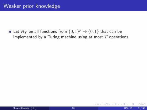
Weaker prior knowledge
Let HT be all functions from 0, 1p → 0, 1 that can beimplemented by a Turing machine using at most T operations.
Very expressive class
Sample complexity ?
Theorem
HT is contained in the class of neural networks of depth O(T ) andsize O(T 2)
The sample complexity of this class is O(T 2)
Shalev-Shwartz (HU) DL OSL’15 5 / 35
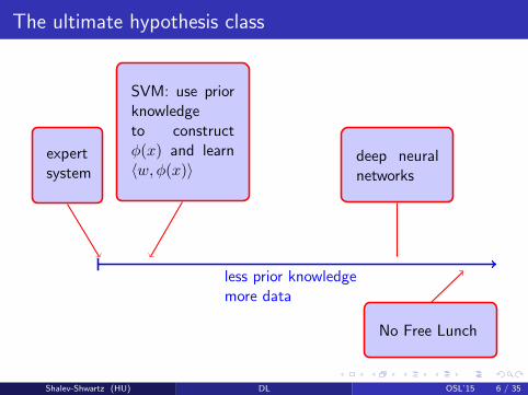
The ultimate hypothesis class
less prior knowledgemore data
expertsystem
SVM: use priorknowledgeto constructφ(x) and learn〈w, φ(x)〉
deep neuralnetworks
No Free Lunch
Shalev-Shwartz (HU) DL OSL’15 6 / 35
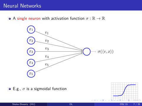
Neural Networks
A single neuron with activation function σ : R→ R
x1
x2
x3
x4
x5
σ(〈v, x〉)
v1
v2
v3
v4
v5
E.g., σ is a sigmoidal function
Shalev-Shwartz (HU) DL OSL’15 7 / 35
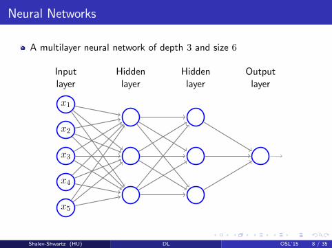
Neural Networks
A multilayer neural network of depth 3 and size 6
x1
x2
x3
x4
x5
Hiddenlayer
Hiddenlayer
Inputlayer
Outputlayer
Shalev-Shwartz (HU) DL OSL’15 8 / 35

Brief history
Neural networks were popular in the 70’s and 80’s
Then, suppressed by SVM and Adaboost on the 90’s
In 2006, several deep architectures with unsupervised pre-traininghave been proposed
In 2012, Krizhevsky, Sutskever, and Hinton significantly improvedstate-of-the-art without unsupervised pre-training
Since 2012, state-of-the-art in vision, speech, and more
Shalev-Shwartz (HU) DL OSL’15 9 / 35

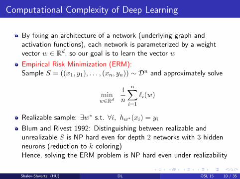
Computational Complexity of Deep Learning
By fixing an architecture of a network (underlying graph andactivation functions), each network is parameterized by a weightvector w ∈ Rd, so our goal is to learn the vector w
Empirical Risk Minimization (ERM):Sample S = ((x1, y1), . . . , (xn, yn)) ∼ Dn and approximately solve
minw∈Rd
1
n
n∑i=1
`i(w)
Realizable sample: ∃w∗ s.t. ∀i, hw∗(xi) = yi
Blum and Rivest 1992: Distinguishing between realizable andunrealizable S is NP hard even for depth 2 networks with 3 hiddenneurons (reduction to k coloring)Hence, solving the ERM problem is NP hard even under realizability
Shalev-Shwartz (HU) DL OSL’15 10 / 35

Computational Complexity of Deep Learning
The argument of Pitt and Valiant (1988)
If it is NP-hard to distinguish realizable from un-realizable samples, thenproperly learning H is hard (unless RP=NP)
Proof: Run the learning algorithm on the empirical distribution over thesample to get h ∈ H with empirical error < 1/n:
If ∀i, h(xi) = yi, return “realizable”
Otherwise, return “unrealizable”
Shalev-Shwartz (HU) DL OSL’15 11 / 35
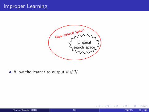
Improper Learning
Originalsearch space
New search space
Allow the learner to output h 6∈ H
The argument of Pitt and Valiant fails because the algorithm mayreturn consistent h even though S is unrealizable by HIs deep learning still hard in the improper model ?
Shalev-Shwartz (HU) DL OSL’15 12 / 35

Improper Learning
Originalsearch space
New search space
Allow the learner to output h 6∈ HThe argument of Pitt and Valiant fails because the algorithm mayreturn consistent h even though S is unrealizable by H
Is deep learning still hard in the improper model ?
Shalev-Shwartz (HU) DL OSL’15 12 / 35

Improper Learning
Originalsearch space
New search space
Allow the learner to output h 6∈ HThe argument of Pitt and Valiant fails because the algorithm mayreturn consistent h even though S is unrealizable by HIs deep learning still hard in the improper model ?
Shalev-Shwartz (HU) DL OSL’15 12 / 35

Hope ...
Generated examples in R150 and passed them through a randomdepth-2 network that contains 60 hidden neurons with the ReLUactivation function.Tried to fit a new network to this data with over-specification factorsof 1, 2, 4, 8
0 0.2 0.4 0.6 0.8 1
·105
0
1
2
3
4
#iterations
MS
E
1248
Shalev-Shwartz (HU) DL OSL’15 13 / 35

How to show hardness of improper learning?
The argument of Pitt and Valiant fails for improper learning becauseimproper algorithms might perform well on unrealizable samples
Key Observation
If a learning algorithm is computationally efficient its output mustcome from a class of “small” VC dimension
Hence, it cannot perform well on “very random” samples
Using the above observation we conclude:
Hardness of distinguishing realizable form “random” samples implieshardness of improper learning of H
Shalev-Shwartz (HU) DL OSL’15 14 / 35
Deep Learning is Hard
Using the new technique and under a natural hardness assumption we canshow:
It is hard to improperly learn intersections of ω(1) halfspaces
It is hard to improperly learn depth ≥ 2 networks with ω(1) neurons,with the threshold or ReLU or sigmoid activation functions
Shalev-Shwartz (HU) DL OSL’15 15 / 35
Theory-Practice Gap
In theory: it is hard to train even depth 2 networks
In practice: Networks of depth 2− 20 are trained successfully
How to circumvent hardness?
Change the problem ...
Add more assumptions
Depart from worst-case analysis
Shalev-Shwartz (HU) DL OSL’15 16 / 35

Theory-Practice Gap
In theory: it is hard to train even depth 2 networks
In practice: Networks of depth 2− 20 are trained successfully
How to circumvent hardness?
Change the problem ...
Add more assumptions
Depart from worst-case analysis
Shalev-Shwartz (HU) DL OSL’15 16 / 35
Theory-Practice Gap
In theory: it is hard to train even depth 2 networks
In practice: Networks of depth 2− 20 are trained successfully
How to circumvent hardness?
Change the problem ...
Add more assumptions
Depart from worst-case analysis
Shalev-Shwartz (HU) DL OSL’15 16 / 35
Theory-Practice Gap
In theory: it is hard to train even depth 2 networks
In practice: Networks of depth 2− 20 are trained successfully
How to circumvent hardness?
Change the problem ...
Add more assumptions
Depart from worst-case analysis
Shalev-Shwartz (HU) DL OSL’15 16 / 35
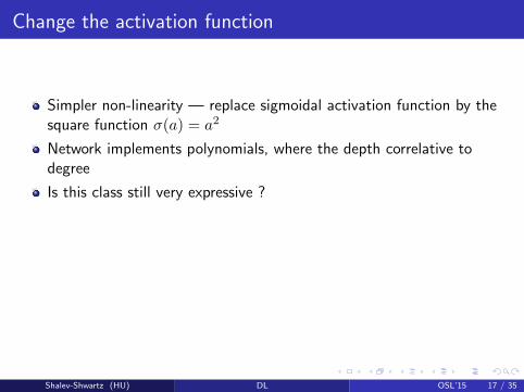
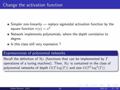
Change the activation function
Simpler non-linearity — replace sigmoidal activation function by thesquare function σ(a) = a2
Network implements polynomials, where the depth correlative todegree
Is this class still very expressive ?
Expressiveness of polynomial networks
Recall the definition of HT (functions that can be implemented by Toperations of a turing machine). Then, HT is contained in the class ofpolynomial networks of depth O(T log(T )) and size O(T 2 log2(T ))
Shalev-Shwartz (HU) DL OSL’15 17 / 35

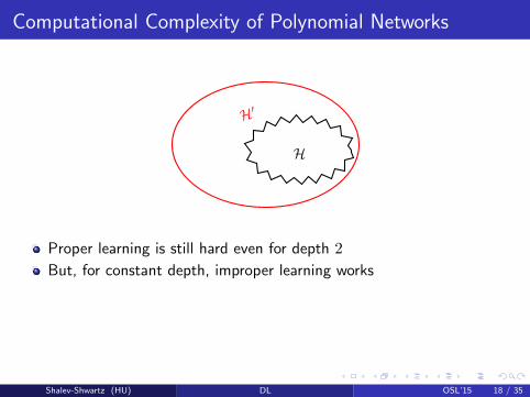
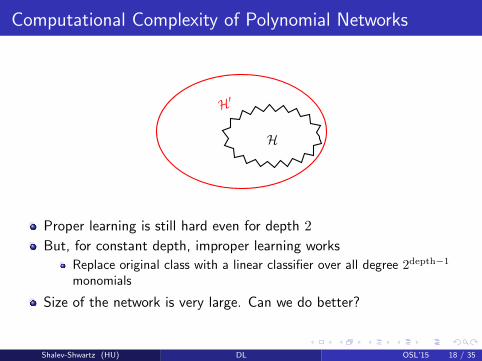
Computational Complexity of Polynomial Networks
H
H′
Proper learning is still hard even for depth 2
But, for constant depth, improper learning works
Replace original class with a linear classifier over all degree 2depth−1
monomials
Size of the network is very large. Can we do better?
Shalev-Shwartz (HU) DL OSL’15 18 / 35
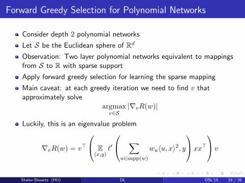
Forward Greedy Selection for Polynomial Networks
Consider depth 2 polynomial networks
Let S be the Euclidean sphere of Rd
Observation: Two layer polynomial networks equivalent to mappingsfrom S to R with sparse support
Apply forward greedy selection for learning the sparse mapping
Main caveat: at each greedy iteration we need to find v thatapproximately solve
argmaxv∈S
|∇vR(w)|
Luckily, this is an eigenvalue problem
∇vR(w) = v>
E(x,y)
`′
∑u∈supp(w)
wu〈u, x〉2, y
xx>
v
Shalev-Shwartz (HU) DL OSL’15 19 / 35
Back to Sigmoidal (and ReLU) Networks
Let Ht,n,L,sig be the class of sigmoidal networks with depth t, size n,and bound L on the `1 norm of the input weights of each neuron
Let Ht,n,poly be defined similarly for polynomial networks
Theorem
∀ε, Ht,n,L,sig ⊂ε Ht log(L(t−log ε)),nL(t−log ε),poly
Corollary
Constant depth sigmoidal networks with L = O(1) are efficientlylearnable !
It is hard to learn polynomial networks of depth Ω(log(d)) and sizeΩ(d)
Shalev-Shwartz (HU) DL OSL’15 20 / 35
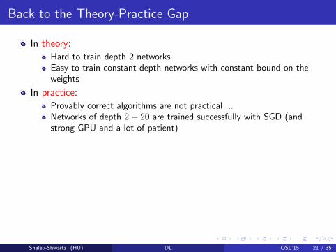
Back to the Theory-Practice Gap
In theory:
Hard to train depth 2 networks
Easy to train constant depth networks with constant bound on theweights
In practice:
Provably correct algorithms are not practical ...Networks of depth 2− 20 are trained successfully with SGD (andstrong GPU and a lot of patient)
How to circumvent hardness?
Change the problem ...
Add more assumptions
Depart from worst-case analysisWhen does SGD work ? Can we make it better ?
Shalev-Shwartz (HU) DL OSL’15 21 / 35

Back to the Theory-Practice Gap
In theory:
Hard to train depth 2 networksEasy to train constant depth networks with constant bound on theweights
In practice:
Provably correct algorithms are not practical ...
Networks of depth 2− 20 are trained successfully with SGD (andstrong GPU and a lot of patient)
How to circumvent hardness?
Change the problem ...
Add more assumptions
Depart from worst-case analysisWhen does SGD work ? Can we make it better ?
Shalev-Shwartz (HU) DL OSL’15 21 / 35
Back to the Theory-Practice Gap
In theory:
Hard to train depth 2 networksEasy to train constant depth networks with constant bound on theweights
In practice:
Provably correct algorithms are not practical ...Networks of depth 2− 20 are trained successfully with SGD (andstrong GPU and a lot of patient)
How to circumvent hardness?
Change the problem ...
Add more assumptions
Depart from worst-case analysisWhen does SGD work ? Can we make it better ?
Shalev-Shwartz (HU) DL OSL’15 21 / 35

Back to the Theory-Practice Gap
In theory:
Hard to train depth 2 networksEasy to train constant depth networks with constant bound on theweights
In practice:
Provably correct algorithms are not practical ...Networks of depth 2− 20 are trained successfully with SGD (andstrong GPU and a lot of patient)
How to circumvent hardness?
Change the problem ...
Add more assumptions
Depart from worst-case analysisWhen does SGD work ? Can we make it better ?
Shalev-Shwartz (HU) DL OSL’15 21 / 35

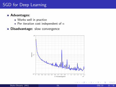
SGD for Deep Learning
Advantages:Works well in practicePer iteration cost independent of n
Disadvantage: slow convergence
0 0.1 0.2 0.3 0.4 0.5 0.6 0.7 0.8 0.9 1 1.1 1.2 1.3 1.4 1.5
·107
10−2
10−1
100
# of backpropagation
obje
ctiv
e
Shalev-Shwartz (HU) DL OSL’15 22 / 35
SGD for Deep Learning
Advantages:Works well in practicePer iteration cost independent of n
Disadvantage: slow convergence
0 0.1 0.2 0.3 0.4 0.5 0.6 0.7 0.8 0.9 1 1.1 1.2 1.3 1.4 1.5
·107
10−2
10−1
100
# of backpropagation
obje
ctiv
e
Shalev-Shwartz (HU) DL OSL’15 22 / 35

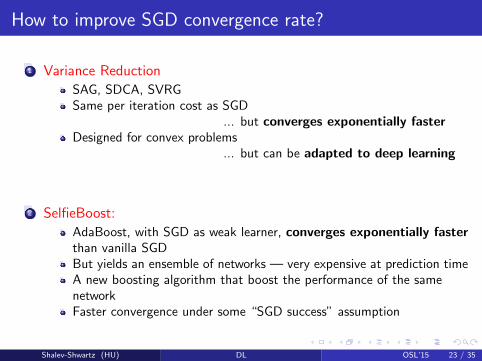
How to improve SGD convergence rate?
1 Variance Reduction
SAG, SDCA, SVRGSame per iteration cost as SGD
... but converges exponentially fasterDesigned for convex problems
... but can be adapted to deep learning
2 SelfieBoost:
AdaBoost, with SGD as weak learner, converges exponentially fasterthan vanilla SGDBut yields an ensemble of networks — very expensive at prediction timeA new boosting algorithm that boost the performance of the samenetworkFaster convergence under some “SGD success” assumption
Shalev-Shwartz (HU) DL OSL’15 23 / 35
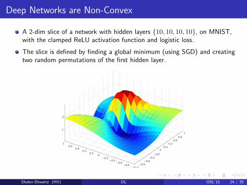
Deep Networks are Non-Convex
A 2-dim slice of a network with hidden layers 10, 10, 10, 10, on MNIST,with the clamped ReLU activation function and logistic loss.
The slice is defined by finding a global minimum (using SGD) and creatingtwo random permutations of the first hidden layer.
−1−0.8−0.6−0.4−0.2
00.2
0.40.6
0.8
1
−1−0.8
−0.6−0.4
−0.20
0.20.4
0.60.8
1
1
2
Shalev-Shwartz (HU) DL OSL’15 24 / 35

But Deep Networks Seem Convex Near a Miminum
Now the slice is based on 2 random points at distance 1 around a globalminimum
−1 −0.8 −0.6 −0.4 −0.20 0.2 0.4 0.6 0.8 1
−1
−0.5
0
0.5
1
4
5
6
7
8
·10−2
Shalev-Shwartz (HU) DL OSL’15 25 / 35
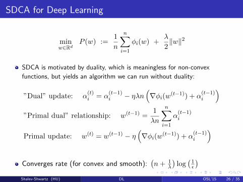
SDCA for Deep Learning
minw∈Rd
P (w) :=1
n
n∑i=1
φi(w) +λ
2‖w‖2
SDCA is motivated by duality, which is meaningless for non-convex
functions, but yields an algorithm we can run without duality:
”Dual” update: α(t)i = α
(t−1)i − ηλn
(∇φi(w(t−1)) + α
(t−1)i
)”Primal dual” relationship: w(t−1) =
1
λn
n∑i=1
α(t−1)i
Primal update: w(t) = w(t−1) − η(∇φi(w(t−1)) + α
(t−1)i
)
Converges rate (for convex and smooth):(n+ 1
λ
)log(1ε
)Shalev-Shwartz (HU) DL OSL’15 26 / 35

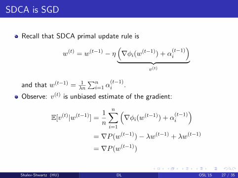
SDCA is SGD
Recall that SDCA primal update rule is
w(t) = w(t−1) − η(∇φi(w(t−1)) + α
(t−1)i
)︸ ︷︷ ︸
v(t)
and that w(t−1) = 1λn
∑ni=1 α
(t−1)i .
Observe: v(t) is unbiased estimate of the gradient:
E[v(t)|w(t−1)] =1
n
n∑i=1
(∇φi(w(t−1)) + α
(t−1)i
)= ∇P (w(t−1))− λw(t−1) + λw(t−1)
= ∇P (w(t−1))
Shalev-Shwartz (HU) DL OSL’15 27 / 35
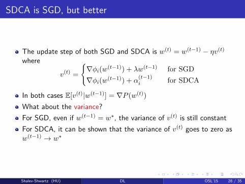
SDCA is SGD, but better
The update step of both SGD and SDCA is w(t) = w(t−1) − ηv(t)where
v(t) =
∇φi(w(t−1)) + λw(t−1) for SGD
∇φi(w(t−1)) + α(t−1)i for SDCA
In both cases E[v(t)|w(t−1)] = ∇P (w(t))
What about the variance?
For SGD, even if w(t−1) = w∗, the variance of v(t) is still constant
For SDCA, it can be shown that the variance of v(t) goes to zero asw(t−1) → w∗
Shalev-Shwartz (HU) DL OSL’15 28 / 35

How to improve SGD?
0 0.1 0.2 0.3 0.4 0.5 0.6 0.7 0.8 0.9 1 1.1 1.2 1.3 1.4 1.5
·107
10−2
10−1
100
# of backpropagation
obje
ctiv
e
Why SGD is slow at the end?
High variance, even close to the optimum
Rare mistakes: Suppose all but 1% of the examples are correctlyclassified. SGD will now waste 99% of its time on examples that arealready correct by the model
Shalev-Shwartz (HU) DL OSL’15 29 / 35
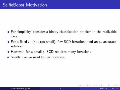
SelfieBoost Motivation
For simplicity, consider a binary classification problem in the realizablecase
For a fixed ε0 (not too small), few SGD iterations find an ε0-accuratesolution
However, for a small ε, SGD requires many iterations
Smells like we need to use boosting ....
Shalev-Shwartz (HU) DL OSL’15 30 / 35

First idea: learn an ensemble using AdaBoost
Fix ε0 (say 0.05), and assume SGD can find a solution with error < ε0quite fast
Lets apply AdaBoost with the SGD learner as a weak learner:
At iteration t, we sub-sample a training set based on a distribution Dt
over [n]We feed the sub-sample to a SGD learner and gets a weak classifier htUpdate Dt+1 based on the predictions of htThe output of AdaBoost is an ensemble with prediction
∑Tt=1 αtht(x)
The celebrated Freund & Schapire theorem states that ifT = O(log(1/ε)) then the error of the ensemble classifier is at most ε
Observe that each boosting iteration involves calling SGD on arelatively small data, and updating the distribution on the entire bigdata. The latter step can be performed in parallel
Disadvantage of learning an ensemble: at prediction time, we need toapply many networks
Shalev-Shwartz (HU) DL OSL’15 31 / 35
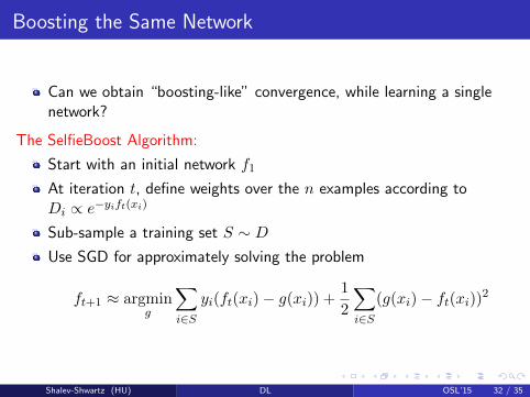
Boosting the Same Network
Can we obtain “boosting-like” convergence, while learning a singlenetwork?
The SelfieBoost Algorithm:
Start with an initial network f1
At iteration t, define weights over the n examples according toDi ∝ e−yift(xi)
Sub-sample a training set S ∼ DUse SGD for approximately solving the problem
ft+1 ≈ argming
∑i∈S
yi(ft(xi)− g(xi)) +1
2
∑i∈S
(g(xi)− ft(xi))2
Shalev-Shwartz (HU) DL OSL’15 32 / 35

Analysis of the SelfieBoost Algorithm
Lemma: At each iteration, with high probability over the choice of S,there exists a network g with objective value of at most −1/4
Theorem: If at each iteration, the SGD algorithm finds a solutionwith objective value of at most −ρ, then after
log(1/ε)
ρ
SelfieBoost iterations the error of ft will be at most ε
To summarize: we have obtained log(1/ε) convergence assuming thatthe SGD algorithm can solve each sub-problem to a fixed accuracy(which seems to hold in practice)
Shalev-Shwartz (HU) DL OSL’15 33 / 35

SelfieBoost vs. SGD
On MNIST dataset, depth 5 network
0 0.1 0.2 0.3 0.4 0.5 0.6 0.7 0.8 0.9 1 1.1 1.2 1.3 1.4 1.5
·107
10−4
10−3
10−2
10−1
100
# of backpropagation
erro
r
SGDSelfieBoost
Shalev-Shwartz (HU) DL OSL’15 34 / 35
Summary
Why deep networks: Deep networks are the ultimate hypothesis classfrom the statistical perspective
Why not: Deep networks are a horrible class from the computationalpoint of view
This work: Deep networks with bounded depth and `1 norm are nothard to learn
Provably correct theoretical algorithms are in general not practical.
Why SGD works ???
How can we make it better ?
Shalev-Shwartz (HU) DL OSL’15 35 / 35
Top Related