


Languages
Pages
Legal


On measurement and modelling of 2D magnetization and
magnetostriction of SiFe sheets
Anders Lundgren
Royal Institute of Technology
Electric Power Engineering
Stockholm 1999

Anders Lundgren On measurement and modelling of 2D magnetization and magnetostriction of SiFe sheets

TRITA-EEA-9901
ISSN 1100-1593
Department of Electric Power Engineering
Royal Institute of Technology
SE-100 44 Stockholm
SWEDEN

On measurement and modelling of 2D magnetization and
magnetostriction of SiFe sheets
Anders Lundgren
Royal Institute of Technology
Electric Power Engineering
Stockholm 1999

Akademisk avhandling som med tillst�and av Kungl Tekniska H�ogskolan framl�agges
till o�entlig granskning f�or avl�aggande av teknisk doktorsexamen m�andagen den
21 juni 1999 kl 14.00i Kollegiesalen, Administrationsbyggnaden, Kungl Tekniska
H�ogskolan, Valhallav�agen 79, Stockholm.
TRITA-EEA-9901
ISSN 1100-1593
c Anders Lundgren, 1999
KTH Reprocentral, Stockholm 1999

Abstract
The development and technological aspects of a 2D magnetization and magne-
tostriction measurement setup are documented and described. Local magnetic in-
tensity and ux density are measured with Rogowski and material encircling coils.
In-plane strain is measured with a homodyne laser interferometer. Measured and
processed time-domain signals, hysteresis plots and signature data such as loss are
presented by an e�cient and communicative interface. Measurements on quadratic
silicon iron sheet samples are included. Material types tested on the setup are with
non-oriented and oriented textures. Possible excitations include uniaxial alternat-
ing magnetic �eld in the rolling and transverse directions between 10 and 300 Hz at
least. Rotational excitations are possible at least for the non-oriented and conven-
tional grain-oriented types. The value of the setup lies in the possibility of using it
for routine measurements on samples.
The interplay between mathematical modelling and physical experimenting is de-
scribed. Investigations by algebraic and numerical methods are done to �nd a pos-
sible way to parameterize material behaviour and include this behaviour in �nite
element programs. On the basis of a proposed one-dimensional nonlinear model,
algorithms are devised to compute magnetostrictive responses to uniaxially alter-
nating magnetic �elds. An experimental FEM program to calculate strain �elds
from inhomogeneous magnetization is developed. Its use for investigation of sample
behaviour during the operation of the setup is shown. The value of the proposed
modelling methodology lies in the study of possibilities of lowering the production
of magnetostrictive vibration in transformer, motor and generator cores.
IEEE index terms: Magnetostriction, silicon steel, magnetic cores, strain, inter-
ferometry, magnetic anisotropy, magnetic �elds, magnetic measurements, magne-
toelasticity, nonlinear magnetics, power transformers, power distribution acoustic
noise, �nite element methods.
TRITA-EEA-9901
ISSN 1100-1593

Acknowledgements
I would like to thank the members of the reference committee, Jan Anger (ABB
Transformers), Thomas Edstr�om (ABB Corporate Research) and Birger Nilsson
(ABB Corporate Research) and Elektra programmemanager Sten Bergman (Elforsk
AB) for their work in supporting this project.
On the department side I owe thanks to the project manager G�oran Engdahl for
energizing the project, applying for funding and proofreading. Head of department
Roland Eriksson is thanked for employing me and for administering the �nances and
agreements. I especially wish to thank former research associate Anders Bergqvist
for many stimulating discussions and collaborations. I thank Olle Br�annvall, G�ote
Bergh and Yngve Eriksson for making parts to the experimental setup and trans-
porting it. I send greetings to friendly department colleagues Eckart Nipp, Niklas
Magnusson, Fredrik Stillesj�o, Mats Kvarngren and Anders Helgesson.
I �nally express heartily thanks to my girlfriend Cecilia H�aggmark for her encour-
agement, proofreading and general support.
Anders Lundgren
i

Contents
1 Introduction 1
1.1 Overview . . . . . . . . . . . . . . . . . . . . . . . . . . . . . . . . . 1
1.2 Motivation and goals . . . . . . . . . . . . . . . . . . . . . . . . . . . 3
1.3 Credits . . . . . . . . . . . . . . . . . . . . . . . . . . . . . . . . . . . 4
1.4 Literature review . . . . . . . . . . . . . . . . . . . . . . . . . . . . . 5
1.4.1 Magnetic hysteresis models . . . . . . . . . . . . . . . . . . . 5
1.4.2 Magnetostriction . . . . . . . . . . . . . . . . . . . . . . . . . 6
1.4.3 Stress dependence . . . . . . . . . . . . . . . . . . . . . . . . 11
1.4.4 Measurement methods . . . . . . . . . . . . . . . . . . . . . . 12
1.4.5 Numerics . . . . . . . . . . . . . . . . . . . . . . . . . . . . . 14
1.4.6 Technology . . . . . . . . . . . . . . . . . . . . . . . . . . . . 15
2 Measurement system 17
2.1 Introduction . . . . . . . . . . . . . . . . . . . . . . . . . . . . . . . . 17
2.2 Purposes . . . . . . . . . . . . . . . . . . . . . . . . . . . . . . . . . . 18
2.3 Drawing and design system . . . . . . . . . . . . . . . . . . . . . . . 19
2.4 Data acquisition programs . . . . . . . . . . . . . . . . . . . . . . . . 21
ii
2.5 Magnetic circuit . . . . . . . . . . . . . . . . . . . . . . . . . . . . . 23
2.6 Excitation frequency limits . . . . . . . . . . . . . . . . . . . . . . . 23
2.7 Voltage or current sti� ampli�er . . . . . . . . . . . . . . . . . . . . 28
2.8 B-coils . . . . . . . . . . . . . . . . . . . . . . . . . . . . . . . . . . . 29
2.9 Calibration of the H-coil . . . . . . . . . . . . . . . . . . . . . . . . . 31
2.10 Measurement table . . . . . . . . . . . . . . . . . . . . . . . . . . . . 32
2.10.1 Support placement . . . . . . . . . . . . . . . . . . . . . . . . 33
2.10.2 Optic component placement . . . . . . . . . . . . . . . . . . . 33
2.11 Vibration of material . . . . . . . . . . . . . . . . . . . . . . . . . . . 34
2.12 Digital control issues . . . . . . . . . . . . . . . . . . . . . . . . . . . 35
2.13 Strain measurement by interferometry . . . . . . . . . . . . . . . . . 36
2.14 Stress in uence, frame e�ect . . . . . . . . . . . . . . . . . . . . . . . 37
2.15 Yoke design . . . . . . . . . . . . . . . . . . . . . . . . . . . . . . . . 37
2.16 Magnetic sensor design . . . . . . . . . . . . . . . . . . . . . . . . . . 38
2.17 Temperature drift . . . . . . . . . . . . . . . . . . . . . . . . . . . . 39
2.18 Signal conditioning and Nyquist limit . . . . . . . . . . . . . . . . . 39
2.19 Signal bu�ering . . . . . . . . . . . . . . . . . . . . . . . . . . . . . . 41
2.20 Measurement coil misalignments . . . . . . . . . . . . . . . . . . . . 43
2.21 Using the measurement system . . . . . . . . . . . . . . . . . . . . . 43
2.21.1 Magnetic measurements . . . . . . . . . . . . . . . . . . . . . 43
2.21.2 Peak ux . . . . . . . . . . . . . . . . . . . . . . . . . . . . . 44
2.21.3 Measurement procedure . . . . . . . . . . . . . . . . . . . . . 44
3 Interferometer 46
iii
3.1 Introduction . . . . . . . . . . . . . . . . . . . . . . . . . . . . . . . . 46
3.2 Homodyne interferometry . . . . . . . . . . . . . . . . . . . . . . . . 48
3.3 Heterodyne interferometry . . . . . . . . . . . . . . . . . . . . . . . . 49
3.4 Interferometer alignment . . . . . . . . . . . . . . . . . . . . . . . . . 49
3.5 Doppler e�ect . . . . . . . . . . . . . . . . . . . . . . . . . . . . . . . 51
3.6 Motion of measurement table . . . . . . . . . . . . . . . . . . . . . . 52
3.7 Laser . . . . . . . . . . . . . . . . . . . . . . . . . . . . . . . . . . . . 58
3.8 The acousto-optic modulator . . . . . . . . . . . . . . . . . . . . . . 60
3.9 Beam splitters and prisms . . . . . . . . . . . . . . . . . . . . . . . . 62
3.10 Interference �lter . . . . . . . . . . . . . . . . . . . . . . . . . . . . . 63
3.11 Photodiode . . . . . . . . . . . . . . . . . . . . . . . . . . . . . . . . 63
3.12 Demodulator . . . . . . . . . . . . . . . . . . . . . . . . . . . . . . . 65
3.13 Interferometer type . . . . . . . . . . . . . . . . . . . . . . . . . . . . 65
3.14 Re ector placements and properties . . . . . . . . . . . . . . . . . . 65
4 Strain analysis 68
4.1 Introduction . . . . . . . . . . . . . . . . . . . . . . . . . . . . . . . . 68
4.2 De�nitions of observables . . . . . . . . . . . . . . . . . . . . . . . . 68
4.2.1 2D strain measurement analysis . . . . . . . . . . . . . . . . . 73
4.2.2 Deformation of volume elements . . . . . . . . . . . . . . . . 76
4.3 Stress and 3D elastic material relations . . . . . . . . . . . . . . . . . 77
4.4 2D elastic material modelling . . . . . . . . . . . . . . . . . . . . . . 80
4.4.1 Magnetostriction components and constitutive relations . . . 80
4.4.2 Elasticity and compliance matrices . . . . . . . . . . . . . . . 85
iv

4.5 Equations of equilibrium and motion . . . . . . . . . . . . . . . . . . 87
4.5.1 Force equilibrium . . . . . . . . . . . . . . . . . . . . . . . . . 87
4.5.2 Torque equilibrium . . . . . . . . . . . . . . . . . . . . . . . . 88
4.5.3 Equations of motion, coordinate types . . . . . . . . . . . . . 89
4.5.4 Translatory and rotatory equations of motion . . . . . . . . . 89
4.5.5 Body forces . . . . . . . . . . . . . . . . . . . . . . . . . . . . 90
4.6 Magnetic stress . . . . . . . . . . . . . . . . . . . . . . . . . . . . . . 91
5 Models of magnetostriction 93
5.1 The interplay between mathematical modeling and physical experi-
menting . . . . . . . . . . . . . . . . . . . . . . . . . . . . . . . . . . 93
5.2 Continuum model . . . . . . . . . . . . . . . . . . . . . . . . . . . . . 94
5.3 Butter y loops . . . . . . . . . . . . . . . . . . . . . . . . . . . . . . 96
5.4 Rate-dependency model . . . . . . . . . . . . . . . . . . . . . . . . . 97
5.5 Simple 2D magnetostriction models . . . . . . . . . . . . . . . . . . . 98
5.6 Magnetoviscoelastic models . . . . . . . . . . . . . . . . . . . . . . . 98
5.6.1 Quasistatic linear case . . . . . . . . . . . . . . . . . . . . . . 99
5.6.2 Rate-dependent linear case . . . . . . . . . . . . . . . . . . . 99
5.6.3 Rate-dependent nonlinear case . . . . . . . . . . . . . . . . . 100
5.7 Model incorporation in plane stress calculations . . . . . . . . . . . . 101
5.7.1 Nonlinear dispersion . . . . . . . . . . . . . . . . . . . . . . . 103
5.8 Macroscopic magnetostrictive response . . . . . . . . . . . . . . . . . 103
5.9 Identi�cation of parameters . . . . . . . . . . . . . . . . . . . . . . . 104
5.9.1 Magnetostrictive incompressibility . . . . . . . . . . . . . . . 104
v

5.10 Magnetoelastic shear modulus . . . . . . . . . . . . . . . . . . . . . . 106
5.11 Vector and tensor transformation . . . . . . . . . . . . . . . . . . . . 107
5.12 Magnetic stress alternatives . . . . . . . . . . . . . . . . . . . . . . . 108
5.13 Compliance transformation . . . . . . . . . . . . . . . . . . . . . . . 109
5.14 Piezomagnetism . . . . . . . . . . . . . . . . . . . . . . . . . . . . . . 111
5.15 Physical models . . . . . . . . . . . . . . . . . . . . . . . . . . . . . . 114
5.16 Material structure . . . . . . . . . . . . . . . . . . . . . . . . . . . . 115
5.16.1 Texture . . . . . . . . . . . . . . . . . . . . . . . . . . . . . . 115
5.16.2 Transformer iron qualities . . . . . . . . . . . . . . . . . . . . 116
5.17 Micromagnetic cause of magnetostriction . . . . . . . . . . . . . . . . 116
5.18 Domains in soft magnetic materials . . . . . . . . . . . . . . . . . . . 117
5.19 Domain walls and magnetostriction . . . . . . . . . . . . . . . . . . . 119
5.20 Domain types . . . . . . . . . . . . . . . . . . . . . . . . . . . . . . . 120
6 Magnetic �nite element analysis 123
6.1 Introduction . . . . . . . . . . . . . . . . . . . . . . . . . . . . . . . . 123
6.2 Coupling . . . . . . . . . . . . . . . . . . . . . . . . . . . . . . . . . . 124
6.3 General motivation and conditions for simulations with computer . . 124
6.4 2D magnetostatic �nite element method . . . . . . . . . . . . . . . . 125
6.4.1 A linear isotropic scalar potential problem . . . . . . . . . . . 125
6.4.2 Discretization . . . . . . . . . . . . . . . . . . . . . . . . . . . 126
6.4.3 Single triangle element . . . . . . . . . . . . . . . . . . . . . . 127
6.4.4 System of linear equations . . . . . . . . . . . . . . . . . . . . 128
6.4.5 Hollow cylinder test case . . . . . . . . . . . . . . . . . . . . . 129
vi

6.4.6 A nonlinear isotropic formalism . . . . . . . . . . . . . . . . . 130
6.5 3D isotropic formulation . . . . . . . . . . . . . . . . . . . . . . . . . 133
6.6 3D anisotropic formulation . . . . . . . . . . . . . . . . . . . . . . . 134
7 Mechanical �nite element analysis 136
7.1 Introduction . . . . . . . . . . . . . . . . . . . . . . . . . . . . . . . . 136
7.2 E�ect of inhomogeneous magnetization . . . . . . . . . . . . . . . . . 136
7.3 Mechanical simulation method . . . . . . . . . . . . . . . . . . . . . 139
7.4 Results and interpretation . . . . . . . . . . . . . . . . . . . . . . . . 139
7.5 Strain �eld calculation method . . . . . . . . . . . . . . . . . . . . . 142
7.5.1 Plane stress constitutive relation . . . . . . . . . . . . . . . . 142
7.5.2 Finite element method . . . . . . . . . . . . . . . . . . . . . . 142
7.6 Bending . . . . . . . . . . . . . . . . . . . . . . . . . . . . . . . . . . 146
7.6.1 Magnetic �eld and force calculation . . . . . . . . . . . . . . 147
7.6.2 Bending formulation . . . . . . . . . . . . . . . . . . . . . . . 147
7.6.3 Extra details . . . . . . . . . . . . . . . . . . . . . . . . . . . 150
7.6.4 Nonmagnetized case . . . . . . . . . . . . . . . . . . . . . . . 157
7.6.5 Rolling direction magnetization . . . . . . . . . . . . . . . . . 157
7.6.6 Transversal magnetization . . . . . . . . . . . . . . . . . . . . 158
7.6.7 Experiments . . . . . . . . . . . . . . . . . . . . . . . . . . . 158
8 Measurement and veri�cation 163
8.1 Introduction . . . . . . . . . . . . . . . . . . . . . . . . . . . . . . . . 163
8.2 Experiments . . . . . . . . . . . . . . . . . . . . . . . . . . . . . . . . 164
8.3 Data processing and nonlinear model . . . . . . . . . . . . . . . . . . 164
vii

8.4 Frequency dependence . . . . . . . . . . . . . . . . . . . . . . . . . . 169
8.5 2D model from measurements . . . . . . . . . . . . . . . . . . . . . . 169
8.6 Magnetization measurements . . . . . . . . . . . . . . . . . . . . . . 172
9 Conclusions and future work 175
9.1 Conclusions . . . . . . . . . . . . . . . . . . . . . . . . . . . . . . . . 175
9.1.1 Setup uses . . . . . . . . . . . . . . . . . . . . . . . . . . . . . 175
9.1.2 Sample �eld calculation . . . . . . . . . . . . . . . . . . . . . 176
9.1.3 Bending . . . . . . . . . . . . . . . . . . . . . . . . . . . . . . 176
9.1.4 Magnetostriction harmonics . . . . . . . . . . . . . . . . . . . 176
9.2 Future work . . . . . . . . . . . . . . . . . . . . . . . . . . . . . . . . 177
9.2.1 SST improvement . . . . . . . . . . . . . . . . . . . . . . . . 177
9.2.2 Magnetoelastic FEM program development . . . . . . . . . . 177
9.2.3 Magnetostriction measurements . . . . . . . . . . . . . . . . . 178
10 List of symbols 179
11 List of units 185
A Design drawings 196
viii

List of Figures
2.1 Sample support table (not hatched) with yokes (hatched). See Fig.
3.1 for its placement in the setup. . . . . . . . . . . . . . . . . . . . . 24
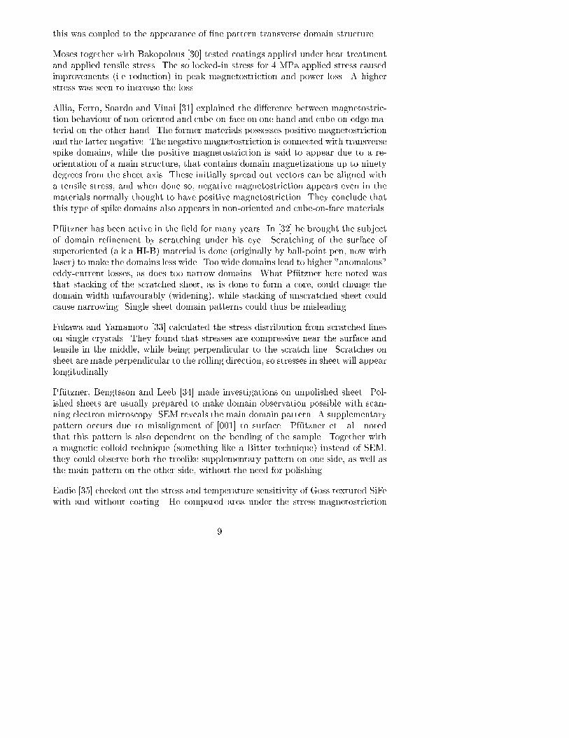
2.2 Magnetic sensors, split sketch. . . . . . . . . . . . . . . . . . . . . . . 25
2.3 Block schematic of electric part of measurement system. . . . . . . . 26
2.4 The magnetic yoke con�guration. Dimensions in mm. . . . . . . . . 26
2.5 One H-coil wound from up to down around a nonmagnetic plate. Hall
probe positions for calibration are marked with circles. Dimensions
in mm. . . . . . . . . . . . . . . . . . . . . . . . . . . . . . . . . . . . 31
3.1 Overview of interferometer . . . . . . . . . . . . . . . . . . . . . . . . 47
3.2 Actual IFM setup . . . . . . . . . . . . . . . . . . . . . . . . . . . . . 48
3.3 The ray in a 90� prism mirrored into a straight ray through a cube. 66
4.1 Relative displacement of length element . . . . . . . . . . . . . . . . 69
4.2 Interpretation of displacement gradient decomposition . . . . . . . . 70
4.3 Interpretation of relative displacement decomposition . . . . . . . . . 71
4.4 Normal strains and shear angle �+ � . . . . . . . . . . . . . . . . . 72
4.5 Polar plot of �011(') and �012(') . . . . . . . . . . . . . . . . . . . . . 74
4.6 90� antisymmetry of shear strains. . . . . . . . . . . . . . . . . . . . 75
ix

4.7 180� symmetry of normal strains . . . . . . . . . . . . . . . . . . . . 75
4.8 Mohr's circle for normal and shear strain in the xy plane. The xy
plane is perpendicular to a principal strain direction. 'p is the anglefrom the x-direction to the direction of the principal strain �1. . . . 76
4.9 Mohr's circles for a complete strain state, three planes perpendicular
to each other and to principal directions. . . . . . . . . . . . . . . . . 77
4.10 Moment equilibrium on an area element . . . . . . . . . . . . . . . . 78
4.11 Normal elastic compliance as function of angle of uniaxial stress to
rolling direction. . . . . . . . . . . . . . . . . . . . . . . . . . . . . . 81
4.12 Orthogonal elastic compliance as function of angle of uniaxial stress
to rolling direction. . . . . . . . . . . . . . . . . . . . . . . . . . . . . 82
4.13 Shear elastic compliance coe�cients as functions of angle of uniaxial
stress to rolling direction. . . . . . . . . . . . . . . . . . . . . . . . . 83
4.14 Uniaxial stress � applied obliquely to a texture. Shows rotation of
the principal strain system �1; �2 compared to the principal stress
system. . . . . . . . . . . . . . . . . . . . . . . . . . . . . . . . . . . 83
4.15 Left: Force on element are from stresses �; � and body force fb.Right: Torque on element are from shear stresses � and body torqueTb. . . . . . . . . . . . . . . . . . . . . . . . . . . . . . . . . . . . . . 88
5.1 Butter y loops of negative valued �Mx vs. Bx and positive valued �My
vs. By. . . . . . . . . . . . . . . . . . . . . . . . . . . . . . . . . . . . 95
5.2 Normal magnetoelastic compliance as function of angle of magnetic
stress to rolling direction. . . . . . . . . . . . . . . . . . . . . . . . . 112
5.3 Orthogonal (to magnetic stress) magnetoelastic compliance as func-
tion of angle of magnetic stress to rolling direction. . . . . . . . . . . 112
5.4 Shear magnetoelastic compliance coe�cients as function of angle of
magnetic wtress to rolling direction. . . . . . . . . . . . . . . . . . . 113
5.5 (110)[001] crystal orientation. RD is rolling direction and TD is
transverse direction of the sheet. . . . . . . . . . . . . . . . . . . . . 115
5.6 Main stripe domains with supplementary lancet domains. . . . . . . 121
x

5.7 Lancet domain viewed from the side. . . . . . . . . . . . . . . . . . . 121
6.1 Equipotential lines for the magnetic scalar potential. Sample mag-
netized in the rolling (x) direction. Oriented material. . . . . . . . . 135
6.2 Equipotential lines for the magnetic scalar potential. Sample mag-
netized in the transversal (y) direction. Oriented material. . . . . . . 135
7.1 Magni�ed (factor 5000) deformation of sheet from ux density vec-
tors. Nonoriented material. . . . . . . . . . . . . . . . . . . . . . . . 138
7.2 Total strain sx and magnetostrictive strain sMx in the measurement
area. Nonoriented material. . . . . . . . . . . . . . . . . . . . . . . . 139
7.3 Magni�ed (factor 50000) deformation of sheet at ux peak time when
x-magnetized. Flux density vectors drawn. Undeformed boundary
dash-dotted. Oriented material. . . . . . . . . . . . . . . . . . . . . . 140
7.4 Magni�ed (factor 50000) deformation of sheet at ux peak time when
y-magnetized. Flux density vectors drawn. Undeformed boundary
dash-dotted. Oriented material. . . . . . . . . . . . . . . . . . . . . . 141
7.5 Geometry for the cut y = 0 in m with gravity as only load. Deforma-
tion of sheet magni�ed with factor 50. Undeformed sheet dash-dotted.148
7.6 Equilines of de ection (solid) for B�0 case. Outlines of pole surfaces(dash-dotted). . . . . . . . . . . . . . . . . . . . . . . . . . . . . . . . 150
7.7 Geometry in m for the cut y = 0 when x-magnetized. Deforma-
tion of sheet magni�ed with factor 50. Flux density vectors drawn.
Undeformed sheet dash-dotted. . . . . . . . . . . . . . . . . . . . . . 158
7.8 Equilines of de ection (solid) when x-magnetized. Outlines of pole
surfaces (dash-dotted). . . . . . . . . . . . . . . . . . . . . . . . . . . 159
7.9 Geometry in m for the cut x = 0 when y-magnetized. De ection of
sheet magni�ed with factor 50. Flux density vectors drawn. Unde-
formed sheet dash-dotted. . . . . . . . . . . . . . . . . . . . . . . . . 160
7.10 Equilines of de ection (solid) when y-magnetized. Outlines of pole
surfaces (dash-dotted). . . . . . . . . . . . . . . . . . . . . . . . . . 161
7.11 Experimental setup . . . . . . . . . . . . . . . . . . . . . . . . . . . . 162
xi
8.1 Measured (solid) and simulated (dash-dotted) B2(t). . . . . . . . . . 165
8.2 Measured (solid) and simulated (dash-dotted) �M (t). . . . . . . . . . 166
8.3 Measured butter y loops of �My vs. By, solid, and single-valued �tted
curve, dash-dotted. . . . . . . . . . . . . . . . . . . . . . . . . . . . 166
8.4 Magnetostriction curves, measured (solid) and simulated with non-
linear model (dash-dotted). . . . . . . . . . . . . . . . . . . . . . . . 167
8.5 Magnetostriction curves, measured (solid) and simulated with non-
linear model (dash-dotted). . . . . . . . . . . . . . . . . . . . . . . . 168
8.6 Magnetostriciton curves, measured (solid) and simulated with linear
model (dash-dotted). . . . . . . . . . . . . . . . . . . . . . . . . . . . 170
8.7 Magnetostriction curves, measured (solid) and simulated with linear
model (dash-dotted). . . . . . . . . . . . . . . . . . . . . . . . . . . 171
8.8 Flux density [T] in rolling direction versus �eld strength [A/m] in
rolling direction. Oriented material. . . . . . . . . . . . . . . . . . . 173
8.9 Flux density [T] in transverse direction versus �eld strength [A/m]
in transverse direction. Oriented material. . . . . . . . . . . . . . . . 173
8.10 Flux density [T] locus. Transverse direction is y-axis and rolling
direction is x-axis. Oriented material. . . . . . . . . . . . . . . . . . 174
8.11 Field strength [A/m] locus. Transverse direction is y-axis and rolling
direction is x-axis. Oriented material. . . . . . . . . . . . . . . . . . 174
A.1 Optic component placement with possible double interferometers . . 197
A.2 Closeup of single interferometer with sample side dimension . . . . . 198
A.3 Side view of interferometer (possibly dual), arm with AOM . . . . . 199
A.4 Side view of interferometer (possibly dual), arm with laser head . . . 199
A.5 Laser mount . . . . . . . . . . . . . . . . . . . . . . . . . . . . . . . . 200
A.6 Custom tapped rod, for optic rail on diabase spacer fastening . . . . 201
A.7 Acoustooptic modulator, fastening on translation stage . . . . . . . . 201
xii

A.8 Baseplate for AOM . . . . . . . . . . . . . . . . . . . . . . . . . . . . 202
A.9 Diabase spacers . . . . . . . . . . . . . . . . . . . . . . . . . . . . . . 203
A.10 Sample support . . . . . . . . . . . . . . . . . . . . . . . . . . . . . . 204
A.11 Tall laminated yoke . . . . . . . . . . . . . . . . . . . . . . . . . . . . 205
A.12 Short laminated yoke . . . . . . . . . . . . . . . . . . . . . . . . . . . 205
A.13 Spacer between yokes . . . . . . . . . . . . . . . . . . . . . . . . . . 206
A.14 Yoke pair assembly . . . . . . . . . . . . . . . . . . . . . . . . . . . . 206
A.15 Table top with tapped mount holes . . . . . . . . . . . . . . . . . . . 207
A.16 Experiment table . . . . . . . . . . . . . . . . . . . . . . . . . . . . . 208
A.17 Table top support . . . . . . . . . . . . . . . . . . . . . . . . . . . . 209
xiii

List of Tables
2.1 Calibration factor as function of calibrating Hall probe position. . . 32
7.1 Dynamic normal strains in x-direction when x-magnetized. . . . . . 141
7.2 Dynamic normal strains in y-direction when y-magnetized. . . . . . 142
7.3 Rotations when not magnetized . . . . . . . . . . . . . . . . . . . . . 157
7.4 Rotations when x-magnetized . . . . . . . . . . . . . . . . . . . . . . 159
7.5 Rotations when y-magnetized . . . . . . . . . . . . . . . . . . . . . . 160
7.6 Experimental results . . . . . . . . . . . . . . . . . . . . . . . . . . . 161
xiv

Chapter 1
Introduction
1.1 Overview
This book is organized as follows.
Chapter 1 contains this overview section, the motivation and goals of the project
behind this book and a credits section. It also contains an article literature review
on the subject of magnetostriction of silicon-iron and related subjects such as mag-
netization behaviour, ux distribution, hysteresis and magnetic domain processes.
Chapter 2 contains a description of the design of a measurement system that can
make 2D magnetic measurements and 1D magnetostriction measurements of sheet
samples. The setup can be called a rotational single sheet tester (RSST), because
the magnetic �eld vectors can be made to rotate in the plane of the sheet. This
chapter also gives some operation guidelines of the RSST.
Chapter 3 contains a description of the interferometer that is used with the RSST to
measure strain. The interferometer was built from basic parts to suit the geometry
of the RSST. This also meant that the time signal from the photodetector easily
could be extracted and correlated with the magnetic time signals. This chapter
also contains a section on how to align the reference and measurement beams to get
interference and make measurements possible. Furthermore, there are discussions
on measurement error causes, particularly the motion of the table top on which the
interferometer is mounted and unwanted rotations(tilts) of the re ecting prisms
mounted on the sample.
1
Chapter 4 states and illustrates the basic de�nitions of displacement, rotation and
strain. The strain component dependence of choice of coordinate system is treated.
Simple elastic material models are reviewed and a magnetostrictive constitutive re-
lation is proposed by analogy. The concept of a magnetic stress tensor as a variable
for parameterizing measurements of magnetostrictive strain versus magnetic �eld
is introduced.
Chapter 5 describes dispersive lag models of magnetostriction suitable for inclusion
in computer programs. Directional dependence of uniaxial response shows the
possibility of including anisotropic materials and gives a guide how to determine
parameters from measurements. The chapter also presents an overview of physical
descriptions of material microstructure and magnetic domains with focus on the
signi�cance to magnetostriction.
Chapter 6 describes the mathematical details of how to discretize a 2D magnetic
scalar potential problem with a �nite element method. The procedure of setting
up a linear equation system for solution with some acquired solver is shown. The
iterated procedure necessary for a nonlinear problem is treated. Scalar potential
formulations suitable for 3D problems are stated. The application of a FEM pro-
gram for solving the magnetic �eld distribution inside the sheet sample is shown.
Chapter 7 describes the mathematical details and algorithms of how to discretize
linear plane stress and thin plate bending problems by �nite element methods.
Every step before using a commercial or free equation system solver is dealt with.
The FEM programs built have been applied to investigate the strain �eld in the
sample, the percentages of elastic strain and magnetostrictive strain in measured
strain and possible rotations of sample re ectors due to sample bending when no
sample support table is used.
Chapter 8 is devoted to the question of how to represent measured nonlinear mag-
netostriction data. The representation method is expansion of a single valued mag-
netostriction in a third order polynomial of the magnetic stress tensor introduced
earlier. The double valued magnetostriction as a function of the magnetic stress is
represented in the frequency domain by a second order transfer function multiplied
by the single valued magnetostriction. Parameter extraction from and comparisons
with magnetostriction measured transversely to rolling direction of a sheet excited
with a �eld strength transversely to rolling direction are shown.
Chapter 9 sums up the developments presented and their strengths and weaknesses.
The path remaining to go to achieve perfection both with measurement hardware
and modelling software is discussed.
2

1.2 Motivation and goals
A signi�cant di�erence in sound level is found between di�erent designs of mag-
netic devices. To understand which parts of the magnetic circuit that are of main
importance to sound generation more complete and accurate models are needed
than the ones used today. The joints in magnetic cores are of special interest to
study because no explanation of the strong in uence of magnetostriction there has
been found. Today no tool exists to model in three dimensions all angle dependent
magnetic properties, including magnetostriction and mechanical stress dependence.
This has been the driving force behind the project, on which the book is based.
The conditions for the models are set by the magnetic design. The project goal
was that the models should be possible to apply to a power transformer, where the
noise caused by magnetostriction is a technically and commercially important prob-
lem. The ultimate goal was that three-dimensional magnetomechanical continuum-
modelling of cores made of oriented silicon iron sheets should be made possible.
This model should include non-linearity, anisotropy and hysteresis, all in a macro-
scopic sense. The models obtained were to be well adapted to a continuum theory
for the vibration of these sheets. Discretization of the continuum problem was then
carried out with the �nite element method, the algorithms of which was imple-
mented in computer programs.
The viewpoint taken in the project was phenomenological. Model development
required methods to collect needed experimental data. Biaxial strain in electric
steel could be measured by laser interferometry under rotating magnetic �elds.
Local magnetic �eld strength and ux density was simultaneously measured. The
integration of the model in �nite-element-software was adapted to the simulation
of samples and cores.
Experimental data covering two-dimensional magnetization excitations and mag-
netostriction responses was collected from a custom designed measurement setup.
Finite-element-algorithms were developed in-house with MAPLE and MATLAB.
MAPLE was also used to parametrize measurement data. The signal generation,
data acquisition, presentation and printing programs were written in C with BGI
(Borland Graphics Interface) libraries and compiled with the Turbo-C compiler.
This book constitutes the background to, documentation of, and veri�cation of the
design of the hardware and software that realized the project. No ambitions have
been set to contribute to the knowledge about magnetism and magnetostriction
on a microscopic level. Information about the physical processes is of course still
important, as it poses restrictions on the macroscopic models. Such info has been
collected from the literature and is presented in the text for educational purposes.
3

There is quite some material on deductions in relevant areas of mechanics and
the �nite element method, to give a more complete view to the readers from the
electrical engineering departments, and to provide background to the design of the
programs and their use.
1.3 Credits
Various persons and companies were responsible for various parts of the project
implementation. A lot of coding was done by the author and Dr. Anders Berqvist
and all the calculations presented in this book and the control of measurements
were done with those programs. The hardware was mostly bought or custom built
in workshops, and a few major software products was bought as well. Quite many
free programs were used, the most important are listed further down.
The author coded 2D nonlinear isotropic magnetic scalar potential FE algorithms
in Matlab, linear anisotropic plane stress FE algorithms in Matlab, linear thin
plate bending FE algorithms in Matlab, basis function and local sti�ness matrix
derivation algorithms in Maple, nonlinear harmonic interaction relation derivation
algorithms in Maple, data acquisition and signal output programs in C, measure-
ment presentation and plotting programs in C and Postscript.
Matlab was copied from Mathworks Inc. and Maple from Maplesoft, both under a
KTH license to which the department contributed �nancially. The C cross-compiler
for data acquisition programs was Texas Instruments CL30. The C development
environment for PC host programs was Borland Turbo-C 3.0 bought by the author.
Postscript interpreters are built into Apple Laserwriters and some Hewlett- Packard
Laserjet printers. The workstation used for simulations, drafting and document
typesetting was a Hewlett-Packard 9000/710. Drafting was done in HP ME10. HP
equipment was bought by the department.
This book was typeset on an Asus/Pentium133 PC bought by the author. The
Asus PC operating system was Linux, kernel 2.0.32. Latex by Donald Knuth, Leslie
Lamport and Thomas Esser was used for typesetting. Illustrations were done in
Tgif, written by William Chia-Wei Cheng. Plots were done in Matlab. Postscript
plot editing were carried out in Ipe, written by Otfried Chiang. Postscript screen
previewing was managed by Ghostview with the Ghostscript interpreter, developed
by L. Peter Deutsch. Tgif, Ipe, GNU Ghostscript, Latex and Linux are free.
The host for the measurement system was a taiwanese PC motherboard with a 486
and an Ethernet card, all bought from Kallio AB by the department. The host
PC operating system was MS-DOS 6.20. The data acquisition board was a Data
4

Translation 3818 bought from Acoutronic AB. Communication software between
the host PC and the HP workstation was Onnet PC/TCP with ftp and rloginvt.
The granite table top under the interferometer was bought from Mikrobas AB. The
Spectra-Physics laser head was bought from Permanova AB. The Newport and
Spindler-Hoyer optic components were bought from Martinsson AB. Department
technician Olle Br�annvall made the three-legged steel support to the optic table
and the PVC sample/H-coil support. Plasma physics department workshop tech-
nician Juhani Hapasaari made the aluminum support to the laser head. The ABB
Corporate Research experiment workshop in V�aster�as made the two laminated C-
core yokes that magnetically feeds the sample under test. The author selected or
designed and drafted the parts, drafted the assembly of parts and put all the pieces
together.
Former department colleague Dr. Anders Bergqvist developed and coded the 3D
linear anisotropic magnetic scalar FE program (in C, compiled by the HP ANSI-
C compiler) and with it calculated the magnetic �eld distribution in and around
the sample as fed by the yokes. He also modelled the geometry of the yoke-sample
con�guration. Bergqvist calibrated the H-coils used in the measurement setup with
the departemental LDJ electromagnet controlled by his own software running on
an HP 9000/300. The section 2.9 is basically a translation of a report he made on
the task. He also wound the H-coils and the coils feeding the yokes.
The calculated magnetic �eld results were used by the author who calculated the
magnetostrictive and total strain �elds in the sample as sourced by the magnetic
�eld. The author also calculated the bending of the sample by gravitational and
magnetic load. The author modelled nonlinear, double-valued transversal magne-
tostriction and made parameter extractions from measurements. The author made
uniaxial and rotating magnetic measurements on non-oriented samples and uniaxial
magnetic measurements on oriented samples.
1.4 Literature review
1.4.1 Magnetic hysteresis models
Jiles and Atherton [1] renewed the interest in hysteresis models with a mean-�eld
based theory that contained six parameters well interpretable as physical constants
of domain wall translation impediment, initial permeability, saturation magnetiza-
tion, coercivity, remanence and hysteresis loss.
Jiles, Thoelke and Devine [2] clari�ed the procedure of how to calculate the Jiles-
5

Atherton model parameters from measurements of coercivity, remanence, satura-
tion magnetization, initial anhysteretic susceptibility, initial susceptibility and the
maximum di�erential permeability. These latter constants are more easily available
than the set in which the model was originally formulated.
Jiles [3] continued to work on his model to include frequency dependence, something
of importance to the operation of ferrites for example. Basically, the idea consists
of adding a dynamic part to the static or near-static hysteresis loop, where the dy-
namic part is the solution to a damped harmonic motion equation. The parameters
so added are the natural frequency of the material and a second relaxation time for
the damping.
Mayergoyz, Adly and Bergqvist started the development of Preisach models for
magnetostrictive hysteresis [4]. The �rst stress-dependent Preisach model was pre-
sented in [5]. Kvarnsj�o [6] applied the stress dependent model to Terfenol-D.
In [7], Bergqvist continued to write about the di�erential based model that he had
developed. In [8] he continued over to the magnetomechanical side. The Preisach
and lag-like models were collected in one work [9].
The models were developed [10] and used for loss determination in a practical
example in [11].
Bergqvist [12][13] went on another trace to treat hysteresis. He started using pseu-
doparticles, essentially volume fractions of di�erent domain types, and included
them in a thermodynamical framework. Hysteresis was included by a friction model
of pinning [14]. Anisotropy was next to take care of [15] and this model was sup-
ported by experiment. Eddy currents and laminates were set in mind by Holmberg
[16].
1.4.2 Magnetostriction
Bengtsson [17] reviewed the types of domain structures found on the surface of SiFe
sheets with di�erent textures. The texture describes the alignment of crystal grains
with rolling surface of the material. Three textures are encountered, cube-on-edge,
cube-on-face and non-oriented. The domain types are the main pattern and the sup-
plementary patterns. The main pattern is a band pattern and the supplementaries
are spike-domains, facets, and maze-paterns. These structures will be described in
more dsetail in chapter 5. Bengtsson also reviewed the rolling direction magne-
tostriction characteristics found in the di�erent materials. In cube-on-edge mate-
rials, the magnetostriction is negative, quite weak in the rolling direction (about
1 �m/m) and reaches a peak at an intermediate �eld strength. In cube-on-face
6

materials, the negative peak is masqued by a much larger positive contribution. In
non-oriented materials, the peak doesn't exist, and the magnetostriction is positive
and ten times larger than that for cube-on-edge materials.
Lee [18] made the �rst calculation of Fe [110] magnetostriction in anhysteretic
multi-domain (i.e unsaturated) single crystals. When comparing to experiments he
noted that the demagnetized state is not a proper reference state as the domain
magnetization vectors are not equally distributed over material easy axes.
Celasco and Mazetti [19] used four parameters to map the saturation magnetostric-
tion behaviour of grain-oriented polycrystalline materials with three kinds of tex-
ture, Goss (cube-on-edge), cubic (cube-on-face) and �bre. The Goss and cubic
textures have three symmetry axes around which the direction of the grains are
distributed in a gaussian-like fashion. The �bre texture has only one such symme-
try axis. Of the four parameters, two of the parameters are composition dependent
(single crystal saturation magnetostriction along [100] and [111]). The third pa-
rameter is related to the grain dispersion (the average misalignment of grains to
the rolling direction). The fourth is the volume fraction of cross domains (domains
magnetized in an easy direction transversal to the rolling direction) when the ma-
terial is in a reference state. The reference state can be any state with the applied
�eld much lower than the crystal anisotropy equivalent �eld. In the formulas and
measurements the remanent state is used as the reference state. Experimental
results of reference to saturation relative magnetostriction for strip samples have
been given. It is worthy of commenting that the widths mostly used for strip tests
(often in an Epstein frame) will give di�erent results to full-width sheet tests as
edge in uence will be di�erent. Narrow width strip will give a comparably strong
demagnetization e�ect from the magnetization discontinuity on the edge (with mag-
netic surface poles as equivalent source). If the rolling direction is parallel to the
long strip dimension, the demagnetization in the transversal direction will act per-
pendicularly aligning to itself. Such a shape e�ect will in uence the demagnetized
domain distribution and low �eld behaviour, both magnetic and magnetostrictive.
Allia made a physical model of longitudinal (i.e rolling direction) magnetostriction
of high permeability material [20] based on the behaviour of ninety degree spike
domains. These spike domains occur when grain lattice planes are misaligned with
the lamination surface. Ordinary 180 degree domains would give a strong demag-
netization energy contribution in such a case, so spike domains emerge to reduce
energy. The spike domain volume is expressed as a function of magnetization and
magnetostriction is a negative monotonic function of spike domain volume. Mag-
netostriction is reported to reach a deep negative peak at 1.75 T, and at a critical
applied �eld, dependent on the misalignment angle, magnetostriction vanishes. An-
other condition for strong reduction of this longitudinal magnetostriction is said to
be the application of tensile stress in the range of 100 MPA.
7

Allia, Celasco, Ferro, Masoero and Stepanescu [21] calculated the initial magnetiza-
tion curve of GO sheet with high texture perfections. They stressed the importance
of and quanti�ed the in uence of ninety degree transverse closure domains present
in the bulk of the sample sheets, connecting lancet surface domains with magne-
tizatons antiparallel to the main stripe domain structure. The collapse of their
structure above 500 A/m was also modelled.
Bertotti has written lots of papers on the subject of hysteresis and associated power
loss in soft magnetic materials. With Mazetti and Soardo [22] he presented a loss
model usable for GO SiFe where the traditional anomalous loss was incorporated
in the formalism.
Bishop [23] [24] simulated the domain wall bowing in materials with di�erent crystal
orientations between (100)[001] and (110)[001]. This bowing of the �eld wall is
reversible in itself, but is accompanied by local eddy currents due to the ux density
change in space which the wall passes. He found that at intermediate orientations,
there would in such a material be an antisymmetry (a shear) in the bending as the
wall moves that would cause a reduction of eddy-current loss.
Yamaguchi [25] studied the sheet thickness dependency of magnetostriction in near-
(110)[001] single crystals and found that a reduction from 0.3 mm to 0.05 mm would
lower the magnetostriction peak-to-peak value with one fourth. He explained it with
annihilation of subdomain structure that occurs due to stronger demagnetization
in the thickness direction.
Imamura, Sasaki and Yamaguchi [26] explained the increase of eddy loss as the
[001] crystal axis is more inclined to the surface. As such an inclination will cause a
magnetization component perpendicular to the surface there will follow an in-plane
circulating eddy current as the magnetization changes.
Moses has made a large e�ort to practically penetrate the subject of magnetostric-
tion in electrical machinery cores. He measured [27] vibration in transformer cores
with accelerometers and noted the importance of harmonics. When it comes to
transformer noise, he suggested a method to reduce core vibration by using the
stress sensitivity of magnetostriction and applying stress by a bonding technique.
Moses [28] continued to perform measurements with high compressive stress ap-
plied, a task not easy successfully to complete. The results for SiFe showed that
there is a large scattering in the values between di�erent samples.
Mapps and White [29] explored the transverse magnetostriction with harmonics.
They found a two-to-one ratio between transversely measured strain and strain in
the longitudinal direction, something in accordance with theory. Compressive stress
in the range of 5 MPa was reported to cause high harmonics in both directions, and
8
this was coupled to the appearance of �ne pattern transverse domain structure.
Moses together with Bakopolous [30] tested coatings applied under heat treatment
and applied tensile stress. The so locked-in stress for 4 MPa applied stress caused
improvements (i.e reduction) in peak magnetostriction and power loss. A higher
stress was seen to increase the loss.
Allia, Ferro, Soardo and Vinai [31] explained the di�erence between magnetostric-
tion behaviour of non-oriented and cube-on-face on one hand and cube-on-edge ma-
terial on the other hand. The former materials possesses positive magnetostriction
and the latter negative. The negative magnetostriction is connected with transverse
spike domains, while the positive magnetostriction is said to appear due to a re-
orientation of a main structure, that contains domain magnetizations up to ninety
degrees from the sheet axis. These initially spread out vectors can be aligned with
a tensile stress, and when done so, negative magnetostriction appears even in the
materials normally thought to have positive magnetostriction. They conclude that
this type of spike domains also appears in non-oriented and cube-on-face materials.
Pf�utzner has been active in the �eld for many years. In [32] he brought the subject
of domain re�nement by scratching under his eye. Scratching of the surface of
superoriented (a.k.a HI-B) material is done (originally by ball-point pen, now with
laser) to make the domains less wide. Too wide domains lead to higher "anomalous"
eddy-current losses, as does too narrow domains. What Pf�utzner here noted was
that stacking of the scratched sheet, as is done to form a core, could change the
domain width unfavourably (widening), while stacking of unscratched sheet could
cause narrowing. Single sheet domain patterns could thus be misleading.
Fukawa and Yamamoto [33] calculated the stress distribution from scratched lines
on single crystals. They found that stresses are compressive near the surface and
tensile in the middle, while being perpendicular to the scratch line. Scratches on
sheet are made perpendicular to the rolling direction, so stresses in sheet will appear
longitudinally.
Pf�utzner, Bengtsson and Leeb [34] made investigations on unpolished sheet. Pol-
ished sheets are usually prepared to make domain observation possible with scan-
ning electron microscopy. SEM reveals the main domain pattern. A supplementary
pattern occurs due to misalignment of [001] to surface. Pf�utzner et. al. noted
that this pattern is also dependent on the bending of the sample. Together with
a magnetic colloid technique (something like a Bitter technique) instead of SEM,
they could observe both the treelike supplementary pattern on one side, as well as
the main pattern on the other side, without the need for polishing.
Eadie [35] checked out the stress and temperature sensitivity of Goss textured SiFe
with and without coating. He compared area under the stress-magnetostriction
9

curve and apparent power.
Stanbury [36] made an apparatus to measure magnetostriction on strip samples also
�tting in an Epstein frame. Strips were cut at various distinct material directions
to the rolling direction, and values were gotten for strain on each strip.
Hribernik [37] measured the in uence of cutting strains on samples. Notably this
was really only performed on fully processed non-oriented sheet.
Slama and Prejsa [38] observed domain patterns for magnetization processes in
di�erent directions to rolling direction. Two angle regions were identi�ed, separated
by di�erent dominating domain wall types in motion, types of 180 degree and 90
degree magnetization vector twists.
Domain walls through the body of Goss sheet are not straight, but skewed with
kinks. On reversing the magnetization, the kinks will change from concave to
convex, the so called ruckling process. Morgan and Overshott [39] tested to see if the
ruckling process was a fact in electrical sheet steel when reversing the magnetization
from saturation. A�rmative answer was returned by modelling and image of surface
domains.
Frequency dependence of domain structure was studied by Ungemach [40] and he
showed that there is a critical frequency that marks the onset of dependency of
structure on frequency.
Bichard [41] observed structures using HVEM (high voltage scanning electron mi-
croscopy) and noted that real, rough surfaces have a more complex closure domain
structure than polished surfaces.
Zhou and Hsieh [42] linearized the electro-magnetomechanical interaction in solids
listened to by using eddy current transducers and showed that the elastic coupling
provides more information than the conventional rigid model.
Dynamic behavior of surface closure domains was studied by Nozawa, Mizogami,
Mogi and Matsuo [43] through an HVEM. The material they studied was highly
advanced GO silicon steel and the material improvements done showed in domain
properties and behavior.
Masui, Mizokami, Matsuo and Mogi [44] checked out stress dependency of mag-
netostriction. Deteriorating (i.e. increase of magnitude) in uence of compressive
stress was attributed to supplementary domains associated with scratches on sur-
face. The experimentation led to a simple formula for the dependency, usable in the
design evaluation of di�erent applications. The insight was that a condition wider
than previously considered when ful�lled leads to the onset of supplementary do-
10

main patterns (spike domains) around grooves. The condition was stated with the
strain energy densities attributable to di�erent directions as e[100] < e[010] < e[001].This condition in turn led to the simple design evaluation formula.
Arai and Hubert [45] concentrated on the surface domains, often referred to as
supplementary, and wanted to know the depth pro�le of those. That goal was
achieved by minimization of a wall energy consisting also of direction-dependent
anisotropy energies and exchange-energies. Therefore, some inner domain walls do
not lie parallel to easy directions, but can also form rounded shapes, as is calculated
for the branches of the tree-like supplementary pattern.
Nakamura, Okazaki, Harase and Takahashi [46] presented a GO high-purity Fe
sheet as an alternative to SiFe. Traditional high-purity Fe has been used for DC
applications such as electromagnets, but when applied as sheet in AC �eld, its eddy
losses become higher than SiFe due to lower resistivity. The material written about
is said to be suitable for AC, because its relative permeability is higher at 32000
and that reduces skin depth, compensating losses.
Masui [47] extended the work of previous Japanese researchers and proposed the
condition of total elastic energy etot[100] < etot[010] < etot[001], for 90 degree domain walls to
form. The appearance of a 180 degree wall isn't followed by any magnetostriction
change, but 90 degree walls are. The new condition is important, because more
complex stress states can be allowed for adequate analysis.
1.4.3 Stress dependence
Stress in uence on magnetic properties has been researched mainly to �nd a non-
destructive test method for components mostly made of construction steel. Its
relevance here is that the authors use a di�erent language than people into sili-
con iron, and the articles may provide a di�erent viewpoint on magnetoelasticity.
When it comes to silicon iron, stress dependence is considered a means to reduce
magnetostriction amplitude.
Vasina [48] studied experimentally how a few scalar parameters (coercive force,
remanence, saturation ux density, hysteresis loss) depended on stress below a
low stress level for low carbon steel. He also measured changes of remanence with
coordinate inside the loaded specimen. He writes that the elastic deformation causes
a monotonic change of all the above ferromagnetic properties and that the plastic
deformation causes nonmonotonic and non-singlevalued changes of properties as
stress is changed. Plastic deformation is connected with motion of dislocations
that eventually destroys the magnetic structure.
11

Schneider, Cannell and Watts [49] made a magnetoelastic model based on three ma-
terial constants for high strength steel, a stress dependent mean magnetic �eld, and
a constructed saturation anisotropy factor decreasing monotonically up to moder-
ate levels of stress and �eld. It �ts the experimental data well for four processes
with di�erent sequences of application and removal of magnetic �eld intensity and
mechanical stress. The Villari e�ect in the form of positive magnetoelastic sensi-
tivity (permeability increase with stress) below the Villari point (at the knee of the
B-H curve) and negative sensitivity (permeability decrease with stress) above the
same point is said to be understood with this model.
1.4.4 Measurement methods
Maeda, Harada, Ishihara and Todaka [50] underlined the harmful e�ect of a DC
excitation on magnetostriction, i.e. the addition of a DC ux component will give
an amplitude increase of magnetostriction.
Carlsson and Abramson [51] described an alternative to having a continuous wave
laser as light source in the interferometer. In their scheme, a pulsed laser was used
together with multiple re ections to obtain higher sensitivity than a CW laser with
single target re ection or pair of re ections.
Mogi, Yabumoto, Mizokami and Okazaki [52] presented an SST (single sheet tester)
with non-sinusoidal excitation and harmonic magnetostriction analysis possibility.
Lewis, Llewellyn and Sluijs [53] used interferometry to measure piezoelectricity
in dielectrics. The basic insight carrying their work was that electromechanical
interaction occurs in all dielectrics, and that monitoring of this interaction can
be a diagnostic tool to provide information on loss and failure initiation. The
same is probably true in ferromagnetomechanical interaction: loss and condition is
intimately linked with magnetostriction.
Nakata is a living legend in the �eld of magnetics. He and Takahashi, Nakano,
Muramatsu and Miyake [54] has made magnetostriction measurements with a laser
Doppler interferometer. The Doppler principle is used to produce a frequency shift
of the measurement beam(s), and the recombined beam will have the frequency shift
as main frequency of the intensity. This frequency is proportional to the velocity
or velocity di�erence of mirrors, and is determined by signal processing circuitry.
Positive and negative frequency shifts, corresponding to advancing or retreating
mirror, will not be distinguishable due to the squaring of photodetector current
for intensity detection. By adding another frequency part, it is possible to lay the
shifts around that point on the frequency line, and thus make a distinction between
movement direction.
12

Nakata, Takahashi, Fujiwara and Nakano [55] measured ux density in GO SiFe at
di�erent angles to rolling direction. The equipment used was a crossed yoke SST,
making it possible to measure in di�erent directions without cutting the sample
in di�erent directions to the rolling direction. Measurements on such cut samples
su�er from demagnetization �elds not parallel to main material directions. To ease
the excitation of the transverse direction, parts of oriented sheet with the rolling
direction normal to the edges of the quadratic sample was used to guide the ux
in the wanted direction and hinder the ux in the unwanted direction. Another
point in the set of measurements was the level of ux density achieved. Sometimes
the FE method requires info on higher ux densities than actually possible in the
continuum problem, to make a good �t of the constitutive relation with parame-
ters. This requirement could here be met by getting rid of constraints made by
a waveform shape control device by not using it. The direction of the �elds was
only determined by the peak values, and it was shown by comparison with a con-
trolled ux density direction technique that the uncontrolled method only deviated
within 3 % in measured peak ux densities when plotted against measured peak
�eld strengths.
Ohtsuka and Tsubokawa [56] have made a two-frequency interferometer. This type
of interferometer uses an acousto-optic Bragg cell (also known as an acousto-optic
modulator, AOM) to produce an oscillating intensity, in this particular setup of
both reference and measurement beams. The oscillating intensity can be equiva-
lently described as the e�ect of two (or more) superposed waves, slightly separated
in frequency (colour). Normally, this frequency split is used to be able to detect
movement direction, a method under the name of heterodyne interferometry. The
usual demodulation method to get the signal proportional to movement is phase
demodulation. The case in the artmcle is that there is a homodyne intensity com-
ponent and a heterodyne intensity component. The heterodyne component has the
movement signal as an amplitude modulation. AM is simpler to demodulate than
PM with analogue means, what is used in the article. During the time since the
article was written, analogue equipment has to a large extent been replaced by
digital and the point may not be crucial any more. Still phase demodulation might
su�er from phase jump distortions that are di�erent in character from amplitude
demodulation noise problems. Another aspect is that noise is not frequency inde-
pendent, there is 1/f ( utter) noise in the photodiode for example. By adding a
frequency to the AOM, the electrical signal can be moved upwards in frequency to
be better readable.
Ohtsuka and Itoh [57] de�ned the vibrational modes of the target mirror by its time
variation, not spatial (tilting, rotation etc).
13

1.4.5 Numerics
Higgs and Moses [58] computed ux distribution with harmonics in transformer
cores for three di�erent core con�gurations.
Nakata has also led a number of FE method projects. Him, Takahashi and Kawase
[59] analysed single-phase transformers with hysteretic properties. In [60] with
Takahashi, he showed to be able to include permanent magnets in a simulation. In
[61] he covered ux and loss distributions. Funakoshi and Ito were added [62] to
give an early attempt at 3D problems, for the case of axisymmetric and rectangular
coupled components.
Nakata, Takahashi and Kawase [63] carried on to stacked cores, where the lamina-
tions and �rst and last sheets make the problem di�erent from a two-dimensional
one but possible to simplify from a full 3D problem. In [64] Kawase and Nakata
included anisotropy to model GO cores. Still a limitation to only in-plane �eld
vectors remained.
Pavlik, Johnson and Girgis [65] can calculate eddy losses in winding, tank walls,
core support frame, lock-plates and core laminations.
Doong andMayergoyz [66] implemented the Preisach-Krasnoselskii hysteresis model.
They used explicit formulas for the Preisach integrals, and the procedure directly
involves the experimental data for identi�cation of the P-K model.
Bergqvist has made a large number of papers. Bergqvist has treated vector hys-
teresis, the case with a rotating exciting �eld and a response �eld lagging by a
(time-varying) angle. One of his models is the di�erential-relation-based model
[67]. Magnetomechanical hysteresis was treated by Bergqvist in [68]. Basically he
used his di�erential-based model for 2D hysteresis and used it for two other input
variables, Hr; �.
A nonlinear anisotropic magnetic model was proposed by Pera et. al. in [69]. It
was based on the assumption that the equilines in ~B-space of constant magneticcoenergy are ellipses or superellipses for anisotropic materials. While the fundamen-
tal postulate is simple and appealing, there enters di�cult trigonometric relations
when evaluating the permeability for inclusion in a magnetostatic �nite element
method using the magnetic scalar potential. In [70] a numerical representation for
the coenergy material model was presented. Measurement data needed are B-H
curves for rolling and transverse directions, knowledge of di�cult direction (at 54.7
degrees for GO) and the fact that directions are decoupled at low �elds.
Silvester and Omeragi�c [71] compared two di�erentiation algorithms for nonlinear
14

magnetic material models. Di�erentiation has to be used for the Newton iteration,
and has to be quite accurate not to set iterates outside convergence range.
Gyimesi and Lavers [72] reviewed the scalar potential formulations used for 3D.
Kaltenbacher [73] has written a coupled FEM-BEM program to calculate the so-
lution to an acousto-magnetomechanical problem. The goal was to simulate an
acoustic power source, magnetomechanically driven. In [74] he extended the pro-
gram to include moving parts in the simulation.
Magnetoelasticity as de�ned by eddy current forces was written about by [75]. Eddy
current forces can occur when there is a ux density component normal to the plate
(as viewed by Yoshida et. al.). This component will give a circulating eddy current,
that can be acted upon by a plate-parallel ux density component, and vibrate the
plate in a bending mode for example.
Waveform control for the SST with digital feedback was written about in [76].
The estimation of applied voltage is done by a circuit equation, together with a
representation of hysteresis from measurement. The hysteresis part greatly reduces
the number of digital feedback iterations to be done to achieve stable control.
1.4.6 Technology
Nakata and Takahashi have made special studies on transformers. In [77] they
studied ux distribution in a �ve-legged transformer. Overlap joint analysis was
done in [78]. The straight overlap joint was covered in [79]. The SST:s H-coil
aspects (distance from sample, accuracy) were studied in [80].
Stacking with interleaved rolling direction changes of the sheet have been covered in
[81]. Changes between adjacent sheet was 180 degrees, all directions longitudinal.
The step lap joint is the unconventional joint type. It has been investigated by [82],
for example.
Reiplinger has made extensive acoustical investigations of transformers [83]. To-
gether with members of the Study Committee he has made a standard for mea-
surement with the sound intensity method on an array of measuring points [84].
Sievert has led a group researching 2D behavior of electrical steel sheet. Their
results and the work regarding standardization of 2D test excitations were summa-
rized in [85].
Nakata and Takahashi and Kawase [86] analyzed proposed transformer core joints
15

with regards to step-lap length, length of air gap, number of laminations per one
stagger layer and ux density. The �nite element method used was able to take
care of eddy currents and saturation.
Salz, Birkfeld and Hempel [87] have calculated eddy current loss in sheets for a
magnetic process with hysteresis in the rotational sense. The calculation was with
an elliptical vector tip path, and with a classical description of eddy currents.
Apparently their results could be con�rmed with experiments. The experiment
setup used was a 2D SST.
Someone interested in normal to lamination uxes, a few motor people perhaps,
can consult [88] for a penetration description. It has been heard that normally the
ux will, in the bulk of the stack, be limited by the air gaps between the sheets.
These air gaps are present due to the nonmagnetic coatings applied to the sheets
when processed. The stacking factor thus produced will be su�cient to masque the
permeability of the normal magnetic part of the sheet.
Kvarnsj�o has written a major Terfenol-D reference [89] that brings about the subject
of giant magnetostriction in rod samples with a single crystal structure, and how
to model it for applications such as actuators and transducers.
Another paper about rotational magnetization loss treats the phenomenon in in-
duction motors [90]. The authors made measurements of such loss in a 80x80 mm
sample of motor steel for ux densities up to 1.1 T. The rotational loss was 7:2W/kg while the loss from a magnetization process uniaxial in the transverse direc-
tion was 5:25 W/kg and the uniaxial loss in the rolling direction was 3:75 W/kg,
all at 1.1 T peak ux densities and for a low allow, high loss steel. They simu-
lated the magnetic �eld in a stator with the MagNet FEM program and found an
elliptical locus of the ux density at the back of a slot and a near-circular locus at
the back of a tooth. They state that rotational losses should occur all along the
inner portions of the stator core and to a lesser extent in the rotor due to the slip.
They further state that reduction of these losses could signi�cantly lower the ac
machine operating costs. It can be noted that such rotating processes and loss can
be measured with the setup described in later chapters.
The author started writing papers about a magnetostrictive generator concept [91].
An RSST (rotational single sheet tester) was shown in [92]. That RSST was built
and results were compared to a simple rate-dependent model in [93]. A not so
simple model was tried to see if it could catch the magnetostrictive response to a
transverse ux density excitation in [94]. The knowledge that bending distortions
of the sample vibration can be present was taken seriously and analyzed in [95].
16

Chapter 2
Measurement system
2.1 Introduction
This is a presentation of a design of a measurement system for recording local
two{dimensional magnetic ux density, �eld intensity, and one strain component
in silicon{iron sheets. Due to the speci�c requirements of the measurement setup,
it was designed from scratch. The degrees of freedom needed to recombine light
beams, the temporal interference fringes and the current excitation could thus be
analyzed and adjusted or processed in detail.
In the past, losses and magnetization characteristics of electrotechnically important
silicon-iron laminations have been measured using single sheet testers providing an
alternating applied magnetic ux density or, more recently, a rotating �eld vector.
The increased interest in the fundamental material responses of the constituents
of magnetic devices has encouraged an attempt to bring this area of measurement
techniques one step further. Creation of the applied waveform has until now largely
been realized in the analog domain by frequency generators. With the advent of
reasonably low-cost digital signal processors, digital generation of signals can be
beautifully and e�ciently devised by means of C programs. The setup in question
is able to collect data from sensors locally measuring the ux density ~B and the �eld
intensity ~H while simultaneously feeding either of these quantities by feeding output
to two voltage ampli�ers or two current ampli�ers, respectively. The ampli�ers in
use are connected to separate closed magnetic circuits that will provide the sheet
under test with magnetization in two perpendicular directions.
Methods for performing planar measurements of ~H and ~B have been subjected
17

to extensive discussions in recent years. Measuring H: For ~H a straightforward
method is coils. Hall elements are less suited for this purpose since the measuring
elements may well be smaller than the magnetic domains so the measured value
depends strongly on the exact positioning of the sensor.
~B is measured by the induced voltage in a coil wound around some appropriate part
of the sample. That part might be the center, with holes taking the wire through,
or the whole sample. The center is the most interesting region as the �eld will be
homogeneous there. When the whole width of the sample is used there will be edge
e�ects di�cult to compensate for. The latter alternative is the only choice when
holes are regarded to damage the the magnetization process too much.
2.2 Purposes
The setup is for the recording of two magnetostrictive strain components in thin
silicon-iron sheets under arbitrary two-dimensional ux density or �eld intensity
excitations. The excitations of special interest are of course the unidirectionally
sinusoidal, in the literature often labelled as alternating, and the vectorially two-
dimensional sinusoidal, which corresponds to a �eld that in some fashion will be ro-
tating. Frequencies are then typically low, at power system rates. Higher frequency
tests are of interest to investigate in uence and behaviour of power frequency har-
monics and eddy currents. The losses these processes produce in ferromagnetic ma-
terials is a classical problem, often hidden in terminology as anomalous or excessive
- even though they are perfectly normal, deterministic and calculable, although only
calculable by new methods and based upon new characterization measurement pro-
cedures. Higher frequencies might also enter when performing transient tests, which
are of interest for non-steady state operation of devices made of this type of mag-
netic construction materials. Transient tests of a di�erent kind, but of no less value,
are the quasi-DC tests, that are important for investigations of magnetic hysteresis
in various forms. In the magnetics group at the department, we feel that the hys-
teresis models of Bergqvist hold particular strengths, and this setup will enable us
to validate that model concept for uniaxially alternating major loops, minor loops
and rotational hysteresis. By quasi-DC it is meant that the time-rate of change
of �eld is low in the sense that eddy currents are negligible, and of course that
case can be extended to non-transient periodic conditions. It is important, though,
to recognize the di�erence between hysteresis and rate-dependent non-single valued
phenomena; hysteresis is the dependence on �eld history without regard to the time
increment between events (Barkhausen jumps). By doing quasi-DC tests we can
separate the hysteretic contributions from the rate-dependent processes, which we
presume are predominant in loss and (rotational) magnetostriction. One must note
though, that the pickup coils for magnetic �eld entities are relying on speed of ux
18

change to resolve magnetic data, so very low frequencies will give poor accuracy,
but in any case there is a possibility scan a frequency range to test rate-dependency.
2.3 Drawing and design system
Design drawings detailing the assembly of mostly opto-mechanical components can
be seen in Appendix 11.
The author used ME10, Hewlett-Packards program for design and drafting, which
uses the internal ME10 �le format or HP's interchange �le format MI to store
geometry. There have been some problems of converting the ME10 format to DXF,
which is the popular Autocad format. There have been prospects to convert to and
use the IGES format, which seems to evolve as an industry standard, and seems
to be more popular with FEM programs. Another standard �le format that has
emerged lately is the STEP format, which was brought forward on an European
initiative to simplify the exchange of production data.
ME10 is 2D and working with it is has the great advantage of semi-automatic
dimensioning (labelling with lengths) compared to simpler draw programs such as
X�g, Tgif, PowerPoint or MacDraw, that lack it completely. Other features are
(in�nite) help lines, various alignment possibilities and methods of length input.
Lines can also be drawn in a more sketching style, and then trimmed down or up
to other joining reference lines. The basic geometric elements are points, lines and
hatch areas. Lines include straight ones, arcs, circles, ellipses, interpolating splines
and con�ning (control) point splines. An often used operation is to show vertex
points of the drawn object and connect other lines to those, or remove unnecessary
points. Unnecessary points and duplicate lines (lines on top of each other) can
cause problems when selecting a closed curve for hatching its interior area. Another
feature is the handling of parts, each of which can be copied multiple times into a
larger drawing. What is lacking when it comes to handling of complete objects is
the de�nition of their topology. When trying to modify a part to create a so called
variation, the user has to input constraints between lines. These constraints soon
make up a large number for a part with some details. It is di�cult to manage all
these constraints manually. Just thinking them out is not trivial, let alone change
them as they all depend on each other in a way. There is an automatic option so
that the program can �gure out constraints, but the user is then not really aware
of them and cannot make changes, except for redoing the whole procedure. A
speci�c variation is de�ned by values of parameters, outside of constraints. They
have given the speci�cation method the name parameterized design. The need for
creating variations in this project was minimal so the whole constraint business
was left, even though it could have been nice to use parameters and a well de�ned
19

topology in stead of dimensions and an enormous heap of simple lines and points.
The workstation used to run e.g the drafting program was an HP 9000/710. It
has an HPPA (Precision Architecture) RISC processor. RISC means Reduced In-
struction Set Computer, the CPU type that has a clean instruction set, no so called
complex instructions for memory block moves and comparisons. The big thing with
RISC is that every instruction is carried out in one clock cycle, at least those that
demand integer arithmetic. The HPPA also has oating point capability built in.
Complex instructions that can be found on popular CPU's like the Zilog Z80 and
Intel 8086/Pentium are really only there for the assembly programmer who wants
few code lines per task, speed is not really guaranteed to be optimal for the task.
On the HP 9000 series most applications are written in C, because the operating
system is UNIX (HP-UX) and it is convenient to interface to devices in the native
language of the OS. C is a high level language and the compiler will produce and
optimize assembly code for iterative tasks, so no complex instructions are needed.
HP-UX includes a standard windowing system, called X, that was written in C.
The combination HPPA, HP-UX and C thus �ts together and form the platform of
the system.
For future selection of computer systems to use, it is important to compare the HP
with a PC. The PC platform usually consists of a Pentium, DOS (written in 8086
assembly) and Windows (written in C). DOS runs in the real mode of the Pentium
processor, with 16-bit adressing of memory segments, leading to the infamous 1
MB DOS memory limit. Windows runs in protected mode, but has to switch to
real mode to access some drivers, which leads to instabilities. Even though lately
produced PC's have a higher clock speed number than the HP 710, the HP is by far
more stable than a Windows PC and has a number of other attractive sides. The
memory handling is more homogeneous, programming is simple with straight C,
there is a vast amount of freeware available, the networked �le system is seamless,
Internet access is integrated from scratch, and there is good multiuser capacity
(just log into the computer on the network which CPU you want to run on). When
it comes to hardware the graphics must be mentioned, a nineteen inch screen is
very much needed when doing drafting work with multiple part drawings. The
author also wants to underline that the HP system is user-friendly. Just log in,
start your application by typing its name and then use the mouse interface that
most applications have. The VUE desktop can be used to copy �les graphically if
you really hate typing.
When going to 3D, one encounters the problem of generating geometry and el-
ements, setting material parameters as a function of position, setting boundary
values and visualizing results in a simple and user-friendly manner. In 3D, there is
a version ME30 to produce drawings merely using a set of cuts through the pictured
object, and visualizing through interpolation and super-imposition of these cuts.
20

A more powerful method of de�ning geometry in 3D is to utilize a solid modelling
program which bases its actions on a set of primitive solid objects and free-form
surface splines. HP has such a product, of course quite expensive, while KTH has a
site license for the IDEAS program from Unigraphics, which could be interesting to
try out. For data visualization there is also an advanced package called AVS under
KTH site license that is probably very nice to work with. There is also a solid
modelling program called IRIT, which is freeware, that we have installed on our
network. IRIT is text command driven and not particularly user-friendly, but is a
candidate to us as a tool for understanding solid modelling and for programming
element subdivision routines, for example.
2.4 Data acquisition programs
The data acquisition card used to both generate excitation signals to the setup and
acquire data from magnetic and interferometric sensors was a Data Translation
DT31818 card. The programs for DT3818 card have the following features and
limitations.
The programs pda.out, pda2.out simply output an in�nitely repeated waveform,
for making measurement with oscilloscope. In the current setup, it is especially
useful to feed the coils while aligning the interferometer. The program su�xed
with 2 is for DAC channel 2, while the unsu�xed is for DAC 1.
The main acquisition program dtacq.out outputs a repeated waveform with col-
lection after a certain number of periods. One to eight channels can be input. The
repetition of the waveform stops after one time frame (one repetition) after data
have been collected. Both DAC channels are used. If only a single channel is to be
used, a dummy signal and a gain of zero can be assigned to the unwanted channel.
There is also special demagnetization programs avmag.out, avmag2.out to out-
put a waveform to demagnetize the sample. It has no collection of data and stops
at an exact time. The reason for writing this program was that an earlier version of
the main program stopped after the output bu�ers had been emptied, which could
be in the middle of a time frame.
The main program for creating signals to be downloaded to the DT board is called
pcgen.exe. It runs on the PC host and can make dual channel two-frequency
signals. The addition of a second frequency is aimed at investigating minor hys-
teresis lops, harmonics and harmonic interaction (nonlinearity). For options and
arguments to the program, type pcgen without any option at an MS-DOS prompt.
21

A program for presentation of measurement results has been written. It is called
graph.exe and contains many features:
� Time signal or hysteresis curve plots
� Data point show
� Unlimited data scroll and scale in x and y, auto-zero
� Signature data: rms, average, max, min, median
� Systematic naming and processing based on names
� Processing: Integration, demodulation, scaling
� Colors from options
� All options from option �les (suitable for batch scripts)
� Fast printing on Laserwriters by direct Postscript output
� Scalable 100% vector graphics
� ASCII column �le output
� FTP transfers of �les
� XMS memory used, high and large room for signals.
� FFT of signals (experimental)
� Power time signals (experimental)
The number of channels that can be handled by graph is very large, limited only
by the available XMS memory. However, only three channels can be viewed si-
multaneously on screen (but switching to view other channels is quick). The three
channels at a time limitation is justi�ed by the fact that on paper, more than two
curves in the same plot is seldom attractive. If the user wants more curves, he/she
just puts them on another plot. The limitation reduces screen clutter and the need
for extra symbols or legends telling the curves apart.
The sequence of sample alignment, interferometer alignment (screen and oscillo-
scope veri�cations), demagnetization, signal generation, measurement and presen-
tation is automated by an interactive MS-DOS batch script. The user should copy
a template script �le and alter the name and sequence variables in the beginning of
the script, to store an exact speci�cation of the measurement he/she is doing. In
this way, the repetition of an earlier measurement is made easy, and the storage of
presentation data is automatic.
22

2.5 Magnetic circuit
The magnetic circuit feeding the sample sheet consists of two laminated yokes at
right angles to each other. Local ux density is measured with induction coils
and �eld intensity with so called Rogowski coils. Drawings of yoke geometry and
magnetic sensors are depicted in Fig. 2.2.
An 8 A current ampli�er supplies the coils on the yokes. Sensor bu�ers/ampli�ers
isolate sources of signals and adjust their levels to the AD converter board. A block
schematic of the electric part of the measurement system is found in Fig. 2.3.
In recent years there have been some groups working on two{dimensional magnetic
characterization of electrical steel, see for instance [96]. A few di�erent types of
magnetic circuit solutions have been proposed. The arrangement with vertical yokes
used in the present work , see Fig. 2.5, o�ers the possibility of a free line of sight for
a laser beam and therefore seems appropriate for the current problem. The sheet
sample should be separated from the yoke ends by an airgap of 0.1 mm to improve
magnetic �eld homogeneity in the sample.
To investigate how the yokes would feed the sample with regards to leakage and ho-
mogeneity an in-house 3D brick-based magnetostatic FEM program was used. The
basis functions in the formulation were of trilinear type, i.e. the three-dimensional
extension of the famous bilinear functions often used on rectangular meshes. The
results are presented in later chapters.
2.6 Excitation frequency limits
In short, conservative lower and upper frequency limits are 10 Hz and 300 Hz due
to restrictions imposed by the measurement coil and yoke feeding systems.
The lower limit is imposed by the H-measurement coils. These produce a fairly
weak signal due to the fact that they don't enclose the material, but a small air
area right next to the material. The coils depend on the induction of voltage,
which decreases with frequency. When going down in frequency, the �rst problem
encountered is not noise, but drift signals become disturbing. That happens because
noise in the induced voltages vanishes when integrating to get the �eld strenghts.
Slight uncompensated o�sets in the voltage signals will be seen as linearly raising or
falling drifts in the �eld strength signals. Without smart programmed compensation
of these drifts, 10 Hz is tested as a safe frequency for measurements that don't
have an excessively long duration. For short measurements 5 Hz can work. If the
23

Figure 2.1: Sample support table (not hatched) with yokes (hatched). See Fig. 3.1
for its placement in the setup.
24
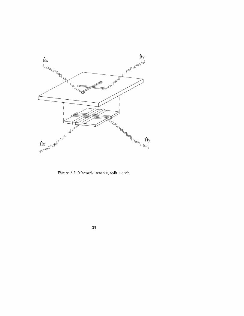
BxBy
HxHy
Figure 2.2: Magnetic sensors, split sketch.
25

HV power supplyLaser + tube l. control
Photo PD load/detector buffer amp B-coils Buffer ADC DSP amps RAM PC H-coils DMA ISA bus EtherX-yoke Current net amps DAC Y-yoke UNIX system AOM RF - XTAL driver osc
Figure 2.3: Block schematic of electric part of measurement system.
190150
140 280 20
20
Test specimen
xz
y
Figure 2.4: The magnetic yoke con�guration. Dimensions in mm.
26
experimenter wants even lower frequencies, the measurement of H-�eld has to be
done with Hall probes, that are not currently used in the setup.
The upper limit is due to the impedance of the feeding coils together with the
magnetic circuit. The impedance increases with frequency and at high frequencies,
the impedance is almost purely inductive. The peak current needed to create the
wanted ux density is constant over the frequencies, and within the range of the
current ampli�er (8 A max). The current ampli�er has a limited output voltage
(about 60 V max), and this voltage will be reached at the upper frequency limit.
The currrent and the upper frequency limit is calculated below.
The reluctance R of the magnetic circuit sets the required current I to achieve the ux density B in the sample. The reluctance for the circuit is the sum of yoke (Ry),air gap (Ra) and sample (Rs ) reluctances. Geometry and materials determine the
reluctance. The air gap between yoke poles and sample can be l0 = 0:1 mm, yokeheight (of midline) is l1 = 140 mm, yoke length (pole gap length) is l2 = 260 mm,
pole widths are w = 20 mm and b = 140 mm and sample sheet thickness can be
t = 0:3 mm. The permeabilities of the yoke and the sample can be set to 5000�0for purposes of estimation. Air permeability is �0. These values give the followingreluctances,
Ry =2l1 + l25000�0wb
= 0:0386=�0 H�1 (2.1)
Ra =2l0
�0wb= 0:143=�0 H
�1 (2.2)
Rs =l2
5000�0wt= 8:67=�0 H
�1 (2.3)
R = Ry +Ra +Rs = 8:85=�0 = 7:0 � 106 H�1 (2.4)
It is seen that the sample reluctance strongly dominates in the example. With 1
mm airgaps and a high permeability sample, the air gap reluctance and sample
reluctance might be of equal magnitude. If a peak ux density B = 1:8 T is wanted
in the sample, a ux � = 1:8bt = 1:8 � 0:14 � 0:0003 = 75:6� Wb should go round
the circuit. The required current in the feeding coils becomes
I =P hi
RN = 1:32 A (2.5)
as the magnetomotoric force is reluctance times ux. N = 400 is the number of
turns of the coils on one yoke in the setup. The current is well below the 8 A max
limit of the current ampli�er.
The current I through the feeding coil inductance L produces a voltage U that
27

reaches Umax at the frequency fmax. The inductance L is
L =
I=
N�
I=
30:2 � 10�31:32
= 22:9 mH (2.6)
from values in the previous paragraph. is the ux linked with the coils. The coil
reactance is X = !L = 7:2 at 50 Hz. The coil resistance is about 2, so the
reactance will be 36 times larger than the resistance at 500 Hz. By neglecting the
resistance, the voltage over the coils will be U = !LI , which gives the maximum
frequency
fmax =Umax
2�LI=
60
2�22:9 � 10�6 � 1:32 = 320 Hz (2.7)
At this frequency, the reactance is 46.
The maximum frequency can be pushed upwards by two methods. The �rst is not
to go to such high peak uxes. This will require a lower current and the frequency
can be increased before hitting the voltage maximum. It can also be seen by the
alternative formula fmax = Umax=2�. This formula also shows that a change
of reluctance (air gap change, material change) won't change the frequency limit.
The only thing that counts is the linked ux, and that normally has to be set to
achieve the wanted ux density. Here one sees the second method to increase the
frequency maximum. By lowering the number of turns of the coils the linked ux
can be decreased and the frequency increased. To keep up the magnetomotoric
force that drives the ux, the current then has to be increased. For the levels in
the previous paragraph, the current can be increased 6 times before reaching the
current maximum of the ampli�er. That allows for a reduction to 67 turns on the
coils with the same magnetomotoric force, same ux and six times lower linked ux.
The maximum frequency is then increased to 1.9 kHz.
It should be noted that the maximum frequencies are for the fundamental of the
excitation. Smaller harmonics can be added. As an example, for the 320 Hz limit
case, a 3.2 kHz current harmonic can be added if it is ten times lower in magnitude
than the fundamental.
2.7 Voltage or current sti� ampli�er
Two control methods have been tested:
Current sti� measurement uses a simple regulator with current sensing of the am-
pli�er that feeds the coils of the yoke. The current on the output can then be made
proportional to the voltage on the input.
28

Voltage sti� measurement uses the raw ampli�er, i.e. the voltage out is proportional
to the voltage in.
The current-sti� ampli�er has the bene�t of being easy to demagnetize with. Har-
monics over the fundamental frequency due to saturation can often be corrected
with the regulator's ampli�cation. The drawback is that the current is not com-
pletely correlated to the magnetic �eld intensity in the sheet due to the air gaps,
saturation and leakage. The air gap is the main source to this phenomenon. In
the extreme case, the coil current will only set up magnetomotoric forces across the
air gaps. Due to ux conservation, the ux density in the material will then be
controlled by the air gap �eld strengths and in turn by the coil current. By lowering
the air gap length, the coil current will control a combination of ux density and
�eld intensity in the material. The ux-current correlation is also the reason for the
experimental fact that circular (Bx; By) is easier to obtain than circular (Hx; Hy)
when performing measurements with rotating magnetic �eld.
The voltage sti� ampli�er has the bene�t of having fewer components. The voltage
being independent of load also corresponds to a more usual situation in applications,
which one might want to simulate in the setup. A problem when measuring uniaxial
B � H curves with the current sti� circuit is that due to the rapid change of Bwith H close to zero, the density of data points can become sparse in that region.
With voltage sti� measurement it is easier to get equidistant points on the ordinate
B. The major drawback with this mode of operation is that it is much harder to
demagnetize samples. The voltage on the output corresponds to the ux derivative
and there can be a constant component of ux present even as the voltage is made
to approach zero.
2.8 B-coils
B coils are used to measure the ux density in the specimen. Either the coils are
wound around a central part of the specimen by the use of holes pierced in the
sample, or the coils are wound around the whole sample.
The ABB program ACE was used to investigate how holes in the sample could
in uence the magnetic �eld. Such a simulation will take care of magnetization
discontinuity on hole edge (equivalent to monopole distribution) and the �eld dis-
tortion arising to lower energy by avoiding the air. The simulation won't take care
of the fact that magnetization will be distributed over domains with continuously
di�erent size and discretely di�erent shape and direction. The holes (as seen by
N�eel) will on that level act as nucleation centers for needle-like domains (with a
transverse to main domain magnetization direction). They will grow under the in-
29
crease of �eld and can act as secondary source for the creation of main rectangular
domains. Thus, the in uence of holes could be larger than seen on simulation.
The continuum simulation showed a completely negligible distortion of homogeneity
of �eld when four 1 mm diameter holes were punched at midpoints of 60 mm sides
of a square, both for isotropic and anisotropic material. The author believes the
result for isotropic, polycrystalline material, but for modern, intensely anisotropic,
textured material the simulations can be doubted. It has been heard that mag-
netostriction is changed a lot by only pressing sharp tips into the sheets of such
material. Such rumours have been taken seriously and the holes have only been
used for B pickup coils when measuring on nonoriented (isotropic) motor iron and
for conventional types of oriented (anisotropic) transformer iron. The superoriented
kinds of SiFe sheets have not been pierced, and coils have been wound around the
whole sample.
In the case for B coil wound around sample, other factors enter: dead magnetic
zone due to cutting of sample and inhomogeneity of �eld strength. The dead zone
is a fraction of a millimeter in width. Inhomogeneity is due to the pole pieces
being 140 mm wide while the sample is recommended to be 305 mm wide. The
recommendation is for the sample to span the pole gap of 280 mm, provide some
area to rest on table, and avoid edge e�ects including dead zone. One might think
that measurement with wide coils would give a good result in the low permeability
direction ( ux spread out along crossing midline) and a poor result in the high
� direction ( ux more concentrated from pole to pole). When experimenting, it
appears that in the low permeability direction, the ux actually tend to enter the
nonactive poles and can cause problems with feeding the magnetic circuit. It is
felt that the strong anisotropy in the sample together with the longitudinal yoke
forms a magnetic circuit that constitutes a kind of bar to transverse magnetization.
Either the ux enters and leaves the same pole without much penetration of the
yoke, or the ux actually circulates the yoke. The last hypothesis is likely when
there is a misalignment of the sample, and as the yoke is laminated and glued,
a transverse enter-leave path is quite inhibited due to the reluctance of the glue
layers. The exact analysis of the problem has been put on hold as the remedy to be
able to make transverse uniaxial measurements is simply to remove the longitudinal
yoke, as it is allowed by the setup. For rotational ux density measurements, no
100% solution is given. As rotation in that case basically only will mean a large
Barkhausen (discontinuous) jump from the longitudinal to the transverse direction,
and it is the nature of that jump that is interesting, the author proposes that the
sample be turned so that the hard (to magnetize) direction is aligned straight pole
to pole. As the B pickup coils still will be wound around the easy and its transverse
direction, information can be collected on how the jump happens by rotating the
excitation in the new con�guration. Geometry gives minimum sample sides of 300
mm for 45 � sample rotation and 385 mm for 30 � rotation.
30

Plate
Coil
1,1
1,2
2,1
2,2
40
30
30
20
10
10
Figure 2.5: One H-coil wound from up to down around a nonmagnetic plate. Hall
probe positions for calibration are marked with circles. Dimensions in mm.
2.9 Calibration of the H-coil
The coils for measurement of H-�eld in the RSST was calibrated by placing them
in the departemental LDJ electromagnet and comparing the results they gave with
measurements made by Gaussmeter and Hall probe.
One have
�0H =1
NA
ZU dt
where N is number of turns and A is the single loop area. The problem is to
determine NA for both directions of the composite H-coil. For each of the two
directions there were four runs with di�erent placements of the Hall probe relative
to the coil. The placements are shown in Fig. 2.9. The directions that the double
H-coil can measure �eld strengths in are called I and II; direction I is marked with
a little bit brown tape on the connecting wire to be able to relate the correct coil
with the calibration data below.
Linear regression gave a standard error for coe�cients less than 0.3 %. The results
31

Position 1,1 1,2 2,1 2,2
NIAI (cm2): 352.47 351.55 349.10 349.95
NIIAII (cm2): 370.12 370.65 368.12 366.56
Table 2.1: Calibration factor as function of calibrating Hall probe position.
varied with the Hall probe placement according to Table 2.1. If the average is taken
one gets
NIAI = 350:8� 2cm2 (2.8)
NIIAII = 368:9� 2cm2 (2.9)
2.10 Measurement table
The measurement table top that supports the interferometer, the yokes and the
sample support is made of black diabase, a kind of granite stone. The table top is
depicted in Fig. A.15 and the whole table is in Fig. A.16.
The table top was drawn, and a proposition from the French �rm Micro Controle for
making the granite construction was received. It was found that their facilities for
treatment were excellent, with high performance drills for making the optic mount
hole picture and proper tools for grinding, why they could obtain a high degree of
atness of the stone surface. Granite was of course chosen by us because of the
absolute necessity of having a platform made out of a electrically non-conducting,
or at least poorly conducting, material to avoid considerable eddy currents, that
would inhibit the production of a high ux density in the specimen, and also make
the control of the �eld in the specimen harder at some of the frequencies we have
in mind. Granite also has a high mass density and a fairly high elastic modulus to
mass density ratio, which will keep deformation mode amplitudes low and at fairly
high frequencies, respectively.
While Micro-Controle had proper tools for machining, it was decided not to order
therefrom because of a high price, the long transportation necessary and the cultural
barrier to design and fault discussions. Sweden has some granite industries so we
consulted the �rm Mikrobas instead. They provided a block of black diabase, said
to be the granite type of highest quality in terms of internal motion, and made a
custom treatment. This treatment consisted of grinding to higher degree of atness,
drilling of optic mount holes and cementing of M6 tapped inserts in these holes.
Geometry of the block was set to the standard thickness of 75 mm and a square
32

width of 1000 mm. The block weight is at a tolerable level, it arrives at 202 kg.
The atness of the stone surface is superb, 55�m tolerance, much higher than
needed in the present application. It can be used as a atness reference for various
mechanical tools.
A drawback with granite is its "ringing" characteristic, high frequencies or impacts
seem to give sustained responses with low damping. Keep silence in the lab room.
2.10.1 Support placement
The choice of area of the block also has some implications to support placement and
method of erection of the setup. It was proven that the weight allowed positioning
with in-house equipment. It would have been better to have tried to reduce the
width to 80 cm, to move the setup through door openings in the mounted state.
Rigid steel supports are currently used, which do not really damp vibrations enter-
ing from the oor. If noise therefrom would be too disturbing (no measurement yet
has had any negative e�ect of it), one can purchase pneumatic dampers, working
with a combination of rubber balloons and mechanical pendulums. There has been
a new product entering the market for vibration isolators recently, that is called
the sub-hertz isolator, which uses a support system passively acting as a spring
with an e�ective negative spring constant, thus counteracting vibrational forces.
The product is very expensive though, and is currently only for light single loads
such as microscopes, that need vertical vibration reduction. The transmission of
vibrations is in this case ten times lower than any other isolator, so performance is
supreme in theory.
2.10.2 Optic component placement
The arms of the interferometer are quite long, and due to the limited area of the
table top, the beam paths have to be folded. The HeNe laser head (from Spectra-
Physics) has a diameter of 45 mm and are 400 mm long, and it is quite desirable
to mount it such that it doesn't extend beyond the edge of the stone. Guiding
equipment is therefore placed before the edge of the silicon-iron sample. It is
believed that symmetry of the setup must be kept, thus leaving the same space
all around the peripheral of the test sheet, in order to be able to �t another laser
head if wanted. Something to consider when choosing size is also that the sample
holder/table should be possible to rotate to be able to measure at about 45� fromthe longitudinal direction to determine the shear in the unrotated system, and this
without tricky beam re ectors. The optic components for guiding reference and
33

measurement beams will be mounted on aluminum rails at some distance to the
yokes in order not to in uence ux picture. The standard mount hole picture on
commercial metal tables dimensioned in the metric system is a matrix with 25 mm
between centers. If the same picture would have been drilled on the granite table,
approximately 1000 holes would have been made. This kind of picture is not needed
since all optic components are mounted on sledges moveable along the rails. The
needed number of holes to �x the rails with some options for di�erent placements
are about twenty.
2.11 Vibration of material
Vibrations due to pulsating magnetic �eld are of three kinds.
� Rigid or bending vibration due to so called reluctance forces on a magnetic
object surrounded by air. The resultant force FR can be calculated with a
Maxwell stress equation
~t =1
2BH ~en (2.10)
~FR =
I~t � d~S (2.11)
where ~t is a traction (force per unit area) vector, and the integration is taken
over a surface enclosing the object, with the surface completely in air, real
or in an imagined in�nitely thin air gap. Maxwell himself regarded similar
traction expressions as valid for the mechanical stress due to magnetization
also within bodies. The modern viewpoint is perhaps that only the integrated
resultant force is valid, but the expression for the traction (force distribution)
on the object surface can also be believed for separate interacting objects.
� Forces on eddy currents induced by the the magnetic �eld. If an oscillating
ux density penetrates a thin sheet obliquely, the normal component can
induce a large eddy current circulating in the plane of the sheet. If such an
eddy current Je exists, the force volume density will be
~f = ~Je � ~Bt + ~Je � ~Bn (2.12)
where Bt is the ux density component parallel to the sheet and Bn is the
normal component. The �rst part of the expression will correspond to a nor-
mal force that might bend or shake. The circulating current picture suggests
that there will be a tilting action when the parallel ux is laminar. The sec-
ond term can be imagined, from the circulating current picture, to set up
34

a compressive stress towards the center of the circulation. A sheet is much
weaker in the lateral direction than in the plane, so a bend is probably more
of a worry than strain. As a thin sheet also will be light, the tilting action
can be suspected to produce a shaky motion.
� Magnetostrictive vibration. Suppose that a core is carrying a ux �. The
magnetostriction is an even function in the ux density, we can use B2 = P�as a model when reasoning, where B2 can be thought of as a magnetic stress,
P as a sti�ness modulus and � as the magnetostrictive strain. If � is given in
the core, as is often the case for voltage sti� excitations, there are a few ways
to reduce the vibration amplitude:
{ Increase the area of the core to decrease B. (More core material, cost
increases).
{ Use material with higher P . (Better core material, cost increases).
{ Passively damp the transmission of vibration with sound insulation.
(Polyurethane, maybe not so costly).
{ Actively counteract with actuators out of phase with the vibration. (Dif-
�cult and risky).
{ Apply tensile stress to the material when there is a positive stress sensi-
tivity �P�� of the material.
Attempts to dampen the vibration by clamping the material perpendicularly
to the direction of vibration is not guaranteed to be successful. The magnetic
action that shows as magnetostriction is very strong, and can easily make
the clamping device vibrate too, perhaps leading to a worse transmission of
sound. There might be a positive e�ect from a lateral stress dependency if
the clamping device suits the nature of the problem.
2.12 Digital control issues
If a digital feedback control would be employed, the nature of the sample material
would drastically in uence the feedback algorithm.
The two industrially used types of silicon-iron alloys are being investigated. The
non-oriented sheets used in motor applications pose less demand on the control
program, since there is no strong macroscopic anisotropy present. In a rotational
�eld case, the computer only has to store hysteretic lag information along with
a direction cosine lookup table for the ampli�er outputs to adequately steer the
controlled �eld vector. Grain-oriented sheets (in the case of a circularly rotating
ux density) will also require an additional table to additionally enlarge the applied
35

transverse component when the �eld direction is moved into the di�cult region
around the magnetically hard axis, which is at 54:7� from the rolling direction of
the sheet.
In the case of experiments when only one cycle is measured, past history has to
be cleared by saturating the material or magnetically cycle it. Magnetic cycling
with the amplitude continuously decreasing from saturation to zero is also called
demagnetization. Simple saturation can be used for really large major loop mea-
surements, such that the �rst loop guarantees saturation and the second loop is
measured. Most measurements are not with that hard saturation, and a demagne-
tization wave is sent prior to measurement.
When conducting basic research, not much is known to the experimenter when a
new sample is taken to be measured. The �rst measurements become an explo-
ration of the material and are done with no or very primitive control. Based on
knowledge gained from the exploration, one can be ready to take control. The
simplest is to manually change the input signal to better achieve an intended �eld
signal. Automatic control using hysteresis models and parameters from initial mea-
surements are possible, but there has not been time to code a suitable algorithm
for the acquisition board. If someone would like to try it, he or she should be aware
of the existence of delays from board input to memory input and from executed
output to board output due to the use of delta-sigma analog to digital and digi-
tal to analog converters. Delta-sigma converters use a bitstream technique with a
control/comparison loop to convert analog levels to digital numbers or vice versa.
The control loop introduces a time delay between the sampling of the analog level
and the output of a number.
2.13 Strain measurement by interferometry
The setup is able to retrieve strain information from a laser interferometer. Three
pairs of mirrors glued to the surface of the sample are subjected to internal relative
translation as the magnetization is altered in the area of measurement. As a result,
the laser beam is re ected by the target pair of mirrors whose relative displacement
shows as a phase shift between measurement beam and reference beam after those
two beams have been recombined. This timevarying phase shift can also be seen as
a Doppler-shift in frequency due to the di�erence velocity of the mirrors. One of the
beams can be frequency-shifted (or frequency split which corresponds to intensity
modulation) so that a phase carrier (a "running" phase) is superposed on the object-
caused phase shift. This carrier makes the detection of sign of strain change possible.
It can also be used to avoid low-frequency noise. The detector of the phase shift is
a photodiode. Its output current (or voltage over a load resistor) is proportional to
36

the light intensity which in turn is proportional to the cosine of the phase shift. The
output voltage is sampled by the digital acquisition board. The voltage waveform is
then demodulated on the host PC, to arrive at the desired displacement from which
the local strain component is calculated. The demodulation code could be moved
to the board, but as it depends on the calibration with a known whole wavelength
displacement (either from the true object or an arti�cial disturbance), it requires
some operator validation and iteration that is most conveniently carried out on the
host.
There is sensitivity to the environment. Tramping on the oor, light knocking on the
table and loud voices in the lab room (4x3 m) are clearly seen in the interferometer
signal.
2.14 Stress in uence, frame e�ect
In the above, the handling of the B, H and � state variables have been presented.
The fourth variable � must be adequately analyzed in order to well de�ne the
measurement conditions. The less magnetized outer regions of the sample will act
as a frame around the central region, slightly resisting the strain of the central
region. Thus, there will be an elastic component of the strain tending to reduce or
smooth out strain arising from magnetostriction. This phenomenon is analyzed in
detail elsewhere in this text, with the conclusion that about 10% can di�er between
true magnetostriction and measured strain.
2.15 Yoke design
Field calculations have also been extensively used for the calculation of general setup
performance. The yokes constituting the magnetic circuits are laminated to provide
�eld homogeneity in the sample. Also an airgap between the sheet under test and
the end of the lamination is introduced. This increases the homogeneity and makes
the magnetic reluctance force more well- behaved, compared to letting the sample
rest directly on the ends of the yokes. The signi�cant reluctance introduced by the
air gap makes full saturation harder to achieve. The reluctance force between the
sheet and the yokes are carefully balanced out by adjusting the air gap to the upper
air of yokes, which are separately �xed to the vibration damped measurement table.
In fact, to properly balance the force one has to have coils on the upper pair of yokes
also. This is due to the fact that a large part of the total ux deviates from the yoke
loop in the magnetic circuit into the sheet under test, even though the crossectional
37

area of this sheet is very small. As the force is proportional to the square of the
ux, there would be problems to balance this deviation only by adjusting the air
gap length. It is also probably only to an advantage to have symmetrical poles with
coils wound close to the edges of the yokes from a leakage and drive current point
of view.
Finite element calculations have also been made to determine the area of homoge-
neous B, � and � �elds for a variety of excitations. This area is suitable for sensor
positioning. The current setup has 24 cm of inner spacing between poles, which
are 14 cm wide and 2 cm thick each. This produces an area of homogeneity which
is 10x10 cm square. It might be considered a good compromise between easy han-
dling of reasonably light equipment and bene�ts of having a large distance between
re ectors when it comes to resolving the strain signal for very low magnetostrictive
sheet types. On the other hand, for these sheet qualities it is possible to make a
pure uniaxial measurement with a mirror spacing of 20 cm, as the homogeneity
region is larger for this simple type of excitation.
2.16 Magnetic sensor design
The fundamental concept of recording of all state variables re ects itself on the sen-
sor equipment. Induction coils for the measurement of the ux density are made
as one loop of 0.1 mm diameter isolated copper conductors thread through drilled
holes in the specimen. Again, �nite element calculations have been applied to in-
vestigate the performance. It is seen that the ux enclosed is very little changed
by the introduction of 1 mm holes compared to the ideal homogeneous permeabil-
ity case. What is worse is that the holes will serve as nuclei for domain growth at
magnetization reversal, thus violating the basic assumption of a homogeneous mag-
netization characteristic of the measurement area. One might therefore consider to
use a needle technique, in which two pairs of needles are brought in contact with
the sheet to form a closed loop as the induced current will pass through the sheet
twice. The low conductivity of the sheet, together with the one loop condition, will
make the signal to noise ratio very poor, though. With a good sensor ampli�er
and DSP noise reduction capabilities, it might be considered as a check of Weiss
domain conditions.
The induced current in a sensor copper loop will be in the order of microvolts. To
be able to feed the signal onto the A/D-board, it has to be ampli�ed 100 dB. This
signal level, as the ampli�ers are placed close to the sensors on the measurement
table, will also protect the signal from environmental noise.
The magnetic �eld intensity is raised with a factor of approx. two in the holes
38

compared to the homogeneous case. While the ux essentially avoids the holes
completely, the H-�eld will broaden its peaks due to the tangential continuity and
a�ect the region between the holes slightly. Thus, the Rogowski coils used to
measure the H-�eld has to be geometrically somewhat shorter than the distance
between holes. The 1 mm thick Rogowski coils are placed directly tangential to
the specimen surface, in order to use the continuity of the �eld intensity and the
simple relation B = �0H in air to measure the magnetic �eld intensity. It has
to be realized though, that the H-�eld is not completely uniform in the direction
inwardly normal to the sheet. To get the average �eld, one is forced to rely on
simulations to calculate a uniformity factor. Of course, this factor is a�ected by
eddy currents and the so called anomaly occurring when eddy currents are induced
in ferromagnetic materials. There is still little quantitative knowledge about this
e�ect so simulations have to be performed in an ideal vs. worst case manner.
2.17 Temperature drift
Another state variable to consider is temperature. During a long measurement, it
is possible that a temperature drift in the order of a degree will occur. The best
situation is then to record, albeit not very densely in time, the specimen tempera-
ture along with the rest of the variables. When interferometric measurements are
performed, it is also desirable to measure the temperature of the air, as the index of
refraction of air is somewhat dependent upon it. The specimen temperature can be
measured by gluing an NTC- resistor to its surface. A drift of 1 K will elongate 10
cm of silicon-iron with a nanometer. The in uence of such a drift on magnetization
is very low. Classical eddy currents at 50 Hz uniaxially alternating magnetization
will give rise to approximately 20 mK of heating due to loss.
The sources of temperature drift are the power ampli�ers in the room, power sup-
plies to control and measurement hardware and the excitation coils. If the excitation
coils are overheated in an experiment with high current during a too long time, a
slight smell can be felt from the hot insulating lacquer on the coil wires.
2.18 Signal conditioning and Nyquist limit
Another source of drift, let alone of a di�erent kind, are the analog measurement
signal ampli�ers. These are realized by the use of low noise TL072 operational IC:s
and high-quality precision passive components in feedback and signal paths. The
main issue regarding these ampli�ers are that they add a (constant) o�set volt-
39

age to the ampli�ed signal. These o�sets are easiest compensated for by digital
postprocessing of the sampled signals. A routine for such digital compensation is
needed anyway, since the integrated ux signals have to be o�set compensated also.
Both before-integration and after-integration o�set compensation are done by the
graph program. Two options can be chosen from when starting the graph pro-
gram: -mean and -median. The -mean option adds a constant to the signals so that
the time averages are set to zero. This is the usual choice for periodic, symmetric
signals. Also damped oscillatory signals often turns out to be well compensated by
this method. The -median option sets the median of the peak and bottom values to
zero. That option can be used for signals that saturate the material both at peak
and bottom values, but are otherwise nonsymmetric. Both options operate at both
the before-integration and after-integration steps.
The A/D-board comes without so called signal conditioning circuitry and one has to
take that into account also. The topics that typically arise are those of anti-aliasing
and sample-and-hold during A/D-conversion. When there is a non-negligible energy
in the high-frequency end of the signal spectra, as seen in the magnetostriction
measurements, aliasing must be avoided by introducing a passive linear-phase Bessel
�lter of enough order to cancel the frequencies above the Nyquist rate, a �lter that
can be tricky to build, especially if the order has to exceed two. The Nyquist
frequency is 26 kHz for the DT3818 board when the sample frequency is set to the
maximum (52 kHz). This range will well cover the magnetic frequencies for normal
experiments. The yokes cannot be fed with frequencies much above a kilohertz (see
section on frequency limits), and with a kilohertz fundamental the board still allows
for twentyfour harmonics. There is a complication here, due to the fact that the
ux density time signal is often at for a relatively long time (material is saturated)
and then changes rapidly as the ux density passes the steep part of the hysteresis
curve. To catch the steep parts of ux changes, which corresponds to spikes in the
voltage that is really sampled by the ADC:s, the sample frequency cannot be set
too low.
The 26 kHz Nyquist frequency is more of a limitation for interferometric signals.
A �fty hertz magnetic fundamental yields a hundred hertz magnetostriction fun-
damental that will be multiplied by the number of temporal bright fringes each
strain cycle produces. For a large magnetostriction signal, something like �fteen
fringes can be produced from bottom to peak strain. That results in a three kilo-
hertz interferometric signal, when the fringes are spaced equally in the temporal
dimension. In that case, eight harmonics can be treated, which still is a fair num-
ber. The complication with rapid changes in ux density will also be seen in the
interferometric signal, the fringes will be crowded around the rises and falls of ux.
The sample frequency is most often set to the maximum 52 kHz for these measure-
ments. To spread out the fringes in time, the peak value of the excitation can be
lowered (simply by adjusting a gain option to the measurement program) so that
40

the material doesn't go so hard into saturation. If hard saturation is wanted, an
exciting waveform can be created that passes the steep part of the hysteresis curve
more slowly.
The A/D-converters do have to be fed by a constant signal during the time of the
conversion. To provide this piecewise constant signal, a sample and hold circuit,
in principle a solid state implementation of a switching transistor and a large ca-
pacitor, is provided built into the conversion circuits. The switch trigger signal is
available at the A/D-board. Conversion circuitry uses the now highly popular bit-
stream technique which, although avoiding signi�cant bit errors, could introduce
problems connected to jitter in timing signals, as the clock frequency is heavily
increased compared to old-fashioned parallel converters. No such problems have
been observed. The resolution is 16-bits, which means that the data is amplitude
resolved in steps of 1/65536. When frequency analysis then is performed on stored
raw data, one has to conceive the semi-white digitizing noise thus introduced. For
ordinary measurements, this does not cause any problem.
2.19 Signal bu�ering
There are eight AD converters and two DA converters sampling and working in
parallel and they store and fetch data from two bu�er queues (streams). Problems
can easily occur with these streams. If the queue handling is inadequately treated
by the program, bu�er �ll ups and emptying can happen before new bu�ers are
placed in the queue (overruns). This is a bit tricky when the DA stream continu-
ously should receive new bu�ers to produce signals with very long durations, with
simultaneuous AD input bu�er treatment. The library functions supplied with the
board (SPOX functions) that handle bu�er gets and bu�er puts don't return until
a �lled or emptied bu�er is available in the queue. The queues normally consist
of three bu�ers each of equal length, and when choosing all eight AD inputs the
in queue will �ll up much quicker than the out queue is emptied. This causes a
risk of in queue overrun while the main program waits for an out bu�er to become
emptied to switch in a new bu�er to output. The program dtacq can handle this
situation by calling the right number of in bu�er gets for one or two out bu�er
puts, and not initializing the out queue completely to provide room for out bu�er
switch-in without main program stalling.
The user has to be concerned about how many ADC:s he/she will use. If a DA
waveform has 1024 time points, the bu�er length might be selected to 1024 points
also. If two DA:s are operated in parallel, a bu�er will be �lled with 512 points from
each channel (channel samples are interleaved). That is �ne, the program will then
only use two bu�ers to make a complete signal frame. The bu�er length will hold
41

also for the AD side, meaning that the number of AD:s cannot be chosen arbitrarily.
Eight AD:s (the most common choice) means that in the current example, 128
samples from each AD is placed in a bu�er. That works. If �ve AD:s would be
chosen, they wouldn't �ll up a bu�er evenly. The last free space in a bu�er would
be �lled up by three AD:s and two AD:s would have to try to place their samples
in the next bu�er. It won't work. The board cannot handle this uneven situation,
and will lose data. Not just a few samples are lost but complete bu�ers. If this
happens by mistake, the acquired signals will contain strange jumps or spikes, that
are characteristic of this problem. The simplest rule is thus to use a 1024 sample
bu�er length (for reasons below) and 1, 2, 4 or 8 ADC:s.
The bu�er length also has to be set by the user with the -bu en option. The
natural length for the board is a multiple of 512 samples, with a minimum of 1024.
Overly long bu�ers will cause board memory �ll ups. For example, 10240 samples
per bu�er gives 61440 samples of total stream bu�er memory (2x3x10240). Each
sample is a board CPU word which is two octets (PC bytes), which means that 120
kbyte of board memory is then used up. The total board memory is 256 kbyte, so
too little room is available for SPOX functions, the main acquisition program and
data stored for loading/unloading stream bu�ers. The method for long signals is
to segment the signal with the -bufs option to the program. This option tells the
program the ratio of the number of time points of the complete signal to the bu�er
length. For a single channel signal, it is the number of bu�ers it would �ll up on its
own. The fundamental bu�er length can then be kept short at 1024 samples (the
usual number) which only gives 12 kbyte of stream bu�er space. By creating the
output signals with the pcgen program on the PC the lengths are easily adapted
to a multiple of 1024. If the use of this program is impossible, the signals can be
zeropadded to achieve a suitable length.
Two other arguments have to be given to the dtacq program, but no risks are asso-
ciated with these. The �rst is the number of signal frame repetitions to be put out.
By using large numbers, very long signals can be generated by the DA converters.
This is good for cases where manual observation, adjustment and experimentation
is necessary. The second option is the number of repetitions before the actual
measurement frame. Using a frame or two in front of the �nally stored frame is a
practice to get rid of transients, when these are unwanted. The unmeasured frames
are called delay frames. Larger numbers of delay frames are useful when something
has to be manually veri�ed or in uenced precisely before the actual measurement.
All options to the dtacq program can be listed by invoking the program without
any argument.
42

2.20 Measurement coil misalignments
Systematic errors in measurements can occur when the magnetic �eld sensors are
not lined up strictly in parallel with the preferred and the transverse directions
of the silicon-iron sheet. This has been foreseen, and it can be compensated by
two methods. The �rst is that the H-sensors are mounted on a detachable board
so that the angle position of these is easy to change. To test that the sensors are
accurately lined up, one can make use of the magnetic �eld trace re ection property
of the sheet. This means, that if the trajectories of the magnetic �eld in the ~Band ~H-spaces are re ected in the principal directions of the sheet, the same trace
shape is obtained. By tracking a quasi-DC measurement, one is therefore in the
position to determine the misalignment of the sensors by mathematically adjusting
the deviation angles with coordinate transformation, so that the re ection property
is obtained. Of course, this is simpli�ed by very de�nitely �xing the relative angle
between the Rogowski coils to 90 degrees. This test method might also be put in use
to postprocess already measured, somewhat alignment erroneous, data. To be able
to do this, one must anticipate the possibility and remember to trace out the �eld
twice, in 180 degrees opposition, and activating a complete history clearing there
in between. The measurement pair is then stored in parallel and the misalignment
angle is calculated from the angle deviation in expected �eld and measured �eld.
There is only a need for a single trace-out if the inter-coil angle is 90 degrees �xed.
Misalignment of the B-coils can only be compensated by the software method when
these are wound through drilled holes in the sample.
2.21 Using the measurement system
2.21.1 Magnetic measurements
Hrd, Htd, Brd and Btd can be measured simultaneously during uniaxially alternat-
ing H or rotating H - excitations. For a non-oriented material such as DK66 this is
easily done. For strongly oriented materials such as ZDKH there might be problems
to rotate the magnetization vector out of the rolling direction. When exciting the
transversal yoke in such a case, there could be a coupling between the yokes due to
the sheet which is harmful to �eld homogeneity and possibility of achieving a high
peak ux. When only wanting transversal data, it is possible to detach a yoke and
make a single yoke measurement.
Demagnetization of the RD direction of oriented samples can be hard, due to the
relatively high remanent ux density that occurs at zero �eld strength. An alter-
43

native is to demagnetize the sample in the transversal direction before the rolling
direction.
2.21.2 Peak ux
How does one get a higher B in rolling or transverse direction? It can quite easily
be achieved by increasing the gains given to the data acquisition board for output
signals. The Techron current ampli�er can put 8 amps max into the driving coils,
and with 200 turns of each yoke coil, there is plenty of excitation available. Limiting
factors are leakage (since the sheet under test is very thin), yoke cross coupling
(noticeable for superoriented samples), and high reactance of coils especially at
higher frequency due to a large number of turns (inductance).
2.21.3 Measurement procedure
The procedure for making a measurement is now described. The operator should
make the interferometer alignment on a dead (non-excited) object �rst, then place
him/herself behind the measurement system PC. The whole sequence of program
invocations and data archiving is automated by a DOS batch program, calledmeas.
The user can interactively select yoke con�guration and sample alignment (direc-
tion). Two or three excitations are then on sequence, the �rst with a very low
fundamental frequency for the operator to be able to view the interference on the
paper screen with the eye. If approved, the photodetector is inserted in its holder
and the interference can be checked on an oscilloscope, by using the second excita-
tion that has a higher frequency. At this stage a �ne tuning of the corner mirror
is possible to improve temporal fringe visibility. The �nal measurement is done in
the third step of the sequence.
The programs that are called by the master batch program are pcgen for signal
generation, exec3801 for downloading the data acquisition program dtacq to the
DT3818 board, and a large program graph for post processing, interactive viewing,
selecting and scrolling of channels to save or plot. Options to the dtacq program
has been covered in section 2.19, and these should be set at the beginning of the
meas batch script.
Viewing with graph is basically done in two modes, channel versus time or channel
versus channel (hysteresis graph). Two y-axes are present, so a maximum of three
channels can be on screen simultaneously. To change channel on an axis and to
adjust zero position (scroll), tic mark increment (scale) and dominating scaling
exponent, the numeric keypad is used. It is sectioned into rows for operation type
44

and into columns for axis. By pressing the key in the matrix corresponding to the
axis-operation wanted and then pressing the + or - key while keeping the other
key down, the change is commanded. While it might sound a little tricky when
described, it feels very natural when actually using the two-�nger commands. Most
convenient is to place the thumb over the matrix and the index �nger over the plus
and minus keys. Some clari�cation of the matrix is appropriate: 1,2,3 changes
channel (1 changes the channel on the left y axis, 2 the channel on the x axis and 3
the channel on the right y axis), 4,5,6 scrolls the channel along corresponding axis,
7,8,9 scales corresponding channel, NumLock,/,* changes exponent. Don't bother
to learn it by heart, a help line is always on screen for you to remember, and it will
soon stick to your hand.
A little speciality is when no channel is on the x axis, which make the graphs to
be drawn against time or point index number. When scrolling the x-position in
such a case, scrolling will be faster (coarser) so that the signal can be inspected
in detail. Data points can be marked and unmarked by pressing a single key.
Single keystroke commands are available for printing the viewed graph directly in
Postscript on printer or �le, saving the viewed channels in ASCII column format,
to FTP a �le to a UNIX host, to get signature (RMS, mean value etc) information,
etc. The key commands available for the screen present can be read out from a
help line.
Postprocessing to be done on signals is commanded by label substrings (extensions).
Labelling has to be done to make the channels identi�able for the operator. By
using these extensions to the labels, extra key commands or options are avoided.
The extension "dot" for example, marks a channel as being the time derivative of
something, and that something will be formed by integration of the dot signal, and
stored as a separate signal. The extension "mod" marks a modulated signal, that
is demodulated and stored by the program. The batch program uses dot on pickup
coil signals to get the uxes, and mod on the photodetector signal to get the strain
as function of time.
A number of options can be given to graph program. In fact the command line will
be long as labels are also given as arguments. DOS has a limit of 127 characters
on the command line so a possibility for using option �les has been programmed as
a workaround. The system user won't have to bother about these �les since they
are created by the master batch program, but the existence of them is necessary
knowledge. Options to graph can be listed just by typing graph without any
argument. There we can see how scale factors (multipliers) are given, that two
methods for integration constant determination are present (-mean or -median to
set the associated property to zero), that a power density time signal (the mean
value of which is loss) can be calculated out of B and H signals, and that eddy
current caused error on the H signal can be compensated from the B signal.
45

Chapter 3
Interferometer
3.1 Introduction
The measurement of magnetostrictive strain is a di�cult experimental problem.
The strain information is retrieved by a non-contact homodyne HeNe laser interfer-
ometer. An overview of the interferometer can be seen in Fig.3.1, and a photograph
can be seen in Fig. 3.2.
The strain information is retrieved by a single non-contact interferometer, which
illuminates a pair of sample micro prisms that senses the elongation of a 70 mm ele-
ment. The Mach-Zender beam path type used simpli�es sample re ector placement
but makes beam alignment more di�cult as there are more degrees of freedom in the
setup. That there is a pair of re ectors for all three strain measurement directions
makes one assured that displacement recorded is relative. The laser is an intensity
stabilized HeNe laser (�=633 nm) that can be switched into frequency stabilized
mode if desired. The acousto-optical modulator (AOM) can facilitate intensity
level alteration when the interferometer is operated in homodyne mode, and can
impose a carrier on the temporal interference pattern to operate the interferometer
in heterodyne mode.
The sample test bed with feeding yokes is possible to rotate on a Te on-glass-�ber
weave, so strain components can be measured in turn while preserving the same
excitation.
46

Figure 3.1: Overview of interferometer
47

Figure 3.2: Actual IFM setup
3.2 Homodyne interferometry
The intensity of the combined beam at the photodetector is I / (E1 +E2)2 where
E2 / cos(!2t) is reference beam �eld strength and measurement beam electric
�eld strength is E1 / cos(!1t + !) . ! is the principal modulation of frequency
caused by variation �L of the measurement optical path as sample re ectors (micro
prisms) move relative to each other. Some algebra gives I = I12 + I0 where I12 /cos(') is a phase modulated interference contribution ( _' = !) and I0 is a constantbackground. Phase demodulation ' = acos(I12=I12) and scaling gives strain � =�xl
=�L=2l
='�=22�l
where �x is relative micro prism displacement, l is (initial)micro prism spacing and � is beam wavelength. Intensity of the combined beam is
sensed as proportional current Ipd through the photodetector diode. Fractions of a
wavelength are possible to resolve when a calibration measurement is done with at
least one guaranteed (and manually eye-proven) complete fringe (i.e. �L > �) froma perturbation of the optical path before the actual measurement. Fractions down
to 1=100 are expected to be possible with initial phase shift precautions noted
below, correct prism mounting insensitive to sample sheet bending at high peak
ux densities and avoiding of phase uctuations (due to air ow, subsonic house
vibration etc.).
48

3.3 Heterodyne interferometry
In the interferometer lab, there is an acousto optic modulator (AOM) that can
be used to operate the interferometer in heterodyne mode. The AOM imposes a
carrier frequency on the intensity signal (which can also be seen as a frequency shift
between the recombining beams) which results in bene�ts discussed below. What is
lacking to be able to try the mode is a rewrite of the demodulating code to handle
the carrier (phase or AM demodulation depending on placement and feeding of the
AOM). An alternative is to set an analogue demodulator (built for AM, also in the
lab) in operation.
With the acousto optic modulator (AOM) operating before the �rst beam splitter
one can write I / (a(t)E1 + a(t)E2)2 / I12 + I0 where a(t) / cos(!ct) is an oscil-
lating intensity modulation imposed by the AOM. This will yield a phase carrier
'c = !ct in the interferometric part I12 � cos('+'c). The phase carrier will basi-cally move the principal signal spectrum up to higher frequencies and it is possible
to avoid LF noise (1/f-noise) that can be a problem for low amplitude strain signals.
Another advantage is the fact that the phase carrier makes is possible to distin-
guish between elongation (phase retardation) and contraction (phase advancement)
around the carrier, without need to resort to old contact measurements or theoret-
ical results. For small strains �L << � (and with initial phase shift adjusted to
�=2 by the use of, e.g, a wave retarding plate in the reference beam path), I12 canbe linearized to give an amplitude modulated photodetector signal. This is simpler
to demodulate (with analog equipment) than a weak phase modulated signal. In
the presence of digital signal processing capabilities, it is probably easier and more
accurate to receive the complete HF-signal, reduce noise by ensemble averaging
and phase demodulate. The upper limit of high frequency is set by the Nyquist
frequency of the data sampling unit (26 kHz). The carrier can be fabricated by
using one channel of the DT data acquisition board for example, and will then be
highly stable. The phase carrier is sent to the RF driver and serves to modulate
the 80 MHz carrier (of the driver) that supplies the AOM crystal with power.
An alternative to make the carrier is to use a crystal controlled oscillator, but the
frequency is then only changeable with frequency ( ip- op) dividers or by manually
swapping the crystal for another with a di�erent resonance frequency.
3.4 Interferometer alignment
As with all interferometers, a big practical issue is how to align the reference and
measurement beams so that recombination of these will lead to an interference
49

as visible as possible. The ideal beam path is never attained in practice, since
the measurement beam has to be somewhat varied in height and angle to strike
the measurement object re ectors correctly. This object adjustment is done �rst,
followed by a beam parallelity adjustment. To succeed, the use of simple tools has
been su�cient. The tools needed are a mirror, iron at plates with punched holes,
and a glass plate. All have been cut to �t between the stabilizing mounting rods
in the setup. The rods run parallel to the beam path on top of the rails that carry
all optic components, so they provide a reference for alignment.
The object adjustment consists of object re ector incident angle correction and
spot height correction. Angle can be adjusted by rotating the sample support table
(including the yokes) on the te on weave that sticks on to the granite table. Due
to the low friction, this rotation is easily managed, even though the yokes weigh
about ten kilograms. Height of spots on object re ectors can be corrected by slightly
changing the elevation angle of launched beams by rotating the beam splitter. The
elevation angle of the reference beam should be coadjusted (by rotating the corner
prism) so that on the receiving side, the spot height of the measurement beam on
the beam combiner1 is the same as the height of the reference beam on the corner
mirror. Control of height at the receiving side can be done with two punched plates,
that have the distance from rail or carriage to punched hole equal to the distance
to the mechanical center of the beam guiding system. Another method, probably
more convenient when the operator adjusts sitting behind the receiving side, is to
check height above sample table with a glass plate or a plastic ruler. Position on
horizon is adjusted by moving the carriages with the combiner and the mirror as
passengers on the rail of the receiving side. Check of this position can be done with
a punched plate close after the receiving components.
Interference is possible when beams are parallel to each other. Visibility of fringes
becomes higher when the spots overlap well, but overlap is not as crucial as paral-
lelity. Laser spots have to be fairly well centered on the photodiode of the photode-
tector, which is �xed at the mechanical center. Parallelizing the beams incident
on the diode is done one beam at a time, with the rods as reference. One beam is
blocked (with a free mounting plate on the sample bed for example) while the free
mirror is put in place of the photodetector. An extra mounting plate is ready there
to press on to the mirror and make it perpendicular to the rods. The misalign-
ment of the incoming beam can then be monitored by sticking the glass plate into
the paths and watching the di�erence of spot position of the incoming beam and
its mirror-re ected companion. The misalignment of the measurement beam can
then be considerably reduced by rotating the tilt table on which the combiner is
mounted. The reference beam is angle adjusted by turning the corner mirror. After
1A combiner is a beam splitter with two incident beams perpendicular to each other. Half ofthe incident beams will pass straight through the combiner, and half will be de ected by 90�. Onestraight passing part and one de ected part will make up a recombined beam.
50

removing the free help mirror and inserting a 15 mm focal length lens in its place,
it should be possible to see spatial interference fringes on a screen raised somewhere
behind the end of the rail. The aim is to get a single spatial fringe on the screen.
The best adjustment screws are on the receiving mirror, it is a good choice for the
last �ne tuning. The �nal state of alignment is viewed by the single black or red
fringe on the screen. Dynamic interference (oscillation between black and red) can
be tested by knocking on the diabase table, or touching/pressing inwardly on the
�ne adjustment screw of the corner mirror.
As stated above, parallelism is most important and the operator should put down
e�ort on that property. A side e�ect occurring when making the beams very parallel
to the mechanical center is that re ections from glass surfaces will travel backwards
into the aperture of the laser. Such retrore ections will make the laser unstable,
a condition that is recognized by an audible signal from a relay switching on and
o� in the control and power supply unit of the laser. To avoid this condition, it
is best to slightly misalign the combining beams with the mechanical center. The
re ections from the help mirror in place of the photodetecor should produce spots
on the support of the last object re ector. Then one is certain that retro-re ections
doesn't travel back into the laser.
Due to the relative sparsity of degrees of freedom in the setup, the adjustments
are slightly dependent on each other. Some iteration of the above procedure might
therefore be required to achieve good interference. The steps that are simple to
iterate are elevation change, carriage postion change and tilt table rotation change.
If needed, the height on the launching side can be changed by inserting or removing
thin spacers that are stuck between the laser head in its mount. When no big
change is involved, the time to perform alignment is likely to be within half an
hour, perhaps ten minutes for a trained operator.
3.5 Doppler e�ect
The Doppler e�ect is the dependency of re ected beam frequency to the velocity
of motion of the re ector and the frequency of the incident beam. This e�ect
is the time derivative view of the phase retardation description mostly used in
interferometry. Since the Doppler view is directly connected with the speed of the
measured object, it is used in velocimetry of e.g. uid ow. If the re ector speed
is v, positive in the ray direction of the incident beam, the frequency at a point
on the re ector will be !s = 2�(c � v)=�i, where c is the speed of light and �i isincident beam wavelength. The re ected wave will have a frequency on the re ector
of 2�(c+ v)=�r . From the equality of frequency of the two beams as measured on
51

the re ector, one arrives at
�r�i
=1 + v=c
1� v=c� 1 + 2v=c (3.1)
where the last approximation holds for small re ector velocities in comparison to the
light speed, an assumption that was understood from the beginning. The frequency
received by a stationary receiver is given by the reciprocal of the above equation,
!r � !i(1� 2v=c) (3.2)
.
3.6 Motion of measurement table
To have a thick table is good, since it reduces amplitude of modes that inject noise
in the relative position of sample and reference re ectors. Modes are energized
by ambient vibrations of the house and the humans in the house. Particularly,
rotating converters in the cellar, walking in the lab room, cooling fans and hard
drives to computers and human speech contribute to noise. Direct knocks on the
measurement table give a ringing signal characteristic of granite, from which the
table is made of. It can be concluded that damping of the material is poor, but it
is compensated by a high mass density.
It is in order to go through the possible vibration modes and give some quantitative
characteristics of the table in question.
The isotropic Hookes law can be written �ni = C�ni; i =1G�i, where G is the
shear modulus and C is the compliance matrix for normal strains,
C =
24 1
Y� �Y
� �Y
� �Y
1Y
� �Y
� �Y
� �Y
1Y
35 (3.3)
The elasticity modulus Y is measured at uniaxial stress conditions. The inverse of
the compliance matrix is the sti�ness (or elasticity) matrix E,
E =Y
(1 + �)(1� 2�)
24 1� � � �
� 1� � �� � 1� �
35 (3.4)
For example, the elasticity coe�cient E11 should be used when uniaxial strain
is present. By multiplying the scalar factor with the elasticity coe�cients the
52

o�-diagonal entries become the Lame constant � = Y �=(1 + �)(1 � 2�). The
constant describes the tension needed to counteract transversal contraction from
an orthogonal stress and keep a given stress in the former direction. It is also
noteworthy that the on-diagonal elasticity entry is not equal to Y , but �(1� �)=�,a result from the de�nition of the elastic modulus as the sti�ness under uniaxial
stress conditions. When isotropic, the material should respond the same to every
uniaxial tension, regardless of its direction. This property gives a constraint on the
shear modulus, it must be equal to Y=2(1 + �) which is in turn equal to �=2, with� being the second Lame constant.
The equations of motion for a continuum are
@x�x + @y�yx + @z�zx = �@2t u (3.5)
cycl:2 (3.6)
cycl: (3.7)
(3.8)
By expressing the terms with the isotropic Hookes law one gets
@x�x = E0(1� �)@x�x +E0�@x�y +E0�@x�z (3.9)
@y�yx = @yG yx (3.10)
@z�zx = @zG zx (3.11)
and by inserting the de�nitions of strain one obtain
@x�x = E0(1� �)@2xu+E0�@x@yv +E0�@x@zw (3.12)
@y�yx = G@2yu+G@y@xv (3.13)
@z�zx = G@2zu+G@z@xw (3.14)
where E0 is Y=(1 + �)(1� 2�).
By changing the order of di�erentiation, completing the terms to get a derivative
of the dilatation r � ~u, and using the formula for the isotropic shear modulus, the
sum of terms making up the left hand side can be written and equated as
Gr2~u+ (E0� +G)@xr � ~u = �@2t u (3.15)
cycl: (3.16)
cycl: (3.17)
2The cycl. symbol stands for an equation that is gotten by cyclical permutation of the indicesin the equation right above it. Examples of such permutations are @x ! @y, �x ! �y and�yx ! �zy.
53

This equation system can be solved with the dilatation as the primary variable. By
taking the divergence of both sides of the system, we get
(E0� + 2G)r2r � ~u = �@2tr � ~u (3.18)
This is a scalar equation in r�~u. The factor E0�+2G is equal to the diagonal entry,
say E11 of the elasticity matrix. A plane wave solution has the dispersion relationE11
�(j~k)2 = (�j!)2, which gives the wave speed cP = !
k=q
E11
�. The index P to
the speed originates from the fact that dilatation is caused by an hydro-like pressure
acting on elements of the continuum.
At zero dilatation everywhere, there can still be waves of pure shear travelling.
Inserting r � ~u = 0 in the wave equation Eq. (3.15) one gets
Gr2~u = �@2t ~u (3.19)
which yields the wave speed cS =q
G�. The shear wave speed is lower than the
pressure wave speed.
When examining solid pieces and their vibrational modes, it is interesting to sep-
arate longitudinal (horizontal) and transversal (vertical) modes. It is also relevant
to take into account possible anisotropic properties. By inserting an orthotropic
constitutive relation �i = Eij�j ; �i0j = Gi0 i0j , into the equations of motion Eqs.
(3.5) one gets
E1j@x�j + @yG1 xy + @zG3 zx = �@2t u (3.20)
cycl:3 (3.21)
cycl: (3.22)
where Eij are symmetric elastic constants, Gi are elastic shear constants and
unprimed double occuring indices should be summed over.
By inserting displacements and changing order of di�erentiation on shear derivatives
one gets
E11@2xu+G1@
2yu+G3@
2zu+ (E12 +G1)@xyv + (E13 +G3)@xzw =
�@2t u (3.23)
cycl: (3.24)
cycl: (3.25)
(3.26)
3Numeric indices should be cyclically permuted like alphabetic indices, e.g. E1j ! E2j ,G1 ! G2.
54

Suppose there is only one nonzero displacement component u. The equation systembecomes
E11@2xu+G1@
2yu+G3@
2zu = �@2u (3.27)
(E11 +G1)@y@xu = �@2t v = 0 (3.28)
(E11 +G3)@z@xu = �@2tw = 0 (3.29)
When u propagates in the x-direction, i.e. a longitudinal vibration is present, it
senses E11 as resistance and its wave speed isq
E11
� . When u propagates in the
y-direction, i.e. a transversal vibration is present, it senses G1 as resistance, and
the wave speed corresponds to that of a shear wave. If multiple displacement direc-
tions are present, there will be coupling between the longitudinal and transversal
vibration types as indicated by Eq. (3.28) and Eq. (3.29) with nonzero right hand
terms.
In granite, the elastic modulus is Y = 65 GPa and Poissons ratio is � = 0:125. Thestone is probably quite isotropic due to a random distribution of crystallites, so the
shear modulus can be calculated to G = Y=2(1 + �) = 29 GPa. The mass density
is � = 2700 kg/m3. The shear wave speed is then cS =p29 � 109=2700 = 3:3 km/s.
The normal elasticity diagonal coe�cient is E11 = 65=(1+0:125)(1�2 �0:125) = 77
GPa. The longitudinal wave speed is therefore cL =p77 � 109=2700 = 5:3 km/s.
A standing transversal wave solution of a quadratic plate of side a is
w = w0 cospix
acos
piy
ae�j!t (3.30)
It ful�lls free boundary conditions, and a real solution of displacement w is the
superposition of two complex conjugate solutions. The lowest resonance frequency
is gotten from reinsertion of the lowest mode solution in the shear wave equation,
which gives �G(�a )2 � 2w = ��!2resw. Expressing the frequency in the wave speed,
one gets fres =1p2
cSa. For a granite slab with a side of 1 m, the resonance frequency
is 3:3=p2 = 2:3 kHz.
A longitudinal wave in a plate will have a faster wave speed and it will tend to
produce the �rst resonance in the slab at a higher frequency than the transversal
waves. On the other hand, a longitudinal wave can only have one direction of
propagation (parallel to the displacement) and there is only two boundaries that
produce resonance, which will lower the frequency. The di�erence in resistance
measure is the biggest though, so that e�ect will dominate somewhat. This �rst
resonance frequency is simply fres =cL2a . For the granite one meter slab, fres =
cL2a
= 5:3=2 = 2:7 kHz.
The slab is three-dimensional and it is possible to make a wave propagate in the
direction normal to the upper surface. A longitudinal wave in that direction will
55

make a resonance at f = cL=2c = 5:3=(2 � 0:1) = 26:5 kHz, where c is the thicknessof the table.
Of course, the mode excited by a particular source is very much dependent on the
frequency content and the location of impact/transmission of the source. What is
demonstrated above is that the lowest resonances are in the upper end of the spec-
trum of interest when studying magnetics for electric power applications. Due to
the low damping of the granite, it is also possible for a non-resonant disturbance to
be harmful; the ringing e�ect mentioned before. When disturbances travel through
the steel support rods to the table, the phase di�erence between the legs will play a
role for the possibility of exciting an eigenmode of the table top. If legs are vibrat-
ing in-phase with equal amplitudes, the �rst mode won't satisfy bondary conditions
and will be suppressed, giving an actual lowest resonance frequency at twice the
values calculated above. If legs are out-of-phase with each other, the lowest table
top eigenmode can be excited. In the real setup, circumstances are complicated by
the fact that there are three legs, and not four as was pictured when following the
above line of thought.
The mass of the table top in uences the amplitude of disturbance waves. Assume
that the surrounding can carry out the work W+ on the table top at the frequency
!, that table top motion is primarily rigid and that contact between support rods
and table top is always present due to gravity. From the formula W = m _w2=2a cosinusoidal displacement of amplitude w0 will be connected to the work W =12m!2w2
0sin2!t. During a half work cycle, the work performed on the mass is
W+ = W (!t = �=2) �W (0) = m!2w20=2, (equal to work performed by the mass
during the next half work cycle). This gives the amplitude
w0 =1
!
r2W+
m(3.31)
If the mass is increased, the amplitude of the vibration will be decreased by the
reciprocal square root of the mass. Compare to the case with a given force applied
to the table, then mass in uences sinusoidal amplitude by reciprocal proportion. It
is not completely clear how the rigid shaking will couple into an elastic vibration,
but the elastic vibration will surely be lower when the rigid amplitude is made lower
(for an otherwise unaltered setup). One can say simply that an increased inertia
will give a lower sensitivity to external in uences.
The energy of the elastic mode of the table top determines the possible amplitudes
of elastic vibration. No damping is assumed, meaning that the energy will oscillate
between strain energy and kinetic energy with a constant sum of the two. Kinetic
energy density is ukin = � _~u2=2. Strain energy density is u� = �E�=2 for a lon-
gitudinal wave and u = G =2 for a shear wave. When considering the case of
a transversely resonating quadratic table top one can express shear angles in the
56

out-of-plane displacement w as xz = @xw and yz = @yw, giving an energy densityof u = @xwG@xw=2 + @ywG@yw=2 + � _w2=2. By inserting the modal solution Eq.
(3.30) into the expression for the energy density, and integrating over the body, one
gets the body energy U = c�2w20G for the �rst whole wave mode. c is the thickness
of the table and w0 the displacement amplitude of the edges of the table. Thus the
amplitude can be written
w0 =
rU
c�2G(3.32)
The mass density doesn't enter in the energy-amplitude equation, but the shear
modulus does. The ratio of shear modulus and mass density determines the wave
speed and thereby a�ects the resonating frequencies of the table top.
The constitution of the legs will a�ect the transmission of unwanted vibrations
to the table top. An elastic transmission without damping and gravity e�ects
terminated by the table inertia can be written as
wtabl =�2Y A=l +mtrans!
2=2
(mtabl=2 +mtrans=2)!2 � 2Y A=lwamb (3.33)
where Y is the elastic modulus of the transmission (e.g. leg), A,l and mtrans its
crossection area, length and mass. wamb is the ambient displacement (of farther
end of transmission) and wtabl is the displacement of the table top, which has the
mass mtabl. Four identical legs have been assumed in the analysis. The values
for the steel rods used as legs are Y = 200 GPa, A = 0:008m2, l = 1:2m and
mtrans = Al� = 0:008 � 1:2 � 7500 = 71kg. The table top mass is mtabl = 300kg. At
a frequency of 1000 Hz, the ratio of resulting table top motion to driving ambient
motion will be (�2:7�109+1:4�109)=(5:9�109+1:4�109�2:7�109) = �0:3. We can see
that the inertia of the table begins to dominate over the sti�ness of the transmission
rods at the frequency considered, so the elastic properties of the rods have to be
taken into account. One also sees that although there is no material damping, the
displacement is damped thanks to the elasticity of the rods acting as a bu�er for
vibrational energy, a bu�er which emits its energy back to the surrounding during
the second half of the work cycle. For low frequencies though, the setup will appear
completely rigid and shaking will be fully transmitted (limited only by the available
energy of the source as described earlier). It should also be noted that there can be
horizontal vibrations entering from the oor in addition to the vertical ones treated.
The horizontal vibrations are more harmful as they can excite longitudinal modes
of the tabletop more easily.
It could be possible to include the properties of the underlying oor in the above
transmission calculation. Tree has a high material damping, but it will yield to
light loads such as humans walking. Probably the high frequencies will be damped
out, and lower frequencies will penetrate as vibrations. Concrete seems to conduct
57

audible noise quite well, its higher sti�ness will match the support rods to a higher
degree and harmful sound picked up by the house can be injected into the setup.
The e�ect of mass as inertia was treated above. Mass also has a gravity e�ect.
Gravity is constant in time and its forces and resulting motions will be superposed
on all the time-dependent forces and motions considered above. There will be a
constant de ection of the tree oor under the setup, a bending of the table top
and strained support rods. The importance of gravity on vibrations is that it keeps
objects together, more or less well, and provides a path for vibrations to travel or
interact. The most severe in uence is between the table top/sample holder and the
sample itself. Even a simple rigid motion of the table top can make a light sample
shake and cause distortions in measured quantities.
There might be a dynamical component on bending, too. By only looking at the
dynamical parts of the entities, one can write the equation of motion for an element
of a beam asdT
dx�x = � �w�x (3.34)
where T (x) is the lateral force on the left part of element cuts. Instead of a load forceterm q�x as in the static case there is an inertia term �� �wbc�x. The biharmonicequation for the dynamic de ection becomes
Y Iw0000 = �� �w (3.35)
where I is the area moment of inertia. A plane wave Ansatz gives a dispersion
relation
Y I(j~k)4w = ��(�j!)2 (3.36)
or k2 =p
�Y I
!. The wave speed becomes dependent on frequency, c2B = !2=k2 =qY I�! or cB =
qY I�k. For a parallelepiped the area moment of inertia is I =
bt3=12, where t is the thickness in the lateral direction and b is the width perpen-
dicularly to the bending plane. The granite block has I = 1 �0:13=12 = 8:3 �10�5m4
and cB =
q65�109�8:3�10�5
27002� = 280m=s for a one meter wave. The resonance fre-
quency for a one meter long granite block simply supported as a beam becomes
fres = cB=� = 280Hz.
3.7 Laser
The laser is a Spectra-Physics Model 117A stabilized Helium-Neon laser. The
speci�cation of the laser head is as follows:
58

� Dimensions: Cylindrical, 40.1 cm long, 4.5 cm diameter.
� Weight: 1.0 kg.
� Frequency stability during 1 minute: �0.5 MHz. Typical value somewhat
lower, �0.3 MHz.
� Frequency drift vs. temperature: < 0:5 MHz/K.
� Temperature range, in which lock is maintained: 20�10 K.� Intensity stability in frequency stable mode: Approx. 1 percent.
� Intensity stability in special mode during 1 minute: � 0.1 percent.
� Frequency stability in intensity stabilized mode: � 3.0 MHz during one
minute.
� Output power at 632.8 nm: >1.0 mW. Typical value 1.4 mW.
� Frequency : 473.61254 THz, nominal.
� Beam diameter: 0.5 mm.
� Beam divergence: 1.6 mrad = 0.0917 deg. , full cone.
� Transverse resonator mode: TEM00.
� Polarization: Linear, >1000:1.
The laser transition that supplies energy for the gain is very narrow, but is broad-
ened by the Doppler shift caused by motion of the emitting atoms. For He-Ne
lasers, the width of the gain curve is approximately 1300 MHz.
The number of longitudinal modes which might be running in a laser is determined
by dividing the width of the gain curve by the mode separation (also called the free
spectral range). The mode separation is c=2L, where c is the speed of light and L is
the cavity length. For the 117A, there are two modes which operate in the cavity.
When temperature of the cavity changes, during warm-up or because of ambient
changes, the wavelength will shift due to the requirement that 2L=� = N , where N
is an integer, must hold for the longitudinal modes. The wavelength change results
in modes shifting along the gain curve to new positions with di�erent amounts of
gain.
The control circuitry in the 117A monitors the intensity of each of the two modes.
A feedback signal is developed to control the tube length. This results in a stable
system with a controlled tube temperature. Beam rejection optics are employed to
59

ensure that only one mode is emitted from the laser. The rejection of the second
mode is greater than 1000:1.
Output instability might occur if retrore ections enter the cavity. When this occurs,
the stabilized indicator on the power supply will blink. To correct, attenuate the
beam (the re ected beam can be attenuated with a quarter-wave plate) or slightly
misalign the setup. The beam can also be attenuated with a simple aperture stop
lever, which introduces an extended di�raction line pattern orthogonally to the
lever edge.
It is unlikely that contamination will make its way from the outer aperture to the
outer surface of the output mirror.
The laser has been mounted to the base with a riser block of diabase, an aluminum
spacer with tapped holes for rods which run through two V-blocks with 90 degrees
vee-grooves in which the laser head lies securely. Additional fastening is provided
with 5 mm mounting plates pressing on top with nuts on the tapped rods.
The diabase riser block is �xed to the base by 6 mm rods running through 13 mm
holes in the block and through 6 mm holes in the aluminum spacer, on which nuts
rest. In the base the rods are fastened in tapped inserts, which have been cemented
in an array of holes. The fact that the holes in the block are of a larger diameter
than the rods, and also the length of the rods, makes it possible to slightly turn
the laser approximately two degrees relative to the base.
3.8 The acousto-optic modulator
The acousto-optic modulator is of Bragg cell type, an Isomet 1205C-1, with the
following speci�cations:
� Spectral range: .442 ! 1.�m.
� Interaction medium: Lead molybdate, PbMoO4.
� Acoustic velocity: 3.63 mm/�s = 3.63 km/s.
� Active aperture diam.: 1 mm.
� Aperture in cover: 2 mm.
� Center frequency: 80 MHz.
� RF bandwidth: 30 MHz maximum.
60

� Input impedance: 50 nominal.
� Voltage standing wave ratio (VSWR): <1.5:1 at 80 MHz.
� DC contrast ratio: >1000:1
� RF drive power: <0.6 W (at 633 nm).
� Bragg angle: 7.0 mrad = 0.401 deg. (at 633 nm).
� Static insertion loss: <3 percent (at 633 nm).
� Rise time: 180 ns (at 1.0 mm beam diam.).
� Modulation bandwidth: 1.9 MHz (at 1.0 mm beam diam., between freqs.
with 0.5 in depth of modulation, MTF).
� De ection e�ciency: 85 percent (at 1.0 mm beam diam. and 80 MHz RF
frequency).
The de ection e�ciency increases somewhat with beam diameter, but the band-
width decreases. At 2.0 mm beam diameter, the bandwidth is reduced to 1 MHz.
The de ection e�ciency is quite strongly dependent on incident angle, and one
should also note that the de ection intensity is non-symmetrical with respect to
the undeviated, transmitted beam. The de ection occurs due to a di�raction phe-
nomenon, as a acoustic traveling wave is generated in the medium at the radio
frequency provided, a wave which yields a refractive index undulation along the
slab. Ideally, the AOM in the case of 633 nm incident light with a beam diameter
of 1.0 mm would produce 85 percent intensity in the �rst di�racted beam on the
same side of the normal to the slab surface as the incident beam, and 15 percent
in the zero order transmitted beam. The second and minus one orders should be
negligible.
The AOM has been mounted on a linear stage, allowing one degree of positioning
freedom. A spacer has been designed to hold the AOM with apertures coaxial to
the optical axis in the mechanical setup. Therefore, to optimize the incident angle
( the optimum should be equal to the Bragg angle ) the incident beam has to be
adjusted rather than the rotational position of the AOM. Since the incident beam
is more determined by the requirements of no retro-re ection into the laser and
convenient positioning of light spots on beam-splitters and re ecting prisms, one
often has little chance of performing such an optimization by adjusting the laser
or �rst re ecting prism. In any event, a de ection e�ciency of over 50 percent
intensity in the plus one order, compared to the intensity of the incident beam is
quite possible to achieve. The Spindler-Hoyer company o�ers a tilt/rotation table
which could be used with the AOM, trouble is that the size of the positioning
61

knobs require the table to be mounted from below with a quite thin spacer, a few
mm thick. Maybe it could be worth trouble (and money) to gain some positioning
freedom and see if the de ection e�ciency could be optimized.
The AOM is also perfect to obtain a variable intensity level to match the optimum
of the photodetector. The intensity level is changed by an RF power potentiometer
and a bias potentiometer on its power supply. The RF power should not be set
too high, as that will decrease the deviated beam intensity rather than increase
it. The bias pot makes it possible ( when talking about level matching ) to reach
lower intensities than the power pot will allow, which might be interesting when
experimenting with di�erent load resistors to the photodiode.
3.9 Beam splitters and prisms
The beam splitters used are Spindler & Hoyer cube types, 10 mm edge length.
These are broadband anti-re ection (TBW) coated BK7-glass pieces. Transmis-
sion percentages for normal incidence on the cube face are 55 for the parallel (p)-
component and 37 for the s-component. Absorbance is less than �ve percent. The
angular beam de ection tolerance built into the splitting layer is only eight angle
minutes.
As a beam splitter is used to de ect the beam from the test object, the atnesses
of the surfaces touched by the beam might be of interest. But as an angular tilt
(relative to the normal of the test bed surface) of the object re ectors would cause
a lot more optical path di�erence in air (the hypotenuse path compared to the
horizontal path) than in glass, the atness is of less importance.
Beam splitters and prisms are mounted in a metallic insert using plastic screws. The
insert (which has a cylindrical shape) is mounted in a cube-shaped holder. The sim-
plest way of positioning the insert, and thereby the optic component, is with three
thumb-screws acting normally with 90 degrees spacing around the cylinder. The
screw, which acts on top, positions the component in the vertical plane, while the
other two screws position the component in the horizontal plane, one counteract-
ing the other and simplifying adjustment. The adjustment range is approximately
one degree and is wholly due to play between the insert and the holder. A coarse
vertical adjustment of the deviated ray is done with a simple rotation around the
cylinder axis. There is a positioning ring to use for this purpose in a �ner sense,
which might also well replace the top thumb-screw for fastening. To summon it
up, the positioning functions required are coarse adjustment, �ne adjustment and
fastening, and in the present setup, these are often provided all in one knob, which
is not an ideal situation.
62

It might be thought that the adjustment procedure using thumb-screws is inade-
quate, and that one would prefer another type of insert with a tilt type of platform
to fasten the ray-deviating components on. One type of platform uses a small
pressing �xture to keep the component in place, which requires a matching dummy
prism as a support for the re ecting prism. Another type of platform simply relies
on the component being cemented in place. Double-adhesive tape is probably too
loose for that purpose - so in that case some type of glue has to be used, for example
of the popular cyanoacrylate kind, which acts fast, is non-removable and requires
little preparation. Platforms with 45 degrees inclination to the incident ray are
available, so no dummy support has to be made for the re ecting prisms though.
One 90 degree prism has been replaced with a plane mirror mounted on a high res-
olution angle adjustment stage to facilitate beam recombination. The adjustment
of the prisms on the launching side is mainly to get correct elevation angle of the
beams and a correct height of the light spots on the receiving components. This
adjustment can be adequately done with thumb-screws. Some adjustment of the
test beds rotational position also has to be done, but as the yokes are clamped in
the pole slots in the test bed, and more or less free hanging from there, this poses
no problem.
3.10 Interference �lter
The interference �lter is bought from Spindler and Hoyer. The measured individual
characteristic shows a transmittance at 633 nm of 48 percent and a half-value width
of approximately 10 nm (11.5 nm according to product catalog). The interference
�lter works by utilizing dielectric �lms deposited onto colored glass substrate com-
binations yielding both re ective and absorptive behaviour of a thin (3.4 mm) plate.
The side of the plate with the most re ectance (easily visually identi�ed) is to be
facing the light source in the mount.
3.11 Photodiode
The photodetector used is a Spindler-Hoyer model EBAT. This detector consists of
a silicon photodiode S2386-5K, two 6V batteries of type 4 LR 44 (for cameras) and
a 10 k load resistor in a cylindrical (� 25 mm) housing. The batteries provide a
12 V reverse bias voltage over the diode PN-junction and enhances sensitivity (it
is possible to use the detector with the batteries disconnected, signal strengths will
then be in the range of tenths of millivolts). If one is to design a noise resolution
63
limited interferometer, it is satisfying to know that a potential noise source such
as a mains connected power supply can be avoided. If it is hard to get hold of
camera batteries, one can insert and use one 1.5 V LR 6 / AA type, which is more
common. The drawback is then that the usable range of the detector is cut down,
since detector saturation occurs when the photocurrent through the load resistor
causes a potential drop which is equal to the reverse bias voltage. A drawback with
all battery operation is of course that one has to remember to switch o� the device
to save battery lifetime.
The usable spectral range is 320-1100 nm, with a spectral responsitivity curve as
shown in Appendix C. For 633 nm operation, the spectral responsitivity is given as
4.3 V/mW, provided that the load resistor is the detector internal 1 k. With an
external parallel load of 1 k, the responsitivity will be 4:3=10�10=11 = 0:39V=mW.
Such a responsitivity is more convenient to use in the current setup, since it has been
proven that the use of only the internal resistor will result in detector saturation
at reasonable light intensities. This fact remains a little confusing since the laser
will typically produce 1 mW of light output, and a non-optimized AOM will leave
approx. 50 percent in the used �rst order beam. Using the original �gures, one
would have 2 volts of detector output at maximum intensity, well below saturation.
The usage of the AOM allows one to continuously vary the used intensity level with a
bias and a power potentiometer (the bias pot. enables the use of very low intensities)
and it is empirically so, that �rst order power has to be set to approx. a tenth of the
expected value to avoid saturation, still yielding 10 V of detector voltage. With the
external resistor in circuit, and the AOM giving full available �rst order power, one
receives 0.2 V as a max. To analyze that, one sees from the �rst empirical case that
a detector responsitivity of 50 V/mW seems more correct. The second case yields
a responsitivity of 0.2 V/mW in order-of-magnitude agreement with the calculated
one. As in the second case the internal resistor is almost completely bypassed by
the external, one might wonder if the internal resistor is correctly speci�ed. Further
tests with di�erent external resistances are necessary to check that.
The photodetector is connected to an ampli�er built around the famous TL072
operational ampli�er. The circuit has the external 1 k as input impedance and a
simple feedback circuit giving an ampli�cation of 2.02 according to measurements
of the feedback resistors. The output impedance is very low, since the output pin of
the IC is connected to the output node of the circuit. The usage of an ampli�er is
totally necessary, since a direct connection of the detector to a regular AC-coupled
oscilloscope input kills the signal (only a few millivolts pp will result instead of
several volts). It is possible to view the signal on a DC-coupled scope, but when
connecting to impedance-wise unknown inputs, the bu�er ampli�er is always handy.
In this case, the viewing input is the scope and the data acquisition board connected
in parallel.
64

3.12 Demodulator
An analog demodulator of AM detector type for the heterodyne photodetector
voltage, which in the two-frequency beam case will be AM-modulated rather than
phase- modulated, has been built. The circuit is based around the popular MC
1496 IC from Motorola. This circuit will be necessary when the highest heterodyne
components exceed the Nyquist frequency of 26 kHz of the data acquisition board.
Also, to escape shot noise in the low-frequency region, the carrier frequency may
be deliberately selected higher than that.
3.13 Interferometer type
The laser interferometer is of Mach-Zender type. Such an interferometer is recog-
nized by the two arms being parallel, in contrast to the Michelson (or Twyman-
Green) interferometer that has the arms at straight angles. The arms of the in-
terferometer are here de�ned as the essential paths of the measurement beam and
reference beam, i.e. to and from measured object and to and from reference adjust-
ment mirrors. When the Mach-Zender is viewed from the �rst beam splitter to the
beam combiner, beam paths ideally form a rectangle. This geometry was adequate
in the setup because a two-mirror relative measurement was wanted on the object,
and a "through" beam is simpler to realize than a returning beam. Left to make
a complete optic way is folding of the beam for practical purposes. This time a
single ninety degree folding was done to the path to make the laser head �t on the
measurement table.
To measure transversal contraction one can rotate the sample bed. By rotation of
this bed also shear strain in the rd-td-system can be measured.
3.14 Re ector placements and properties
The optical path in a prism can be easily determined by using a beam mirroring
technique, see Fig. 3.3. By mirroring the beam path in prism facets, one sees that
the beam length is determined by a straight line through a cube (when the prism
has 90� and 45� angles). If the beam lies in the plane of the re ecting facet normals,
the optical path L =pssn= cos�, where s is the short side length of the prism, and
� is the angle of the incident ray on the inside to the normal of the prism hypotenuse
where the refractive index in n (BK7 glass approx 1.53). � is related to the angle
of incidence on the outside �i through the refraction law, sin� = n0=n sin�i, where
65

ß
ßi
Figure 3.3: The ray in a 90� prism mirrored into a straight ray through a cube.
n0 is refractive index of air (approx. 1). One also sees that the �nally re ected
ray is parallel to the incoming, independent of the in-plane rotation of the prism.
Another thing to note is that the path length is not dependent on the spot position
of the incoming light. The third thing to be noted is that the exit spot is located at
a distance h2 = h1 +p2s tan� from the 45 degree corner closest to the exit spot,
when h1 is the distance from the other 45 degree corner to the entrance spot.
If the incident ray is oblique with respect to the plane of re ecting facet normals,
one can without calculation see from the �gure that the angle of the �nally re ected
ray from the facet normal plane is equal to the angle of the incident ray to that
plane, like a plane mirror. The in-plane ray projections stay parallel.
Expressing the path length inside the prism in the outside incidence angle, one gets
Lpr =
p2snp
1� (n0nsin�i)2
�p2sn(1 +
1
2(n0nsin�i)
2) (3.37)
After a change from zero to x mrad angled incidence due to a re ector tilt, the inside
prism path will be relatively changed with an amount �Lpr=Lpr = (n0nsin�i)
2 �0:21x2 � 10�6, i.e a �fth of a ppm for one mrad. If the side of the prism is 5 mm,
�Lpr =p2510�3 � 0:21x2 � 10�6m = 1:5x2nm. So a milliradian of tilt will give one
and a half nanometer of optical path change inside the prism, which is acceptable
in the application currently considered.
66

What might not be acceptable is that, after cementing the prism to the sample,
the pivot axis of the prism is not the midline (parallel to the 90 degree corner) on
the receiving facet. In order to take advantage of the parallelity of the returned
beam, the prism is mounted on its 45� edge (via a small support glued to the
prism base), which could equally well be the true pivot axis. When using a �ve
millimeter prism, the air path added when the prism tilts around a non-perfect
pivot axis can be signi�cant. If the prism tilts around a 45 degree edge, forming
an angle of � from normal incidence, the added (or subtracted) air path length
will bep2sn0(1 � tan�) sin� where � is incidence angle on the inside, given by
the refraction law. One notes that the additional air path length is independent
of ray height position. When � is in the milliradian range, the expression can be
approximated byp2s� which is 7:1x�m when s is 5 mm and � is x mrad. So one
can see that a milliradian of tilt can give 7.1 micrometers of added air path, which is
far too much when superposed on a translation signal in the sub-micrometer range.
It is possible to make the tilt sensitivity less by optimizing the mount angle of the
prism. At higher angle of incidence the path length change inside the glass will
compensate the air path length change, given a certain pivot axis. At 39.2 degrees
from upright mounting (ninety degrees between sample surface and hypotenuse) the
small tilt sensitivity is zero, assuming that the pivot axis is a 45 degree edge, and
that the glass is BK7. At fourty degrees oblique mounting, the sensitivity is -0.15
�m/mrad. While there is no way of knowing the pivot axis, such a compensation
method can not be trusted.
Trust can only be gained by verifying that no rotation takes place by measuring
the elevation beam angle deviation from a plane mounted prism (i.e mounted on
the triangular side), and the azimuthal angle deviation from an edge mounted
prism. A method to reduce rotation is to glue sheets together into a packet with a
larger bending sti�ness than a single sheet, and then measure strain of the packet.
Another caution is to purchase prisms with as short side as possible, to minimize
air travel when tilted in the edge-mounted con�guration. In the plane-mounted
con�guration, the light beam should be close to the sample surface.
67

Chapter 4
Strain analysis
4.1 Introduction
Strain analysis is important to make correct measurement analyses and to under-
stand the �nite element method. Furthermore, it is useful when studying models
of magnetostriction, especially of the continuum kind. It is also included as a
background for electrical engineers with a weak knowledge of solid mechanics.
4.2 De�nitions of observables
The position vector of a particle of the body in the undeformed state is
~x = x1~e1 + x2~e2 + x3~e3 ( = x~ex + y~ey + z~ez ) (4.1)
The position vector of the particle in the deformed state is here denoted by a prime,
~x0 = x01~e1 + x02~e2 + x03~e3 (4.2)
The vectorial distance between particle A and particle B in the undeformed state
is
�~x = ~xB � ~xA (4.3)
which can be seen as the length element connecting A and B. The length element
in the deformed state is denoted
�~x0 = ~x0B � ~x0A (4.4)
68

uB
uA
dr’
du
B’
A’
A
B
du
A
B
dr’
Figure 4.1: (a) Displacement vectors from particles in undeformed state. (b) Dis-
tance vectors o�set from reference particle.
The displacement of a particle from the position in the undeformed continuum to
the position in the deformed continuum is
~u = ~x0 � ~x = u1~e1 + u2~e2 + u3~e3 ( = u~ex + v~ey + w~ez ) (4.5)
The relative displacement is
�~u = ~u(~xB)� ~u(~xA) = �~x0 ��~x (4.6)
The relative displacement expresses the displacement of the particle B relative to
the particle A. The second form of Eq. (4.6) is the most useful, since it can be
thought of as the vectorial change of the A-B length element due to deformation
or rotation.
The displacement gradient tensor expresses the limes ratio of components of relative
displacement to components of length element in the neighbourhood of a particle
given by the position vector,
[r~u]ij(~r) = @ui@xj
(~r) (4.7)
This entity is the basis for the analysis of small deformations, which will be assumed
in the following. One has to note that the neighbourhood of a particle can undergo
local rigid rotation as well as true deformation (strain), both which will be described
by the displacement gradient. To separate the strain, an additive decomposition of
the displacement gradient can be performed,
@ui@xj
= �ij + !ij
69

= +
Figure 4.2: Rigid rotation + Strain
�ijdef=
1
2(@ui@xj
+@uj@xi
) !ijdef=
1
2(@ui@xj
� @uj@xi
)
The strain tensor$� is symmetric and thus contains six independent components.
The rotation tensor$! is antisymmetric and is without diagonal components in its
matrix representation, leaving three independent components. This kind of tensor
can be represented by a vector ~!, using the following assignment rule,
!ij = �"ijk!k (4.8)
where "ijk is the permutation symbol1 and summing over k is implicit. Performing
the assignment, one sees that the rotation vector can be written as
~! =1
2r� ~u (4.9)
which is also called the curl of the displacement �eld. It can be shown that the
absolute value ! is the turning angle of the neigbourhood to the axis of rotation
which is parallel to ~!. To interpret the decomposition of the displacement gradient,a picture of the deformation of the neighbourhood of a particle says more than a
thousand words, see Fig. 4.2.
We now focus attention on the deformation of single length elements. The linearized
relative displacement of a length element is written as
d~u = d~u str + d~u rot (4.10)
d~u str =$� � d~x dui = �ijdxj (4.11)
d~u rot =$! � d~x = ~! � d~x dui = !ijdxj = "ijk!jdxk (4.12)
1The permutation symbol "ijk is 1 for indices 123,231,312, it is -1 for indices 132, 213, 321,and 0 for all else index combinations.
70

l0 εxxl0
du
durot
dustr
Figure 4.3: Linearized relative displacement
where the left column is in tensor notation and the right column is in component
notation, with implicit summing over indices occurring twice in factors. The inter-
pretation is in Fig. 4.3.
We are now in the position to de�ne the normal strain,
�~�ndef=
~� � d~udx
= lim�x!0
~� ��~u�x
(4.13)
where �x = j�~xj is the undeformed lenght element, and �~u is the relative dis-
placement as de�ned earlier. Normal strain is the fractional length increase in the
direction ~� of a di�erential length element originally directed as ~�. Expressing thiswith the strain tensor we get
�~�n = ~� � $� � ~� = �i�ij�j (4.14)
wherefrom one sees that the normal strain is a quadratic form of the direction
cosines �i with the strain tensor components as coe�cients.
After having de�ned the normal strain, one may note that a description of the
strain orthogonal to d~x is missing. Rigid rotation contributes to the orthogonal
relative displacement, so we have to compare the relative angle change between
two line elements to be able to separate orthogonal strain. This strain is called
shear strain. The rectangular area element is convenient to use to illustrate shear
as well as normal strain, as is done in Fig. 4.4, where a unit area element is pictured
(the unit length may of course be arbitrary small). The relations for normal strains
71

1
1+εxx
11+εyy
α
β
x
y
Figure 4.4: Normal strains and shear angle �+ �
in coordinate directions and shear strains between those directions are
�xx = �11 =@ux@x
(4.15)
�xy = �12 =1
2
@ux@y
+1
2
@uy@x
(4.16)
Expressing the shear strain in the decrease from the straight angle, we get
�xy =1
2tan� +
1
2tan� � 1
2� +
1
2� (4.17)
where the approximation holds for small strain theory, of main interest here. Note
that � and � cannot be individually determined only from the strain tensor, since
rigid rotation might contribute. The sum is not a�ected by rigid rotation, though.
The shear strain is often represented by the shear angle ,
xydef= �+ � = 2�xy (4.18)
The shear angle is not a tensor component, since it does not obey the tensor com-
ponent transformation law when changing coordinate system.
Cubical dilatation is a useful entity that describes the fractional volume change of
a unit parallelepiped (or brick) volume element,
D0 � (1 + �xx)(1 + �yy)(1 + �zz)� 1 � �xx + �yy + �zz = tr([eij ]) = �kk (4.19)
72

We see that the volume change for small strain theory is adequately described by
the trace of the strain matrix (the sum of the diagonal elements). It is possible
to decompose the strain tensor into a deviator �dij , that is responsible for shape
deformation without volume change, and a spherical part that is associated with
uniform volume change,
�ij = �dij + �ij1
3�kk (4.20)
4.2.1 2D strain measurement analysis
To obtain the complete strain of the surface of a specimen, measurements in three
directions has to be made (three independent non-zero components exist). If one
expands the normal strain quadratic form one gets
�~�n = �11�21 + 2�12�1�2 + �22�
22 (4.21)
so three measurement directions will give a linear system of simultaneous equations
for determining two normal strains in reference coordinate directions and the shear
strain. As an example, if we measure with 45� angle separation, �1 = �2 = 1=p2
and the shear is
�12 = �45�
n � 1
2(�11 + �22) (4.22)
where �11 and �22 are already given by the orthogonal measurement directions. 60�
angle separation is also a possibility, which is called the delta con�guration.
If the full set of tensor components are at hand, a description of normal strain
and shear strain of every rotated surface area element at the point in question is
possible by means of a local coordinate system transformation. Let ' be the angle
of the rotated coordinate system (primed) to the reference coordinate system. Use
the transformation law
x0i = aijxj (4.23)
�0ij = aikajl�kl (4.24)
where aij is a direction cosine between the i:th primed coordinate direction and thej:th reference coordinate direction,
[aij ] =
�cos' sin'� sin' cos'
�(4.25)
Performing the transformation for the components of interest we get after expressing
in the double angle 2',
�011 =1
2(�11 + �22) +
1
2(�11 � �22) cos 2'+ �12 sin 2' (4.26)
�012 = �12 cos 2'� �11 � �222
sin 2' (4.27)
73

+
+
-
-
+
-
+
-
Figure 4.5: Polar plot of �011(') and �012(')
whereafter one may instead of the cosine-sine sum use a single cosine with an
argument shift,
�011 =1
2(�11 + �22) + �� cos(2'� ) (4.28)
�012 = �� cos(2'� (� �=2)) (4.29)
�� =
r(�11 � �22
2)2 + �212 (4.30)
= arctan�12
(�11 � �22)=2(4.31)
It is now easy to draw a polar plot of the normal strain in the x01 direction and
the shear strain between x01 and x02 directions as ' is altered, see Fig. 4.5. As one
can see, �� is a�ected by asymmetric normal strains and by shear strain on the
reference area element, which produces a maximum ~e01 normal strain, a minimum
~e02 normal strain and zero shear strain on the primed area element inclined at ' =
to the reference. The extrema of shear strain is produced on area elements inclined
at 45� to the extremal normal strain directions.
Further study of symmetry can be done as shown in Fig. 4.7
The polar plot is unsuited to simple graphical determination of strains in di�erent
directions, as a state of strain with both negative and positive values of extrema
re ects itself on quite complex polar loops, as is seen by the shear plot, for example.
By looking at the pair (e011; e012) though, one is able to �nd that the locus of this pair
describes a circle as the double inclination angle 2' goes through [0; 2�]. Slightly
74

Positive shearin x’y’-system
Negative shearin yx’-system
Positive shearin xy-system
Negative shearin y’x-system
x
y
y’
x’
Figure 4.6: 90� antisymmetry of shear strains.
Positive εx’in x’y’-system
Positive εxin xy-system
x
y
y’
x’
Figure 4.7: 180� symmetry of normal strains
75

=2
��x+�y
2
(�x; xy=2)
2'p(�2; 0) (�1; 0)
Figure 4.8: Mohr's circle for normal and shear strain in the xy plane. The xy plane
is perpendicular to a principal strain direction. 'p is the angle from the x-direction
to the direction of the principal strain �1.
rewriting the expression for the shear we de�ne what is known as Mohr's circle,
(1
2(�11 + �22) + �� cos(2'�);��� sin(2'�)) (4.32)
and plot it in Fig. 4.8.
4.2.2 Deformation of volume elements
So far, we have mostly studied strain of area elements, and this we have done parallel
to a given plane (spanned by reference basis vectors ~e1 and ~e2). The analysis in
three dimensions can simply be based on three area elements undeformed being
at straight edges to each other at the point of study, which is corresponding to a
volume element of brick type.
To get the full picture of the state of strain three Mohr's circles have to be drawn.
In doing that, it is convenient to �rst �nd out the angles of extremal normal strain
and zero shear, which are called the directions of principal strain. This is done by
noting that for zero shear,
�ij�j = �k�i; k 2 I; II; III (4.33)
which means that the eigenvectors of the strain tensor are principal strain directions
with absolute values �I ; �II ; �III . By choosing the eigenvector system as the local
reference system, we count the tilt angles of area-elements from these basis vectors
76
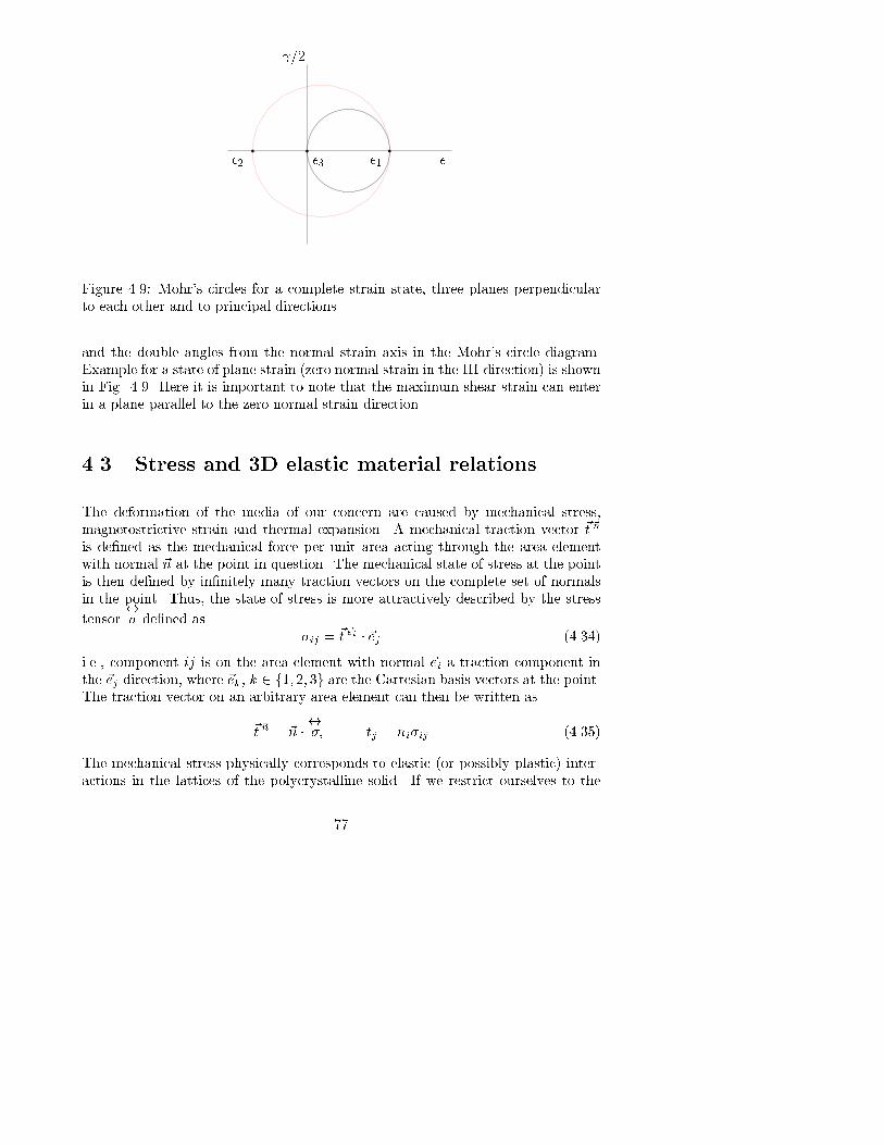
=2
��1�2 �3
Figure 4.9: Mohr's circles for a complete strain state, three planes perpendicular
to each other and to principal directions.
and the double angles from the normal strain axis in the Mohr's circle diagram.
Example for a state of plane strain (zero normal strain in the III-direction) is shown
in Fig. 4.9. Here it is important to note that the maximum shear strain can enter
in a plane parallel to the zero normal strain direction.
4.3 Stress and 3D elastic material relations
The deformation of the media of our concern are caused by mechanical stress,
magnetostrictive strain and thermal expansion. A mechanical traction vector ~t ~n
is de�ned as the mechanical force per unit area acting through the area element
with normal ~n at the point in question. The mechanical state of stress at the point
is then de�ned by in�nitely many traction vectors on the complete set of normals
in the point. Thus, the state of stress is more attractively described by the stress
tensor$� de�ned as
�ij = ~t ~ei � ~ej (4.34)
i.e., component ij is on the area element with normal ~ei a traction component in
the ~ej direction, where ~ek; k 2 f1; 2; 3g are the Cartesian basis vectors at the point.The traction vector on an arbitrary area element can then be written as
~t ~n = ~n � $�; tj = ni�ij (4.35)
The mechanical stress physically corresponds to elastic (or possibly plastic) inter-
actions in the lattices of the polycrystalline solid. If we restrict ourselves to the
77

�yx
�xy��xy
��yx
Figure 4.10: Moment equilibrium on an area element
elastic case, we de�ne a linear elastically isotropic constitutive relation by
�x =1
Y�x � �
Y�y � �
Y�z
�y =1
Y�y � �
Y�z � �
Y�x
�z =1
Y�z � �
Y�x � �
Y�y
xy =1
G�xy
yz =1
G�yz
zx =1
G�zx
where �i denotes normal stresses, �ij denotes shear stresses (stress components
parallel to the area element the action goes through) and the analog notation is
used for strain. Here some points may need to be clari�ed. First we note that only
six components of the stress tensor is used, and that is due to the fundamental
assumption of local moment equilibrium, which leads to a symmetric stress tensor,
�xy = �yx etc. Fig. 4.10 best illustrates the derivation of this property. The
elasticity modulus Y describes normal strain due to parallel uniaxial normal stress
(i.e. only one normal stress component non-zero). Poisson's constant � describes
the ratio of lateral contraction to longitudinal elongation. The shear modulus Gdescribes a proportionality of the shear stress to the resulting shear angle. In
this speci�c case, the shear modulus can be shown to be expressible in the other
78

constants,
G =Y
2(1 + �)(4.36)
due to the fact that pure shear (no normal stresses) on an element can be expressed
as pure normal stresses on a rotated element, the deformation of which is describable
in terms only of Y and � when isotropy (and linearity ) holds.
An orthotropic material is characterized at a point by three mutually orthogonal
directions in which the elastic moduli are extremal2 ,so called principal material
directions, and the elasticity for directions re ected in the planes normal to the
material directions is symmetric. A shear stress won't a�ect the normal strains in
the coordinate system of shear stress application, just like the isotropic case. The
orthotropic material relation is here given by8>>>>>><>>>>>>:
�x�y�z�xy�yz�zx
9>>>>>>=>>>>>>;
=
26666664
E11 E12 E13 0 0 0
E12 E22 E23 0 0 0
E13 E23 E33 0 0 0
0 0 0 G12 0 0
0 0 0 0 G23 0
0 0 0 0 0 G31
37777775=
8>>>>>><>>>>>>:
�x�y�z xy yz zx
9>>>>>>=>>>>>>;
(4.37)
where ~ei; i 2 fx; y; zg are the material principal directions at the point. We see
that nine independent coe�cients are used in this case. The most general linear
anisotropic material would need twenty-one coe�cients in the matrix relating local
stress to strain, since symmetry of the matrix is sound. A symmetric elasticity
matrix is an expression of reciprocity of the material, meaning that an excitation (a
given normal strain in a given direction, say) will in uence the measured conjugate
quantity (the normal stress in a speci�c direction) in the same manner as if the
directions of excitation and measurement would be interchanged.
The elasticity matrix is readily inverted to give the compliance matrix. Elasticity
coe�cients describe the sti�ness of the material, which might be slightly unsuit-
able in certain applications, where the inverse property is more adequate. Looking
back to the description of the linear isotropic material, we see that it is stated as
a compliance relation, with stress components as input - often regarded as more
intuitively attractive. One also has to note that the elasticity modulus introduced
in the compliance relation as the reciprocal of a compliance coe�cient is not di-
rectly identi�able with an elasticity coe�cient, since lateral contraction ratios (and
more generally non-diagonal compliance matrix elements) will in uence the diago-
nal elasticity matrix elements.
2The directions are mutually orhogonal when the orthotropic elasticity matrix is symmetric.
79

4.4 2D elastic material modelling
Elastic behaviour for a GO material can be written with a matrix,
24 �Ex
�Ey Exy
35 =
264
1Yx
� �xyYy
0
� �yxYx
1Yy
0
0 0 1Gxy
37524 �x
�y�xy
35 (4.38)
where �E is the elastic part of the strain (as there might be a magnetoelastic part
also). The diagonal elements Y �1x and Y �1
y are the reciprocals of elastic moduli
measured at states of uniaxial stress. The matrix above contains the compliance co-
e�cients for an orthotropic material. For GO electrical steel, Yy = 200GPa; Ex =
150 GPa; �xy = 0:4; �yx = 0:3; Gxy = 75 GPa is a starting point for numerical
experimentation. Data given by Surahammar AB in their product catalogs show
the elastic modulus as a function of angle to rolling direction. When applying an
uniaxial stress in a direction other than the x or y direction, the compliance matrix
can be transformed to the coordinate system with the uniaxial direction as x' direc-
tion to get the strain parallel to the stress axis (called normal direction), the strain
orthogonal to that axis and the shear in the x'y' system. Such a transformation has
been carried out in section 5.13 for the magnetoelastic case, but it holds also for the
purely mechanical case. By plotting the so produced compliances over angles, the
model can be compared to catalog data. Such a transformation has been carried
out for the values given above. The polar plots based on those values are seen in
Figs. (4.11), (4.12) and (4.13).
Due to the texture, the principal strain coordinate system won't be codirected with
the principal stress system, see Fig. 4.14. There will be an angle between the stress
axis and the largest strain axis. The angle is nonzero for stress neither aligned
with the preferential direction of the texture nor at right angles to the preferential
direction of the texture.
4.4.1 Magnetostriction components and constitutive relations
Magnetostriction lambda is a fractional elongation of a solid ferromagnetic piece
due to homogeneous magnetization with ux density B. For non-saturating uxes,a parabolic expression
� =1
�0PB2 (4.39)
seems to be adequate to describe the main quantitative feature of the phenomenon.
Noting that B2 might be perceived as a magnetic stress, the following simple
80

Normal elastocompliance [1/Pa]
1e-12
2e-12
3e-12
4e-12
5e-12
6e-12
7e-12
30
210
60
240
90
270
120
300
150
330
180 0
+
Figure 4.11: Normal elastic compliance as function of angle of uniaxial stress to
rolling direction.
81

Orthogonal elastocompliance [1/Pa]
4e-13
8e-13
1.2e-12
1.6e-12
2e-12
30
210
60
240
90
270
120
300
150
330
180 0
-
Figure 4.12: Orthogonal elastic compliance as function of angle of uniaxial stress
to rolling direction.
82

Shear elastocompliance [1/Pa]
4e-13
8e-13
1.2e-12
30
210
60
240
90
270
120
300
150
330
180 0
-
+-
+
-
+ -
+
Figure 4.13: Shear elastic compliance coe�cients as functions of angle of uniaxial
stress to rolling direction.
σ
ε2
ε1
Figure 4.14: Uniaxial stress � applied obliquely to a texture. Shows rotation of the
principal strain system �1; �2 compared to the principal stress system.
83

isotropic magnetoelastic constitutive relation is proposed
�Mx =1
�0BxBx � �
�0PByBy � �
�0BzBz (4.40)
cycl:; cycl: (4.41)
Mxy =1
Q
1
�0BxBy (4.42)
cycl:; cycl: (4.43)
By analogy with pure elasticity, P is called the magnetoelastic modulus, Q is called
the magnetoelastic shear modulus, and � is the magnetoelastic transversal contrac-tion ratio. This constitutive relation is isotropic and linear in a magnetic stress
tensor BiBj ; i; j 2 f1; 2; 3g.
P can be quite widely varying for di�erent ferromagnetic metals and alloys, but � isprobably often very close to 0:5, since volume magnetostriction (i.e magnetostrictionaccompanied by volume change) is seldom seen even for high �eld strengths. Volume
magnetostriction is characterized by a nonzero cubical dilatation D0. No volume
magnetostriction is then characterized by DM0 = 0, which means
D0 = �Mx + �My + �Mz = 0 (4.44)
1�0P
B2x +
1�0P
B2y +
1�0P
B2z � �
�0P(B2
y +B2z +B2
z +B2x +B2
x +B2y) = 0 8Bi
) � = 0:5
In solid mechanics, materials with a Poisson ratio of 0:5 are called incompressible,
where compression is in the hydrostatic (volume) sense.
The magnetic stress 1�0B2 is for 1 T ux density (4� � 10�7)�1 � 0:75N=mm2.
One can compare to steel with E = 200GPa at an elongation of 1 �m/m, giving� = 0:2 N=mm2. So even though same magnetic stress and elastic stress will
produce di�erent strain responses due to the di�erent nature of the mechanisms in
the material, the stresses for strains and uxes in the range expected will not be
far apart in order of magnitude.
As previously said, it has to be noted that the constitutive relation 4.40 is suited
only for unoriented, isotropic materials, such as those silicon-iron alloyed cores
used as ux conductors in electrical machines. Oriented silicon-iron is used in large
generators and transformers, therefore an extension to orthotropic conditions is
useful. If ones uses the symmetric magnetic stress tensor BiBj , one can write an
84

magnetostrictively orthotropic relation as
1
�0
8>>>>>><>>>>>>:
B2x
B2y
B2z
BxBy
ByBz
BzBx
9>>>>>>=>>>>>>;
=
26666664
P11 P12 P13 0 0 0
P12 P22 P23 0 0 0
P13 P23 P33 0 0 0
0 0 0 Q1 0 0
0 0 0 0 Q2 0
0 0 0 0 0 Q3
37777775
8>>>>>><>>>>>>:
�Mx�My�Mz Mxy Myz Mzx
9>>>>>>=>>>>>>;
(4.45)
4.4.2 Elasticity and compliance matrices
The above section stated magnetoelastic relations with a compliance formulation
for 2D and an elasticity (sti�ness) relation for 3D. It is of importance to have both
compliance and sti�ness matrices ready for use in various cases of analysis, like
with the �nite element method, treating cubical dilatation and strain descriptions
in di�erent coordinate systems. The inverse of the elasticity matric is called the
compliance matrix.
When the shear components are simply related as in the preceeding section, a
relation which holds for the coordinate axes directed parallel with the structure axes
in the material, it is su�cient to look at the matrix P relating normal components,
P =
24 P11 P12 P13
P12 P22 P23P13 P23 P33
35 (4.46)
The inverse can be found by writing the cofactor matrix and dividing by the deter-
minant,
cof(P ) =
24 P22P33 � P23P23;�(P12P33 � P23P13; P12P23 � P22P13�(P12P33 � P13P23); P11P33 � P13P13;�(P11P23 � P12P13)P12P23 � P13P22;�(P11P23 � P13P12); P11P22 � P12P12
35
det(P ) = P11(P22P33 � P23P23)� P12(P12P33 � P23P13) + P13(P12P23 � P22P13)
P�1 =1
det(P )cof(P )
It is seen that both P and its inverse are symmetric. The cubical dilatation can
now be written
D0 =1
�0det(P )fB2
x(P22P33 � P23P23 � P12P33 + P13P23 + P12P23 � P13P22) +
B2y(�P12P33 + P23P13 + P11P33 � P13P13 � P11P23 + P13P12) +
B2z (P12P23 � P22P13 � P11P23 + P12P13 + P11P22 � P12P12)g
85

A note about the case when there is isotropy is in place. After setting P11 =
P22 = P33 = a; P13 = P23 = P12 = b, the transverse sti�ness coe�cient will be
�b=(a � b)(a + 2b). One can see that a positive b smaller than a gives a negative
(contractive) transverse compliance coe�cient. The positive transverse sti�ness
coe�cient describes a sti�ening e�ect between orthogonal directions, at a given
state of strain there will be a transverse contraction tendency requiring a larger
orthogonal stress to provide the strain. The determinant of P is (a � b)2(a + 2b),and zero for b = �0:5a and a = b, for which the sti�ness matrix is not invertible
into a compliance matrix. If the sti�ness matrix is not invertible, stress cannot
appear in any state, there are restrictions on allowable states. As restrictions are
more likely to exist on the allowable strain states, like no dilatation or no shear, it
is more likely the compliance matrix that is singular. With negative o�-diagonal
entries (necessary in elasticity, not strictly necessary in magnetoelasticity), zero
dilatation will happen at o�-diagonal entry value half of diagonal entry value.
Even though it is the compliance matrix that is more important for analysis, and a
bit simpler to understand, the sti�ness matrix is needed to form the local sti�ness
matrix of the FE method. Whatever is given, we need to form the inverse (if
possible). A simple approximation can be derived for the 3D case.
P�1 �
264
1P11
� P12P11P22
� P13P11P33
� P12P11P22
1P22
� P23P22P33
� P13P11P33
� P23P22P33
1P33
375 (4.47)
From this approximation, one can see that there are six orthogonal contraction
ratios in the orthotropic case, P12=P22, P13=P33, P23=P33, P12=P11, P13=P11 and
P23=P22. One can also deduct the approximate relations between the compliance
coe�cients when there is never any dilatation: P12=P22 + P31=P33 = 1, cycl., cycl.
Exact inverses are simplest to obtain for 2D cases. Isotropic compliance matrix to
elasticity matrix inversion can be written as�1Y � �
Y
� �Y
1Y
��1=
1
1� �2
�Y �Y�Y Y
�(4.48)
with the trivial shear part left out. Orthotropic elasticity matrix to compliance
matrix inversion is written as�E11 E12
E12 E22
��1=
1
E11E22 �E212
�E22 �E12
�E12 E11
�(4.49)
Because the inverse of the symmetric matrix is also symmetric, the relation can be
used also for compliance to sti�ness inversion.
86

The entries of the inverse of the 3D general matrix P above can be calculated to
P�111 =
1
P11(1� P 2
23
P22P33)=N (4.50)
P�112 = � P12
P11P22(1� P23P31
P12P33)=N (4.51)
P�123 = � P23
P22P33(1� P31P12
P23P11)=N (4.52)
P�131 = � P31
P33P11(1� P12P23
P31P22)=N (4.53)
N = 1� P 212
P11P22� P 2
23
P22P33� P 2
31
P33P11+ 2
P12P23P31
P11P22P33(4.54)
where N is a help constant for the denominator of the components of the inverse.
In deriving the inverse, it is helpful to note that only two cofactor elements need to
be calculated, namely cof(A)11 and cof(A)12, wherefrom the other elements can
be gotten from cyclic permutation of indices.
Reciprocity can be investigated more simply with the approximate inverse. If a
traction t is applied in the z-direction, say, there will be a strain 1P33
t in the same
direction, an equivalent stress P31P33
t in the x-direction and a strain 1P11
P31P33
t in the x-direction. One cannot call the in uence on the orthogonal direction stress because
it is natural and stress free. After swapping source (traction) and measurement
(strain) directions we get an uniaxial stress in the x-direction that will give a strain1P33
P13P11
t in the z-direction. So the fact that P13 = P31 manifests itself in reciprocity.Transverse contraction ratios describe strain at right angles to a given strain, so
they are less fundamental than the reciprocal moduli.
4.5 Equations of equilibrium and motion
4.5.1 Force equilibrium
The 2D force equilibrium equations are
@x�x + @y�yx + fbx = 0 (4.55)
@x�xy + @y�y + fby = 0 (4.56)
The �rst equation of these expresses force equilibrium in the x direction, while the
second is for the y direction. �i; i = x; y are normal stresses on the side of a cut
which has a lower coordinate from the side with higher coordinate. The cut has a
87
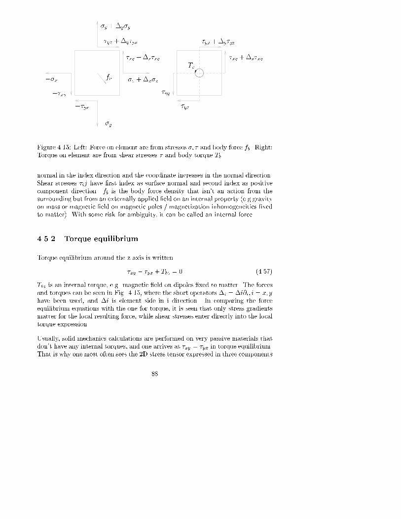
�y +�y�y
�yx +�y�yx
�xy + �x�xy
�x +�x�x
��yx
��xy
Tv
�xy +�x�xy
�yx +�y�yx
fv
��y
��yx
��xy
��x
Figure 4.15: Left: Force on element are from stresses �; � and body force fb. Right:Torque on element are from shear stresses � and body torque Tb.
normal in the index direction and the coordinate increases in the normal direction.
Shear stresses �ij have �rst index as surface normal and second index as positive
component direction. fb is the body force density that isn't an action from the
surrounding but from an externally applied �eld on an internal property (e.g gravity
on mass or magnetic �eld on magnetic poles / magnetization inhomogeneities �xed
to matter). With some risk for ambiguity, it can be called an internal force.
4.5.2 Torque equilibrium
Torque equilibrium around the z-axis is written
�xy � �yx + Tbz = 0 (4.57)
Tbz is an internal torque, e.g. magnetic �eld on dipoles �xed to matter. The forces
and torques can be seen in Fig. 4.15, where the short operators �i = �i@i; i = x; yhave been used, and �i is element side in i direction. In comparing the force
equilibrium equations with the one for torque, it is seen that only stress gradients
matter for the local resulting force, while shear stresses enter directly into the local
torque expression.
Usually, solid mechanics calculations are performed on very passive materials that
don't have any internal torques, and one arrives at �xy = �yx in torque equilibrium.That is why one most often sees the 2D stress tensor expressed in three components
88

instead of four (six instead of nine in 3D). The addition of an internal torque
will create a di�erence between shear stresses, a di�erence which will balance the
internal torque in equilibrium. Since the unsymmetrical shear stresses also will
appear in the force equilibrium equation (where the torque doesn't enter), the
di�erence will give rise to an additional rotation of the element. In the constitutive
relation, the shear stress asymmetry will give a shear strain that is a�ected only by
the symmetrized shear stress, so the strain tensor is still symmetric. A tentative
symmetrization of the shear stress can be written as a simple average � 0xy = (�xy +�yx)=2, and then the normal shear modulus can be used to relate to the strain.
4.5.3 Equations of motion, coordinate types
If the acceleration of elements is non-negligible, the equilibrium equation has to be
modi�ed into the equation of motion,
@x�x + @y�yx + fx = �@2t u (4.58)
cycl: (4.59)
cycl: (4.60)
(4.61)
Another way of writing it is as r � $� + ~f = �@2t ~u. The coordinates used to write
the �eld is really initial/material coordinates here. It matches with the de�nitions
of strain used. If the space coordinates were used, the acceleration of the single
particle or element at (x; t) would be the sum of the �eld speed change at a space
point (with di�erent particles passing) and the �eld gradient times the distance
the actual particle travels per time unit. That case would give a second term to
the right hand side, which would not dominate for small strains (�rst term linear
in strain and second quadratic from a plane wave ansatz). In fact the �rst term
becomes equal to the right hand side in the material coordinate case. Thus there is
no need to make a distinction between the coordinate types from a strain viewpont,
but when visualizing magni�ed computed solutions in terms of displacements, it is
clearest to use grid coordinates as o�sets for displacement (i.e grid coordinates are
material coordinates) and not as results of displacement.
4.5.4 Translatory and rotatory equations of motion
Basic postulates governing the motion of the continuum are
~F = _~p (4.62)
~T =_~L (4.63)
89

where F is the force acting on the continuum enclosed by a volume V , T is the
torque on that volume, p is the momentum and L is the angular momentum. The
equations should hold for any part V of the continuum. From this statement the
equation of translatory motion and the equation of rotation can be derived.
The equations of motion are simple to derive in di�erential form by componentwise
equating the force on an element with inertia. Force comes from stress and so
called body forces, typically gravity (see section below). In the x-direction for a
2D-element one gets
@x�x + @y�yx + fbx = ��u (4.64)
Cyclic permutation of di�erentiation variable and component index give the equa-
tion for the y-direction. A 3D object can be treated with the two equations if there
is no traction on the z-normal surface, a case called plane stress. When counting
dimensions as the number of independent variables, it is a 2D problem.
The equations of equilibrium are achieved when the continuum is at rest, simply
leaving the right hand side in the equations of motion identical to zero.
4.5.5 Body forces
The body force is typically a volume force from gravity, ~fb = �g ~eg.
Magnetic body forces, i.e. magnetic force density distributed over the volume,
can be present when the magnetic material is inhomogeneous. Stratton gives the
formula
fv = �1
2H2r� (4.65)
for this body force, saying that the forces are directed from high permeability spots
to spots of low permeability. As the materials de�nitely are nonlinear, there will
be di�erences in permeability when the specimen is inhomogeneously magnetized.
Another formula given by Stratton states the surface force density fs,
~fs = �( ~H � ~n)� 1
2�H2~n (4.66)
which can be simpli�ed to
~fs =1
2�H2~n (4.67)
when the magnetic �eld strength ~H is normal to the surface, that could be a good
approximation for real high permeability materials.
90

Cheng [97] presents a derivation of attraction of two perfect permeable materials
where he �nds the e�ective surface force density from the magnetic energy derivative
with respect to position change of the yoke. The result is
~fs =1
2BH~n (4.68)
where the value of H is taken on the air side of the air-yoke interface.
Binns and Lawrenson [98] make an equivalent con�guration with magnetic surface
poles at the air-yoke interface with replacement of the magnetic material with air.
The force equation is~fs = �m ~H (4.69)
where �m is the magnetic surface pole density.
Becker [99] states the body force by using the magnetization ~M directly,
fv = ( ~M � r) ~B (4.70)
In applying this equation, the user will still get problems due to kinks in the ap-
proximated ux lines.
4.6 Magnetic stress
Based on the constitutive relations 4.40 and 4.42 , a tensor was identi�ed that can
be regarded as the driving magnetic stress,
�Mx =1
�0B2x
�My =1
�0B2y
�Mxy =1
�0BxBy
�Myx =1
�0ByBx
Maxwell stated an asymmetric stress by using the externally applied �eld strength
H in addition to B,
�Mx = BxHx � 1
2�0H
2
�My = ByHy � 1
2�0H
2
91

�Mxy = BxHy (4.71)
�Myx = ByHx
He called the tensor P and used another unit system [100] but the above is the
same within a scalar factor. He derived it by �rst restating the expression fvmx =~B � rHx � 1
2ddx�0(H
2) into fbmx = ddx[BxHx � 1
2�0H
2] under the condition that
the H-�eld should be divergenceless. The formula for the torque stated as Tbmz =
BxHy �ByHx. By using the force and torque density to stress equations,
fbmx =d
dx�Mx +
d
dy�Myx (4.72)
Tbmz = �Mxy � �Myx (4.73)
he could identify the expressions 4.71. His equations for stress are the general ones
and covers the case with non-aligned magnetization to magnetic �eld intensity.
Field intensity doesn't have to be strictly externally applied, it can also come from
magnetization discontinuities or inhomogeneities as discussed earlier.
92

Chapter 5
Models of magnetostriction
5.1 The interplay between mathematical modeling
and physical experimenting
Measurements are needed both to validate made models and to inspire the making
of models. This interplay can occur on di�erent levels of physical scale and on
di�erent types of problems. Three kinds of problems are separable to the engineer:
material, component and system problems. Measurements can be done on all types
and levels of problems, but in the present instance, measurements are only done on
a macroscopic material problem. The measurement provides parametric input to
a model of the material properties. The model is made to �t into a �nite element
program, that is in turn able to model a component such as a core. The core model
might be studied to provide a simpli�ed, single element, model to be included in
a greater system model. Ideally, the component and the system should be veri�ed
with measurements of the corresponding type. All these steps are time-consuming
but not impossible to be carried out by people.
The most di�cult task is to bridge the gap between the microscopic and the macro-
scopic levels. A microscopic model often consists of an ideal part and part originat-
ing from a small number of defects or only one defect. The real situation di�ers in
that the defects are neither of a small number nor approaching an in�nite number.
In the in�nite limit the model might be possible to average, but real components
well represented by it could be bad. In the intermediate range automated math-
ematical tools together with elaborate physical equipment are needed to map the
defects and their e�ects. Parameter selection from a standpoint on the grounds of
93

thermodynamics and causality could lead to simpli�ed macroscopic models.
Other divisions of models into classes can also be done. One such division is with
continuum, parameterized and physical models. Again, a complete description also
suitable for use in engineering analysis would need to bridge the model types. There
is seldom the case that this can be achieved. In his speci�c instance, the author
wanted to make measurements and use a parameterization that was sound and
could �t the �nite element method of solving engineering problems.
5.2 Continuum model
The activity to include continuum magnetostriction phenomena in computational
tools for magnetomechanics [92] has spawned an interest in the exploration of possi-
ble mathematical ways to represent the material response in a su�ciently accurate
manner. Here, we take into account the dynamic behaviour of magnetostriction as
described by what is commonly known as butter y loops. When a harmonic ux
density is present, the measured magnetostriction loop is a curve with two branches
when plotted against the ux density. Although often thought of as related to hys-
teresis, we believe that the lag of magnetostrictive strain can be e�ectively modelled
by a rate-dependency model, which properly assigns the phase shifts to the mag-
netostriction harmonics. We deal at length with the case of linear orthotropic
elasticity and linear anisotropic magnetoelastic behaviour. By linear magnetoelas-
ticity it is meant that the magnetostrictive strain$�M is linear in the magnetic stress
tensor BiBj . By knowing that there is a weak coupling on permeability from stress,
we are able to separate the simulation into one magnetic part and one mechanical
part, where the magnetostrictive strains appear as sources to the total strain. The
main interest in the results lies in an evaluation of the in uence of elastic properties
on measurable total strain in a sheet excited by the yoke pair described elsewhere
in this text.
By using the rate-dependent, dispersive, model in stead of a true hysteresis model
we get mathematical simplicity and easier veri�ed thermodynamic compatibility.
Simplicity gives speed of computation and a more de�nitive ability to consider
rotational hysteretic phenomena. As mentioned before, we foresee that there will
also be considerable rate-dependency in magnetostriction, for which we will use a
nonlinear dispersion law.
94

-1.5 -1 -0.5 0 0.5 1 1.5-3
-2
-1
0
1
2
3
4
5
6
Flux density [T]
Mag
neto
stric
tive
stra
in [m
icro
m/m
]
Figure 5.1: Butter y loops of negative valued �Mx vs. Bx and positive valued �Myvs. By.
95

5.3 Butter y loops
Are the �M [B] loops hysteretic in its true sense or are they a re ection of a time-
rate-dependent, dispersive, phenomenon? The simplest proposition of a dispersive
governing di�erential equation is
_�M [B] = k(�Mntr(B)� �M [B]) (5.1)
where �Mntr is the strain at an ideal process with no time rate of change of strain.
This ideal strain can be investigated by exciting the material with a ux of very
low frequency. The bracketing of the arguments to the strains in the formula shows
the dependence of history of the argument. (�) means that there is no dependenceon past history and [�] means that there is a dependence of the time history of the
argument.
The time domain equation can be Fourier transformed into a frequency domain
equation for a speci�c ux density process (time behaviour),
j!~�M (!) = k(~�Mntr(!)� ~�M (!)) (5.2)
from which an equation between the no-time-rate-strain and the actual strain is
obtained,
~�M (!) =k
j! + k~�Mntr(!) (5.3)
The frequencies present in the spectrum of the magnetostrictive strain is di�erent
from those present in the ux density, since the no time rate dependent strain is
even in ux density. If B is harmonic at the frequency f , the fundamental frequencyof �M will be 2f . As the magnetostriction curve shows a saturation e�ect, there
will be higher powers in the nonlinear �Mntr(B) function. Those even powers will
produce even harmonics in �M compared to the B harmonic.
If B is anharmonic with a fundamental of f , the spectrum of �M becomes more
complicated. There will be harmonic interaction through the nonlinearity, and the
crossproducts will give addition and subtraction of frequencies in B to formmirrored
frequencies in �. These mirrored frequencies will �ll out gaps in the spectrum of
the strain compared to when having a purely harmonic ux density.
The equation 5.1 was a dispersive relation for a simple case of rate-dependency. A
general dispersive relation can be written
u(t) = K(t) ? i(t) (5.4)
~u(!) = ~K(!) �~i(!) (5.5)
where i is the input variable, u is the output variable, ? is the convolution operatorand K is the kernel describing the properties of the medium without reference to
96

a speci�c time trace of the input variable. In the rate-dependency case above,~K = k=(j! + k) and i(t) = �Mntr(B(t)). As the time rate independent strain is
nonlinear in the ux density, it is tempting to call the � � B relation a nonlinear
dispersive one. It is not a good term though, as a di�erential equation governing
the nonlinear dispersive process would contain a time-derivative term with a higher
power than one, rather than the driving term containing higher powers as the rate-
dependency case above.
5.4 Rate-dependency model
We introduce a scalar magnetostriction rate-dependency model in the time and
frequency domains as
_� = k(B2
�0P� �) (5.6)
~� =k=�0P
jn!1 + kFfB2g (5.7)
where k is a lag parameter and P is a magnetoelastic modulus. The following
relations apply when there are only discrete harmonics,
g(t) = F�1f~gg =1Xn=0
Ref~g(n)ejn!1tg (5.8)
~g(n) = Ffgg (5.9)
where n is the number of the harmonic to the fundamental frequency !1. The sumin Eq. (5.8) is the Fourier series of the time signal g(t), and Eq. (5.9) symbolizes
the Fourier decomposition of g(t) into the Fourier coe�cients ~g(n) that are the
discrete spectrum of g(t). Restricting what follows to the case of a harmonic ux
density of angular frequency !1, one has
FfBiBjg = dBiBj1
2�n0 + dBiBj
1
2�n2 (5.10)
where BiBj ; i; j 2 fx; yg is a magnetic stress tensor and �nm is the Kronecker
delta. When the ux density is uniaxially alternating, the peak values of the tensor
components can be written dBiBj = BiBj . As butter y loops are given for the
harmonic case, we are able to identify the k-parameter in a simple manner. One
can show that an approximation of the vertical width b of the loop is
b =1
�0P
4!1k
qB2 �B2
mBm (5.11)
97

from which k can be determined, as Bm is the ux density where the width is
measured. This holds when the damping introduced by the model is negligible, i.e
when 2!1 � k. Phase shift can in that case still be considerable, allowing loops
with fair width to be represented.
5.5 Simple 2D magnetostriction models
A simple isotropic constitutive relation for nonoriented silicon iron in thin (0.5 mm)
sheets (motor steel) can be written as8<:
�Mx�My Mxy
9=; =
24 1
P� �P
0
� �P
1P
0
0 02(1+�)P
35 1
�0
8<:
B2x
B2y
BxBy
9=; (5.12)
A parameterization like this is at least mathematically sound as B2x,B
2y and BxBy
are the components of a tensor in the x-y system, i.e. it obeys strain like component
transformation to rotated coordinate systems. Statements taken by analogy from
elasticity say that � = 0:5 holds due to magnetoelastic isotropy and that the shear
modulus can be written as P=2(1 + �) due to isotropy and linearity.
Oriented silicon iron in 0.3 or 0.23 mm thin sheets (transformer steel) is tried to be
included in the simple scheme by the relation
8<:
�Mx�My Mxy
9=; =
264
1Px
D12 0
D211Py
0
0 0 1Gxy
375 1
�0
8<:
B2x
B2y
BxBy
9=; (5.13)
where the Dij :s and reciprocals of moduli can be called magnetocompliance coe�-
cients.
5.6 Magnetoviscoelastic models
Magnetostriction models can be classi�ed into two main groups: magnetoelasto-
plastic and magnetoviscoelastic. Plastic models are time-rate independent of the
excitation, while viscous models are rate-dependent. The model development for
the magnetoviscoelastic case is reported in the following subsections.
98

5.6.1 Quasistatic linear case
This case can be written on the form �M = 1P�0
B2. It is linear in the magnetic
stress 1�0B2. The proportionality constant P has been called the magnetoelastic
modulus [101]. No time derivative is present in this constitutive relation, so it can
be useful when time-rate of the magnetic stress is low, which is the quasistatic case.
For a two-dimensional continuum one might apply an isotropic version as
�Mx =1
�0P
�B2x � �B2
y
�(5.14)
�My =1
�0P
�B2y � �B2
x
�(5.15)
Mxy =2(1 + �)
�0PBxBy (5.16)
where the expression for the shear magnetostriction Mxy is obtained from the as-
sumption of both linearity and isotropy. The constructed magnetic stress tensor1�0BiBj ; i; j 2 fx; yg obeys proper tensorial transformation laws. � is a magnetoe-
lastic Poisson ratio. One has to note that in continuum problems, the total strain$� satisfying the equilibrium and boundary equations will consist of an elastic part$�E and the magnetoelastic part
$�M . The complete constitutive relation for linear
isotropy is then
�x =1
Y(�x � ��y) +
1
�0P
�B2x � �B2
y
�(5.17)
�y =1
Y(�y � ��x) +
1
�0P
�B2y � �B2
x
�(5.18)
xy =2(1 + �)
Y�xy +
2(1 + �)
�0PBxBy (5.19)
where the stress$� is related through the elastic modulus Y and Poisson ratio � to
elastic strain$�E only.
5.6.2 Rate-dependent linear case
One simple type of rate-dependency can be written in the time-domain as _�M =
k( B2
�0P� �M). It is of �rst order in time derivatives and uses a single parameter k to
represent response speed. The reciprocal of k is a lag time constant. The simple lagbehaviour might be found for excitations that do not signi�cantly enter frequency
regions with material resonances. By plotting �M versus B one gets the butter y
99

curve. The curve for such a simple case is with only one crossing at B = 0, an
example of which is shown in Fig. 5.1 at 50 Hz and for two directions of ux and
strain.
Continuing in the frequency domain, the �rst order relation is written as ~�M =1
�0Pk
j!+kfB2, where ! is angular frequency. In a 2D case, it is convenient to ab-
sorb the frequency dependent factor into magnetocompliance coe�cients Dij =1Pij
kjn!1+k
. For an anisotropic material one can then write
e�Mx =D11
�0fB2x +
D12
�0fB2y
e�My =D21
�0fB2x +
D22
�0fB2y (5.20)
e Mxy =D33
�0gBxBy
in a coordinate system positioned relative to the material texture such that shear
strain is independent of x� and y� magnetic stress components. In fact mag-
netostrictive shear strain seems to be negligible when x� and y� directions are
chosen to be coincident with rolling and transverse directions of highly anisotropic
silicon-iron [102]. In those cases D33 can be set to zero. This does not mean that
shear magnetostriction is zero in all coordinate systems. The linear case is easy to
implement in computation programs.
5.6.3 Rate-dependent nonlinear case
Of interest is the plot �M to B2, which can be seen as a strain-stress diagram,
yielding magnetoelastic potential energy from an averaged single-valued curve and
a loss proportional to the area of the loop. This case uses an arti�cial non-lossy,
i.e single-valued, butter y curve �MA(B2). The single-valued constitutive relation
is found from least squares polynomial �tting to the vertical mean curve of the two
branches. One can use scaled Legendre polynomials translated to the argument
interval [0; 1] to form an orthogonal function sequence ffig. This sequence makes iteasy to alter and evaluate the polynomial order of the approximation. For a third
order model, able to cover moderately wavy butter y loops, one can write
�MA(B2)=�MA = d0 + d1f1(B2=B2
s ) + d2f2(B2=B2
s ) + d3f3(B2=B2
s ) (5.21)
where Bs is the ux density at the striction peaks. Lossy (double-valued) mag-
netostriction �M is dependent on frequency and non-lossy magnetostriction, ~�M =
H(f)~�MA. A three parameter resonant transfer function H(f) can be formulated as
H(f) =�(f=fd2)2 + 1
�(f=fr2)2 + jf=fr1 + 1(5.22)
100
This function was used in [94] for transversal strain and ux density. Resonance
can be seen as additional crossings at non-zero ux densities in the butter y curve
or larger than 90� phase shifts between non-lossy and lossy magnetostriction at theresonance frequency fr2. The zero response at fd2 is needed to restore amplitude
and phase for higher measured harmonics. Additional measurements can be carried
out to investigate if this zero is physical or if an additional parameter is needed
to move the zero out into the complex plane. To simulate the magnetostriction
response for cyclic processes it is convenient to use frequency domain techniques
which allows the application of H(f) directly instead of solving the corresponding
ordinary di�erential equation with numerical time-stepping.
The di�culty arising is the amount of algebra that has to be done to sort out the
harmonic interaction of Fourier components that occurs due to nonlinearity. As
an example for a case without excessive waveform distortion, three odd harmonics
of the ux density signal might be enough to represent it. The quadratic relation
between ux density and magnetic stress then gives �ve even harmonics in the
magnetic stress for the example and then the third order nonlinearity in Eq. (5.21)
gives 15 even harmonics in the magnetostriction. The algebra will be presented in
detail in chapter 8.
5.7 Model incorporation in plane stress calcula-
tions
We assume that plane stress prevails in the sheet whose strain �eld is to be com-
puted. It is also assumed that inertia e�ects can be neglected, which is the case if
we consider the sheet being mass-less or if the time derivative of excitation is low.
Performing the decomposition as shown in Eqs. (5.8), equilibrium equations and
strain-displacement equations are written in the frequency domain as
@x~�x + @y~�xy = 0 ~�x = @x~u
@x~�xy + @y~�y = 0 ~�y = @y~v (5.23)
~ xy = @x~v + @y~u
We have to use a constitutive relation suitable for representing both elastic and
magnetostrictive strain. When assuming elastic orthotropy and magnetoelastic
anisotropy in a somewhat restricted sense one can write
~�x = C11~�x + C12~�y +D11
�0FfB2
xg+D12
�0FfB2
yg
~�y = C12~�x + C22~�y +D21
�0FfB2
xg+D22
�0FfB2
yg (5.24)
101

~ xy = C33~�xy +D33
�0FfBxByg
The elastic compliance coe�cients Cij are C11 = 1=Yx, C12 = ��xy=Yy = ��yx=Yx,C22 = 1=Yy, C33 = 1=Gxy. Yx and Yy are the elastic moduli for uniaxial stress in thex and y directions respectively. �xy and �yx are the orthogonal contraction ratios
of the strain in the �rst index direction to the strain in the second index direction
under uniaxial stress in the second index direction. Gxy is the shear modulus
in the xy-coordinate system, which is directed with basis vectors parallel to the
material principal axes. The x-direction is the rolling direction of the sheet and the
y-direction is the transversal direction. Reciprocity holds because of elastic energy
conservation and orthotropy then holds as material principal axes are at right angles
to each other. In the simulations we have used typical values of Yy = 200 GPa,Yx = 150 GPa, Gxy = 74 GPa, �xy = 0:4 and �yx = 0:3.
The magnetoelastic compliance coe�cients Dij we have used are based on and
D011 = �0:0013 GPa�1, D0
22 = 0:02 GPa�1, D012 = �0:037 GPa�1, D0
21 =
0:0013 GPa�1 and D033 = 0. These are taken from data presented for a highly
grain-oriented material in [102]. By coordinate transformation it is seen that nor-
mal magnetoelastic compliance is by far greatest in the y-direction and even greater
is the negative compliance to an orthogonal direction from applied normal magnetic
stress in the y-direction, see Figs. 5.2, 5.3 and 5.4. . The experimental data in
[102] show no shear strain in the x,y-system for a variety of angles of ux density
to rolling direction, so we set the magnetic shear compliance D33 to zero. The
frequency dependent coe�cients Dij are written using the model in Eqs. (5.7),
Dij = D0ij
k
jn!1 + k(5.25)
By using the same k-parameter for all directions, it is seen from the simple formula
Eq. (5.11) that an inherent assumption is that the relative butter y loop width is
constant over all directions when directions are magnetized with the same ampli-
tude, i.e. increasing loop widths with increasing normal magnetocompliance. k wasset to 1600 s�1 and butter y loops for this case are drawn in Fig. 5.1, with ux
density amplitudes of 0.63 T in the transverse direction and 1.2 T in the rolling
direction at frequency 50 Hz. Large relative butter y loop widths are mostly con-
nected with low magnetocompliance, so here are space for improvements in the
description. The restriction on magnetoelastic anisotropy is here that magnetic
shear stress does not in uence normal x,y-strains, something that might be loos-
ened in the future to obtain a better �t with experiments.
102
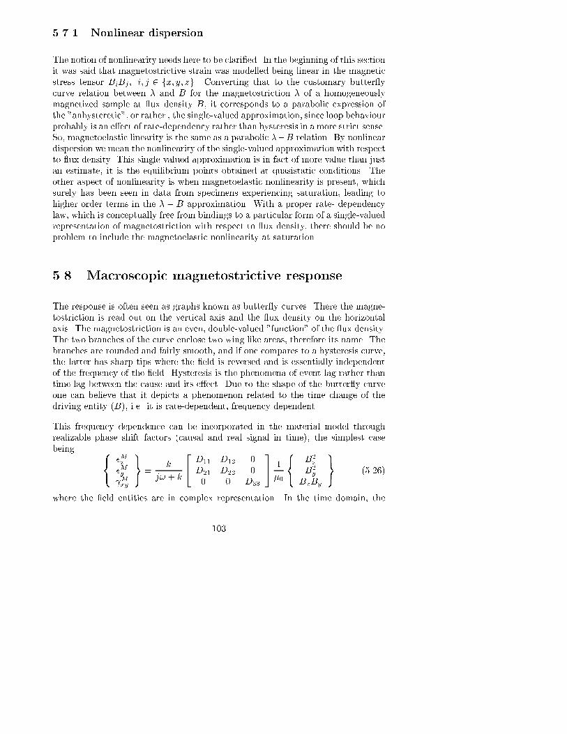
5.7.1 Nonlinear dispersion
The notion of nonlinearity needs here to be clari�ed. In the beginning of this section
it was said that magnetostrictive strain was modelled being linear in the magnetic
stress tensor BiBj ; i; j 2 fx; y; zg. Converting that to the customary butter y
curve relation between � and B for the magnetostriction � of a homogeneously
magnetized sample at ux density B, it corresponds to a parabolic expression of
the "anhysteretic", or rather , the single-valued approximation, since loop behaviour
probably is an e�ect of rate-dependency rather than hysteresis in a more strict sense.
So, magnetoelastic linearity is the same as a parabolic ��B relation. By nonlinear
dispersion we mean the nonlinearity of the single-valued approximation with respect
to ux density. This single-valued approximation is in fact of more value than just
an estimate, it is the equilibrium points obtained at quasistatic conditions. The
other aspect of nonlinearity is when magnetoelastic nonlinearity is present, which
surely has been seen in data from specimens experiencing saturation, leading to
higher order terms in the � � B approximation. With a proper rate- dependency
law, which is conceptually free from bindings to a particular form of a single-valued
representation of magnetostriction with respect to ux density, there should be no
problem to include the magnetoelastic nonlinearity at saturation.
5.8 Macroscopic magnetostrictive response
The response is often seen as graphs known as butter y curves. There the magne-
tostriction is read out on the vertical axis and the ux density on the horizontal
axis. The magnetostriction is an even, double-valued "function" of the ux density.
The two branches of the curve enclose two wing like areas, therefore its name. The
branches are rounded and fairly smooth, and if one compares to a hysteresis curve,
the latter has sharp tips where the �eld is reversed and is essentially independent
of the frequency of the �eld. Hysteresis is the phenomena of event-lag rather than
time-lag between the cause and its e�ect. Due to the shape of the butter y curve
one can believe that it depicts a phenomenon related to the time change of the
driving entity (B), i.e. it is rate-dependent, frequency dependent.
This frequency dependence can be incorporated in the material model through
realizable phase shift factors (causal and real signal in time), the simplest case
being 8<:
�Mx�My Mxy
9=; =
k
j! + k
24 D11 D12 0
D21 D22 0
0 0 D33
35 1
�0
8<:
B2x
B2y
BxBy
9=; (5.26)
where the �eld entities are in complex representation. In the time domain, the
103

model can be symbolically written _� = k(�e � �). �e is a single-valued function
and represents the equilibrium for no change in driving �eld, or when changing the
�eld very slowly, quasistatically. The di�erential equation describes a dispersive
material relation, and because �e is nonlinear in B the resulting ��B dependency
is nonlinearly dispersive.
5.9 Identi�cation of parameters
If the parameters are D11; D22; D12; D21 and k, the following information can be
used to obtain the values of them: k is taken from the butter y wing width or
area. D11 is found from �e � B in the RD direction. It might be negative for
the GO materials. D22 is seen from �e � B in the TD direction. D12 can be
determined from the ratio of RD contraction to TD expansion. D21 is evaluated
by transverse expansion to rolling direction length change. If there is zero volume
magnetostriction, not all of the parameters will be independent. The relations
between them in that case is derived below.
5.9.1 Magnetostrictive incompressibility
The restrictions on magnetoelastic coe�cients when no volume change is assumed
are now derived. 2D forms are uninteresting, area conservation is not an issue, so
only 3D is dealt with. It is simple to look at the expression of the dilatation using
magnetocompliance coe�cients,
�Mx + �My + �Mz =1
�0B2xfD11 +D12 +D31g+
1
�0B2yfD22 +D23 +D12g+ 1
�0B2zfD33 +D31 +D23g = 0 8B2
i (5.27)
For the equation to hold always, the expressions between braces must be zero.
There will be a simple equation system of three equations and six unknowns when
the magnetocompliance matrix is symmetric as above,
D11 +D12 +D31 = 0 (5.28)
D12 +D22 +D23 = 0 (5.29)
D31 +D23 +D33 = 0 (5.30)
yielding three dependent parameters and three independent ones. The solution in
terms of the diagonal compliances is
D31 =1
2(�D11 +D22 �D33) (5.31)
104

cycl: (5.32)
cycl: (5.33)
which is helpful when lateral contraction ratios are wanted from measured data of
compliances in main directions 1.
In situations where only D11, D12 and D22 are given from measurements, like when
only measuring in the plane of the specimen, the other coe�cients are from
D13 = �D11 �D12 (5.36)
D23 = �D12 �D22 (5.37)
D33 = D11 + 2D12 +D22 (5.38)
In some cases one might be given values of sti�ness coe�cients rather than com-
pliance coe�cients. But getting a complete set of sti�ness coe�cients from the
incompressibility condition is impossible. The columns of the compliance matrix in
such a case are linear combinations of each other, which means that the compliance
matrix is singular, non-invertible. It also means that all stress states are permitted,
but not all strain states. Thus the sti�ness matrix in the ordinary sense doesn't
exist. However, we can write a lower dimensional description of sti�ness, and use
one stress component as a parameter to determine the stress state. One splitting
of the compliance relation is��Mx�My
�= D0 1
�0
�B2x
B2y
�+ d03
1
�0B2z (5.39)
�Mz = d0T31
�0
�B2x
B2y
�+D33
1
�0B2z (5.40)
Inversion of the D0 matrix and using the fact that D0�1d03 = [�1;�1]T under the
incompressibility constraints, one gets
1
�0
�B2x
B2y
�= D0�1
��Mx�My
�+
�1
1
�1
�0B2z (5.41)
�Mz = ��Mx � �My (5.42)
1It might be clarifying to write out the de�nitions of lateral contraction and tension ratios.They are here denoted by �ij and ij respectively, and are expressed by
�ijdef
=��Mi
�Mj
j~B=Bj~ej= �
P�1ij
P�1jj
(5.34)
ijdef
=
B2
i
B2
j
j�kl=�kl�kl�lj=Pij
Pjj(5.35)
The lateral tension ratio is de�ned with the denominator being the major applied normal stressand the numerator being the minor normal stress that has to be applied orthogonally to the majorstress to obtain an uniaxial strain state, due to the Poisson transversal contraction e�ect.
105

It is seen that knowledge of two strain components and one stress component gives
knowledge of the stress state. If stress in the z-direction is zero, as it often is in the
sheet samples considered in this book, one can use the 2D sti�ness matrix D0�1,
D0�1 =1
D11D22 �D212
�D22 �D12
�D12 D11
�(5.43)
5.10 Magnetoelastic shear modulus
To get some grip on the magnetoelastic shear modulus, below called Q, one can
study the magnetoelastically isotropic case, which might hold as an approximation
for nonoriented materials. Isotropy means that the magnetocompliances are inde-
pendent of coordinate system. By transforming a sheared state in the xy-system to
the unsheared principal system called the nt-system, one can relate the shear mod-
ulus Q to the normal magnetocompliance D11 and the o�-diagonal (orthogonal)
magnetocompliance D12.
The general strain component transformation from nt to xy can be written
�Mx = �Mn cos2 '+ 2�Mnt cos' sin'+ �Mt sin2 ' (5.44)
�My = �Mt cos2 '� 2�Mnt cos' sin'+ �Mn sin2 ' (5.45)
Mxy = 2(�2 cos' sin'�Mnt + cos' sin'�Mn � cos' sin'�Mt ) (5.46)
The nt-system is a zero shear strain system,
2�Mnt = Mnt = 0 (5.47)
which yields the principal strain to xy strain transformation,
�Mx = �Mn cos2 '+ �Mt sin2 ' (5.48)
�My = �Mt cos2 '+ �Mn sin2 ' (5.49)
Mxy = sin 2'(��Mt + �Mn ) (5.50)
For an isotropic condition, the principal strain system is also a principal stress
system. The vector nature of magnetic ux density leads to the fact that the
principal magnetic stress is uniaxial and given by 1�0B2n. This uniaxial stress will
give a normal strain due to compliance Dn = D11, and a strain orthogonally to
the stress axis due to compliance Dt = D12. The magnetocompliances in the nt-
system (Dn; Dt) are equal to the ones in the xy-system (D11; D12), due to material
isotropy. The biaxial principal strain will be
�Mn = D11
1
�0B2n (5.51)
�Mt = D12
1
�0B2n (5.52)
106

By inserting into Eq. (5.50) one transforms back to the xy system to get the shear
in that system expressed in the uniaxial stress and the normal and orthogonal
compliances,
Mxy = sin 2'(�D12 +D11)1
�0B2n (5.53)
By comparing this expression of the shear with an expression that uses the shear
modulus, one can identify the relation between shear modulus and normal and
orthogonal compliances. It is simple to transform the ux density components to
the xy system and therefrom write the magnetic stress in the xy system, 1�0BxBy =
1�0Bn cos'Bn sin'. This gives the shear using the shear modulus,
Mxy =1
Q
1
�0B2n cos' sin': (5.54)
By comparing Eqs. (5.53) and (5.54) one gets the expression for the magnetic shear
modulus at isotropy,
Q =1
2(D11 �D12)(5.55)
The shear modulus Q is the reciprocal of the shear compliance (here D33) which
gives D33 = 2(D11 �D12), the relation between isotropic magnetocompliances.
5.11 Vector and tensor transformation
It is of interest to study the transformation properties of the magnetic stress and
the magnetocompliance. Explicit formulas will be given for the plane case, but
general ideas hold for three dimensions also. Wuppose there is an n-t coordinate
system rotated in the x-y plane, with an angle ' between the x and n axes. The
transformation of ux density components from the n-t system to the x-y system
can be written�Bx
By
�=
�cos' � sin'sin' cos'
� �Bn
Bt
�= A�1
�Bn
Bt
�(5.56)
The transformation matrix A has orthonormal columns which means that the in-
verse is the transposition of A. The strain tensor � is transformed as
�0 = A�AT (5.57)
where the shear component has to be half the shear angle, �xy =12 xy =
12(u; y +
v; x), in order to follow tensorial transformation. The outer product BiBj formed
from the ux density vector is a tensor. The transformation of the product is
deduced as
B0i = AikBk ) B0
iB0j = AikAjlBkBl (5.58)
107
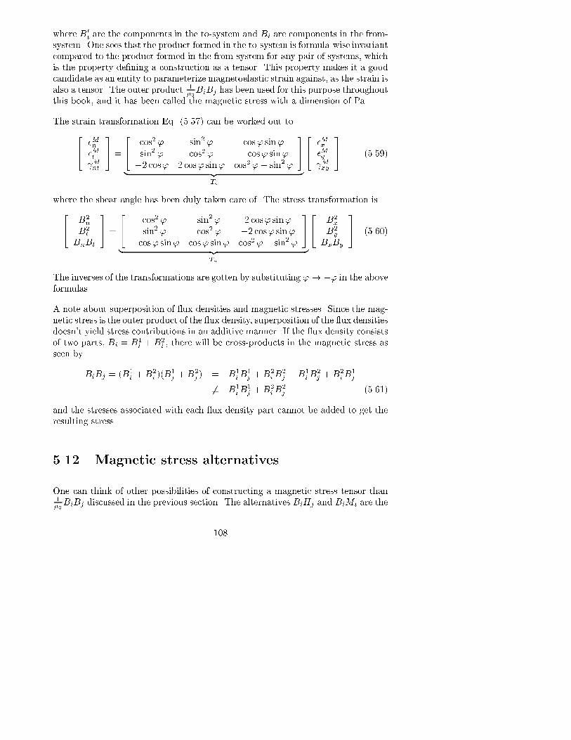
where B0i are the components in the to-system and Bi are components in the from-
system. One sees that the product formed in the to-system is formula-wise invariant
compared to the product formed in the from-system for any pair of systems, which
is the property de�ning a construction as a tensor. This property makes it a good
candidate as an entity to parameterize magnetoelastic strain against, as the strain is
also a tensor. The outer product 1�0BiBj has been used for this purpose throughout
this book, and it has been called the magnetic stress with a dimension of Pa.
The strain transformation Eq. (5.57) can be worked out to24 �Mn
�Mt Mnt
35 =
24 cos2 ' sin2 ' cos' sin'
sin2 ' cos2 ' � cos' sin'
�2 cos' 2 cos' sin' cos2 '� sin2 '
35
| {z }T�
24 �Mx
�My Mxy
35 (5.59)
where the shear angle has been duly taken care of. The stress transformation is24 B2
n
B2t
BnBt
35 =
24 cos2 ' sin2 ' 2 cos' sin'
sin2 ' cos2 ' �2 cos' sin'� cos' sin' cos' sin' cos2 '� sin2 '
35
| {z }T�
24 B2
x
B2y
BxBy
35 (5.60)
The inverses of the transformations are gotten by substituting '! �' in the above
formulas.
A note about superposition of ux densities and magnetic stresses. Since the mag-
netic stress is the outer product of the ux density, superposition of the ux densities
doesn't yield stress contributions in an additive manner. If the ux density consists
of two parts, Bi = B1i +B2
i , there will be cross-products in the magnetic stress as
seen by
BiBj = (B1i +B2
i )(B1j +B2
j ) = B1iB
1j +B2
iB2j +B1
i B2j +B2
iB1j
6� B1iB
1j +B2
iB2j (5.61)
and the stresses associated with each ux density part cannot be added to get the
resulting stress.
5.12 Magnetic stress alternatives
One can think of other possibilities of constructing a magnetic stress tensor than1�0BiBj discussed in the previous section. The alternatives BiHj and BiMi are the
108

ones most obvious. They have a magnetic material in uence built in, like Hk�ikHj .
It is possible to simplify BiMj to1�0BiBj when �rjk � 1 : j = k; �rjk = 0 : j 6= k
(large permeability without coupling between directions) as seen from the formula
Mj =1�0Bj�Hj . It is unknown how muchH really in uences. H is more connected
to the applied �eld from external coils and edges of the specimen. Inside the
material, B and M have very equal directions, due to the ferromagnetic material
property, and strain is believed to depend only on these internal entities. When
the external entity H is not codirected with M , it will probably only tend to rotate
the state of strain (when the sample is �xed) as it will rotate M . If this rotation
of strain will also be accompanied with a rotation of matter probably depends on
the type of magnetic material. For soft2materials the atomic moments perhaps
can rotate on the lattice sites and stay internally parallel, without rotation of lines
connecting lattice points. For hard materials, there are certain easy directions
in which the atomic magnetization vectors probably lie. Switching between these
directions occur when the applied �eld rotates. One can imagine that there can be
some rotation of lattice lines as the cells try to keep the magnetization in the initial
cell easy direction before switching occurs. The phenomenon might be consistent
with a torque action description. As the applied �eld rotates, the torque on cells
increases until the atomic moments turn relative the cells and the torque becomes
zero, or less than critical. To conclude, B and M might be adequate to describe
strain, while H has to be used when describing rotation. In an inhomogeneously
magnetized material, there will be local distortions of H , so the local H has to be
distinguished from the applied H .
When there is hysteresis between the magnetic stress and the resulting strain, it
would be interesting to keep track of both B and H during the hysteresis cycle.
There is a possibility that the hysteresis is purely magnetic, and that the con-
struction of a more proper magnetic stress tensor (perhaps BiHj) would lead to a
hysteresis-free magnetic stress-magnetoelastic strain relation.
5.13 Compliance transformation
It is appropriate to write out how to transform the magnetocompliance. By trans-
forming the stress in the xy-system to the nt-system, multiplying with the nt-system
compliance matrix Dnt to get the strain, and transforming the strain back to the
2Soft and hard in this context states the ease of rotation of magnetization. Normally, soft andhard states the ease of changing the sign of magnetization along an axis. These two qualitiesmight di�er.
109

xy-system, one can identify the xy-system compliance matrix Dxy,
�Mxy
= T�1� DntT�| {z }Dxy
�Mxy
(5.62)
where �Mxy
is the column of magnetic stress components in th xy-system, �Mxy
=1�0[B2
x; B2y ; BxBy]
T , and �Mxy
is the column of magnetostrictive strain components,
�Mxy
= [�Mx ; �My ; Mx y]T . For an anisotropic material, the compliance will depend
on the angle ' between the nt-coordinate system and the xy-system.
In the magnetoorthotropic case with the x,y-coordinate axes parallel to the char-
acteristic material axes, the compliance matrix is written
Dxy =
24 Dxx Dxy 0
Dxy Dyy 0
0 0 Dxyxy
35 (5.63)
with Dxx 6= Dyy. The orthotropic model doesn't always give a principal strain
system coincident with a principal stress system. The principal strain tends to be
rotated towards the easy material characteristic axis. Moreover, symmetry in the
compliance matrix means something for the contraction ratios between di�erent
directions. The application of stress in a hard characteristic direction will give a
higher strain ratio between easy and hard direction than the strain ratio between
hard and easy direction when the same magnitude of stress is applied to the easy
direction.
By transforming with Dnt = T�DxyT�1� one gets a full matrix for the nt-system,
Dnt =
24 Dnn Dnt Dnnt
Dnt Dtt Dtnt
Dnnt Dtnt Dntnt
35 (5.64)
where the entries are
Dnn = 1=8 cos4'Dxx + 1=2 cos2'Dxx + 3=8Dxx + 1=8Dxyxy
�1=8 cos4'Dxyxy � 1=2 cos2'Dyy + 1=8 cos4'Dyy + 3=8Dyy
�1=4 cos4'Dxy + 1=4Dxy (5.65)
Dnt = 1=8Dxx � 1=8 cos4'Dxx + 3=4Dxy + 1=4 cos4'Dxy
+1=8Dyy � 1=8 cos4'Dyy � 1=8Dxyxy + 1=8 cos 4'Dxyxy (5.66)
Dnnt = �1=4Dxx sin 4'� 1=2Dxx sin 2'+ 1=2Dxy sin 4'+ 1=2Dyy sin 2'
�1=4Dyy sin 4'+ 1=4Dxyxy sin 4' (5.67)
Dtt = 3=8Dxx � 1=2 cos2'Dxx + 1=8 cos4'Dxx + 1=4Dxy
�1=4 cos4'Dxy + 1=8 cos 4'Dyy + 1=2 cos 2'Dyy + 3=8Dyy
110

+1=8Dxyxy � 1=8 cos4'Dxyxy (5.68)
Dtnt = �1=2Dxx sin 2'+ 1=4Dxx sin 4'� 1=2Dxy sin 4'+ 1=4Dyy sin 4'
+1=2Dyy sin 2'� 1=4Dxyxy sin 4' (5.69)
Dntnt = 1=2Dxx � 1=2 cos4'Dxx �Dxy + cos 4'Dxy
+1=2Dyy � 1=2 cos4'Dyy + 1=2 cos4'Dxyxy + 1=2Dxyxy (5.70)
This compliance transformation can be used to �nd the axes of extremal compli-
ances to uniaxially applied stresses. A uniaxial stress can be written as
�Mnt
=
24 �M
0
0
35 (5.71)
where �M is a scalar, with the the nt-system chosen with the n-axis parallel to the
stress application axis. The strain response is then24 �Mn
�Mt Mnt
35 = Dnt
24 �M
0
0
35 =
24 Dnn(')
Dnt(')Dnnt(')
35�M (5.72)
Dnn(') is the compliance parallel to the application axis, it will be called the normalcompliance in the following. Dnt(') is the orthogonal compliance to the applicationaxis, and Dnnt is the shear compliance in the nt-system. By varying the angle of
application ', the extremals of the compliances can be searched. The extremals areeasily found for a model by plotting the functions 5.65, 5.66 and 5.67. Such plots
can be used to compare a model with strain measurements where uniaxial stresses
have been applied in di�erent directions. The plots for the values given in section
5.7 is given in Figs. 5.2, 5.3 and 5.4.
5.14 Piezomagnetism
The total dipole moment of a crystal may be changed by the movement of the
walls between domains or by the nucleation of new domains. Only walls separat-
ing domains with 90� domain magnetization direction di�erence will contribute to
magnetostriction with its motion.
The response of piezomagnetic crystals in transducer applications is characterized
by the magnetomechanical coupling factor k, de�ned by
k2 =energy convertible to mech:work
mag: energy stored(5.73)
111

Normal magnetocompliance [1/Pa]
4e-12
8e-12
1.2e-11
1.6e-11
2e-11
30
210
60
240
90
270
120
300
150
330
180 0-
+
-
+
Figure 5.2: Normal magnetoelastic compliance as function of angle of magnetic
stress to rolling direction.
Orthogonal magnetocompliance [1/Pa]
1e-11
2e-11
3e-11
4e-11
30
210
60
240
90
270
120
300
150
330
180 0+
-
+
-
Figure 5.3: Orthogonal (to magnetic stress) magnetoelastic compliance as function
of angle of magnetic stress to rolling direction.
112

Shear magnetocompliance [1/Pa]
1e-11
2e-11
3e-11
4e-11
30
210
60
240
90
270
120
300
150
330
180 0
+-
+ -
Figure 5.4: Shear magnetoelastic compliance coe�cients as function of angle of
magnetic wtress to rolling direction.
The constitutive relation between small-signal magnetic ux density B, stress �,magnetic �eld strength H and strain �
B = �H + d� (5.74)
� = dH + C� (5.75)
The piezomagnetic constant d is the same in both equations due to the idea of
reversibility, energy can ow equally well in both directions between electrical and
mechanical terminals. � is the permeability at constant stress and C is the elastic
compliance at constant magnetic �eld strength. For the coupling coe�cient to be
non-zero, the small-signal quantities have to be imposed on bias quantities.
The way they are written, Eqs. (5.74) and (5.75) are suitable for � and H as inde-
pendent variables. Another choice of independent variables gives another (equiv-
alent) material relation. When analyzing the conversion of energy through the
material, B and H can be chosen as independent variables. By exciting the sample
with a small-signal B at constant stress (zero small-signal stress), the magnetic
energy density stored will be B2=2��. By mechanically loading the sample at con-stant B, a decrease of magnetic energy follows. The magnetic energy di�erence
113

is converted to stored mechanical energy. By closing the small-signal B �H loop
with a decrease of B at constant strain, we know from the symmetry of the trans-
duction matrix that the enclosed B �H loop area has been actually transferred to
mechanical work. The loop area divided by the �rst phase magnetic storage gives
the expression for k2 = (�� � ��)=�� , or k2 = d2=�C by using the transduction
coe�cents in Eqs. (5.74) and 5.75. �� and �� are the permeabilities at constantstress and constant strain, respectively.
5.15 Physical models
The phenomenon of magnetostriction is the ability of pieces of ferromagnetic ma-
terials to elongate or contract by the presence of a magnetic �eld. The sponta-
neous magnetostriction of a Weiss domain is obtained as the material becomes
ferromagnetic by cooling below the Curie temperature. Curie temperatures for
the three principal ferromagnetic elements are several hundred degrees centigrade,
which means that spontaneous magnetostriction in these elements and their com-
mon alloys is present at room temperature. What we will mean by magnetostriction
in the following is the observed elongation of an initially unmagnetized piece as a
result of an applied magnetic �eld. This occurs as magnetic domain magnetiza-
tion vectors are oriented from a pseudo-random con�guration at zero applied �eld
strength to a con�guration with a resultant macroscopic magnetization by the ex-
ternal application of a magnetic �eld strength. In the following, by magnetization
we mean, if not otherwise stated, the macroscopic quantity observed as a spatial
average of domain magnetizations. Of course, for this to be a relevant description of
the magnetic response, the object under consideration has to contain a large num-
ber of domains initially (the perfectly saturated magnetic state is a single domain)
. If the specimen is a single-crystal, this would probably mean that a large number
of impurities or lattice defects has to be present, otherwise domain wall motion
would be uninhibited and single domain behaviour would easily be achieved. Strict
single domain behavior is associated with domain rotation between magnetically
easy directions in the lattice and the in uence of the so called form-e�ect from the
discontinuous change of magnetization at the edges of the specimen.
The principal elements are Cobalt, Nickel and Iron, and alloys of interest to us are
Silicon-Iron (SiFe), Cobalt-Iron (CoFe), Nickel-Iron (NiFe) and Terfenol-D (TbFeDy).
Applications include power transformer cores and ux conductors in large electric
power generators (oriented SiFe), electric motors (unoriented SiFe), relays (NiFe),
ultrasonic transducers (CoFe), actuators for prospecting, shaking and vibration
control (TbFeDy).
114

RDTD
001
010
100
Figure 5.5: (110)[001] crystal orientation. RD is rolling direction and TD is trans-
verse direction of the sheet.
5.16 Material structure
5.16.1 Texture
Texture is the important structure property here. Since all the rolled materials
are polycrystalline, there can be a structure of the alignment of the crystallites
that make up the body. That structure is called the texture of the material. In
NO (non-oriented) materials, there is no preferred direction and the material will
supposedly be isotropic. In GO (grain oriented) materials there will be a distinct
preferential direction close to the rolling direction. Furthermore, the crystal unit
cube is characteristically rotated around the preferential direction. Two rotational
positions are encountered, the cube-on-face variant and the cube-on-edge position.
The latter is the common texture for GO SiFe.
The three polycrystalline textures are (110)[001], (100)[001] and nonoriented (with
grains randomly oriented). The (110)[001] texture has the unit cell cube of the
grain crystals oriented with the cube diagonal plane (110) parallel to the rolling
plane and the cube edge [001] parallel to the rolling direction, see Fig. 5.5 The
production of such textured SiFe material was invented by Goss in 1933 and the
texture is frequently named after him. The name is "cube-on-edge" which is short,
but imprecise since the rotation of the cube around the edge is unspeci�ed. The
(100)[001]-texture is called "cube-on-face" since the cube face is parallel to the
rolling plane, but to be exact one has to add that the cube edge is parallel to the
rolling direction.
115

5.16.2 Transformer iron qualities
The commercial grades of grain oriented silicon iron sheet are
� CGO, conventional grain oriented, (Mx, e.g. M5, are American AISI standard
names).
� HIB, "high B", superoriented material, (no independent standard).
� Material improved during last couple of years.
The di�erences between the classes of materials lie in the mean deviation �� of the
misalignment angle � between the grains in the sheet to the rolling direction of the
sheet. The grain direction is taken as the direction of the cube edge of the crystal,
which is also a direction of easy magnetization.
The directional magnetic properties of a sheet with Goss texture comes from the
fact that the cube edges are directions of easy magnetization of the SiFe crystal. The
rolling direction (RD) is very close to an easily magnetized direction of the crystals
and is therefore used in the longitudinal direction of limbs and yokes in a core. The
transverse direction (TD), where transverse is with respect to rolling direction, is
on a cube face diagonal, which is not an easy direction of the crystal, resulting in a
much lower directional permeability than �RD. In between RD and TD one �nds
the hardest direction (HD) on the cube diagonal, which is at atan(p2) = 54:7�
from RD.
5.17 Micromagnetic cause of magnetostriction
The magnetostrictive strain is a relative displacement of the lattice planes, a change
of the lattice parameter, due to ux density change. The ux density changes the
equilibrium con�guration of lattice planes in the quantum-mechanical system of the
crystals.
It might be possible to solve for quantum-mechanical equilibrium by stating a
cell problem which is de�ned on the basis unit of the crystal. The Schr�odinger
equation would then be solved numerically with the appropriate periodic boundary
conditions. That kind of simulations are performed in the area of materials science.
To get the e�ect of the complete medium, a homogenization could follow such a
calculation to get the macroscopic magnetostriction to ux density relation.
116

Another possibility is to solve with so called micromagnetic simulation: A set of
interaction relations between the lattice points is stated and is simulated in time
with an externally applied �eld. Such interaction relations for purely magnetic
response have been formulated and go under the names of Ising (nearest-neighbour
interaction) and mean-�eld interaction.
A di�culty with both the cell problem and the micromagnetic formulation is how
to model grain boundaries. Those surfaces are sources of disturbances as well as
sites of impediment. Disturbances in this case are the nucleation of domains, and
impediment is pinning and release of domain walls.
5.18 Domains in soft magnetic materials
Power losses and acoustic noise are due to
� domain wall pinning
� domain nucleation/formation
� domain annihilation
� domain magnetization rotation
Domains occur as an answer to the global energy minimization principle. Phenom-
ena on many levels contribute to the energy:
� stray �eld energy
� anisotropy energy
� exchange energy
� magnetoelastic energy
� external �eld energy
The stray �eld energy is most important, since large amounts of energy can be saved
by keeping the ux inside the material. This phenomena is a balance between the
possibility of getting a lower H �eld inside the material than in the air, and the
possibility of getting a lower B �eld by spreading out the ux in the air. Minimizing
stray �eld only in an isotropic material would not give rise to domains but ux
117
lines would be smooth and only re ect the specimen shape in order to achieve ux
closure with optimal spreading out of ux. In an anisotropic material there could
be something resembling domains, since the ux lines would have kinks in going
from one preferred direction to another.
Anisotropy energy is linked with the magnetization in a single crystal, where there
will be directions di�cult to magnetize and others easy to magnetize, dependent on
the distribution of atomic sites and the interaction between atomic magnetizations.
Exchange is the underlying quantum-mechanical phenomenon of ferromagnetism.
There will be a non-classical contribution to the magnetic energy from interchange
of spin between atomic sites in a pair of atoms. This contribution can lead to a
favourable energy situation when spins are parallel, which occurs in ferromagnetic
substances.
Magnetoelastic energy enters as there is probably always at least a weak coupling
between magnetic �eld and strain �eld. The phenomenon can be analyzed on two
di�erent levels: lattice level and macroscopic level. On the lattice level, one could
make a cell problem and solve the Schr�odinger equation with variable lattice param-
eter and magnetic ux density, and see how the lattice would expand or contract
as magnetic �eld was changed. On a macroscopic level, it is possible to introduce
coupling parameters between the pure mechanical entities and the pure magnetic
entities. Stratton made suggestions for such parameterizations regarding the elec-
tromechanical case for dielectrics. Linearized material relations are used for biased
signals in piezoelectric and magnetostrictive (a.k.a piezomagnetic) transducers.
The grain size is important in a magnetic context, since very small grains might
become single domain particles as demagnization e�ects from the boundary of the
grain will take over, a phenomenon used to make permanent magnets. In soft
magnetic materials, the grain boundaries will act as pinning sites to the moving
domain walls during dynamic excitation, and the grain size and shape will a�ect
power lost to the lattice through these sites.
Misorientation of an easy axis to a specimen surface will a�ect the domain pattern
viewed on the surface. In SiFe with a perfect orientation of a (100) surface, the
pattern viewed in the middle of the plane should be broad stripe domains at low H-
�elds and narrow stripe domains at high H-�elds. Close to the edges of the surface
there will be triangular domains providing ux closure between the stripes, as neigh-
bouring stripes have opposite magnetization directions. On a slightly misoriented
surface, s.c. supplementary domains will occur, forming a tree pattern with spiky
branches extending from the wall separating the main stripe domains. There could
also appear a lancet-shaped supplementary pattern, with spikes oriented along the
stripes and scattered over the stripes. Loss and noise doesn't simply depend on do-
main wall movement, the reorganization of domain structure (including appearance
118

and disappearance of domains) will also come into the picture.
5.19 Domain walls and magnetostriction
Domain walls are named after the di�erence in magnetization direction between
the domains divided by the wall. Between stripe domains there are 180� walls andbetween closure domains and stripe domains there are 90� walls.
In every domain M is constant, equal to the bulk saturation magnetization achiev-
able with ordinary equipment ("technical saturation"). If the walls present in the
specimen were only of 180� type and the motion of the walls was perpendicular to a�xed direction (possibly the excitation direction) there wouldn't be any noticeable
magnetostriction, because domain magnetostrictive strain would be of same magni-
tude and state regardless of the motion of the domain walls. In a real sample there
will be closure domains at the edges and surfaces (at least for a soft magnetic mate-
rial) and there might be wall irregularities, domain nucleation processes or closure
domains at grain boundaries. For samples with poor grain alignment, there will
be deviation of domain magnetization direction between neighbouring grains when
domains try to span multiple grains. The microscopic strain is therefore position-
and applied �eld strength-dependent even during uniaxial excitation, leading to a
changing macroscopic strain during the excitation cycle. For well-aligned cube-on-
edge materials, the negative magnetostriction in the rolling direction is attributable
to spike domains (also called lancets) observable on the sample surface, as under-
stood by Shur (1947). The lancets occur due to misalignment of a grain easy axis
with sheet surface, and provide ux closure for the stray �eld caused by the mis-
alignment. This closure is achieved by a volume domain directed from one surface
of the sheet to the other, parallel to the normal of the sheet and at ninety degrees
to the main domains. The dynamics of the associated ninety degree walls will lead
to an observable magnetostriction. Due to the unknown details and quantities of
the processes leading to a non-constant strain, it is hard to �nd a mathematically
accurate �eld strength to strain expression directly from physical reasoning.
What one can say is that the strain is equal for opposite signs of applied �eld
strength at opposite signs of �eld strength time derivative (strain at equal amount
of reversal from saturation is independent of sign of bulk magnetization). An even
form of the anhysteretic magnetostriction curve can then be postulated. A higher
density change of 180� domain walls during the cycle will lead to a higher degree ofnon-180� wall activity, leading to a higher magnetostriction valley-to-peak value.
Therefore the maximum wall density comes in when predicting the strain magni-
tude, together with kind of material (saturation magnetostriction value and degree
of grain alignment) and individual sample dependency (spread due to manufactur-
119
ing process or handling).
5.20 Domain types
The domain types are band(or stripe)-patterns, spike(or lancet)-domains, and maze-
patterns. On Goss textured SiFe-sheet surfaces with a grain easy axis nearly parallel
to the surface the primary domain structure seen is a stripe pattern (the primary
structure) and the secondary, smaller, structure is a spike-pattern, see Fig. 5.6.
The spike-domains occur at grain interfaces and at grain surfaces. Maze patterns
occur on unpolished surfaces.
At grain interfaces spike-domains result from the misalignment of neighbouring
grain easy axes, by the fact that the magnetization component normal to the in-
terface is discontinuous and sources an increased magnetic stray �eld, a �eld that
is decreased by the introduction of spike domains. The domains provide a path for
some ux to close within the material, which is energetically favourable compared
to closing the path through air. The same reason holds for spike domains that can
occur along domain walls separating stripe domains for (100)[001]-textured sheet.
In this case, the magnetization discontinuity occurs due to the grain easy axis mis-
alignment with the sheet surface, and the observable pattern is a tree-like array of
spikes, each of which is like a small magnet needle, bent at the middle. The grain
misalignment with sheet surface sources spike domains scattered over the stripe
domains for (110)[001]-textured sheet as stated above.
There is a correlation between grain length and domain width. In grain-oriented
(commonly Goss textured) silicon-iron, the grains are about 25 mm long and the
domains are roughly 0.5 mm wide. If the grains are made longer, the domains
will be wider (perpendicularly to the grain length dimension). This is due to the
fact that the angle between the grain boundary and the transverse direction will be
lower after the grain size has been increased, which reportedly lowers magnetization
discontinuity between grains. The domains can then a�ord to get wide and escape
the energy needed to create domain walls. The wider domains will increase stray
�eld at interfaces because the equivalent N and S poles will in the mean be farther
away from each other, but walls occur across grains and not only at interfaces. The
resulting domain width balances the two energy contributions.
There is also a correlation between losses and domain width. The local eddy current
losses will decrease with lower domain width, indicating that a material with a �ne
domain structure should be chosen for transformer and machine applications. But
a low domain width is also a sign of high interfacial discontinuity, that will be
accompanied by spike domains. Spike domains will source much larger losses than
120

z
Figure 5.6: Main stripe domains with supplementary lancet domains.
Figure 5.7: Lancet domain viewed from the side.
121

the primary domain structure, leading to a minimum loss at a grain length of about
0.5 mm, which balances domain �neness and lack of spike domains.
There are simple models that predict positive magnetostriction in the rolling direc-
tion of SiFe sheets, as an e�ect of domain magnetization directional changes from
other easy axes to the easy axis parallel to the rolling direction. In (110)[100]-
textured sheet, most domain magnetizations are already [100] or [�100] in the de-
magnetized state, so the e�ect is very small. Empirically, negative magnetostriction
up to �2�m=m is found. Allia explained the unexpected behaviour by formation
of volume domains in the body of the sheet having 90� walls, occuring due to grainmisalignment with sheet surface. These volume domains are connected to surface
spike or lancet domains described above. The spike domains vanish at a critical
�eld and the magnetostriction becomes less negative as the �eld is increased.
Nonoriented sheet has a large (up to 40�m/m) positive magnetostriction due to
alignment to [100] magnetizations from a wider distribution of [010] and [001] mag-
netizations. By applying a tension one can introduce an anisotropy in this sense
and make the demagnetized state contain more [100] domains. Then the negative
magnetostriction contribution from spike domains can be seen again.
122

Chapter 6
Magnetic �nite element
analysis
6.1 Introduction
Simulations are interesting in two respects. Firstly, the measurement setup (yokes,
sample and sample table) can be analyzed. Such analysis was carried out to eval-
uate the concept before the setup was built, later to investigate the magnetic and
magnetoelastic �elds in the sample with a material model hypothesis. Also an error
source, bending of the sample, was analyzed by simulation. The second respect is
that to be of greater engineering use, material models obtained from hypothesis
and experimentation should be stated in such a form to allow them be included in
simulation programs. That is why the study of the simulation method, at least to
some level, is important to the experimenting researcher. The project which made
this book as an o�spring even had as an ultimate research goal to parameterize the
phenomenons encountered, so greater weight has been put on the aspect here.
When studying di�erent alternatives of software to buy, it was soon clear that
none of them really allowed the user to experiment with unconventional, nonlinear
and/or frequency- dependent material models. At the time of evaluation only lin-
ear or splined magnetic material functions could be entered, and magneto- elastic
formulations, if at all present, was only for small-signal linearized behaviour. It
was decided to write the programs by own hand, and the MATLAB language and
interpreter was chosen to get full control over formulation and material models,
while still providing a decent solver to the �nal equation system, so hand coding of
123

or library search for such a solver was avoided. MATLAB's pretty plotting facilities
also charmed the author.
The simulation technique for the cases presented in this book is the �nite element
method, and the variants used will be presented in some detail. First a program
to calculate the magnetostatic two dimensional magnetic excitation of the sample
was written.
Of special interest are the results concerning the area of uniform magnetic and
mechanical �elds where sensors are placed.
An in-house 3D program has also been used. One can de�ne geometry and carry
out calculations on rectangular parallelepiped elements (also called brick elements).
The program was written in C and is for magnetostatic approximations. Trilinear
basis functions to the magnetic scalar potential are used and a linear anisotropic
magnetic material relation (� a constant tensor) is used as material model. The
crossed yokes of C-core shape with the by them fed sample has been geometrically
described. Coils on the yokes have been modelled by equivalent surface poles.
6.2 Coupling
There is a magnetomechanical problem because the constitutive relation �(�;BiBj)
is valid over a continuum with boundary conditions and ~B not homogeneous, i.e � isnot directly achieved from ~B due to elastic interaction. The coupling can be written
as B ! �$ �. There is a weak coupling between � and �, and the additional smalldeformation approximation make it possible to solve the magnetic problem �rst,
followed by a mechanical simulation. The simulations are thus decoupled. Eddy
currents are neglected due to the sheets used being thin and with a relatively high
resistivity. A magnetostatic analysis will therefore do.
6.3 General motivation and conditions for simula-
tions with computer
Problem: How predict a vibration level/noise level from a conceived design change
? Experiments and small scale prototype manufacture can be expensive or mislead-
ing, and full scale experiments are impossible in many cases.
Solution: A good characterization, magnetic and magnetostrictive, of the core ma-
terial, with �tting software for computer simulations. The software should thus be
124
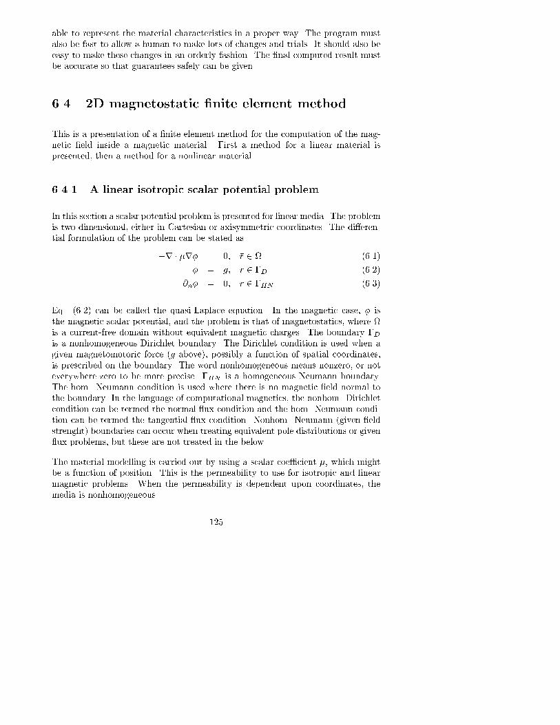
able to represent the material characteristics in a proper way. The program must
also be fast to allow a human to make lots of changes and trials. It should also be
easy to make these changes in an orderly fashion. The �nal computed result must
be accurate so that guarantees safely can be given.
6.4 2D magnetostatic �nite element method
This is a presentation of a �nite element method for the computation of the mag-
netic �eld inside a magnetic material. First a method for a linear material is
presented, then a method for a nonlinear material.
6.4.1 A linear isotropic scalar potential problem
In this section a scalar potential problem is presented for linear media. The problem
is two-dimensional, either in Cartesian or axisymmetric coordinates. The di�eren-
tial formulation of the problem can be stated as
�r � �r� = 0; �r 2 (6.1)
� = g; �r 2 �D (6.2)
@n� = 0; �r 2 �HN (6.3)
Eq. (6.2) can be called the quasi-Laplace equation. In the magnetic case, � is
the magnetic scalar potential, and the problem is that of magnetostatics, where
is a current-free domain without equivalent magnetic charges. The boundary �Dis a nonhomogeneous Dirichlet boundary. The Dirichlet condition is used when a
given magnetomotoric force (g above), possibly a function of spatial coordinates,
is prescribed on the boundary. The word nonhomogeneous means nonzero, or not
everywhere zero to be more precise. �HN is a homogeneous Neumann boundary.
The hom. Neumann condition is used where there is no magnetic �eld normal to
the boundary. In the language of computational magnetics, the nonhom. Dirichlet
condition can be termed the normal ux condition and the hom. Neumann condi-
tion can be termed the tangential ux condition. Nonhom. Neumann (given �eld
strenght) boundaries can occur when treating equivalent pole distributions or given
ux problems, but these are not treated in the below.
The material modelling is carried out by using a scalar coe�cient �, which might
be a function of position. This is the permeability to use for isotropic and linear
magnetic problems. When the permeability is dependent upon coordinates, the
media is nonhomogeneous.
125

6.4.2 Discretization
The �nite element method provides a scheme to obtain a discretized, approximate,
version of the space continuous problem. The approximate problem has a solution
that is also de�ned at every point in space, but is only determined by a �nite num-
ber of (discrete) values. The global domain is subdivided into elements, and over
each local element, the approximate solution is chosen with a simple (polynomial)
form. The values of the approximant (or derivatives of it) at the vertices of the
elements (or some other discrete nodes) will determine the approximate solution.
Those values are called degrees of freedom (dofs). The dofs are determined by min-
imization of the energy of the approximant. To conclude, the local approximant
form will together with energy integrals �tting the di�erential equation give the
best approximate solution possible for the form choice.
In the case of a linear local approximation (piecewise linear globally), the solution
has to be sought of the potentials in the nodes where no Dirichlet boundary con-
dition is imposed. These nodes will be called active nodes in the following, and
consist of inner nodes as well as Neumann boundary nodes. Furthermore, if the
equation is linear, i.e. if the permeability does not have any dependency upon the
potential (or any derivative thereof), the discretization leads to a system of linear
equations, which will be described in the following.
A good approximate solution will satisfy the integrated weighted di�erential equa-
tion for many weighting functions. By using integration by parts, one can transfer
one di�erentiation of the solution to the weight function, and allow approximants
with less regular behavior to be solutions.
�Z
wr � �rphid = �Z�
w�r�~nd� +
Z
rw � �r�d = 0 (6.4)
w is the weight function. By writing the solution as a linear combination of simple
basis functions Ni (Ni e.g. piecewise linear in x; y) and choosing the weight func-
tions as the basis functions, one gets the Galerkin formulation of the problem. It is
a well known fact [103] that the Galerkin solution function is orthogonal to the true
solution function and that the error function thereby is minimized in energy norm.
The Galerkin solution u(x; y) =P
iNi(x; y)ui can be determined by integrating
and solving
�Z�
Nj�Xi
rNiui~nd� +
Z
rNj � �Xi
rNiuid = 0 (6.5)
for all combinations of basis function indices i; j. If the elements are triangular andthe basis functions are piecewise linear, continuous, and nonzero in only one node
with index equal to basis function index, the element parts of the integration can
be carried out with help from the next section.
126

The basis functions to the global problem only have a small localized support, and
the support of a gradient of a given basis function will only overlap with a small
number of other basis function gradient supports, so the resulting equation system
matrix is sparse.
6.4.3 Single triangle element
When using a linear approximant over a triangular element that has its vertices
as nodes, it can be observed that the values of the linear approximant that is
unity in one node and zero in the other two, will constitute a kind of coordinate of
the distance normally to the baseline between the zero nodes. By permuting the
unity node and the baseline, another coordinate is gotten, and the two coordinates
can be used to specify a point location. By permuting once more, a redundant
third coordinate is gotten. These three coordinates are called the area coordinates
N1; N2; N3 and are equal to three simple linear approximants (shape functions) that
make up the total element approximant by superposition.
The area coordinates Ni, i = 1; 2; 3, are24 N1
N2
N3
35 =
1
2A
24 x2y3 � x3y2 y2 � y3 x3 � x2
x3y1 � x1y2 y3 � y1 x1 � x3x1y2 � x2y1 y1 � y2 x2 � x1
3524 1
xy
35 (6.6)
where xi; yi; i = 1; 2; 3 are the coordinates of the vertices of the triangle. To
remember the structure of the formula one can notice how the indices permute.
One should also note that the area coordinates are linearly dependent. The use of
this choice is evident if one explores the property
Ni(�rj) = �ij ; i; j = 1; 2; 3 (6.7)
i.e the i:th area coordinate is equal to unity in the i:th vertex of the triangle and
is equal to zero in the two other vertices, and according to the transformation
above the coordinate varies linearly in between the vertices. Thus, an arbitrary
linear function over the triangle can be decomposed into a superposition of area
coordinates. In the above equations, A is the area of the triangle,
A =1
2f(x2 � x1)(y3 � y1)� (y2 � y1)(x3 � x1)g (6.8)
The gradients of the area coordinates will be of further use,
rNi =1
2A(yj � yk; xk � xj); i = 1; 2; 3; j = i� 1; k = i� 2 (6.9)
127

where � is the modulo 3 addition operator1 . Note that the gradients of Ni are
constant vectors. The direction of the i:th gradient is normal to the line connectingthe vertices number i�1 and i�2. One is now able to construct a symmetric matrix
s of scalar products between the area coordinate gradients de�ned by a triangle,
sij = 4A2rNi � rNj (6.10)
s11 = (y2 � y3)2 + (x3 � x2)
2 (6.11)
s21 = (y3 � y1)(y2 � y3) + (x1 � x3)(x3 � x2) (6.12)
s22 = (y3 � y1)2 + (x1 � x3)
2 (6.13)
s31 = (y1 � y2)(y2 � y3) + (x2 � x1)(x3 � x2) (6.14)
s32 = (y1 � y2)(y3 � y1) + (x2 � x1)(x1 � x3) (6.15)
s33 = (y1 � y2)2 + (x2 � x1)
2 (6.16)
This matrix contains biquadratic terms of the coordinates of the vertices of the
triangle and will be used in the FEM algorithm. By multiplying s with the perme-
ability � and a coordinate system scale factor h (h = r for axisymmetric coordinatesr,z) and then integrating over the triangle, one gets the so called local sti�ness (or
system) matrix for the triangle.
6.4.4 System of linear equations
Proceeding with the practical handling of the discretized problem, one can study
the case of what can be called an undetermined system - the matrix problem cor-
responding to a di�erential equation with homogeneous Neumann conditions on all
boundaries. As will be seen later on, the undetermined system is the discretized
problem without boundary conditions imposed. Algorithmically it is simpler to set
up the undetermined system �rst and then impose constraints from the Dirichlet
nodes. By writing the undetermined problem
u =X
j2A[DNjuj (6.17)
Sij =
Z
rNi � �rNjhd i; j 2 A [D (6.18)
S�u = 0 (6.19)
where u = u(x; y) is the approximate solution �eld, �u is the column of nodal values
of u, A are active nodes (inner nodes + Neumann boundary nodes), D are Dirichlet
1The modulo 3 addition counts with wraparound. If counting would begin with 0, wraparoundto 0 would occur at 3, normally counted. In this text, counting begins with 1 and wraparoundoccurs at 4, e.g 3� 1 = 1, 2� 3 = 2.
128

nodes and S is the undetermined system matrix. It is clear that S is singular and
that there are in�nitely many solutions �u - a not properly posed problem, linked to
the notion of a oating potential. To make it properly posed, constraints from the
known Dirichlet nodes uj ; j 2 D are imposed by
fi =
� �Pj2D Sijuj i 2 A
ui i 2 D(6.20)
Sij =
�Sij i; j 2 A�ij otherwise
(6.21)
S�u = �f (6.22)
where �f is the excitation column, where an entry fi comes from Dirichlet nodes
surrounding node i. The Dirichlet nodes can be stored in the same column as the
active nodes, and the construction of the system matrix S and the contribution from
the boundary to the excitation column �f can be carried out in a single process, the
so called assembly. This process will be described below.
The assembly is regarded as building up the undetermined system matrix S by
summing contributions from each triangle Km. A single contribution, the local
system matrix s(m), is formed by integrating the gradient scalar product matrix
s(m), where m is the number of the triangle in question. Concisely,
Sij =Xm
s(m)ij (6.23)
s(m)ij =
ZKm
rNi � �rNjhd =
1
4A2s(m)ij �(m)
�A h = 113(x1 + x2 + x3)2� h = x
(6.24)
where d = dxdy and h = 1 when x; y are Cartesian coordianates and h = x when
x; y are axisymmetric coordinates (=r; z). Note that on the right side of Eq. (6.24),mu has been taken out of the integration and the formula is therefore strictly valid
only for a piecewise constant permeability.
6.4.5 Hollow cylinder test case
This test case was made to show the order of accuracy to expect from the method for
a certain mesh density. The case is obtained by solving Eq. (6.2) in axisymmetric
coordinates with z = 1 and z = 13 as homogeneous Neumann boundaries and r = 1
and r = 13 as Dirichlet boundaries, with a potential of 1 At assigned to the inner
side and 0 At assigned to the outer side. The mesh used was a triangulation with
a 13� 13 grid of nodes.
129

When comparing the numerical results to the analytical solution (a decaying log-
arithmic potential), one could see that in actual nodes the error is typically 1:3 %and in between nodes the error can reach 1:9 %. One should note that the error
considered is the potential error. Often in these kinds of �eld problems one is more
interested in the negative gradient of the potential (the magnetic �eld intensityH in
this case). By using a piecewise linear approximation of the potential , the �H-�eld
is piecewise constant and therefore probably more prone to errors. One must also
consider the e�ect of such an approximation when it comes to the ful�llment of the
interface conditions (continuity of normal ux density and continuity of tangential
magnetic �eld intensity), which is by no means guaranteed.
6.4.6 A nonlinear isotropic formalism
The nonlinear isotropic magnetic scalar potential problem consists of a scalar per-
meability dependent on the negative potential gradient, i.e. the magnetic �eld
intensity. The formal discretization scheme is the same as for the linear case, but
the end product is a set of simultaneous nonlinear equations. These equations can
be solved by iterative methods such as successive approximation (Chord method) or
successive linearization (Newton-Raphson method) or optimization methods such
as conjugate gradient methods (especially the incomplete Cholesky preconditioned
conjugate gradient method, the ICCG) or simplex methods. In the following, the
Newton-Raphson scheme will be adopted.
The N-R technique is outlined as follows.
�nd starting approximation �u(0)n = 0
while stop criteria not ful�lled
form residual ri(�un) = S(�un)ijuj � fi
form jacobian Pij(�un) = @ri
@uj
solve for Newton correction ��un = P�1�r(�un)form approximation �un+1 = �un +��un
n = n+ 1
(6.25)
In this scheme there are a number of things to clarify. First of all, the solution
vector contains all node variables regardless of type, so one will have to extend the
jacobian with trivial entries so that the Dirichlet node values will not be altered
during the iteration. The jacobian depends on all node values so that matrix will
have to be reassembled in each iteration. The fact that we are using piecewise
linear approximation here, will lead to a fairly simple expression of the jacobian as
an outer product of a single vector. Lastly, the stop criteria for the iteration has
to be stated. It is important here to remember to check not only the solution, but
130

also the residual, so the residual itself also has to be assembled in each iteration.
First, though, we have to express the residual and the jacobian. The residual is
ri ji2A =Xj2A
Sijuj � fi =X
j2A[D
Z
rNi � �rNjhduj =X
j2A[DSijuj(6.26)
ri ji2D = 0 (6.27)
Note that the residual is de�ned as zero for the Dirichlet nodes, while a multipli-
cation of the undetermined system matrix with the solution vector not necessarily
will produce zeroes in the Dirichlet node positions. The reason for introducing the
undetermined system matrix is once again because of its suitability for assembly.
The jacobian is a bit more elaborative to express. The de�nition is easily expanded
as
Pik =@ri@uk
=X
j2A[DfSij @uj
@uk+ (
@
@ukSij)ujg = Sik +
Xj2A[D
(@
@ukSij)uj 8i; k 2 A
(6.28)
since@uj@uk
= �ik. The second term is now examined. The derivative of a matrix
element is@
@ukSij =
Z
rNi � @�@uk
rNjhd (6.29)
and it is clear that it is only a�ected by a nonlinear �. The desired dependency
to express the permeability in is customarily, and probably the most convenient,
the magnetic �eld intensity squared. This is useful when isotropic materials are
present, since the directional properties of the �eld is not of interest. One should
also remember that a change in a single nodal variable changes the global �eld,
let alone with a small local support as the basis functions are constructed as such.
Writing the �eld and the nodal variable derivative thereof,
~H = �X
l2A[DrNlul (6.30)
@ ~H
@uk= �rNk (6.31)
one obtains a mathematical statement of that. Now, it is possible to write down
the nodal variable derivative of the permeability,
@�
@uk=
@( ~H � ~H)
@uk
@�
@H2= 2 ~H � @
~H
@uk
@�
@H2= 2
Xl2A[D
rNk � rNlul@�
@H2(6.32)
Thus, for linear triangular FEM it is seen that the derivative depends on the nodal
values in the vertices of adjacent triangles to the node in question, as well as
131

the permeability vs H squared, which is a function of the triangle number as the
�eld approximation is piecewise constant. Rewriting the second term suitable for
assembly one obtains Pj2A[D(
@@uk
Sij)uj =Pm 2 @�
@H2 jH2(Km)(RKm
hd)P
l;j2A[D ul[rNl � rNk rNi � rNj ]Kmuj (6.33)
where Km denotes the triangle with number m. For a given m only those i; k; l; jthat correspond to vertices on Km will contribute to the second term. By intro-
ducing the vector
bk = ~H � @~H
@uk=
Xl2A[D
ulrNl � rNk (6.34)
the assembly is somewhat simpli�ed, when evaluating this vector on the triangle
Km as
b(m)
k =X
l:~rl2Km
ul[rNl � rNk]Km=
Xl:~rl2Km
1
4A2s(m)
kl ul (6.35)
and writing a factor of the second term of the jacobian as an outer product of the
evaluated b-vector,
b(m)
k b(m)i =
Xl;j2A[D
ul[rNl � rNk rNi � rNj ]Kmuj (6.36)
Recall that local vectors and matrices superscripted by m only have nonzero entries
for indices corresponding to vertices on triangle Km and the storage is therefore
restricted to these. One can also notice that the H-�eld squared can be expressed
in terms of the b-vector,
H2(~r 2 Km) = (X
j:~rj2Km
rNjuj)2 =
Xi:~ri2Km
uib(m)i (6.37)
which is obtained after rewriting the square of the sum as a quadratic form of the
s(m)-matrix.
Another thing to sort out is how to de�ne the jacobian for entries that correspond
to Dirichlet nodes, when the equation
�r(�un) = P��un (6.38)
is solved for the Newton-Raphson correction ��un. Prior to solving this equation,
the residual elements corresponding to Dirichlet nodes, i.e. ri; i 2 D, are put
to zero. Now setting Pik ; i 2 D to �ik will produce zeroes in the Dirichlet node
elements of the Newton correction. This can be seen as extending the equation set
for the active nodes with trivial equations for the Dirichlet nodes. The equations
132

for the active nodes should remain unchanged, so Pik; i 2 A; k 2 D have to be set
to zero.
The stop criterion also have to be stated. It is immediately clear that the Euclidean
norm of the Newton correction should be close to zero, and this is often expressed
in a sense thatk��unkk�unk < tol (6.39)
The residual also has to be close to zero, inferring that
k��rnkk�rnk < tol (6.40)
In the case that �un = 0 is a possible iterate, the norm of the iterate may be safely
swapped to unity in the test. The tolerance tol is chosen according to the sought
accuracy, after the machine precision has been taken into account. When using
double precision, something like 10�5 might be considered.
6.5 3D isotropic formulation
To estimate the magnitude and homogeneity of the produced magnetic �eld in
the measurement area, three{dimensional magnetostatic �nite element simulations
have been performed using the following formulation. The relevant equations are
r� ~H = ~J; r � ~B = 0; ~B = � ~H (6.41)
The problem can be expressed on the form
~H = ~Hp �r�; r � (�r�) = r � (� ~Hp) (6.42)
where � is a continuous single{valued scalar potential used in the entire solution
region and ~Hp is any arbitrary vector �eld satisfying r � ~Hp = ~J [72]. A general
solution that is particularly convenient here is ~Hp =R( ~J � ~ex) dx, where ~ex is the
unit vector in the x{direction. Apart from being simple, an attractive feature of this
choice of ~Hp is that for the present geometry, it becomes zero everywhere except in
the regions contained within the coils. As a result, we avoid the cancellation error
e�ect in the test sheet which occurs when j ~Hpj � j ~H j. The term r � (� ~Hp) is a
surface density at the coil ends.
Fig. 7.1 shows results when a current was applied to one coil pair only. The sheet
had a size of 140�140�0:5 mm3 and a constant isotropic permeability � = 1000�0.The linear B �H relation adopted is appropriate for lower �eld intensities and is
133

su�cient to investigate homogeneity close to saturation. The system was solved
using 7168 trilinear block elements. The inhomogeneity of the magnetic �eld in the
central 60� 60 mm2 area was found to be approximately 10 %, while the leakage
ux was about 25 %.
6.6 3D anisotropic formulation
In the calculation of the ux density distribution, eddy currents are neglected and it
is thus su�cient to perform a single magnetostatic run for a ux peak time instant.
The solution achieved can be used to �nd the magnetic stress components according
to Eq. (5.10). The magnetostatic equations are
r� ~H = ~J; r � ~B = 0; ~B = � ~H (6.43)
In the sheet, the permeability � is a tensor with �x = 52000 in the rolling direction
and �y = 3200 in the transversal direction. These are typical values for a highly
grain-oriented material in the linear region [55]. In the lateral direction �z = 3200
was used, and all o�{diagonal entries were set to zero. The system can be solved
using a single continuous scalar potential � by writing it on the form
~H = ~Hp �r�; r � (�r�) = r � (� ~Hp) (6.44)
where ~Hp is any vector function satisfying r� ~Hp = ~J . We here set
~Hp =
Z( ~J �~1x) dx (6.45)
where ~1x is the unity vector along the x axis. This choice of ~Hp is for the current
geometry akin to replacing the coils by permanent magnets or, equivalently, using
magnetic charge surface densities at the coil ends. The system was solved using
8092 trilinear block elements. Some results are shown for the cases when the sample
was magnetized in the rolling direction (Fig. 6.1) and the transversal direction (Fig.
6.2) respectively. The currents were adjusted so that the maximum ux density in
the x-direction of the sheet was 1.2 T in both cases, corresponding to maxima in
jByj of 0.22 T and 0.63 T, respectively.
134

x
y
x
z
Figure 6.1: Equipotential lines for the magnetic scalar potential. Sample magne-
tized in the rolling (x) direction. Oriented material.
x
y
y
z
Figure 6.2: Equipotential lines for the magnetic scalar potential. Sample magne-
tized in the transversal (y) direction. Oriented material.
135

Chapter 7
Mechanical �nite element
analysis
7.1 Introduction
Mechanical FEA has been carried out to investigate the strain �eld in the sample
and possible bending of the sample. The �rst problem required a �nite element
program for plane stress that could use magnetostrictive strains as a source. The
second problem required a plate bending program with gravitational and reluc-
tance force loads, as well as a possibility to experiment with in-plane loads from
strain to examine buckling. There was no program at the department that could
calculate these cases so they were written from scratch. This also gave the opportu-
nities to experiment with nonstandard loads and to import data freely from other
calculations.
An inhomogeneous source strain will likely set up stresses in the body, unless the
source strain ful�lls the equilibrium conditions with zero stresses.
7.2 E�ect of inhomogeneous magnetization
When the magnetization is inhomogeneous, it is coupled into mechanical stresses
that tend to smooth out the measurable total strain. We have attempted to estimate
this e�ect by using the magnetic solution to �nd the una�ected magnetostrictive
136

strains, followed by a �nite element analysis to approximately solve the elastic
boundary value problem. In this analysis, we assume that a state of plane stress
prevails in the sheet and formulate the numerical procedure in terms of material
point displacement (u; v) parallel to the sheet. The equations of equilibrium and
the strain-displacement relations can then be expressed as [104]
@x�x + @y�xy = 0 �x = @xu (7.1)
@x�xy + @y�y = 0 �y = @yv (7.2)
xy = @xv + @yu (7.3)
where �i ; i = x; y are the mechanical normal stress components parallel to the sheet,�xy is the shear stress, �i ; i = x; y are normal strain components and xy is the
shear angle (or engineering shear). We have excluded the in uence of body forces,
typically gravity, since the sheet is light and rests horizontally. Next, a stress-strain
relation is needed. Here we have to use a simple representation from data available
in the literature, while still retaining mathematical soundness to obtain a properly
posed problem. It is well known that the anhysteretic magnetostriction is an even
function of ~B. A fair approximation for a non-saturated material is to assume
a quadratic dependence. Moreover, it is reasonable to expect that the strain is
a�ected by the tensor BiBj in a qualitatively similar manner as it is by the stress
tensor. In this way we can get an expression for the shear in uence of the magnetic
�eld. If we assume the material to be linear and isotropic, we can express the total
strain as
�x =1
Y(�x � ��y) +
1
�0P
�B2x � �B2
y
�(7.4)
�y =1
Y(�y � ��x) +
1
�0P
�B2y � �B2
x
�(7.5)
xy =2(1 + �)
Y�xy +
2(1 + �)
�0PBxBy (7.6)
where E is the modulus of elasticity and � is Poisson's ratio. The terms involving$� on the right{hand side expresses the conventional Hooke's law. The remaining
terms are the magnetostrictive strains. P is a magnetoelastic modulus, while �is a magnetoelastic Poisson ratio. If we assume that, as is often the case, there
is no volume magnetostriction, we get � = 0:5. The condition of linear elastic
isotropy re ects itself on the expression E=2(1 + �) for the shear modulus, and
in analogy with that, one is able to write the magnetoelastic shear modulus as
�0P=2(1+�) when the magnetostrictive strain is linear in BiBj and magnetoelastic
material isotropy is present. P can be found from experiments by noting that
for a homogeneous, one-dimensional magnetic �eld, � = 1�0P
B2 where � and Bare magnetostriction and ux density respectively. Here we have used a value of
P = 32� 109 N/m2 based on experiments reported in [105] . The other constants
137
0 0.02 0.04 0.06 0.08 0.1 0.12 0.14 0.160
0.02
0.04
0.06
0.08
0.1
0.12
0.14
0.16
Figure 7.1: Magni�ed (factor 5000) deformation of sheet from ux density vectors.
Nonoriented material.
used are E = 200� 109 N/m2 and � = 0:30, which are typical for a non-oriented
sheet grade.
A displacement-based �nite element algorithm with bilinear rectangular elements
has been developed and used. The results for one quadrant of the sheet are shown in
Fig. 7.1. Symmetry boundary conditions are used on the left and lower sides, and
the upper and right sides are free. The ux density from the magnetic calculation
is approx. 0.6 T in the measurement area and 1.1 T at its highest, close to the
feeding pole.
It is seen that the di�erence between magnetostrictive strain and total strain in the
measurement area is 16 % at its highest. If strain measurements are performed by
interferometry, a mirror pair spacing of 6 cm will result in a relative displacement
of 0.65 �m. The change in permeability due to the induced mechanical stress can
be found using the Maxwell relation �0 @Mk=@�ij = @�ij=@Hk. In the current case,
the relative change in � was estimated to be in the order of 10�3 and can thus
safely be neglected.
138

y(mm) sx (um/m) at x,y
28 9.24 9.36 9.64 10.05
20 9.61 9.72 9.99 10.42
12 9.85 9.98 10.23 10.66
4 9.96 10.10 10.38 10.77
y(mm) sMx (um/m) at x,y
28 7.58 7.74 8.06 8.56
20 7.97 8.08 8.41 8.93
12 8.19 8.36 8.65 9.18
4 8.31 8.48 8.83 9.31
x (mm) -> 4 12 20 28
Figure 7.2: Total strain sx and magnetostrictive strain sMx in the measurement
area. Nonoriented material.
7.3 Mechanical simulation method
By the term mechanical we here denote the force interactions in the material which
give rise to strain of both elastic and magnetoelastic nature. By magnetoelasticity
we call the process of pure magnetostrictive strain occurring as a response to the
magnetic stress tensor, a process that is measured as total strain in homogeneously
magnetized samples.
On each harmonic component of the magnetic stress tensor, a magnetomechanical
simulation is performed using proper �nite element software as developed earlier
[92]. In this case, one static simulation with real nodal displacements and one
harmonic simulation with complex displacements su�ces. Assembly of the sti�ness
matrix is carried out concurrently with the incorporation of the magnetostrictive
strains in the load column [104]. The problem was solved on 225 bilinear rectangular
elements. All cases had boundary conditions of upper and right edges free, whilst
left edge had ~u zero and lower edge had ~v zero due to symmetry. Results at a uxpeak time are shown in Fig. 7.3 for magnetization by the vertical yokes and in Fig.
7.4 for magnetization by the horizontal yokes.
7.4 Results and interpretation
Investigations of the strain in the central region of the sheet (lower left corner in
simulations) are presented in Tables 7.1 and 7.2. It is seen that for the sheet being
magnetized by the horizontal yokes, the dynamic normal strain with frequency
139

0 0.02 0.04 0.06 0.08 0.1 0.12 0.14 0.160
0.02
0.04
0.06
0.08
0.1
0.12
0.14
0.16
Figure 7.3: Magni�ed (factor 50000) deformation of sheet at ux peak time when
x-magnetized. Flux density vectors drawn. Undeformed boundary dash-dotted.
Oriented material.
100 Hz in the horizontal direction is 20 % lower than the pure magnetostrictive
strain. When magnetizing by the vertical yokes, it is seen that the amplitude of the
ux density in the y-direction is as weak as 0.33 T in the central region together
with maxima of 0.62 T at coordinates (0,0.1) m, closer to the feeding pole. This
gives an in uence of the surrounding to the central part. That local minima in
magnetostrictive strain then will show as higher local total strain is re ected in
Table 7.2.
When magnetizing and allowing for saturation, we will get a di�erent picture at ux
peak time as the quadratic dependence of magnetostrictive strain to ux density
will have a major e�ect.
Inhomogeneity of ux density is fairly low in the central region in both cases, 5
and 8 percent respectively. In total strain, the inhomogeneity is 16 and 9 percent
respectively. The maxima at the origin is 1.0 �m/m for negative �x in the �rst caseand 2.1 �m/m for �y in the second case.
140

y [mm] j~�x(2)j [�m=m] at x,y 6 ~�x(2) [�]
28.00 0.4432 0.4473 0.4531 0.4638 158.6
20.00 0.4649 0.4687 0.4755 0.4867 158.6
12.00 0.4795 0.4839 0.4910 0.5020 158.6
4.00 0.4873 0.4908 0.4989 0.5101 158.6
x [mm] 4.0 12.0 20.0 28.0
y [mm] j~�Mx (2)j [�m=m] at x,y 6 ~�Mx (2) [�]
28.00 0.5685 0.5724 0.5726 0.5804 158.6
20.00 0.5953 0.5953 0.5992 0.6032 158.6
12.00 0.6069 0.6109 0.6109 0.6148 158.6
4.00 0.6148 0.6148 0.6187 0.6227 158.6
x [mm] 4.0 12.0 20.0 28.0
Table 7.1: Dynamic normal strains in x-direction when x-magnetized.
0 0.02 0.04 0.06 0.08 0.1 0.12 0.14 0.160
0.02
0.04
0.06
0.08
0.1
0.12
0.14
0.16
0.18
Figure 7.4: Magni�ed (factor 50000) deformation of sheet at ux peak time when
y-magnetized. Flux density vectors drawn. Undeformed boundary dash-dotted.
Oriented material.
141

y [mm] j~�y(2)j [�m=m] at x,y 6 ~�y(2) [�]
28.00 1.1036 1.1023 1.0974 1.0908 -21.4
20.00 1.0690 1.0666 1.0627 1.0564 -21.4
12.00 1.0461 1.0436 1.0390 1.0308 -21.4
4.00 1.0349 1.0324 1.0270 1.0176 -21.4
x [mm] 4.0 12.0 20.0 28.0
y [mm] j~�My (2)j [�m=m] at x,y 6 ~�My (2) [�]
28.00 0.8979 0.8981 0.8985 0.8878 -21.4
20.00 0.8314 0.8315 0.8317 0.8320 -21.4
12.00 0.7885 0.7885 0.7886 0.7887 -21.4
4.00 0.7675 0.7675 0.7675 0.7675 -21.4
x [mm] 4.0 12.0 20.0 28.0
Table 7.2: Dynamic normal strains in y-direction when y-magnetized.
7.5 Strain �eld calculation method
7.5.1 Plane stress constitutive relation
The constitutive relation between B; �; � has been written
[Cij ]
8<:
�x�y�xy
9=;+ [Dij ]
1
�0
8<:
B2x
B2y
BxBy
9=; =
8<:
�x�y xy
9=; (7.7)
for an elastic and magnetoelastic material. For a magnetized material, without
externally applied stress, there will be an elastic reaction from the surrounding to a
magnetic spot. The reaction is modelled with the conventional stress, and its e�ect
on strain through the compliance coe�cients Cij . The local magnetization give
rise to a strain through the magneto- compliance coe�cients Dij . The D matrix
is proper when no internal torque is present, which is the case when no externally
applied �eld is present, or when the material has aligned its magnetization with
such a �eld.
7.5.2 Finite element method
In a numerical approximation, the strain �eld is the derivative of the approximated
displacement �eld. The displacement is described by basis functions of coordinates
142

with nodal displacements as parameters. The derivatives of the basis functions that
describe the strain �eld are collected in a matrix B, that depends on coordinates.
For a local rectangular �nite element with corner nodes, the strain approximation
is
8<:
�x(x; y)�y(x; y) xy(x; y)
9=; = B(x; y)
8>>>>>>>>>><>>>>>>>>>>:
u1v1u2v2u3v3u4v4
9>>>>>>>>>>=>>>>>>>>>>;
(7.8)
This equation is called the strain-displacement relation. u; v are displacement com-ponents indexed by node number. To get an equation system for the eight displace-
ment values (degrees of freedom) there has to be eight simultaneous equations. The
strain-displacement relation above only has three equations, so if the state of strain
is known at one point in the element (e.g. at center of mass), one must reduce
the number of equations to make the system determinate. The choice of way to
do it is guided by physics, one wants to minimize the energy di�erence between
strain �eld approximation/knowledge and displacement �eld approximation. An
equation with energy densities is gotten from multiplying with UTBTE from the
left on the strain expressions. U is the nodal displacements column, B is the shape
of the strain �eld and, E is the elasticity matrix. The multiplication with E gives
stress, and UB is strain, so the result is energy density. To get energy, one simply
integrates over �nite element area. When equating, we get
fUigTZSl
BTEBdS fUig = fUigTZSl
BTE
8<:
�x�y xy
9=; dS (7.9)
for the energy equation. To solve for U , one can identify the parts to the left
of UT , which is a statement of an eight equation system. We call the integral
of BT (x; y)EB(x; y) the local sti�ness matrix k, which is a characteristic of the
element shape, material properties and strain approximant shape. Thus,
k =
ZSl
BTEBdS (7.10)
k fUig =
ZSl
BTE
8<:
�x�y xy
9=; dS (7.11)
To solve a real problem, �nite elements have to be connected (reducing number
of degrees of freedom) and boundary conditions have to be imposed. When there
is a part of the strain prescribed from strong magnetoelastic interaction, a sound
143

method to evaluate the right hand side has to be adopted. For a �ne subdivision
into elements, a simple method is to set that strain constant over elements. Ele-
ments with constant strain and linear displacement approximations (CST, constant
strain triangles) are suitable for the prescribed strain contribution chosen piecewise
constant. The CST has been used in the history of the �nite element method,
but su�er from not being capable of representing certain modes of motion of the
element. For rectangles, at least a bilinear displacement approximation must be
used to have four parameters per displacement component. Bilinear rectangles are
probably less compatible with a constant strain part, and they also su�er from
some mode restrictions. Modern formulations use cubic interpolants to cover in
plane bending. Still, with a �ne element subdivision constant strain prescriptions
will be practical, and will probably work. The alternative is to give strain data in
the points used for numerical integration with the interpolant in question (Gauss
quadrature). Another thing is that the driving strain in the magnetoelastic case
considered will come from a decoupled magnetic �eld simulation, where a linear or
bilinear potential is probably used. So strain data must be compatible with both
the magnetic and the elastic elements. In reality one cannot really hope to get
everything one wants, so there will be compromises and room for improvement.
The above energy approach is equivalent to a Galerkin method. It is here symboli-
cally gone through, because it shows more clearly the connection to the equilibrium
equation that is solved and the approximations made. Also, the global viewpoint
is simpler to take. The di�erential equation problem is, with primes for spatial
derivatives,
�0 = 0 equilibrium eq: (7.12)
E� = � constitutive eq: (7.13)
� = u0 strain� displacement eq: (7.14)
u j�= g boundary cond: (7.15)
� = �E + �M strain contrib: (7.16)
u = uE + uM displacement contrib: (7.17)
It is possible to solve directly for stresses, but here the solution is sought in terms
of displacement. By inserting the other relations into the equilibrium equation, one
has EuE00
= �E�M 0
, where the magnetoelastic strain on the right hand side acts
as a source to the elastic displacement on the left hand side. If the sought elastic
displacement is interpolated with ndof number of degrees of freedom, there has to
be ndof number of simultaneous equations. They are made from the second order
di�erential equation by forming the scalar product (multiplication and integration)
with a set of weight functions fwjg,ZS
wjEuE00
= �ZS
E�M0
; j = 1::ndof (7.18)
144

where the integration di�erential dS is suppressed. A wider class of solution func-
tions is allowed by integrating the left hand side by parts to get a less singular
factor from uE (weaker restrictions on u) in the integrand,
wjEuE0 j� �
ZS
w0jEuE0
= �ZS
E�M0
j = 1::ndof (7.19)
The interpolation of uE is written uE = Ni(x; y)Ui, where summation over dof
index i is understood, and Ni are called basis functions or shape functions. The
question is now how to choose basis functions and weight functions. The Galerkin
method uses the basis functions as weight functions also,
NjEN0iU
Ei j� �
ZS
N 0jEN
0iU
Ei = �
ZS
E�M0
j = 1::ndof ; i = 1::ndof (7.20)
It can be proven that the solution from this weight function choice minimizes the en-
ergy di�erence between left and right hand side of the original di�erential equation
(the approximate solution is orthogonal to the true solution). The basis functions
remain to set. They are not orthogonal to each other, but are constructed so that
each function has a local support (one element wide) around a certain node to make
it associated with (scaled by) one dof only. In this way, dofs are made independent
of each other and the solution at a point is mostly dependent of the closest sur-
rounding which is physical. The resulting equation system is fairly simple to state
(assemble) and requires little memory to store as it is sparse. Boundary conditions
enter as a source in the integrated term, dependent on position along the boundary
�. That term will vanish for homogeneous (zero) Dirichlet (uE) or Neumann (uE0
)
boundary parts and nodes with such Dirichlet conditions won't need associated
shape functions. Non-homogeneous boundaries will require special treatment, as
the dofs there will be constants (Dirichlet) or unknowns (Neumann). Simplest is
to keep the shape functions for all boundary dofs and replace the associated rows
(equations) with identities and move the associated column entries (terms) to the
right hand side by subtracting. The equation system is then solved for all dofs with
a slight overhead for known dofs, but the assembly process is kept the same for all
boundaries and conditions on the boundaries.
A note on how the shape functions are used is the subject of the below. The dis-
placement shape function derivatives N 0i are the building blocks of the approximate
strain �eld and enter in the dof-to-strain matrix B, which is multiplied with the
transposition of itself and the (constant) elasticity matrix and followed by integra-
tion over element coordinates to form the local sti�ness matrix k. We look now on
the displacement shapes themselves: A dof is a node scalar that scale an associated
basis function, with the association made so that the only nonzero nodal value of
the basis function is at the node of the dof. This scheme is called Legendre inter-
polation, and has been used in this work for plane stress problems. A nodal basis
145

function can be used for all displacement directions if there are multiple dimensions.
Hermite interpolation is used when the dof is associated with the basis function to
scale through a single nonzero nodal zeroth (as in Legendre) or �rst derivative.
In this work, Hermite interpolation has been used for bending problems. To be
very clear in the Legendre case, the interpolation and derivative of interpolation
matrixes can be written out,
u(x; y)v(x; y)
=
�N1 0 N2 0 N3 0 N4 0
0 N1 0 N2 0 N3 0 N4
�fUig (7.21)
24 �x
�y xy
35 =
24 N1;x 0 N2;x 0 N3;x 0 N4;x 0
0 N1;y 0 N2;y 0 N3;y 0 N4;y
N1;y N1;x N2;y N2;x N3;y N3;x N4;y N4;x
35 fUig (7.22)
fUig =�u1 v1 u2 v2 u3 v3 u4 v4
T(7.23)
Earlier paragraphs have dealt with forces, stresses and energy, and it was under-
stood that the equilibrium equations were not ful�lled at every point for the ap-
proximate solution. In elasticity, there is another requirement to ful�ll called the
compatibility condition. It states that mass can neither penetrate itself (implode)
nor leave holes in itself (crack) under the circumstances present. This condition can
be cast in a di�erential equation form. Solutions that are approximate with respect
to the equilibrium equation will probably be worse with respect to the compatibility
equation, deformed element-to-element continuity is not exact, for example. The
fact that the interpolants on elements are separate for the displacement components
complicates the evaluation of intra-element compatibility.
7.6 Bending
A problem with high B-�elds is that the sheet has a tendency to bend. In the
speci�c measurement setup an oscillating bending is due to reluctance forces from
the yoke that supports the sheet. When the reluctance force is present, the sheet
will be sucked to the yoke pole surfaces, and be clamped. When absent, the sheet
will be simply supported and only acted upon by gravity. This oscillation will be
an error source to magnetostriction measurements with optical means. One can
also suspect that magnetostrictive strain energy easily can make a transition into
bending energy due to the low bending to tensile sti�ness ratio. So a program to
investigate bending has been written. Comparisons with experimental light beam
deviations from re ectors on the sample have also been done.
A numerical scheme is presented below to solve the plate bending problem for a
thin conventional grain oriented silicon-iron sheet in a heterogeneous magnetic force
146

�eld produced by a yoke con�guration asymmetric with respect to the sheet plane
7.7. De ections of the sheet midsurface are small.
7.6.1 Magnetic �eld and force calculation
The magnetic problem was solved with the method presented in section 6.6. Eddy
currents were neglected. The setup is typically operated at 50 Hz, so there will
be some eddies in the sheet where the ux enters from the (laminated) yoke pole
pieces. The sheet is 0.23 mm thin so the assumption is fair. In the sheet, the
permeability � is a tensor with �x = 52000 in the rolling (or longitudinal, LD, or
x-) direction and �y = 3200 in the transversal (TD or y-) direction. In the lateral
(z-) direction was used �z = 3200 and all o�{diagonal entries were set to zero.~Hp =
R( ~J �~1x) dx
To get the magnetic force distribution from the FE-solution, one can use the ex-
pression for the Maxwell stress
~fM = (2�0)�1B2
z ~ez (7.24)
where ~fM is the surface force density acting on the sheet in the lateral direction and
Bz is the ux density on the air side of the air-sheet interface. As it is the scalar
potential that is continuous over the interface and not necessarily the computed
normal ux density, the force density is prone to errors. An alternative used here
is to integrate iron element uxes and determine the air ux for each element from
Gauss' theorem. Flux density vectors can be seen in Fmg. 7.7 for LD-excitation.
Maximum ux densities were 1.2 T in the sheets for both LD and TD excitation
cases.
7.6.2 Bending formulation
The governing equilibrium equation is
Mx;xx +My;yy + 2Mxy;xy + fM + fg = 0 (7.25)
where Mi is bending moment per unit length associated with bending stresses �i.The gravitational force density is fg = �tg, where mass density � = 7:8 kg=dm3,
free acceleration g = 9:8 m=s2 and t is sheet thickness. We make the following
assumption of the strain distribution from the bending stresses over the crossection
of the sheet,�x(x; y; z
0) = �z0�x(x; y) �z(x; y; z0) = 0
�y(x; y; z0) = �z0�y(x; y) yz(x; y; z
0) = 0
xy(x; y; z0) = �z0�xy(x; y) zx(x; y; z
0) = 0
(7.26)
147

−0.15 −0.1 −0.05 0 0.05 0.1 0.15
0
0.05
0.1
0.15
0.2
x
z
Figure 7.5: Geometry for the cut y = 0 in m with gravity as only load. Deformation
of sheet magni�ed with factor 50. Undeformed sheet dash-dotted.
where z0 is the lateral coordinate from the sheet midsurface and �i are curvaturecomponents. This is the approximation of Kircho� plate theory. Most notable is
the assumption of zero lateral shear forces, which is only valid for thin sheets. The
curvature components are
�x = w;xx �y = w;yy �xy = 2w;xy (7.27)
where w is the de ection of the midsurface in the z-direction. By using a momentsto curvature relation one can symbolically see (7.25) as 0 = M;xx / �;xx / w;xxxxwhich means that the di�erential equation expressed in w is the biharmonic equation
[103]. The approximate solution is here approached using energy arguments. We
use rectangular elements with twelve degrees of freedom of a Hermite de ection
�eld approximation w(x; y) = Ni(x; y)di. di is a degree of freedom (dof) that scales
a single nonzero nodal de ection or derivative of de ection (which is midsurface
rotation), via its associated shape function Ni. A full cubic has ten parameters
so two fourth order terms are also needed, here chosen as xy3 and x3y in local
148

coordinates with origin in element center of mass. One can show that
N1=2 a3b3�3xa2b3�3 ya3b2+4 xya2b2+x3b3+y3a3�x3yb2�xy3a2
8 a3b3
N2=a3b�xa2b�a3y�x2ab+xya2+x3b+x2ya�x3y
8 a2b
N3=��ab3+xb3+yab2�xyb2+y2ab�xy2b�ay3+xy38 ab2
N4 = N1(�x; y); N5 = �N2(�x; y); N6 = N3(�x; y)N7 = N4(x;�y); N8 = N5(x;�y); N9 = �N6(x;�y)N10 = N7(�x; y); N11 = �N8(�x; y); N12 = N9(�x; y)
where N1+3i is connected with nodal de ection, N2+3i;x with nodal rotation in x-
direction w;x and N3+3i;y with nodal w;y. a and b are element half-widths. One
is now in the position to write out the double strain energy due to bending in an
element as
2ub =
ZVe
�iEij�jdV =
Ze
�iDij�jd (7.28)
where integration over sheet thickness using (7.26) has been done over the right
equal sign, and double index summation is understood. Eij are plane-stress elas-
tic coe�cients and Dij = t3=12Eij are exural rigidities that give the moment
curvature relation Mi = �Dij�j . To get the curvature �eld one sets up Bik =
@2iNk + �i3@2iNk which yields �i = Bikdk where indices i run over components
x = 1; y = 2; xy = 3 and k dof numbers. Inserting this in the local energy
expression (7.28) dofs can be factored out,
2ub = dl
Ze
BilDijBjkd dkdef= dlklkdk (7.29)
giving a de�nition of the local bending sti�ness matrix klk. Equalling the strain
energy with work done from a force free state to loaded equilibrium one can write
dlklkdk = dl
Ze
Nl(fM + fg)d (7.30)
This relation holds strictly only for the whole body, so assembly summation over
all elements has to be done, giving the global sti�ness matrix
Kig ;jg =Xe
kei;j=f(ig ;e);f(jg;e) (7.31)
where f is a global to local dof renumbering function and e is element index. Thesame holds for the right hand side giving DiKijDj = DiRi with Di global dofs
and Ri assembled shape function weighted loads. Boundary conditions (BC) are
149

−0.15 −0.1 −0.05 0 0.05 0.1 0.15−0.15
−0.1
−0.05
0
0.05
0.1
0.15
Figure 7.6: Equilines of de ection (solid) for B�0 case. Outlines of pole surfaces
(dash-dotted).
then imposed. For the present problem, two types of BC occur; simply supported
(w = 0) and clamped (w = w;x = w;y = 0), which set dofs connected with the
conditions and their energy contributions to zero. It is well known that the solution
to the linear equation system KijDj = Ri will minimize the residual of the energy
equation. The BC:s are incorporated in the system by zeroing out associated terms
in the equations and replacing associated equations with the BC:s themselves. The
linear system is solved with a sparse Gaussian elimination method.
7.6.3 Extra details
The Kircho� bending assumption of �zi = 08z; i 2 x; y means that there is no
shear strain on a 2D element cut perpendicular to midsurface of sheet so there is
only a pure rotation of this element. If no additional in-plane strain is present
(u(z=0)=v(z=0)=0), the in-(undeformed)-plane displacements over the thickness
of the sheet are due to this rotation and can be written
u = �zw;x (7.32)
v = �zw;y (7.33)
where w;i are slopes of the midsurface, i.e. a measure of the rotation. One now sees
that the de ection �eld w(x; y) is su�cient as the unknown. When di�erentiating
Eq. (7.33) to get strains, the derivative of midsurface rotation enters, which is the
150

curvature �(x; y) = [w;xx; w;yy; 2w;xy]T . The strain-curvature relation becomes2
4 �x�y xy
35 =
24 u;x
v;yu;y + v;x
35 = �z
24 w;xx
w;yy2w;xy
35 = �z� (7.34)
From this relation it is trivial to use the plane stress elasticity coe�cients to get the
stress. The relation also states that the strain and stress pro�les over the thickness
of the sheet are linear in the Kircho� approximation. The bending stress is
�i =�i(z = t=2)
t=2z (7.35)
This distribution of stress is antisymmetrical w.r.t. the sheet midsurface and can
be quanti�ed as the bending moment inside the material (on the matter above a
coordinate from the matter below the coordinate). The quanti�cation is done by
integration of the product of stress with torque lever distance z,
Mi =
Z t=2
�t=2�i(z)zdz = �i(t=2)
t3=12
t=2= �Eij�jt
3=12def= �Dij�j (7.36)
where the bending sti�ness D = Et3=12 has been introduced, and the index is
i 2 x; y; xy. The obtained moment- curvature relation M = �D� simpli�es the
description of bending, and will be used onwards. The torque component labels
correspond to stress directions, e.g. Mx is from stresses �x(z) and tries to turn
matter around the y-axis. In an another indexing system the torque components
would be labeled after the associated rotation axes.
The energy in a bent con�guration comes from the applied bending moment hav-
ing produced a curvature of the surface so that each element has a zero resultant
force in equilibrium. The opposing quality of the surface is the bending sti�ness, be-
tween element and surrounding as well as between surface and external load/applied
bending moment. The element energy can be deduced from strain energy using the
approximation above,
U =1
2
ZVe
�TE�dV =1
2
ZAe
Z t=2
�t=2z2�TE�dzdA =
1
2
ZAe
�TD�dA (7.37)
The approximation of the curvature is taken from the de ection interpolation, w =
Nd ) � = Bd, where B = [@xxN; @yyN; @xyN + @yxN ]T . For a rectangle, N is a
row with 12 entries, so B is a 3x12 matrix. Inserting the curvature approximation
in the energy expression gives
U =1
2
Z�TD�dA =
1
2dTZ
BTDBdAddef=
1
2dT kd (7.38)
151

where the element bending sti�ness matrix k =RABTDBdA has been introduced.
k is 12x12 if the element is a quadrilateral with nodes on its vertices. B is the
derivative of the de ection interpolant or the scaled curvature, so to write out the
sti�ness matrix, one needs an appropriate de ection interpolant w = N(x; y)d,where d is the unknown degrees of freedom (dof) or scale factors. The curvature
is from second order di�erentiation of the de ection, so the interpolant must be
of Hermite type, i.e. with scalable �rst derivatives at nodes. The scalability of
derivatives and magnitudes are decoupled, so that a change of the slope at a node
doesn't change its height, providing a simple association scheme between node,
order of derivative, dof and basis function (interpolant term to be scaled by the
dof). Basis functions associated with zeroth derivatives have vanishing derivatives
at all nodes of the element and only one nonzero nodal height value, which is at
the associated node. A basis function for a �rst derivative has zero nodal heights
and a single associated nonzero partial derivative. The association scheme for the
�xed node number n can be written as
d = 3 � (n� 1) + 1 (7.39)
j = 1; 2; 3; 4 (7.40)
k = x; y (7.41)
Nd(j) = �nj (7.42)
Nd;k(j) = 0 (7.43)
Nd+1(j) = 0 (7.44)
Nd+1;k(j) = �nj�xk (7.45)
Nd+2(j) = 0 (7.46)
Nd+2;k(j) = �nj�yk (7.47)
where d is the de ection dof number and j is a number running over the element
nodes. The �rst index to N is the basis function number which is equal to the
associated dof number. For a 2D element, there are three dofs per node, one for
de ection and two for partial derivatives (slopes). The nonzero nodal values are
often put to unity, so the scale factors will directly give the �eld values at the
nodes, even though the factors themselves are dimensionless. The dof column for
the rectangle can be written
d = [w(1); w;x(1); w;y(1); w(2); w;x(2); w;y(2);
w(3); w;x(3); w;y(3); w(4); w;x(4); w;y(4)]T
where the node number is between brackets. It is also understood that entities with
dimension are from multiplication with an appropriate unit.
The basis functions must be composed from monomials of orders covering the pos-
sible bending modes of the surface. Since the curvature is a second derivative of
152

the de ection, the lowest thinkable order would be two. When looking at analytical
solutions to bending of one-dimensional beams with simple load distributions, third
order polynomials describe the midlines. To �t a Hermite interpolant over a rect-
angular element, there are four de ection magnitudes and eight partial derivative
values to match, so there should be twelve independent coe�cients in the polyno-
mial. A full cubic of two variables has only ten coe�cients, so two higher order
terms must be added. In view of the two-dimensionality, the "bicubics" x3y, xy3
could be appropriate to take care of transversal changes of a one-dimensional cubic
shape. Storing the constituent monomials in X one can write a basis function and
its derivatives as
Ni = XT�i = [1; x; y; x2; iy; y2; x3; x2y; xy2; y3; x3y; xy3]�i(7.48)
Ni; x = X;x�i = [0; 1; 0; 2x; y; 0; 3x2; 2xy; y2; y3; 3x2y; y3]�i (7.49)
Ni; y = X;y�i = [0; 0; 1; 0; x; 2y; 0; x2; x2y; 3y2; x3; x3y2]�i (7.50)
where �i is a column of coe�cients for the i:th basis function. These columns are
determined by inserting node coordinates and equating to nodal interpolant values.
Using the node indexes 1 $ (a; b) 2 $ (�a; b) 3 $ (�a;�b) 4 $ (a;�b) one canwrite an equation system for the �rst basis function, which is associated with node
1 height, as 26666666666666666664
1
0
0
0
0
0
0
0
0
0
0
0
37777777777777777775
=
26666666666666666664
X(1)
X;x(1)
X;y(1)
X(2)
X;x(2)
X;y(2)
X(3)
X;x(3)
X;y(3)
X(4)
X;x(4)
X;y(4)
37777777777777777775
�1 = XDB�1 (7.51)
where XDB is the matrix of the X row and its derivatives determined in the nodes.
By going through the nodal properties of all the basis functions one gets a multiple
unknown column equation system
I = XDB [�] (7.52)
where I is the 12x12 identity matrix and � is the matrix of coe�cient columns
to solve for. The solution is found by fully inverting the XDB matrix. Because
the XDB matrix holds integer entries, the inverse should contain simple fractions.
A MAPLE1 program to set up XDB and calculate the basis functions from an
arbitrary choice of X is given below.
1MAPLE is a system for doing algebraic/symbolic and numerical (in almost in�nite or �-
153
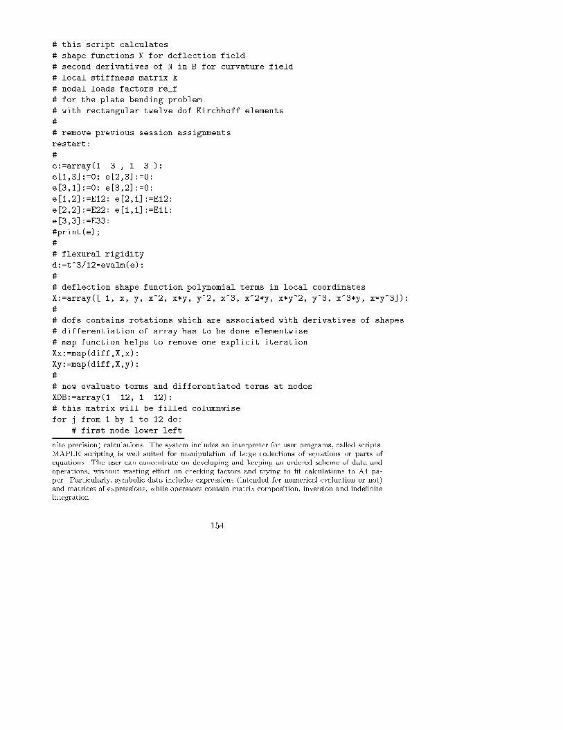
# this script calculates
# shape functions N for deflection field
# second derivatives of N in B for curvature field
# local stiffness matrix k
# nodal loads factors re_f
# for the plate bending problem
# with rectangular twelve dof Kirchhoff elements
#
# remove previous session assignments
restart:
#
e:=array(1..3 , 1..3 ):
e[1,3]:=0: e[2,3]:=0:
e[3,1]:=0: e[3,2]:=0:
e[1,2]:=E12: e[2,1]:=E12:
e[2,2]:=E22: e[1,1]:=E11:
e[3,3]:=E33:
#print(e);
#
# flexural rigidity
d:=t^3/12*evalm(e):
#
# deflection shape function polynomial terms in local coordinates
X:=array([ 1, x, y, x^2, x*y, y^2, x^3, x^2*y, x*y^2, y^3, x^3*y, x*y^3]):
#
# dofs contains rotations which are associated with derivatives of shapes
# differentiation of array has to be done elementwise
# map function helps to remove one explicit iteration
Xx:=map(diff,X,x):
Xy:=map(diff,X,y):
#
# now evaluate terms and differentiated terms at nodes
XDB:=array(1..12, 1..12):
# this matrix will be filled columnwise
for j from 1 by 1 to 12 do:
# first node lower left
nite precision) calculations. The system includes an interpreter for user programs, called scripts.MAPLE scripting is well suited for manipulation of large collections of equations or parts ofequations. The user can concentrate on developing and keeping an ordered scheme of data andoperations, without wasting e�ort on checking factors and trying to �t calculations to A4 pa-per. Particularly, symbolic data includes expressions (intended for numerical evaluation or not)and matrices of expressions, while operators contain matrix composition, inversion and inde�niteintegration.
154

XDB[1,j]:=subs(x=-a, y=-b, X[j]):
XDB[2,j]:=subs(x=-a, y=-b, Xx[j]):
XDB[3,j]:=subs(x=-a, y=-b, Xy[j]):
# second node lower right
XDB[4,j]:=subs(x=a, y=-b, X[j]):
XDB[5,j]:=subs(x=a, y=-b, Xx[j]):
XDB[6,j]:=subs(x=a, y=-b, Xy[j]):
# third node upper right
XDB[7,j]:=subs(x=a, y=b, X[j]):
XDB[8,j]:=subs(x=a, y=b, Xx[j]):
XDB[9,j]:=subs(x=a, y=b, Xy[j]):
# fourth node upper left
XDB[10,j]:=subs(x=-a, y=b, X[j]):
XDB[11,j]:=subs(x=-a, y=b, Xx[j]):
XDB[12,j]:=subs(x=-a, y=b, Xy[j]):
od:
#
# invert to get matrix of shape function coefficients
alphas:=linalg[inverse](XDB):
#
# fix the shape functions as elements of a single row
N:=linalg[innerprod]( X, alphas):
# note that evalm doesnt work here as it doesnt count a single row as
# a matrix
#
# B with double derivatives of shape fcns
# as bending uses curvature which is from twice diffs of deflection
# construct BCOM for B at element center of mass (local x,y=0,0 )
# B needed for stiff matrix and BCOM for fast eval of curvature
B:=array( 1..3, 1..12):
BCOM:=array( 1..3, 1..12):
for j from 1 by 1 to 12 do:
B[1,j]:=diff(N[j],x,x):
B[2,j]:=diff(N[j],y,y):
B[3,j]:=diff(N[j],x,y)+diff(N[j],y,x):
BCOM[1,j]:=subs(x=0,y=0,B[1,j]):
BCOM[2,j]:=subs(x=0,y=0,B[2,j]):
BCOM[3,j]:=subs(x=0,y=0,B[3,j]):
od:
#
# then set the integrand to the stiffness matrix
F:=evalm(transpose(B)&*d&*B):
#
155

# integrate
# here one can use the map function since all elements will be
# equally operated upon
k:=map(int,F,x=-a..a):
k:=map(int,k,y=-b..b):
k:=map(simplify,k):
#print(k);
#
# construct nodal loads factor
# assume transversal force surface density constant over element
re_f:=map(int,N,x=-a..a):
re_f:=map(int,re_f,y=-b..b):
re_f:=map(simplify,re_f):
#print(re_f);
#
# the below code fragment is suitable for matlab readable output
# note that if the save command would be used instead, matrix elements wont be
# stored in order
writeto(`bendstiff.sol`);
for i from 1 by 1 to 12 do:
for j from 1 by 1 to 12 do:
lprint(cat(`k(`,i,`,`,j,`)=`),k[i,j],`;`):
od:
od:
for j from 1 by 1 to 12 do:
lprint(cat( `re_f(`,j,`)=` ),re_f[j],`;`):
od:
for i from 1 by 1 to 3 do:
for j from 1 by 1 to 12 do:
lprint(cat( `BCOM(`,i,`,`,j,`)=` ),BCOM[i,j],`;`):
od:
od:
writeto(terminal);
Loading forces that are applied laterally to the sheet will give rise to bending. The
forces must be properly integrated to be used in the source column of the discretized
bending equation. If the load is q N/m2, the element source column is
re =
ZA
NT qdA (7.53)
where N is the matrix with basis functions.
156

y(mm) w; x(mm=m)
40 0 0.930 1.855 2.767 3.660 4.525
32 0 0.987 1.967 2.935 3.882 4.799
24 0 1.031 2.057 3.068 4.057 5.015
16 0 1.064 2.121 3.164 4.184 5.171
8 0 1.084 2.1608 3.222 4.261 5.265
0 0 1.090 2.173 3.242 4.286 5.297
0 8 16 24 32 40 x(mm)
y(mm) w; y(mm=m)
40 5.309 5.278 5.185 5.031 4.816 4.543
32 4.305 4.280 4.204 4.078 3.903 3.680
24 3.262 3.242 3.184 3.088 2.955 2.786
16 2.189 2.176 2.137 2.073 1.983 1.869
8 1.099 1.092 1.073 1.040 0.995 0.938
0 0 0 0 0 0 0
0 8 16 24 32 40 x(mm)
Table 7.3: Rotations when not magnetized
7.6.4 Nonmagnetized case
A simulation with only gravity as lateral force was carried out to give a reference
shape at zero ux density. This case occurs repetitively when ux density is sinu-
soidal and will give the largest de ection, as the pole pieces won't be magnetized
and only act as simple supports. Elastic sti�ness coe�cients used were E11=170.5
GPa, E22=227.3 GPa, E12=68.2 GPa and E33=74 GPa. Maximum de ection was
calculated to 0.8 mm/m on a space discretization with 225 elements for a quadrant
of the sample. The midline de ection curve can be seen in Fig. 7.5 and equilines
of de ection in Fig. 7.6.
7.6.5 Rolling direction magnetization
Active poles feeding the sample are on the x-directed yoke. Nodes on top of those
poles are set as clamped. Nodes on top of the poles of the y-yoke are set as free,
except on the inner edges where nodes are simply supported. De ection of the
y = 0 midline can be seen in Fig. 7.7. Numerical results are stated in Table 7.4,
where also curvatures and ux densities of the middle element row are printed. An
overview of the de ection �eld can be seen in Fig. 7.8. It is seen that clamping due
to reluctance force gives a low de ection gradient, which is midsurface rotation,
157

−0.15 −0.1 −0.05 0 0.05 0.1 0.15
0
0.05
0.1
0.15
0.2
x
z
Figure 7.7: Geometry in m for the cut y = 0 when x-magnetized. Deformation
of sheet magni�ed with factor 50. Flux density vectors drawn. Undeformed sheet
dash-dotted.
close to the active poles and leakage seems not to be large enough to counteract
this behaviour. Leakage reluctance force density is 16 N=m2 localized to an element
column 12 mm wide around poles. Compare to gravity force density 17.6 N=m2
over the whole surface.
7.6.6 Transversal magnetization
Simulations with y-directed yoke exciting the sheet transversely have also been
done. Boundary conditions are as in the x-excitation case, but rotated 90 degrees
in the sheet plane. De ections for the midline connecting the poles are seen in Fig.
7.7 and numerically stated in Table 7.5. Equilines of de ection can be seen in Fig.
7.8. Leakage is larger when trying to excite the anisotropic sheet transversely, but
it shows no greater e�ect as it is still quite localized around the pole pieces.
7.6.7 Experiments
Experiments with measuring sample re ector tilts have been performed. The setup
is schematically drawn in Fig. 7.11. The screen where the spot position was mea-
sured was located 3.1 m from the re ecting micro prism. The light beam deviation
change from the xy-plane with parallel incidence on prisms placed at (x; y) with
158

y(mm) w; x(mm=m)
40 0 0.848 1.682 2.485 3.242 3.932
32 0 0.898 1.781 2.632 3.433 4.164
24 0 0.938 1.860 2.748 3.584 4.347
16 0 0.967 1.916 2.832 3.693 4.478
8 0 0.984 1.951 2.882 3.758 4.557
0 0 0.990 1.962 2.899 3.780 4.584
0 8 16 24 32 40 x(mm)
y(mm) w; y(mm=m)
40 3.358 3.330 3.248 3.112 2.925 2.691
32 2.716 2.693 2.626 2.516 2.364 2.174
24 2.053 2.036 1.985 1.901 1.786 1.642
16 1.376 1.364 1.330 1.274 1.196 1.100
8 0.690 0.684 0.667 0.638 0.600 0.551
0 0 0 0 0 0 0
0 8 16 24 32 40 x(mm)
Table 7.4: Rotations when x-magnetized
−0.15 −0.1 −0.05 0 0.05 0.1 0.15−0.15
−0.1
−0.05
0
0.05
0.1
0.15
Figure 7.8: Equilines of de ection (solid) when x-magnetized. Outlines of pole
surfaces (dash-dotted).
159

−0.15 −0.1 −0.05 0 0.05 0.1 0.15
0
0.05
0.1
0.15
0.2
y
z
Figure 7.9: Geometry in m for the cut x = 0 when y-magnetized. De ection of
sheet magni�ed with factor 50. Flux density vectors drawn. Undeformed sheet
dash-dotted.
y(mm) w; x(mm=m)
40 0 0.486 0.9699 1.448 1.919 2.378
32 0 0.528 1.054 1.575 2.086 2.584
24 0 0.562 1.122 1.676 2.220 2.748
16 0 0.587 1.172 1.750 2.317 2.868
8 0 0.602 1.202 1.795 2.376 2.941
0 0 0.607 1.212 1.810 2.396 2.965
0 8 16 24 32 40 x(mm)
y(mm) w; y(mm=m)
40 4.022 3.999 3.930 3.814 3.654 3.449
32 3.329 3.310 3.252 3.157 3.024 2.856
24 2.560 2.546 2.501 2.428 2.326 2.197
16 1.737 1.727 1.697 1.647 1.578 1.490
8 0.877 0.872 0.857 0.832 0.797 0.753
0 0 0 0 0 0 0
0 8 16 24 32 40 x(mm)
Table 7.5: Rotations when y-magnetized
160

−0.15 −0.1 −0.05 0 0.05 0.1 0.15−0.15
−0.1
−0.05
0
0.05
0.1
0.15
Figure 7.10: Equilines of de ection (solid) when y-magnetized. Outlines of pole
surfaces (dash-dotted).
front surface normals -(cos �, sin �) is
'de = �2�(w;x(x; y) cos�+ w;y(x; y) sin�) (7.54)
The change can be computed from Table 7.4 or Table 7.5 subtracted with the
reference values in Table 7.3. Measured values are found in Table 7.6. They agree
very well for the TD-excited case, while the LD-excitation presents 40% lower x-
rotation change and 25% higher y-rotation change in computations. This might be
due to elastic and magnetic anisotropy data of the actual sample di�ering from the
typical data used in simulations.
~B-dir. 12j 'de j (mrad)
LD 1.1 1.6
TD 2.3 1.3
(40,0) (0,40) x; y(mm)
0 90 �(deg)
Table 7.6: Experimental results
161
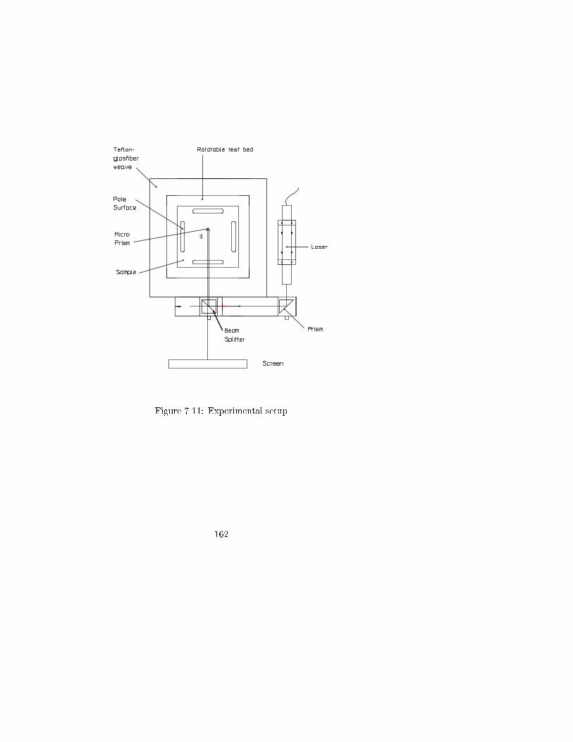
Figure 7.11: Experimental setup
162

Chapter 8
Measurement and
veri�cation
8.1 Introduction
Measurements with focus on magnetostriction are reported. Magnetization mea-
surements, uniaxial and rotating, are presented brie y at the end.
Because the conventional sheet is considerably more magnetostrictive with ~B in
the transversal direction (measured magnetocompliance 4:1 �10�11Pa�1 > 10 times
having ~B in the rolling direction) there has been a focus on measuring with this
direction of excitation.
Measurements of the transverse magnetostriction from a likewise oriented mag-
netic ux density in a conventional grain oriented silicon-iron sheet are presented.
A data processing scheme to extract nonlinearity and frequency dependency pa-
rameters from such measurements is shown. A good �t is obtained with six reals
representing ux density excitation, four for material nonlinearity and three for
time rate dependency.
The magnetostrictive strain component is �My and the ux density component is
By. The rolling and transverse directions of the sheet are here x and y respectively.The butter y curve of double-valued strain vs. ux density is made single-valued
by a least squares procedure. A �t to a nonlinear function of the magnetic stress1�0B2y is performed. The time lag of strain to magnetic stress is modelled by a
163

rate-dependent equation. The equation is solved in the frequency domain with
a magnetic stress from a �ltered ux density. At present it is unclear if rate-
dependency is dominating over hysteresis in the 50 to 250 Hz ux frequency region
considered. The model is nevertheless useful as a parameterization in simulation
programs and as a well-de�ned hypothesis to further test with experiment. Model
use in a �nite element surrounding is indicated.
8.2 Experiments
The magnetic setup has been described in [101], and it is here used to feed the
sample with an alternating ux density in the y-direction, which is known to cause
the greatest magnetostrictive response of these materials. The optical setup has
been presented in earlier chapters. The strain information is retrieved by a single
non-contact interferometer, which illuminates a pair of sample re ectors M that
senses the elongation of a 70 mm element. L is a stabilized HeNe laser, P are prisms,
AOM is an acousto-optic modulator, BS are beamsplitters, M1 is a mirror and PD
is a photodiode. The AOM facilitates intensity alteration when the interferometer is
operated in homodyne mode, and can impose a carrier on the temporal interference
pattern to operate the interferometer in heterodyne mode. The sample test bed
with feeding yokes is possible to rotate, so strain components can be measured in
turn while preserving the same excitation. In this paper results are restricted to the
transverse strain component. The ux density waveform can be seen as squared in
Fig. (8.2). The peak ux density is 0:7 T and the �rst harmonic is at 50 Hz. Two
odd harmonics are signi�cant, the third and �fth at 150 and 250 Hz respectively.
The third has a magnitude of 19 % to the �rst harmonic and the �fth 10 %. The
response �My has a peak value of 15 �m=m and is shown in Fig. 8.2. By plotting
�My versus By one gets the butter y curve, shown in Fig. 8.4. Of further interest
is the plot of �My to B2y , which can be seen as a strain-stress diagram, yielding
magnetoelastic potential energy from an averaged single-valued curve and a loss
proportional to the area of the loop.
8.3 Data processing and nonlinear model
The creation of a single-valued magnetostriction curve is done by interpolation,
averaging and least squares polynomial �tting. The butter y curve is interpolated
in equally spaced strain points, to catch the �M peak in the lossless curve rather
than the B peak. The averaged curve is then least squares �tted to a polynomial.
The last action can be shown as equal to �nding the polynomial that minimizes the
164

0 0.002 0.004 0.006 0.008 0.01 0.012 0.014 0.016 0.018 0.020
0.05
0.1
0.15
0.2
0.25
0.3
0.35
0.4
0.45
0.5
Time [s]
Flu
x de
nsity
squ
ared
[T^2
]
Figure 8.1: Measured (solid) and simulated (dash-dotted) B2(t).
distance to both ux density branches in a least squares sense. The lossless strain
curve is here expressed as a third order polynomial in powers of the magnetic stress.
By introducing the scaling values �M = �M (tp), Bs = B(tp) where tp is strain peak
time, one can write the polynomial using an orthogonal function sequence as
�MA(B2)=� = d0 + d1f1(B2=B2
s) + d2f2(B2=B2
s ) + d3f3(B2=B2
s ) (8.1)
f1 = x� 1=2 (8.2)
f2 = x2 � x+ 1=6 (8.3)
f3 = x3 � 3=2x2 + 3=5x� 1=20 (8.4)
Fitting to single-valued data gave d0 = 0.5378, d1 = 0.8485, d2 = -0.0594 and d3= 1.3266. It is seen that energy quotas E3=E1 � 1% and E2=E1 � 0:03% where
Ei = d2i kfik2 = d2iR 10fi(x)
2dx. So the need for nonlinear terms in this region is
slight.
To get a short description of the exciting ux density, a Fourier expansion is done
with following ideal �ltering out of the signi�cant harmonics. One can write the
cut o� Fourier expansion and the identi�cation of the coe�cients Bi as
Bsim(t) =
3Xi=1
(B2i�1ej(2i�1)!1t +B�
2i�1e�j(2i�1)!1t) (8.5)
165

0 0.002 0.004 0.006 0.008 0.01 0.012 0.014 0.016 0.018 0.02−2
0
2
4
6
8
10
12
14
16
Time [s]
Mag
neto
stric
tion
[mum
/m]
Figure 8.2: Measured (solid) and simulated (dash-dotted) �M (t).
−0.8 −0.6 −0.4 −0.2 0 0.2 0.4 0.6 0.80
2
4
6
8
10
12
14
16
Flux density [T]
Mag
neto
stric
tive
stra
in [m
icro
m/m
]
Figure 8.3: Measured butter y loops of �My vs. By, solid, and single-valued �tted
curve, dash-dotted.
166

−0.8 −0.6 −0.4 −0.2 0 0.2 0.4 0.6 0.8−2
0
2
4
6
8
10
12
14
16
Flux density [T]
Mag
neto
stric
tion
[mum
/m]
Figure 8.4: Magnetostriction curves, measured (solid) and simulated with nonlinear
model (dash-dotted).
Bi =
NXk=1
B(kTs)e�ji2�k=N ; Ts =
2�
N!1(8.6)
where the last expression is seen to be equal to 1=N times the fast Fourier transform.
The number of sample points N in the time trace is 256 and the �rst harmonic
angular frequency !1 is 2�50 rad/s. The squared �ltered ux density is then
B2sim(t) = C0 +
5Xi=1
(C2iej2i!1t + C�
2ie�j2i!1t) (8.7)
C2i = g(Bl) i = 0; 1:::5 l = 1; 3; 5 (8.8)
where g is given by the relations
C0 = 2jB1j2 + 2jB5j2 + 2jB3j2 (8.9)
C2 = 2B�1B3 + 2B�
3B5 +B21 (8.10)
C4 = 2B�1B3 + 2B�
1B5 (8.11)
C6 = 2B�1B5 +B2
3 (8.12)
C8 = 2B3B5 (8.13)
C10 = B25 (8.14)
167

0 0.05 0.1 0.15 0.2 0.25 0.3 0.35 0.4 0.45 0.5−2
0
2
4
6
8
10
12
14
16
Flux density squared [T^2]
Mag
neto
stric
tion
[mum
/m]
Figure 8.5: Magnetostriction curves, measured (solid) and simulated with nonlinear
model (dash-dotted).
168

It is necessary to use g since direct �ltering of B2 gives a signal with negative values
which is unphysical. Carrying on to the expression for the lossless magnetostriction,
with the knowledge of there being a third order relation to this entity, Eq. (8.1),
one can write
�MAsim (t) = F0 +
15Xi=1
(F2iej2i!1t + F �
2ie�j2i!1t) (8.15)
F2i = e(C2m; dn) i = 0; 1:::15 m = 0; 1:::5 n = 0; 1:::3 (8.16)
The relation (8.16) is analogous to the previous case of squaring of the ux density,
but this time for a third order combination of �ve harmonics and thus too lengthy
to write out here. The coe�cients Fi are determined via e � g from the ux density
coe�cients Bj and the model parameters dk. The signals simulated in this way are
seen in Fig. (8.2).
8.4 Frequency dependence
Loop �ts are carried out by a frequency domain method. It is assumed that the
magnetostriction obeys a linear di�erential equation with the lossless magnetostric-
tion as the primary driving entity. The greatest loop width comes from a lag of the
100 Hz component of �M to �MA. There is an approximate 90 degree phase shift
of the 200 Hz component in the presented measurement, so a resonant model has
to be used. The resonance can also be seen in the butter y curve as a crossing of
the branches at a nonzero ux density. The 300 Hz component has a low leading
phase, so to catch that, there has to be a zero in the transfer function ~�M=~�MA at
some complex frequency. For simplicity that frequency is chosen as real here. The
above yields
~�M (f) =�(f=fd2)2 + 1
�(f=fr2)2 + jf=fr1 + 1~�MA def
= H(f)~�MA(f) (8.17)
where ~�M (f) is the Fourier coe�cient at frequency f . The parameters for the curvesshown are fr1 = 900 Hz, fr2 = 193:5 Hz, and fd2 = 215:5 Hz.
8.5 2D model from measurements
The use of a linear model in simulation programs is now illustrated. The mag-
netostriction to be incorporated as a strain source in a �nite element scheme [93]
169

−0.8 −0.6 −0.4 −0.2 0 0.2 0.4 0.6 0.80
2
4
6
8
10
12
14
16
Flux density [T]
Mag
neto
stric
tion
[mum
/m]
Figure 8.6: Magnetostriciton curves, measured (solid) and simulated with linear
model (dash-dotted).
170

0 0.05 0.1 0.15 0.2 0.25 0.3 0.35 0.4 0.45 0.50
2
4
6
8
10
12
14
16
Flux density squared [T^2]
Mag
neto
stric
tion
[mum
/m]
Figure 8.7: Magnetostriction curves, measured (solid) and simulated with linear
model (dash-dotted).
171

is 24 ~�Mx
~�My~�Mxy
35 = H(f)
24 Di
11 Di12 0
Di21 Di
22 0
0 0 Di33
3524 ~B2
x=B2xs
~B2y=B
2ys
~BxBy=BxsBys
35 (8.18)
where Dikl are scaled magnetocompliances at frequency f = 2if1; i = 0; 1::5. Bxs
and Bys are scaling levels. The scaling levels are adjusted to the measurement
ranges which should ideally cover the region up to saturation. The factoring out of
a single transfer function H(f) is strictly not possible, but merely indicates the �rststep of a tensorial extension of the frequency dependency. The construction of the
magnetic shear stress ~BxBy is straightforward from harmonic interaction of Fourier
coe�cients Bxi and Byi. For the present single direction low peak measurements,
the linear model yields fair results as seen in Fig. (8.7).
8.6 Magnetization measurements
The setup can make nice ux density versus �eld strength measurements. This ca-
pability is shown for three examples of excitation of an oriented sheet. In Fig. 8.8,
the sample was subjected to a �eld strength uniaxially alternating in the rolling
direction. In Fig. 8.9, the sample was subjected to a �eld strength uniaxially
alternating in the transverse direction. The characteristic initial bend of the mag-
netization curve in the transverse direction is seen.
The third case was with a rotating �eld excitation applied to the specimen. The
�rst �gure Fig. 8.10 shows the ux density locus of the rotational process. One
can see that the natural locus of the material resembles a rhombus (also known as
the lozenge or diamond shape). The hardest directions are at right angles to the
side of the rhombus, 56� from the rolling direction when estimated by eye from the
graph. A slight misalignment of 1-2� of the measurement coils can also be seen.
The second �gure Fig. 8.11 shows the �eld strength locus for a cycle. The angle
to the maxima of the �eld strength is roughly 53�, also indicating the direction of
hard magnetization.
For more results on magnetization the reader is referred to the articles co-written
by the author [15] [106].
172

-2
-1.5
-1
-0.5
0
0.5
1
1.5
2
-1000 -800 -600 -400 -200 0 200 400 600 800 1000
B_r
dH
_rd
B_r
d
H_rd
Figure 8.8: Flux density [T] in rolling direction versus �eld strength [A/m] in rolling
direction. Oriented material.
-1.5
-1
-0.5
0
0.5
1
1.5
-2500 -2000 -1500 -1000 -500 0 500 1000 1500 2000 2500
H_td
B_t
d
Figure 8.9: Flux density [T] in transverse direction versus �eld strength [A/m] in
transverse direction. Oriented material.
173
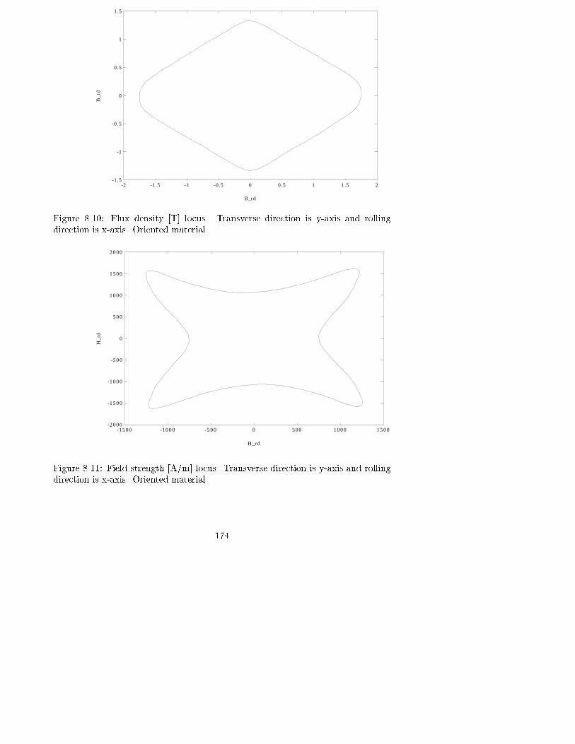
-1.5
-1
-0.5
0
0.5
1
1.5
-2 -1.5 -1 -0.5 0 0.5 1 1.5 2
B_rd
B_t
d
Figure 8.10: Flux density [T] locus. Transverse direction is y-axis and rolling
direction is x-axis. Oriented material.
-2000
-1500
-1000
-500
0
500
1000
1500
2000
-1500 -1000 -500 0 500 1000 1500
H_rd
H_t
d
Figure 8.11: Field strength [A/m] locus. Transverse direction is y-axis and rolling
direction is x-axis. Oriented material.
174

Chapter 9
Conclusions and future work
9.1 Conclusions
9.1.1 Setup uses
The described measurement setup is a good supplier of magnetostriction and mag-
netization material characteristics. Together with �nite element- friendly parametriza-
tion techniques, like the one shown in the last chapter, it can provide support for
the analysis and optimization of magnetically excited silicon-iron structures. Be-
cause of the e�ciency of the user interface, magnetization measurements can be
done quickly. It can therefore be used for routine hysteresis, loss, permeability
and saturation measurements. Magnetostriction measurements take longer time
because of the need of interferometer alignment.
Magnetization of nonoriented and conventional grain-oriented samples can easily
be measured in di�erent directions or with a rotating vector because of the double
yoke system. Superoriented samples are more di�cult to saturate in the transversal
direction if double yokes are used, and the operator might have to only use one yoke
in that situation. The measurement of magnetostriction in di�erent directions is
simpli�ed by the possibility of rotating the sample holder with the yokes.
175

9.1.2 Sample �eld calculation
Field calculations have resulted in an estimation of ux density and strain �eld
size and homogeneity in the central part of a non-oriented silicon-iron sample sheet
subjected to inhomogeneous magnetostrictively induced strain without applied ex-
ternal loads. The ux density homogeneity is fair and magnetic �eld sensors can
be made from coils that have signi�cant length. The local strain corresponds fairly
well to the local magnetostrictive strain.
A constitutive relation for rate-dependent magnetostrictive strain suitable for con-
tinuum magnetomechanical simulations of oriented silicon-iron sheets has been
proposed. The shape of the magnetostriction loop when excited by a sinusoidal
magnetic ux is fairly well represented in the rolling and transverse directions.
Computations of total strain magnitude and phase �elds are feasible. In a typical
grain-oriented material one is able to calculate the relative in uence of elasticity on
magnetostrictive strain to total strain.
9.1.3 Bending
The bending rotation of a silicon-iron sheet in a magnetic and gravitational �eld
was studied. It was found that rotation changes during the magnetization cy-
cle could give laser beam deviation changes up to 4.6 mrad when re ectors were
mounted 40 mm o� from the sheet center. This beam vibration can have serious
e�ects on recombination in an interferometer for displacement or magnetostriction
measurements if not considered and componentwise properly compensated for. Use
the sample holder table, and �ll out the air gaps from the yoke to the sample to
make the surface under the sample plane. Use fairly light loads such as steel bars
to atten any nonplanar imperfection of the sample. Check with measurement of
the spot vibration of a beam re ected by a prism mounted at on the triangular
side.
9.1.4 Magnetostriction harmonics
In the single sheet tester that is more current than voltage controlled, the ux den-
sity waveform will be distorted due to saturation e�ects. When the ux density
contains three frequencies, the magnetic stress and the single-valued magnetostric-
tion can be well represented with harmonic interaction formulas from nonlinearity.
The lagging magnetostriction is gotten by a transfer function operating on the
single-valued magnetostriction.
176
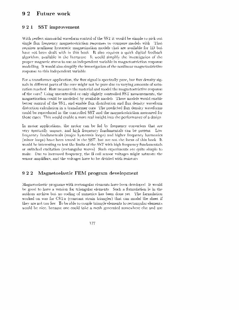
9.2 Future work
9.2.1 SST improvement
With perfect sinusoidal waveform control of the SST it would be simple to pick out
single ux frequency magnetostriction responses to compare models with. That
requires nonlinear hysteretic magnetization models that are available for 1D but
have not been dealt with in this book. It also requires a quick digital feedback
algorithm, available in the literature. It would simplify the investigation of the
proper magnetic stress to use as independent variable in magnetostriction response
modelling. It would also simplify the investigation of the nonlinear magnetostrictive
response to this independent variable.
For a transformer application, the ux signal is spectrally pure, but ux density sig-
nals in di�erent parts of the core might not be pure due to varying amounts of satu-
ration reached. How measure the material and model the magnetostrictive response
of the core? Using uncontrolled or only slightly controlled SST measurements, the
magnetization could be modelled by available models. These models would enable
better control of the SST, and enable ux distribution and ux density waveform
distortion calculation in a transformer core. The predicted ux density waveforms
could be reproduced in the controlled SST and the magnetostriction measured for
those cases. This would enable a more real insight into the performance of a design.
In motor applications, the motor can be fed by frequency converters that are
very spectrally unpure, and high frequency fundamentals can be present. Low
frequency fundamentals (major hysteresis loops) and higher frequency harmonics
(minor loops) have been tested in the SST, but are not the focus of this book. It
would be interesting to test the limits of the SST with high frequency fundamentals
or switched excitation (rectangular waves). Such experiments are quite simple to
make. Due to increased frequency, the B-coil sensor voltages might saturate the
sensor ampli�ers, and the voltages have to be divided with resistors.
9.2.2 Magnetoelastic FEM program development
Magnetoelastic programs with rectangular elements have been developed. It would
be good to have a version for triangular elements. Such a formulation is in the
authors archive but no coding of numerics has been done yet. The formulation
worked on was for CST:s (constant strain triangles) that can model the sheet if
they are not too few. To be able to couple triangle elements to rectangular elements
would be nice, because one could take a mesh generated somewhere else and use
177
it for magnetoelastic calculations with the same element numbering. Making an
extension to 3D would be interesting because one could try to model stacks of
sheets with 3D elements, where each element corresponds to a large number of
sheets within its thickness. This would allow the study the magnetoelastic e�ects
of clamping devices applied normally to the sheet, for example. The ux could
be allowed to be unevenly distributed over the normal direction to the stack. The
weakening introduced by the lamination compared to a solid block would have to
be considered. The shear moduli in the zx and zy planes, where z is normal to
stack, would be lowered.
9.2.3 Magnetostriction measurements
More magnetostriction measurements need to be done. Complete three axis strain
measurements should be done for di�erent directions of magnetic excitation. Higher
ux densities should be tested. The onset of frequency dependency should be
determined with di�erent frequency tests. The use of the acousto-optic modulator
to determine the sign of strain should be put into practice.
178

179

Chapter 10
List of symbols
Symbol styles
a scalar
~a vector
ai Cartesian component of vector$a tensor
aij Cartesian component of tensor
C matrix
d column (single column matrix)
dxy column for x-y coordinate system
�u column
ui column entry
�un iteration numbered column
s(m) element numbered matrix or column
Cij matrix entry
Cxy matrix used in x-y coordinate system
CT transposed matrix
CC complex conjugate
C�1 inverted matrix
C�1ij component of inverted matrix
? convolution operator
~g Fourier decomposed function
I peak value of function
S indetermined form of S matrix
@x partial derivative w.r.t. x-coordinate (@i w.r.t. i:th coord.)
@xy second partial derivative w.r.t. x and y coordinates
@ domain boundary
180

Uppercase Latin symbols~A (magnetic) vector potential
A area
A transformation matrix~B (magnetic) ux density
B shape function derivative matrix
C (elastic) compliance matrix
D magnetocompliance matrix
D bending sti�ness (can be a matrix)
E elasticity matrix
Eij elasticity coe�cient~F force
F Fourier decomposition
G shear modulus (isotropic case)
Gi shear modulus (orthotropic case)
I (electric) current~J (electric) current density
K global sti�ness matrix
K dispersion kernel
L inductance~M magnetization
M bending moment per unit length
Ni shape (or basis) function
O major ordo
P magnetoelastic modulus (uniaxial stress)
Q magnetoelastic shear modulus (isotropic case)
Qi magnetoelastic shear modulus (orthotropic case)
R resistance
R reluctance
S global magnetic sti�ness matrix
S indeterminate global magnetic sti�ness matrix
T temperature
T� transformation matrix for stress column
T� transformation matrix for strain column
U column of unknowns
U voltage, electromotive force
V (electric scalar) potential
V (magnetic) scalar potential
X reactance
Y Young's modulus (uniaxial stress elastic modulus)
Z impedance
181

Lowercase Latin symbols
aij direction cosine between i:th primed coordinate direction and j:th unprimed dir.
a half of rectangular element length
a table side length
b half of rectangular element width
bi derivative of approximation of H2=2 w.r.t. nodal value uic table thickness
c speed of light or of sound
cL longitudinal wave speed
cP pressure wave speed
cS shear wave speed
cB bending wave speed�f excitation column~f body force, force per volume unit
f frequency
fc carrier frequency
fm modulating frequency
i input variable
i index (integer)
j index
j imaginary unit
k index
k local sti�ness matrix
l index
m index
n number of nodes
nx number of nodes in x direction
ny number of nodes in y dirnz number of nodes in z dirq load, force/area
q (equivalent) magnetic charge
~r position vector
�r residual column
s local magnetic sti�ness matrix
s shape function gradient scalar product matrix
t element thickness~t traction vector
�u column of nodal values
u exact or approximate solution
u output variable
u energy density
182

u(i) displacement at node i
ui displacement at node i
~u displacement vector
u displacement in x direction
v displacement in y directionw displacement in z directionw weight function
x horizontal coordinate
y vertical coordinate
z lateral coordinate
Uppercase Greek symbols
� boundary
� di�erence, increase
�x coordinate di�erence
�x linearized change operator for x direction (= �x@x)� product
� sum
� ux
linked ux
domain
Lowercase Greek symbols
� thermal expansion coe�cient
�i thermal expansion coe�cient in i:th direction
� angle of material direction change
� angle of material direction change
�i direction cosine, relative to i:th direction
xy shear angle (= 2�xy)� di�erence, increase
�ij Kronecker delta, (�ij = 1 if i = j, else 0)$� (total) strain tensor$�M magnetostrictive strain tensor
�ij strain tensor component
�x normal strain in x-direction (= �xx)�y normal strain in y-direction (= �yy)�xy shear strain (= xy=2)� engineering strain column = [�x; �y; xy]
T
$�M magnetostrictive strain
� angle from speci�ed direction or plane
� angle from z-direction� curvature
183

� magnetostriction
�s magnetostriction of magnetically saturated material
� wavelength
� �rst Lame constant
� second Lame constant
� permeability
�i permeability in i:th direction
�0 vacuum permeability
�r relative permeability
� Poisson ratio (lateral contraction ratio at isotropy)
�i directional cosines
~� direction, unity vector
� magnetoelastic lateral contraction ratio
� acos(-1)
� mass density
� charge density
�m magnetic pole density
�s surface charge density
� (electric) conductivity$� stress tensor$�M magnetic stress tensor
�ij stress tensor component
� stress column =[�x; �y ; �xy]T
� normal stress
� shear stress
�ij shear stress component, i 6= j' polar angle
� (magnetic) scalar potential
� diameter
� (magnetic) susceptibility
! angular frequency
184

Chapter 11
List of units
A ampere
A/m ampere per meter
A=m2 ampere per square meter
H henry
mH millihenry
H�1 per henry
H/m henry per meter
Hz hertz
kHz kilohertz
J joule
J=m3 joule per cubic meter
N newton
N/m newton per meter
N=m2 newton per square meter
Nm newtonmeter
ohm
Pa pascal
S siemens
T tesla
V volt
V/m volt per meter
W watt
W/kg watt per kilogram
W=m2 watt per square meter
185

Wb weber
mWb milliweber
�Wb microweber
Wb/m weber per meter
deg degree
g gram
kg kilogram
m meter
mm millimeter
�m micrometer
nm nanometer
m2 square meter
m3 cubic meter
m�1 per meter
m=m meter per meter
�m=m micrometer per meter
m/s meter per second
m=s2 meter per second per second
mrad milliradian
rad radian
rad/s radian per second
s second
186

Bibliography
[1] D. Jiles and D. Ahterton, \Theory of ferromagnetic hysteresis," Journal of
Magnetism and Magnetic Materials, no. 61, pp. 48{60, 1986.
[2] D. C. Jiles, J. B. Thoelke, and M. K. Devine, \Numerical determination
of hysteresis parameters for the modeling of magnetic properties using the
theory of ferromagnetic hysteresis," IEEE Transactions on Magnetics, vol. 28,
pp. 27{35, Jan. 1992.
[3] D. C. Jiles, \Frequency dependence of hysteresis curves in ferromagnetic ma-
terials," in IEEE Transactions on Magnetics, INTERMAG, 1993.
[4] A. Adly, I. Mayergoyz, and A. Bergqvist, \Preisach modeling of magnetostric-
tive hysteresis," J. Appl. Phys., vol. 69, p. 5777, 1991.
[5] A. Bergqvist and G. Engdahl, \A stress-dependent magnetic Preisach hys-
teresis model," IEEE Trans. Mag., vol. 27, p. 4796, 1991.
[6] L. Kvarnsj�o, A. Bergqvist, and G. Engdahl, \Application of a stress-
dependent magnetic Preisach hysteresis model on a simulation model for
Terfenol-D," IEEE Trans. Mag., vol. 28, p. 2623, 1992.
[7] A. Bergqvist and G. Engdahl, \A phenomenological di�erential{relation{
based vector hysteresis model," J. Appl. Phys., vol. 75, p. 5484, 1994.
[8] A. Bergqvist and G. Engdahl, \A phenomenological magnetomechanical hys-
teresis model," J. Appl. Phys., vol. 75, p. 5896, 1994.
[9] A. Bergqvist, On magnetic hysteresis modeling. PhD thesis, KTH, 1994.
[10] A. Bergqvist and G. Engdahl, \A model for magnetomechanical hysteresis
and losses in magnetostrictive materials," J. Appl. Phys., vol. 79, p. 6476,
1996.
187
[11] G. Engdahl, F. Stillesj�o, and A. Bergqvist, \Performance simulations of mag-
netostrictive actuators with resonant mechanical loads." presented at ACTU-
ATOR 96, Bremen, Germany.
[12] A. Bergqvist and G. Engdahl, \A thermodynamic representation of pseu-
doparticles with hysteresis," IEEE Trans. Mag., vol. 31, p. 3539, 1995.
[13] A. J. Bergqvist, \A thermodynamic vector hysteresis model for ferromagnetic
materials," in Nonlinear electromagnetic systems (A. J. Moses and A. Basak,
eds.), p. 528, Amsterdam: IOS Press, 1996.
[14] A. Bergqvist, \Magnetic vector hysteresis model with dry friction{like pin-
ning," Physica B., vol. 233, p. 342, 1997.
[15] A. Bergqvist, A. Lundgren, and G. Engdahl, \Experimental testing of an
anisotropic vector hysteresis model," IEEE Trans. Mag., vol. 233, p. 4152,
1997.
[16] P. Holmberg, A. Bergqvist, and G. Engdahl, \Modelling eddy currents and
hysteresis in a transformer laminate," IEEE Trans. Mag., March 1997. in
press.
[17] C. Bengtsson, \Dom�anstrukturer i sife pl�at," Postgraduate course UPTEC
82131 R, ISSN 0346-8887, Institute of Technology, Uppsala University, Avd.
for fasta tillstandets fysik, Inst. for teknologi, Uppsala Universitet, Box 534,
751 21 Uppsala, 1982. Bengtsson is now (1994) manager of ABB Transformers
development laboratory in Ludvika, Sweden.
[18] E. W. Lee, \The [110] magnetostriction of some single crystals of iron and
silicon-iron," Proc. Phys. Soc., vol. LXVIII, no. 2A, pp. 65{71, 1954.
[19] M. Celasco and P. Mazetti, \Magnetostriction of grain-oriented ferromagnetic
cubic materials," J. Phys. D: Appl. Phys., vol. 5, pp. 1604{1613, 1972.
[20] P. Allia, A. Ferro-Milone, G. Montalenti, G. P. Soardo, and F. Vinai, \Theory
of negative magnetostriction in grain oriented 3and applied stresses," IEEE
Transactions on Magnetics, vol. MAG-14, pp. 362{364, Sept. 1978.
[21] P. Allia, M. Celasco, A. Ferro, A. Masoero, and A. Stepanescu, \Transverse
closure domains and the behavior of the magnetization in grain-oriented poly-
crystalline magnetic sheets," J. Appl. Phys., vol. 52, pp. 1439{1447, Mar.
1981.
[22] G. Bertotti, P. Mazetti, and G. P. . Soardo, \A general model of losses in soft
magnetic materials," Journal of Magnetism and Magnetic Materials, no. 26,
pp. 225{233, 1982.
188

[23] J. Bishop, \Asymmetric domain wall bowing and tilting motins in materials
with orientations between (100)[001] and (110)[001]," Journal of Magnetism
and Magnetic Materials, no. 26, pp. 247{251, 1982.
[24] J. E. L. Bishop, \Simulation of skew domain wall bowing in sife lamina-
tions with asymmetric roll orientation," IEEE Transactions on Magnetics,
vol. MAG-18, no. 4, pp. 970{981, 1982.
[25] T. Yamaguchi, \E�ect of sheet thickness on magnetostriction characteristics
of 3 percent si-fe single crystals with slightly inclined (110)[001] orientation,"
IEEE Transactions on Magnetics, vol. MAG-20, pp. 2033{2036, Sept. 1984.
[26] M. Imamura, T. Sasaki, and T. Yamaguchi, \Domain-wall eddy-current loss
in a stripe domain structure of si-fe crystals inclined slightly from the per-
fect (110)[001] orientation," IEEE Transactions on Magnetics, vol. MAG-20,
pp. 2120{2129, Nov. 1984.
[27] A. J. Moses, \Measurement of magetostriction and vibration with regard to
transformer noise," IEEE Transactions on Magnetics, vol. MAG-10, pp. 154{
156, June 1974.
[28] A. J. Moses, \Magnetostriction measurements at high stress levels in si-fe and
co-fe alloys," Journal of Magnetism and Magnetic Materials, no. 26, pp. 185{
186, 1982.
[29] D. J. Mapps and C. E. White, \Longitudinal and transverse magnetostric-
tion harmonics in (110)[001] silicon-iron," IEEE Transactions on Magnetics,
vol. MAG-20, pp. 1566{1568, Sept. 1984.
[30] A. J. Moses and C. P. Bakopolous, \E�ect of stress annealing on loss and
magnetostriction in grain-oriented silicon-iron," manuscript copy.
[31] P. Allia, A. Ferro, G. P. Soardo, and F. Vinai, \Magnetostriction behavior in
isotropic and cube-on-face 3vol. 50, no. 11, pp. 7716{7718, 1979.
[32] H. Pf�utzner, \Domain interactions between stacked hi-b sife sheets," IEEE
Transactions on Magnetics, vol. MAG-18, pp. 961{962, July 1982.
[33] K. Fukawa and T. Yamamoto, \Domain structures and stress distributions
due to ball-point scratching in 3(110)[001]," IEEE Transactions on Magnetics,
vol. MAG-18, pp. 963{969, July 1982.
[34] H. Pf�utzner, C. Bengtsson, and A. Leeb, \Domain investigation on coated
unpolished si-fe sheets," IEEE Transactions on Magnetics, vol. MAG-21,
pp. 2620{2625, Nov. 1985.
189

[35] G. C. Eadie, \The e�ects of stress and temperature on the magnetostriction
of commercial 3.25Journal of Magnetism and Magnetic Materials, no. 26,
pp. 43{46, 1982.
[36] H. J. Stanbury, \Magnetostriction e�ects at angles to the rolling direction
in grain-oriented 3.25% silicon-steel," Journal of Magnetism and Magnetic
Materials, no. 26, pp. 47{49, 1982.
[37] B. Hribernik, \In uence of cutting strains on the magnetic anisotropy of
fully processed silicon steel," Journal of Magnetism and Magnetic Materials,
no. 26, pp. 72{74, 1982.
[38] J. Slama and M. Prejsa, \Investigation of magnetization mechanisms in ori-
ented si-fe sheets," Journal of Magnetism and Magnetic Materials, no. 26,
pp. 239{242, 1982.
[39] J. V. S. Morgan and K. J. Overshott, \An experimental veri�cation of the
ruckling process in electrical sheet steel," Journal of Magnetism and Magnetic
Materials, no. 26, pp. 243{246, 1982.
[40] V. Ungemach, \Dependence of the domain structure of sife single crystals on
the frequency of demagnetizing �elds," Journal of Magnetism and Magnetic
Materials, no. 26, pp. 252{254, 1982.
[41] V. M. Bichard, \The observation of domain structures in grain oriented si-fe
using a high voltage scanning electron microscope," Journal of Magnetism
and Magnetic Materials, no. 26, pp. 255{257, 1982.
[42] S. A. Zhou and R. K. T. Hsieh, \A theoretical model of eddy current nonde-
structive test for electromagnetoelastic materials," Int. J. Engng Sci., vol. 26,
no. 1, pp. 12{26, 1988.
[43] T. Nozawa, M. Mizogami, H. Mogi, and Y. Matsuo, \Domain structures
and magnetic properties of advanced grain-oriented silicon steel," Journal of
Magnetism and Magnetic Materials, vol. 133, pp. 115{122, 1994.
[44] H. Masui, M. Mizokami, Y. Matsuo, and H. Mogi, \A proposal of predicting
formulae for in uence of stress on magnetostriction in grain oriented silicon
steel," ISIJ International, vol. 35, no. 4, pp. 409{418, 1995.
[45] S. Arai and A. Hubert, \The pro�les of lancet-shaped surface domains in
iron," Phys. stat. sol. (a), vol. 147, pp. 563{568, 1995.
[46] Y. Nakamura, Y. Okazaki, J. Harase, and N. Takahashi, \The dc and ac
magnetic properties of a high-purity grain-oriented iron sheet," Journal of
Magnetism and Magnetic Materials, vol. 133, pp. 153{155, 1994.
190

[47] H. Masui, \In uence of stress condition on initiation of magnetostriction in
grain oriented silicon steel," IEEE Transactions on Magnetics, vol. 31, no. 2,
pp. 930{937, 1995.
[48] R. Vasina, \Changes of ferromagnetic parameters during cyclic stressing,"
phys stat sol (a), no. 137, pp. 189{196, 1993.
[49] C. S. Schneider, P. Y. Cannell, and K. T. Watts, \Magnetoelasticity for large
stresses," IEEE Transactions on Magnetics, vol. 28, pp. 2626{2631, Sept.
1992.
[50] H. Maeda, K. Harada, Y. Ishihara, and T. Todaka, \Performance of mag-
netostriction of silicon steel sheet with bias �eld," in Proc. of the 12th Soft
Magnetic Materials Conference, 1995. PB-26.
[51] T. E. Carlsson and N. Abramson, \Short-coherence-length multipass inter-
ferometer," Optics letters, vol. 20, no. 10, pp. 1187{1188, 1995.
[52] H. Mogi, M. Yabumoto, M. Mizokami, and Y. Okazaki, \Harmonic analysis of
ac magnetostriction measurements under non-sinusoidal excitation," in Proc.
of the Intermag'96 Conference, 1996.
[53] T. Lewis, J. Llewellyn, and M. van der Sluijs, \Electrokinetic properties of
metal-dielectric interfaces," IEE Proceedings-A, vol. 140, no. 5, pp. 385{392,
1993.
[54] T. Nakata, N. Takahashi, M. Nakano, K. Muramatsu, and M. Miyake, \Mag-
netostriction measurements with a laser doppler velocimeter," Joint INTER-
MAG MMM, 1994. Paper No. AQ-04.
[55] T. Nakata, N. Takahashi, K. Fujiwara, and M. Nakano, \Measurements of
magnetic characteristics along arbitrary directions of grain-oriented silicon
steel up to high ux densities," IEEE Transactions on Magnetics, vol. 29,
pp. 3544{3546, November 1993.
[56] Y. Ohtsuka and M. Tsubokawa, \Dynamic two-frequency interferometry for
small displacement measurements," Optics and Laser Technology, pp. 25{29,
February 1984.
[57] Y. Ohtsuka and K. Itoh, \Two-frequency laser interferometer for small dis-
placement measurements in a low frequency range," Applied Optics, vol. 18,
pp. 219{224, January 1979.
[58] C. R. G. Higgs and A. J. Moses, \Computation of ux distribution and har-
monics in various transformer cores," Journal of Magnetism and Magnetic
Materials, no. 26, pp. 349{350, 1982.
191

[59] T. Nakata, N. Takahashi, and Y. Kawase, \Finite element analysis of magnetic
�elds taking into account hysteresis characteristics," IEEE Transactions on
Magnetics, vol. MAG-21, pp. 1856{1858, Sept. 1985.
[60] T. Nakata and N. Takahashi, \Application of the �nite element method to the
design of permanent magnets," IEEE transactions on Magnetics, vol. MAG-
18, no. 6, pp. 1049{1051, 1982.
[61] T. Nakata, \Numerical analysis of ux and loss distributions in electrical
machinery," IEEE Transactions on Magnetics, vol. MAG-20, pp. 1750{1755,
Sept. 1984. Invited paper.
[62] T. Nakata, N. Takahashi, Y. Kawase, H. Funakoshi, and S. Ito, \Finite ele-
ment analysis of magnetic circuits composed of axisymmetric and rectangu-
lar regions," IEEE Transactions on Magnetics, vol. MAG-21, pp. 2199{2202,
Nov. 1985.
[63] T. Nakata, N. takahashi, and Y. Kawase, \New approximate method for cal-
culating three-dimensional magnetic �elds in laminated cores," IEEE Trans-
actions on Magnetics, vol. MAG-21, pp. 2374{2377, Nov. 1985.
[64] \Approximation analysis of three-dimensional magnetic �elds in iron cores
laminated with grain-oriented silicon steel," Electrical Engineering in Japan,
vol. 1987, no. 6, pp. 90{97, 1987.
[65] D. Pavlik, D. C. Johnson, and R. S. Girgis, \Calculation and reduction of
stray and eddy losses in core-form transformers using a highly accurate �nite
element modelling technique," in IEEE/PES 92 Winter Meeting, IEEE Power
Engineering Society, 1992. Auhors 1 & 2 are with Westinghouse, 3 is with
ABB T&D Indiana.
[66] T. Doong and I. D. Mayergoyz, \On numerical implementation of hysteresis
models," IEEE Transactions on Magnetics, vol. MAG-21, pp. 1853{1855,
Sept.
[67] A. Bergqvist and G. Engdahl, \A phenomenological di�erential-relation-based
vector hysteresis model," J. Appl. Phys., vol. 75, no. 10, pp. 5484{5486, 1994.
[68] A. Bergqvist and G. Engdahl, \A phenomenological magnetomechanical hys-
teresis model," J. Appl. Phys., vol. 75, no. 10, pp. 5496{5498, 1994.
[69] T. P�era, F. Ossart, and T. Waeckerle, \Field computation in non linear
anisotropic sheets using the coenergy model," IEEE Transactions on Mag-
netics, Sept. 1993.
[70] T. P�era, F. Ossart, and T. Waeckerle, \Numerical representation for
anisotropic materials based on coenergy modelling," J. Appl. Phys., vol. 73,
pp. 6784{6786, May 1993.
192

[71] P. P. Silvester and D. Omeragi�c, \Di�erentiation algorithms for soft magnetic
material models," in IEEE Transactions on Magnetics, INTERMAG, 1993.
Paper no. EQ-05.
[72] M. Gyimesi and J. Lavers, \Generalized potential formulation for 3{D magne-
tostatic problems," IEEE Transactions on Magnetics, vol. MAG-28, pp. 1924{
1929, July 1992.
[73] M. Kaltenbacher, H. Landes, and R. Lerch, \An e�cient calculation scheme
for the numerical simulation of coupled magnetomechanical systems," in Proc.
of CEFC'96, March 1996.
[74] M. Kaltenbacher, H. Landes, and R. Lerch, \Simulation tool for magnetome-
chanical systems with moving parts," in Proc. of the ISEM Conf., 1995.
[75] Y. Yoshida, K. Demachi, and K. Miya, \Scaling law for magnetoelastically
coupled vibration of thin conducting components in a fusion reactor," in Proc.
of the ISEM Conf., 1995.
[76] K. Matsubara, N. Takahashi, K. Fujiwara, and T. Nakata, \Acceleration
technique of waveform control for single sheet tester," in Proc. of the Intermag
Conf., 1995.
[77] T. Nakata and N. Takahashi, \Analysis of ux distributions in three-phase
�ve-legged recti�er transformer cores," Electrical Engineering in Japan,
vol. 100, no. 6, pp. 42{50, 1980.
[78] T. Nakata, N. Takahashi, and Y. Kawase, \Flux and loss distribution in
the overlap joints of laminated cores," Journal of Magnetism and Magnetic
Materials, no. 26, pp. 343{344, 1982.
[79] T. Nakata and Y. Kawase, \Analysis of the magnetic characteristics in the
straight overlap joint of laminated cores," 1982.
[80] T. Nakata, Y. Ishihara, N. Takahashi, and Y. Kawase, \Analysis of magnetic
�elds in a single sheet tester using an h coil.," Journal of Magnetism and
Magnetic Materials, no. 26, pp. 179{180, 1982.
[81] T. Nakata, N. Takahashi, Y. Kawase, and M. Nakano, \In uence of lami-
nation orientation and stacking on magnetic characteristics of grain-oriented
silicon steel laminations," IEEE Transactions on Magnetics, pp. 1774{1776,
Sept. 1984.
[82] T. Erlandsson and L. Martinsson, \Investigation of no-load losses and distri-
bution of magnetic ux in transformer cores with step-lap joints," Examen-
sarbete 1993 03 04, ABB Transformers, 1993.
193
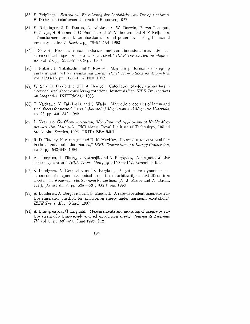
[83] E. Reiplinger, Beitrag zur Berechnung der Lautst�arke von Transformatoren.
PhD thesis, Technischen Universit�at Hannover, 1972.
[84] E. Reiplinger, J. P. Fanton, A. Adobes, A. W. Darwin, P. van Leemput,
F. Claeys, H. H�uttner, J. G. Paulick, A. J. M. Verhoeven, and H. F. Reijnders,
\Transformer noise: Determination of sound power level using the sound
intensity method," �Electra, pp. 79{95, Oct. 1992.
[85] J. Sievert, \Recent advances in the one- and two-dimensional magnetic mea-
surement technique for electrical sheet steel," IEEE Transaction on Magnet-
ics, vol. 26, pp. 2553{2558, Sept. 1990.
[86] T. Nakata, N. Takahashi, and Y. Kawase, \Magnetic performance of step-lap
joints in distribution transformer cores," IEEE Transactions on Magnetics,
vol. MAG-18, pp. 1055{1057, Nov. 1982.
[87] W. Salz, M. Birkfeld, and K. A. Hempel, \Calculation of eddy current loss in
electrical steel sheet considering rotational hysteresis," in IEEE Transactions
on Magnetics, INTERMAG, 1993.
[88] T. Yagisawa, Y. Takekoshi, and S. Wada, \Magnetic properties of laminated
steel sheets for normal uxes," Journal of Magnetism and Magnetic Materials,
no. 26, pp. 340{342, 1982.
[89] L. Kvarnsj�o, On Characterization, Modelling and Application of Highly Mag-
netostrictive Materials. PhD thesis, Royal Institute of Technology, 100 44
Stockholm, Sweden, 1993. TRITA-EEA-9301.
[90] R. D. Findlay, N. Stranges, and D. K. MacKay, \Losses due to rotational ux
in three phase induction motors," IEEE Transactions on Energy Conversion,
no. 3, pp. 543{548, 1994.
[91] A. Lundgren, H. Tiberg, L. Kvarnsj�o, and A. Bergqvist, \A magnetostrictive
electric generator," IEEE Trans. Mag., pp. 3150 { 3152, November 1993.
[92] S. Lundgren, A. Bergqvist, and S. Engdahl, \A system for dynamic mea-
surements of magnetomechanical properties of arbitrarily excited silicon-iron
sheets," in Nonlinear electromagnetic systems (A. J. Moses and A. Basak,
eds.), (Amsterdam), pp. 528 { 531, IOS Press, 1996.
[93] A. Lundgren, A. Bergqvist, and G. Engdahl, \A rate-dependent magnetostric-
tive simulation method for silicon-iron sheets under harmonic excitation,"
IEEE Trans. Mag., March 1997.
[94] A. Lundgren and G. Engdahl, \Measurements and modeling of magnetostric-
tive strain of a transversely excited silicon iron sheet," Journal de Physique
IV, vol. 8, pp. 587{590, June 1998. Pr2.
194

[95] A. Lundgren, A. Bergqvist, and G. Engdahl, \Analysis and veri�cation of
anisotropic magnetic sheet bending in an inhomogeneous lateral �eld," in
XI Conference on the Computation of Electromagnetic Fields (J. Cardoso,
J. Bastos, and N. Ida, eds.), (Belo Horizonte, Brazil), pp. 287 { 288, Sociedade
Brasileira de Eletromagnetismo, November 1997.
[96] T. Nakata, N. Takahashi, and M. Nakano, \Improvments of measuring equip-
ments for rotational power loss," in 1st International Workshop on Magnetic
Properties of electrical sheet steel under two{dimensional excitation, (Braun-
schweig), Physikalisch{Technische Budesanstalt, 1992.
[97] D. K. Cheng, Field and wave electromagnetics. Addison-Wesley, 2 ed., 1990.
[98] K. Binns, P. Lawrenson, and C. Trowbridge, The analytical and numerical
solution of electric and magnetic �elds. Wiley, 1992.
[99] R. Becker, Electromagnetic �elds and interactions. Dover, 1982. Originally
published by Blaisdell, 1964.
[100] J. C. Maxwell, A Treatise on Electricity and Magnetism, vol. 2. Oxford
University Press, 3 ed., 1998. First published by Clarendon Press, 1891.
[101] A. Lundgren, A. Bergqvist, and G. Engdahl, \A system for dynamic mea-
surements of magnetomechanical properties of arbitrarily excited silicon-iron
sheets," in Nonlinear electromagnetic systems (A. J. Moses and A. Basak,
eds.), (Amsterdam), pp. 528 { 531, IOS Press, 1996.
[102] H. Pf�utzner and A. Hasenzagl, \Fundamental aspects of rotational magne-
tostriction," in Nonlinear electromagnetic systems (A. J. Moses and A. Basak,
eds.), (Amsterdam), pp. 374{379, IOS Press, 1996.
[103] C. Johnson, Numerical solution of partial di�erential equations by the �nite
element method. Lund, Sweden: Studentlitteratur, 1987.
[104] R. D. Cook, D. S. Malkus, and M. E. Plesha, Concepts and applications of
�nite element analysis. New York: John Wiley & Sons, 1989.
[105] A. Schulze, \Magnetostriction i.," Z. Physik, vol. 50, p. 448, 1928.
[106] A. Bergqvist, A. Lundgren, and G. Engdahl, \Computationally e�cient vec-
tor hysteresis model with ux density as known variable," in Proceedings of
the ISEM 97 conf., 1998.
195

Appendix A
Design drawings
Dimensions are in mm.
196
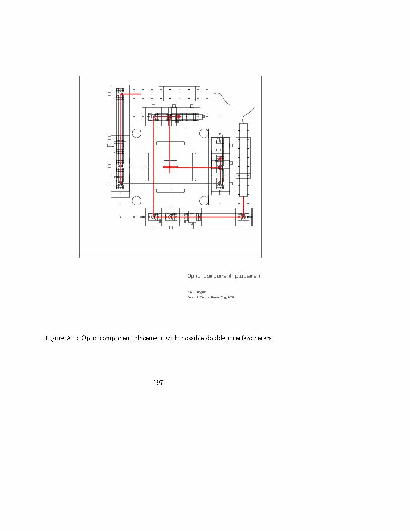
Figure A.1: Optic component placement with possible double interferometers
197

Figure A.2: Closeup of single interferometer with sample side dimension
198

Figure A.3: Side view of interferometer (possibly dual), arm with AOM
Figure A.4: Side view of interferometer (possibly dual), arm with laser head
199

Figure A.5: Laser mount
200

Figure A.6: Custom tapped rod, for optic rail on diabase spacer fastening
Figure A.7: Acoustooptic modulator, fastening on translation stage
201

Figure A.8: Baseplate for AOM
202
Figure A.9: Diabase spacers
203

Figure A.10: Sample support
204

Figure A.11: Tall laminated yoke
Figure A.12: Short laminated yoke
205

Figure A.13: Spacer between yokes
Figure A.14: Yoke pair assembly
206

Figure A.15: Table top with tapped mount holes
207

Figure A.16: Experiment table
208

Figure A.17: Table top support
209
Top Related