


Languages
Pages
Legal

On a Monte-CarloSemi-Lagrangian
scheme:variance estimateand simulations
Charles-EdouardBréhier
Description of themethod
Convergenceresults
Numerical results
Idea of the proof
Conclusion
On a Monte-Carlo Semi-Lagrangian scheme:variance estimate and simulations
Charles-Edouard Bréhier(Joint work with Erwan Faou)
ENS Cachan, Antenne de Bretagne - IRMARCERMICS, Ecole des Ponts Paris Tech & Inria
CEMRACS 2013

On a Monte-CarloSemi-Lagrangian
scheme:variance estimateand simulations
Charles-EdouardBréhier
Description of themethodThe Monte-CarlomethodTheSemi-Lagrangianscheme
Convergenceresults
Numerical results
Idea of the proof
Conclusion
The Monte-Carlo method
Problem: approximation of the solution of PDEs like
∂u(t, x)
∂t=
12
∆u(t, x) + c(x).∇u(t, x), 0 < t ≤ T , x ∈ Rd ,
u(0, x) = u0(x), for any x ∈ Rd .
Probabilistic representation:
u(t, x) = Eu0(X xt )
dX xt = c(X x
t )dt + dBt , X x0 = x .
Monte-Carlo method:
E∣∣∣ 1N
N∑m=1
u0(X x,(m)t )− u(t, x)
∣∣∣2 ≤ C(t, x)
N.
Problems:I Realizations of X x
t ? Need of a numerical scheme.I Computations at points in a grid: u(nδt, jδx). Dependence of
C(t, x) with respect to δt and δx?

On a Monte-CarloSemi-Lagrangian
scheme:variance estimateand simulations
Charles-EdouardBréhier
Description of themethodThe Monte-CarlomethodTheSemi-Lagrangianscheme
Convergenceresults
Numerical results
Idea of the proof
Conclusion
Semi-lagrangian scheme
Recursive construction of unj approximating u(nδt, jδx).
1. Representation formula between nδt and (n + 1)δt:
u((n + 1)δt, jδx) = Eu(nδt,X jδxδt );
2. Numerical scheme:
Eu(nδt, jδx + δtc(jδx) +√δtN );
3. Use of an interpolation operator J :
vn+1j := E
(J (un)(jδx + δtc(jδx) +
√δtN )
);
4. Monte-Carlo approximation:
un+1j :=
1N
N∑m=1
(J (un)(jδx + δtc(jδx) +
√δtN n,m,j )
).

On a Monte-CarloSemi-Lagrangian
scheme:variance estimateand simulations
Charles-EdouardBréhier
Description of themethodThe Monte-CarlomethodTheSemi-Lagrangianscheme
Convergenceresults
Numerical results
Idea of the proof
Conclusion
Structure of the noise
Independence of the N n,m,j ∼ N (0, I ), with respect to:
I m: Monte-Carlo approximation.Consequence: variance of size C(δt, δx)/N;
I n: independent increments/Markov property;
I j : spatial independence.
Consequences:
Improved estimate for the l2-norm:
‖u‖2l2 := δx∑
j
u2j ;
but irregular functions in the h1 semi-norm:
|u|2h1 := δx∑
j
(uj+1 − uj )2
δx2 .

On a Monte-CarloSemi-Lagrangian
scheme:variance estimateand simulations
Charles-EdouardBréhier
Description of themethod
ConvergenceresultsSimplified settingConvergenceresults
Numerical results
Idea of the proof
Conclusion
Simplified setting for a convergence estimate
In dimension d = 1.
No drift: c(x) = 0.
Boundary conditions: periodic.
Interpolation: linear.
Initial condition: u0 is of class C2.

On a Monte-CarloSemi-Lagrangian
scheme:variance estimateand simulations
Charles-EdouardBréhier
Description of themethod
ConvergenceresultsSimplified settingConvergenceresults
Numerical results
Idea of the proof
Conclusion
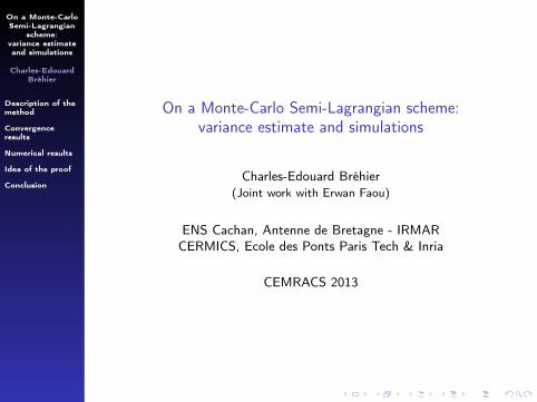
First convergence result
TheoremFor any final time T > 0, there exists a constant C > 0, such that for anyδt > 0, δx > 0 and N ∈ N∗ we have
supj∈N;0≤jδx<1
|u(nδt, xj )− vnj | ≤ C
δx2
δtsup
x∈[0,1]|u
′′0 (x)|
and for any n ∈ N with nδt ≤ T
E‖un − vn‖2l2 = δx∑
j ;0≤jδx<1
E|unj − vn
j |2
On a Monte-CarloSemi-Lagrangian
scheme:variance estimateand simulations
Charles-EdouardBréhier
Description of themethod
ConvergenceresultsSimplified settingConvergenceresults
Numerical results
Idea of the proof
Conclusion
First convergence result
TheoremFor any final time T > 0, there exists a constant C > 0, such that for anyδt > 0, δx > 0 and N ∈ N∗ we have
supj∈N;0≤jδx<1
|u(nδt, xj )− vnj | ≤ C
δx2
δtsup
x∈[0,1]|u
′′0 (x)|
and for any n ∈ N with nδt ≤ T
E‖un − vn‖2`2 ≤ 2C |u0|2h1(1 +δx2
δt)δtN
whenever N is sufficiently large:
CNA(δt, δx) ≤ 1
2.
with A(δt, δx) = 1 + δxδt + δx2
δt2 (1 + | log(δt)|).

On a Monte-CarloSemi-Lagrangian
scheme:variance estimateand simulations
Charles-EdouardBréhier
Description of themethod
ConvergenceresultsSimplified settingConvergenceresults
Numerical results
Idea of the proof
Conclusion
Second convergence result
TheoremFor any p ∈ N and any final time T > 0, there exists a constant Cp > 0, suchthat for any δt > 0, δx > 0 and N ∈ N∗ we have
supj∈N;0≤jδx<1
|u(nδt, xj )− vnj | ≤ C
δx2
δtsup
x∈[0,1]|u
′′0 (x)|
and for any n ∈ N with nδt ≤ T
E‖un − vn‖2l2 = δx∑
j ;0≤jδx<1
E|unj − vn
j |2
RemarkExplicit method, with no CFL.

On a Monte-CarloSemi-Lagrangian
scheme:variance estimateand simulations
Charles-EdouardBréhier
Description of themethod
ConvergenceresultsSimplified settingConvergenceresults
Numerical results
Idea of the proof
Conclusion
Second convergence result
TheoremFor any p ∈ N and any final time T > 0, there exists a constant Cp > 0, suchthat for any δt > 0, δx > 0 and N ∈ N∗ we have
supj∈N;0≤jδx<1
|u(nδt, xj )− vnj | ≤ C
δx2
δtsup
x∈[0,1]|u
′′0 (x)|
and for any n ∈ N with nδt ≤ T
E‖un − vn‖2l2 ≤ Cp|u0|2h1(1 +δx2
δt)A(δt, δx)p
(δtN
+1
Np+1
)with A(δt, δx) = 1 + δx
δt + δx2δt2 (1 + | log(δt)|).
RemarkExplicit method, with no CFL.

On a Monte-CarloSemi-Lagrangian
scheme:variance estimateand simulations
Charles-EdouardBréhier
Description of themethod
ConvergenceresultsSimplified settingConvergenceresults
Numerical results
Idea of the proof
Conclusion
Second convergence result
TheoremFor any p ∈ N and any final time T > 0, there exists a constant Cp > 0, suchthat for any δt > 0, δx > 0 and N ∈ N∗ we have
supj∈N;0≤jδx<1
|u(nδt, xj )− vnj | ≤ C
δx2
δtsup
x∈[0,1]|u
′′0 (x)|
and for any n ∈ N with nδt ≤ T
E‖un − vn‖2l2 ≤ Cp|u0|2h1(1 +δx2
δt)A(δt, δx)p
(δtN
+1
Np+1
).
Interpretation: anti-CFL condition and variance of size δtN .
RemarkExplicit method, with no CFL.

On a Monte-CarloSemi-Lagrangian
scheme:variance estimateand simulations
Charles-EdouardBréhier
Description of themethod
Convergenceresults
Numerical resultsIllustration of theconvergenceestimateExtensionsDirichlet boundaryconditionsA non-linearexample:2D-Burgersequations
Idea of the proof
Conclusion
Numerical illustration
Periodic case:
1.6 1.8 2 2.2 2.4 2.6 2.8 3 3.2 3.4−2.5
−2
−1.5
−1
−0.5
0
log10
(n)
log
10(E
rro
r)
N=10
N=20
N=40
N=80
theoretical
Figure: Error for periodic boundary conditions when δt = δx = 1/n, inlogarithmic scales.

On a Monte-CarloSemi-Lagrangian
scheme:variance estimateand simulations
Charles-EdouardBréhier
Description of themethod
Convergenceresults
Numerical resultsIllustration of theconvergenceestimateExtensionsDirichlet boundaryconditionsA non-linearexample:2D-Burgersequations
Idea of the proof
Conclusion
Dirichlet case:
1.6 1.8 2 2.2 2.4 2.6 2.8 3−2.8
−2.6
−2.4
−2.2
−2
−1.8
−1.6
−1.4
log10
(n)
log
10(E
rro
r)
N=10
N=20
N=40
N=80
theoretical
Figure: Error for Dirichlet boundary conditions when δt = δx = 1/n, inlogarithmic scales.

On a Monte-CarloSemi-Lagrangian
scheme:variance estimateand simulations
Charles-EdouardBréhier
Description of themethod
Convergenceresults
Numerical resultsIllustration of theconvergenceestimateExtensionsDirichlet boundaryconditionsA non-linearexample:2D-Burgersequations
Idea of the proof
Conclusion
Possible extensions
In higher dimension d ≥ 2: no change in principle for theimplementation; but for the analysis?
Addition of a drift c(x): discretization of a SDE via the Euler scheme.Analysis: need to change the norm?
Dirichlet (resp. Neumann) boundary conditions: killed (resp. reflected)diffusion processes.
Non-linear equations: more involved schemes.

On a Monte-CarloSemi-Lagrangian
scheme:variance estimateand simulations
Charles-EdouardBréhier
Description of themethod
Convergenceresults
Numerical resultsIllustration of theconvergenceestimateExtensionsDirichlet boundaryconditionsA non-linearexample:2D-Burgersequations
Idea of the proof
Conclusion
Dirichlet boundary conditions
Still in the simplified setting (d = 1, c(x) = 0).
Equation:
∂tu =12∂2
xxu;
u(t, b) = u(t, a) = 0 for any t ≥ 0,
u(0, x) = u0(x) for any x ∈ [a, b].
The probabilistic representation formula:
u(t, x) = E[u0(X xt )1t<τx ],
withτ x = inf {s > 0; x + Bs /∈ (a, b)} .
On a Monte-CarloSemi-Lagrangian
scheme:variance estimateand simulations
Charles-EdouardBréhier
Description of themethod
Convergenceresults
Numerical resultsIllustration of theconvergenceestimateExtensionsDirichlet boundaryconditionsA non-linearexample:2D-Burgersequations
Idea of the proof
Conclusion
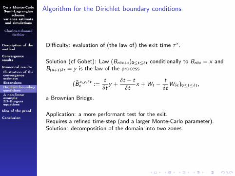
Algorithm for the Dirichlet boundary conditions
Difficulty: evaluation of (the law of) the exit time τ x .
Solution (cf Gobet): Law (Bnδt+t)0≤t≤δt conditionally to Bnδt = x andB(n+1)δt = y is the law of the process
(B̃x,y,δtt :=
tδt
y +δt − tδt
x + Wt −tδt
Wδt)0≤t≤δt ,
a Brownian Bridge.
Application: a more performant test for the exit.Requires a refined time-step (and a larger Monte-Carlo parameter).Solution: decomposition of the domain into two zones.

On a Monte-CarloSemi-Lagrangian
scheme:variance estimateand simulations
Charles-EdouardBréhier
Description of themethod
Convergenceresults
Numerical resultsIllustration of theconvergenceestimateExtensionsDirichlet boundaryconditionsA non-linearexample:2D-Burgersequations
Idea of the proof
Conclusion
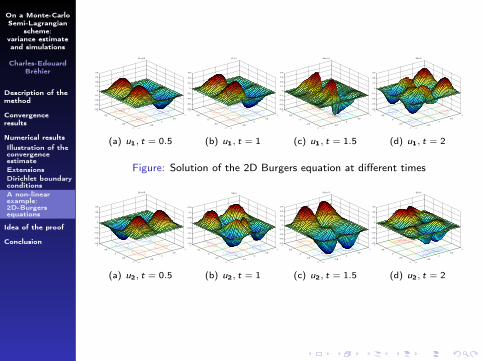
An non-linear example: 2D-Burgers equations
∂u∂t
+ (u.∇)u = ν∆u + f .
Domain (−1, 1)2, with homogeneous Dirichlet B.C.
A semi-implicit scheme: for nδt ≤ t ≤ (n + 1)δt and x ∈ D
∂vn+1
∂t+ (un.∇)vn+1 = ν∆vn+1 + f n,
with initial condition is vn+1(nδt, .) = un = vn(nδt, .).
Approximation un = vn(nδt, .).
Forcing: f n(t, x) = f (nδt, x , un(x)).

On a Monte-CarloSemi-Lagrangian
scheme:variance estimateand simulations
Charles-EdouardBréhier
Description of themethod
Convergenceresults
Numerical resultsIllustration of theconvergenceestimateExtensionsDirichlet boundaryconditionsA non-linearexample:2D-Burgersequations
Idea of the proof
Conclusion
On [nδt, (n + 1)δt]:
vn+1(t, x) = E[vn+1(nδt,X xt )1t<τx +
∫ t∧τx
nδtf n(X x
s )ds],
with
dX xt = −un(X x
t )dt +√2νdBt ,X x
nδt = x .
and the associated stopping time τ x .
Simulations: u0(x) = 0,f (t, x) = (− sin(πt) sin(πx) sin(πy)2,− sin(πt) sin(πx)2 sin(πy)),ν = 0.001.δt = 0.02, δx = 0.04, N = 10.
On a Monte-CarloSemi-Lagrangian
scheme:variance estimateand simulations
Charles-EdouardBréhier
Description of themethod
Convergenceresults
Numerical resultsIllustration of theconvergenceestimateExtensionsDirichlet boundaryconditionsA non-linearexample:2D-Burgersequations
Idea of the proof
Conclusion
−1
−0.5
0
0.5
1
−1
−0.5
0
0.5
1
−0.4
−0.3
−0.2
−0.1
0
0.1
0.2
0.3
0.4
U1,t=0.5
(a) u1, t = 0.5
−1
−0.5
0
0.5
1
−1
−0.5
0
0.5
1
−0.8
−0.6
−0.4
−0.2
0
0.2
0.4
0.6
U1,t=1
(b) u1, t = 1
−1
−0.5
0
0.5
1
−1
−0.5
0
0.5
1
−0.4
−0.3
−0.2
−0.1
0
0.1
0.2
0.3
0.4
U2,t=1.5
(c) u1, t = 1.5
−1
−0.5
0
0.5
1
−1
−0.5
0
0.5
1
−0.4
−0.3
−0.2
−0.1
0
0.1
0.2
0.3
U2,t=2
(d) u1, t = 2
Figure: Solution of the 2D Burgers equation at different times
−1
−0.5
0
0.5
1
−1
−0.5
0
0.5
1
−0.4
−0.3
−0.2
−0.1
0
0.1
0.2
0.3
U2,t=0.5
(a) u2, t = 0.5
−1
−0.5
0
0.5
1
−1
−0.5
0
0.5
1
−0.2
−0.15
−0.1
−0.05
0
0.05
0.1
0.15
U2,t=1
(b) u2, t = 1
−1
−0.5
0
0.5
1
−1
−0.5
0
0.5
1
−0.4
−0.3
−0.2
−0.1
0
0.1
0.2
0.3
0.4
U2,t=1.5
(c) u2, t = 1.5
−1
−0.5
0
0.5
1
−1
−0.5
0
0.5
1
−0.4
−0.3
−0.2
−0.1
0
0.1
0.2
0.3
U2,t=2
(d) u2, t = 2
On a Monte-CarloSemi-Lagrangian
scheme:variance estimateand simulations
Charles-EdouardBréhier
Description of themethod
Convergenceresults
Numerical results
Idea of the proof
Conclusion
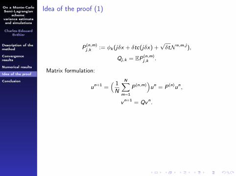
Idea of the proof (1)
P(n,m)j,k := φk(jδx + δtc(jδx) +
√δtN n,m,j ),
Qj,k = EP(n,m)j,k .
Matrix formulation:
un+1 =( 1
N
N∑m=1
P(n,m))un = P(n)un,
vn+1 = Qvn.
PropertyP(n,m) is a stochastic matrix, with independent rows.Q is symmetric.E‖P(n,m)u‖2l2 ≤ ‖u‖
2. But E|P(n,m)u|2h1?

On a Monte-CarloSemi-Lagrangian
scheme:variance estimateand simulations
Charles-EdouardBréhier
Description of themethod
Convergenceresults
Numerical results
Idea of the proof
Conclusion
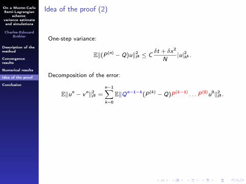
Idea of the proof (2)
One-step variance:
E‖(P(n) − Q)u‖2l2 ≤ Cδt + δx2
N|u|2h1 .
Decomposition of the error:
On a Monte-CarloSemi-Lagrangian
scheme:variance estimateand simulations
Charles-EdouardBréhier
Description of themethod
Convergenceresults
Numerical results
Idea of the proof
Conclusion
Idea of the proof (2)
One-step variance:
E‖(P(n) − Q)u‖2l2 ≤ Cδt + δx2
N|u|2h1 .
Decomposition of the error:
E‖un − vn‖2l2 =n−1∑k=0
E‖Qn−1−k(P(k) − Q)P(k−1) . . .P(0)u0‖2l2 .

On a Monte-CarloSemi-Lagrangian
scheme:variance estimateand simulations
Charles-EdouardBréhier
Description of themethod
Convergenceresults
Numerical results
Idea of the proof
Conclusion
Idea of the proof (2)
One-step variance:
E‖(P(n) − Q)u‖2l2 ≤ Cδt + δx2
N|u|2h1 .
Decomposition of the error:
E‖un − vn‖2l2 =n−1∑k=0
(Q2(n−1−k)
)1,1
E‖(P(k) − Q)P(k−1) . . .P(0)u0‖2l2 .

On a Monte-CarloSemi-Lagrangian
scheme:variance estimateand simulations
Charles-EdouardBréhier
Description of themethod
Convergenceresults
Numerical results
Idea of the proof
Conclusion
Idea of the proof (2)
One-step variance:
E‖(P(n) − Q)u‖2l2 ≤ Cδt + δx2
N|u|2h1 .
Decomposition of the error:
E‖un−vn‖2l2 =n−1∑k=0
(Q2(n−1−k)
)1,1
E‖(P(k) − Q)Qku0‖2l2
+n−1∑k=0
(Q2(n−1−k)
)1,1
E‖(P(k) − Q)(P(k−1) . . .P(0) − Qk
)u0‖2l2 .
Blue part: improved bound.Red part: recursion, with p.
On a Monte-CarloSemi-Lagrangian
scheme:variance estimateand simulations
Charles-EdouardBréhier
Description of themethod
Convergenceresults
Numerical results
Idea of the proof
Conclusion
Conclusion
I A numerical scheme combining Semi-Lagrangian and Monte-Carlotechniques.
I Simple and can be widely generalized (dimension, domains,boundary conditions).
I Example of applications: fluids, kinetic equations.
I The variance estimate: interesting but only for a simple case...I A lot to be done!
On a Monte-CarloSemi-Lagrangian
scheme:variance estimateand simulations
Charles-EdouardBréhier
Description of themethod
Convergenceresults
Numerical results
Idea of the proof
Conclusion
Conclusion
I A numerical scheme combining Semi-Lagrangian and Monte-Carlotechniques.
I Simple and can be widely generalized (dimension, domains,boundary conditions).
I Example of applications: fluids, kinetic equations.I The variance estimate: interesting but only for a simple case...
I A lot to be done!

On a Monte-CarloSemi-Lagrangian
scheme:variance estimateand simulations
Charles-EdouardBréhier
Description of themethod
Convergenceresults
Numerical results
Idea of the proof
Conclusion
Conclusion
I A numerical scheme combining Semi-Lagrangian and Monte-Carlotechniques.
I Simple and can be widely generalized (dimension, domains,boundary conditions).
I Example of applications: fluids, kinetic equations.I The variance estimate: interesting but only for a simple case...I A lot to be done!

On a Monte-CarloSemi-Lagrangian
scheme:variance estimateand simulations
Charles-EdouardBréhier
Description of themethod
Convergenceresults
Numerical results
Idea of the proof
Conclusion
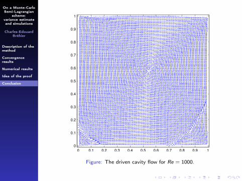
An additional example
Incompressible Navier-Stokes equations:
∂u∂t
+ (u.∇)u − ν∆u +∇p = f
div(u) = 0,
u(0, .) = u0,
+boundary conditions.
Use of a projection method:
∂vn+1
∂t+ (un.∇)vn+1 − ν∆vn+1 = f (nδt, .), (1)
and un+1 = vn+1 −∇pn+1 with
∆pn+1 = div(vn+1). (2)
Example: driven cavity, with different Reynolds numbers.
On a Monte-CarloSemi-Lagrangian
scheme:variance estimateand simulations
Charles-EdouardBréhier
Description of themethod
Convergenceresults
Numerical results
Idea of the proof
Conclusion
0 0.1 0.2 0.3 0.4 0.5 0.6 0.7 0.8 0.9 1
0
0.1
0.2
0.3
0.4
0.5
0.6
0.7
0.8
0.9
1
Figure: The driven cavity flow for Re = 1000.

On a Monte-CarloSemi-Lagrangian
scheme:variance estimateand simulations
Charles-EdouardBréhier
Description of themethod
Convergenceresults
Numerical results
Idea of the proof
Conclusion
0 0.1 0.2 0.3 0.4 0.5 0.6 0.7 0.8 0.9 1
0
0.1
0.2
0.3
0.4
0.5
0.6
0.7
0.8
0.9
1
Figure: The driven cavity flow for Re = 5000.

On a Monte-CarloSemi-Lagrangian
scheme:variance estimateand simulations
Charles-EdouardBréhier
Description of themethod
Convergenceresults
Numerical results
Idea of the proof
Conclusion
0 0.1 0.2 0.3 0.4 0.5 0.6 0.7 0.8 0.9 1
0
0.1
0.2
0.3
0.4
0.5
0.6
0.7
0.8
0.9
1
Figure: The driven cavity flow for Re = 10000.

On a Monte-CarloSemi-Lagrangian
scheme:variance estimateand simulations
Charles-EdouardBréhier
Description of themethod
Convergenceresults
Numerical results
Idea of the proof
Conclusion
Thanks for your attention.
Top Related