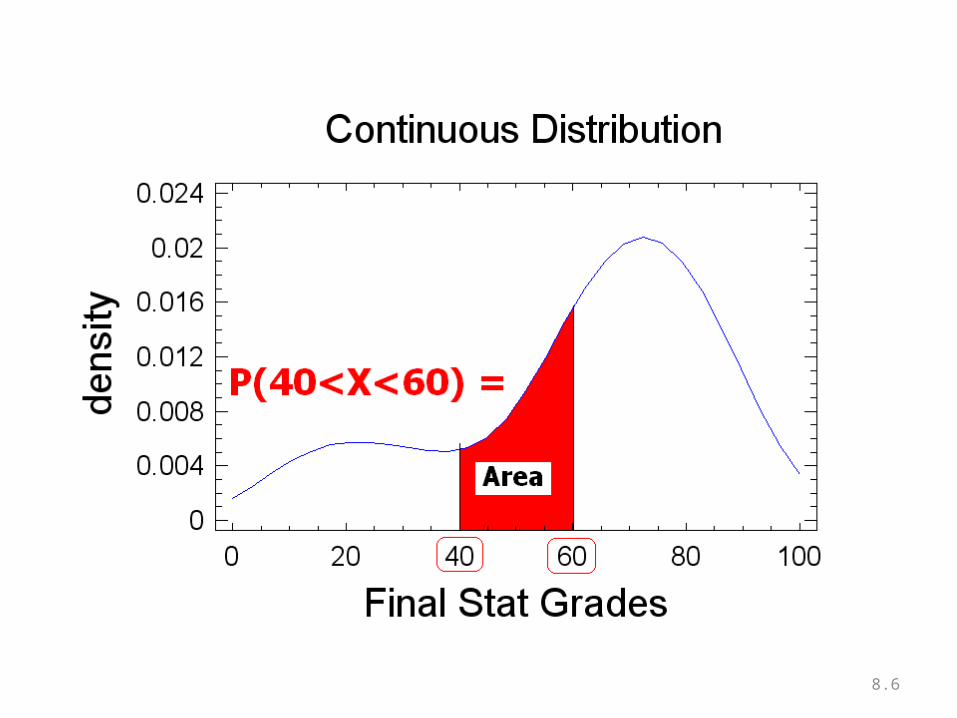
Normal Distribution

Introduction

Probability Density Functions

8.3

Probability Density Functions…

• Unlike a discrete random variable which we studied in Chapter 7, a continuous random variable is one that can assume an uncountable number of values.

• We cannot list the possible values because there is an infinite number of them.

• Because there is an infinite number of values, the probability of each individual value is virtually 0.

8.4

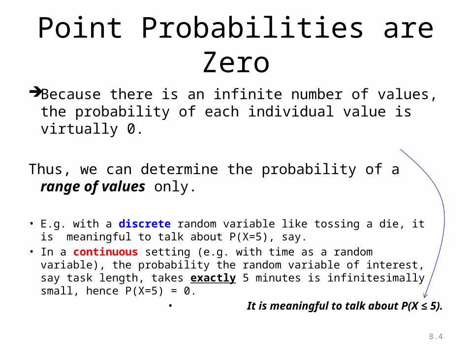
Point Probabilities are Zero

Because there is an infinite number of values, the probability of each individual value is virtually 0.

Thus, we can determine the probability of a range of values only.

• E.g. with a discrete random variable like tossing a die, it is meaningful to talk about P(X=5), say.

• In a continuous setting (e.g. with time as a random variable), the probability the random variable of interest, say task length, takes exactly 5 minutes is infinitesimally small, hence P(X=5) = 0.

• It is meaningful to talk about P(X ≤ 5).

8.5

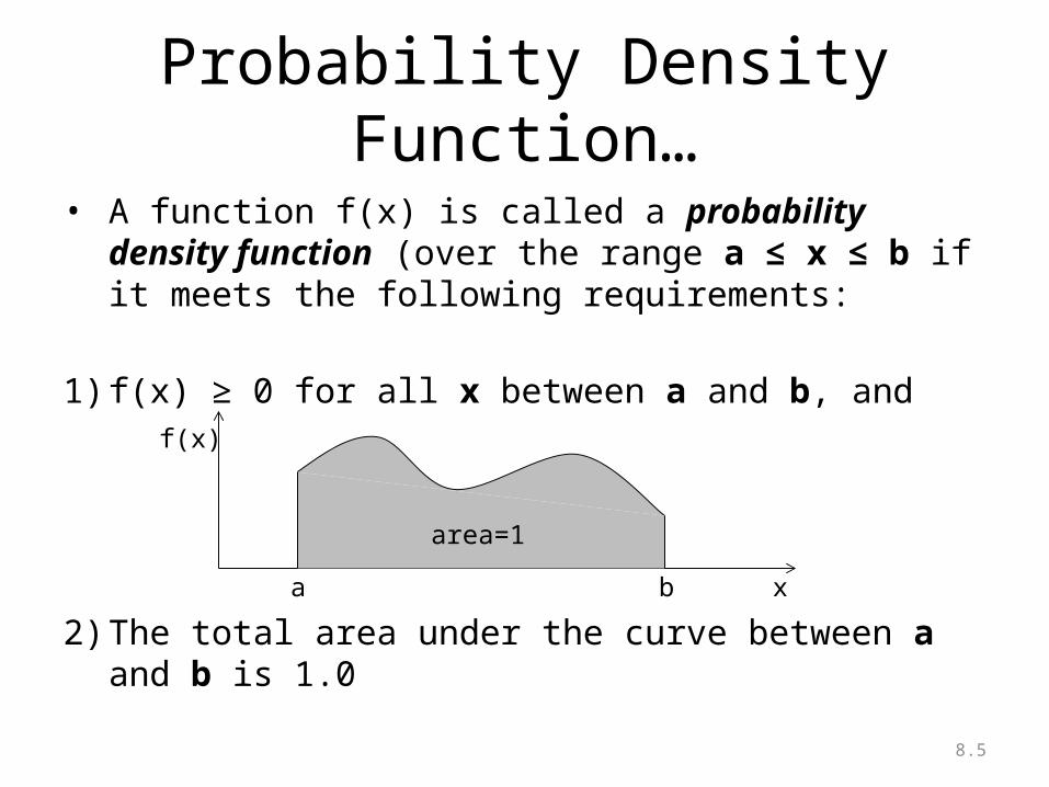
Probability Density Function…

• A function f(x) is called a probability density function (over the range a ≤ x ≤ b if it meets the following requirements:

1) f(x) ≥ 0 for all x between a and b, and

2) The total area under the curve between a and b is 1.0

f(x)

xba

area=1

8.6

8.7

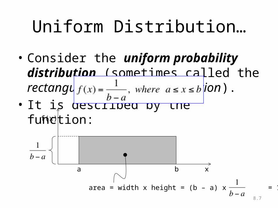
Uniform Distribution…

• Consider the uniform probability distribution (sometimes called the rectangular probability distribution).

• It is described by the function:f(x)

xba

area = width x height = (b – a) x = 1

8.8

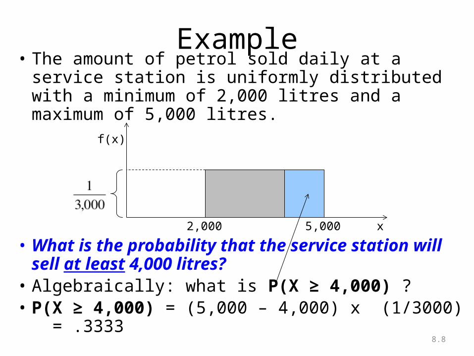
Example• The amount of petrol sold daily at a service station

is uniformly distributed with a minimum of 2,000 litres and a maximum of 5,000 litres.

• What is the probability that the service station will sell at least 4,000 litres?

• Algebraically: what is P(X ≥ 4,000) ?• P(X ≥ 4,000) = (5,000 – 4,000) x (1/3000) = .3333

f(x)

x5,0002,000

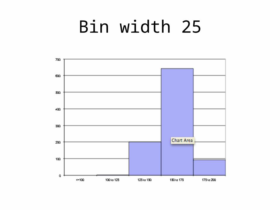
Bin width 25

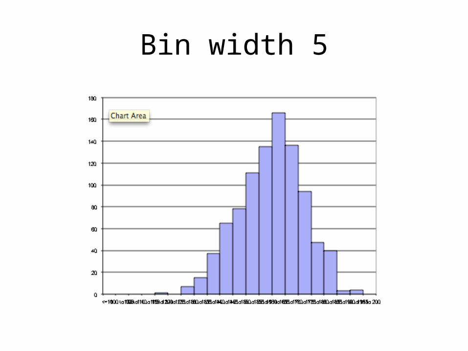
Bin width 5

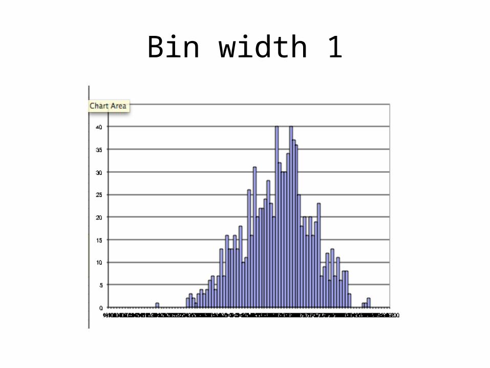
Bin width 1

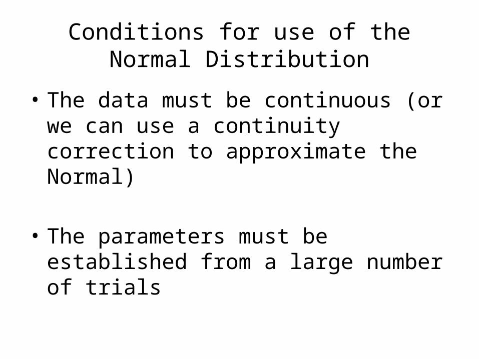
Conditions for use of the Normal Distribution

• The data must be continuous (or we can use a continuity correction to approximate the Normal)

• The parameters must be established from a large number of trials

8.14

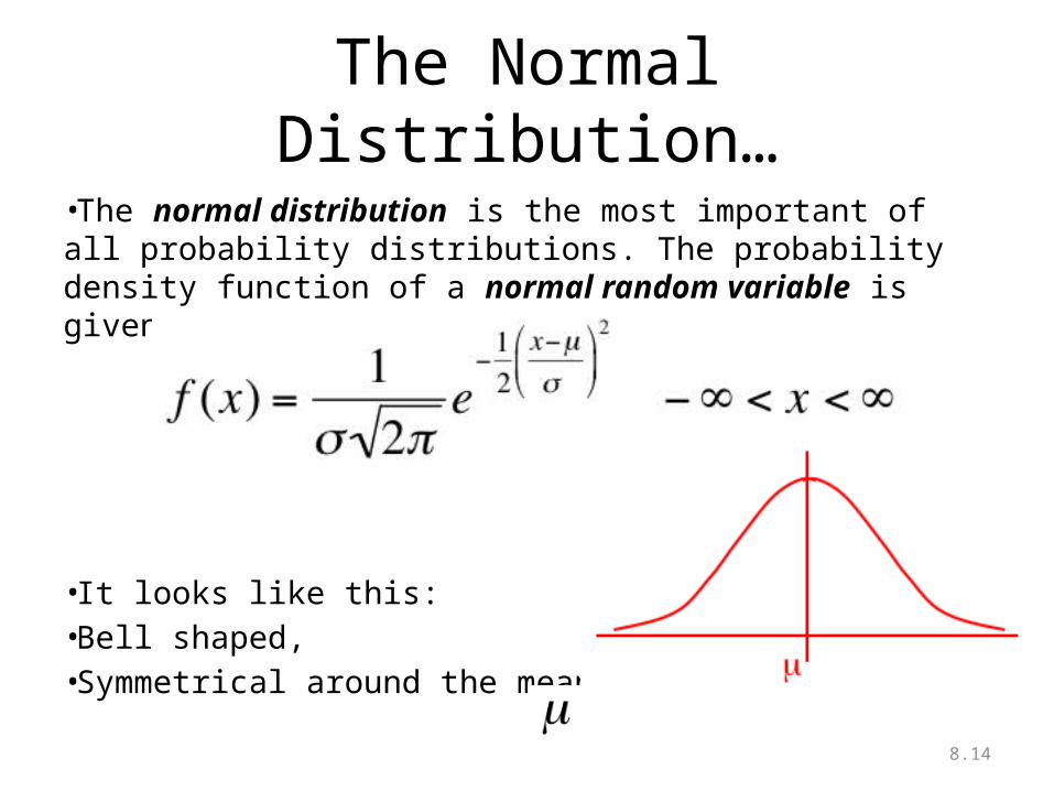
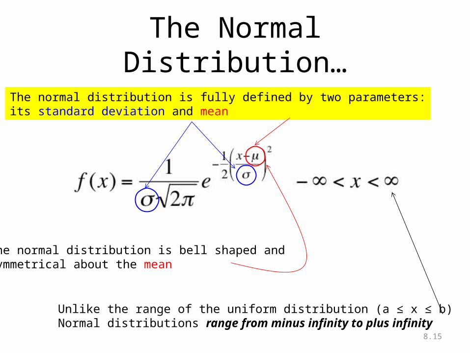
The Normal Distribution…

•The normal distribution is the most important of all probability distributions. The probability density function of a normal random variable is given by:

•It looks like this:•Bell shaped,•Symmetrical around the mean …

8.15

The Normal Distribution…

•Important things to note:The normal distribution is fully defined by two parameters:its standard deviation and mean

Unlike the range of the uniform distribution (a ≤ x ≤ b)Normal distributions range from minus infinity to plus infinity

The normal distribution is bell shaped andsymmetrical about the mean

8.16

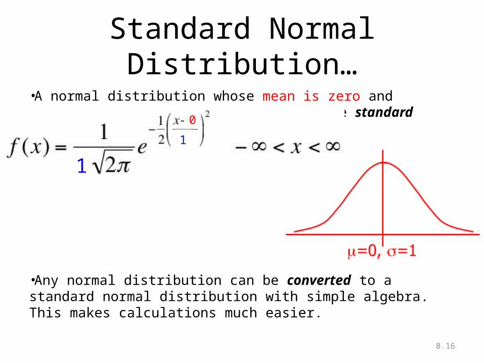
Standard Normal Distribution…•A normal distribution whose mean is zero and standard deviation is one is called the standard normal distribution.

•Any normal distribution can be converted to a standard normal distribution with simple algebra. This makes calculations much easier.

0

1

1

8.17

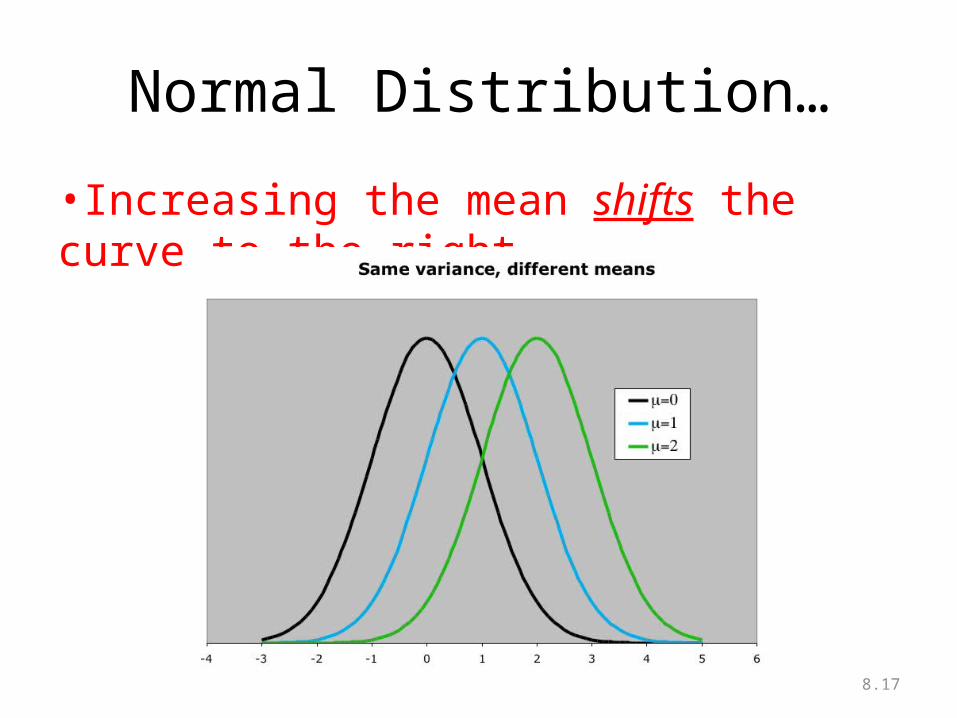
Normal Distribution…

•Increasing the mean shifts the curve to the right…

8.18

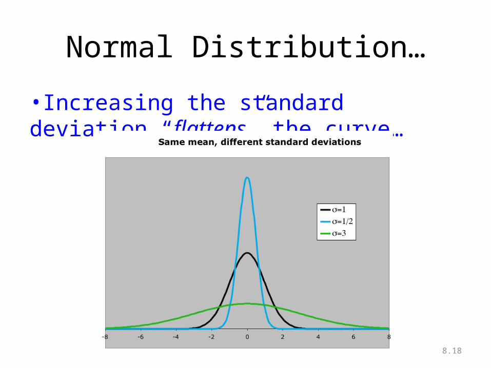
Normal Distribution…

•Increasing the standard deviation “flattens” the curve…

8.19

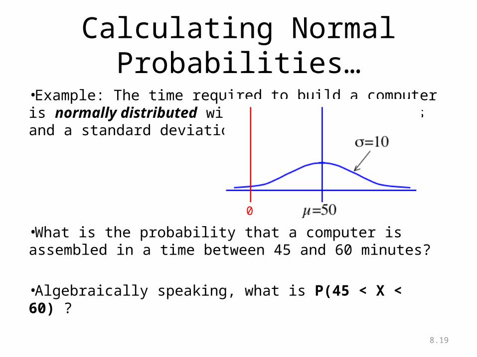
Calculating Normal Probabilities…

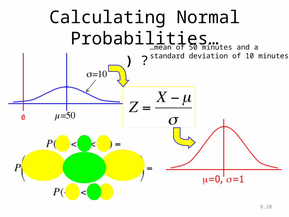
•Example: The time required to build a computer is normally distributed with a mean of 50 minutes and a standard deviation of 10 minutes:

•What is the probability that a computer is assembled in a time between 45 and 60 minutes?

•Algebraically speaking, what is P(45 < X < 60) ?

0

8.20

Calculating Normal Probabilities…

•P(45 < X < 60) ?

0

…mean of 50 minutes and astandard deviation of 10 minutes…

Tripthi M. Mathew, MD, MPH

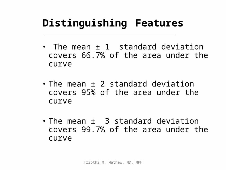
Distinguishing Features

• The mean ± 1 standard deviation covers 66.7% of the area under the curve

• The mean ± 2 standard deviation covers 95% of the area under the curve

• The mean ± 3 standard deviation covers 99.7% of the area under the curve

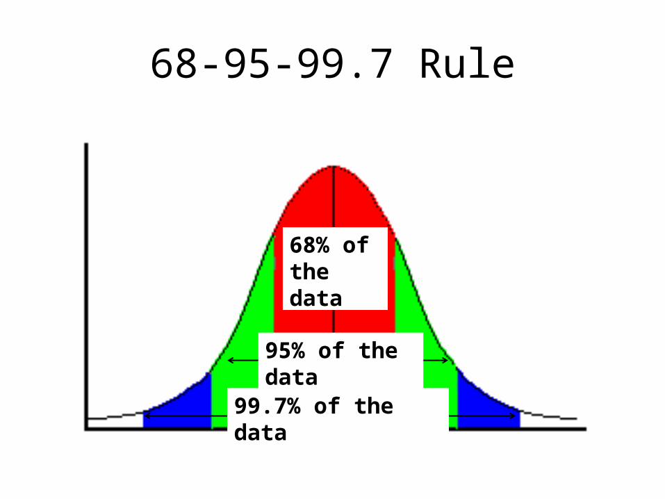
68-95-99.7 Rule

68% of the data

95% of the data

99.7% of the data

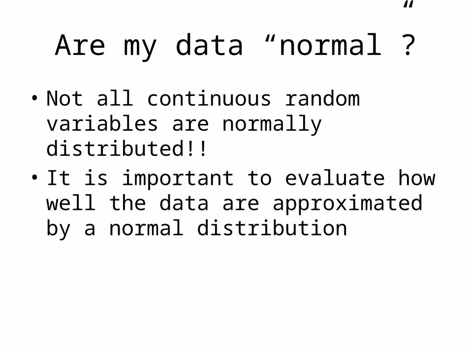
Are my data “normal”?

• Not all continuous random variables are normally distributed!!

• It is important to evaluate how well the data are approximated by a normal distribution

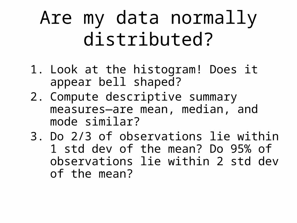
Are my data normally distributed?

1. Look at the histogram! Does it appear bell shaped?

2. Compute descriptive summary measures—are mean, median, and mode similar?

3. Do 2/3 of observations lie within 1 std dev of the mean? Do 95% of observations lie within 2 std dev of the mean?

June 5, 2008Stat 111 - Lecture 7 - Normal

Distribution 25

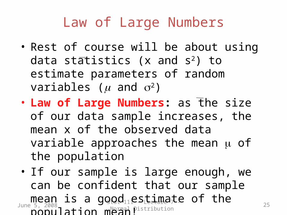
Law of Large Numbers

• Rest of course will be about using data statistics (x and s2) to estimate parameters of random variables ( and 2)

• Law of Large Numbers: as the size of our data sample increases, the mean x of the observed data variable approaches the mean of the population

• If our sample is large enough, we can be confident that our sample mean is a good estimate of the population mean!

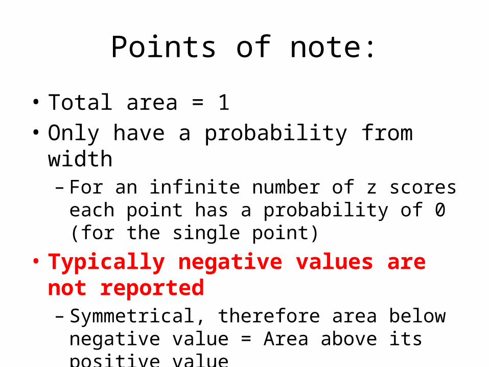
Points of note:

• Total area = 1• Only have a probability from width

– For an infinite number of z scores each point has a probability of 0 (for the single point)

• Typically negative values are not reported– Symmetrical, therefore area below negative value

= Area above its positive value• Always draw a sketch!