


Languages
Pages
Legal


Brigham Young University Brigham Young University
BYU ScholarsArchive BYU ScholarsArchive
Theses and Dissertations
2004-12-13
New Product Launch Decisions under Competition and New Product Launch Decisions under Competition and
Uncertainty: A Real Options and Game-Theoretic Approach to Uncertainty: A Real Options and Game-Theoretic Approach to
New Product Development New Product Development
James O. Ostler Brigham Young University - Provo
Follow this and additional works at: https://scholarsarchive.byu.edu/etd
Part of the Construction Engineering and Management Commons, Manufacturing Commons, and the
Marketing Commons
BYU ScholarsArchive Citation BYU ScholarsArchive Citation Ostler, James O., "New Product Launch Decisions under Competition and Uncertainty: A Real Options and Game-Theoretic Approach to New Product Development" (2004). Theses and Dissertations. 231. https://scholarsarchive.byu.edu/etd/231
This Thesis is brought to you for free and open access by BYU ScholarsArchive. It has been accepted for inclusion in Theses and Dissertations by an authorized administrator of BYU ScholarsArchive. For more information, please contact [email protected], [email protected].

NEW PRODUCT LAUNCH DECISIONS UNDER COMPETITION AND
UNCERTAIANTY: A REAL OPTIONS AND GAME-THEORETIC
APPROACH TO NEW PRODUCT DEVELOPMENT
by
James Owen Ostler
A thesis submitted to the faculty of
Brigham Young University
In partial fulfillment of the requirements for the degree of
Master of Science
School or Technology
Brigham Young University
December 2004

BRIGHAM YOUNG UNIVERSITY
GRADUATE COMMITTEE APPROVAL
Of a thesis submitted by
James Owen Ostler
This thesis has been read by each member of the following graduate committee and by majority vote has been found to be satisfactory
Date Charles R. Harrell, Chair
Date Michael Miles
Date Nile Hatch

BRIGHAM YOUNG UNIVERSITY
FINAL READING APPROVAL
I have read the thesis of James Owen Ostler in its final form and have found that (1) irs format, citations, and bibliographical style are consistent and acceptable and fulfill university and department style requirements; (2) its illustrative materials including figures, tables, and charts are in place; and (3) the final manuscript is satisfactory to the graduate committee and is ready for submission to the university library. Date Approval for the Department
Charles R. Harrell Chair. Graduate Committee
Acceptance for the College
Thomas L Erekson Director, School of Technology
Douglas M Chabries Dean, Ira A. Fulton College of Engineering and Technology

ABSTRACT
NEW PRODUCT LAUNCH DECISIONS UNDER COMPETITION AND
UNCERTAIANTY: A REAL OPTIONS AND GAME-THEORETIC
APPROACH TO NEW PRODUCT DEVELOPMENT
James Owen Ostler
School of Technology
Master of Science
New product development is central to many firms’ future success. Not only as a
means to continue to maintain their piece of the market, but product development can
also be a strategic means for a company to diversify, and/or alter focus to adapt to
changing market conditions.
Most of the research in new product development has been on how to do it
cheaper and faster than the next guy. However, early commercialization does not
guarantee a position of strength in the market. Failures of EMI in CT scanners and Xerox
in personal computers illustrate that being first to market does not ensure success or even
survival. There are two main factors that inhibit managers from making educated

decisions on when to introduce a new product. First, firms do not exist in a vacuum and
any action they take will be countered by their competition. Second, with new products
the only certainty is uncertainty.
To allow such decisions to become “gut feeling” decisions puts a company’s
future at unnecessary risk. This is evidenced by the many firms that have had devastating
results because of poor decisions with regard to launching a new product.
While high level quantitative tools have recently begun to be used to evaluate
corporate strategy, these tools are still mainly confined to research groups within large
corporations. Both real options (to handle uncertainty) and game theory (to capture the
effects of the competitions actions) have been evaluated and used by these groups.
However, they have not been adequately integrated together in the academic world, let
alone in industry. This thesis help bridge the gap between strategic decision making, and
the theoretical world of economic decision analysis creating a prescriptive model
companies can use to evaluate strategically important new product launches.
To bridge this gap a method that is able to handle the integration of game-
theoretic and options-theoretic reasoning to the strategic analysis of new product
introduction is developed. Not only was a method developed that could incorporate the
two methods it was done in a way that is accessible and useful outside of the academic
world.

ACKNOWLEDGMENTS
I would like to thank my committee for their support in my efforts to accomplish
my goals. I would also like to give special thanks to my wife Megan who has supported
me in everything that I do.

viii
Table of Contents
CHAPTER 1. THESIS MOTIVATION AND FRAMEWORK......................................... 1
1.1 Model.................................................................................................................. 2
1.2 Methodology ....................................................................................................... 5
1.3 Problem Statement .............................................................................................. 7
1.4 Delimitations ....................................................................................................... 9
CHAPTER 2. LITERATURE REVIEW .......................................................................... 11
2.1 Importance of New Product Development ........................................................ 11
2.2 Why Develop Products Faster .......................................................................... 12
2.2.1 Quick product development time .............................................................. 12
2.2.2 First mover advantage ............................................................................... 13
2.3 Costs of Speed................................................................................................... 16
2.3.1 Time cost tradeoff ..................................................................................... 16
2.3.2 Competing objectives................................................................................ 17
2.4 Time-to-Market Tradeoff .................................................................................. 20
2.4.1 First-mover disadvantages ........................................................................ 20
2.4.2 Market timing............................................................................................ 20
2.5 New Product Evaluation .................................................................................. 21
2.5.1 Discounted cash flow................................................................................ 21
2.5.2 Real options ............................................................................................... 22

ix
2.5.3 Options and new product development ..................................................... 24
2.6 Competitive Response and Game Theory......................................................... 25
2.6.1 Game theory.............................................................................................. 25
2.6.2 Timing of technology introduction in a duolpoly ..................................... 30
2.6.3 Integrating real options and game theory.................................................. 30
CHAPTER 3. METHODOLGY FOR MODELING THE INVESTMENT DECISION . 33
3.1 Game-Theoretic Analysis ................................................................................. 34
3.2 Real Options Analysis....................................................................................... 39
3.3 Cash Flow ......................................................................................................... 42
3.4 The Demand Model .......................................................................................... 45
3.5 Assumptions...................................................................................................... 51
3.6 Model Programming ......................................................................................... 52
CHAPTER 4. METHODOLGY OF ANALYSIS ............................................................ 53
4.1 Monte Carlo Simulation............................................................................................. 53
4.2 The Hazard Model ............................................................................................ 55
CHAPTER 5. ANALYSIS AND RESULTS.................................................................... 59
5.1 Using the Hazard Model to Make Real Time Decisions .................................. 59
5.2 Real Time Decision Making ............................................................................. 60
5.2.1 Testing hypothesis .................................................................................... 61
5.2.2 Risk management ...................................................................................... 65
5.2.3 Crosstabulation ......................................................................................... 65
CHAPTER 6. CONCLUSIONS AND FUTURE RESEARCH....................................... 69
6.1 Conclusions ........................................................................................................ 69

x
6.2 Future Research........................................................................................................... 70
REFERENCES ................................................................................................................. 71
APPENDIX....................................................................................................................... 77

xi
List of Tables
Table 3-1 – Normal form entry game with a 20 year horizon .......................................... 35
Table 3-2 – Assumed parameters for simulation models.................................................. 51
Table 4-1 – Variable matrix .............................................................................................. 54
Table 5-1 – Boeing survival table ..................................................................................... 63
Table 5-2 – Variables in the equation............................................................................... 64
Table 5-3 – Airbus survival table...................................................................................... 64
Table 5-4 –Variables in the equation................................................................................ 65
Table 5-5 – BL*DO*CIA Crosstabulation ....................................................................... 66
xii
List of Figures
Figure 1-1 – A 2x2 matrix of NPV payoffs ........................................................................ 5
Figure 2-1 – Endogenous generation of first-mover advantages ...................................... 14
Figure 2-2 – The development time cost tradeoff............................................................. 17
Figure 2-3 – Four key product development objectives and six tradeoffs........................ 18
Figure 2-4 –Thee representative forms of a game ............................................................ 29

1
CHAPTER 1. THESIS MOTIVATION AND FRAMEWORK
New product development is central to many firms’ future success. Not only as a
means to continue to maintain their piece of the market, but product development can
also be a strategic means for a company to diversify, and/or alter focus to adapt to
changing market conditions (Schoonhoven, Eisenhardt, & Lyman, 1990).
Most of the research in new product development has been on how to do it
cheaper and faster than the next guy. Manufacturing was usually pushed to find new
ways of producing products faster in the goals of being first to market. However, this
world is not so simple. Early commercialization does not guarantee a position of strength
in the market. Failures of EMI in CT scanners and Xerox in personal computers illustrate
that being first to market does not ensure success or even survival (Teece 1986). Recent
work by Lieberman and Montgomery (1988, 1998) shows that late movers can enjoy
advantages such as: (1) free-riding on the first mover’s investments, (2) technological and
market uncertainty, (3) technological discontinuities, (4) incumbent inertia of the first
mover making it difficult to adapt to change.
A new product’s success also depends on its timing. Abell (1978) introduced the
concept of a “strategic window of opportunity”. Entry which is too late represents lost

2
opportunity; on the other hand, a product introduced to the market too early may not be
received by customers or market channels.
There are two main factors that inhibit managers from making educated decisions
on when to introduce a new product. First, firms do not exist in a vacuum and can be
assured that any action they take will be seen and countered by their competition. Second,
the only certainty in the world of new products is uncertainty.
To allow such decisions to become “gut feeling” decisions puts a company’s
future at unnecessary risk. This is evidenced by the many firms that have had devastating
results because of poor decisions with regard to launching a new product. There are tools
that deal with each of these factors separately. Game theory can help understand
competitors expected response, and real options can deal with the uncertainty of the
market. However, neither of these tools alone will incorporate all of the information
necessary to make an educated decision.
This research joins with the recent work of Smit and Trigeorgis (2001), Smit and
Ankum (1993), and Kulatilaka and Perotti (1998) to add the influence of rivals into real
options analysis of strategic investment and explicitly introduce the resulting tension
between the value of commitment and the value of flexibility in the introduction of new
products.
1.1 Model
For this study the chosen context to explore the dynamics of entry timing choices
is in the market for “very large aircraft” (VLA) aircraft. Boeing has held an unchallenged
monopoly in the VLA aircraft market for almost 40 years with the 747 aircraft. Boeing’s

3
monopoly in the VLA market plays a critical role for the company in two ways: first,
Boeing earns substantial monopolistic profits on their pricing of the 747; second, Boeing
uses these monopolistic profits to subsidize other plane segments where they compete
against Airbus. Recognizing the profit potential from breaking Boeing’s monopoly,
Airbus has repeatedly announced its intention to build the A380, a larger VLA than any
previously built. Airbus’s motivation for entering the market is both to tap the profits in
the VLA segment as well as the competitive advantage of the VLA monopoly position
that Boeing has been enjoying and leveraging.
Boeing’s daring gamble in 1965 launching the 747 jumbo jet was one of the main
reasons that they are the industry leader in the oligopoly market of aerospace
manufacturers, and until Airbus began looking at developing the A380 they enjoyed
monopolistic returns being the sole provider of an aircraft in the super-jumbo jet
category. Now the potential entry of a larger and more efficient aircraft than the 747
Boeing is faced with a critical strategic decision of how to respond to this new entry. If
they do nothing they may lose their position in the aerospace market along with billions
of dollars. On the other hand, launching their own new jumbo jet may not be the answer
since recently failed launches by companies such as the Glenn Martin Company and
Lockheed, have proven devastating. Even the successful launch of the 747 had almost
failed, and Boeing cannot afford to make a mistake that will cost them billions of dollars.
However, entry by Airbus into the superjumbo segment would do considerable
damage to Boeing. The increased size and efficiency of the A380 would likely put
significant competitive pressure on Boeing either reducing margins on the existing 747 or
forcing Boeing to launch a new plane. While Boeing did not have plans to launch a
4
completely new aircraft, it was believed that a revised 747 (with increased efficiency and
seating) could be launched for approximately $2-3 billion. Boeing is concerned with how
the competitive response to either launching or not launching will change what airbus is
planning to do. For example, Boeing needs to know whether the launch of this new plane
would effectively blockade Airbus’ entry.
On the other hand, the decision facing Airbus is very important and complex.
First, the market for intercontinental jumbo jets is predicted to experience significant
growth over the coming decades as traffic on Pacific routes expanded. In addition,
Airbus is under increasing pressures from its customers to provide a full line of aircraft.
However, at the same time, Airbus faces significant risk. The capital investment required
for the project is sizeable; if demand for the plane fails to materialize, the financial
viability of the company could be endangered.
By building a model of the situation, possible outcomes can be explored and
decisions rules found. While the future cannot be predicted perfectly by a model,
different decision policies can be evaluated and then used in the actual decisions that
need to be made. Two economic approaches are used to help understand and breakdown
the problem, game-theory and real options. Both of these approaches can be applied to
the Bertrand Oligopoly situation that arises in the airline industry.
While game theory focuses on the effects resulting from strategic interaction, real
options concerns itself with decision-making under uncertainty. In particular, real
options theory is concerned with decisions where current decisions have implications for
future investment opportunities. In this case the airlines are presented with a buy (launch)

5
or wait scenario. By waiting for more information about future conditions they may
increase their expected return on investment.
1.2 Methodology
In the Boeing-Airbus case the stochastic nature of the demand can be modeled by
a Markov Chain (Benkard 2000). This assumption allows for the model to solve for the
dynamic possibilities instead of stationary situations. However, the payoff that the
airlines will receive is dependent upon more that just the future total demand of the
product because it is also path dependent. This path dependency is caused by the time
value of money and the steep learning curve in building jumbo-jets, where the first few
planes can cost five to six times the cost of the one-hundredth plane (Benkard 2000).
As a practical matter, we can solve the game-theory part of the problem through
the joint use of simulations and a common technique used to solve game theoretic
problems, “backward induction.” For example, under certain assumed conditions, a static
picture of the tradeoff for one decision period is illustrated in Table 1.
Table 1 shows net present value (NPV) profit results of the launch or no launch
options for Boeing and Airbus at their
Nash Equilibrium points. Looking
forward, the game matrix shows
Airbus is always better off launching
regardless of what Boeing decides to
do. This means that Boeing needs to
Boeing
No Launch Launch
No Launch 7,421 12,302
Airbus 0 0 Launch 2,729 2,391 4,132 3,896 Figure 1-1 A 2x2 matrix of NPV payoffs

6
base its their decision on the assumption that Airbus will act rationally and launch.
Consequently, under these conditions Boeing will decide not to launch, despite the fact
that they could make over $12 Billion if they launch and Airbus does not, since doing so
maximizes their profit when Airbus launches.
Traditionally, there are several ways of va luing a real option, such as partial
differential equations, dynamic programming, or Monte Carlo simulations (Dixit and
Pindyck 1994; Trigeorgis 1995). In the Monte Carlo technique, one first generates a
random series of observations according to the estimated distributions of the variables
thought to affect the payoffs of the given investment, and then calculates the cashflows
for each period. One then calculates the net present value of that cash flow stream. By
generating a large sample of such simulated cashflow streams and taking the average of
their net present value, one can arrive at the value of the real option.
Game theoretic reasoning can be incorporated into this analysis by deriving the
optimal strategy for each firm over the entire sequence by utilizing “backward induction”
(Ghemawat 1991). For every random sequence generated, the optimal strategy for the
firm is derived by iteratively determining the optimal strategy at each stage of the “game”
beginning with the final period and working backward. This procedure ensures that each
player takes the optimal action for that particular realization of the random process. By
generating a large sample of such random paths with optimal actions over each path and
calculating the average net present value over the whole sample, one can determine the
optimal strategy / investment decision for the firm. This approach to analyzing such a
decision incorporates both the “commitment” value of the investment as well as its
options value.

7
The assumption that demand is stochastic enables this model to be created.
Demand is assumed to follow a Wiener process with a normal distribution around the last
periods demand realizations occurring at yearly intervals. This creates a Markov Chain
similar to what has been proven to be a good representation the airline industry (Benkard
2000).
The stochastic demand assumption is now inserted into a program that
dynamically sets market share, plane prices, etc depending upon the conditions of
demand and the entry of the two airlines. The program then generates an NPV for each
scenario. The results are captured in two 21x21 matrices, one each for Boeing and
Airbus, with the rows and columns representing the years that Airbus and Boeing enter
respectively as shown in appendix 1. For example cell (3, 5) of the matrix would
correspond to the scenario where Airbus enters in year 3 and Boeing in year 5 for the
demand generated for that realization.
1.3 Problem Statement
Despite the rapid incorporation of game theory and real options into the academic
fields of strategy, operations and corporate finance, little progress has occurred in the
transfer of the resulting analytical tools into practice. Unfortunately none of this research
helps a manager that is drowning in a sea of uncertainty. The few methods of how game-
theoretic and options-theoretic reasoning could be usefully integrated together in the
analysis of strategic decisions that have been developed have taken an approach that is
too academic and theoretical to have any use to a manger under pressure to make a
decision.

8
This study evaluates and develops methods to jointly incorporate game theory and
real options analysis into a decision making tool that a manger can easily, and quickly use
to make real time decisions.
This study evaluates the feasibility of using a Hazard model to predict the optimal
time until launch in a similar way to how a Hazard model is used in fields such as
medicine and insurance that use a Hazard model to predict time until an event such as
sickness or death. The limitations and proper use of Hazard models will be set, and the
validity of using a Hazard model evaluated.
Then a methodology of using either a hazard model or what ever the study finds
to be the best way to evaluate the interface of real options and game theory in new
product introduction decisions will be introduced, validated and the details of how a
manager needing to make a decision can to use this method to make better decisions
given.
In conclusion, this study makes three key contributions.
1. First, it outlines an approach to integrating game-theoretic and options-
theoretic reasoning to the strategic analysis of new product development that
can be used to make real time entry decisions. Over the past twenty years,
these two approaches have exercised increasing influence on the field’s
understanding of strategic choice, but the useful integration of the two
approaches has not occurred.
2. Second, the possible use of a Hazard model for real time predictions is
evaluated. Hazard regression is commonly used and accepted as the way to
9
regress real options. This study will explore whether or not a hazard
regression can then be used to model the probability of the event of optimal
entry for real time decision making.
3. Third, this study develops a method that can be practically implemented by
managers under pressure to make a good decision.
1.4 Delimitations
The model is of a two player game and cannot handle the complexity of multiple
player games. This is typical of game theoretical models. However, in many cases it is a
simple matter to lump the competition together and model them as a single entity without
changing the results of the model beyond reason. Thus, the model will work for general
NPI’s that have similar industry structure and not just VLA’s. Further, the key
contribution of a game-theory/real-option methodology can be applied to not only NPI
but also other decisions that face a real options and game theoretic decision, which
happens to be almost all major decisions

10

11
CHAPTER 2. LITERATURE REVIEW
Literature on new product development is diverse with areas focusing on both the
how and the why. The purpose of this chapter is to provide the necessary background to
enable the reader to understand the importance and direction of new product
development. Major prevalent themes are presented with emphasis of tying the why and
how of product development from a strategic point of view instead of the numerous
possible tactics that can be used.
2.1 Importance of New Product Development
We are in an age where speeding products to market has become paramount to a
firms success. Product lifecycles are now often measured in months instead of years
putting incredible pressure on shortening the product development cycle time. For many
firms the ability to gain and sustain a competitive advantage lies in faster product
development cycle time as new products are increasingly becoming the nexus of
competition in many technology- and R&D-intensive industries (Clark and Fujimoto
1991; Brown and Eisenhardt 1995). Product development is also a strategic means for a
company to diversify, and/or alter focus to adapt to changing market conditions
(Schoonhoven, Eisenhardt, & Lyman, 1990).

12
2.2 Why Develop Products Faster
This section will look at advantages that can be gained and the strategic
motivation of shortening the development time of new product development,
2.2.1 Quick product development time
As a strategic weapon time is an equivalent with money, quality productivity and
innovation as a source of competitive advantage (Stalk 1988). Preston G. Smith and
Donald G. Reinertsein [1991] discuss why a company would want to develop products
faster. They argue that while different companies’ motivations will vary the following are
general principles that drive for fast development time:
1. Increased Sales – Each month that can be cut from development is month that
can be added to its sales. The sales life of the product is not only extended
backwards but forwards in instances where loyalty due to switching costs
creating early momentum allowing the product to remain on the market
longer.
2. Higher Margins – in many products the price a customer is willing to pay is
decreasing as a function of time. Also, the sooner a product is released the
probability of more pricing freedom increases as there is less competition.
These factors allow new products to have higher margins during their early
stages compared to latter more mature market.
3. Surprising the competition – in the dynamic world of new products early
introduction can surprise the competition and change the market conditions.

13
4. Responsiveness to Changing Markets, Styles and Technologies – with the fast
pace of changing technology a strong old line of products can be made
obsolete quite abruptly. If a company can not respond quickly revenue and
reputation can be lost. Styling is also important. Chrysler has recently enjoyed
success because its United States competitors’ vehicles often look dated by
the time that they are introduced to the market. A fast-cycle time leads to
flexibility to take advantage of or minimize the downside of change.
5. Maintain a Market Leadership Position – Many companies are known for
being on the cutting edge of technology and the forefront of their marketplace.
Companies such as Honda, Hewlett-Packard and Sony are seen as trend setters
and customers are willing to follow trends set by these companies and pay
more for their new products. Many companies regard accelerated development
as their core competency.
2.2.2 First mover advantage
One of the forces behind fast product development is the strategic advantage of
being first to market (Stalk, 1988) Figure 2-1 shows a framework that Lieberman and
Montgomery (1988) presented as illustrating how first mover advantages lead to profits.

14
Figure 2-1: Endogenous generation of first-mover advantages.
Lieberman and Montgomery (1988, 1998) present that first mover advantages
come from three primary sources. They would argue that previously mentioned
advantages stem from the following:
1. Technological Leadership – there are two main mechanisms by which
advantages can be gained in technological leadership.
a. Advantages derived from the learning or experience curve where
prices fall with cumulative output. In the 1970 the Boston Consulting
Group popularized the idea of gaining advantages through the learning
curve. By being first to market a company can position itself further
down the learning curve than competitors giving a competitive
advantage in many industries.
Enviromental Change
Firm proficiency First-Mover Opportunity
Luck
Mechanisms for Enhancing First-Mover Advantage
Profits

15
b. Success in Patent or R&D races. In many industries such as
pharmaceuticals the winner of patent or trade secret R&D races is the
first to market securing market position. More recently first movers
have been shown to have an advantage with respect to influencing the
path of dominant design, which is often path dependent due to
switching costs and other factors. (Suarez and Utterback 1995)
2. Preemption of Assets(resources) – the first mover can gain advantage by
obtaining control of existing assets. These assets can be broken down into the
following three areas.
a. Input factors such as natural resource deposits can often be gained at
market prices below the future market evolution inflates them.
b. Location in geographic and product characteristics can be a sustained
advantage if there is limited “room” whether physically or
economically. Often the “bottleneck” of an industry can be controlled
in this way similar to how Coke and Pepsi dominate distribution
channels in the soft drink industry.
c. Plant and equipment advantages can be sustainable when scale
economies can deter entrants
3. Buyer Switching Costs – both switching costs and buyer uncertainty can give
first mover advantages where late entrants must invest extra resources to
attract customers away from the original.

16
2.3 Costs of Speed
It can be very expensive and inefficient to develop products too quickly (Smith
and Reinerstsen 1998). Time is not free. To introduce a product sooner a company has to
be willing to make the tradeoffs for time. These tradeoffs come in many forms such as
inferior product design, increased expenses due to time compression diseconomies of
scale etc.
2.3.1 Time cost tradeoff
Observations have shown that there exists a U-shaped relationship between time
and the total development cost. The typical company is on the right side of the minimum
of this curve. They can easily reduce their costs and time by moving further down the
curve (Gupta, Brockhoff, and Weisenfeld, 1992; Smith and Reinertsen, 1998; Bayus,
1997). While the typical company has this opportunity, most believe that they are
operating on the left side of the minimum (Gupta, Brockhoff, and Weisenfeld, 1992).
Figure 2-2 graphically shows this tradeoff.

17
Figure 2-2: The development time cost tradeoff. Adapted from Bayus (1997)
Bayus (1997) modeled this time cost tradeoff curve and showed that optimal time
to market is really a function of the product and market conditions. Bayus (1997) then
developed a speed-to-market model optimizing new product decisions and the associated
markets, demand, and cost conditions.
2.3.2 Competing objectives.
In the product development process there are multiple objectives that compete
with each other. In order to further one objective another needs to be sacrificed.
Managers have intuitively known and stated this in the common phrase: “Good, fast
cheap … Pick any two” (Bayus 1997). However, the problem is actually more
complicated than this. Figure 2-3 shows four key product development objectives and the
six corresponding tradeoffs (Smith and Reinerstsen 1998).
Developm
ent cost
Development time
Des
ired
bala
nce
Min
cos
t
Typi
cal c
ompa
ny

18
Figure 2-3: Four key product development objectives and six tradeoffs.
In order to balance these objectives managers need to remember that the
overriding objective is not any one of these, nor a specific combination of them, but to
make money. Cost in these models is not just strictly monetary but the opportunity costs
of enhanced product performance, loss of flexibility etc that have an impact on the
bottom line. Optimizing on only one of these tradeoffs will lead to failure. In order to
make good decision, decision rules are needed based on financial markets (Smith and
Reinertsen 1998).
Because of the importance of making good decisions in the face of conflicting
objectives, models have been developed to measure these tradeoffs. The previously
mentioned Bayus model modeled two competitive scenarios. In the first scenario a firm
needs to decide whether to accelerate development to catch a competitor that has recently
Market introduction
date
Product unit cost
Development project
expenses
Product performance

19
introduced a new product. The second scenario is where a firm needs to decide whether
or not to speed development to beat the competition to market.
Cohen, Eliashberg and Ho (1996) developed a product performance and time-to-
market trade off model that showed minimizing breakeven time can lead to premature
product introduction. The model uses a multistage product performance improvement
process of, Design à Process à Market, to study how different resources should be
allocated over the different stages. It also considered the cumulative costs and revenues
of the new product over its entire life cycle. The model mainly focuses on the marketing
aspect of product development and improving product characteristics and performance.
The model shows that often it is better to take time to develop a superior product and
improved product development capability should not and is not always demonstrated by
earlier time to market but always leads to enhanced products.
Some research in new product development has changed its focus from having an
emphasis of speed to market towards the market tradeoff for optimal performance. These
models are representative of this change in focus.
While most of these models examine the external forces that dictate optimal
product development time frames by measuring opportunity costs as product costs they
really are about product positioning. Very little research has been about the costs
associated with the design of the process involved in making the product.

20
2.4 Time-to-Market Tradeoff
Although time-to-market has become a major focus of many large companies,
being first to market and the fastest in development is not always better (Lambert and
Slater 1999).
2.4.1 First-mover disadvantages
Early commercialization does not guarantee a position of strength in the market.
The experiences of EMI in CT scanners and Xerox in personal computers illustrate the
challenges faced by many first movers that failed to earn competitive advantage or even
survive (Teece 1986). Lieberman and Montgomery (1988,1998) point out some first
mover disadvantages. Late movers can enjoy advantages such as: (1) free-riding on the
first mover’s investments, (2) technological and market uncertainty, (3) technological
discontinuities, (4) incumbent inertia of the first mover making it difficult to adapt to
change.
2.4.2 Market timing
A market’s readiness to receive a new product is also not constant. Abell (1978)
introduced the concept of a “strategic window of opportunity”. A new product’s success
depends on its timing. Entry which is too late represents lost opportunity; on the other
hand, a product introduced to the market too early may not be received by customers or
market channels. There are many examples of products that were great success stories in
the 90’s that were first unsuccessfully introduced in the 80’s. A company needs to be
aware of market conditions and in a position to take advantage of opportunities that
present themselves.

21
Upon realizing that being first is not everything, Dacko, Furrer, Liu, Sudharshan
(2001) showed that many markets have rhythms and suggested an approach of matching
product introduction and development to the rhythm of the market. This research shows
that the internal development timing question is partly a function of the market.
2.5 New Product Evaluation
The decision of whe ther or not funding should be allocated for a new product is
almost always justified through a discounted cash flow analysis (DCF). Not only is DCF
a inferior method to evaluate the true value of an investment, the optimal launch date is
dependent upon more than a positive cash flow as previously discussed. Real options can
be used to evaluate the timing of launching a new product under market uncertainty.
2.5.1 Discounted cash flow
Probably the most common project evaluation method is the net present value
(NPV) method. However, NPV and other DCF evaluation methods are recognized to be
inadequate approaches to capital budgeting. This is because they cannot properly capture
the value of flexibility to adapt and revise later decisions in response to unknown market
developments. Unfortunately the only constant in the business world is uncertainty,
making NPV calculations inevitably wrong since NPV calculations make implicit
assumptions creating an “expected scenario” with its respective cash flows.
(Trigeorgis 1995)
Despite its imperfections tradition NPV should not be abandoned. Trigeorgis
(1995) suggests that traditional NPV methods should be expanded to include the option
value of the investment, i.e.,

22
Expanded (strategic) NPV = static (passive} NPV of expected cash flows
+ value of options from active management.
The methods of how to evaluate the value of the option have been thoroughly
debated in recent literature. By using the methods that have been established a more
correct evaluation can be made concerning the value of a project.
2.5.2 Real options
The quantitative underpinnings of options derive from the pricing of financial
options. The Black and Scholes equation (Black and Scholes 1973) formally introduced a
risk free way to price financial options. This equation was derived using stochastic
calculus and partial differential equations. Since then other methods have been explored
because defining a set of partial differential equations may not even be possible, let alone
find a closed form solution when dealing with more typical real life applications such as
when there are multiple options interacting (Trigeorgis 1995).
Various numerical analysis techniques have been developed to evaluate options under
complicated conditions. Trigeorgis breaks these methods into two different numerical
techniques:
1. Those that approximate the underlying stochastic processes directly and are
generally more intuitive
2. Those approximating the resulting partial differential equations.
Monte Carlo simulation (Boyle 1977), various lattice approaches such as Cox,
Ross, and Rubinstein’s (1979) standard binomial lattice method, and Trigeorgis’ log-

23
transformed binomial method all fit into the first category. The second category includes
numerical integration, and implicit or explicit finite difference schemes.
Trigeorgis also lists categories of the common applications of real options. They
are:
1. Option to defer—Management has an option to invest, so it can wait x years
to see if conditions justify the investment. An example is an option to buy
land in real-estate development.
2. Time-to-build or staged investment option—Each stage in an investment can
be viewed as an option on the value of subsequent stages.
3. Option to alter operating scale—Under changing market conditions a firm can
expand, contract, shut down and/or restart.
4. Option to abandon—Permanent termination of operations realizing the resale
value of assets.
5. Option to switch—Outputs can be changed giving product flexibility, or the
same outputs can be produced with different inputs giving process flexibility.
6. Growth options—Where an earlier investment is a prerequisite or a link in a
chain of unrelated products or markets that open up future growth
opportunities.
7. Multiple interacting options—Most real life projects include a collection of
the options listed above.
Common to all real options is the value of deferring a decision. Merton (1998)
points out that:

24
The common element for using option-pricing here is . . . [that] the future is uncertain (if it were not, there would be no need to create options because we know now what we will do later) and in an uncertain environment, having the flexibility to decide what to do after some of that uncertainty is resolved definitely has value (1998: 339).
Even though forecasting techniques are improving, uncertainty is most likely
increasing along with the rapid pace of technology. Thus, the value of using real options
in project evaluation is more valuable than ever before. If a firm is going to be successful
in maximizing their profit of new products it is necessary that they use a real options
approach to capture the value of flexibility under uncertainty.
2.5.3 Options and new product development
New product development already currently utilizes methods that capture the
value of these options.
Pharmaceuticals and other R&D intense industries heavily leverage the time-to-
build option. In fact pharmaceutical companies have failure rates of 90-95 percent of
projects with most ending in the early or middle stages of development (Ittner and Kogut
1995).
Another common use of options thinking is when companies try to mitigate the
risk and problems of new process development is the use of modules. Modularity can
help firms compete by promoting time-pacing (Brown and Eisenhardt 1998), managing
complexity (Baldwin and Clark 1997), enabling economies of substitution (Garud and
Kumaraswamy 1995), increasing firms’ strategic flexibility to respond to environmental
change (Sanchez and Mahoney 1996) and/or more effectively manage the tradeoff of
switching from process development to manufacturing, improving performance (Hatch

25
and Macher 2002). A module is effectively an option on future development and
flexibility. Car and computer companies build “platforms” at an increased cost that allow
for modularity, which can be well understood as real options (Baldwin & Clark, 2000).
Baldwin and Clark (2000) have also assessed the tradeoff of whether the investment to
create modularity in production is worth the additional complexity of the design which is
really just a question of whether the value of the options is greater than the increased cost
of complexity. Mcgrath (1997) has also shown real options are toehold investments
designed to better prepare the investor to meet uncertain events in the future (McGrath,
1997).
2.6 Competitive Response and Game Theory
One of the biggest contributors to market uncertainty is competitor response. By
combining real options with a game-theoretical approach the timing decision can more
fully evaluate when the optimal launch date is, and determine what factors influence
when this date occurs.
2.6.1 Game theory
The first studies of games were done on Oligopoly pricing and production.
Cournot (1838), Bertrand (1883) and Edgeworth (1897) all explored how firms in an
oligopoly would choose pricing and production levels. However, these were seen as
special cases and the not applicable in other circumstances. Von Neumann (1928) then
built upon this work in 1928 when he proved the minimax theorem which has been a
central concept of game theory. Neumann (1944) then collaborated with Morgenstern to

26
publish Theory of Games and Economic Behavior, which was the first time game theory
had been brought into the spotlight.
In 1950 Nash introduced the idea of a non-cooperative solution where each player
maximizes their payoff given the other players’ strategies extending game theory to non-
zero-sum games. A non-zero-sum game acknowledges the possibility that in a 2 player
game both players could win or both could lose. The resulting solution of the players’
strategies is called the Nash equilibrium.
The classic example of this is the prisoners’ dilemma. In this situation there are
two prisoners that are being questioned separately. If they both lie, they get away free.
However, the warden offers a lighter punishment to each if they rat and the other does
not. Unfortunately, the Nash equilibrium leads both to rat, and they both end up worse off
for it.
Using the foundational work discussed game theory has come to dominate much
of modern economics and been widely used in many fields. For example it is used in
biology to predict animal behavior and in law to settle bankruptcy settlements (Fudenberg
and Tirole 1985). In fact, game theory has been widely applied to evolutionary concepts
both in biology and the social sciences to the extent that in the preface to Evolution and
the Theory of Games, Maynard Smith (1982) states, “it has turned out that game theory is
more readily applied to biology than to the field of economic behaviour for which it was
originally designed.”
In Courtney’s (2000) Games managers should play he states that there are five
elements of competitive intelligence that need to be understood in order to create a game
that is an accurate representation of any situation. These five elements of the game are:

27
1. Define the Strategic Issue –What decision are you trying to make and how is it
related to other other internal and external decision
2. Determine the relevant players—Which players will have impact upon the
success of your strategy
3. Identify each player’s strategic objectives—it may or not be profit
maximizing, for example the player may only be after market share, or short
run returns etc
4. Identify the potential actions for each player—with each player’s strategic
motives in mind determine what possible action they might take under the
different circumstances created by the game.
5. Determine the likely structure of the game—Will decisions be made
sequentially, simultaneously, is the game repeated etc
After these five elements are determined market research can provide the payouts for
each scenario and the game evaluated.
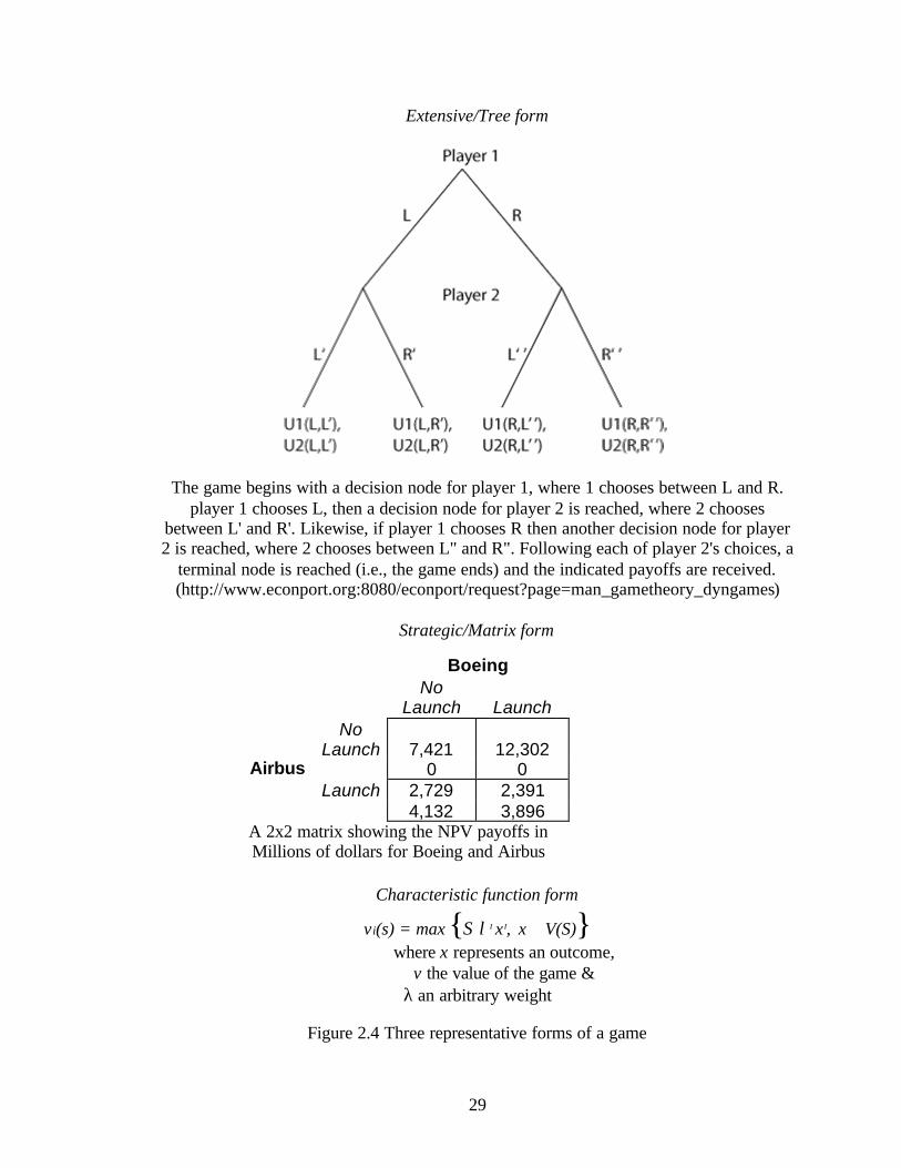
Once the game has been defined it can be represented in any of following three
forms:
1. Extensive or tree form
2. Matrix form
3. Characteristic function form
Each of these forms provides different levels of detail. The extensive form is the
most detailed and consists of a complete formal description of the game played including
sequencing of moves, necessary knowledge at each node, any random occurrences, and

28
the payoffs to each player. The matrix form contains less information, and the
characteristic form the least of all providing only information about the payoffs. A
graphical representation of each of these three forms is provided in Figure 2.4.
29
Extensive/Tree form
The game begins with a decision node for player 1, where 1 chooses between L and R. player 1 chooses L, then a decision node for player 2 is reached, where 2 chooses
between L' and R'. Likewise, if player 1 chooses R then another decision node for player 2 is reached, where 2 chooses between L" and R". Following each of player 2's choices, a
terminal node is reached (i.e., the game ends) and the indicated payoffs are received. (http://www.econport.org:8080/econport/request?page=man_gametheory_dyngames)
Strategic/Matrix form
Characteristic function form
vi(s) = max {Σ λI x I, x ∈V(S)} where x represents an outcome,
v the value of the game & λ an arbitrary weight
Figure 2.4 Three representative forms of a game
A 2x2 matrix showing the NPV payoffs in Millions of dollars for Boeing and Airbus
Boeing
No
Launch Launch
No
Launch 7,421 12,302 Airbus 0 0
Launch 2,729 2,391 4,132 3,896

30
2.6.2 Timing of technology introduction in a duolpoly
Scherer (1967) evaluated the introduction of a product in a duopoly. In his study
the firms were identical and found that if they were required to pre-commit themselves
that they would both enter as soon as possible which was earlier than the optimal time.
Reinganum (1981 a,b) showed that there must be a technology diffusion of
technology forcing the firms to effectively enter on different dates even though they are
identical and there is no uncertainty.
Fudenberg and Tirole (1985) later showed that identical firms that follow a
diffusion process will always be forced to face preemption, and thus force both to equal
payoffs in equilibrium.
2.6.3 Integrating real options and game theory
Smit and Ankum (1993) offered a game-theoretic treatment of competitive
reactions under various market structures using a real options framework. They actual
embed a two player game into each node of a decision tree. However, the more
complicated N-person game has not yet been solved.
Grenadier (1996) developed a equilibrium framework for strategic option exercise
games, focusing on the real estate market. In 2000 Grenadier edited Game Choices: The
Intersection of Real Option and Game Theory, in which he compiles what little work that
has been done in this area. There he states that real options research generally assumes
that the exercising of an option has no effect on the value of other agents’ options and
that assumption is not consistent with reality. Unfortunately, the intersection of these two

31
methodologies is still in their infancy. On the other hand, as Grenadier (2000) states, “It
will be exciting to see the future trajectory of research in this area in the coming years.”
Even since 2000 when grenadier made that statement the rapid incorporation of
game theory and real options has been limited in the transfer of the resulting analytical
tools into practice. Moreover, little attention has been paid to how game-theoretic and
options-theoretic reasoning could be usefully integrated together in the analysis of
strategic decisions (Adner and Levinthal 2004).

32

33
CHAPTER 3. METHODOLGY FOR MODELING THE INVESTMENT DECISION
The traditional method for evaluating the attractiveness of investing in a new
technology or market opportunity for a new product is discounted cash flow analysis.
However, when there are rivals contemplating the same decision, the decisions of one
firm will influence the performance of its rivals in addition to its own performance.
Ignoring the decisions of rivals would likely lead to incorrect estimates of the firm’s
market share, revenues, and discounted cash flows. To explicitly account for the
interdependence between the firms’ decisions, this study constructs a game theoretic
model of the decision to invest in the development and launch a new product. In addition
to the complications of interdependent cash flows, it is common for such a decision to be
fraught with uncertainty. In this case, demand for the new product is assumed to be
unknown and volatile. In the face of this great uncertainty into the model, the model
integrates real options analysis with the game theoretic analysis to make the launch
decision. More specifically, the model measures the value of the option to defer
investment and learn more about the underlying level of demand.

34
3.1 Game-Theoretic Analysis
If the uncertain demand can possibly fall to levels that render the investment
unprofitable, the firm may prefer to delay the launch until a profitable level of demand
can be verified. To accommodate this possibility of deferring investment, the model is
constructed of a two-player (Airbus and Boeing), multi-staged, sequential game for the
game-theoretic element of the analysis. Each firm is restricted to invest and launch its
new product within a fixed time frame (n years) and it is assumed that if either firm has
not entered within that time it has committed to not enter. Therefore, each firm is
independently able to choose to enter in any one of the years in the n-year time frame.
These decisions can be represented in a normal-form game that is constructed in an (n +
1) x (n + 1) matrix (period n + 1 indicates commitment to not launch). This entry game
can be seen as a (2 · n) stage extensive-form game of launch/no launch decisions where
each year is represented in two stages (that year's choices by Airbus and Boeing) of
simultaneous moves. Since firms are not allowed to exit in the game, many branches of
the extensive-form disappear when entry occurs in early stages. For example, if both
firms enter in the first period (stages one and two), the decision in the second period of
whether to launch or not launch is moot. The use of the normal-form game of dimension
(n + 1) x (n + 1) is a collapsing of the complete set of branches down to the feasible set of
branches.
The payoffs for each cell of the (n+1) x (n+1) normal-form game come from
discounted cash flow analysis of that particular launch scenario. To see this, consider the
stylized normal-form game in Table 3.1. The payoffs in cell (2, 4) are ? A¦ 2,4 and ? B¦ 2,4
and result from Airbus' decision to enter in the second period and Boeing's decision to

35
enter in the fourth period. The payoffs are the discounted cash flows derived from the
competition between Airbus and Boeing defined by the specific scenario in each given
year. For example, in cell (2,4) the cash flows (? A¦ 2,4 , ? B¦ 2,4) are constructed assuming
Boeing is a monopolist with the 747 until year two when Airbus invests, then Airbus
competes as a duopolist against the 747 until Boeing invests in the fourth period
afterwhich Airbus competes as a duopolist against the 747X.
When both firms are present in the market, the model assumes that they are
competing in a differentiated Bertrand oligopoly where each firm's revenue is influenced
by the pricing decision of its rival. This implies that every cell of the normal-form game
embeds an underlying, sequential pricing game defined by the oligopolistic competitive
environment in each year.
Table 3-1. Normal form entry game with a 20 year horizon
Airbus Entry Dates
Boeing Entry Dates
1 2 . . . 20 21
1
2
3
. .
.
20
21
( ? A¦ 1 ,1 , ? B¦ 1 ,1 ) ( ? A¦ 1 ,2 , ? B¦1,2 ) . . . ( ? A¦ 1,20 , ? B¦ 1,20) ( ? A¦ 1 , 21 , ? B¦1 ,21)
( ? A¦ 2 ,1 , ? B¦2,1 ) ( ? A¦ 2 ,2 , ? B¦2,2 ) . . . ( ? A¦ 2,20 , ? B¦ 2,20) ( ? A¦ 2 , 21 , ? B¦2,21 )
( ? A¦ 3 ,1 , ? B¦3,1 ) ( ? A¦ 3 ,2 , ? B¦3,2 ) . . . ( ? A¦ 3,20 , ? B¦ 3,20) ( ? A¦ 3 , 21 , ? B¦3,21 )
. . . . . . . . . . . . . . . ( ? A¦20,1 , ? B¦ 20,1) ( ? A¦20,2 , ? B¦20,2 ) . . . ( ? A¦ 1,20 , ? B¦ 1,20) ( ? A¦1,21 , ? B¦1,21 )
( ? A¦20,1 , ? B¦ 21,1) ( ? A¦21,2 , ? B¦21,2 ) . . . ( ? A¦ 2 1 ,20 , ? B¦ 21,20) ( ? A¦21,21 , ? B¦21,21)

36
To model the underlying differentiated Bertrand pricing games, the study begins
by specifying the revenue and cost functions for each firm's annual objective function.
The revenue function in period t for Airbus is
RAt = R(PAt; PBt) (1)
where PAt is the price of the A380 in period t and PBit is the price of the Boeing 747 or
747X (distinguished by the subscript i) in period t. For the sake of solving the Bertrand
pricing game Airbus' cost function is specified in period t as a function of Airbus'
quantity which is a function of Airbus' price:
CAt = C(QAt(PAt)): (2)
Based on the revenue and cost functions, Airbus' problem is to choose the profit
maximizing price in period t:
AtPmax pAt = R(PAt; PBt) – C(QAt(PAt; PBt)) (3)
Deriving the first order conditions of Airbus' problem and solving for Airbus' profit
maximizing price gives us
PAt = rAt(PBt) (4)
where rAt(PBt) is the classic Bertrand reaction function. Because Boeing's price is
embedded in Airbus' revenue function, Airbus' optimal price is an increasing function of
Boeing's price. The reaction function rAt(PBt) gives an infinite set of prices that are
Airbus' best response to all possible prices set by Boeing. The remaining question for
Airbus is where Boeing will set its price. Boeing's profit maximization problem is similar
to that of Airbus:
BtP
max pBt = R(PAt; PBt) –C(QBt(PBt)) (5)
37
Solving for the first order conditions will give Boeing's optimal price as a function of
Airbus' choice of price:
PBt = rBt(PAt) (6)
and using the realized demand for that period.
Since both firms insist on producing on their reaction functions, the only place
that an equilibrium can exist is where the reaction functions cross. This crossing point is
found by solving the system of two equations in two unknowns (rAt(PBt), rBt(PAt)) and
finally obtain the Nash equilibrium pair of prices that are the solution to the pricing game
in period t, (P*At, P*Bt). Substituting these equilibrium prices into each firm's profit
function gives the optimal profit for each firm in period t. Each optimal profit is a single
entry into that firm's discounted cash flow for a particular entry decision.
Of course, to complete the payoff for a cell of the entry game, the equilibrium
prices and resulting profits for every period in the time horizon are needed. Since it is
necessary to populate every cell in the (n + 1) x (n + 1) normal-form game, there will be
very few cases where the competitive environment remains constant throughout the time
horizon. The payoffs for a single cell could comprise periods of monopoly (Boeing 747),
duopoly with A380 and 747, and duopoly with A380 and 747X. Therefore, the payoffs
are the discounted sum of a stream of annual profits based on annual equilibrium prices
and the specific entry conditions of each period. The timing of investment for each firm
defines the particular competitive environment for each year. Every cell in the normal-
form game comprises a sequence of competitive environments defined by the particular
investment timing implied in that cell. Let tA be the timing of Airbus' investment and tB
be the timing of Boeing's investment. Then, the payoffs in each cell are the discounted
38
sum of a stream of annual profits based on annual equilibrium prices and the specific
entry conditions of each period:
? A¦ tA, tB = ∑= +
n
ttr1 )1(
1 [R(P*At, P*Bt¦ t A, tB ) – C (QAt(PAt))] (7)
? B¦ t A, tB = ∑= +
n
ttr1 )1(
1 [R(P*At, P*Bt¦ t A, tB ) – C (QBt(PBt))] (8)
The firms maximize their discounted stream of profits by choosing a series of
Nash equilibrium prices given each particular entry date. This results in optimal
discounted cash flows (? A¦ t A, tB , ? A¦ t A, tB ) that are the payoffs for cell (t A, tB) in the
normal-form entry game.
Having specified the conditional payoffs for each player under all possible
actions, the model determines each firm's strategy. Airbus' strategy is its complete set of
optimal timing decisions in response to Boeing investing in every possible period. For all
tB from period one to (n+1), Airbus' decision is
τ A
max ? A¦ tB=1 (tA) = ∑= +
n
ttr1 )1(
1 [R(P*At, P*Bt , t A¦ tB =1 ) – C (QAt(PAt))]
M M
τ A
max ? A¦ tB=n+1 (tA) = ∑= +
n
ttr1 )1(
1 [R(P*At, P*Bt , t A¦ tB =n+1 ) – C (QAt(PAt))]
The model finds Boeing's strategy in like manner. Given the strategy of each firm,
the model finds the Nash equilibrium for the investment decision by determining which

39
investment dates are simultaneous best responses for Airbus and Boeing. Of course, in
practice there may be no equilibrium or multiple equilibria.
3.2 Real Options Analysis
Traditional approaches to valuing the Airbus A380 project would attempt to
evaluate the discounted cash flows of the project. This study employs the game theoretic
model to overcome the challenge that Airbus’ cash flows will depend on Boeing’s entry
and pricing decisions and Boeing will be similarly influenced by Airbus. However, game
theory alone is not enough to fully model the decision each firm faces because each firm
holds a real option to delay entry to resolve some of the ex ante uncertainty regarding the
size of the market. An integrated model of game theory and real options is required to
make the decision of whether and when to enter. With this integration, the model can
evaluate the entry decision while facing great uncertainty and a competitive rival.
The essence of the value of a real option when facing uncertainty is the
opportunity for the firm to resolve some of the uncertainty before making its irreversible
investment (Copeland and Antikarnov 2001, Dixit and Pindyck 1994, Trigeorgis 1996). If
the firm learns that the uncertain variable will lead to cash flows below a critical value,
the firm will simply not invest (Adner and Levinthal 2004). Thus, in exchange for the
upfront expense of the option, the firm is able to reduce or even eliminate the downside
risk while still preserving the upside risk of the project.
In contrast, traditional net present value analysis assumes that the investment will
happen immediately and makes no allowance for learning of an unprofitable realization
of the uncertain variable. Net present value analysis takes the a priori expectation of

40
uncertain cash flows, including cash flows that lead to negative profits that the firm
would avoid if it could. Therefore, net present value analysis explicitly incorporates the
possibility of unprofitable outcomes while real options analysis explicitly eliminates or at
least reduces the probability of the same unprofitable outcomes. Of course, the value of
the real option relies on the ability to resolve at least some of the uncertainty. If
uncertainty can not be resolved, the real option has no value.
Consider the problem of uncertain demand for superjumbo aircraft. In the unlikely
case that the uncertain demand is known ex ante to be within a range that is high enough
to ensure that both firms can profitably enter, all firms will invest immediately to capture
the early cash flow that would have been lost if the investment were deferred (Smit and
Ankum 1993). In the more likely case that the distribution of the uncertain demand
allows the ex post realizations of demand to fall to levels that earn negative net present
value for at least one firm, the investment decision must include analysis of whether to
defer investment to better learn the realized level of demand. When the true demand is
found to be below the critical value, the project is abandoned and the firm loses only the
cost of acquiring and holding the option to defer. When the true demand is found to be
above the critical value, the firm “sells” the option to defer and invests with certainty, or
at least higher probability, in a profitable outcome. Early on in the specific realization of
demand, the low level and downward trend of demand bodes ill for the project. However,
through the option to delay, demand can be observed to be sufficient to profitably invest.
Combining game-theoretic and real-options approaches is problematic because of
differences in the underlying logic of the two perspectives. For example, game-theory
and real options differ in how they characterize the interrelationships between individual

41
action and the external industry environment. In game theory, current industry conditions
are largely characterized as resulting from the past actions taken by industry players;
while in real options, industry conditions are modeled as the outcome of random
stochastic processes. In other words, industry conditions are endogenous in game
theoretic models and exogenous in real options. Integrating game theory and real options
is made more difficult because payoffs can vary depending upon the actions taken by the
players as well as the realizations of stochastic processes. This aspect of the problem is
not normally featured in real options analysis.
There are several ways of valuing a real option, including partial differential
equations, dynamic programming, and Monte Carlo simulations (Dixit and Pindyck 1994,
Trigeorgis 1996, Schwarz 2002). Given the incompatibility of the calculus of game
theory and the stochastic calculus of real options, the use of Monte Carlo simulation was
the chosen technique. In this technique, a random demand variable is integrated into the
profit function for each firm:
pAt = R(PAt; PBt¦ D0; s) –C(QAt(PAt; PBt)) (9)
pBt = R(PAt; PBt¦ D0; s) –C(QBt(PAt; PBt)) (10)
where D0 is the baseline level of demand (roughly proportional to the intercept of the
demand curve) and s is the variability of annual demand. With the stochastic demand
curve, Airbus' strategy is its optimal choice of entry date for each possible entry date by
τ A
max ? A¦ tB=1 (tA) = ∑= +
n
ttr1 )1(
1 [R(P*At, P*Bt , t A¦ tB =1, Do, s) – C (QAt(P*At , P*Bt))]
M M

42
τ A
max ? A¦ tB=n+1 (tA) = ∑= +
n
ttr1 )1(
1 [R(P*At, P*Bt , t A¦ tB =n+1, Do, s) – C (QAt(P*At , P*Bt))]
Boeing, and Boeing faces a similar problem. Given the stochastic specification of the
demand curve, first a random series of annual demand is generated according to the
specification of demand and then populate the pairs of payoffs for every permutation of
entry dates in the (n + 1) x (n + 1) normal form entry game. The model then finds the
Nash equilibrium pair of optimal entry dates for that particular realization of demand.
3.3 Cash Flow
To perform the simulations of the mathematical model of endogenous entry, a
cash flow model is constructed for each firm, where cash flows depend on the entry
timing and pricing decisions of both firms. First a derived demand model for aircraft is
constructed that assigns market share to each aircraft according to its relative operating
margin on a per seat basis for the airlines. In other words, demand is determined by the
relative cash flow the aircraft generates for its airline customers after covering the
allocated purchase price. Quantity demanded for a particular aircraft is simply determined
by market share times total market demand. Since operating margins depend on price and
on the efficiency of the aircraft being sold, revenue in a particular period changes
depending on the entry decision of the firm. For example, if Airbus has not yet entered
with the A380, Boeing is selling the 747 or the 747X as a monopolist. After Airbus’
entry, quantity demanded will be determined by market shares depending on relative
prices.
Each firm is allowed to enter at any time within a 20 year horizon. Uncertain
market demand fluctuates over the time horizon according to the specification of the

43
uncertainty (in this case demand follows a Markov process). For every realization of
demand, both firms observe a series of annual levels of demand that determine cash flows
that include revenues given from the demand curve, fixed costs determined by the capital
investment, and variable costs determined by a learning curve. Each firm then chooses an
entry date and sets prices for each period in the horizon to maximize its net present value
(NPV).
With the cash flows, the study implements the integrated model of game-theory
and real options as explained above. Airbus and Boeing are ultimately choosing their
optimal entry date conditional on every possible the entry date of the other firm. The
conditional payoffs from these decisions rely on optimal pricing decisions in the specific
competitive environment each year (differentiated Bertrand or monopoly). The Nash
equilibrium pair of entry decisions occurs where both firms are simultaneously choosing
their best response to their rival. This gives the entry timing and payoffs for that
particular realization of demand.
The cash flows for the model are constructed by building the annual profit
functions for each firm given starting demand, relative efficiency of the aircraft, variable
costs, and depreciated fixed costs (capital investment). In any given year where the
competitive environment is a Bertrand duopoly, the model finds each firm’s reaction
function and solve for price. Of course, when Boeing is competing alone the model
solves for the monopoly price. However, Airbus can never act as a monopolist. Even
when Airbus is able to preempt Boeing with its superjumbo, Boeing is still allowed to sell
its incumbent product, the 747.

44
Airbus and Boeing compete over a 44 year time horizon that allows each to enter
as late as period 20, build the project, and fully depreciate its assets assuming 20-year,
straight- line depreciation. At the end of the 44 year horizon, a terminal value for the
project is constructed by assuming that the last cash flow will continue in perpetuity. The
dynamics of the stochastic market demand is defined by a Markov process (random-
walk) with a normal distribution around the demand of the previous period:
dD = s dz (11)
where dD is the change in the level of market demand and dz is an increment to a Gauss
Wiener process with variance s. The random walk has a lower bound for demand of 0.
This is just the obvious result of the fact that Demand cannot be negative. This actually
transforms the data gathered into a form similar to that of a log-normal distribution. Thus
the terminal value given by assuming the last cash flow will continue into perpetuity is
actually a lower value than the true expected value since the median, ~x , and the mean, x ,
of the population of all possible demand paths must always follow the inequality x ≥ ~x .
The only time that x is equal to ~x is when the variance is equal to 0. This fact should
cancel out any worry that the cash flows will not actually continue on into infinity. Any
discrepancies that may occur because of these two facts will not be of a magnitude to
have any biasing of the results
Thus, the total demand expectation at period i, can be seen as a sum of
independent random variables, Xi, with a starting value for the mean equal to current
demand, where X is approximated by a normal distribution. Thus, the sum of Xi‘s can be

45
shown to be normal with a variance of n. This shows that the variance grows linearly
with time and thus the standard deviation grows as the t .
3.4 The Demand Model
The construction of the demand model is crucial for the determination of cash
flows, so a full description of it is included here.
Since there has never been an alternative to the Boeing 747 in the VLA segment
of the aircraft industry, historical data can not be relied upon to estimate a demand curve
after Airbus and Boeing launch their new aircraft. Instead, the model employs a derived
demand model for the VLA segment that determines market demand and allocates market
share to each aircraft based on its contribution to customer profitability. More
specifically, market share is determined by the operating margin per seat that the aircraft
delivers to airlines relative to the margins from other aircraft options. Demand for
specific aircraft is then determined as the product of market share times total demand. To
allow market demand to change with changes in prices (and provide slope to the demand
curves), a “demand shift factor” is constructed that rescales total demand up or down
depending on an industry composite margin given the various aircraft in the market,
depending on the specific scenario being tested, relative to the margin earned during the
prelaunch condition of Boeing 747 as a monopolist. In other words, the known demand
for the Boeing 747 at historical prices is used as an anchor and allows total demand for
jumbo aircraft to change as the composite contribution margin of the aircraft in the
market changes when relative prices change.

46
To construct the demand curve, let the price per seat of an aircraft be given by Psi
where i indicates the type of aircraft where each type has a given number of seats.
Revenue per seat mile assumes an industry average ticket price per passenger and is
therefore constant across aircraft, Rsm = R = $0.116. Variable expense per seat mile begins
with the industry average of $0.06 and which is then rescaled by an operating expense
factor for the particular aircraft. For example, the Airbus A380 is expected to incur only
80% of the variable costs per seat mile of a Boeing 747 due to the A380's superior design
and resulting efficiency. The variable cost per seat mile, as influenced by the efficiency
factor is Vsmi = V ·Ei = 0.06Ei where Vsmi is variable cost per seat mile for aircraft i, V is the
industry average variable cost, and Ei is the efficiency factor for each aircraft. In the
notation, EB7 = 1.0 is the efficiency factor for the Boeing 747 and EA = 0.8 is the
efficiency factor for the A380. Efficiency of the Boeing 747X is denoted as EBX and is
allowed to vary between 0.8 and 1.0 in the analysis. Fixed cost per seat mile begins with
the industry average fixed cost per seat mile (F = $0.045 per seat mile) which is then
rescaled according to the price per seat of the particular aircraft relative to the price per
seat of a 747. This gives a fixed cost per seat mile for each aircraft of
Fsmi = F·Psi / Ps0 = 0.045·Psi/$0.36 where Psi is the price per seat of aircraft i and Pso =
$0.36 is the price per seat of a 747 before any entry decisions by Airbus (pre- launch price
per aircraft for a 747 is $150M). Taking all of these conditions together, an airline's
expected margin per seat for a particular aircraft is simply revenue per seat mile less
variable and fixed costs per seat mile, Mi = R – V – Ei – Fi = R – V – Ei – F·Psi / Ps0.
Total demand and market share for a specific aircraft are both ultimately
determined by the relative margins earned by the airlines. First the market share for each

47
firm is constructed based on relative customer margins. It is then assumed that each
aircraft will sell according to the margin it contributes to customers as a fraction of the
sum of the margins in the market. Thus market share for aircraft i is given by MSi = Mi /
(MA+MB) where MA and MB are the margins of the A380 and Boeing's aircraft
respectively. To get demand for each aircraft, market share must be applied to the total
market demand. We can draw upon relative margins to determine the total market
demand as a function of prices since customer margins depend on aircraft price. To allow
total market demand to vary based on price, the market demand shift factor (DS) is
constructed as a function of market shares which depend upon prices, for each of three
situations:
DS = 0 if Mi = 0 for i = A,B (12)
DS =
+
0
2
M
BMAMβ
if Mi > 0 for i = A,B (13)
DS = ( )
0
,max
M
BMAMβ
if Mi > 0 and Mj = 0 (14)
where M0 is the margin earned by airlines buying a 747 in the prelaunch stage.
Incorporating the market demand shift factor, it is found that total market demand is the

48
known market demand from the prelaunch stage (Q0) times the demand shift factor, Q =
Q0 · DS where Q is total market demand.
With these elements, the demand curve is constructed for each aircraft in each
possible launch scenario. Beginning with simplest case: Airbus does not launch and
Boeing does not launch (NL-NL). In this case, Boeing continues as a monopolist in the
VLA segment producing the 747. As a monopolist, Boeing's individual demand is also
the market demand. The demand curve is given as the premarket quantity times the
demand shift factor as defined in equation (10) where, without an aircraft, Airbus delivers
a margin of $0:
QB7 = Q = Q0
β
07
MBM
= Q0
β
−−
00
7
MsPsBFP
VR
(15)
The demand curve for the case where Airbus does not launch and Boeing does launch
(NL-L) is similar because Boeing is still a monopolist:
QBX = Q = Q0
β
0MBXM
= Q0
β
−⋅−
00
MsPsBXFP
XEVR
(16)

49
When Airbus launches and Boeing does not launch (L-NL), there is a duopoly
structure with Airbus selling the A380 and Boeing selling the 747. In this case, market
demand is determined using the demand shift factor in equation (9):
Q = Q0
+
0
2
M
BMAMβ
= Q0
β
+−−−
0
20
2
M
sPsAFPsAFP
VAVER
(17)
Firm demand for Airbus and Boeing is given by market share multiplied by market
demand:
QA = Q · MSA
= Q0
β
+−−⋅−
0
20
72
M
sPsBFPsAFP
VA
EVR
+−−−
−−
0
72
0
sPsBFPsAFP
VAVER
sPsAFP
AVER
(18)
QB = Q · MSB
= Q0
β
+−−⋅−
0
20
72
M
sPsBFPsAFP
VA
EVR
+−−−
−−
0
72
0
7
sPsBFPsAFP
VAVER
sPsBFP
VR
(19)

50
When both Airbus and Boeing launch (L-L), there is a duopoly structure with
Airbus selling the A380 and Boeing selling the 747X. In this case, market demand is
determined as before:
Q = Q0
+
0
2
M
BXMAMβ
= Q0
β
+−−−
0
20
2
M
sPsBXFPsAFP
XV
AVER
(20)
Firm demand for Airbus and Boeing is given by market share times market demand:
QA = Q · MSA (21)
= Q0
β
+−−−
0
20
72
M
sPsBFPsAFP
XVE
AVER
+−−−
−−
0
72
0
sPsBFPsAFP
XVEAVER
sPsAFP
AVER
QB = Q · MSB (22)
= Q0
β
+−−−
0
20
2
M
sPsBXFPsAFP
XVE
AVER
+−−−
−−
02
0
sPsBXFPsAFP
XVEAVER
sPsXFP
XVER

51
3.5 Assumptions
There are a variety of variables in the model of firm profits that are unknown. For
example, we can estimate Boeing’s discount rate as its weighted cost of capital, but
Airbus is a consortium of companies with headquarters in Europe and does not report the
data needed to compute its weighted cost of capital. Similarly, it is widely acknowledged
that aircraft variable costs follow a learning curve but we would need internal cost and
output data to estimate learning curves for earlier aircraft models. Of course, there is no
guarantee that the new aircraft would follow the learning curves of prior models. Other
relevant variables include the baseline level of demand measured as the units sold over 20
years, SG&A, capital investment of each firm, relative efficiency of each aircraft, and the
corporate tax rate. To find information to improve the assumptions, information was
collected from Airbus’ and Boeing’s websites and from trade journals. The initial
assumptions are listed in table 3-2.
Table 3-2. Assumed parameters for simulation model Variable Value Units Source Starting Demand (D0) Efficiency – 747 Efficiency – 747X Efficiency – A380 Investment – A380 (CIA) Investment – 747X (CIB) Discount Rate – Airbus Discount Rate – Boeing Learning Rate – 747X Learning Rate – A380 Initial VC 747 Initial VC 747X Initial VC A380 Corporate Tax Rate Depreciation SG&A
1000 100% 100% 80% $10,000 $4,000 14.0% 13.8% 82% 82% $500 $500 $500 35% 5% 3%
Units/20 years Percentage Percentage Percentage Millions Millions Percentage Percentage % Cost Reduction % Cost Reduction Millions Millions Millions Percentage Annual % % of Revenue
Ave of published projections Baseline value Assumption Published Reports Ave of published reports Ave of published reports Assumption WACC Assumption Assumption Assumed starting cost Assumed starting cost Assumed starting cost Average US tax rate 20-yr straight line Assumption

52
3.6 Model Programming
The model was programmed into both Mathematica and C. Mathematica was used
for the symbolic derivations, and C was used to computationally crunch the numbers of
each realization of the model. Due to the high volume of realizations required for a
proper Monte Carlo simulation the C program was compiled and run on the
supercomputer Mary Lou.

53
CHAPTER 4. METHODOLGY OF ANALYSIS
4.1 Monte Carlo Simulation
After repeatedly generating realizations of the random demand variable and
finding the Nash equilibrium entry dates, we take the expectation of the ent ry date and
payoffs of the entry decision for the whole. By generating a large enough sample of such
simulated entry dates and payoffs, we find a close approximation of the expected value of
the real option to defer investment given the specification of demand.
In many cases, such as the starting variable cost of the 747, inside knowledge
from the firms would ensure that the assumptions are correct. In many other cases, such
as the starting variable cost of the 747X, even the firms do not know the correct
assumptions a priori. For example, we start with the assumption that the cost of the A380
project will be $10B. However, Airbus acknowledges that the precise cost of the project
is unknown and is expected to fall within the range of $7-15B.
We have already discussed the uncertainty surrounding demand and it is likely
that the operating efficiency of the finished aircraft will vary from initial projections
which will influence demand in turn. Since the optimal entry decisions will surely depend
on the realization of these unknown parameters, it is natural for the decision-maker to test
the sensitivity of entry dates and the option value of delay to changes in the critical

54
assumptions of the model. This is done by varying the assumptions within relevant ranges
and determining the optimal entry timing in the integrated game-theoretic real-options
model for every permutation. This affords the decision-maker a view of the impact of the
unknown variables on the optimal decision. This sensitivity analysis also allows us to test
the hypotheses regarding how these variables influence equilibrium outcomes and the
option value of delay.
A total of 900 runs of 1,000 realizations each were run creating a total of 900,000
data points for statistical analysis. Table 4-1 shows the variables changed for these runs
and the levels for each. The 900 runs come from the permutations of all these levels.
Table 4-1. Variable matrix
s D0 CIB CIA
Efficiency
747X
0.05 500 $2 B $6 B 100%
0.1 700 $3 B $8 B 0.8
0.15 900 $4 B $10 B
0.2 1100 $12 B
0.25 1300 $14 B
1400
The Monte Carlo simulation appropriately integrates the game theory and real
option components of the decision, and the data produced are valuable and can be
analyzed at this point in a myriad of different ways.

55
4.2 The Hazard Model
A hazard model is used to find the probabilities of entry for a firm. A hazard
model is just the conditional probability of an event happening, given it hasn’t already
occurred. In this case it is the probability of entry given that the firm has not already
entered. Hazard analysis has been used to evaluate investment decisions in the
pharmaceutical industry by looking at the time to a second patent. (McGrath 2004) This
study uses hazard rates in a similar way looking at the time to investment being the time
to launch the new product.
A hazard rate is the conditional probability of exercising an option (Kogut 2004),
so using the hazard function gives a way of evaluating the option from a manager’s
decision of do I launch today given the level of demand he sees, the variance in his
demand forecast, etc.
A Hazard function also incorporates information on both censored and
uncensored cases, i.e., whether or not a launch decision is made. This allows information
to be gathered by those cases that no decision is made, since a “no” decision is as much a
decision as a “yes” decision. This insures that we are using all of the information
available increasing the validity, and accuracy of the model.
The intuitive definition of a Hazard is that is just the PDF divided by one minus
the CDF:
( )( )xF
xf−1 (23)

56
However, the more accurate, definition is: If T is the duration since the first
opportunity to launch occurred, then the instantaneous (hazard) rate of the firm launching
at time t is defined as
( )t
tTttTtth
ot ∆
≥∆+<≤=
→∆
}Pr{lim
(24)
In using this definition hazard rates are not probabilities. Because of their
uniqueness, Allison (1995) points out that there are three points have to be understood in
order to properly interpret any given hazard function and its parameters. They are:
1. Even though it is helpful to think of a hazard as an instantaneous probability,
it is not a true probability and its’ hazard can be greater than 1.0.
2. Because a hazard is defined in terms of probability, it is itself an unobserved
quantity. In other words we may only estimate the hazard.
3. Hazards are characteristics of individuals, not populations or samples. Each
individual will have a different hazard given its’ conditions and current state.
Since a hazard is not a probability, the way of interpreting it is as a rate, or the
number of occurrences per interval of time. So in our case, a hazard of .6 would mean
that in that given year a launch will occur .6 times. If the rate is 1.4, a launch will occur
1.4 times. This may be a little confusing in our situation, but think of the hazard to catch
a cold. It may easily be 3.5 for a time period of a year. However, that does not mean that
it is guaranteed that you will catch a cold, and you may catch more than 3.5 over the year.

57
In the case of a product launch, the event can only occur once, but the chances increase
with the hazard. In general, a .63 hazard can be interpreted to be a 63% chance of the
event, but it is still necessary to understand where that comes from and why the hazard
may be greater than 1.0.
The hazard rate is modeled using semiparametric Cox models (Cox, 1972;
Kalbfleisch and Prentice, 1980; Allison, 1995). The equation that we estimate takes the
following specification:
hi(t) = ?0(t)exp{ß1Xi1 + ... + ßkXik} (25)
where h(t) is the hazard rate of the launch event. ?(t) is an unspecified baseline rate for
the transition. Xik’s are time-constant covariates and the ßk’s are unknown regression
parameters. Because ?(t) is an unspecified step function, the Cox model is an extremely
flexible method for modeling time dependence (Sørensen and Stuart, 2000).

58

59
CHAPTER 5. ANALYSIS AND RESULTS
Once the Monte Carlo simulation has generated the data, a statistical software
package can be used to perform the Cox Regression. Almost all modern statistical
software packages offer a hazard regression option that includes a Cox Regression. For
the purpose of this study SPSS was the statistical software package chosen to analyze the
data produced by the Monte Carlo simulation.
5.1 Using the Hazard Model to Make Real Time Decisions
The Hazard model approach can accurately show the influence that different
variables have on the decision either separately or with respect to each other.
However, in the use of a hazard model to either regress or to a model decision making
there is one major assumption that needs to be made that either current real options
literature is unaware of or chooses to ignore. This assumption is that the firm making the
decision always makes the right decision. The reason that this assumption is necessary
can be shown by comparing the way the model evaluates a decision as opposed to the
classical use of a hazard model to regress and predict the probability of death. In the first
period of the model the scenarios both perform in the same way. Unfortunately, after the
first period ends the two models diverge in what is being measured and/or predicted.

60
This problem only occurs in real time decision making. The hazard model can
regress another model such as the one built for this study since the right decision is
always made, or in other words just as in death the outcome is not based on a decision,
but an actual outcome. Unfortunately the second that you try to apply the model to
predict actual decision making behavior the assumption of absoluteness of a correct
decision is violated.
Thus, rather than develop a method to evaluate real options in real time using a
hazard model this study has shown that the hazard model has been inappropriately used
in recent strategy and decision analysis research to model and evaluate real decisions. For
example, the McGrath study of time until a second patent in the pharmaceutical industry
assumes that not only was the correct decision made in the filing for the first patent, but
that all related decisions in between the two patents also satisfy the assumption of
optimality. While this does not eliminate all value of hazard analysis for evaluating real
options, it does force an assumption that calls any results in to serious question. Until
another tool is developed real options researches may have to settle for a suboptimal way
to evaluate real options, but since the error introduced is independent and unique for
every study results will have to be taken at face value and study comparisons avoided.
5.2 Real Time Decision Making
Fortunately this study has developed a method to evaluate both real options and
game theory in the forward looking world of predictive models. This is possible without
using a hazard model since the original model that this study has developed
endogenously captures the real option value to delay as well as game theoretical
dynamics. In fact, in losing the ability to use a hazard model, the only real loss is in the

61
ease that a decision can be reached. In reality, by not fitting the original data to another
model but instead basing the decision off of the original data, no information is lost from
the data resulting in a model with more accurate predictive power. A decision maker can
go directly to the model to evaluate different decisions.
While many less sophisticated managers may not feel comfortable using and
interpreting the results of the model directly, it is not unusual that for highly important
strategic decisions, such as important new product launches, many different divisions
within a company are sought out for their input, and in most major corporations analysis
at a similar level of complexity is routinely performed by either an internal or external
consulting team or captured into a software package. Complicated forecasting is already
performed in almost all situations and this type of analysis is a natural extension of
forecasting that should be welcomed by the “Geek Groups” that seem to inhabit this
domain.
5.2.1 Testing hypothesis
Hazard regression has the ability to regress over multiple sets of data and give
time dependency to the decision, but can also be done as a straight regression with no
other variables other than event time and give you the baseline. This flexibility allows a
modeler the ability to run various scenarios without having to worry about the underlying
methods feasibility which could possibly require changing the regression format.
The equation will not predict the optimal time to launch. It will however help a
manager make his decision in whether or not he should launch in a real time decision. For
example, an Airbus manager can plug into the equation that Boeing has or has not already

62
launched the 747X. However, what constitutes credible commitment on Boeing’s part is
up to interpretation. This is further complicated since it can be shown that Boeing prefers
to delay the launch of Airbus even if it means that they do not launch because of their
current monopolist position in the market. Thus, a manger for Airbus would need to
evaluate the model under both situations, determining what his choice would be given the
two scenarios, and then make a judgment on what the best course to follow is given the
circumstances.
Following this logical process, a manager can test hypotheses that he has with
regard to whether and to what degree a variable influences the firms decision to launch or
not. A manger can even look at what a competitor’s action would best suit them and then
try to “change” or distort what they see to try and create that scenario.
Table 5-1 is a Survival table for Boeing under all conditions run in the simulation.
In the table the baseline of the Hazard Model is shown, and well as the results when
plugging in the mean of the different variables into the equation regressed. Table 5-2
shows the different variables regressed and their respective significance and regression
equation coefficients, and the 95% CI for each. As you can see all variables selected for
this regression were statistically significant at the most stringent of confidence levels. In
fact the significance for many of them was so high that the value of significance was
essentially 0, signifying a 100% confidence of significance.
Tables 5-3, 5-4 are the same tables as shown for Boeing but now run for Airbus.
If you look at the corresponding variables you can see how the same variable can have
either the same or opposing effect on the two firms. For example, the variable of
efficiency, which represents the efficiency for the 747X, pushes Boeing to an earlier

63
launch, but inhibits Airbus from launching under the general parameters regressed. On
the other hand, demand (launchBD or launchAD) which has the same input to both
pushes both towards a launch decision.
Using Hazard Regression in this way a manager can see what factors effect his
decision and how they change under the different scenarios that he wishes to evaluate.
Table 5-1. Boeing survival table Time Baseline Cum Hazard At mean of covariates Survival SE Cum Hazard 1 0.708594573 0.715715 0.000304 0.334473472 2 0.823535151 0.677919 0.000381 0.388728155 3 0.903764006 0.652726 0.000425 0.426598081 4 0.957159053 0.63648 0.00045 0.451801812 5 1.026654477 0.61594 0.000479 0.484605303 6 1.088723788 0.598156 0.000502 0.513903492 7 1.147454964 0.581801 0.00052 0.541626002 8 1.204152397 0.566437 0.000537 0.568388537 9 1.252379472 0.553689 0.000549 0.591152863 10 1.320428459 0.536186 0.000564 0.623273601 11 1.383713316 0.520406 0.000577 0.653145557 12 1.442969814 0.506052 0.000587 0.681116032 13 1.504245027 0.491625 0.000596 0.710039388 14 1.567947125 0.477062 0.000605 0.740108292 15 1.635587919 0.462071 0.000612 0.772036353 16 1.698125005 0.448631 0.000618 0.801555344 17 1.769279973 0.433813 0.000623 0.835142179 18 1.8650879 0.414631 0.000629 0.880365797 19 2.045820746 0.380726 0.000632 0.965675993 20 3.473041662 0.194105 0.000475 1.639358171

64
Table 5-2. Variables in the equation
B SE Sig. Exp(B) 95.0% CI for Exp(B)
Lower Upper Eff 0.521328 0.015289 0 1.684263 1.634541 1.735498 StDev 0.004437 0.000189 0 1.004447 1.004074 1.004819 CIB -0.00029 1.67E-06 0 0.99971 0.999707 0.999713 AbB -3.09169 0.004791 0 0.045425 0.045001 0.045854 launchBD 0.025491 6.19E-05 0 1.025818 1.025694 1.025943
Table 5-3. Airbus survival table Time Baseline Cum Hazard At mean of covariates Survival SE Cum Hazard 1 1.415859935 0.773891 0.000273 0.256324805 2 1.569093785 0.752717 0.000335 0.284065993 3 1.704650833 0.734469 0.000382 0.308607004 4 1.808000319 0.720855 0.000415 0.327317214 5 1.949789307 0.702587 0.000454 0.352986444 6 2.096149656 0.684215 0.000491 0.379483266 7 2.220295631 0.669009 0.000519 0.401958436 8 2.355328482 0.652852 0.000546 0.426404547 9 2.474735714 0.638891 0.000569 0.448021823 10 2.636902207 0.620407 0.000595 0.477380161 11 2.809171879 0.601356 0.000621 0.508567561 12 2.979067748 0.583142 0.000642 0.539325212 13 3.149059417 0.565469 0.000662 0.570100206 14 3.331346042 0.547112 0.00068 0.603101058 15 3.495819305 0.531062 0.000694 0.63287701 16 3.683879749 0.513285 0.000708 0.666923144 17 3.871430735 0.49615 0.00072 0.700877046 18 4.091854431 0.476741 0.000732 0.740782166 19 4.387089731 0.451929 0.000744 0.794231048 20 5.550849898 0.366075 0.000737 1.004916152
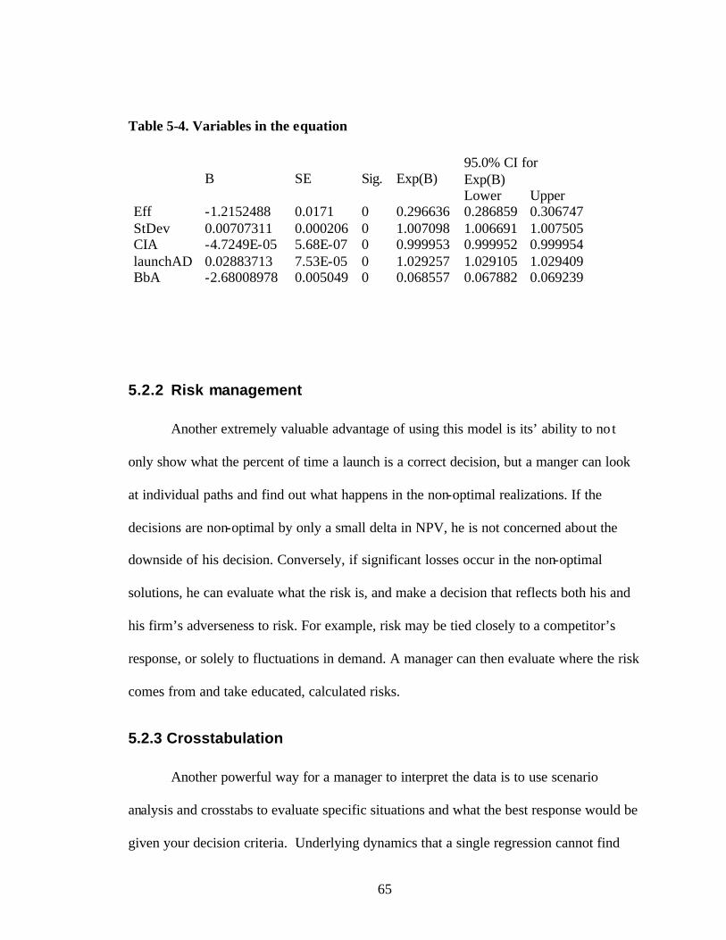
65
Table 5-4. Variables in the equation
B SE Sig. Exp(B) 95.0% CI for Exp(B)
Lower Upper Eff -1.2152488 0.0171 0 0.296636 0.286859 0.306747 StDev 0.00707311 0.000206 0 1.007098 1.006691 1.007505 CIA -4.7249E-05 5.68E-07 0 0.999953 0.999952 0.999954 launchAD 0.02883713 7.53E-05 0 1.029257 1.029105 1.029409 BbA -2.68008978 0.005049 0 0.068557 0.067882 0.069239
5.2.2 Risk management
Another extremely valuable advantage of using this model is its’ ability to no t
only show what the percent of time a launch is a correct decision, but a manger can look
at individual paths and find out what happens in the non-optimal realizations. If the
decisions are non-optimal by only a small delta in NPV, he is not concerned about the
downside of his decision. Conversely, if significant losses occur in the non-optimal
solutions, he can evaluate what the risk is, and make a decision that reflects both his and
his firm’s adverseness to risk. For example, risk may be tied closely to a competitor’s
response, or solely to fluctuations in demand. A manager can then evaluate where the risk
comes from and take educated, calculated risks.
5.2.3 Crosstabulation
Another powerful way for a manager to interpret the data is to use scenario
analysis and crosstabs to evaluate specific situations and what the best response would be
given your decision criteria. Underlying dynamics that a single regression cannot find
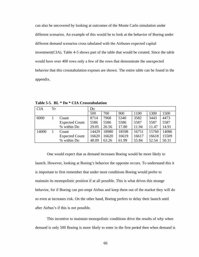
66
can also be uncovered by looking at outcomes of the Monte Carlo simulation under
different scenarios. An example of this would be to look at the behavior of Boeing under
different demand scenarios cross tabulated with the Airbuses expected capital
investment(CIA). Table 4-5 shows part of the table that would be created. Since the table
would have over 400 rows only a few of the rows that demonstrate the unexpected
behavior that this crosstabulation exposes are shown. The entire table can be found in the
appendix.
Table 5-5. BL * Do * CIA Crosstabulation CIA Yr Do 500 700 900 1100 1300 1500 6000 1 Count 8714 7968 5340 3582 3443 4473 Expected Count 5586 5586 5586 5587 5587 5587 % within Do 29.05 26.56 17.80 11.94 11.47 14.91 14000 1 Count 14429 18980 18598 16751 15760 14086 Expected Count 16620 16620 16619 16617 16618 15509 % within Do 48.09 63.26 61.99 55.84 52.54 50.31
One would expect that as demand increases Boeing would be more likely to
launch. However, looking at Boeing’s behavior the opposite occurs. To understand this it
is important to first remember that under most conditions Boeing would prefer to
maintain its monopolistic position if at all possible. This is what drives this strange
behavior, for if Boeing can pre-empt Airbus and keep them out of the market they will do
so even at increases risk. On the other hand, Boeing prefers to delay their launch until
after Airbus’s if this is not possible.
This incentive to maintain monopolistic conditions drive the results of why when
demand is only 500 Boeing is more likely to enter in the first period then when demand is

67
triple that at 1500. This occurs because Airbus will never enter into the market that has
Do at 500 if it has to compete against Boeing to do so. Thus, when Boeing preempts
Airbus at low demand they are almost completely assured of maintaining their
monopolistic position. The chances of Boeing preempting and keeping Airbus out of the
market decrease with higher demand. This is represented by Boeing’s increasing
reluctance to launch as demand increases. This reverses slightly once demand reaches
1500 since at that point the high level of demand starts to outweigh the loss of an Airbus
entry, and since Airbuses decision becomes increasingly independent of Boeing’s
decision. Also, the value of waiting is demonstrated in all cases by lower than expected
launch rates.
A similar argument follows for when CIA is 1400, except here the factor limiting
Airbus from launching is its high investment cost. Thus, Boeing can easily preempt,
shown by more frequent launches. At the same time the importance of demand in keeping
Airbus out is diminished so Boeing reacts more as expected to demand, where its
probability of launching is positively related with demand. This effect changes however
as demand increases beyond a point where CIA becomes decreasingly strong as an
incentive to not launch.

68

69
CHAPTER 6. CONCLUSIONS AND FUTURE RESEARCH
6.1 Conclusions
While high level quantitative tools have begun to be used to evaluate corporate
strategy, these tools are still mainly confined to research groups within large
corporations. Both real options and game theory have been evaluated and used by these
groups. However, they have not been adequately integrated together in the academic
world, let alone in industry. This thesis help bridge the gap between strategic decision
making, and the theoretical world of economic decision analysis creating a prescriptive
model companies can use to evaluate strategically important new product launches.
To bridge this gap a method that is able to handle the integration of game-
theoretic and options-theoretic reasoning to the strategic analysis of new product
introduction is developed. Not only was a method developed that could incorporate the
two methods it was done in a way that is accessible and useful outside of the academic
world.
In developing this methodology the fallacy of using a hazard model to evaluate
decision making such a real options approach was discovered. Stricter and more
unrealistic assumptions are required to use hazard regression than has previously been

70
acknowledged. This thesis not only discovered these assumptions but also explained their
limitations and when it hazard regression can still be a useful tool.
The study also demonstrates how optimal behavior is often counterintuitive when
decisions are influenced by competition and high uncertainty. This leads to poor
decisions unless a quantitative model can show how different variables interact and the
economic environment that this creates. For example, Boeing is more likely to launch the
747X when demand is extremely low, than when demand is much higher. This is because
of the ability Boeing possesses to preempt their competition and keep them out of the
market. However, as uncertainty rises, the incentive to wait becomes stronger and it
becomes almost impossible to separate the two competing forces.
This study finally offers a prescriptive model that can aid in making important
strategic decisions with respect to new product introductions. In short, a practical method
is developed that can be used by managers that are drowning in a sea of uncertainty.
6.2 Future Research
Using this model as a baseline future research can now look at some of the more
intricate details of such as learning from events and the effect these events have on real
options thinking. Learning can occur in many ways. For example, a firm may wait until
another firm launches their own product to see how the market receives it. The model
developed could be expanded to include such factors, and also possibly used to measure
empirically whether or not firms currently use real options and game-theoretic thinking in
their decisions.

71
REFERENCES
Abell, Derek F. (1978), Strategic Windows, Journal of Marketing, 42 (July), 21-26.
Adner, R. and Levinthal, D. A. (2004). What is not a real option: Considering boundaries
for the application of real options to business strategy, Academy of Management Review
29(1): 74-85.
Allison P. D. (1995). Survival Analysis Using SAS. SAS Institute: Cary, NC.
Baldwin, C. Y. and Clark, K. B. (1997). Managing in an age of modularity, Harvard
Business Review pp. 84-93
Bayus, B. L. (1997). Speed-to-market and new product performance tradeoffs, Journal of
Product Innovation Management 14: 485-497
Benkard, C. L. (2000), “A Dynamic Analysis of the Market for Wide-Bodied
Commercial Aircraft.”, NBER Working Paper Series
Benkard, C. L. (2000), “Learning and Forgetting: The Dynamics of Commercial Aircraft
Production,” American Economic Review, forthcoming.
Bertrand, J. (1883), ‘Théorie mathématique de la richesse sociale’, Journal des Savants,
499-508

72
Black F. and M. Scholes (1973), "The Pricing of options and Corporate Liabilities,"
Journal of Political Economy , 637-659.
Boyle, P. (1977). "Options: A Monte Carlo Approach," Journal of Financial Economics,
323-338.
Brown, S. L. and Eisenhardt, K. M. (1995). Product development: Past research, present
findings, and future directions, Academy of Management Review 20(2): 343-378.
Clark, K. and Fujimoto, T. (1991). Reducing time to market: The case for the world auto
industry, Design Management Journal.
Cohen, M. A., Eliashberg, J, and Ho, T. H. (1996). New Product Development: The
Performance and Time-to-Market Tradeoff, Management Science 42(2): 173-186
Copeland, T. and Antikarnov, V. (2001). Real Options: A Practioner's Guide, Texere,
New York.
Cournot, A.A. (1838). Researches sue les Principes Mathematiques de la Theorie des
Richesses, Libraire de Sciences Politiques et Sociale, M. Riviere & cie, Paris
Courtney, H. G. “Games Managers Should Play”, The Mckinsey Quarterly, 2000, 23-29
Cox D. R. (1972). Regression models and life tables. Journal of the Royal Statistical
Society B34: 187–220.
Cox, J, S. Ross, and M. Rubinstein, (1979). "Option Pricing: A Simplified Approach,"
Journal of Financial Economics 229-263.

73
Dacko, S. G., Furrer, O., Liu, B. S.-C. and Sudharshan, D. (2001). Matching firm
readiness rhythm and market receptivity rhythm: The role of dynamic capabilities
in the management of multiple generations of new products. University of
Warwick, mimeo.
Dixit, A. K. and Pindyck, R. S. (1994). Investment Under Uncertainty, Princeton
University Press, Princeton.
Edgeworth, F. 1881, La teoria pura del monopolio, Giornale degli Economisti, 13-31
Fudenberg, D. and Tirole, J. (1985). Pre-emption and rent equalisation in the adoption of
new technology, Review of Economic Studies 52, 383-401.
Garud, R. and Kumaraswamy, A. (1995). Technological and organizational designs for
realizing economies of substitution, Strategic Management Journal 16: 93-109
Ghemawat, P. (1991). Commitment. New York, Free Press.
Grenadier, S (1996) The Strategic Exercise of Options: Development Cascades and
Overbuilding in Real Esate Markets, Journal of Finance 51, 1653-79.
Grenadier, S. (ed). (2000). Game Choices: The Intersection of Real Options and Game
Theory. Risk Books.
Gupta, A. K., Brockhoff, K. and Weisenfeld, (1992). U. Making Trade-offs in the New
Product Development Process: A German/ US Comparison. Journal of Product
Innovation Management, 9:11-18
Hatch, N.W. and Macher, J. T. (2002) Working Paper

74
Hatch, N.W. and D.C. Mowery. 1998. Process innovation and learning by doing in
semiconductor manufacturing, Management Science, 44(11), 1461-1477
Ittner, C., & Kogut, B. (1995). How control systems can support organizational
flexibility. In E. Bowman & B. Kogut (Eds.), Redesigning the firm: 152–180.
New York: Oxford University Press.
Kalbfleisch J.D. (1980). The Statistical Analysis of Failure Time Data. Wiley: New York.
Lambert, D. and Slater, S. F. (1999). First, fast and on time: The path to success. Or is it?
Journal of Product Innovation Management 16: 427-438
Lieberman, M. B. and Montgomery, D. B. (1988). First-mover advantages, Strategic
Management Journal, 9(Summer), 41-58
Lieberman, M. B. and Montgomery, D. B. (1998). First-mover (dis)advantages:
retrospective and link with the resource-based view, Strategic Management
Journal, 19(12), 1111-1125
Nash, J.F. (1950). Equilibrium points in n-person games, Proceedings of the National
Academy of Sciences of the U.S.A., vol. 36, 48-49
Maynard-Smith, J. (1982) Evolution and the Theory of Games, Cambridge: Cambridge
University Press.
McGrath (2004) Real Options Reasoning and a New Look at the R&D investment
Strategies of Pharmaceutical Firms, Strategic Management Journal
Strat. Mgmt. J., 25: 1–21
Merton, R. C. (1998). Applications of option-pricing theory: Twenty-five years later.
American Economic Review, 88:323–349.

75
Scherer, F. M. (1967) Research and Development Resource Allocation Under Rivalry,
Quarterly Journal of Economics 81, 359-94.
Schoonhoven, C. B., Eisenhardt, K. M. and Lyman, K. (1990). Speeding products to
market: Waiting time to first production introduction in new firms, Administrative
Science Quarterly, 35(1), 177-207
Schwarz, E. (2002). Patents and R&D as real options. Working Paper, Anderson School
at UCLA.
Smit, H. and L Ankum. (1993). “A Real Options and Game-Theoretical Approach to
Corporate Investmetn Strategy Under Competition” Financial Management, 22, 241-250.
Maynard Smith, J. (1982) Evolution and the Theory of Games. Cambridge University
Press.
Smith, P. G. and Reinertsen, D. G. (1998). Developing Products in Half the Time, Van
Nostrand Reinhold Books, New York
Sørensen J.B. and Stuart T.E. (2000). Aging, obsolescence and organizational innovation.
Administrative Science Quarterly 45: 81–112.
Stalk, G. (1988). Time, the next source of competitive advantage, Harvard Business
Review (July-August): 41-51
Suarez, F. Fernando and Utterback M. James (1995). Strategic Management Journal,
16(6),415-430
Reinganum, J. (1981a) Diffusion of New Technology: A Game-Theoretical Approach”,
Review of economic studies 153, 395-406

76
Reinganum, J. (1981b) Market Structure and the Diffusion of New Technology, Bell
Journal of Economics 12(2), 618-24
Teece, D. J. (1986). Profiting from technological innovation, Research Policy, 15(6),
285-305
Trigeorgis, L. (1995). Real options in capital investment : models, strategies, and
applications. Westport, Conn., Praeger.
Trigeorgis, L. (1996). Real Options: Managerial Flexibility and Strategy in Resource
Allocation, MIT Press, Cambridge Massachusetts.
von Neumann, J. (1928), Zue theorie des gesellschaftsspiele, Mathematische Annalen,
no. 100, pp. 295-320
von Neumann, J. & Morgenstern, O. (1944), Theory of Games and Economic Behaviour,
Princeton University Press, Princeton, New Jersey

77
APPENDIX
BL * Do * CIA Crosstabulation
CIA Do Total
500 700 900 1100 1300 1500 6000 BL 1 Count 8714 7968 5340 3582 3443 4473 33520
Expected Count 5586.2 5586.4 5586.4 5586.9 5586.9 5587.3 33520 % within BL 25.996 23.771 15.931 10.686 10.271 13.344 100 % within Do 29.054 26.566 17.804 11.942 11.478 14.911 18.6255
3 2 Count 583 358 266 385 617 956 3165 Expected Count 527.45 527.47 527.47 527.52 527.52 527.56 3165 % within BL 18.42 11.311 8.4044 12.164 19.494 30.205 100 % within Do 1.9439 1.1936 0.8869 1.2835 2.0569 3.1869 1.75864
6 3 Count 359 210 182 278 405 629 2063 Expected Count 343.8 343.81 343.81 343.85 343.85 343.87 2063 % within BL 17.402 10.179 8.8221 13.476 19.632 30.49 100 % within Do 1.197 0.7002 0.6068 0.9268 1.3502 2.0968 1.14631
5 4 Count 182 111 124 189 334 501 1441 Expected Count 240.15 240.15 240.15 240.18 240.18 240.19 1441 % within BL 12.63 7.703 8.6051 13.116 23.178 34.768 100 % within Do 0.6068 0.3701 0.4134 0.6301 1.1135 1.6701 0.80069
8 5 Count 215 151 144 263 404 551 1728 Expected Count 287.97 287.98 287.98 288.01 288.01 288.03 1728 % within BL 12.442 8.7384 8.3333 15.22 23.38 31.887 100 % within Do 0.7169 0.5035 0.4801 0.8768 1.3468 1.8368 0.96017
1 6 Count 189 104 118 237 384 475 1507 Expected Count 251.14 251.15 251.15 251.18 251.18 251.19 1507 % within BL 12.541 6.9011 7.8301 15.727 25.481 31.52 100 % within Do 0.6302 0.3467 0.3934 0.7901 1.2802 1.5834 0.83737
1 7 Count 132 78 150 251 368 434 1413 Expected Count 235.48 235.49 235.49 235.51 235.51 235.53 1413 % within BL 9.3418 5.5202 10.616 17.764 26.044 30.715 100 % within Do 0.4401 0.2601 0.5001 0.8368 1.2268 1.4468 0.78514 8 Count 140 97 147 235 326 390 1335 Expected Count 222.48 222.49 222.49 222.51 222.51 222.52 1335 % within BL 10.487 7.2659 11.011 17.603 24.419 29.213 100 % within Do 0.4668 0.3234 0.4901 0.7834 1.0868 1.3001 0.74179
9 9 Count 110 64 116 209 269 348 1116 Expected Count 185.98 185.99 185.99 186.01 186.01 186.02 1116 % within BL 9.8566 5.7348 10.394 18.728 24.104 31.183 100 % within Do 0.3668 0.2134 0.3868 0.6968 0.8968 1.1601 0.62011 10 Count 160 96 162 264 349 430 1461 Expected Count 243.48 243.49 243.49 243.51 243.51 243.53 1461

78
% within BL 10.951 6.5708 11.088 18.07 23.888 29.432 100 % within Do 0.5335 0.3201 0.5401 0.8801 1.1635 1.4334 0.81181
1 11 Count 138 117 161 222 310 394 1342 Expected Count 223.65 223.65 223.65 223.68 223.68 223.69 1342 % within BL 10.283 8.7183 11.997 16.542 23.1 29.359 100 % within Do 0.4601 0.3901 0.5368 0.7401 1.0335 1.3134 0.74568
8 12 Count 130 73 138 221 327 358 1247 Expected Count 207.81 207.82 207.82 207.84 207.84 207.86 1247 % within BL 10.425 5.854 11.067 17.723 26.223 28.709 100 % within Do 0.4334 0.2434 0.4601 0.7368 1.0901 1.1934 0.69290
1 13 Count 106 96 175 258 309 345 1289 Expected Count 214.81 214.82 214.82 214.84 214.84 214.86 1289 % within BL 8.2234 7.4476 13.576 20.016 23.972 26.765 100 % within Do 0.3534 0.3201 0.5835 0.8601 1.0301 1.1501 0.71623
8 14 Count 138 108 155 270 325 363 1359 Expected Count 226.48 226.49 226.49 226.51 226.51 226.53 1359 % within BL 10.155 7.947 11.405 19.868 23.915 26.711 100 % within Do 0.4601 0.3601 0.5168 0.9001 1.0835 1.2101 0.75513
4 15 Count 133 132 191 239 277 284 1256 Expected Count 209.31 209.32 209.32 209.34 209.34 209.36 1256 % within BL 10.589 10.51 15.207 19.029 22.054 22.611 100 % within Do 0.4435 0.4401 0.6368 0.7968 0.9235 0.9467 0.69790
2 16 Count 143 105 150 209 303 354 1264 Expected Count 210.65 210.65 210.65 210.68 210.68 210.69 1264 % within BL 11.313 8.307 11.867 16.535 23.972 28.006 100 % within Do 0.4768 0.3501 0.5001 0.6968 1.0101 1.1801 0.70234
7 17 Count 146 119 178 235 307 319 1304 Expected Count 217.31 217.32 217.32 217.34 217.34 217.36 1304 % within BL 11.196 9.1258 13.65 18.021 23.543 24.463 100 % within Do 0.4868 0.3968 0.5935 0.7834 1.0235 1.0634 0.72457
3 18 Count 216 167 245 322 373 405 1728 Expected Count 287.97 287.98 287.98 288.01 288.01 288.03 1728 % within BL 12.5 9.6644 14.178 18.634 21.586 23.438 100 % within Do 0.7202 0.5568 0.8169 1.0735 1.2435 1.3501 0.96017
1 19 Count 468 335 390 520 604 694 3011 Expected Count 501.79 501.81 501.81 501.86 501.86 501.89 3011 % within BL 15.543 11.126 12.953 17.27 20.06 23.049 100 % within Do 1.5604 1.1169 1.3003 1.7336 2.0136 2.3135 1.67307
5 20 Count 2746 2149 2773 3400 3982 4041 19091 Expected Count 3181.6 3181.7 3181.7 3182 3182 3182.2 19091 % within BL 14.384 11.257 14.525 17.809 20.858 21.167 100 % within Do 9.1558 7.165 9.2455 11.335 13.275 13.471 10.608 21 Count 14844 17355 18688 18207 15980 13254 98328 Expected Count 16387 16387 16387 16389 16389 16390 98328 % within BL 15.096 17.65 19.006 18.517 16.252 13.479 100

79
% within Do 49.493 57.864 62.308 60.698 53.274 44.183 54.63638
Total Count 29992 29993 29993 29996 29996 29998 179968 Expected Count 29992 29993 29993 29996 29996 29998 179968 % within BL 16.665 16.666 16.666 16.667 16.667 16.669 100 % within Do 100 100 100 100 100 100 100
8000 BL 1Count 11434 11559 9729 7535 6051 6169 52477 Expected Count 8746.9 8746.3 8746.9 8745.4 8745.1 8746.3 52477 % within BL 21.789 22.027 18.54 14.359 11.531 11.756 100 % within Do 38.113 38.533 32.43 25.121 20.174 20.565 29.1563
2 2Count 808 533 446 487 684 1019 3977 Expected Count 662.89 662.84 662.89 662.78 662.76 662.84 3977 % within BL 20.317 13.402 11.214 12.245 17.199 25.622 100 % within Do 2.6933 1.7768 1.4867 1.6236 2.2805 3.3969 2.20962
9 3Count 498 314 267 343 438 636 2496 Expected Count 416.03 416.01 416.03 415.97 415.95 416.01 2496 % within BL 19.952 12.58 10.697 13.742 17.548 25.481 100 % within Do 1.66 1.0467 0.89 1.1435 1.4603 2.1201 1.38678
2 4Count 274 169 167 202 346 510 1668 Expected Count 278.02 278 278.02 277.98 277.97 278 1668 % within BL 16.427 10.132 10.012 12.11 20.743 30.576 100 % within Do 0.9133 0.5634 0.5567 0.6734 1.1536 1.7001 0.92674
4 5Count 324 218 206 296 437 540 2021 Expected Count 336.86 336.84 336.86 336.81 336.79 336.84 2021 % within BL 16.032 10.787 10.193 14.646 21.623 26.719 100 % within Do 1.08 0.7267 0.6867 0.9868 1.457 1.8001 1.12287
1 6Count 277 164 149 263 380 483 1716 Expected Count 286.02 286 286.02 285.98 285.97 286 1716 % within BL 16.142 9.5571 8.683 15.326 22.145 28.147 100 % within Do 0.9233 0.5467 0.4967 0.8768 1.2669 1.6101 0.95341
3 7Count 206 109 182 259 372 440 1568 Expected Count 261.36 261.34 261.36 261.31 261.3 261.34 1568 % within BL 13.138 6.9515 11.607 16.518 23.724 28.061 100 % within Do 0.6867 0.3634 0.6067 0.8635 1.2402 1.4668 0.87118
4 8Count 216 145 167 231 323 390 1472 Expected Count 245.35 245.34 245.35 245.31 245.3 245.34 1472 % within BL 14.674 9.8505 11.345 15.693 21.943 26.495 100 % within Do 0.72 0.4834 0.5567 0.7701 1.0769 1.3001 0.81784
6 9Count 165 92 128 207 266 353 1211 Expected Count 201.85 201.84 201.85 201.82 201.81 201.84 1211 % within BL 13.625 7.597 10.57 17.093 21.965 29.149 100 % within Do 0.55 0.3067 0.4267 0.6901 0.8868 1.1767 0.67283
4 1
0Count 244 152 189 272 350 429 1636
Expected Count 272.69 272.67 272.69 272.64 272.63 272.67 1636 % within BL 14.914 9.291 11.553 16.626 21.394 26.222 100

80
% within Do 0.8133 0.5067 0.63 0.9068 1.1669 1.4301 0.908965
11
Count 208 149 172 234 302 372 1437
Expected Count 239.52 239.5 239.52 239.48 239.47 239.5 1437 % within BL 14.475 10.369 11.969 16.284 21.016 25.887 100 % within Do 0.6933 0.4967 0.5733 0.7801 1.0069 1.2401 0.7984 1
2Count 194 85 137 224 321 346 1307
Expected Count 217.85 217.84 217.85 217.82 217.81 217.84 1307 % within BL 14.843 6.5034 10.482 17.138 24.56 26.473 100 % within Do 0.6467 0.2834 0.4567 0.7468 1.0702 1.1534 0.72617
2 1
3Count 156 112 175 259 308 335 1345
Expected Count 224.19 224.17 224.19 224.15 224.14 224.17 1345 % within BL 11.599 8.3271 13.011 19.257 22.9 24.907 100 % within Do 0.52 0.3734 0.5833 0.8635 1.0269 1.1167 0.74728
4 1
4Count 186 130 151 255 307 339 1368
Expected Count 228.02 228 228.02 227.98 227.97 228 1368 % within BL 13.596 9.5029 11.038 18.64 22.442 24.781 100 % within Do 0.62 0.4334 0.5033 0.8501 1.0235 1.1301 0.76006
3 1
5Count 179 158 188 236 265 285 1311
Expected Count 218.52 218.5 218.52 218.48 218.47 218.5 1311 % within BL 13.654 12.052 14.34 18.002 20.214 21.739 100 % within Do 0.5967 0.5267 0.6267 0.7868 0.8835 0.9501 0.72839
4 1
6Count 186 106 139 200 273 336 1240
Expected Count 206.68 206.67 206.68 206.65 206.64 206.67 1240 % within BL 15 8.5484 11.21 16.129 22.016 27.097 100 % within Do 0.62 0.3534 0.4633 0.6668 0.9102 1.1201 0.68894
6 1
7Count 190 131 178 227 307 315 1348
Expected Count 224.69 224.67 224.69 224.65 224.64 224.67 1348 % within BL 14.095 9.7181 13.205 16.84 22.774 23.368 100 % within Do 0.6333 0.4367 0.5933 0.7568 1.0235 1.0501 0.74895
1 1
8Count 263 179 224 315 362 388 1731
Expected Count 288.52 288.5 288.52 288.48 288.47 288.5 1731 % within BL 15.194 10.341 12.94 18.198 20.913 22.415 100 % within Do 0.8767 0.5967 0.7467 1.0502 1.2069 1.2934 0.96174
7 1
9Count 540 361 386 512 557 646 3002
Expected Count 500.38 500.34 500.38 500.29 500.27 500.34 3002 % within BL 17.988 12.025 12.858 17.055 18.554 21.519 100 % within Do 1.8 1.2034 1.2867 1.707 1.857 2.1535 1.66791
7 2
0Count 2901 1962 2386 2920 3536 3724 17429
Expected Count 2905.1 2904.9 2905.1 2904.6 2904.5 2904.9 17429

81
% within BL 16.645 11.257 13.69 16.754 20.288 21.367 100 % within Do 9.67 6.5404 7.9533 9.735 11.789 12.414 9.68358
5 2
1Count 10551 13170 14234 14518 13809 11943 78225
Expected Count 13039 13038 13039 13036 13036 13038 78225 % within BL 13.488 16.836 18.196 18.559 17.653 15.267 100 % within Do 35.17 43.903 47.447 48.401 46.039 39.813 43.4619
6 Total Count 30000 29998 30000 29995 29994 29998 179985 Expected Count 30000 29998 30000 29995 29994 29998 179985 % within BL 16.668 16.667 16.668 16.665 16.665 16.667 100 % within Do 100 100 100 100 100 100 100
10000 BL 1Count 12903 14942 12976 11658 10059 9131 71669 Expected Count 11946 11946 11946 11944 11944 11944 71669 % within BL 18.004 20.849 18.105 16.266 14.035 12.741 100 % within Do 43.01 49.807 43.253 38.866 33.534 30.441 39.8189
9 2Count 933 666 562 587 748 1046 4542 Expected Count 757.05 757.05 757.05 756.93 756.95 756.95 4542 % within BL 20.542 14.663 12.373 12.924 16.469 23.03 100 % within Do 3.11 2.22 1.8733 1.957 2.4937 3.4871 2.52351
6 3Count 592 384 328 386 457 628 2775 Expected Count 462.53 462.53 462.53 462.46 462.47 462.47 2775 % within BL 21.333 13.838 11.82 13.91 16.468 22.631 100 % within Do 1.9733 1.28 1.0933 1.2869 1.5235 2.0936 1.54177
8 4Count 307 202 207 209 322 513 1760 Expected Count 293.35 293.35 293.35 293.31 293.32 293.32 1760 % within BL 17.443 11.477 11.761 11.875 18.295 29.148 100 % within Do 1.0233 0.6733 0.69 0.6968 1.0735 1.7102 0.97784
8 5Count 369 270 233 310 429 535 2146 Expected Count 357.69 357.69 357.69 357.63 357.64 357.64 2146 % within BL 17.195 12.582 10.857 14.445 19.991 24.93 100 % within Do 1.23 0.9 0.7767 1.0335 1.4302 1.7836 1.19230
8 6Count 311 203 190 258 362 456 1780 Expected Count 296.69 296.69 296.69 296.64 296.65 296.65 1780 % within BL 17.472 11.404 10.674 14.494 20.337 25.618 100 % within Do 1.0367 0.6767 0.6333 0.8601 1.2068 1.5202 0.98896 7Count 237 126 190 253 352 439 1597 Expected Count 266.19 266.19 266.19 266.14 266.15 266.15 1597 % within BL 14.84 7.8898 11.897 15.842 22.041 27.489 100 % within Do 0.79 0.42 0.6333 0.8435 1.1735 1.4635 0.88728
6 8Count 262 163 177 230 299 343 1474 Expected Count 245.68 245.68 245.68 245.64 245.65 245.65 1474 % within BL 17.775 11.058 12.008 15.604 20.285 23.27 100 % within Do 0.8733 0.5433 0.59 0.7668 0.9968 1.1435 0.81894
8 9Count 194 120 134 191 237 330 1206 Expected Count 201.01 201.01 201.01 200.98 200.99 200.99 1206 % within BL 16.086 9.9502 11.111 15.837 19.652 27.363 100

82
% within Do 0.6467 0.4 0.4467 0.6368 0.7901 1.1001 0.670048
10
Count 278 182 208 257 330 405 1660
Expected Count 276.69 276.69 276.69 276.64 276.65 276.65 1660 % within BL 16.747 10.964 12.53 15.482 19.88 24.398 100 % within Do 0.9267 0.6067 0.6933 0.8568 1.1001 1.3502 0.92228
9 1
1Count 234 175 176 231 292 373 1481
Expected Count 246.85 246.85 246.85 246.81 246.82 246.82 1481 % within BL 15.8 11.816 11.884 15.598 19.716 25.186 100 % within Do 0.78 0.5833 0.5867 0.7701 0.9735 1.2435 0.82283
7 1
2Count 233 126 131 183 314 326 1313
Expected Count 218.85 218.85 218.85 218.81 218.82 218.82 1313 % within BL 17.746 9.5963 9.9772 13.938 23.915 24.829 100 % within Do 0.7767 0.42 0.4367 0.6101 1.0468 1.0868 0.72949
7 1
3Count 178 126 154 242 295 312 1307
Expected Count 217.85 217.85 217.85 217.81 217.82 217.82 1307 % within BL 13.619 9.6404 11.783 18.516 22.571 23.871 100 % within Do 0.5933 0.42 0.5133 0.8068 0.9835 1.0401 0.72616
4 1
4Count 213 138 136 222 269 308 1286
Expected Count 214.35 214.35 214.35 214.31 214.32 214.32 1286 % within BL 16.563 10.731 10.575 17.263 20.918 23.95 100 % within Do 0.71 0.46 0.4533 0.7401 0.8968 1.0268 0.71449
6 1
5Count 208 183 182 226 256 268 1323
Expected Count 220.52 220.52 220.52 220.48 220.49 220.49 1323 % within BL 15.722 13.832 13.757 17.082 19.35 20.257 100 % within Do 0.6933 0.61 0.6067 0.7535 0.8534 0.8935 0.73505
3 1
6Count 202 124 138 167 242 295 1168
Expected Count 194.68 194.68 194.68 194.65 194.65 194.65 1168 % within BL 17.295 10.616 11.815 14.298 20.719 25.257 100 % within Do 0.6733 0.4133 0.46 0.5568 0.8068 0.9835 0.64893
6 1
7Count 203 153 161 202 276 295 1290
Expected Count 215.02 215.02 215.02 214.98 214.99 214.99 1290 % within BL 15.736 11.86 12.481 15.659 21.395 22.868 100 % within Do 0.6767 0.51 0.5367 0.6734 0.9201 0.9835 0.71671
8 1
8Count 276 177 212 272 326 368 1631
Expected Count 271.85 271.85 271.85 271.81 271.82 271.82 1631 % within BL 16.922 10.852 12.998 16.677 19.988 22.563 100 % within Do 0.92 0.59 0.7067 0.9068 1.0868 1.2268 0.90617
7 1
9Count 565 372 360 458 488 569 2812
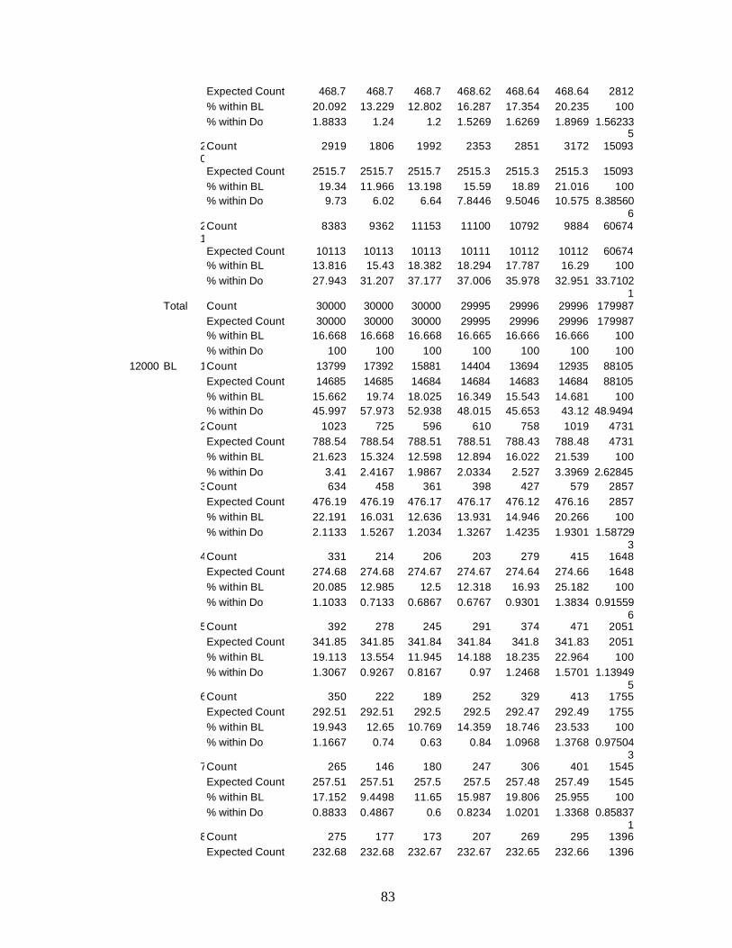
83
Expected Count 468.7 468.7 468.7 468.62 468.64 468.64 2812 % within BL 20.092 13.229 12.802 16.287 17.354 20.235 100 % within Do 1.8833 1.24 1.2 1.5269 1.6269 1.8969 1.56233
5 2
0Count 2919 1806 1992 2353 2851 3172 15093
Expected Count 2515.7 2515.7 2515.7 2515.3 2515.3 2515.3 15093 % within BL 19.34 11.966 13.198 15.59 18.89 21.016 100 % within Do 9.73 6.02 6.64 7.8446 9.5046 10.575 8.38560
6 2
1Count 8383 9362 11153 11100 10792 9884 60674
Expected Count 10113 10113 10113 10111 10112 10112 60674 % within BL 13.816 15.43 18.382 18.294 17.787 16.29 100 % within Do 27.943 31.207 37.177 37.006 35.978 32.951 33.7102
1 Total Count 30000 30000 30000 29995 29996 29996 179987 Expected Count 30000 30000 30000 29995 29996 29996 179987 % within BL 16.668 16.668 16.668 16.665 16.666 16.666 100 % within Do 100 100 100 100 100 100 100
12000 BL 1Count 13799 17392 15881 14404 13694 12935 88105 Expected Count 14685 14685 14684 14684 14683 14684 88105 % within BL 15.662 19.74 18.025 16.349 15.543 14.681 100 % within Do 45.997 57.973 52.938 48.015 45.653 43.12 48.9494 2Count 1023 725 596 610 758 1019 4731 Expected Count 788.54 788.54 788.51 788.51 788.43 788.48 4731 % within BL 21.623 15.324 12.598 12.894 16.022 21.539 100 % within Do 3.41 2.4167 1.9867 2.0334 2.527 3.3969 2.62845 3Count 634 458 361 398 427 579 2857 Expected Count 476.19 476.19 476.17 476.17 476.12 476.16 2857 % within BL 22.191 16.031 12.636 13.931 14.946 20.266 100 % within Do 2.1133 1.5267 1.2034 1.3267 1.4235 1.9301 1.58729
3 4Count 331 214 206 203 279 415 1648 Expected Count 274.68 274.68 274.67 274.67 274.64 274.66 1648 % within BL 20.085 12.985 12.5 12.318 16.93 25.182 100 % within Do 1.1033 0.7133 0.6867 0.6767 0.9301 1.3834 0.91559
6 5Count 392 278 245 291 374 471 2051 Expected Count 341.85 341.85 341.84 341.84 341.8 341.83 2051 % within BL 19.113 13.554 11.945 14.188 18.235 22.964 100 % within Do 1.3067 0.9267 0.8167 0.97 1.2468 1.5701 1.13949
5 6Count 350 222 189 252 329 413 1755 Expected Count 292.51 292.51 292.5 292.5 292.47 292.49 1755 % within BL 19.943 12.65 10.769 14.359 18.746 23.533 100 % within Do 1.1667 0.74 0.63 0.84 1.0968 1.3768 0.97504
3 7Count 265 146 180 247 306 401 1545 Expected Count 257.51 257.51 257.5 257.5 257.48 257.49 1545 % within BL 17.152 9.4498 11.65 15.987 19.806 25.955 100 % within Do 0.8833 0.4867 0.6 0.8234 1.0201 1.3368 0.85837
1 8Count 275 177 173 207 269 295 1396 Expected Count 232.68 232.68 232.67 232.67 232.65 232.66 1396

84
% within BL 19.699 12.679 12.393 14.828 19.269 21.132 100 % within Do 0.9167 0.59 0.5767 0.69 0.8968 0.9834 0.77559 9Count 214 132 142 185 222 262 1157 Expected Count 192.84 192.84 192.84 192.84 192.82 192.83 1157 % within BL 18.496 11.409 12.273 15.99 19.188 22.645 100 % within Do 0.7133 0.44 0.4733 0.6167 0.7401 0.8734 0.64280
6 1
0Count 294 183 207 246 277 355 1562
Expected Count 260.34 260.34 260.34 260.34 260.31 260.33 1562 % within BL 18.822 11.716 13.252 15.749 17.734 22.727 100 % within Do 0.98 0.61 0.69 0.82 0.9235 1.1834 0.86781
6 1
1Count 256 193 174 204 242 328 1397
Expected Count 232.84 232.84 232.84 232.84 232.81 232.83 1397 % within BL 18.325 13.815 12.455 14.603 17.323 23.479 100 % within Do 0.8533 0.6433 0.58 0.68 0.8068 1.0934 0.77614
6 1
2Count 246 137 133 182 278 288 1264
Expected Count 210.68 210.68 210.67 210.67 210.65 210.66 1264 % within BL 19.462 10.839 10.522 14.399 21.994 22.785 100 % within Do 0.82 0.4567 0.4433 0.6067 0.9268 0.9601 0.70225
3 1
3Count 189 131 140 205 250 285 1200
Expected Count 200.01 200.01 200 200 199.98 200 1200 % within BL 15.75 10.917 11.667 17.083 20.833 23.75 100 % within Do 0.63 0.4367 0.4667 0.6834 0.8334 0.9501 0.66669
6 1
4Count 225 142 129 187 229 262 1174
Expected Count 195.68 195.68 195.67 195.67 195.65 195.66 1174 % within BL 19.165 12.095 10.988 15.928 19.506 22.317 100 % within Do 0.75 0.4733 0.43 0.6234 0.7634 0.8734 0.65225
1 1
5Count 223 187 192 226 228 234 1290
Expected Count 215.01 215.01 215 215 214.98 215 1290 % within BL 17.287 14.496 14.884 17.519 17.674 18.14 100 % within Do 0.7433 0.6233 0.64 0.7534 0.7601 0.7801 0.71669
9 1
6Count 211 129 132 143 199 247 1061
Expected Count 176.84 176.84 176.84 176.84 176.82 176.83 1061 % within BL 19.887 12.158 12.441 13.478 18.756 23.28 100 % within Do 0.7033 0.43 0.44 0.4767 0.6634 0.8234 0.58947
1 1
7Count 213 146 157 187 243 249 1195
Expected Count 199.18 199.18 199.17 199.17 199.15 199.16 1195 % within BL 17.824 12.218 13.138 15.649 20.335 20.837 100 % within Do 0.71 0.4867 0.5234 0.6234 0.8101 0.8301 0.66391
8 1
8Count 288 178 198 243 274 315 1496

85
Expected Count 249.34 249.34 249.34 249.34 249.31 249.33 1496 % within BL 19.251 11.898 13.235 16.243 18.316 21.056 100 % within Do 0.96 0.5933 0.66 0.81 0.9135 1.0501 0.83114
8 1
9Count 580 379 356 408 416 475 2614
Expected Count 435.69 435.69 435.67 435.67 435.63 435.66 2614 % within BL 22.188 14.499 13.619 15.608 15.914 18.171 100 % within Do 1.9333 1.2633 1.1867 1.36 1.3869 1.5834 1.45228
7 2
0Count 2898 1688 1746 1952 2278 2459 13021
Expected Count 2170.3 2170.3 2170.2 2170.2 2170 2170.1 13021 % within BL 22.256 12.964 13.409 14.991 17.495 18.885 100 % within Do 9.66 5.6267 5.8202 6.5069 7.5943 8.1972 7.23421 2
1Count 7094 6763 8462 9019 8424 7711 47473
Expected Count 7912.5 7912.5 7912.3 7912.3 7911.5 7912 47473 % within BL 14.943 14.246 17.825 18.998 17.745 16.243 100 % within Do 23.647 22.543 28.208 30.064 28.084 25.705 26.3750
6 Total Count 30000 30000 29999 29999 29996 29998 179992 Expected Count 30000 30000 29999 29999 29996 29998 179992 % within BL 16.667 16.667 16.667 16.667 16.665 16.666 100 % within Do 100 100 100 100 100 100 100
14000 BL 1Count 14429 18980 18598 16751 15760 14086 98604 Expected Count 16620 16620 16619 16617 16618 15509 98604 % within BL 14.633 19.249 18.861 16.988 15.983 14.285 100 % within Do 48.097 63.267 62 55.846 52.54 50.316 55.4008 2Count 1088 791 641 625 686 860 4691 Expected Count 790.69 790.69 790.61 790.56 790.59 737.85 4691 % within BL 23.193 16.862 13.664 13.323 14.624 18.333 100 % within Do 3.6267 2.6367 2.1369 2.0837 2.287 3.072 2.63564
5 3Count 663 490 377 399 414 452 2795 Expected Count 471.11 471.11 471.07 471.03 471.05 439.63 2795 % within BL 23.721 17.531 13.488 14.275 14.812 16.172 100 % within Do 2.21 1.6333 1.2568 1.3302 1.3802 1.6146 1.57037
5 4Count 349 207 204 194 267 339 1560 Expected Count 262.95 262.95 262.92 262.9 262.91 245.37 1560 % within BL 22.372 13.269 13.077 12.436 17.115 21.731 100 % within Do 1.1633 0.69 0.6801 0.6468 0.8901 1.2109 0.87648
8 5Count 424 293 266 280 361 385 2009 Expected Count 338.63 338.63 338.59 338.57 338.58 316 2009 % within BL 21.105 14.584 13.24 13.937 17.969 19.164 100 % within Do 1.4133 0.9767 0.8868 0.9335 1.2035 1.3752 1.12875
9 6Count 366 230 183 243 290 333 1645 Expected Count 277.27 277.27 277.25 277.23 277.24 258.74 1645 % within BL 22.249 13.982 11.125 14.772 17.629 20.243 100 % within Do 1.22 0.7667 0.6101 0.8101 0.9668 1.1895 0.92424
6 7Count 278 161 180 242 282 330 1473

86
Expected Count 248.28 248.28 248.26 248.24 248.25 231.69 1473 % within BL 18.873 10.93 12.22 16.429 19.145 22.403 100 % within Do 0.9267 0.5367 0.6001 0.8068 0.9401 1.1788 0.82760
7 8Count 301 212 161 197 242 252 1365 Expected Count 230.08 230.08 230.06 230.04 230.05 214.7 1365 % within BL 22.051 15.531 11.795 14.432 17.729 18.462 100 % within Do 1.0033 0.7067 0.5367 0.6568 0.8068 0.9002 0.76692
7 9Count 226 125 140 174 206 217 1088 Expected Count 183.39 183.39 183.37 183.36 183.36 171.13 1088 % within BL 20.772 11.489 12.868 15.993 18.934 19.945 100 % within Do 0.7533 0.4167 0.4667 0.5801 0.6868 0.7751 0.61129
4 1
0Count 315 208 195 240 264 295 1517
Expected Count 255.7 255.7 255.67 255.66 255.66 238.61 1517 % within BL 20.765 13.711 12.854 15.821 17.403 19.446 100 % within Do 1.05 0.6933 0.6501 0.8001 0.8801 1.0538 0.85232
9 1
1Count 271 197 169 202 224 259 1322
Expected Count 222.83 222.83 222.81 222.79 222.8 207.94 1322 % within BL 20.499 14.902 12.784 15.28 16.944 19.592 100 % within Do 0.9033 0.6567 0.5634 0.6734 0.7468 0.9252 0.74276
8 1
2Count 254 135 134 159 237 233 1152
Expected Count 194.18 194.18 194.16 194.14 194.15 181.2 1152 % within BL 22.049 11.719 11.632 13.802 20.573 20.226 100 % within Do 0.8467 0.45 0.4467 0.5301 0.7901 0.8323 0.64725
3 1
3Count 195 141 133 185 233 230 1117
Expected Count 188.28 188.28 188.26 188.25 188.25 175.69 1117 % within BL 17.457 12.623 11.907 16.562 20.859 20.591 100 % within Do 0.65 0.47 0.4434 0.6168 0.7768 0.8216 0.62758
8 1
4Count 232 146 125 167 199 217 1086
Expected Count 183.05 183.05 183.03 183.02 183.03 170.82 1086 % within BL 21.363 13.444 11.51 15.378 18.324 19.982 100 % within Do 0.7733 0.4867 0.4167 0.5568 0.6634 0.7751 0.61017
1 1
5Count 228 186 185 217 206 200 1222
Expected Count 205.97 205.97 205.95 205.94 205.95 192.21 1222 % within BL 18.658 15.221 15.139 17.758 16.858 16.367 100 % within Do 0.76 0.62 0.6167 0.7235 0.6868 0.7144 0.68658
2 1
6Count 216 118 123 133 167 201 958
Expected Count 161.48 161.48 161.46 161.45 161.45 150.68 958 % within BL 22.547 12.317 12.839 13.883 17.432 20.981 100 % within Do 0.72 0.3933 0.41 0.4434 0.5567 0.718 0.53825
4 1Count 218 142 159 177 206 195 1097

87
7 Expected Count 184.91 184.91 184.89 184.87 184.88 172.55 1097 % within BL 19.872 12.944 14.494 16.135 18.778 17.776 100 % within Do 0.7267 0.4733 0.5301 0.5901 0.6868 0.6966 0.61635
1 1
8Count 291 180 188 240 254 260 1413
Expected Count 238.17 238.17 238.14 238.13 238.14 222.25 1413 % within BL 20.594 12.739 13.305 16.985 17.976 18.401 100 % within Do 0.97 0.6 0.6267 0.8001 0.8468 0.9287 0.79389
6 1
9Count 590 375 349 382 377 382 2455
Expected Count 413.8 413.8 413.76 413.73 413.75 386.15 2455 % within BL 24.033 15.275 14.216 15.56 15.356 15.56 100 % within Do 1.9667 1.25 1.1634 1.2735 1.2568 1.3645 1.37934
5 2
0Count 2869 1568 1538 1657 1957 1969 11558
Expected Count 1948.2 1948.2 1948 1947.8 1947.9 1818 11558 % within BL 24.823 13.566 13.307 14.336 16.932 17.036 100 % within Do 9.5633 5.2267 5.1272 5.5243 6.5242 7.0334 6.49387
9 2
1Count 6197 5115 5949 7131 7164 6300 37856
Expected Count 6380.8 6380.8 6380.2 6379.8 6380 5954.4 37856 % within BL 16.37 13.512 15.715 18.837 18.924 16.642 100 % within Do 20.657 17.05 19.832 23.774 23.883 22.504 21.2694
5 Total Count 30000 30000 29997 29995 29996 27995 177983 Expected Count 30000 30000 29997 29995 29996 27995 177983 % within BL 16.856 16.856 16.854 16.853 16.853 15.729 100 % within Do 100 100 100 100 100 100 100
Top Related