


Languages
Pages
Legal


Neutrino Factory Feasibility Study-IINeutrino Factory Feasibility Study-II
Editors Meeting January 29-312001at BNL
Editors Meeting January 29-312001at BNL

Elevation
Plan
Ring Layout
Study-II Challenge: Storage Ring Footprint
For Study-II it is important tofind a solution that gives avery compact arc.*
*Here arc definition includes all regions with dipoles.
B. Parker 29-Jan-01
• For given straight section decay ratio a shorter arc reduces the site footprint.
• For given straight section length a shorter arc increases ν production efficiency.


C =1753 m
Storage Ring Footprint: Ring Scaling Part 1First consider energy scaling from 50 to 20 GeV
B. Parker 29-Jan-01
C = 700 m
C = 840 m
C = 530 m
Overly naive scaling gives:1753 m x (2/5) ≈ 700 m
• 250% larger emittance at 20 GeV drives larger magnet apertures (longer ends, weaker fields).
• The magnet ends do not follow above scaling.
• So want to have shorter cell lengths to reduce arc beta and dispersion maxima.
More involved scaling yields20 GeV circumference > 840 m. Yet our design has 530 m.

Storage Ring Footprint: Ring Scaling Part 2But in practice we see that most of the reductioncomes from having fewer cells. We expect to haveonly a small reduction in cell length (example 15%).
B. Parker 29-Jan-01
Study-I Cell: separated function, 90° phase advance and 9.8 m length.
1 m 2.4 m, B = 6 T 1 m 2.4 m, B = 6 T
Q, SX Q, SXDDD D
0.75 m 0.75 m 0.75 m 0.75 m
1'st Try: separated function, 90° phase advance and 8.4 m length.
0.825 m 1.875 m, B = 7 T 0.825 m 1.875 m, B = 7 T
Q, SX Q, SXDDD D
0.75 m 0.75 m 0.75 m 0.75 m
2'nd Try: separated function, 90° phase advance and 8.4 m length.
Q, SX Q, SXD D
0.52 m 2.18 m, B = 6 T 0.52 m 2.18 m, B = 6 T0.75 m 0.75 m 0.75 m 0.75 m
Max. beta ≈ 16 m & Max. Dispersion ≈ 1.1 m (50 Gev, 173 mr/cell)
Max. beta ≈ 14 m & Max. Dispersion ≈ 2.2 m (20 Gev, 393 mr/cell)
Max. beta ≈ 14 m & Max. Dispersion ≈ 2.2 m (20 Gev, 393 mr/cell)
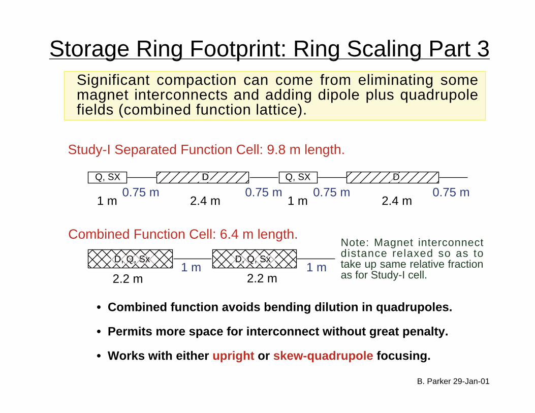
Storage Ring Footprint: Ring Scaling Part 3Significant compaction can come from eliminating somemagnet interconnects and adding dipole plus quadrupolefields (combined function lattice).
B. Parker 29-Jan-01
Study-I Separated Function Cell: 9.8 m length.
1 m 2.4 m 1 m 2.4 m
Q, SX Q, SXDDD D
0.75 m 0.75 m 0.75 m 0.75 m
Combined Function Cell: 6.4 m length.
2.2 m
D, Q, Sx1 m
2.2 m1 m
D, Q, Sx
Note: Magnet interconnectdistance relaxed so as totake up same relative fractionas for Study-I cell.
• Combined function avoids bending dilution in quadrupoles.
• Permits more space for interconnect without great penalty.
• Works with either upright or skew-quadrupole focusing.
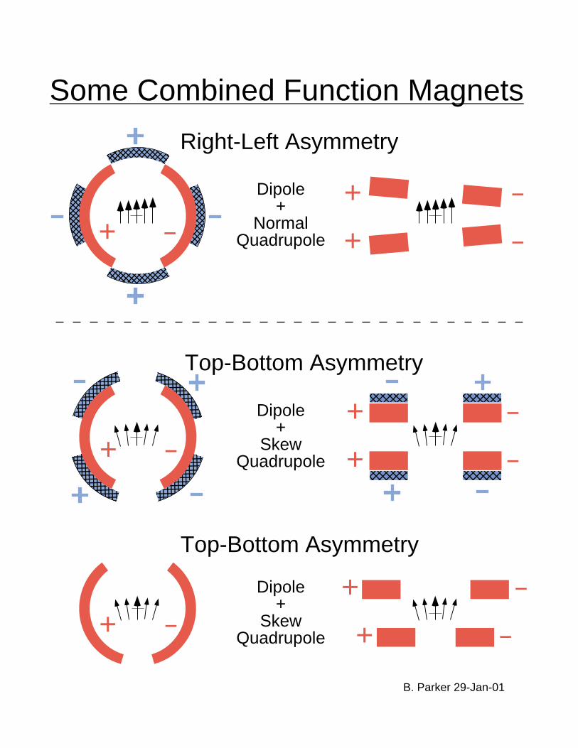
Some Combined Function Magnets
B. Parker 29-Jan-01
Dipole+
NormalQuadrupole
Dipole+
SkewQuadrupole
Dipole+
SkewQuadrupole
+ -
+ -
+ -
+ -
+ -
+ -
+ -
+ -
+ -
Right-Left Asymmetry
Top-Bottom Asymmetry
Top-Bottom Asymmetry

Warm Yoke
Ring Center
Flat Coil (Superconducter Nb3Sn)
Original Storage Ring Dipole Concept
Shield
But a separated function cell witha warm quadrupole uses up space.
B. Parker 29-Jan-01
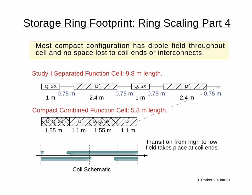
Storage Ring Footprint: Ring Scaling Part 4
Most compact configuration has dipole field throughoutcell and no space lost to coil ends or interconnects.
B. Parker 29-Jan-01
Study-I Separated Function Cell: 9.8 m length.
1 m 2.4 m 1 m
Q, SX Q, SXDDD D
0.75 m 0.75 m 0.75 m
1.55 m
D, Q, Sx
1.1 m 1.55 m 1.1 m
D, Q, Sx DDD DDD
Coil Schematic
Transition from high to lowfield takes place at coil ends.
Compact Combined Function Cell: 5.3 m length.
2.4 m0.75 m

Combined Function Skew Quadrupole Cell Principle
File set: mu_mf09b, 29-Jan-01, B. Parker
Plan View
Elevation View
Full coil overlapgives the full field,B = 7 T, but G=0
Single coil for half field,B = 3.5T, but G=20T/m
A
A
B
B
Section A-A
Section B-B
B = 7 TG = 0 T/mNo skew
B = 3.5 TG = 20 T/mSkew Quad
• Flat coils are longitudinally staggered in a warm iron yoke.• Coil ends are spread longitudinally to adjust integral harmonics.• Coils bend in the horizontal plane to follow circulating beam.
Net result is to use space which isnormally wasted between coil ends.
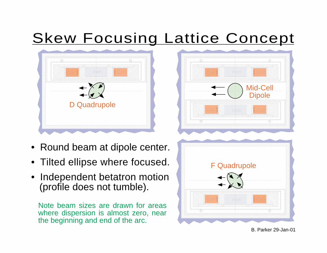
D Quadrupole
F Quadrupole
Mid-CellDipole
Skew Focusing Lattice Concept
B. Parker 29-Jan-01
Note beam sizes are drawn for areaswhere dispersion is almost zero, nearthe beginning and end of the arc.
• Round beam at dipole center.
• Tilted ellipse where focused.
• Independent betatron motion (profile does not tumble).

Skew Quadrupole Lattice Design Principles
File set: mu_mf09a, 18-Dec-00, B. Parker
≡Skew Quadrupole Lattice Fully Coupled Lattice
The lattices presented here are uncoupled. Theyare special only in that the betatron eigenplanes(denoted A,B) line up with ±45° rather than thehorizontal (X) and vertical (Y) axes.
AB
X
YUseful Trick:
Every dipole with bend radius, ρ, hasa weak normal focusing component,k = -1/(2ρ2) added in order to makethe focusing cylindrically symmetric.

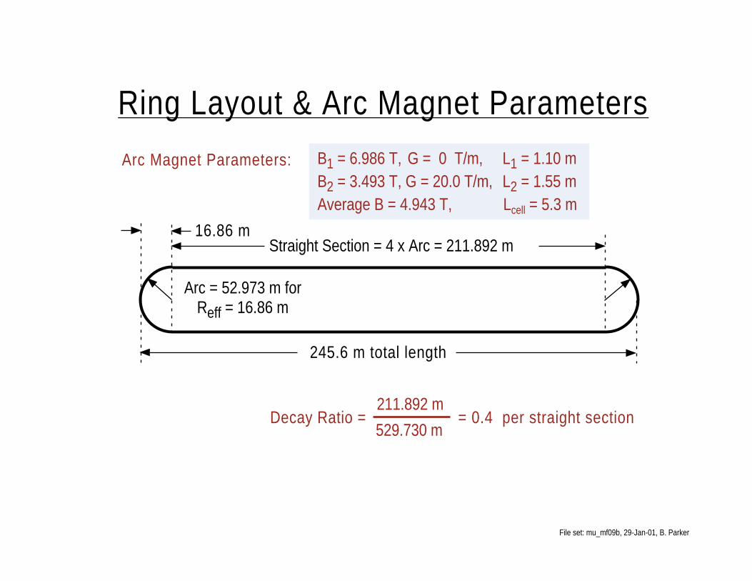
Straight Section = 4 x Arc = 211.892 m
Arc = 52.973 m forReff = 16.86 m
16.86 m
245.6 m total length
Decay Ratio =211.892 m
= 0.4 per straight section529.730 m
Ring Layout & Arc Magnet Parameters
B1 = 6.986 T, G = 0 T/m, L1 = 1.10 mB2 = 3.493 T, G = 20.0 T/m, L2 = 1.55 mAverage B = 4.943 T, Lcell = 5.3 m
Arc Magnet Parameters:
File set: mu_mf09b, 29-Jan-01, B. Parker

Storage Ring Lattice Modules and Their Functions
File set: mu_mf09b, 29-Jan-01, B. Parker
Arcs have 10 cellsBeta peak = 8.8 mPhase/cell = 60°Cells w/o bending near ends for dispersion suppressionSkew-sextupoles are used in 6 central cells for chromaticity correction
Production straight is 4 times longer than arc for a 0.4decay length ratio. Average beta of 91 m adds 1% to theν-beam divergence. Will introduce normal quadrupolesfor coupling control. Also use long drift regions for RF?
Second straight has natural betaabout double that in arcs but cells areadjusted to make a phase tromboneyield ing 1 uni t phase di f ferencebetween A and B eigenplanes. Ringtune adjustment is done here. Alsocan introduce injection elements here.
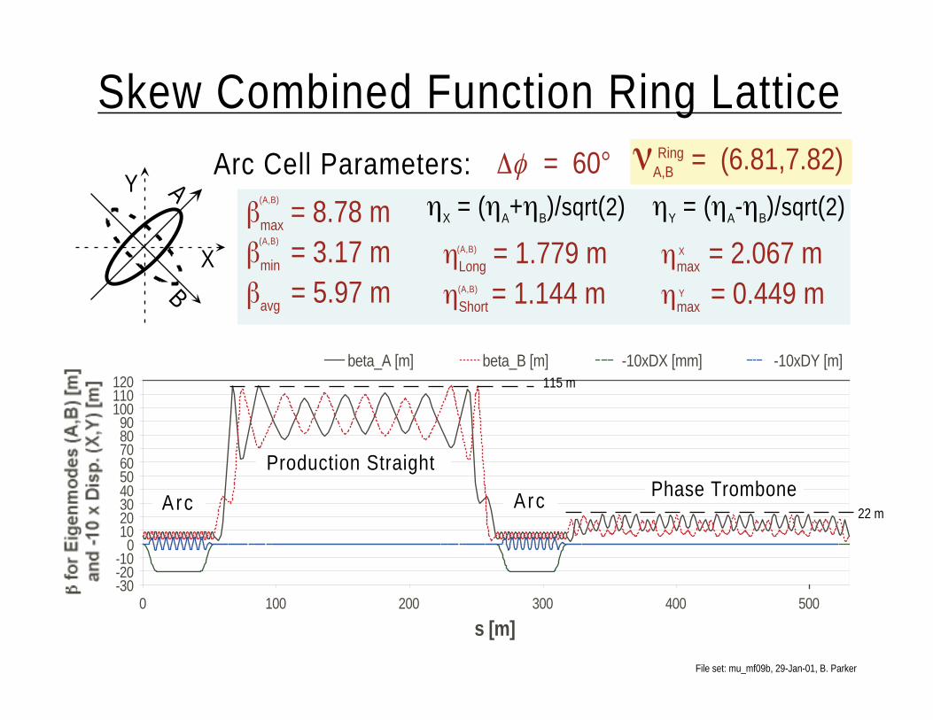
νA,B = (6.81,7.82)
-30-20-10
0102030405060708090
100110120
0 100 200 300 400 500
s [m]
beta_A [m] beta_B [m] -10xDX [mm] -10xDY [m]
βmax = 8.78 mβmin = 3.17 mβavg = 5.97 m
(A,B)
(A,B)
AB
X
Y
Skew Combined Function Ring Lattice
ηLong = 1.779 mηShort = 1.144 m
(A,B)
(A,B)
ηmax = 2.067 mηmax = 0.449 m
X
Y
Arc Cell Parameters:ηX = (ηA+ηB)/sqrt(2) ηY = (ηA-ηB)/sqrt(2)
Arc
Production Straight
Arc Phase Trombone
File set: mu_mf09b, 29-Jan-01, B. Parker
∆φ = 60°
115 m
22 m
Ring
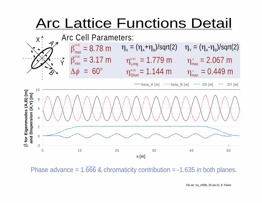
βmax = 8.78 mβmin = 3.17 m∆φ = 60°
(A,B)
(A,B)
AB
X
Y
Arc Lattice Functions Detail
ηLong = 1.779 mηShort = 1.144 m
(A,B)
(A,B)
ηmax = 2.067 mηmax = 0.449 m
X
Y
Arc Cell Parameters:ηX = (ηA+ηB)/sqrt(2) ηY = (ηA-ηB)/sqrt(2)
Phase advance = 1.666 & chromaticity contribution = -1.635 in both planes.
File set: mu_mf09b, 29-Jan-01, B. Parker
-2
0
2
4
6
8
10
0 10 20 30 40 50
s [m]
beta_A [m] beta_B [m] DX [m] DY [m]
β f
or
Eig
en
mo
des (
A,B
) [m
]an
d D
isp
ers
ion
(X
,Y)
[m]

Arc Lattice Dispersion Suppression Scheme
File set: mu_mf09b, 29-Jan-01, B. Parker
Cell #1
Cell #2
Cell #3
Cell #4
Cell #5
Cell #6
Cell #7
Cell #8
Cell #9
Cell #10
No Bends No Bends
With 60° phase advance*, the central six cells make up an achromat.Peak dispersion is reduced via two additional cells at each arc endwhere one of the cells has zero dipole bending.
Focusing is different in no bend cells and this leads to a small mis-match which is fixed by adjusting cell length and quadrupole strength.Could also match by only adjusting strengths in outer cells (1-2,9-10).
*Note for 90° phase advance the outer cells (1-2,9-10) should have 1/2 dipole bending.

Skew Sextupole Chromaticity Correction Schemes
File set: mu_mf09b, 29-Jan-01, B. Parker
For the skew quadrupole lattices considered here, we find it much better to useskew sextupoles than normal sextupoles for chromaticity correction as theneeded strengths are at least a factor 4.5 lower!
With a phase advance per cell of 60° it is possible to make a chromaticity correc-tion scheme using the central six cells (3-8) very similar to the original HERAecorrection scheme which is very flexible and exhibits good dynamic aperture.
Cell #1
Cell #2
Cell #3
Cell #4
Cell #5
Cell #6
Cell #7
Cell #8
Cell #9
Cell #10
D DE EA AB BC C
Note with three skew sextupole families it should be possible to make completechromatic correction at an arbitrary location in the ring (e.g. injection kicker).

Skew Sextupole Chromaticity Correction Schemes
File set: mu_mf09b, 29-Jan-01, B. Parker
For central 6 skew sextupoles both first order and higher order moments cancel!
12
36
54
A
C BA
CB 78
910
D
D
E
E
Diagramφ Phase Advance = 60°
3,64,7
5,8
A
B
C
2
9
1,10D
D
E
E
Diagram2 φ Phase Advance = 120°
While using all 10 locations reduces strengths needed for linear chromaticitycorrection, such an arrangement would likely drive higher order resonances.
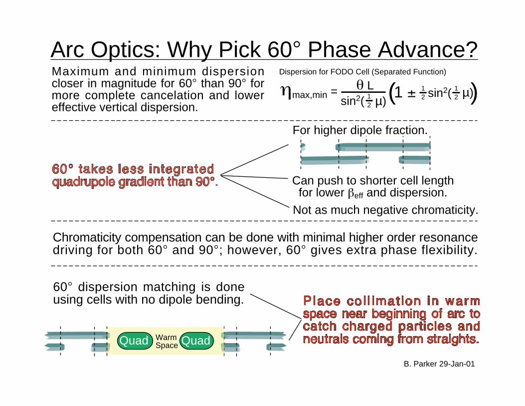
Arc Optics: Why Pick 60° Phase Advance?Maximum and minimum dispersioncloser in magnitude for 60° than 90° formore complete cancelation and lowereffective vertical dispersion.
B. Parker 29-Jan-01
Not as much negative chromaticity.
ηmax,min = θ Lsin2( 1
2 µ)( )1 ± sin2( 12 µ)1
2
Dispersion for FODO Cell (Separated Function)
60° dispersion matching is doneusing cells with no dipole bending.
For higher dipole fraction.
Can push to shorter cell lengthfor lower βeff and dispersion.
Chromaticity compensation can be done with minimal higher order resonancedriving for both 60° and 90°; however, 60° gives extra phase flexibility.
Quad QuadWarmSpace

What does the dipole magnet cross sectionlook like for the toy model study?
X (cm)
SuperconductorWarm beam pipe
PhotonsDecay electrons
Warm yoke
Ring Center

What are the magnets like?

Magnet Cross Section Schematic: Double Coil
B. Parker 29-Jan-01
Decay Electrons
43π mm Norm. Acceptance
∆p/p = ±2.2% for µ74 mm
Yoke
Ring Center
OuterVacuumJacket
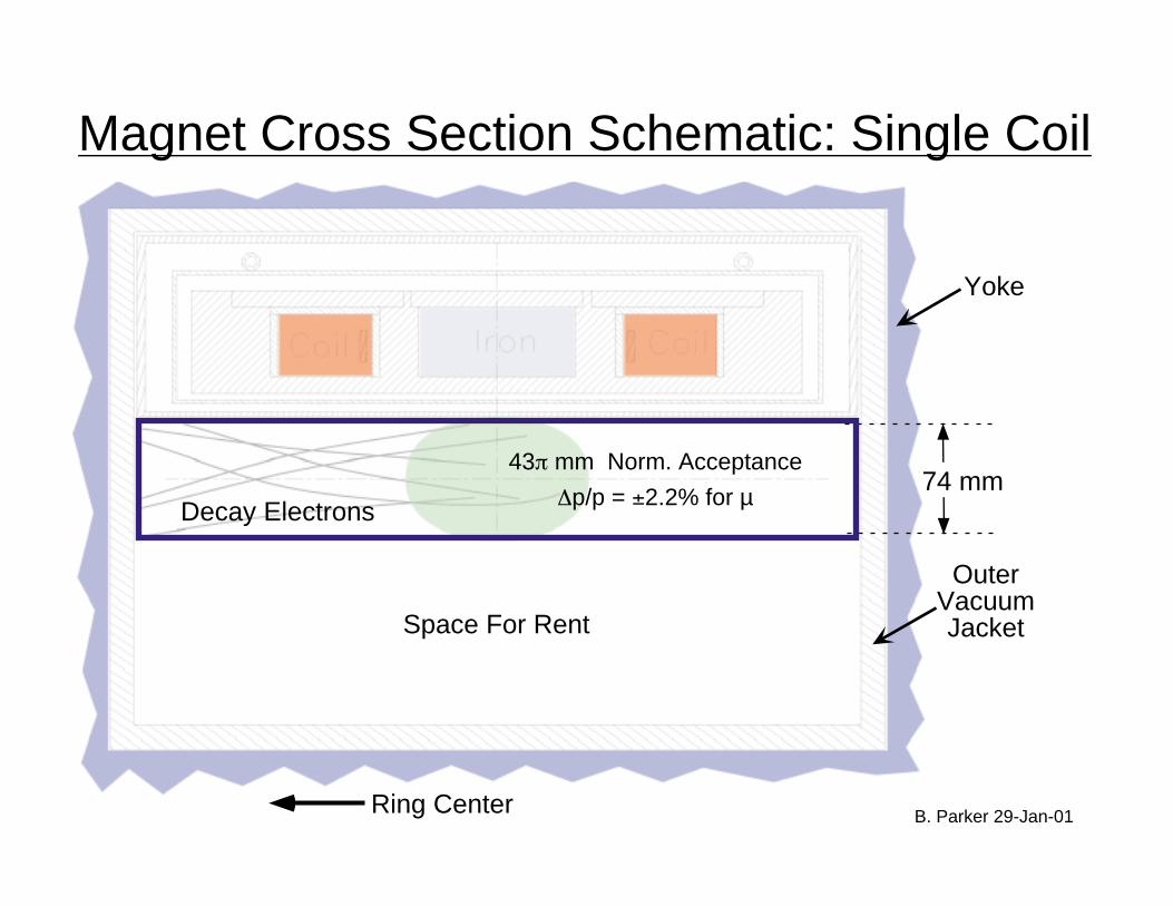
Magnet Cross Section Schematic: Single Coil
B. Parker 29-Jan-01
Decay Electrons
43π mm Norm. Acceptance
∆p/p = ±2.2% for µ74 mm
Yoke
Ring Center
OuterVacuumJacketSpace For Rent
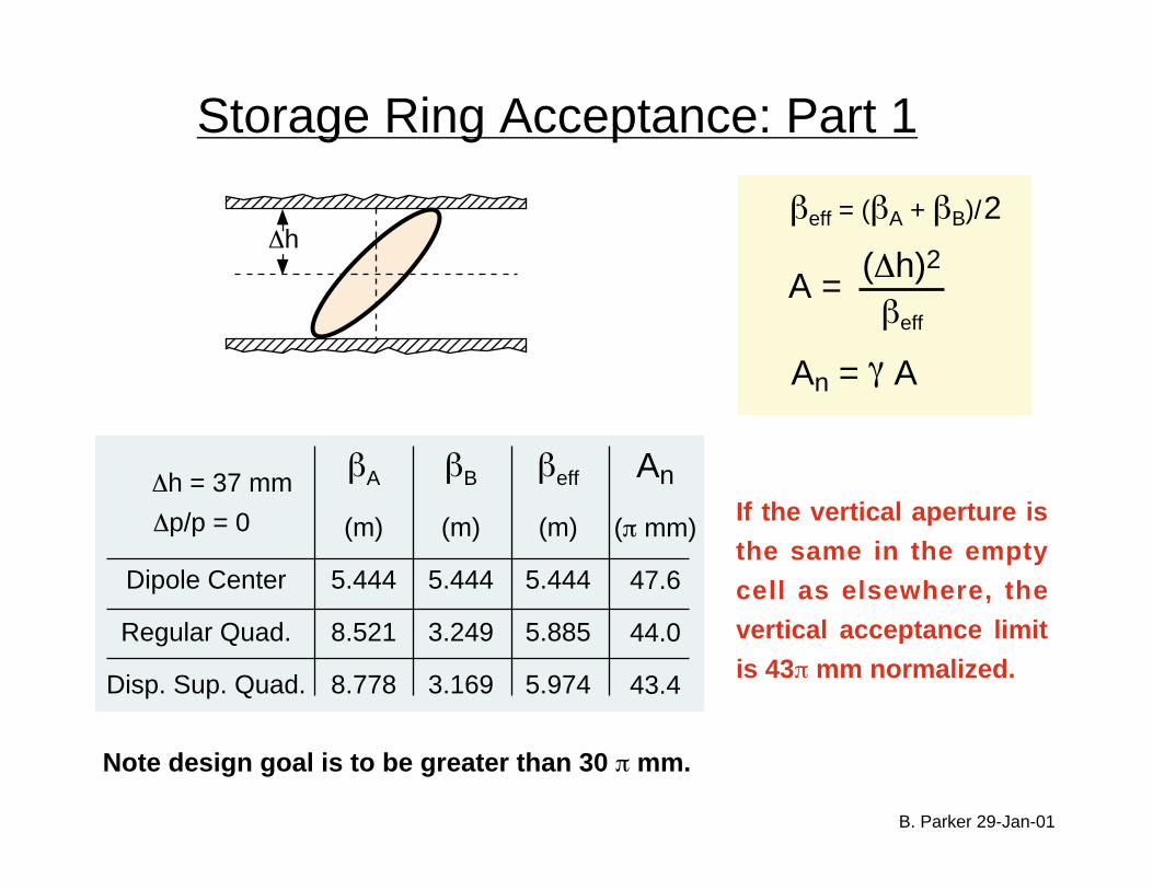
Storage Ring Acceptance: Part 1
B. Parker 29-Jan-01
Note design goal is to be greater than 30 π mm.
∆hβeff = (βA + βB)/2
A = (∆h)2
βeff
An = γ A
∆h = 37 mm
Dipole Center
Regular Quad.
Disp. Sup. Quad.
βA
(m)
5.444
8.521
8.778
βB
(m)
5.444
3.249
3.169
βeff
(m)
5.444
5.885
5.974
An
(π mm)
47.6
44.0
43.4
∆p/p = 0 If the vertical aperture is
the same in the empty
cell as elsewhere, the
vertical acceptance limit
is 43π mm normalized.

Storage Ring Acceptance: Part 2
B. Parker 29-Jan-01
For large ∆p/p we find that β and η are changed from the linear optics.
Dipole Center
Regular Quad.
End Disp. Sup.
ηX
(m)
2.029
2.067
2.030
ηY
(m)
0
0.449
0.324
|∆X|
(mm)
45
45
45
|∆Y|
(mm)
0
10
7
For ∆p/p = -2.2% we find ∆X = -63 mm, ∆Y = -16 mm
∆x- ∆x+
(Linear Approx.)
∆X ≈ ηX x ∆p/p
∆Y ≈ ηY x ∆p/p
And the closed orbit does not move symmetrically for ±∆p/p.
For ∆p/p = +2.2% we find ∆X = 46 mm, ∆Y = 12 mm
Worst Case*:
(±54 mm)*With chromaticity correction turned on (even larger beta-beat if it is turned off).
Closed OrbitCalculation for∆p/p = ±2.2%

t
Storage Ring Acceptance: Part 3
B. Parker 29-Jan-01
• Straight section warm quadrupole parameters look plausible.
• By defining more magnet types (length, pole radius) could
optimize trade off between production and operating costs.
• Must consider constraints from other accelerator systems
(vacuum, rf, injection, tuning/abort and diagnostic).
• In some areas a non-circular beam pipe may be appropriate.
Production
Phase Trombone
βmax
(m)
115
22
rpole
(mm)
175
75
An
(π mm)
48
43
Use max(βA,βB) for circular aperture acceptance in the straights.
*Phase trombone quadrupoles with largest gradient have smallerβ so r and Bpole could be reduced; however providing full aperturefor injected beam, while it is off axis, may not allow this reduction.
ηA ηB = 0= r
(mm)
170
71
Bpole
(T)
0.62
0.93*
An = γ r2/βmax
Warm Skew Quadrupole Schematic

Special Considerations?
-30-20-10
0102030405060708090
100110120
0 100 200 300 400 500
s [m]
beta_A [m] beta_B [m] -10xDX [mm] -10xDY [m]
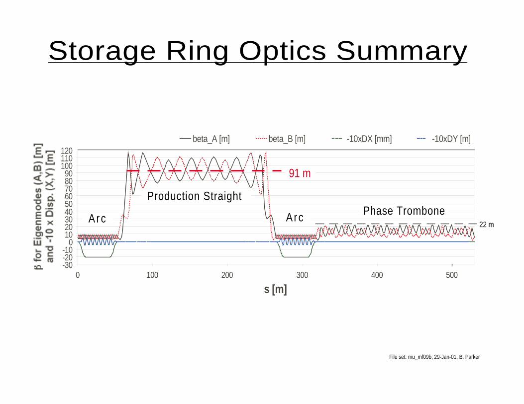
Arc
Production Straight
Arc Phase Trombone22 m
Storage Ring Optics Summary
File set: mu_mf09b, 29-Jan-01, B. Parker
91 m
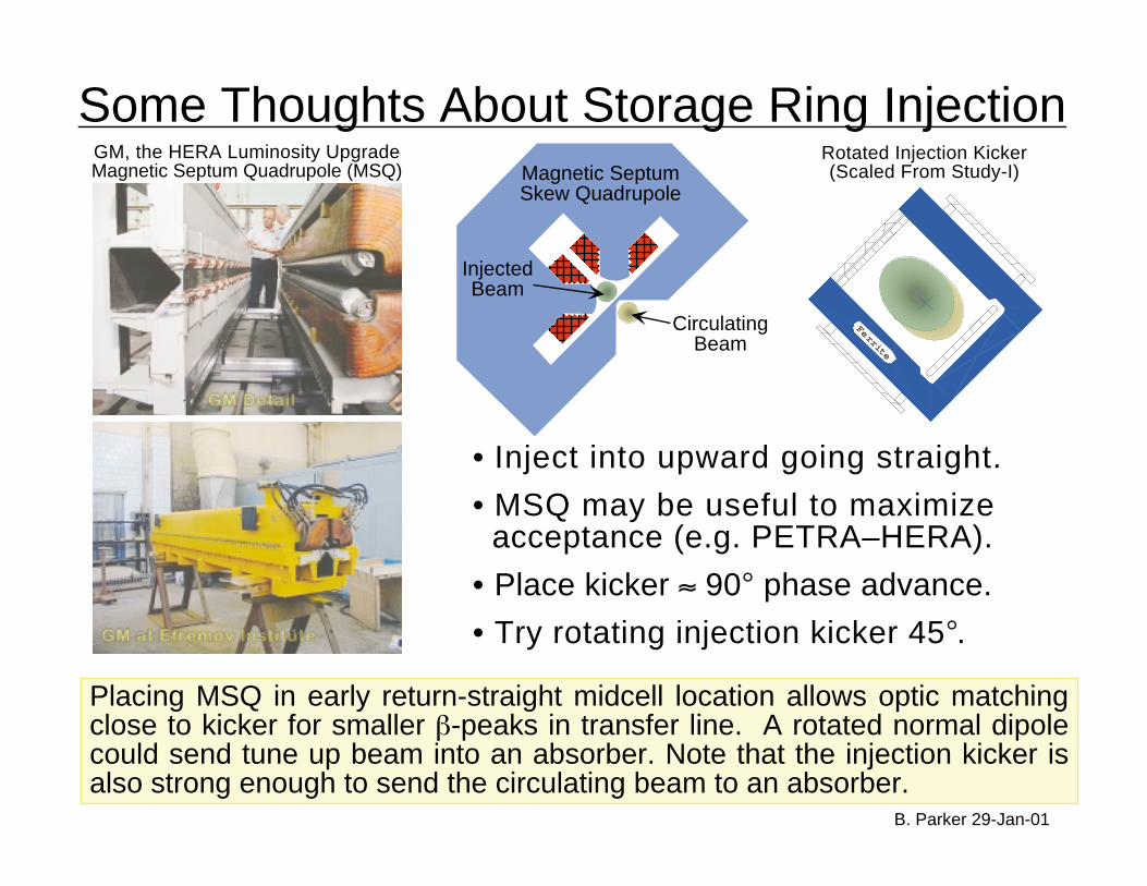
Some Thoughts About Storage Ring Injection
Placing MSQ in early return-straight midcell location allows optic matchingclose to kicker for smaller β-peaks in transfer line. A rotated normal dipolecould send tune up beam into an absorber. Note that the injection kicker isalso strong enough to send the circulating beam to an absorber.
B. Parker 29-Jan-01
GM, the HERA Luminosity UpgradeMagnetic Septum Quadrupole (MSQ) Magnetic Septum
Skew Quadrupole
InjectedBeam
CirculatingBeam
• Inject into upward going straight.
• MSQ may be useful to maximize acceptance (e.g. PETRA–HERA).
• Place kicker ≈ 90° phase advance.
• Try rotating injection kicker 45°.
Rotated Injection Kicker(Scaled From Study-I)
0 50 100 150 2000
5
10
15
20
25
0
1
2
3
4
5
S - SArc = Distance From End of Arc (m)
f, In
crea
se D
ue to
Opt
ics
(%)
µ Optics ∆θ
% Increase
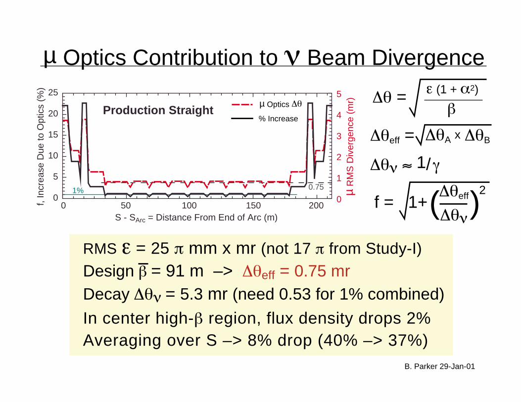
µ Optics Contribution to ν Beam Divergence
B. Parker 29-Jan-01
∆θ =
RMS ε = 25 π mm x mr (not 17 π from Study-I)
µ R
MS
Div
erge
nce
(mr)
0.751%
Production Straight
ε (1 + α2)
β
∆θeff = ∆θA ∆θBx
∆θν ≈ 1/ γ
f = 1+∆θeff
∆θν( )
2
Design β = 91 m –> ∆θeff = 0.75 mr Decay ∆θν = 5.3 mr (need 0.53 for 1% combined) In center high-β region, flux density drops 2% Averaging over S –> 8% drop (40% –> 37%)
B
B2
0
Dip
ole
Typ
e 1
Dip
ole
Typ
e 2
Dip
ole
Typ
e 1
Dip
ole
Typ
e 2
S
Hard Edge& Ideal
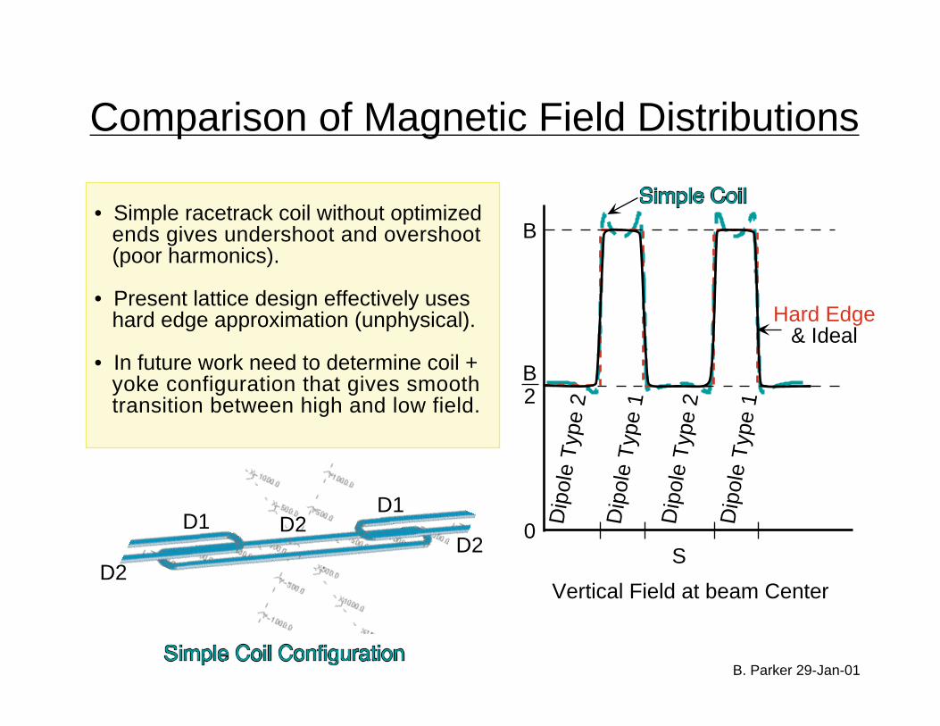
Comparison of Magnetic Field Distributions
• Simple racetrack coil without optimized ends gives undershoot and overshoot (poor harmonics).
• Present lattice design effectively uses hard edge approximation (unphysical).
• In future work need to determine coil + yoke configuration that gives smooth transition between high and low field.
B. Parker 29-Jan-01
Vertical Field at beam CenterD2
D1 D2D1
D2

+ -
+
-
+-
+
- +
-
+
-
+
-
+-
Skew Combined Function Optics Calculation
B. Parker 29-Jan-01
True Configuration Rotated By 45°
• Useful trick: rotate system 45° for upright eigenplanes - skew quadrupole –> normal quadrupole - dipole –> dipole rotated by 45° - skew sextupole –> sextupole rotated by 15°• Would like to avoid slicing by using a program which calculates correctly with combined fields (dipole + quadrupole + skew quadrupole + skew sextupole ...)

What are the magnets like?
Special Considerations?
Storage Ring and Magnet Design Summary
B. Parker 29-Jan-01
Top Related