Download - Neural Network and Time Series Analysis Approaches in ... · Electricity Consumption of Public Transportation Vehicles . ... cost and electrical network stability reasons. ... transfer

Neural Network and Time Series Analysis Approaches in Predicting

Electricity Consumption of Public Transportation Vehicles

CLAUDIO GUARNACCIA, JOSEPH QUARTIERI, CARMINE TEPEDINO

Department of Industrial Engineering

University of Salerno

Via Giovanni Paolo II 132, Fisciano (SA)

ITALY

[email protected] , [email protected] , [email protected]

SVETOSLAV ILIEV, SILVIYA POPOVA

Department of Bioengineering and Unique Instruments, Components and Structures

Institute of System Engineering and Robotics

Bulgarian Academy of Sciences

Sofia 1113, Akad. G. Bonchev str. bl 2

BULGARIA

[email protected] , [email protected]

Abstract: - Public transportation is a relevant issue to be considered in urban planning and in network design,

thus efficient management of modern electrical transport systems is a very important but difficult task. Tram

and trolley-bus transport in Sofia, Bulgaria, is largely developed. It is one of the largest consumers of electricity

in the city, which makes the question of electricity prediction very important for its operation. In fact, they are

required to notify the energy provider about the expected energy consumption for a given time range.

In this paper, two models are presented and compared in terms of predictive performances and error

distributions: one is based on Artificial Neural Networks (ANN) and the other on Time Series Analysis (TSA)

methods. They will be applied to the energy consumption related to public transportation, observed in Sofia,

during 2011, 2012 and 2013.

The main conclusion will be that the ANN model is much more precise but requires more preliminary

information and computational efforts, while the TSA model, against some errors, shows a low demanding

input entries and a lower power of calculation. In addition, the ANN model has a lower time range of

prediction, since it needs many recent inputs in order to produce the output. On the contrary, the TSA model

prediction, once the model has been calibrated on a certain time range, can be extended at any time period.

Key-Words: - Neural Network, Time Series Analysis, Electricity consumption prediction, Public transportation

1 Introduction In many big European cities, a large amount of

resources is adopted to develop an efficient network

of public transportation. The growing number of

inhabitants in urban areas leads to the necessity to

control the vehicular traffic due to private

transportation. For this reason, electrical tram and

trolley bus are preferred. The reduction of

combustion engines usage allows to reduce physical

and chemical polluting agents in highly populated

areas. Electrical engines are also very quiet, from

the acoustical point of view, and contribute to a

reduction of noise due to vehicular road traffic [1-

13].

Sofia, the capital of Bulgaria, has a very

developed network of electrical public

transportation vehicles. Anyway, the high electricity

absorption must be carefully monitored, both for

cost and electrical network stability reasons.

Different predictive models can be found in

literature, based on various approaches, such as

Neural Networks, Support Vector Machines, Fuzzy

logic, statistical tools, etc. [14-20].

In this paper, the predictive performances of two

different modelling techniques are compared. The

first method is based on an Artificial Neural

Network (ANN) of the multilayer perceptron

typology, thus able to extract the non-linear

relations in a data matrix. The second technique

makes statistical inference using the time periodicity

of the electrical absorption, by means of a model

based on Time Series Analysis (TSA).

WSEAS TRANSACTIONS on ENVIRONMENT and DEVELOPMENTClaudio Guarnaccia, Joseph Quartieri,

Carmine Tepedino, Svetoslav Iliev, Silviya Popova

E-ISSN: 2224-3496 312 Volume 11, 2015

mailto:[email protected]





After having presented the models, they will be

tested on 4 different datasets, that are four months of

2013. The differences between results obtained with

the two models will be highlighted in terms of error

evaluation and analysis.

The ANN model ensures a more accurate mean

prediction, but it needs more input information,

higher elaboration and computation abilities and

input data measured closer to the periods that are

under prediction. The TSA model is slightly less

precise in the prediction but needs as input only the

energy consumption registered in a sufficient

number of previous time periods. In addition, the

TSA model requires a low computing power and it

is able to provide reliable predictions even in time

periods far from the data used in the calibration and

in the parameters evaluation.

2 Models Presentation In this section, the ANN and TSA models will be

shortly presented and discussed.

The dataset is related to energy consumption in

2011, 2012 and 2013. The first two years (2011 and

2012) are used for training and calibration of the

models, while some intervals of 2013 (January,

May, July and November) are used for testing, i.e.

comparison between real and predicted data.

2.1 Artificial Neural Network model Artificial neural networks (ANN) have been applied

successfully to a large number of engineering

problems. The great advantage of ANN is that they

impose less restrictive requirements with respect to

the available information about the character of the

relationships between the processed data, the

functional models, the type of distribution, etc. They

provide a rich, powerful and robust non-parametric

modelling framework with proven efficiency and

potential for applications in many fields of science.

The advantages of ANN encouraged many

researchers to use these models in a broad spectrum

of real-world applications. In some cases, the ANNs

are a better alternative, either substitutive or

complementary, to the traditional computational

schemes for solving many engineering problems.

The approach based on ANN has some significant

advantages over conventional methods, such as

adaptive learning and nonlinear mapping.

In many engineering and scientific applications a

system having an unknown structure has measurable

or observable input or output signals. Neural

networks have been the most widely applied for

modelling of systems [14, 21-27]. Artificial neural

networks, coupled with an appropriate learning

algorithm, have been used to learn complex

relationships from a set of associated input-output

vectors.

There are four reasons for using neural network

for electricity consumption prediction in tram and

trolleybus transport:

1. The dependence between input and output data is

nonlinear and the neural networks have ability to

model non-linear patterns.

2. The neural network learns the main

characteristics of a system through an iterative

training process. It can also automatically update

its learned knowledge on-line over time. This

automatic learning facility makes a neural

network based system inherently adaptive.

3. ANN can be more reliable at predicting. It is

well-known that forecasting techniques based on

artificial neural networks are appropriate means

for prediction from previously gathered data. The

neural networks make possible to define the

relation (linear or nonlinear) among a number of

variables without their appropriate knowledge.

4. There is a big number of data available. The

neural network, trained with these data, adjusts

the weights and predicts output with small error

when working on new data with the same or

similar characteristics of the input data.

2.1.1 ANN model details

Two-layer network with “error back propagation

training algorithm” is used to predict electricity

consumption. The network has one hidden layer

with forty-three neurons and an output layer with

one neuron. The sigmoid tansig transfer function is

used for the hidden layer and for the output layer the

activation function is the linear function purelin. Six

input factors: mileage, air temperature, time of day,

weekday or holiday, month, schedule (summer /

winter).

Training data for 2011 and 2012 years with a

total of 17496 items were used. The best result in

the training of the network is achieved after 158

iterations, as mean square error (performance) is

0,0776 .

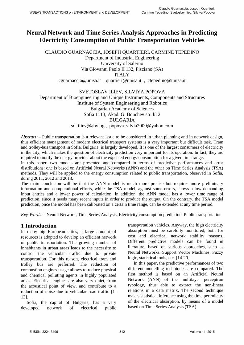
In Fig. 1 the multiple-correlation coefficients and

comparison between linear regression and ANN for

training, validation and testing are shown, while in

Fig. 2, the error histogram in the complete training

process is reported.



E-ISSN: 2224-3496 313 Volume 11, 2015

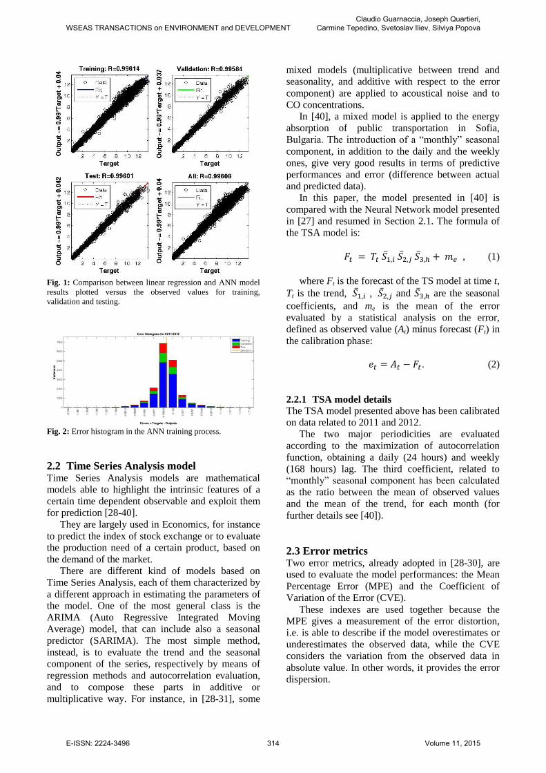
Fig. 1: Comparison between linear regression and ANN model

results plotted versus the observed values for training,

validation and testing.

Fig. 2: Error histogram in the ANN training process.

2.2 Time Series Analysis model Time Series Analysis models are mathematical

models able to highlight the intrinsic features of a

certain time dependent observable and exploit them

for prediction [28-40].

They are largely used in Economics, for instance

to predict the index of stock exchange or to evaluate

the production need of a certain product, based on

the demand of the market.

There are different kind of models based on

Time Series Analysis, each of them characterized by

a different approach in estimating the parameters of

the model. One of the most general class is the

ARIMA (Auto Regressive Integrated Moving

Average) model, that can include also a seasonal

predictor (SARIMA). The most simple method,

instead, is to evaluate the trend and the seasonal

component of the series, respectively by means of

regression methods and autocorrelation evaluation,

and to compose these parts in additive or

multiplicative way. For instance, in [28-31], some

mixed models (multiplicative between trend and

seasonality, and additive with respect to the error

component) are applied to acoustical noise and to

CO concentrations.

In [40], a mixed model is applied to the energy

absorption of public transportation in Sofia,

Bulgaria. The introduction of a “monthly” seasonal

component, in addition to the daily and the weekly

ones, give very good results in terms of predictive

performances and error (difference between actual

and predicted data).

In this paper, the model presented in [40] is

compared with the Neural Network model presented

in [27] and resumed in Section 2.1. The formula of

the TSA model is:

𝐹𝑡 = 𝑇𝑡 𝑆1̅,𝑖 𝑆2̅,𝑗 𝑆3̅,ℎ + 𝑚𝑒 , (1)

where Ft is the forecast of the TS model at time t,

Tt is the trend, 𝑆1̅,𝑖 , 𝑆2̅,𝑗 and 𝑆3̅,ℎ are the seasonal

coefficients, and me is the mean of the error

evaluated by a statistical analysis on the error,

defined as observed value (At) minus forecast (Ft) in

the calibration phase:

𝑒𝑡 = 𝐴𝑡 − 𝐹𝑡 . (2)

2.2.1 TSA model details

The TSA model presented above has been calibrated

on data related to 2011 and 2012.

The two major periodicities are evaluated

according to the maximization of autocorrelation

function, obtaining a daily (24 hours) and weekly

(168 hours) lag. The third coefficient, related to

“monthly” seasonal component has been calculated

as the ratio between the mean of observed values

and the mean of the trend, for each month (for

further details see [40]).

2.3 Error metrics Two error metrics, already adopted in [28-30], are

used to evaluate the model performances: the Mean

Percentage Error (MPE) and the Coefficient of

Variation of the Error (CVE).

These indexes are used together because the

MPE gives a measurement of the error distortion,

i.e. is able to describe if the model overestimates or

underestimates the observed data, while the CVE

considers the variation from the observed data in

absolute value. In other words, it provides the error

dispersion.



E-ISSN: 2224-3496 314 Volume 11, 2015

The two metrics are evaluated according to the

following formulas:

𝑀𝑃𝐸 =∑ (

𝐴𝑡−𝐹𝑡𝐴𝑡

)100𝑛𝑡=1

𝑛 (3)

and

𝐶𝑉𝐸 =√

∑ (𝑒𝑡)2𝑛𝑡=1

𝑛−1

�̅� , (4)

where At, Ft and et are the same as in formula (2), A̅

is the mean value of the actual data in the

considered time range, n is the number of data.

3 Comparison of the models Of course, since the models are deeply different, the

comparison must be carefully performed. In fact, it

is easy to foresee that the ANN model will be much

more efficient with respect to TSA. This is due to

the bigger number of parameters (day of the week

and of the month, hour, kilometers run, temperature,

etc.) and to the complexity of the ANN model, that

is designed to “learn” and “understand” the context

in which it is applied. On the contrary, the TSA

model has a very low number of inputs (only the

data in a certain past time range) and does not

consider many variables.

Thus, in the comparison, the authors will

underline that the choice of the proper predictive

model must be performed according to the needs of

the user: when a large accuracy is needed and there

are good computing platforms at disposal, the ANN

should be preferred, keeping in mind that, in order

to be used, it needs also information about

temperature, kilometers run, day of the week, etc..

On the contrary, if an average prediction is

satisfactory and the operator does not know all the

parameters needed for ANN model application, the

TSA model can give a good estimation, with low

mean error and standard deviation.

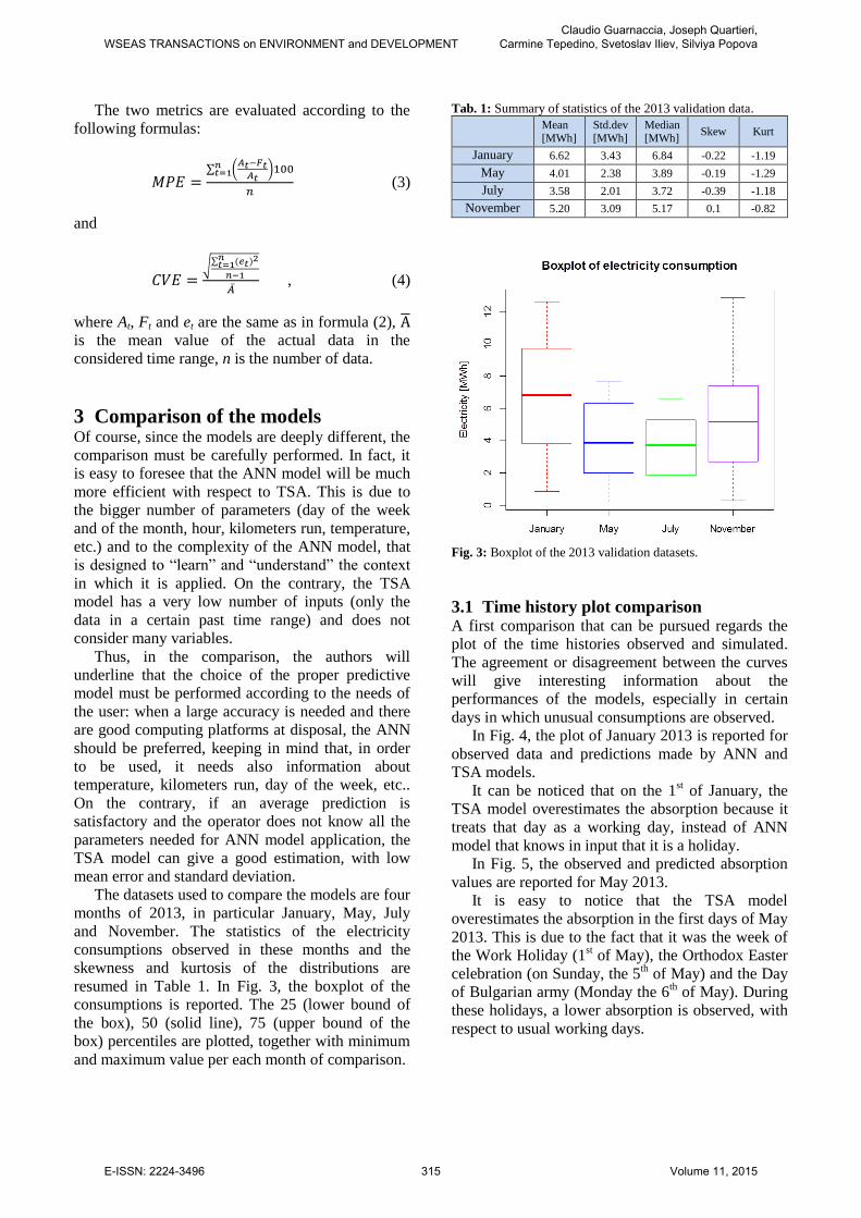
The datasets used to compare the models are four

months of 2013, in particular January, May, July

and November. The statistics of the electricity

consumptions observed in these months and the

skewness and kurtosis of the distributions are

resumed in Table 1. In Fig. 3, the boxplot of the

consumptions is reported. The 25 (lower bound of

the box), 50 (solid line), 75 (upper bound of the

box) percentiles are plotted, together with minimum

and maximum value per each month of comparison.

Tab. 1: Summary of statistics of the 2013 validation data.

Mean [MWh]

Std.dev [MWh]

Median [MWh]

Skew Kurt

January 6.62 3.43 6.84 -0.22 -1.19

May 4.01 2.38 3.89 -0.19 -1.29

July 3.58 2.01 3.72 -0.39 -1.18

November 5.20 3.09 5.17 0.1 -0.82

Fig. 3: Boxplot of the 2013 validation datasets.

3.1 Time history plot comparison A first comparison that can be pursued regards the

plot of the time histories observed and simulated.

The agreement or disagreement between the curves

will give interesting information about the

performances of the models, especially in certain

days in which unusual consumptions are observed.

In Fig. 4, the plot of January 2013 is reported for

observed data and predictions made by ANN and

TSA models.

It can be noticed that on the 1st of January, the

TSA model overestimates the absorption because it

treats that day as a working day, instead of ANN

model that knows in input that it is a holiday.

In Fig. 5, the observed and predicted absorption

values are reported for May 2013.

It is easy to notice that the TSA model

overestimates the absorption in the first days of May

2013. This is due to the fact that it was the week of

the Work Holiday (1st of May), the Orthodox Easter

celebration (on Sunday, the 5th of May) and the Day

of Bulgarian army (Monday the 6th of May). During

these holidays, a lower absorption is observed, with

respect to usual working days.



E-ISSN: 2224-3496 315 Volume 11, 2015

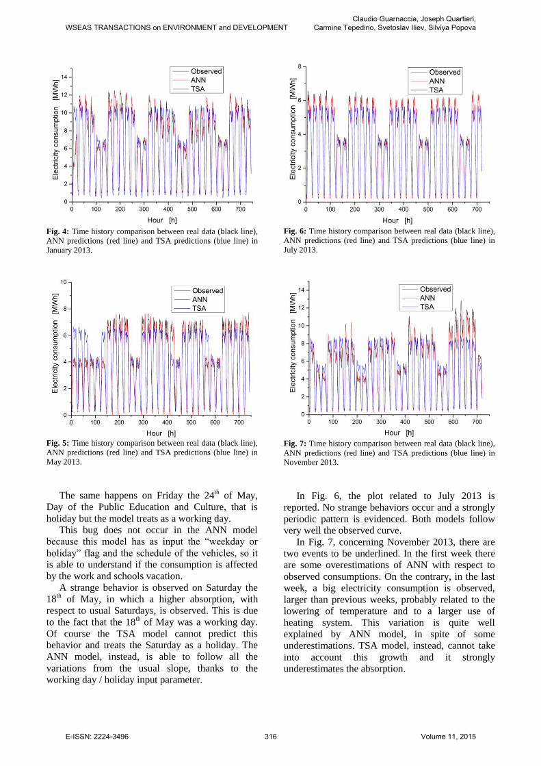
Fig. 4: Time history comparison between real data (black line),

ANN predictions (red line) and TSA predictions (blue line) in

January 2013.



May 2013.

The same happens on Friday the 24th of May,

Day of the Public Education and Culture, that is

holiday but the model treats as a working day.

This bug does not occur in the ANN model

because this model has as input the “weekday or

holiday” flag and the schedule of the vehicles, so it

is able to understand if the consumption is affected

by the work and schools vacation.

A strange behavior is observed on Saturday the

18th of May, in which a higher absorption, with

respect to usual Saturdays, is observed. This is due

to the fact that the 18th of May was a working day.

Of course the TSA model cannot predict this

behavior and treats the Saturday as a holiday. The

ANN model, instead, is able to follow all the

variations from the usual slope, thanks to the

working day / holiday input parameter.



July 2013.



November 2013.

In Fig. 6, the plot related to July 2013 is

reported. No strange behaviors occur and a strongly

periodic pattern is evidenced. Both models follow

very well the observed curve.

In Fig. 7, concerning November 2013, there are

two events to be underlined. In the first week there

are some overestimations of ANN with respect to

observed consumptions. On the contrary, in the last

week, a big electricity consumption is observed,

larger than previous weeks, probably related to the

lowering of temperature and to a larger use of

heating system. This variation is quite well

explained by ANN model, in spite of some

underestimations. TSA model, instead, cannot take

into account this growth and it strongly

underestimates the absorption.



E-ISSN: 2224-3496 316 Volume 11, 2015

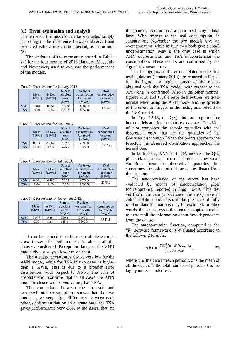
3.2 Error evaluation and analysis The error of the models can be evaluated simply

according to the difference between observed and

predicted values in each time period, as in formula

(2).

The statistics of the error are reported in Tables

2-5 for the four months of 2013 (January, May, July

and November) used to evaluate the performances

of the models.

Tab. 2: Error resume for January 2013.

Mean

[MWh]

St Dev

[MWh]

Sum of

absolute

error

[MWh]

Predicted

consumption

for month

[MWh]

Real

consumption

for month

[MWh]

ANN -0.076 0.361 204.81 4981.7 4924.7

TSA -0.04 1.16 607.96 4952.0

Tab. 3: Error resume for May 2013.

Mean

[MWh] St Dev [MWh]

Sum of

absolute error

[MWh]

Predicted

consumption for month

[MWh]

Real

consumption for month

[MWh]

ANN 0.017 0.3146 187.5 2969.6 2982.2

TSA -0.06 0.93 476.8 3027.9

Tab. 4: Error resume for July 2013.

Mean

[MWh]

St Dev

[MWh]

Sum of

absolute

error [MWh]

Predicted

consumption

for month [MWh]

Real

consumption

for month [MWh]

ANN 0.004 0.143 73.21 2572.9 2575.6

TSA 0.06 0.35 189.61 2533.5

Tab. 5: Error resume for November 2013.

Mean

[MWh]

St Dev

[MWh]

Sum of absolute

error

[MWh]

Predicted consumption

for month

[MWh]

Real consumption

for month

[MWh]

ANN -0.077 0.48 260.3 3803.1 3747.5

TSA -0.09 1.21 645.1 3809.2

It can be noticed that the mean of the error is

close to zero for both models, in almost all the

datasets considered. Except for January, the ANN

model gives always a lower mean error.

The standard deviation is always very low for the

ANN model, while for TSA in two cases is higher

than 1 MWh. This is due to a broader error

distribution, with respect to ANN. The sum of

absolute error confirms that in all cases the ANN

model is closer to observed values than TSA.

The comparison between the observed and

predicted total consumptions shows that the two

models have very slight differences between each

other, confirming that on an average base, the TSA

gives performances very close to the ANN, that, on

the contrary, is more precise on a local (single data)

base. With respect to the real consumption, in

January and November the two models give an

overestimation, while in July they both give a small

underestimation. May is the only case in which

ANN overestimates and TSA underestimates the

consumption. These results are confirmed by the

sign of the mean error.

The histograms of the errors related to the first

testing dataset (January 2013) are reported in Fig. 8.

In this figure, the higher spread of the results

obtained with the TSA model, with respect to the

ANN one, is confirmed. Also in the other months,

figures 9, 10 and 11, the error distributions are quite

normal when using the ANN model and the spreads

of the errors are bigger in the histograms related to

the TSA model.

In Figg. 12-15, the Q-Q plots are reported for

both models and for the four test datasets. This kind

of plot compares the sample quantiles with the

theoretical ones, that are the quantiles of the

Gaussian distribution. When the points approach the

bisector, the observed distribution approaches the

normal one.

In both cases, ANN and TSA models, the Q-Q

plots related to the error distributions show small

variations from the theoretical quantiles, but

sometimes the points of tails are quite distant from

the bisector.

The autocorrelation of the errors has been

evaluated by means of autocorrelation plots

(correlograms), reported in Figg. 16-19. This test

verifies if the data (in our case, the error) have an

autocorrelation and, if so, if the presence of fully

random data fluctuations may be excluded. In other

words, this test shows if the models adopted are able

to extract all the information about time dependence

from the dataset.

The autocorrelation function, computed in the

“R” software framework, is evaluated according to

the following formula:

r(k) = ∑ (xt−x̅)(xt+k−x̅)n−k

t=1

∑ (xt−nt=1 x̅)2 , (5)

where xt is the data in each period t, x̅ is the mean of

all the data, n is the total number of periods, k is the

lag hypothesis under test.



E-ISSN: 2224-3496 317 Volume 11, 2015

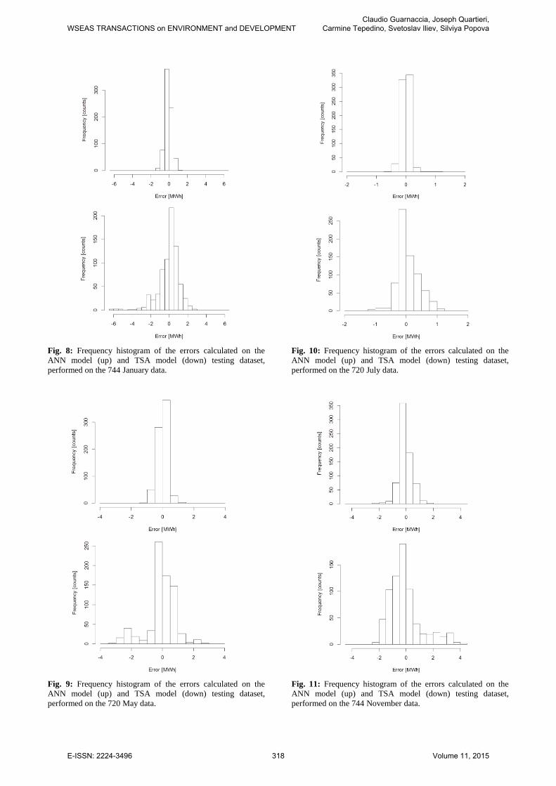
Fig. 8: Frequency histogram of the errors calculated on the

ANN model (up) and TSA model (down) testing dataset,

performed on the 744 January data.



performed on the 720 May data.



performed on the 720 July data.



performed on the 744 November data.



E-ISSN: 2224-3496 318 Volume 11, 2015

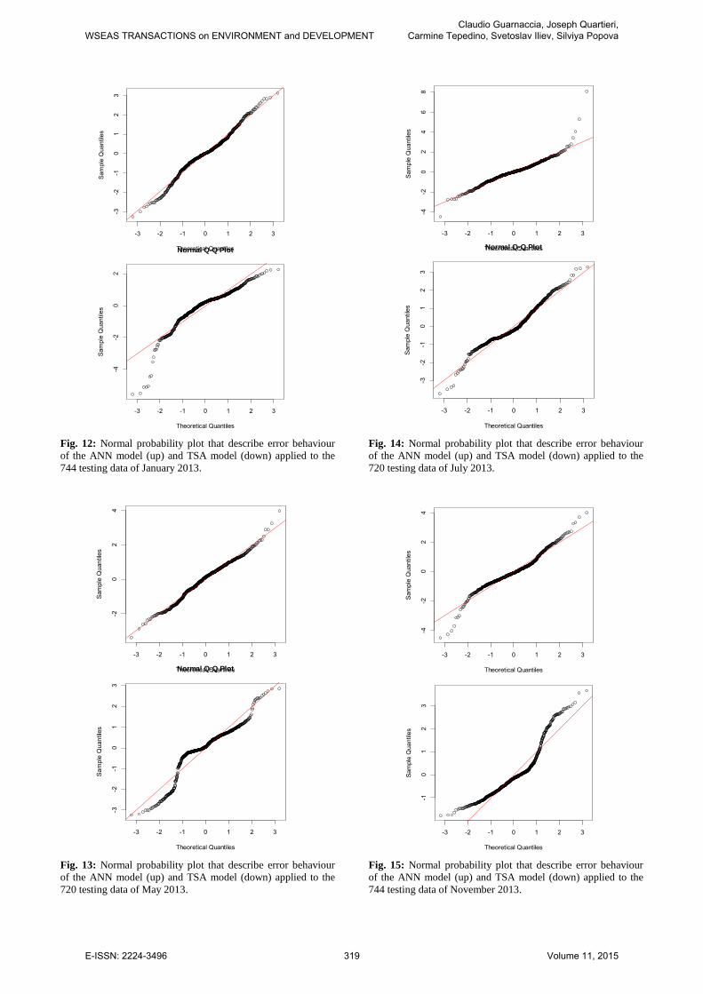
Fig. 12: Normal probability plot that describe error behaviour

of the ANN model (up) and TSA model (down) applied to the

744 testing data of January 2013.



720 testing data of May 2013.



720 testing data of July 2013.



744 testing data of November 2013.

-3 -2 -1 0 1 2 3

-3-2

-10

12

3

Normal Q-Q Plot

Theoretical Quantiles

Sam

ple

Qua

ntile

s

-3 -2 -1 0 1 2 3

-4-2

02

Normal Q-Q Plot


Sam

ple

Qua

ntile

s

-3 -2 -1 0 1 2 3

-20

24

Normal Q-Q Plot


Sam

ple

Qua

ntile

s

-3 -2 -1 0 1 2 3

-3-2

-10

12

3

Normal Q-Q Plot


Sam

ple

Qua

ntile

s

-3 -2 -1 0 1 2 3

-4-2

02

46

8

Normal Q-Q Plot


Sam

ple

Qua

ntile

s-3 -2 -1 0 1 2 3

-3-2

-10

12

3

Normal Q-Q Plot


Sam

ple

Qua

ntile

s

-3 -2 -1 0 1 2 3

-4-2

02

4

Normal Q-Q Plot


Sam

ple

Qua

ntile

s

-3 -2 -1 0 1 2 3

-10

12

3

Normal Q-Q Plot


Sam

ple

Qua

ntile

s



E-ISSN: 2224-3496 319 Volume 11, 2015

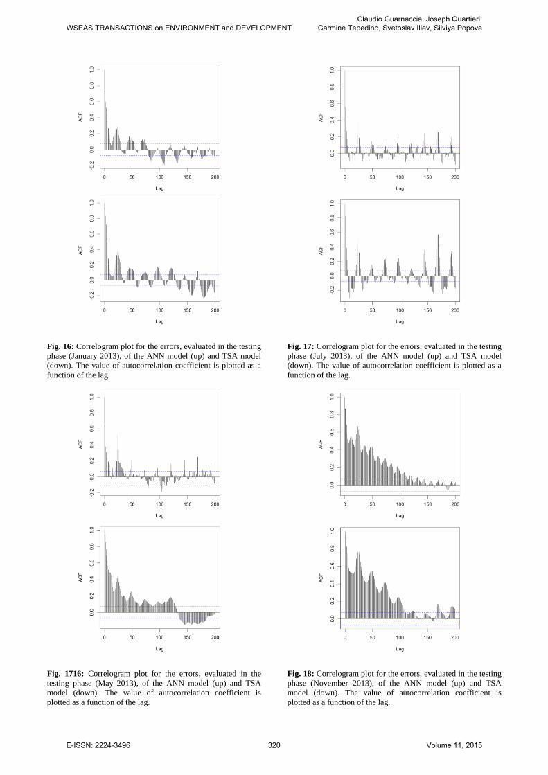
Fig. 16: Correlogram plot for the errors, evaluated in the testing

phase (January 2013), of the ANN model (up) and TSA model

(down). The value of autocorrelation coefficient is plotted as a

function of the lag.

Fig. 1716: Correlogram plot for the errors, evaluated in the

testing phase (May 2013), of the ANN model (up) and TSA

model (down). The value of autocorrelation coefficient is

plotted as a function of the lag.


phase (July 2013), of the ANN model (up) and TSA model

(down). The value of autocorrelation coefficient is plotted as a

function of the lag.


phase (November 2013), of the ANN model (up) and TSA

model (down). The value of autocorrelation coefficient is

plotted as a function of the lag.



E-ISSN: 2224-3496 320 Volume 11, 2015

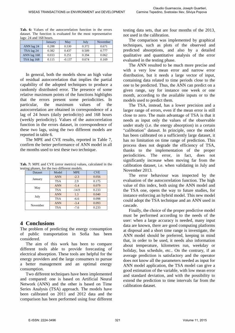
Tab. 6: Values of the autocorrelation function in the errors

dataset. The function is evaluated for the most representative

lags: 24 and 168 hours. January May July November

ANN lag 24 0.288 0.530 0.372 0.671

TSA lag 24 0.382 0.437 0.509 0.777

ANN lag 168 0.033 0.251 0.394 0.062

TSA lag 168 0.115 -0.137 0.674 0.169

In general, both the models show an high value

of residual autocorrelation that implies the partial

capability of the adopted techniques to produce a

randomly distributed error. The presence of some

relative maximum points of the functions highlights

that the errors present some periodicities. In

particular, the maximum values of the

autocorrelation are obtained in correspondence of a

lag of 24 hours (daily periodicity) and 168 hours

(weekly periodicity). Values of the autocorrelation

function in the errors dataset, in correspondence of

these two lags, using the two different models are

reported in table 6.

The MPE and CVE results, reported in Table 7,

confirm the better performance of ANN model in all

the months used to test these two technique.

Tab. 7: MPE and CVE (error metrics) values, calculated in the

testing phases, for the two different models. Dataset Model MPE CVE

January ANN -2.3 0.056

TSA 2.9 0.175

May ANN -5.4 0.079

TSA -14.9 0.233

July ANN 1.3 0.040

TSA -6.6 0.098

November ANN -3.4 0.093

TSA -7.6 0.233

4 Conclusions The problem of predicting the energy consumption

of public transportation in Sofia has been

considered.

The aim of this work has been to compare

different tools able to provide forecasting of

electrical absorption. These tools are helpful for the

energy providers and the large consumers to pursue

a better management and an optimal energy

consumption.

Two different techniques have been implemented

and compared: one is based on Artificial Neural

Network (ANN) and the other is based on Time

Series Analysis (TSA) approach. The models have

been calibrated on 2011 and 2012 data and the

comparison has been performed using four different

testing data sets, that are four months of the 2013,

not used in the calibration.

The comparison was implemented by graphical

techniques, such as plots of the observed and

predicted absorptions, and also by a detailed

qualitative and quantitative analysis of the error

evaluated in the testing phase.

The ANN resulted to be much more precise and

with a very low mean error and narrow error

distribution, but it needs a large vector of input,

containing data related to time periods close to the

one to be predicted. Thus, the ANN can predict on a

given range, say for instance one week or one

month, according to the available inputs or to the

models used to predict them.

The TSA, instead, has a lower precision and a

larger range of errors, even if the mean error is still

close to zero. The main advantage of TSA is that it

needs as input only the values of the observable

under study (i.e. the energy absorption) in a certain

“calibration” dataset. In principle, once the model

has been calibrated on a sufficiently large dataset, it

has no limitation on time range of prediction. This

process does not degrade the efficiency of TSA,

thanks to the implementation of the proper

periodicities. The error, in fact, does not

significantly increase when moving far from the

calibration dataset, i.e. when validating in July and

November 2013.

The error behaviour was inspected by the

evaluation of the autocorrelation function. The high

value of this index, both using the ANN model and

the TSA one, opens the way to future studies, for

instance enforcing an hybrid model. This new model

could adopt the TSA technique and an ANN used in

cascade.

Finally, the choice of the proper predictive model

must be performed according to the needs of the

user: when a large accuracy is needed, many input

data are known, there are good computing platforms

at disposal and a short time range is investigate, the

ANN model should be preferred, keeping in mind

that, in order to be used, it needs also information

about temperature, kilometres run, weekday or

holiday, bus schedule, etc.. On the contrary, if an

average prediction is satisfactory and the operator

does not know all the parameters needed as input for

ANN model application, the TSA model can give a

good estimation of the variable, with low mean error

and standard deviation, and with the possibility to

extend the prediction to time intervals far from the

calibration dataset.



E-ISSN: 2224-3496 321 Volume 11, 2015

References:

[1] Guarnaccia C., “Advanced Tools for Traffic

Noise Modelling and Prediction”, WSEAS

Transactions on Systems, Issue 2, Vol.12,

(2013) pp. 121-130.

[2] Quartieri J., Mastorakis N.E., Iannone G.,

Guarnaccia C., D’Ambrosio S., Troisi A.,

Lenza T.L.L., “A Review of Traffic Noise

Predictive Models”, Proc. of the 5th WSEAS

Int. Conf. on “Applied and Theoretical

Mechanics” (MECHANICS'09), Puerto de la

Cruz, Tenerife, Spain, December 14-16 2009,

pp. 72-80.

[3] Guarnaccia C., Lenza T.L.L., Mastorakis N.E.,

Quartieri J., “A Comparison between Traffic

Noise Experimental Data and Predictive

Models Results”, International Journal of

Mechanics, Issue 4, Vol. 5, (2011) pp. 379-386,

ISSN: 1998-4448.

[4] Guarnaccia C., “Analysis of Traffic Noise in a

Road Intersection Configuration”, WSEAS

Transactions on Systems, Issue 8, Volume 9,

(2010), pp.865-874, ISSN: 1109-2777.

[5] Iannone G., Guarnaccia C., Quartieri J., “Speed

Distribution Influence in Road Traffic Noise

Prediction”, Environmental Engineering And

Management Journal, Vol. 12, Issue 3, (2013)

pp. 493-501.

[6] Quartieri J., Iannone G., Guarnaccia C., “On

the Improvement of Statistical Traffic Noise

Prediction Tools”, Proc. of the 11th WSEAS

Int. Conf. on “Acoustics & Music: Theory &

Applications” (AMTA '10), Iasi, Romania, June

13-15 2010, pp. 201-207.

[7] Quartieri J., Mastorakis N.E., Guarnaccia C.,

Troisi A., D’Ambrosio S., Iannone G.,

“Traffic Noise Impact in Road Intersections”,

Int. Journal of Energy and Environment, Issue

1, Volume 4 (2010), pp. 1-8.

[8] Iannone G., Guarnaccia C., Quartieri J., “Noise

Fundamental Diagram deduced by Traffic

Dynamics”, in Recent Researches in

Geography, Geology, Energy, Environment and

Biomedicine, Proc. of the 4th WSEAS Int.

Conf. on Engineering Mechanics, Structures,

Engineering Geology (EMESEG ’11), Corfù

Island, Greece, July 14-16 2011, pp. 501-507.


Iannone G., “Cellular Automata Application to

Traffic Noise Control”, Proc. of the 12th Int.

Conf. on “Automatic Control, Modelling &

Simulation” (ACMOS '10), Catania (Italy),

May 29-31 2010, pp. 299-304.

[10] Guarnaccia C., “Acoustical Noise Analysis in

Road Intersections: a Case Study”, Proc. of the

11th WSEAS Int. Conf. on “Acoustics & Music:

Theory & Applications” (AMTA '10), Iasi,

Romania, June 13-15 2010, pp. 208-215.

[11] Guarnaccia C., “New Perspectives in Road

Traffic Noise Prediction”, in Latest advances in

Acoustics and Music, Proc. of the 13th Int.

Conf. on Acoustics & Music: Theory &

Applications (AMTA '12), Iasi, Romania, June

13-15 2012, pp. 255-260.


Troisi A., D’Ambrosio S., Iannone G., “Road

Intersections Noise Impact on Urban

Environment Quality”, Proc. of the 5th WSEAS

International Conference on “Applied and

Theoretical Mechanics” (MECHANICS '09),

Puerto de la Cruz, Tenerife, Spain, December

14-16 2009, pp. 162-171.

[13] Guarnaccia C., Quartieri J., Barrios J.M.,

Rodrigues E.R., “Modelling Environmental

Noise Exceedances Using non-Homogenous

Poisson Processes”, Journal of the Acoustical

Society of America, 136, (2014) pp. 1631-1639;

http://dx.doi.org/10.1121/1.4895662.

[14] Popova S., Iliev S., Trifonov M., Neural

Network Prediction of the Electricity

Consumption of Trolleybus and Tram

Transport in Sofia City, in Latest Trends in

Energy, Environment and Development, Proc.

of the Int. Conf. on Urban Planning and

Transportation (UPT’14), June 2014, Salerno

(Italy), pp. 116-120.

[15] Chen B.J., Chang M.W. and Lin C.J.. Load

Forecasting using Support Vector Machines: A

Study on EUNITE Competition 2001, Technical

report, Department of Computer Science and

Information Engineering, National Taiwan

University, 2002.

[16] Charytoniuk W., Chen M.S., and Van Olinda

P., Nonparametric Regression Based Short-

Term Load Forecasting, IEEE Transactions on

Power Systems, 13:725–730, 1998.

[17] Cho M.Y., Hwang J.C., and Chen C.S.,

Customer Short-Term Load Forecasting by

using ARIMA Transfer Function Model,

Proceedings of the International Conference on

Energy Management and Power Delivery,

1:317–322, 1995.

[18] Feinberg E.A., Hajagos J.T., and Genethliou

D., Statistical Load Modeling, Proc. of the 7th

IASTED International Multi-Conference:

Power and Energy Systems, 88–91, Palm

Springs, CA, 2003.

[19] Kiartzis S.J. and Bakirtzis A.G., A Fuzzy

Expert System for Peak Load Forecasting:

Application to the Greek Power System, Proc.



E-ISSN: 2224-3496 322 Volume 11, 2015

of the 10th Mediterranean Electrotechnical

Conference, 3:1097–1100, 2000.

[20] Calderaro V., Cogliano D., Galdi V., Graber

G., Piccolo A., An Algorithm to Optimize Speed

Profiles of the Metro Vehicles for Minimizing

Energy Consumption, in Power Electronics,

Electrical Drives, Automation and Motion

Ischia, Italy 18-20 June 2014 IEEE Pag.813-

819

[21] Thibault, J., Feedforward neural networks for

identification of dynamic processes, J. Chem.

Eng. Comm 105, 109-128, 1991.

[22] Thibault, J., Breusegem V.V. and Cheruy A.,

On line prediction of fermentation variables

using neural networks, J. Biotechnol. Bioeng.

36(12), 1041-1048, 1990.

[23] Thibault, J. and Cheruy A., A comparison of

GMDH and neural networks for modeling of a

bioprocess. In MIM-S2 Imacs Annals on

computing and applied mathematics

Proceedings, Sept., Brussels, 1990.

[24] Koprinkova P., Petrova M., Patarinska T.,

Bliznakova M., Neural Network Modelling of

Fermentation Processes. Specific Kinetic Rates

Models, Cybernetics and Systems: An

International Journal, vol. 29, N. 3, 1998,

pp.303-317.

[25] Petrova M., Koprinkova P., Patarinsaka T.,

Bliznakova M., Neural Network Modelling of

Fermentation Processes. Specific Growth Rate

Model, Bioprocess Engineering, vol.18, N. 4,

April 1998, pp.281-287.

[26] Petrova M., Koprinkova P., Patarinska T.,

Neural Network Model of Fermentation

Processes. Microorganisms Cultivation Model,

Bioprocess Engineering, vol.16, N. 3, Febr.

1997, pp.145-149.

[27] Iliev S., Popova S, Electricity Consumption

Prediction System for the Public

Transportation, WSEAS Transactions on

Systems, Vol.13, 2014, Art. #63, pp. 638-643.

[28] Guarnaccia C., Quartieri J., Mastorakis N.E.,

Tepedino C., Development and Application of

a Time Series Predictive Model to Acoustical

Noise Levels, WSEAS Transactions on

Systems, Vol. 13, (2014) pp. 745-756, ISSN /

E-ISSN: 1109-2777 / 2224-2678.

[29] Guarnaccia C., Quartieri J., Rodrigues E.R.,

Tepedino C., Acoustical Noise Analysis and

Prediction by means of Multiple Seasonality

Time Series Model, International Journal of

Mathematical Models and Methods in Applied

Sciences, Vol. 8, (2014) pp 384-393, ISSN:

1998-0140.

[30] Guarnaccia C., Cerón Bretón J.G., Quartieri J.,

Tepedino C., Cerón Bretón R.M., An

Application of Time Series Analysis for

Forecasting and Control of Carbon Monoxide

Concentrations, International Journal of

Mathematical Models and Methods in Applied

Sciences, Vol. 8, (2014) pp 505-515.

[31] Pope C.A., Dockery D.W., Spengler J.D., and

Raizenne M.E., Respiratory Health and

PM10 Pollution: A Daily Time Series Analysis,

American Review of Respiratory Disease,

Vol. 144, No. 3_pt_1, (1991) pp. 668-674.

[32] Dominici F., McDermott A., Zeger S.L., and

Samet J.M., On the Use of Generalized

Additive Models in Time-Series Studies of Air

Pollution and Health, American Journal of

Epidemiology, 156 (3), (2002) pp 193-203.

[33] Di Matteo T., Aste T., Dacorogna M.M.,

Scaling behaviors in differently developed

markets, Physica A: Statistical Mechanics and

its Applications, Vol. 324, Issues 1–2, (2003)

pp. 183-188.

[34] Milanato D., Demand Planning. Processi,

metodologie e modelli matematici per la

gestione della domanda commerciale, Springer,

Milano, 2008, in Italian.

[35] Chase R.B., Aquilano N.J., Operations

Management for Competitive Advantage, Irwin

Professional Pub, 10th edition, 2004.

[36] Guarnaccia C., Quartieri J., Mastorakis N. E.

and Tepedino C., Acoustic Noise Levels

Predictive Model Based on Time Series

Analysis, in “Latest Trends in Circuits,

Systems, Signal Processing and Automatic

Control”, Proc. of the 2nd

Int. Conf. on

Acoustics, Speech and Audio Processing

(ASAP'14), Salerno, Italy, June 3-5, 2014,

ISSN: 1790-5117, ISBN: 978-960-474-374-2,

pp. 140-147.

[37] Guarnaccia C., Quartieri J., Rodrigues E. R.

and Tepedino C., Time Series Model

Application to Multiple Seasonality Acoustical

Noise Levels Data Set, in “Latest Trends in

Circuits, Systems, Signal Processing and

Automatic Control”, Proc. of the 2nd

Int. Conf.

on Acoustics, Speech and Audio Processing

(ASAP'14), Salerno, Italy, June 3-5, 2014, pp.

171-180.

[38] Guarnaccia C., Quartieri J., Cerón Bretón J. G.,

Tepedino C., Cerón Bretón R. M., Time Series

Predictive Model Application to Air Pollution

Assessment, in “Latest Trends on Systems”,

Proc. of the 18th Int. Conf. on Circuits,

Systems, Communications and Computers



E-ISSN: 2224-3496 323 Volume 11, 2015

(CSCC'14), Santorini, Greece, 17-21 July 2014,

pp. 499-505.

[39] Tepedino C., Guarnaccia C., Iliev S., Popova

S., Quartieri J., Time Series Analysis and

Forecast of the Electricity Consumption of

Local Transportation, in “Recent Advances in

Energy, Environment and Financial Planning”,

Proc. of the 5th Int. Conf. on Development,

Energy, Environment, Economics (DEEE '14),

Firenze, Italy, 22-24 Nov 2014, pp. 13-22.

[40] Tepedino C., Guarnaccia C., Iliev S., Popova

S., Quartieri J., A Forecasting Model Based on

Time Series Analysis Applied to Electrical

Energy Consumption, accepted and in press,

International Journal of Mathematical Models

and Methods in Applied Sciences, 2015.

[41] Guarnaccia C., Quartieri J., Tepedino C.,

Rodrigues E. R., An analysis of airport noise

data using a non-homogeneous Poisson model

with a change-point, Applied Acoustics, Vol.

91, pp. 33-39, 2015.



E-ISSN: 2224-3496 324 Volume 11, 2015