


Languages
Pages
Legal

In the name of GodIn the name of God
Network Flows
7. Multicommodity Flows Problems
7.1 Introduction7.1 Introduction
Fall 2010Instructor: Dr. Masoud Yaghini
Introduction

Introduction
� In many application contexts, several physical
commodities, vehicles, or messages, each governed by
their own network flow constraints, share the same
network.
� If the commodities do not interact in any way, then to
solve problems with several commodities, we would solve problems with several commodities, we would
solve each single-commodity problem separately.
� In other situations, however, because the commodities
do share common facilities, the individual single
commodity problems are not independent, so to find
an optimal flow, we need to solve the problems in
concert with each other.
Introduction
� One such model, known as the multicommodity flow
problem, in which the individual commodities share
common arc capacities.
� That is, each arc has a capacity uij that restricts the
total flow of all commodities on that arc.
Introduction
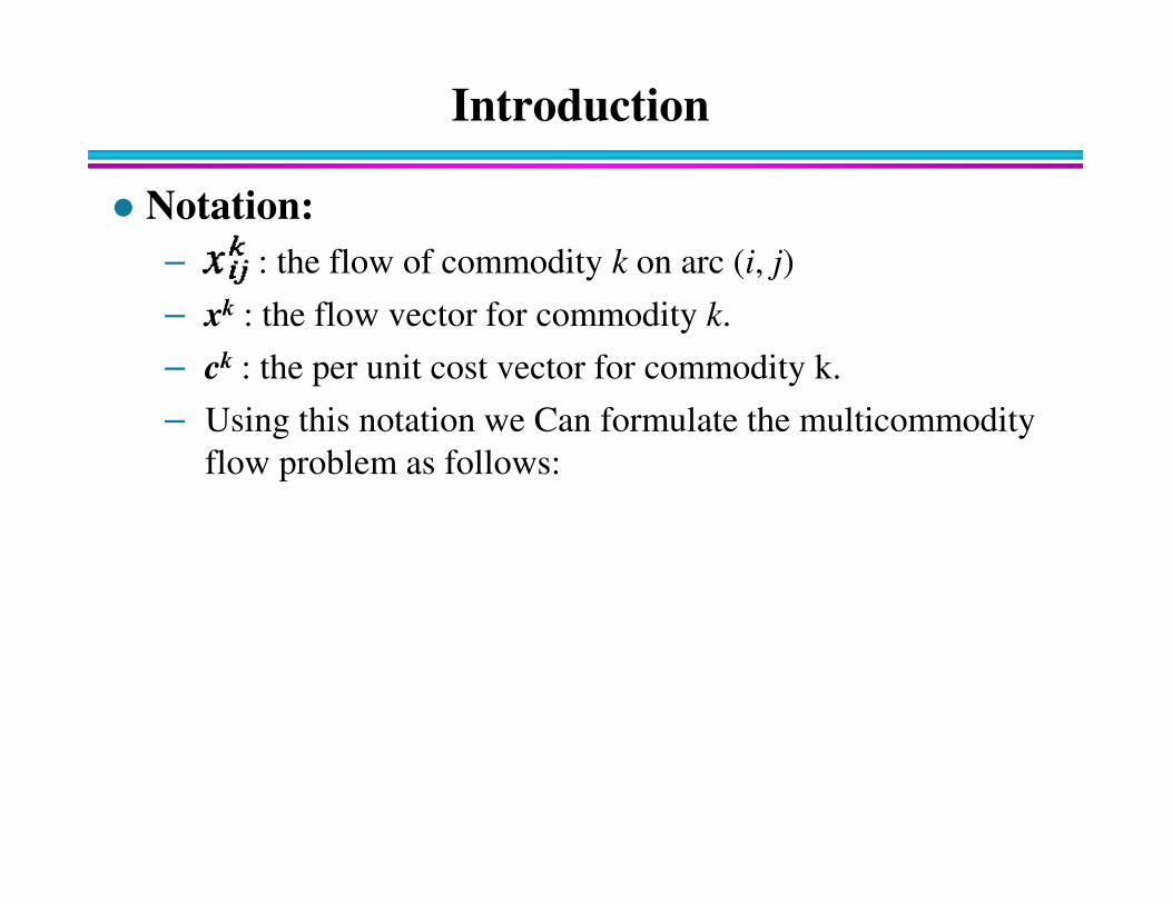
� Notation:
– : the flow of commodity k on arc (i, j)
– xk : the flow vector for commodity k.
– ck : the per unit cost vector for commodity k.
– Using this notation we Can formulate the multicommodity
flow problem as follows:flow problem as follows:
Introduction
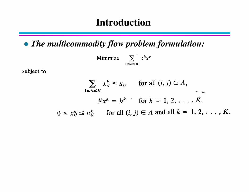
� The multicommodity flow problem formulation:

Introduction
� This formulation has a collection of K ordinary mass
balance constraints, modeling the flow of each
commodity k = 1, 2, . . . , K.
� The bundle constraints tie together the commodities
by restricting the total flow of all the commodities on
each arc (i, j) to at most uij.
Introduction
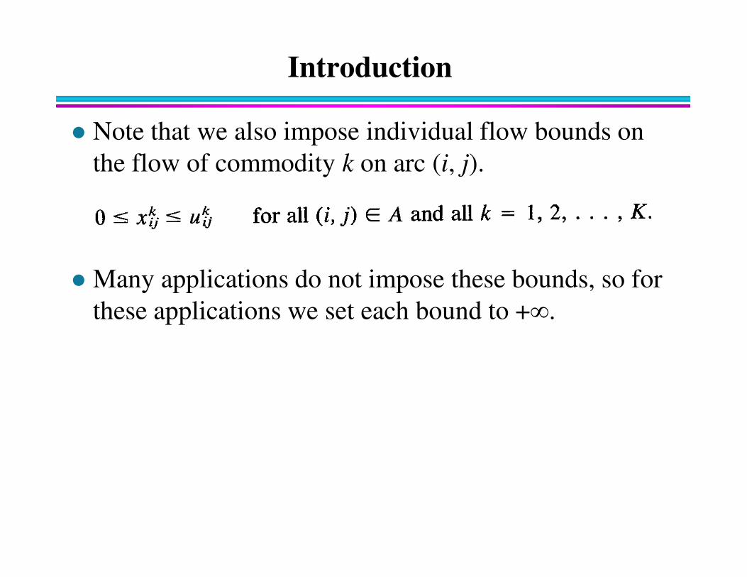
� Note that we also impose individual flow bounds on
the flow of commodity k on arc (i, j).
� Many applications do not impose these bounds, so for � Many applications do not impose these bounds, so for
these applications we set each bound to +∞.
Introduction
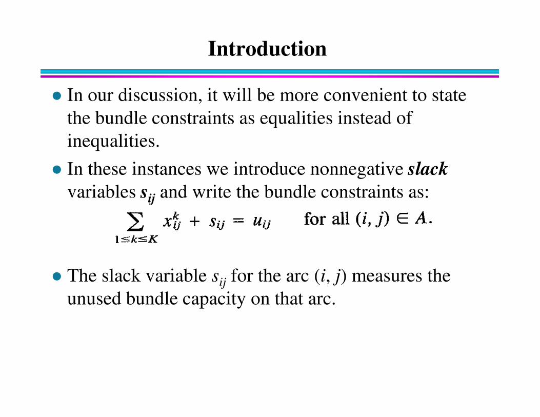
� In our discussion, it will be more convenient to state
the bundle constraints as equalities instead of
inequalities.
� In these instances we introduce nonnegative slack
variables sij and write the bundle constraints as:
� The slack variable sij for the arc (i, j) measures the
unused bundle capacity on that arc.

Assumptions
� The multicommodity flow model imposes capacities
on the arcs but not on the nodes.
� This modeling assumption imposes no loss of
generality, since by using the node splitting
techniques, we can use this formulation to model
situations with node capacities as well. situations with node capacities as well.
� Three assumptions are:
– Homogeneous goods assumption
– No congestion assumption
– Indivisible goods assumption

Assumptions
� Homogeneous goods assumption
– We are assuming that every unit flow of each commodity
uses 1 unit of capacity of each arc.
– A more general model would permit the unit flow of each
commodity k to consume a given amount of the capacity
associated with each arc (i, j), and replace the bundle associated with each arc (i, j), and replace the bundle
constraint with a more general resource availability
constraint:
Assumptions
� No congestion assumption
– We are assuming that we have a hard (i.e., fixed) capacity
on each arc and that the cost on each arc is linear in the
flow on that arc.
– In some applications as the flow of any commodity
increases on an arc, we incur an increasing and nonlinear increases on an arc, we incur an increasing and nonlinear
cost on that arc.
– For example, in traffic networks where the objective
function is to find the flow pattern of all the commodities
that minimizes overall system delay.
� In this setting, because of queuing effects, the greater the flow on
an arc, the greater is the queuing delay on that arc.
� This make the nonlinear multicommodity flow problems.

Assumptions
� Indivisible goods assumption
– The model assumes that the flow variables can be
fractional.
– In some applications the variables must be integer valued.
– In these instances the model that we are considering might
still prove to be useful, still prove to be useful,
� the linear programming model might either be a good
approximation of the integer programming model
� or we can use the linear programming model as a linear
programming relaxation of the integer program and embed it within
branch-and-bound approach.
Solution Approaches
� Researchers have developed several approaches for
solving the multicommodity flow problem, including:
– Price-directive decomposition methods
� Lagrangian Relaxation method
� Dantzig-Wolfe decomposition method
– Resource-directive decomposition methods – Resource-directive decomposition methods
– Partitioning methods

Solution Approaches
� Lagrangian Relaxation method
– bring bundle constraints into the objective function and
place Lagrangian multipliers or prices on them
– the resulting problem decomposes into a separate minimum
cost flow problem for each commodity k.
– These methods remove the capacity constraints and instead – These methods remove the capacity constraints and instead
charge each commodity for the use of the capacity of each
arc.
– These methods attempt to find appropriate prices so that
some optimal solution to the resulting pricing problem or
Lagrangian subproblem also solves the overall
multicommodity flow problem.
– Several methods are available for finding appropriate
prices.
Solution Approaches
� Dantzig-Wolfe decomposition method
– This is another approach for finding the correct prices;
– this method is a general-purpose approach for decomposing
problems that have a set of easy constraints and also a set
of hard constraints (that is, constraints that make the
problem much more difficult to solve). problem much more difficult to solve).
– For multicommodity flow problems, the network flow
constraints are the easy constraints and the bundle
constraints are the hard constraints.
– The approach begins by ignoring or imposing prices on the
bundle constraints and solving subproblems with only the
single-commodity network flow constraints.
Solution Approaches
� Dantzig-Wolfe decomposition method (cont.)
– The method uses linear programming to update the prices
so that the solutions generated from the subproblems satisfy
the bundle constraints.
– The method iteratively solves two different problems:
� A subproblem and � A subproblem and
� A price-setting linear program.

Solution Approaches
� Resource-directive decomposition methods
– These methods view the multicommodity flow problem as a
capacity allocation problem.
– All the commodities are competing for the fixed capacity uij
of every arc (i, j) of the network.
– Resource-directive methods begin by allocating the – Resource-directive methods begin by allocating the
capacities to the commodities, and
– Then use information collected from the solution to the
resulting single-commodity problems to reallocate the
capacities in a way that improves the overall system cost.
Solution Approaches
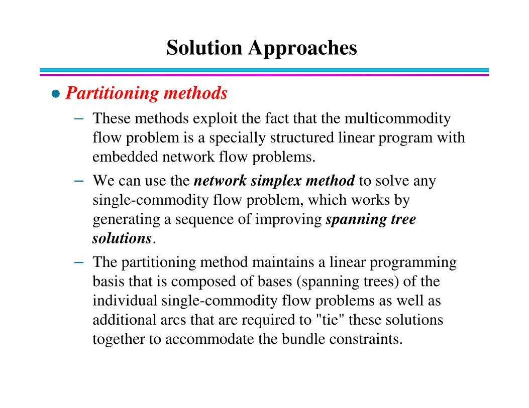
� Partitioning methods
– These methods exploit the fact that the multicommodity
flow problem is a specially structured linear program with
embedded network flow problems.
– We can use the network simplex method to solve any
single-commodity flow problem, which works by single-commodity flow problem, which works by
generating a sequence of improving spanning tree
solutions.
– The partitioning method maintains a linear programming
basis that is composed of bases (spanning trees) of the
individual single-commodity flow problems as well as
additional arcs that are required to "tie" these solutions
together to accommodate the bundle constraints.
Optimality Conditions
Optimality Conditions
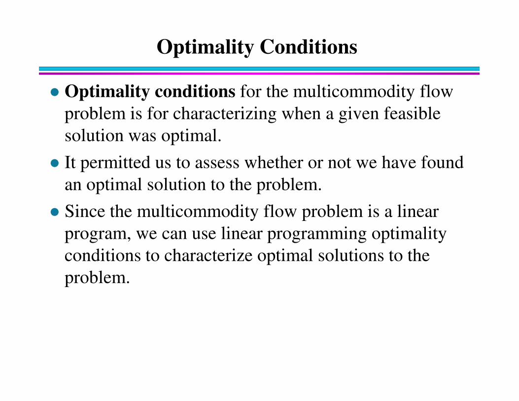
� Optimality conditions for the multicommodity flow
problem is for characterizing when a given feasible
solution was optimal.
� It permitted us to assess whether or not we have found
an optimal solution to the problem.
Since the multicommodity flow problem is a linear � Since the multicommodity flow problem is a linear
program, we can use linear programming optimality
conditions to characterize optimal solutions to the
problem.

Optimality Conditions
� The multicommodity flow problem formulation:

Optimality Conditions
� The multicommodity flow formulation has one bundle
constraint for every arc (i, j) of the network and one
mass balance constraint for each node-commodity
combination
� Types of dual variables of dual program :
– a price w on each arc (i, j)– a price wij on each arc (i, j)
– a node potential πk(i) for each combination of commodity
k and node i.

Optimality Conditions
� The dual of the multicommodity flow problem:
Optimality Conditions
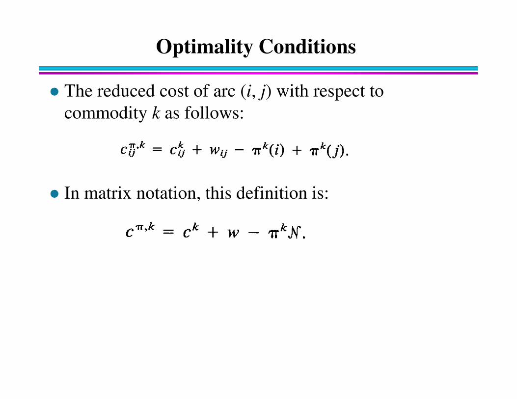
� The reduced cost of arc (i, j) with respect to
commodity k as follows:
� In matrix notation, this definition is:� In matrix notation, this definition is:
Optimality Conditions
� Complementary slackness (optimality) conditions
– The optimality conditions for a linear programming, called
the complementary slackness (optimality) conditions,
– It states that a primal feasible solution x and a dual feasible
solution (w, πk) are optimal to the respective problems if
and only if the product of each primal (dual) variable and and only if the product of each primal (dual) variable and
the slack in the corresponding dual (primal) constraint is
zero.
Optimality Conditions
� Multicommodity flow complementary slackness
conditions
– Let denote a specific value of the flow variable
– The commodity flows are optimal in the
multicommodity flow problem if and only if they are
feasible and for some choice of (nonnegative) arc prices wijfeasible and for some choice of (nonnegative) arc prices wij
and (unrestricted in sign) node potentials πk(i), the reduced
costs and arc flows satisfy the complementary slackness
conditions

Optimality Conditions
� Multicommodity flow complementary slackness
conditions

Optimality Conditions
� Condition (a)
– states that the price wij of arc (i, j) is zero if the optimal
solution does not use all of the capacity uij of the arc.
– That is, if the optimal solution does not fully use the
capacity of that arc, we could ignore the constraint (place
no price on it). no price on it).
� Optimal arc prices and optimal node potentials
– We refer to any set of arc prices and node potentials that
satisfy the complementary slackness conditions as optimal
arc prices and optimal node potentials.
Optimality Conditions
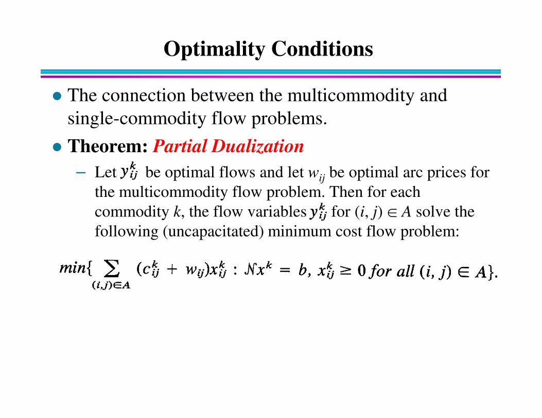
� The connection between the multicommodity and
single-commodity flow problems.
� Theorem: Partial Dualization
– Let be optimal flows and let wij be optimal arc prices for
the multicommodity flow problem. Then for each
commodity k, the flow variables for (i, j) œ A solve the commodity k, the flow variables for (i, j) œ A solve the
following (uncapacitated) minimum cost flow problem:

Optimality Conditions
� Proof.
– Since are optimal flows and wij are optimal arc prices for the
multicommodity flow problem, these variables together with
some set of node potentials πk(i) satisfy the complementary
slackness condition.
– The following conditions are the optimality conditions for the
uncapacitated minimum cost flow problem for commodity k with uncapacitated minimum cost flow problem for commodity k with
arc costs
– This observation implies that the flows solve the
corresponding minimum cost flow problems. .

The End
Top Related