


Languages
Pages
Legal


Natural language processing
(NLP)
From now on I will consider a language to be a set (finite or infinite) of sentences, each finite in
length and constructed out of a finite set of elements. All natural languages in their spoken
or written form are languages in this sense.
Noam Chomsky

Levels of processingSemantics
Focuses on the study of the meaning of words and the interactions between words to form larger units of meaning (such as sentences)
DiscourseBuilding on the semantic level, discourse analysis aims to determine the relationships between sentences
PragmaticsStudies how context, world knowledge, language conventions and other abstract properties contribute to the meaning of text 2

Evolution of translation
Word substituti
on
Linguistic analysis
Machine learning
3
NLP
Text is more difficult to process than numbersLanguage has many irregularitiesTypical speech and written text are not perfectDon’t expect perfection from text analysis
4

Sentiment analysis
A popular and simple method of measuring aggregate feelingGive a score of +1 to each “positive” word and -1 to each “negative” word Sum the total to get a sentiment score for the unit of analysis (e.g., tweet)
5
Shortcomings
IronyThe name of Britain’s biggest dog (until it died) was Tiny
SarcasmI started out with nothing and still have most of it left
Word analysis“Not happy” scores +1
6
Tokenization
Breaking a document into chunksTokensTypically wordsBreak at whitespace
Create a “bag of words”Many operations are at the word level
7
Terminology
NCorpus size Number of tokens
VVocabularyNumber of distinct tokens in the corpus
8

Count the number of words
library(stringr)# split a string into words into a list of wordsy <- str_split("The dead batteries were given out free of charge", " ")# report length of the vectorlength(y[[1]]) # double square bracket "[[]]" to reference a list member
9
R function for sentiment analysis
10
11
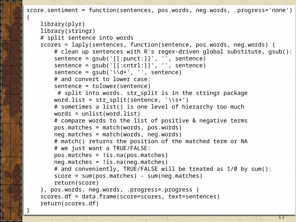
score.sentiment = function(sentences, pos.words, neg.words, .progress='none'){ library(plyr) library(stringr) # split sentence into words scores = laply(sentences, function(sentence, pos.words, neg.words) { # clean up sentences with R's regex-driven global substitute, gsub(): sentence = gsub('[[:punct:]]', '', sentence) sentence = gsub('[[:cntrl:]]', '', sentence) sentence = gsub('\\d+', '', sentence) # and convert to lower case: sentence = tolower(sentence) # split into words. str_split is in the stringr package word.list = str_split(sentence, '\\s+') # sometimes a list() is one level of hierarchy too much words = unlist(word.list) # compare words to the list of positive & negative terms pos.matches = match(words, pos.words) neg.matches = match(words, neg.words) # match() returns the position of the matched term or NA # we just want a TRUE/FALSE: pos.matches = !is.na(pos.matches) neg.matches = !is.na(neg.matches) # and conveniently, TRUE/FALSE will be treated as 1/0 by sum(): score = sum(pos.matches) - sum(neg.matches) return(score) }, pos.words, neg.words, .progress=.progress ) scores.df = data.frame(score=scores, text=sentences) return(scores.df)}
Sentiment analysis
Create an R script containing the score.sentiment functionSave the scriptRun the script
Compiles the function for use in other R scriptsLists under Functions in Environment
12

Sentiment analysis
13
# Sentiment examplesample = c("You're awesome and I love you", "I hate and hate and hate. So angry. Die!", "Impressed and amazed: you are peerless in your achievement of unparalleled mediocrity.")url <- "http://www.richardtwatson.com/dm6e/Reader/extras/positive-words.txt"hu.liu.pos <- scan(url,what='character', comment.char=';')url <- "http://www.richardtwatson.com/dm6e/Reader/extras/negative-words.txt"hu.liu.neg <- scan(url,what='character', comment.char=';')pos.words = c(hu.liu.pos)neg.words = c(hu.liu.neg)result = score.sentiment(sample, pos.words, neg.words)# reports score by sentence result$scoresum(result$score)mean(result$score)result$score

Text mining with tm
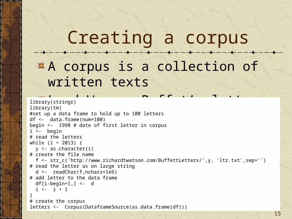
Creating a corpus
A corpus is a collection of written textsLoad Warren Buffet’s letters
15
library(stringr)library(tm)#set up a data frame to hold up to 100 lettersdf <- data.frame(num=100)begin <- 1998 # date of first letter in corpusi <- begin# read the letterswhile (i < 2013) { y <- as.character(i)# create the file name f <- str_c('http://www.richardtwatson.com/BuffettLetters/',y, 'ltr.txt',sep='')# read the letter as on large string d <- readChar(f,nchars=1e6)# add letter to the data frame df[i-begin+1,] <- d i <- i + 1}# create the corpusletters <- Corpus(DataframeSource(as.data.frame(df)))
Exercise
Create a corpus of Warren Buffet’s letters for 2008-2012
16
Readability
Flesch-KincaidAn estimate of the grade-level or years of education required of the reader• 13-16 Undergrad• 16-18 Masters• 19 - PhD
(11.8 * syllables_per_word) + (0.39 * words_per_sentence) - 15.59
17

koRpuslibrary(koRpus)#tokenize the first letter in the corpustagged.text <- tokenize(as.character(letters[[1]]), format="obj",lang="en")# scorereadability(tagged.text, "Flesch.Kincaid", hyphen=NULL,force.lang="en")
18

Exercise
What is the Flesch-Kincaid score for the 2010 letter?
19

Preprocessing
Case conversionTypically to all lower case
clean.letters <- tm_map(letters, content_transformer(tolower))
Punctuation removalRemove all punctuationclean.letters <- tm_map(clean.letters, content_transformer(removePunctuation))
Number filterRemove all numbersclean.letters <- tm_map(clean.letters, content_transformer(removeNumbers))
20

Preprocessing
Strip extra white spaceclean.letters <- tm_map(clean.letters, content_transformer(stripWhitespace))
Stop word filterclean.letters <- tm_map(clean.letters,removeWords,stopwords('SMART'))
Specific word removaldictionary <- c("berkshire","hathaway", "charlie", "million", "billion", "dollar")clean.letters <- tm_map(clean.letters,removeWords,dictionary)
21
Convert to lowercase before removing stop words
Preprocessing
Word filterRemove all words less than or greater than specified lengths
POS (parts of speech) filterRegex filterReplacer
Pattern replacer
22

Preprocessing
23
Sys.setenv(NOAWT = TRUE) # for Mac OS Xlibrary(tm)library(SnowballC)library(RWeka)library(rJava) library(RWekajars)# convert to lowerclean.letters <- tm_map(letters, content_transformer(tolower))# remove punctuationclean.letters <- tm_map(clean.letters,content_transformer(removePunctuation))# remove numbersclean.letters <- tm_map(clean.letters,content_transformer(removeNumbers))# remove stop words clean.letters <- tm_map(clean.letters,removeWords,stopwords('SMART'))# strip extra white spaceclean.letters <- tm_map(clean.letters,content_transformer(stripWhitespace))

Stemming
Reducing inflected (or sometimes derived) words to their stem, base, or root form
Banking to bankBanks to bank
24
stem.letters <- tm_map(clean.letters,stemDocument, language = "english")
Can take a while to
run

Frequency of words
A simple analysis is to count the number of termsExtract all the terms and place into a term-document matrix
One row for each term and one column for each document
25
tdm <- TermDocumentMatrix(stem.letters,control = list(minWordLength=3))dim(tdm)

Stem completionReturns stems to an original form to make text more readableUses original document as the dictionarySeveral options for selecting the matching word
prevalent, first, longest, shortestTime consuming so don't apply to the corpus but the term-document matrix
26
tdm.stem <- stemCompletion(rownames(tdm), dictionary=clean.letters, type=c("prevalent"))# change to stem completed row namesrownames(tdm) <- as.vector(tdm.stem)
Will take minutes to run
Frequency of words
Report the frequencyfindFreqTerms(tdm, lowfreq = 100, highfreq = Inf)
27

Frequency of words (alternative)
Extract all the terms and place into a document-term matrix
One row for each document and one column for each term
dtm <- DocumentTermMatrix(stem.letters,control = list(minWordLength=3))dtm.stem <- stemCompletion(rownames(dtm), dictionary=clean.letters, type=c("prevalent"))rownames(dtm) <- as.vector(dtm.stem)
Report the frequencyfindFreqTerms(dtm, lowfreq = 100, highfreq = Inf)
28

Exercise
Create a term-document matrix and find the words occurring more than 100 times in the letters for 2008-2102
Do appropriate preprocessing
29
Frequency
Term frequency (tf)Words that occur frequently in a document represent its meaning well
Inverse document frequency (idf)Words that occur frequently in many documents aren’t good at discriminating among documents
30
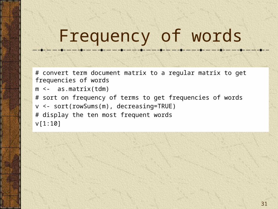
Frequency of words
# convert term document matrix to a regular matrix to get frequencies of wordsm <- as.matrix(tdm)# sort on frequency of terms to get frequencies of wordsv <- sort(rowSums(m), decreasing=TRUE)# display the ten most frequent wordsv[1:10]
31

Exercise
Report the frequency of the 20 most frequent words
Do several runs to identify words that should be removed from the top 20 and remove them
32

Probability densitylibrary(ggplot2)# get the names corresponding to the wordsnames <- names(v)# create a data frame for plottingd <- data.frame(word=names, freq=v)ggplot(d,aes(freq)) + geom_density(fill="salmon") + xlab("Frequency")
33

Word cloud
34
library(wordcloud)# select the color palettepal = brewer.pal(5,"Accent")# generate the cloud based on the 30 most frequent wordswordcloud(d$word, d$freq, min.freq=d$freq[30],colors=pal)

Exercise
Produce a word cloud for the words identified in the prior exercise
35
Co-occurrence
Co-occurrence measures the frequency with which two words appear togetherIf two words both appear or neither appears in same document
Correlation = 1
If two words never appear together in the same document
Correlation = -136
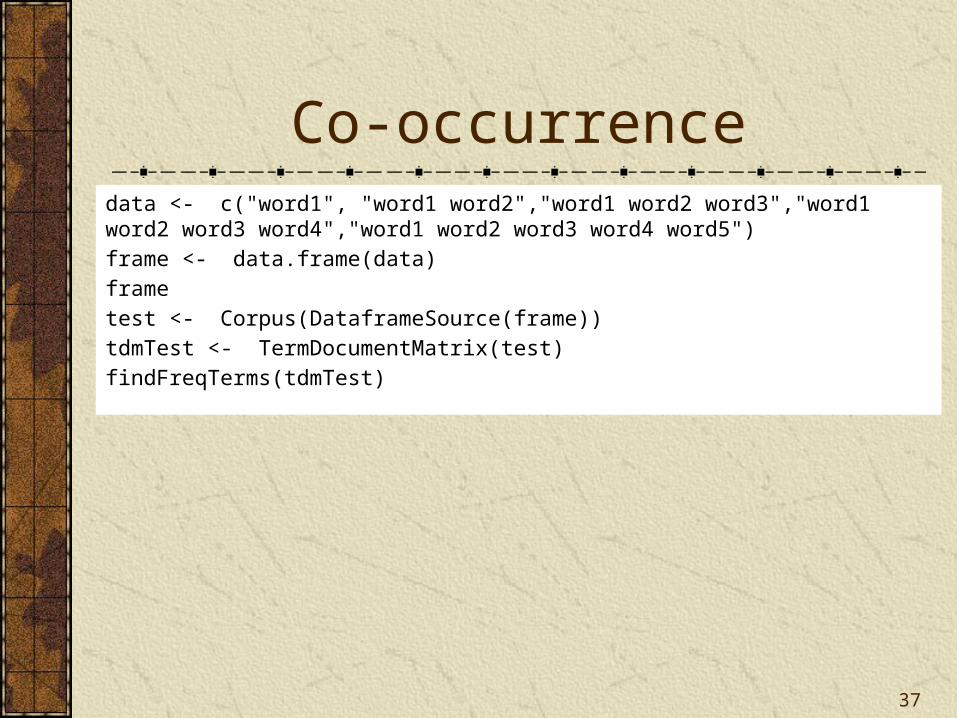
Co-occurrencedata <- c("word1", "word1 word2","word1 word2 word3","word1 word2 word3 word4","word1 word2 word3 word4 word5")frame <- data.frame(data)frametest <- Corpus(DataframeSource(frame))tdmTest <- TermDocumentMatrix(test)findFreqTerms(tdmTest)
37

Co-occurrence matrix
1 2 3 4 5
word1 1 1 1 1 1
word2 0 1 1 1 1
word3 0 0 1 1 1
word4 0 0 0 1 1
word5 0 0 0 0 1
38
Document
Note that co-occurrence is at the document level
> # Correlation between word2 and word3, word4, and word5> cor(c(0,1,1,1,1),c(0,0,1,1,1))[1] 0.6123724> cor(c(0,1,1,1,1),c(0,0,0,1,1))[1] 0.4082483> cor(c(0,1,1,1,1),c(0,0,0,0,1))[1] 0.25

Association
Measuring the association between a corpus and a given termCompute all correlations between the given term and all terms in the term-document matrix and report those higher than the correlation threshold
39

Find Association
Computes correlation of columns to get association
# find associations greater than 0.1findAssocs(tdmTest,"word2",0.1)
40

Find Association
# compute the associationsfindAssocs(tdm, "investment",0.90)
41
shooting cigarettes eyesight feed moneymarket pinpoint 0.83 0.82 0.82 0.82 0.82 0.82 ringmaster suffice tunnels unnoted 0.82 0.82 0.82 0.82

Exercise
Select a word and compute its association with other words in the Buffett letters corpus
Adjust the correlation coefficient to get about 10 words
42

Cluster analysis
Assigning documents to groups based on their similarity
Google uses clustering for its news site
Map frequent words into a multi-dimensional spaceMultiple methods of clusteringHow many clusters?
43

Clustering
The terms in a document are mapped into n-dimensional space
Frequency is used as a weight
Similar documents are close together
Several methods of measuring distance
44

Cluster analysis
45
library(ggplot2)library(ggdendro)# name the columns for the letter's yearcolnames(tdm) <- 1998:2012# Remove sparse termstdm1 <- removeSparseTerms(tdm, 0.5) # transpose the matrixtdmtranspose <- t(tdm1) cluster = hclust(dist(tdmtranspose),method='centroid')# get the clustering datadend <- as.dendrogram(cluster) # plot the treeggdendrogram(dend,rotate=T)

Cluster analysis
46
Exercise
Review the documentation of the hclust function in the stats package and try one or two other clustering techniques
47

Topic modeling
Goes beyond the independent bag-of-words approach to consider the order of wordsTopics are latent (hidden)The number of topics is fixed in advanceInput is a document term matrix
48
Topic modeling
Some methodsLatent Dirichlet allocation (LDA)Correlated topics model (CTM)
49
Identifying topics
Words that occur frequently in many documents are not good differentiatorsThe weighted term frequency inverse document frequency (tf-idf) determines discriminators Based on term frequency (tf) inverse document frequency (idf) 50

Inverse document frequency (idf)
idf measures the frequency of a term across documents
If a term occurs in every document
idf = 0
If a term occurs in only one document out of 15
idf = 3.91 51
m = number of documentsdft = number of documents with term t

Inverse document frequency (idf)
52
More than 5,000 terms in only in one document
Less than 500 terms in all documents

Term frequency inverse document frequency (tf-
idf)
Multiply a term’s frequency (tf) by its inverse document frequency (idf)
53
tftd = frequency of term t in document d
Topic modeling
Pre-process in the usual fashion to create a document-term matrixReduce the document-term matrix to include terms occurring in a minimum number of documents
54
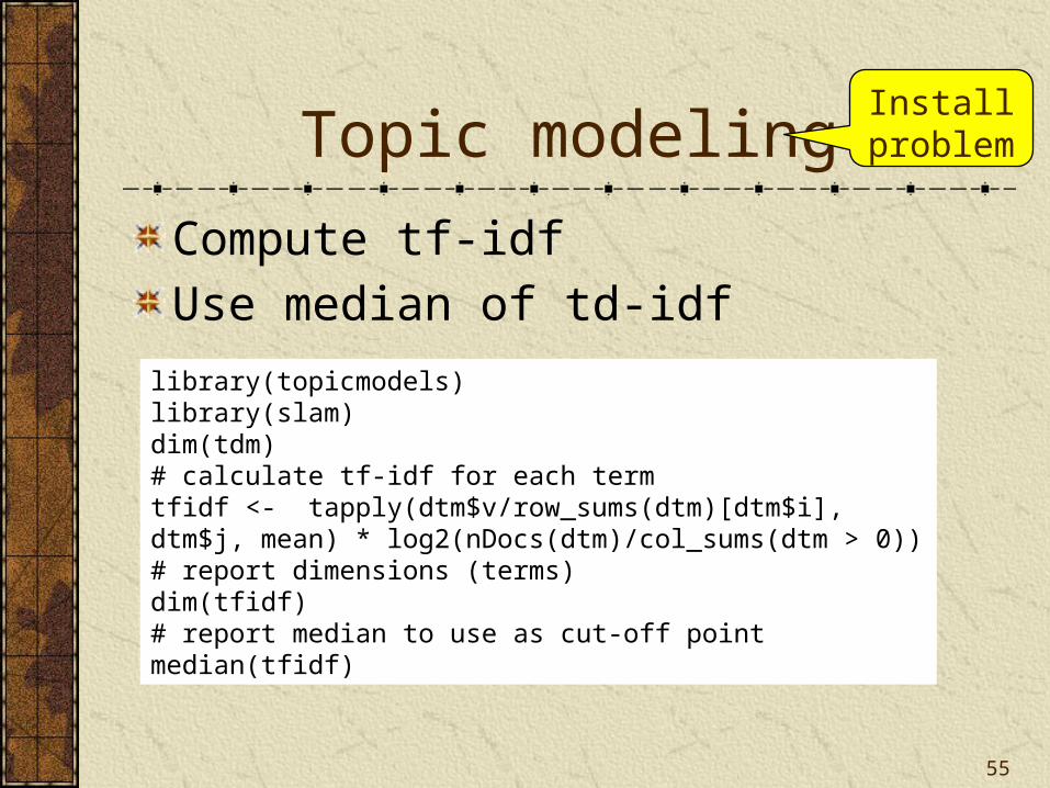
Topic modeling
Compute tf-idfUse median of td-idf
55
library(topicmodels)library(slam)dim(tdm)# calculate tf-idf for each termtfidf <- tapply(dtm$v/row_sums(dtm)[dtm$i], dtm$j, mean) * log2(nDocs(dtm)/col_sums(dtm > 0))# report dimensions (terms)dim(tfidf)# report median to use as cut-off pointmedian(tfidf)
Install problem

Topic modeling
Omit terms with a low frequency and those occurring in many documents
56
# select columns with tfidf > mediandtm <- dtm[, tfidf >= median(tfidf)]#select rows with rowsum > 0dtm <- dtm[row_sums(dtm) > 0,]# report reduced dimensiondim(dtm)
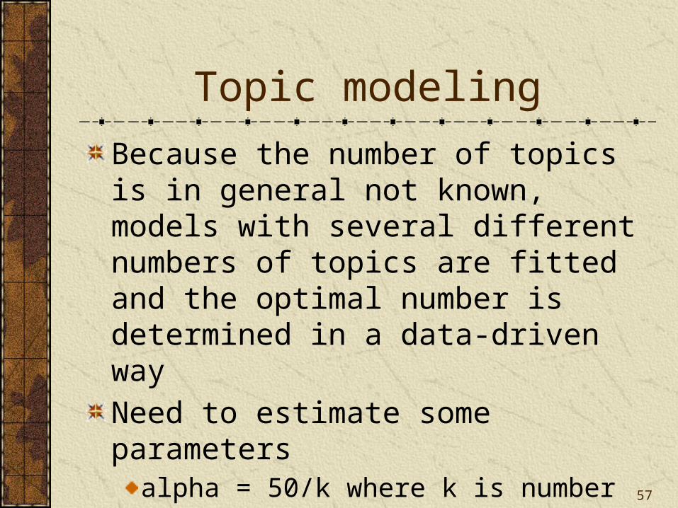
Topic modeling
Because the number of topics is in general not known, models with several different numbers of topics are fitted and the optimal number is determined in a data-driven wayNeed to estimate some parameters
alpha = 50/k where k is number of topicsdelta = 0.1
57

Topic modeling# set number of topics to extractk <- 5SEED <- 2010# try multiple methods – takes a while for a big corpusTM <- list(VEM = LDA(dtm, k = k, control = list(seed = SEED)), VEM_fixed = LDA(dtm, k = k, control = list(estimate.alpha = FALSE, seed = SEED)), Gibbs = LDA(dtm, k = k, method = "Gibbs", control = list(seed = SEED, burnin = 1000, thin = 100, iter = 1000)), CTM = CTM(dtm, k = k,control = list(seed = SEED, var = list(tol = 10^-3), em = list(tol = 10^-3))))
58

Examine results for meaningfulness
59
> topics(TM[["VEM"]], 1) 1 2 3 4 5 6 7 8 9 10 11 12 13 14 15 4 4 4 2 2 5 4 4 4 3 3 5 1 5 5 > terms(TM[["VEM"]], 5) Topic 1 Topic 2 Topic 3 Topic 4 Topic 5 [1,] "thats" "independent" "borrowers" "clayton" "clayton"[2,] "bnsf" "audit" "clayton" "eja" "bnsf" [3,] "cant" "contributions" "housing" "contributions" "housing"[4,] "blackscholes" "reserves" "bhac" "merger" "papers" [5,] "railroad" "committee" "derivative" "reserves" "marmon"

Named Entity Recognition (NER)
Identifying some or all mentions of people, places, organizations, time and numbers
60
The Olympics were in London in 2012.
Organization
Place
Date
The <organization>Olympics</organization> were in <place>London</place> in <date>2012</date>.
Rules-based approach
Appropriate for well-understood domainsRequires maintenanceLanguage dependent
61
Statistical classifiers
Look at each word in a sentence and decide
Start of a named-entityContinuation of an already identified named-entityNot part of a named-entity
Identify type of named-entityNeed to train on a collection of human-annotated text
62
Machine learning
Annotation is time-consuming but does not require a high-level of skillThe classifier needs to be trained on approximately 30,000 wordsA well-trained system is usually capable of correctly recognizing entities with 90% accuracy
63
OpenNLP
Comes with an NER toolRecognizes
PeopleLocationsOrganizationsDatesTimesPercentagesMoney
64

OpenNLP
The quality of an NER system is dependent on the corpus used for trainingFor some domains, you might need to train a modelOpenNLP useshttp://www-nlpir.nist.gov/related_projects/muc/proceedings/muc_7_toc.html
65
NER
Mostly implemented with Java codeR implementation is not cross platformKNIME offers a GUI “Lego” kit
Output is limitedDocumentation is limited
66
KNIME
KNIME (Konstanz Information Miner)General purpose data management and analysis package
67
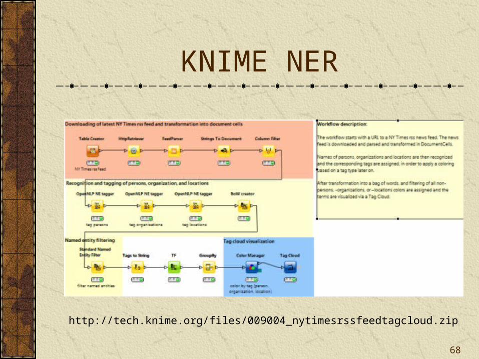
KNIME NER
68
http://tech.knime.org/files/009004_nytimesrssfeedtagcloud.zip
Further developments
Document summarizationRelationship extraction
Linkage to other documents
Sentiment analysisBeyond the naïve
Cross-language information retrieval
Chinese speaker querying English documents and getting a translation of the search and selected documents 69

Conclusion
Text mining is a mix of science and art because natural text is often imprecise and ambiguousManage your clients’ expectationsText mining is a work in progress so continually scan for new developments
70
Top Related