


Languages
Pages
Legal


NBER WORKING PAPER SERIES
PASS-THROUGH OF OIL PRICES TO JAPANESE DOMESTIC PRICES
Etsuro ShiojiTaisuke Uchino
Working Paper 15888http://www.nber.org/papers/w15888
NATIONAL BUREAU OF ECONOMIC RESEARCH1050 Massachusetts Avenue
Cambridge, MA 02138April 2010
A part of this paper is based on research we have conducted at the Research and Statistics Departmentof the Bank of Japan. We would like to thank members of the Department, especially Kazuo Monma,Munehisa Kasuya and Masahiro Higo for helpful comments and discussions on our research. We alsothank Takatoshi Ito for insightful suggestions at an early stage of this research. We are grateful toparticipants of the 20th East Asian Economic Seminar (Hong Kong, June 26-27, 2009), especiallythe discussants Donghyun Park and Yuko Hashimoto, as well as the organizers (Andrew Rose andTakatoshi Ito) for many invaluable comments that have led to substantial improvement of the paper.We also would like to thank two anonymous referees for their insightful comments. Shioji thanks financialassistance from the “Understanding Inflation Dynamics of the Japanese Economy” project of HitotsubashiUniversity, and Uchino thanks the Global COE Grant “Research unit for statistical and empirical analysisin social sciences” of Hitotsubashi University. The views expressed herein are those of the authorsand do not necessarily reflect the views of the National Bureau of Economic Research.
NBER working papers are circulated for discussion and comment purposes. They have not been peer-reviewed or been subject to the review by the NBER Board of Directors that accompanies officialNBER publications.
© 2010 by Etsuro Shioji and Taisuke Uchino. All rights reserved. Short sections of text, not to exceedtwo paragraphs, may be quoted without explicit permission provided that full credit, including © notice,is given to the source.

Pass-Through of Oil Prices to Japanese Domestic PricesEtsuro Shioji and Taisuke UchinoNBER Working Paper No. 15888April 2010JEL No. E31,F41,O53,Q43
ABSTRACT
In this paper, we investigate changes in the impacts of world crude oil prices on domestic prices inJapan. First, we employ a time-varying parameter VAR (TVP-VAR) approach to confirm that therate of pass-through of oil prices declined, both at the aggregate and sectoral levels, for the period1980-2000. Second, by utilizing Input-Output Tables, we find that changing cost structure of Japanesefirms goes a long way toward explaining this decline. That is, by the year 2000, oil had become a muchsmaller component of the Japanese production cost structure. We further find that much of this is attributableto changes in relative prices: as oil became cheaper, it became less important in the overall cost structure,and thus pricing behaviors of firms became less responsive to its prices. Substitution effects, namelyfirms’ shifts toward less oil intensive production, on the other hand, appear to be less important. Wealso study the period 2000-2007. We find that, although pass-through rates of oil prices increase inmany instances, those increases are small in comparison to the drastic resurgence of oil in the coststructure of firms. We present some possible explanations for this finding.
Etsuro ShiojiDepartment of EconomicsHitotsubashi University2-1 Naka, KunitachiTokyo [email protected]
Taisuke UchinoGCOE FellowGraduate School of EconomicsHitotsubashi [email protected]

3
1 Introduction
This paper studies the effects of oil prices on domestic prices using the Japanese data. Recent
dramatic surge and fall of crude oil prices have renewed interest in their effects on domestic
economies. In the literature, many authors have documented (in many cases using the US data)
weakening impacts of oil prices on the domestic economy. For example, Hooker (1996) finds
that impacts of oil prices on US GDP and US unemployment have diminished since the mid
1970s. Hooker (2002), which is more relevant for the current analysis, finds that the impact of oil
prices on US domestic inflation has been weakened significantly since around 1980. De
Gregorio, Landerretche, and Neilson (2007) apply a Hooker-type approach to a number of
industrialized as well as developing countries and confirm his findings. They also estimate
rolling VARs for those countries and again confirm declines in oil price pass-through. Blanchard
and Gali (2007) also estimate rolling VARs for the US. They also estimate regular VARs for the
US and other industrialized countries, splitting the sample at 1984. They arrive at similar
conclusions as the previous authors2. Causes behind these changes have also attracted attention
of macroeconomists. As Blinder and Rudd (2009) summarize succinctly, three possible
candidates have been widely considered. First is increased credibility of monetary policy. Second
is greater wage flexibility. Third is changing industrial structure after the two oil crises, i.e., the
substitution effects: firms have shifted away from energy using technology to energy saving
technology3,4. 2 However, they find inexplicable impulse response results for Japan. 3 Blanchard and Gali (2007) construct a New Keynesian DSGE model that incorporates all three elements. Their simulations show that all three have contributed to declining pass-through of oil prices. Kilian (2008) mentions two other candidates: one is a US specific reason (structure of the automobile industry) which is less relevant here. The other is a difference in the fundamental causes behind different episodes of oil price surges: it is hypothesized that the oil price increase in the 2000s was a consequence of a world wide demand increase rather than a supply shock. For inflation, however, it is not clear if demand-driven oil price increase should have either stronger or weaker effects on domestic prices. De Gregorio et. al. (2007) argue that a positive demand shock would tend to appreciate currencies of commodity importing countries, thus mitigating the effects of higher oil prices. De Gregorio et. al. (2007) also offer an additional candidate for the cause of the pass-through decline: under a low inflation environment, firms change prices less frequently, and, as a consequence, oil price increases are not easily passed through to domestic prices. 4 Another important hypothesis is that oil prices were not so influential to begin with: it was another shock that occurred around the same time period that had much impact on the economy (the most notable candidate is an excessively tight monetary policy). Refer to, for example, Bernanke, Gertler and Watson (1997). Blinder and Rudd (2008), on the other hand, support the supply-shock view of the “Great Inflation” of the 1970s and the 1980s.

4
In this paper, we study the Japanese data using time series analysis technique and confirm the
tendency of declining pass-through of oil prices to domestic prices, for the period 1980-2000.
We find that the main driving force behind this was different from any of the above three.
Investigation of the Japanese Input-Output tables reveals that changes in the cost structure alone
go a long way toward explaining the declining pass-through. In that sense, at a first glance, our
results might seem consistent with the third hypothesis mentioned above. But a further analysis
indicates that the main reason behind the changing cost structure was not the substitution effects
or changes in relative quantities: it was rather changes in the relative prices that played a more
important role. Put simply, as oil became cheaper, it became less and less important in the overall
cost structure (due partially to a relatively low degree of substitution between oil and non-oil
inputs), and thus the pricing behaviors of the firms became less responsive to its prices. The real
factor or the substitution effect did play some role, mainly in the short run, but its role in the long
term decline in the pass-through rate was relatively minor (with some exceptions, such as the
electricity sector)5. We also document the importance of taking into account features of the
Japanese oil-related taxation system.
This paper is a sequel to Shioji and Uchino (2009). In that paper, we estimate a series of VARs
with oil prices, the exchange rate, and various indicators of domestic prices, splitting the entire
sample period into two sub-periods: the first is the period February 1976 to December 1989, and
the second is from January 1990 to January 2009. It is reported that, as a general tendency,
pass-through of both oil prices and the exchange rate tend to decline between the two periods.
Then, those results are compared to the results of our study on the Japanese input-output table,
though we use only information from the I-O Tables only for the years 1980, 1985, 1990, 1995
and 2000 in that paper.
This paper extends the above analysis in three important respects. First, the VAR analysis in the
previous paper does not reveal how the pass-through rate evolved over time. Note that, if
changes in the cost structure were the main reason behind its decline, we might expect it to
happen gradually over time, rather than experiencing a one-time structural break. To pursue this
issue further, in this paper, we estimate time-varying parameter (or TVP-) VARs (refer to, for
example, Kim and Nelson (1999)). It is expected that this approach will help detect timing of
structural changes, and thus give us more hint on the causes behind the decline in the
pass-through rate. Like in Shioji and Uchino (2009), we compare the time series estimation
5 Among previous studies, Blanchard and Gali (2007) estimate oil shares in both consumption and production, based on the shares of oil and related products in overall nominal value added of the US economy. They compute these shares separately for 1973 and 1997, and use them for their simulations. In that sense, they do not distinguish between relative quantities changes and relative price changes.

5
results with predictions from the input output table analysis, to see how much of the observed
changes in the pass-through rate can be explained by cost structure related reasons. The second
feature of this paper is that we conduct a detailed analysis of the Japanese input output table for
the 2000s. Especially, we pay a close attention to the mid to late 2000s, i.e., the period of a
dramatic rise and a fall of oil prices.
The rest of the paper is organized as follows. In section 2, we revisit evidence from the simple
VARs with split samples, for the sake of comparison with our TVP-VAR results. Section 3
presents the results based on the TVP-VARs, and, in section 4, we compare them with the results
of the input-output table results for the period 1980-2000. In section 5, we turn our attention to
the recent periods of volatile oil price movements. Section 6 concludes.
2 Evidence from regular VARs
Japan imports over 99% of crude oil it uses from abroad, and is thus considered to be vulnerable
to its price changes. Figure 1 plots three variables. First is the World Crude Oil Price Index
(“OIL” for short). This variable is defined in US dollars. We use IFS’s “World Petroleum:
Average Crude Price”, monthly averages, all the way up to October 2008. As we could not
obtain this data for the period November 2008 through May 2009, we supplement this with the
data on North Sea Brent Spot, also monthly averages. Second is the Import Price Index for
Crude Oil (“IPI” for short). This variable is denominated in the Japanese yen. It is taken from the
Bank of Japan (BOJ)’s Price Indexes Quarterly. Third is Japan’s Corporate Goods Price Index
(overall average, “CGPI” for short), which corresponds to the wholesale price index in many
other countries. The data source is the same as IPI. The figure spans the entire sample period of
our analysis, namely from January 1975 to May 2009. The variables are normalized so that their
values in January 1990 are all equal to 100. In Figure 1, note that, despite the surge in the US
dollar price of crude oil (namely OIL) in the second half of the 2000s, its yen price (namely IPI)
does not surpass its peak in the 1980s until late 2007. This is because the dollar-yen exchange
rate changed in favor of the yen between those two periods.

6
Figure 1 Evolution of OIL, IPI and CGPI, January 1990 = 100
020
040
060
0
1975m1 1980m1 1985m1 1990m1 1995m1 2000m1 2005m1 2010m1Year
CGPI IPI (crude oil) OIL
19
90
m1
=10
0
Source: Bank of Japan and International Financial Statistics (IFS).
It is often stated that the pass-through rate of oil prices to the domestic prices in Japan has
declined in recent years. To see if this claim is verified, we estimate VARs with OIL, IPI and
Japanese domestic prices. In Shioji and Uchino (2009), we estimate VARs with multiple indices
of domestic prices: some prices that represent the “upstream” of the production process, such as
CGPI, as well as “downstream” prices such as CPI. This approach is in line with Ito and Sato
(2008) who study exchange rate pass-through in Asian economies using VARs with multi stage
domestic prices. Here, instead, we estimate a series of three variables VARs which includes just
one index of domestic prices at a time. The reason is that, when estimating time varying
parameter VARs which will be introduced later, we found that we quickly run out of computer
memory if we include four variables or more, with 12 lags. This choice also precludes inclusion
of other potential determinants of domestic prices but, as we show in an appendix that is
available upon request, our VAR results are robust to inclusion of one more variable, such as
industrial production, the exchange rate, and the interest rate.
All the data is monthly. The first sample period is from February 1976 to December 1989 (often
referred to as the “first half”) and the second sample period is from January 1990 to May 2009
(often referred to as the “second half”)6. Throughout this paper (including the TVP-VAR part), 6 Our choices regarding the beginning of the first half and the last month of the second half are dictated by the data availability (at the time we started this research). The choice of where to break the sample is somewhat arbitrary, except that it roughly corresponds to the beginning of Japan’s so-called “lost decade”.

7
the lag length is set to equal 12. We take natural logarithms of all the variables and take their first
differences. Reported impulse responses are all cumulative responses (that is, they are the
responses of the log level of each variable) to one standard deviation shocks. The impulse
response calculations are based on Cholesky decomposition, with OIL treated as the “most”
predetermined, and IPI as the second. Although the exchange rate does not appear explicitly
(unlike in Shioji and Uchino (2009)), it is implicitly included in our estimation. Note that OIL is
in US dollars while IPI is in the Japanese yen. Hence, the difference between the two reflects the
dollar-yen exchange rate fluctuations, among other things. An advantage of this approach is that
it allows us to control for other factors that influence the difference between OIL and IPI, such as
changes in transportation costs and margins charged by shipping firms. To save space, we report
only cases that correspond to an OIL shock, and show its own responses (i.e., responses of OIL
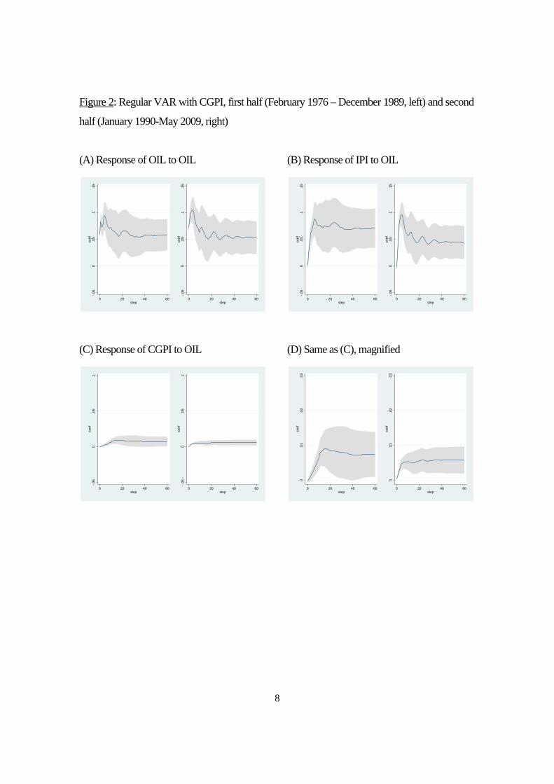
to OIL) and responses of IPI and domestic price indices. Figure 2 reports the case in which the
domestic price index is CGPI total. In all the panels reported in this section, the left hand side
figure is for the first half, and the right hand side is the second half. Also, the shaded areas are the
95 percentile bands. Panel (A) corresponds to the response of OIL to an OIL shock. Panel (B) is
the response of IPI to OIL, and (C) is the response of CGPI to OIL. Note that the scales in Panels
(B) and (C) are set in the same way as in (A) for the sake of comparison. But this makes the
graphs in (C) too small. For that reason, in Panel (D), we present the same graph as in (C) but
with a different scale. Note, first, that the sizes of the responses of OIL to an “own shock” are not
that different between the first half and the second half (Panel (A)). This means that we can study
changes in the magnitudes of pass-through primarily by looking at the responses of domestic
prices7. Panel (B) shows that, within six months to one year, changes in the world wide oil prices
are passed onto import prices to Japan, almost fully. Panel (C) shows that the response of CGPI
to OIL was small compared with the own response, even during the first half and that it declined
further in the second half (which is more evident in the magnified graphs in (D)).
7 To illustrate this point, consider the following counterfactual example: suppose that the responses of CGPI to OIL are of about the same size between the two periods, but the response of OIL to itself in the second half is twice as large as that in the first half. In such a case, it is reasonable to conclude that the pass-through rate of OIL to CGPI was halved in the second half. This example suggests importance of looking at the sizes of “own responses” in drawing economic conclusions.
8
Figure 2: Regular VAR with CGPI, first half (February 1976 – December 1989, left) and second
half (January 1990-May 2009, right)
(A) Response of OIL to OIL
-.05
0.0
5.1
.15
coirf
0 20 40 60step
-.05
0.0
5.1
.15
coirf
0 20 40 60step
(C) Response of CGPI to OIL
-.05
0.0
5.1
coirf
0 20 40 60step
-.05
0.0
5.1
coirf
0 20 40 60step
(B) Response of IPI to OIL
-.05
0.0
5.1
.15
coirf
0 20 40 60step
-.05
0.0
5.1
.15
coirf
0 20 40 60step
(D) Same as (C), magnified
0.0
1.0
2.0
3co
irf
0 20 40 60step
0.0
1.0
2.0
3co
irf
0 20 40 60step
9
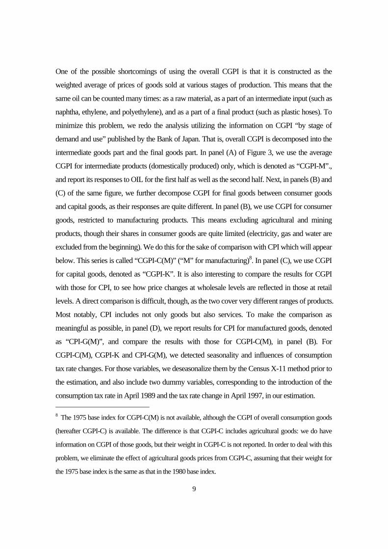
One of the possible shortcomings of using the overall CGPI is that it is constructed as the
weighted average of prices of goods sold at various stages of production. This means that the
same oil can be counted many times: as a raw material, as a part of an intermediate input (such as
naphtha, ethylene, and polyethylene), and as a part of a final product (such as plastic hoses). To
minimize this problem, we redo the analysis utilizing the information on CGPI “by stage of
demand and use” published by the Bank of Japan. That is, overall CGPI is decomposed into the
intermediate goods part and the final goods part. In panel (A) of Figure 3, we use the average
CGPI for intermediate products (domestically produced) only, which is denoted as “CGPI-M”.,
and report its responses to OIL for the first half as well as the second half. Next, in panels (B) and
(C) of the same figure, we further decompose CGPI for final goods between consumer goods
and capital goods, as their responses are quite different. In panel (B), we use CGPI for consumer
goods, restricted to manufacturing products. This means excluding agricultural and mining
products, though their shares in consumer goods are quite limited (electricity, gas and water are
excluded from the beginning). We do this for the sake of comparison with CPI which will appear
below. This series is called “CGPI-C(M)” (“M” for manufacturing)8. In panel (C), we use CGPI
for capital goods, denoted as “CGPI-K”. It is also interesting to compare the results for CGPI
with those for CPI, to see how price changes at wholesale levels are reflected in those at retail
levels. A direct comparison is difficult, though, as the two cover very different ranges of products.
Most notably, CPI includes not only goods but also services. To make the comparison as
meaningful as possible, in panel (D), we report results for CPI for manufactured goods, denoted
as “CPI-G(M)”, and compare the results with those for CGPI-C(M), in panel (B). For
CGPI-C(M), CGPI-K and CPI-G(M), we detected seasonality and influences of consumption
tax rate changes. For those variables, we deseasonalize them by the Census X-11 method prior to
the estimation, and also include two dummy variables, corresponding to the introduction of the
consumption tax rate in April 1989 and the tax rate change in April 1997, in our estimation. 8 The 1975 base index for CGPI-C(M) is not available, although the CGPI of overall consumption goods
(hereafter CGPI-C) is available. The difference is that CGPI-C includes agricultural goods: we do have
information on CGPI of those goods, but their weight in CGPI-C is not reported. In order to deal with this
problem, we eliminate the effect of agricultural goods prices from CGPI-C, assuming that their weight for
the 1975 base index is the same as that in the 1980 base index.

10
Figure 3: Regular VAR with alternative prices, first half (February 1976 – December 1989, left)
and second half (January 1990-May 2009, right)
(A) Response of CGPI-M to OIL
0.0
1.0
2.0
3co
irf
0 20 40 60step
0.0
1.0
2.0
3co
irf
0 20 40 60step
(B) Response of CGPI-C(M) to OIL (C) Response of CGPI-K to OIL
0.0
1.0
2.0
3co
irf
0 20 40 60step
0.0
1.0
2.0
3co
irf
0 20 40 60step
(D) Response of CPI-G(M) to OIL
0.0
1.0
2.0
3co
irf
0 20 40 60step
0.0
1.0
2.0
3co
irf
0 20 40 60step
0.0
1.0
2.0
3co
irf
0 20 40 60step
0.0
1.0
2.0
3co
irf
0 20 40 60step

11
Going through different panels of Figure 3, we see that the general tendency for
declining pass-through applies to those alternative measures of domestic prices as well.
We can also see that the pass-through rate tends to decline as we move downstream
from CGPI-M to CGPI-C(M) and CGPI-K, with the former being more sensitive to oil
price changes than the latter. Comparing panels (B) and (D), we can see that the
responses of CGPI-C(M) are smaller than those for CPI-G(M). The result seems quite
puzzling, because wholesale prices, which are more “upstream”, are expected to be
more sensitive to oil price changes than retail prices, which are more “downstream”. We
shall come back to this issue in the next section.
3 Evidence from TVP-VARs
3-1 Evidence for aggregate prices
As we have already argued, regular VARs with sub-samples are not necessarily helpful
in detecting timing and speed of structural changes. In this section, we employ a time
varying parameter VARs (TVP-VARs) to overcome these shortcomings. Refer to
Appendix at the end of the paper for the details of the empirical method employed here.
Very briefly, our method is an application of the Kalman Fliter, and only the reduced
form VAR coefficients are allowed to change over time.
In this section, we continue with our study on aggregate domestic prices. As in the
previous section, we estimate a series of TVP-VARs with three variables, namely OIL,
IIP, and a measure of domestic prices9. In Figure 4, we show an example in which we
use CGPI as the domestic price index. These are impulse responses, evaluated at
January of years 1980, 1985, 1990, 1995, 2000, 2005, and 2009, of each variable to an
OIL shock. We can observe that the responses of CGPI shifted upward during the 1980s,
moved down sharply at the beginning of the 1990s, and then continued to decline
gradually until the mid-2000s. There is a slight shift upward in 2009. 9 Both the VAR and the TVP-VAR approaches treat OIL as an endogenous variable. It might be more appropriate to model it as exogenous to the Japanese economy. We tried estimating a TVP-VARX model with OIL, IPI and CGPI (total), in which OIL is regarded as an exogenous variable. The estimated pass-through rates were virtually the same as the ones reported below. For this reason, in the paper, we report results from standard TVP-VARs.

12
Figure 4: TVP-VAR results for CGPI total: Impulse responses to OIL
0 5 10 15 20 25 300.02
0.04
0.06
0.08
0.1response of OIL to OIL
1980
1985
1990
1995
2000
2005
2009
0 5 10 15 20 25 30-0.05
0
0.05
0.1response of IPI to OIL
0 5 10 15 20 25 300
0.005
0.01
0.015response of CGPI to OIL
While the regular impulse responses in Figure 4 are undoubtedly informative, it is
difficult to grasp the big picture from here. This is especially so because we wish to
compare the responses of the domestic price index (CGPI here) with the “own
responses” at each point in time. Next, we try to summarize the vast information
provided by the estimation in a little more succinct way. In Figure 5, we report time
series evolution of the estimated “pass-through rates”. With respect to an OIL shock, it
is defined in the following way:
(Pass-through rate of OIL at time horizon s in period t)
= (impulse response of domestic price to an OIL shock at horizon s in period t)
/ (impulse response of OIL to an OIL shock at horizon s in period t).
We present the results in three dimensional graphs. On the vertical axis, we put the
estimated pass-through rate as defined above. On the axis titled “year”, we put time
period (we show results for January of each year). On the axis labeled “horizon”, we put
the time horizon, i.e., the number of months after the shock hits. Along the time period
dimension, we start all the figures from 1979. This is because, in the TVP-VARs, the

13
first few years of estimation results tend to be influenced by initial values set by the
researcher.
Figure 5 Estimated Pass-through rates for aggregate price indices
(A) CGPI total
05
1015
2025 1979
19841989
19941999
20042009
0
0.05
0.1
0.15
0.2
0.25
0.3
0.35
yearhorizon
pass
-th
rough
rat
e
(B) CGPI-M
05
1015
2025 1979198419891994199920042009
0
0.05
0.1
0.15
0.2
0.25
0.3
0.35
yearhorizon
pass
-th
rough
rat
e

14
(C) CGPI-C(M)
05
1015
2025
19791984
19891994
19992004
2009
0
0.05
0.1
0.15
0.2
0.25
0.3
0.35
yearhorizon
pass
-th
rough
rat
e
(D) CGPI-K
05
1015
2025
1979198419891994199920042009
0
0.05
0.1
0.15
0.2
0.25
0.3
0.35
year
pass
-th
rough
rat
e
15
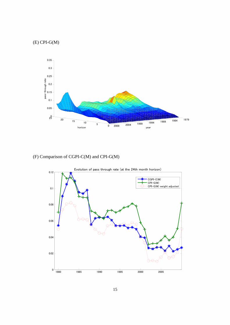
(E) CPI-G(M)
05
1015
2025
1979198419891994199920042009
0
0.05
0.1
0.15
0.2
0.25
0.3
0.35
yearhorizon
pass
-th
rough
rat
e
(F) Comparison of CGPI-C(M) and CPI-G(M)
1980 1985 1990 1995 2000 20050
0.02
0.04
0.06
0.08
0.1
0.12Evolution of pass through rate (at the 24th month horizon)
CGPI-C(M)
CPI-G(M)
CPI-G(M) weight adjusted
16
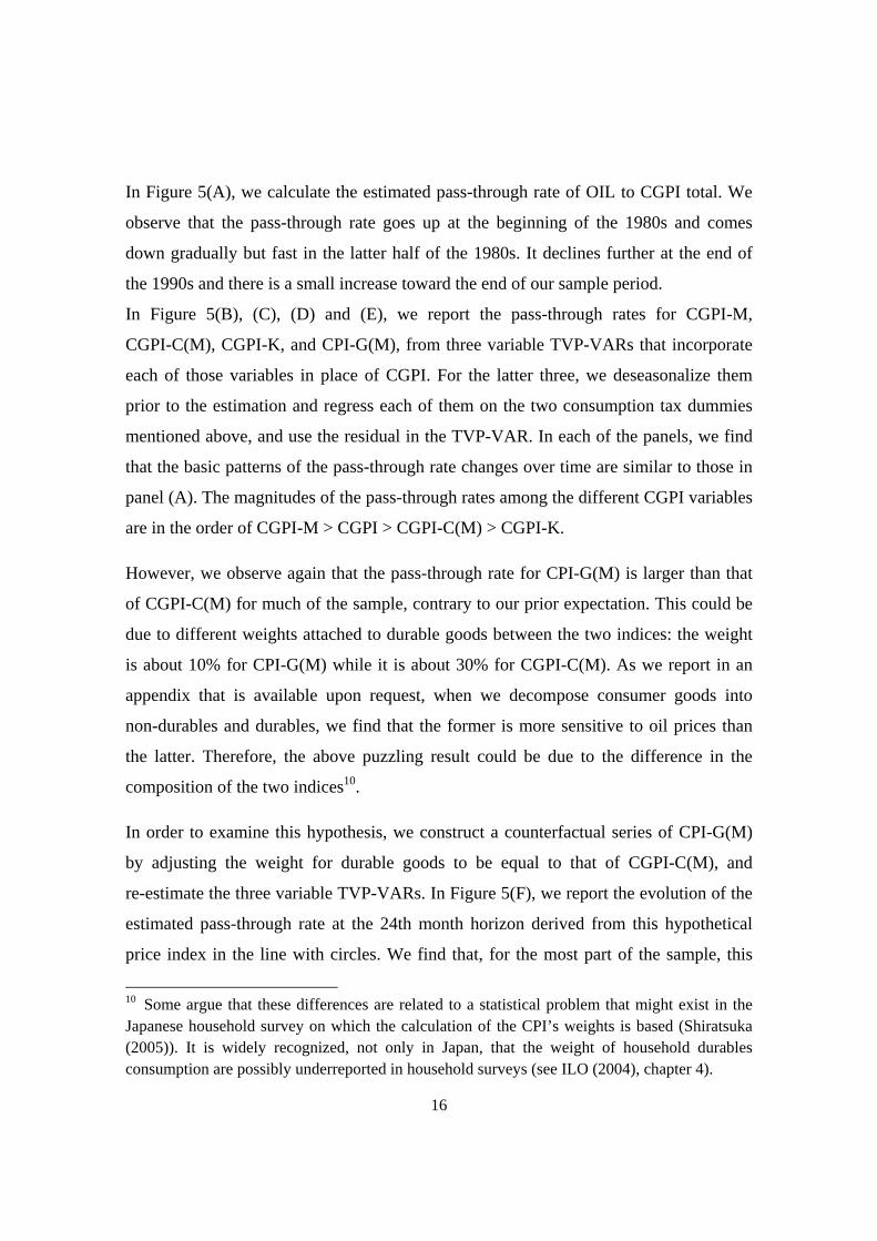
In Figure 5(A), we calculate the estimated pass-through rate of OIL to CGPI total. We
observe that the pass-through rate goes up at the beginning of the 1980s and comes
down gradually but fast in the latter half of the 1980s. It declines further at the end of
the 1990s and there is a small increase toward the end of our sample period.
In Figure 5(B), (C), (D) and (E), we report the pass-through rates for CGPI-M,
CGPI-C(M), CGPI-K, and CPI-G(M), from three variable TVP-VARs that incorporate
each of those variables in place of CGPI. For the latter three, we deseasonalize them
prior to the estimation and regress each of them on the two consumption tax dummies
mentioned above, and use the residual in the TVP-VAR. In each of the panels, we find
that the basic patterns of the pass-through rate changes over time are similar to those in
panel (A). The magnitudes of the pass-through rates among the different CGPI variables
are in the order of CGPI-M > CGPI > CGPI-C(M) > CGPI-K.
However, we observe again that the pass-through rate for CPI-G(M) is larger than that
of CGPI-C(M) for much of the sample, contrary to our prior expectation. This could be
due to different weights attached to durable goods between the two indices: the weight
is about 10% for CPI-G(M) while it is about 30% for CGPI-C(M). As we report in an
appendix that is available upon request, when we decompose consumer goods into
non-durables and durables, we find that the former is more sensitive to oil prices than
the latter. Therefore, the above puzzling result could be due to the difference in the
composition of the two indices10.
In order to examine this hypothesis, we construct a counterfactual series of CPI-G(M)
by adjusting the weight for durable goods to be equal to that of CGPI-C(M), and
re-estimate the three variable TVP-VARs. In Figure 5(F), we report the evolution of the
estimated pass-through rate at the 24th month horizon derived from this hypothetical
price index in the line with circles. We find that, for the most part of the sample, this
10 Some argue that these differences are related to a statistical problem that might exist in the Japanese household survey on which the calculation of the CPI’s weights is based (Shiratsuka (2005)). It is widely recognized, not only in Japan, that the weight of household durables consumption are possibly underreported in household surveys (see ILO (2004), chapter 4).

17
pass-through rate is lower than that for CGPI-C(M). This result is consistent with our
hypothesis11.
Although our primary interest in this paper is in variations of the pass-through rates
over time, it is also of interest to see how the levels of the pass-through rates in Japan
compare with those of other countries, especially in Asia. Jongwanich and Park (2008)
conduct VAR analyses of oil price pass-through for various countries in Asia, for the
late 1990s and the 2000s, and report their estimated pass-through rates, defined in the
same way as in our study. Their estimated rate for PPI is high for Indonesia (around
0.22), Malaysia (0.16), Singapore (0.16), and, to some extent, PRC (0.14). Korea,
Thailand, and the Philippines are intermediate cases with about 0.07. The rate is much
lower for India and Vietnam. In Figure 5(A), the pass-through rate for CGPI for the
same period varies between 0.06 and 0.12 at the 24th month horizon, which places Japan
below Indonesia, PRC, etc., and closer to Korea and Thailand. This may not be so
surprising: Japan, for an industrialized country, has had a high share of manufacturing,
especially heavy manufacturing such as automobiles. Even if each plant is energy
efficient, it is still possible that the country as a whole is rather energy intensive. Before
jumping up to a conclusion, however, we would have to further investigate
comparability of the data between Japan and those countries.
3-2 Evidence from Plastic
The previous sub-section revealed declining tendencies of pass-through of oil prices to
Japanese aggregate prices. This, however, could be due to a mixture of two causes:
declines in responsiveness of prices of oil-related products to oil prices, and increases in
the shares of non-oil-related products (and also services, in the case of CPI). To extract
the former effects from the data, we now turn our attention to industry level price data
and focus on products that are very oil intensive. In this sub-section, we take up plastic
11 Exceptions are in the latter half of the 1990s and around the year 2009. The difference in the estimated pass-through rates between the two is relatively small for the former period. The difference is larger for the last part of our sample: a possible cause is a deregulation of the retail market for gasoline: refer to the discussion in section 3-3.

18
and related products. Distilling crude oil at oil refineries produces “naphtha”, among
other things, and cracking naphtha in petrochemical steam crackers yields so-called
“basic petrochemical products” (ethylene, propylene, benzene, etc.), and they are used
to produce various types of “plastic” (polyethylene, polypropylene, etc.). Then plastic is
supplied for various purposes, including production of so-called “plastic products”
(such as plastic hoses). Here, we study how the pass-through rates of crude oil prices to
those products at each of these stages evolved over time.
Figure 6: Estimated pass-through rates for plastic and related products
(A) Naphtha (CGPI)
05
1015
2025 1979198419891994199920042009
0
0.5
1
1.5
2
2.5
yearhorizon
pass
-th
rough
rat
e
19
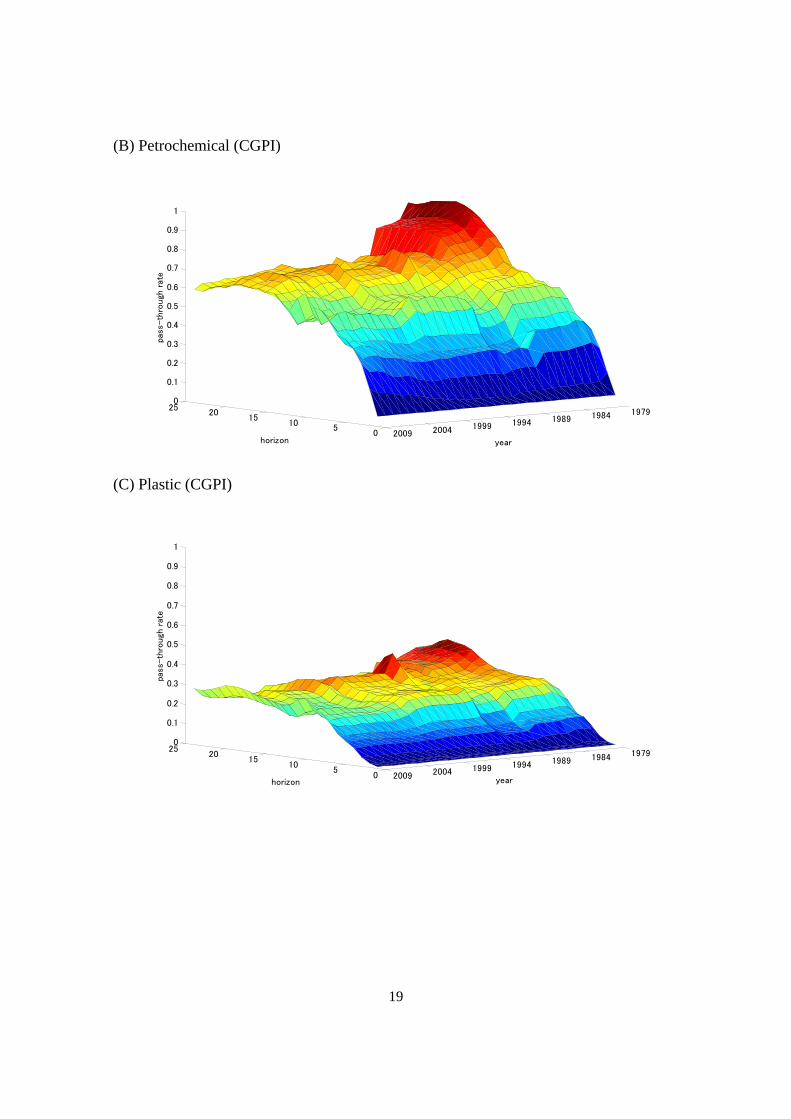
(B) Petrochemical (CGPI)
05
1015
2025 1979198419891994199920042009
0
0.1
0.2
0.3
0.4
0.5
0.6
0.7
0.8
0.9
1
yearhorizon
pass
-th
rough
rat
e
(C) Plastic (CGPI)
05
1015
2025 1979198419891994199920042009
0
0.1
0.2
0.3
0.4
0.5
0.6
0.7
0.8
0.9
1
yearhorizon
pass
-th
rough
rat
e
20
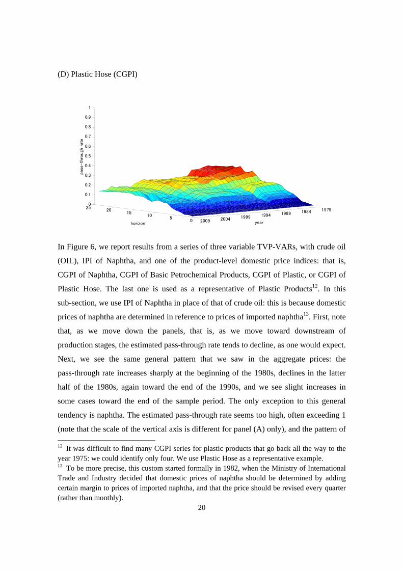
(D) Plastic Hose (CGPI)
05
1015
2025 1979198419891994199920042009
0
0.1
0.2
0.3
0.4
0.5
0.6
0.7
0.8
0.9
1
yearhorizon
pass
-th
rough
rat
e
In Figure 6, we report results from a series of three variable TVP-VARs, with crude oil
(OIL), IPI of Naphtha, and one of the product-level domestic price indices: that is,
CGPI of Naphtha, CGPI of Basic Petrochemical Products, CGPI of Plastic, or CGPI of
Plastic Hose. The last one is used as a representative of Plastic Products12. In this
sub-section, we use IPI of Naphtha in place of that of crude oil: this is because domestic
prices of naphtha are determined in reference to prices of imported naphtha13. First, note
that, as we move down the panels, that is, as we move toward downstream of
production stages, the estimated pass-through rate tends to decline, as one would expect.
Next, we see the same general pattern that we saw in the aggregate prices: the
pass-through rate increases sharply at the beginning of the 1980s, declines in the latter
half of the 1980s, again toward the end of the 1990s, and we see slight increases in
some cases toward the end of the sample period. The only exception to this general
tendency is naphtha. The estimated pass-through rate seems too high, often exceeding 1
(note that the scale of the vertical axis is different for panel (A) only), and the pattern of 12 It was difficult to find many CGPI series for plastic products that go back all the way to the year 1975: we could identify only four. We use Plastic Hose as a representative example. 13 To be more precise, this custom started formally in 1982, when the Ministry of International Trade and Industry decided that domestic prices of naphtha should be determined by adding certain margin to prices of imported naphtha, and that the price should be revised every quarter (rather than monthly).

21
the time variation is unclear. This could be because, as mentioned above, prices of
domestically produced naphtha are determined by some non-market rule.
3-3 Evidence from Gasoline
Next, we turn to the case of gasoline. Again, we estimate a three variables TVP-VAR,
with OIL, IPI of crude oil, and CPI of gasoline. To control for disruptive effects of a
temporary reduction and a subsequent increase in the gasoline tax rate in 2008, we first
regress log differences of gasoline prices on the March 2008 dummy and the April 2008
dummy. Then the residuals are included in out TVP-VAR estimation. We report the
estimated pass-through rates in Figure 7(A). We observe that the level of the
pass-through rate is lower compared with, for example, naphtha. Its tendency to decline
over time, before starting to increase again in the late 2000s, is similar to the previous
results.
Figure 7: (A) Estimated pass-through rate for Gasoline (CPI)
05
1015
2025
19791984
19891994
19992004
2009
0
0.1
0.2
0.3
0.4
0.5
0.6
0.7
0.8
0.9
1
yearhorizon
pass
-th
rough
rat
e
22
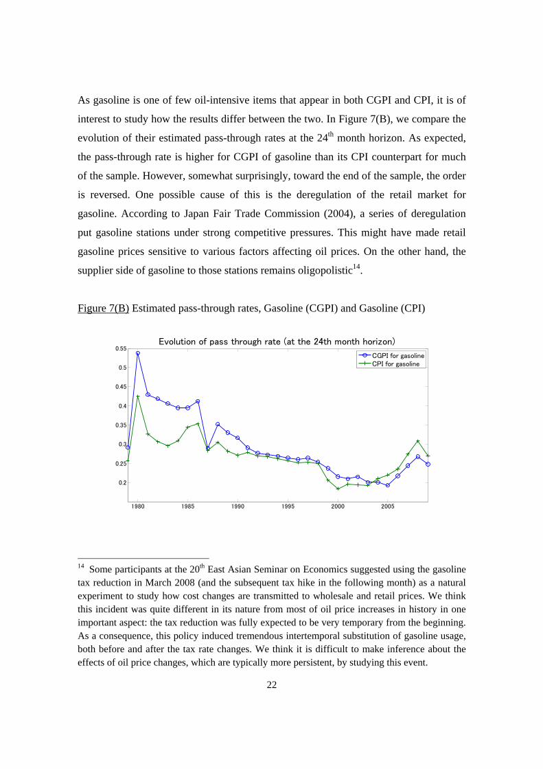
As gasoline is one of few oil-intensive items that appear in both CGPI and CPI, it is of
interest to study how the results differ between the two. In Figure 7(B), we compare the
evolution of their estimated pass-through rates at the 24th month horizon. As expected,
the pass-through rate is higher for CGPI of gasoline than its CPI counterpart for much
of the sample. However, somewhat surprisingly, toward the end of the sample, the order
is reversed. One possible cause of this is the deregulation of the retail market for
gasoline. According to Japan Fair Trade Commission (2004), a series of deregulation
put gasoline stations under strong competitive pressures. This might have made retail
gasoline prices sensitive to various factors affecting oil prices. On the other hand, the
supplier side of gasoline to those stations remains oligopolistic14.
Figure 7(B) Estimated pass-through rates, Gasoline (CGPI) and Gasoline (CPI)
1980 1985 1990 1995 2000 2005
0.2
0.25
0.3
0.35
0.4
0.45
0.5
0.55Evolution of pass through rate (at the 24th month horizon)
CGPI for gasolineCPI for gasoline
14 Some participants at the 20th East Asian Seminar on Economics suggested using the gasoline tax reduction in March 2008 (and the subsequent tax hike in the following month) as a natural experiment to study how cost changes are transmitted to wholesale and retail prices. We think this incident was quite different in its nature from most of oil price increases in history in one important aspect: the tax reduction was fully expected to be very temporary from the beginning. As a consequence, this policy induced tremendous intertemporal substitution of gasoline usage, both before and after the tax rate changes. We think it is difficult to make inference about the effects of oil price changes, which are typically more persistent, by studying this event.

23
3-4 Evidence from Electricity
Finally, we turn to the case of electricity. In this case, we estimate a three variable
TVP-VAR, with OIL, IPI of “crude oil, coal and natural gas”, and CGPI of electric
power. We include natural gas etc. in our definition of IPI here, because even thermal
power plants use not only oil but also coal and natural gas15. CGPI of electric power is
deseasonalized by the Census X-11 Method. We report the estimated pass-through rates
in Figure 8. We can observe continuous declines in the pass-through rate, starting in the
early 1980s and lasting throughout much of the sample period, until it starts to increase
again toward the end of the sample.
Figure 8: Estimated pass-through rate for Electricity
05
1015
2025 1979198419891994199920042009
-0.1
0
0.1
0.2
0.3
0.4
0.5
0.6
0.7
yearhorizon
pass
-th
rough
rat
e
To summarize this section, we have seen that the declines in the pass-through rates at
the aggregate level are not simply a result of shrinking shares of oil-related products.
Even at the level of those products, we can find declines in the pass-through rates. In the
next section, we study implications from the Input-Output Tables to see if this can be
explained from changes in the cost structure of oil-related production.
15 In fact, oil has come to play a relatively minor role. We shall discuss this matter further in the next section.

24
4 Cost structure and pass-through rates: what do the Input-Output
Tables predict? The 1980-2000 period.
4-1 Data and Methodology
In Japan, frequent changes in rules and methodology (such as classification of goods
and services) make a long run comparison of input-output structure difficult.
Fortunately, the Research Institute for Economy, Trade and Industry (RIETI) provide
detailed Input-Output Tables for years 1980, 1985, 1990, 1995 and 2000 that are
directly comparable between each other. They provide tables in both nominal units and
real (constant 1995 price) units. Each of the tables contains 511 rows (industries that
provide inputs) and 398 columns (industries that use those inputs). Most notably, “crude
oil” appears as a single row item (though, on the column side, it is combined with
natural gas). Also, different types of Petroleum Products, such as “gasoline”, “naphtha”,
“fuel oil A” and “fuel oil B&C”, all appear as separate items on the row side (though
they are all combined into one on the column side). This is important, as different types
of Petroleum Products receive very different tax treatments. We make suitable
assumptions to expand the tables into matrices of dimensions 511 times 51116.
Naturally, we are also interested in the period after 2000. The next section employs
more recent I-O tables, which are much smaller than the ones explained above (due to
limited data availability), to study the 2000s.
16 The numbers of columns and rows do not coincide basically because certain row industries are combined into single column industries. In such cases, in principle, we assume that each row industry that belongs to the same column industry group has the same input structure. There are only very minor exceptions in which the correspondence between the row industries and the column industries is not perfect. For Petroleum Products, it is important to consider the fact that different types of products are subject to very different tax schemes. For this reason, we take the following approach. From the input-output table for each year, we obtain the total amount of indirect taxes paid by the whole Petroleum Products sector. From tax revenue statistics of the Ministry of Finance, we obtain the shares of taxes imposed on each type of Petroleum Products. We allocate indirect taxes to each of the sub-sectors according to those shares. The rest of the cost structure is assumed to be the same across those sub-sectors. We consider this to be a reasonable assumption, as all of those products are by-products of a single distillation process.

25
The I-O Tables can be used to derive predictions on a percentage response of the
average price of products of a certain sector when the price of imported goods (say) of
another sector increases by 1%. The Input-Output analysis with N sectors (with trade)
has the following basic structure:
( )x Ax d e M Ax d
where x is the vector of output ( 1N ), A is the input coefficient matrix, d is the vector
of domestic final demand ( 1N ), e is the vector of exports ( 1N ), and M is the matrix
of import coefficients. The matrix M is a diagonal matrix whose ith diagonal element is
the ratio of the imports of the ith sector to the sum of intermediate inputs from the ith
sector to all the sectors plus the domestic final demand to this sector’s output. From
here, it is possible to derive the following pricing equation:
1' ' ' mp I I M A A M p
,
where p is the vector of the rate of domestic price change in each sector and mp is
the vector of the rate of price change of imported goods in each sector. For example,
suppose that the crude oil sector is the Jth sector and that we wish to study the impact of
one percentage increase in imported crude oil price. Then we set the Jth element of the
vector mp to be 1 and all the other elements to be 0. Then each element of p
would indicate the predicted percentage increase in the domestic prices of goods in each
sector, under the assumption of flexible prices (complete pass-through at each
production stage) and zero substitution. In essence, the above equation provides a way
to compute “oil contents” of the cost of production for each sector, which takes into
account the complex input output structure of the economy.
In this paper, we utilize both nominal and real I-O tables to derive those predictions.
The current prices table will predict the impact of an increase in oil prices given the
current cost structure of each industry. The constant price table, on the other hand, will
give a hypothetical prediction on what would happen if only the real cost structure
changed between the current year and the bench-mark year (due to, for example,
substitution between oil and other types of materials) while maintaining the same
26
relative price structure. It turns out that differences in predictions from those two types
of tables are quite informative.
4-2 Plastic, 1980-2000
We start with product level analysis here. Figure 9(A) uses the nominal I-O Tables to
derive the predicted responses of Naphtha, Basic Petrochemical Products (ethylene,
propylene, benzene, etc.), Thermoplastic Resin (a type of plastic: polyethylene,
polypropylene, etc.), and Plastic Products. Solid lines with cubes show the predicted
percentage responses of those prices when the price of imported crude oil increases by
one percent. Dashed lines with triangles show the predicted responses when imported
prices of both crude oil and petroleum products increase by one percent, simultaneously.
This calculation is necessary because currently Japan imports much of naphtha it needs
from abroad (which was not the case in 1980). Solid lines with circles show what
happens when prices of all the imported goods increase simultaneously by one percent.
Figure 9(B) performs an analogous study using the real I-O Tables (1995 constant
prices).
The contrast between Figure 9(A) and 9(B) is striking. While the nominal I-O Table
predicts sharp declines in the price responsiveness over time, the real I-O Table does not
predict any systematic tendency. The fact that the real I-O table does not predict much
decline suggests that there was not much of a real substitution away from the use of oil
during this period. We had expected a decline in the importance of oil, at the very least
in the comparative sense, as we had originally thought the importance of services such
as distribution and finance would have increased over time: apparently, that did not
happen. Yet the nominal I-O table tells a very different story. The difference comes
from the fact that, during this period, there were substantial declines in prices of
imported oil, naphtha, and other imports. To summarize, although there were very little
substitution between quantities of different types of input, the relative importance of oil
still declined substantially basically because it became cheaper. As the lower price of oil
reduced its share in overall nominal production costs, prices of those products became
much less responsive to fluctuations in oil prices.

27
Figure 9: Predicted responses of Plastic and related products to OIL etc.
(A) Predictions from NOMINAL I-O Tables
1980 1985 1990 1995 20000
0.1
0.2
0.3
0.4
0.5
0.6
0.7
0.8
0.9
1Naphtha
Crude Oil
Crude Oil + Pet ProductsOverall Imports
1980 1985 1990 1995 20000
0.1
0.2
0.3
0.4
0.5
0.6
0.7
0.8
0.9
1Basic Petrochemical Products (Ethylene etc.)
Crude Oil
Crude Oil + Pet ProductsOverall Imports
1980 1985 1990 1995 20000
0.1
0.2
0.3
0.4
0.5
0.6
0.7
0.8
0.9
1Thermoplastic Resin (Polyethylene etc.)
Crude Oil
Crude Oil + Pet ProductsOverall Imports
1980 1985 1990 1995 20000
0.1
0.2
0.3
0.4
0.5
0.6
0.7
0.8
0.9
1Plastic Products
Crude Oil
Crude Oil + Pet ProductsOverall Imports
(B) Predictions from REAL I-O Tables (1995 constant prices)
1980 1985 1990 1995 20000
0.1
0.2
0.3
0.4
0.5
0.6
0.7
0.8
0.9
1Naphtha
Crude Oil
Crude Oil + Pet ProductsOverall Imports
1980 1985 1990 1995 20000
0.1
0.2
0.3
0.4
0.5
0.6
0.7
0.8
0.9
1Basic Petrochemical Products (Ethylene etc.)
Crude Oil
Crude Oil + Pet ProductsOverall Imports
1980 1985 1990 1995 20000
0.1
0.2
0.3
0.4
0.5
0.6
0.7
0.8
0.9
1Thermoplastic Resin (Polyethylene etc.)
Crude Oil
Crude Oil + Pet ProductsOverall Imports
1980 1985 1990 1995 20000
0.1
0.2
0.3
0.4
0.5
0.6
0.7
0.8
0.9
1Plastic Products
Crude Oil
Crude Oil + Pet ProductsOverall Imports

28
How do these predictions in Figure 9(A) compare with the actual estimation results in
Figure 6? Comparing the two panel by panel (looking at the long run estimated
pass-through rates at the 24 months horizon in each panel of Figure 6), we learn that the
cost-related factors that appear in Figure 9(A) are enough (in some cases, more than
enough) to explain the declines in the estimated pass-through rates. Our conclusion for
these sectors is that the pass-through rates of oil declined because oil became cheaper
and thus became less important in overall costs for those sectors.
4-3 Gasoline, 1980-2000
Studying the case of gasoline in Japan requires a caution, as it is subject to heavy
taxation17. What is important is that those taxes are per-unit taxes (or specific duties) as
opposed to ad valorem taxes. Taxes therefore do not go up when oil prices increase. In
the period of high oil prices, the share of those taxes in overall gasoline prices is thus
relatively low. Gasoline prices will move nearly one-for-one with oil prices. When oil
prices are lower, the share of taxes, the portion that does not respond to oil price
fluctuations, in overall gasoline prices is higher. Gasoline prices are thus expected to be
less responsive to oil price changes. Pass-through rates of oil prices are thus expected to
change endogenously with the level of oil prices. This could at least partially explain the
declining pass-through rate we saw in Figure 7.
In fact, we estimate that, as of 1980, indirect taxes were equal to about 29.6% of total
output value of gasoline. In 2000, this ratio was up to as high as 53.8%.
To study the magnitude of this effect, in Figure 10(A), we first compute predicted
response of gasoline prices to oil prices from the nominal I-O tables, under the actual
cost structure (solid line with cubes). Note that those predictions are fairly close to the
actual estimated pass-through rates, that are reported in Figure 7, for the medium and
long runs. Next, we redo the calculation under the counterfactual assumption that the
indirect taxes did not exist (or the taxes move proportionately with prices), and the
results appear in dashed line with triangles. Lastly, we redo the analysis by assuming 17 Also, diesel and jet fuel are heavily taxed in Japan. On the other hand, naphtha and heavy fuel oil are, relatively speaking, lightly taxed. This necessitates careful treatment of indirect taxes that we explained in the previous section.
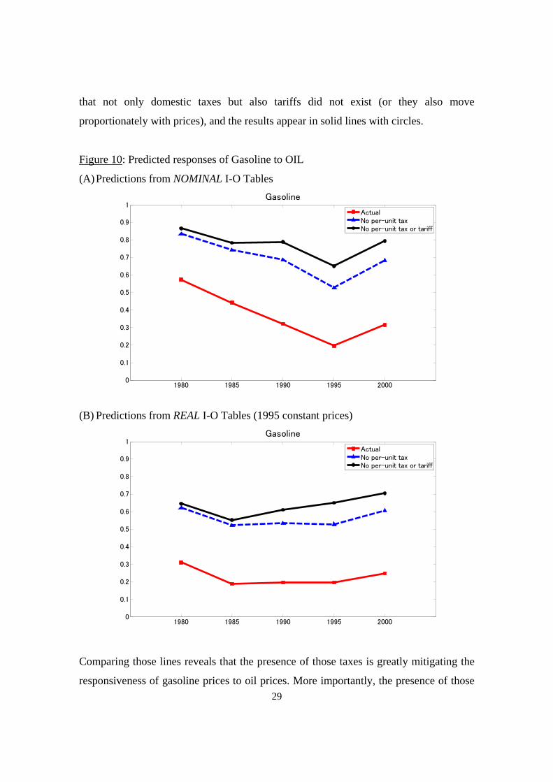
29
that not only domestic taxes but also tariffs did not exist (or they also move
proportionately with prices), and the results appear in solid lines with circles.
Figure 10: Predicted responses of Gasoline to OIL
(A) Predictions from NOMINAL I-O Tables
1980 1985 1990 1995 20000
0.1
0.2
0.3
0.4
0.5
0.6
0.7
0.8
0.9
1Gasoline
ActualNo per-unit taxNo per-unit tax or tariff
(B) Predictions from REAL I-O Tables (1995 constant prices)
1980 1985 1990 1995 20000
0.1
0.2
0.3
0.4
0.5
0.6
0.7
0.8
0.9
1Gasoline
ActualNo per-unit taxNo per-unit tax or tariff
Comparing those lines reveals that the presence of those taxes is greatly mitigating the
responsiveness of gasoline prices to oil prices. More importantly, the presence of those
30
taxes made the responsiveness to decline substantially between 1980 and 2000. Without
those taxes and tariffs, the responsiveness would have decreased by relatively small
percentages. Figure 10(B) does analogous calculation based on the real I-O table. We
see that, without the effects of nominal price levels and taxes and tariffs, the
responsiveness would have remained nearly constant, and high. We conclude that the
declining pass-through rates in Figure 7 could possibly be explained entirely by those
two effects.
4-4 More on the importance of taxes: Diesel and “Type A fuel”, 1980-2000
To further investigate the importance of the presence of taxes in pass-through of oil
prices, we next consider two types of petroleum products, diesel and so-called “type A
fuel”. Those two are almost identical in their physical nature. The difference is that
diesel is heavily taxed. From the I-O tables, we estimate that the ratio of indirect taxes
to diesel production was 20.0% for 1980 and 40.6% in 2000. On the other hand, type A
fuel is very lightly taxed. As a consequence, usage of this type of fuel is restricted
mainly to agriculture and fishery. According to our argument in the previous
sub-section, we should observe higher pass-through rates for type A fuel.
In Figure 11(A), we show the difference between prices of those two types of products
(in logarithms), along with crude oil prices. It is evident that the two are highly
correlated. This is an indication that type A fuel responds more strongly to fluctuations
in oil prices, that is, their pass-through rates are higher.
Next, we estimate regular three variable VARs with OIL, IPI (of crude oil) , and either
type A fuel or diesel. Figure 11(B) shows impulse responses of type A fuel (solid line)
and diesel (dashed line) to OIL for the first half of the sample (left panels) and the
second half (right panels). We confirm our hypothesis that, as type A fuel is lightly
taxed, it tends to be more responsive to oil price changes.

31
Figure 11(A) Evolution of price differentials between type A fuel and diesel (solid line)
and oil prices (dashed line), all the prices are in logs
23
45
ln(O
IL)
-.15
-.1
-.05
0.0
5ln
(Typ
e A
Oil)
-ln(
Die
sel)
1975m1 1980m1 1985m1 1990m1 1995m1 2000m1 2005m1 2010m1Year
ln(Type A Oil)-ln(Diesel) ln(OIL)
Figure 11(B) Impulse responses to OIL of type A fuel (solid lines) and diesel (dashed
lines), first half (left) and second half (right)
0.0
2.0
4.0
6.0
8
0 20 40 60step
0.0
2.0
4.0
6.0
8
0 20 40 60step

32
4-5 Electricity, 1980-2000
We next turn to the case of electricity. There are two electricity-related entries in the I-O
table, namely electricity for business uses and self uses. We derive the predicted
responses for both of them, and the results are shown in Figure 12(A) for the nominal
table and Figure 12(B) for the real table. We study the case in which only crude oil
prices increase (solid lines with cubes), the case in which oil and natural gas prices
increase simultaneously by one percent (dashed lines with triangles) and the case in
which prices of all the imported goods increase at the same time (solid lines with
circles). The nominal tables predict substantial declines in pass-through rates of oil. The
estimated pass-through rates in Figure 8 are close to predictions that appear in the solid
line with circles in the electricity for self use case. What is noteworthy about this sector
is that, even in the predictions from the real tables, we observe some declines in the
predicted responsiveness, though the declines are much smaller compared with the
predictions from the nominal tables. The decline is most evident for “crude oil” in the
“electricity for self use” case. It is also likely that increasing use of imported coal and
construction of nuclear power plants have contributed to the general tendency.
Evidently, some part of this decline, since 1990, is the emergence of natural gas as an
alternative to using oil. Hence, we conclude that, for this sector, real substitution played
a minor but non-negligible role.
Another feature of the electricity industry is that prices were under strict regulations
previously, but a series of deregulation took place during our sample period. This would
have contributed to increase the pass-through rate. But such an increase does not seem
to show up in a noticeable manner either in Figure 8 or in 12

33
Figure 12: Predicted responses of Electricity to OIL etc.
(A) Predictions from NOMINAL I-O Tables
1980 1985 1990 1995 20000
0.1
0.2
0.3
0.4
0.5
0.6
0.7
0.8
0.9
1Electricity for business use
Crude OilCrude Oil + Nat GasOverall Imports
1980 1985 1990 1995 20000
0.1
0.2
0.3
0.4
0.5
0.6
0.7
0.8
0.9
1Electricity for self use
Crude OilCrude Oil + Nat GasOverall Imports
(B) Predictions from REAL I-O Tables (1995 constant prices)
1980 1985 1990 1995 20000
0.1
0.2
0.3
0.4
0.5
0.6
0.7
0.8
0.9
1Electricity for business use
Crude OilCrude Oil + Nat GasOverall Imports
1980 1985 1990 1995 20000
0.1
0.2
0.3
0.4
0.5
0.6
0.7
0.8
0.9
1Electricity for self use
Crude OilCrude Oil + Nat GasOverall Imports
34
4-5 Overall consumer goods prices, 1980-2000
Through the I-O analysis in this section, we have found some important elements that
could explain declining pass-through of oil prices. The most notable factor has been the
relative price factor, or the relative price of oil itself. Input substitution showed up as a
minor (but non-negligible) factor for electricity. Also, the analysis for gasoline has
pointed out importance of the tax structure. Are they important in accounting for
declines in pass-through rates in overall prices as well? To answer this question, we
apply the same procedure we have employed so far to all the sectors in manufacturing
simultaneously. Then we take weighted averages of their predicted responses, where the
weights are based on the amount consumed by households. This is an effort to derive
predictions about how manufactured consumer goods prices, or CGPI-C(M), would
respond to oil prices. The results are in Figure 13. Panel (A) uses the nominal tables.
Panel (B) uses the real tables. Panel (C) uses the nominal tables, under the hypothetical
assumption that there are no per-unit taxes or tariffs on Petroleum Products (such as
gasoline, diesel, and jet fuel).
Predictions from Panel (A) fit very well with the evolution of the estimated
pass-through rates for CGPI-C(M), that appears in Figure 5(A). This leads us to suspect
that changing cost structure could go a long way toward explaining observed declines in
pass-through between 1980 and 2000. Comparison between Panels (A) and (B), on the
other hand, seems to indicate that the real side story plays only a minor role in the
structural change that lowered pass-through during this period: we observe only slight
declines in the predicted responsiveness to imported oil, petroleum products (basically
naphtha), and natural gas. This indicates that, once again, the main factor behind the
change was the relative price factor: as oil became cheaper, it became less relevant in
the cost structure.

35
Figure 13: Predicted responses of manufactured consumer goods prices to OIL etc.
(A) Predictions from NOMINAL I-O Tables
1980 1985 1990 1995 20000
0.05
0.1
0.15
0.2
0.25
Consumer Goods (Manufacturing only)
Crude OilCrude Oil + Pet ProductsCrude Oil + Nat GasOverall Imports
(B) Predictions from REAL I-O Tables
1980 1985 1990 1995 20000
0.05
0.1
0.15
0.2
0.25
Consumer Goods (Manufacturing only)
Crude OilCrude Oil + Pet ProductsCrude Oil + Nat GasOverall Imports
(C) Predictions from NOMINAL I-O Tables with no taxes or tariffs on petroleum
products
1980 1985 1990 1995 20000
0.05
0.1
0.15
0.2
0.25
Consumer Goods (Manufacturing only)
Crude OilCrude Oil + Pet ProductsCrude Oil + Nat GasOverall Imports

36
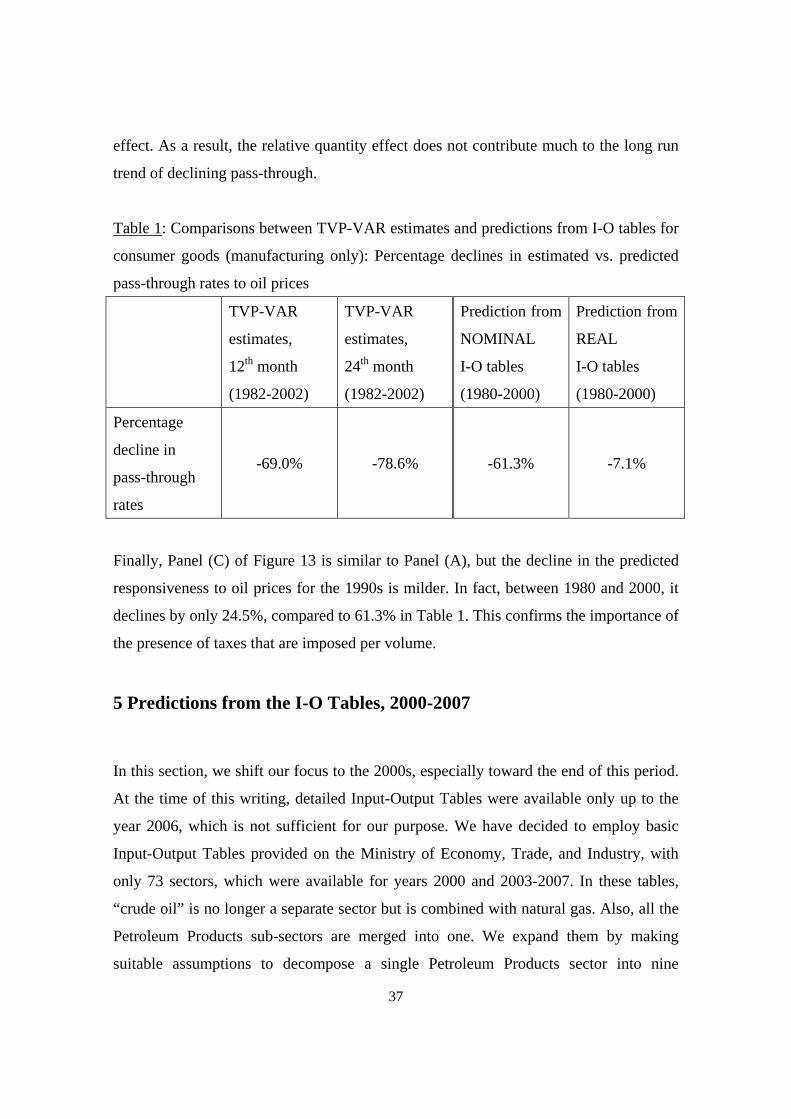
To give more formal and quantitative support to the above-mentioned impressions, in
Table 1, we contrast our TVP-VAR estimates for the pass-through rates for CGPI-C(M),
that appear in Figure 5(C), with predictions from both nominal and real I-O tables for
manufactured consumer goods, that appear in Figure 13(A) and (B). All the numbers are
percentage declines in pass-through rates, either estimated or predicted. The first
column indicates that the estimated pass-through rate at the 12th month horizon declined,
between January 1982 (its peak in Figure 5(C)) and 2002 (its bottom), by 69%.
Likewise, the second column indicates that the estimates at the 24th month horizon
declined by 78.6%. The third column indicates that the predicted pass-through rate from
the nominal I-O table declined, between 1980 and 2000, by 61.3%. Hence, changes in
cost structure, namely the relative price changes and relative quantity changes combined,
can account for between 78% and 89% of the declines in the estimated pass-through rate,
leaving only about 11% to 22% for the other factors to explain. The fourth column
indicates that the predicted pass-through rate from the real I-O table declined by just
7.1%. Thus, the relative quantity factor played a minor role in this long term decline in
the pass-through rate.
We should acknowledge that our results do not eliminate the possibility that there was
some other important factor that contributed to the declining pass-through, whose effect
was largely offset by yet another factor that happened to work in the opposite direction.
But, to be able to support such a view, one would first have to specify what this force
that was working in the other direction was, and this is, in our view, not an easy task.
It is also important to note that our results do not entirely deny the importance of the
real factor or the relative quantity factor. We have already seen that it was quite
important in the electricity sector. Figure 13(B) indicates that the relative quantity factor
was also important in the period 1980-1985: during this short period, the predicted
pass-through rate from the real I-O table declines by as much as 40.7%, and this
accounts for all of decline in the prediction from the nominal I-O table. This suggests
that, in reaction to the sudden increase in oil prices in the early 1980s, Japanese
households and firms shifted away from oil-intensive products and inputs, temporarily.
After oil prices declined in the late 1980s, however, there was some unwinding of this
37
effect. As a result, the relative quantity effect does not contribute much to the long run
trend of declining pass-through.
Table 1: Comparisons between TVP-VAR estimates and predictions from I-O tables for
consumer goods (manufacturing only): Percentage declines in estimated vs. predicted
pass-through rates to oil prices
TVP-VAR
estimates,
12th month
(1982-2002)
TVP-VAR
estimates,
24th month
(1982-2002)
Prediction from
NOMINAL
I-O tables
(1980-2000)
Prediction from
REAL
I-O tables
(1980-2000)
Percentage
decline in
pass-through
rates
-69.0% -78.6% -61.3% -7.1%
Finally, Panel (C) of Figure 13 is similar to Panel (A), but the decline in the predicted
responsiveness to oil prices for the 1990s is milder. In fact, between 1980 and 2000, it
declines by only 24.5%, compared to 61.3% in Table 1. This confirms the importance of
the presence of taxes that are imposed per volume.
5 Predictions from the I-O Tables, 2000-2007
In this section, we shift our focus to the 2000s, especially toward the end of this period.
At the time of this writing, detailed Input-Output Tables were available only up to the
year 2006, which is not sufficient for our purpose. We have decided to employ basic
Input-Output Tables provided on the Ministry of Economy, Trade, and Industry, with
only 73 sectors, which were available for years 2000 and 2003-2007. In these tables,
“crude oil” is no longer a separate sector but is combined with natural gas. Also, all the
Petroleum Products sub-sectors are merged into one. We expand them by making
suitable assumptions to decompose a single Petroleum Products sector into nine
38
sub-sectors18. As in the previous section, we compute predicted responsiveness of
sectoral prices to prices of imported oil and natural gas.
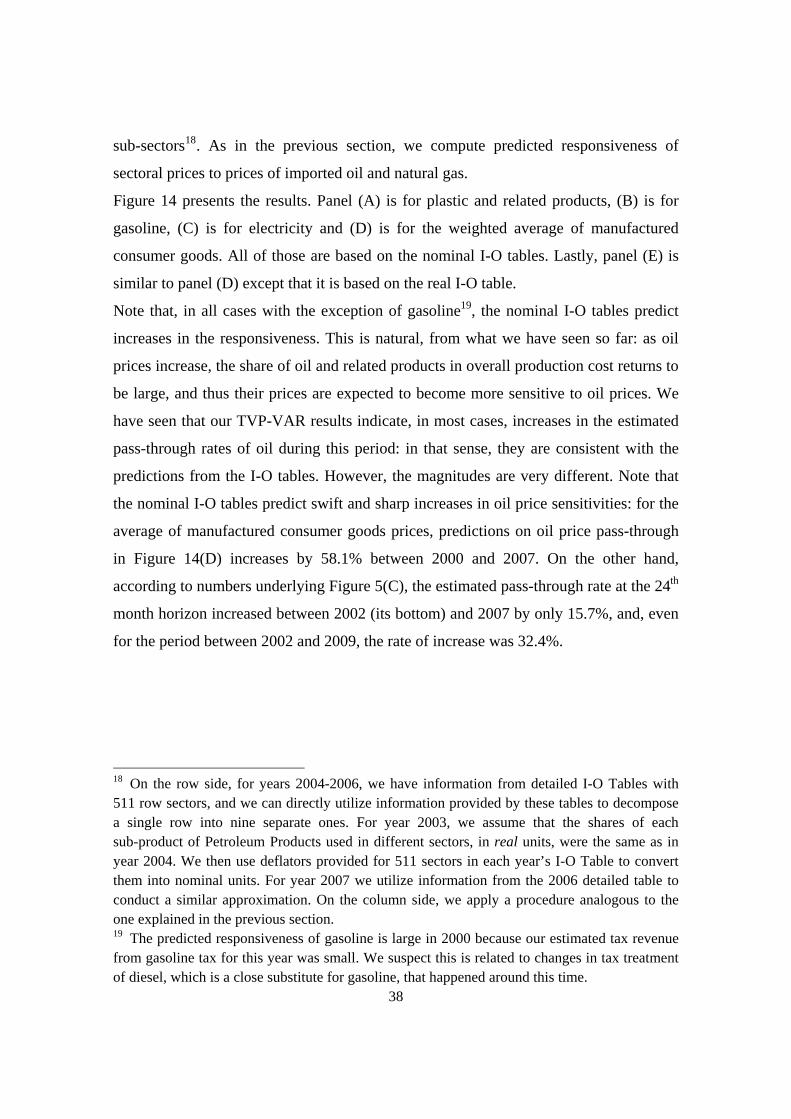
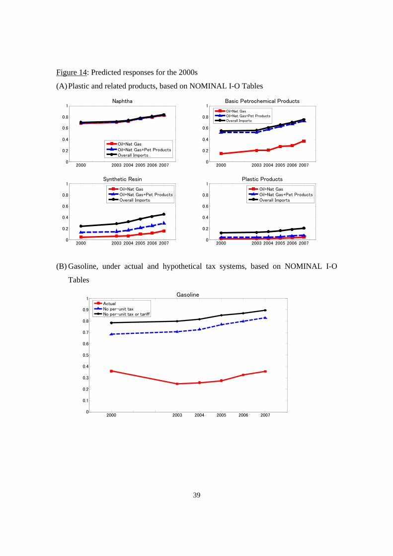
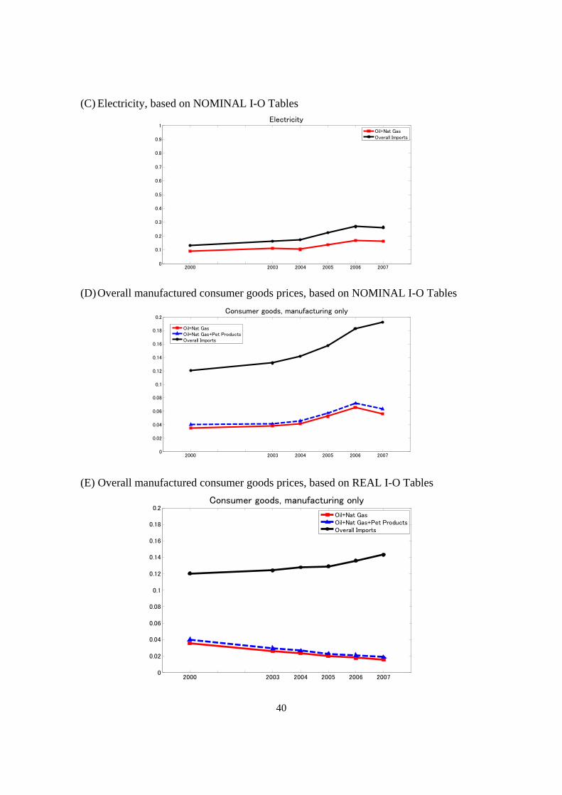
Figure 14 presents the results. Panel (A) is for plastic and related products, (B) is for
gasoline, (C) is for electricity and (D) is for the weighted average of manufactured
consumer goods. All of those are based on the nominal I-O tables. Lastly, panel (E) is
similar to panel (D) except that it is based on the real I-O table.
Note that, in all cases with the exception of gasoline19, the nominal I-O tables predict
increases in the responsiveness. This is natural, from what we have seen so far: as oil
prices increase, the share of oil and related products in overall production cost returns to
be large, and thus their prices are expected to become more sensitive to oil prices. We
have seen that our TVP-VAR results indicate, in most cases, increases in the estimated
pass-through rates of oil during this period: in that sense, they are consistent with the
predictions from the I-O tables. However, the magnitudes are very different. Note that
the nominal I-O tables predict swift and sharp increases in oil price sensitivities: for the
average of manufactured consumer goods prices, predictions on oil price pass-through
in Figure 14(D) increases by 58.1% between 2000 and 2007. On the other hand,
according to numbers underlying Figure 5(C), the estimated pass-through rate at the 24th
month horizon increased between 2002 (its bottom) and 2007 by only 15.7%, and, even
for the period between 2002 and 2009, the rate of increase was 32.4%.
18 On the row side, for years 2004-2006, we have information from detailed I-O Tables with 511 row sectors, and we can directly utilize information provided by these tables to decompose a single row into nine separate ones. For year 2003, we assume that the shares of each sub-product of Petroleum Products used in different sectors, in real units, were the same as in year 2004. We then use deflators provided for 511 sectors in each year’s I-O Table to convert them into nominal units. For year 2007 we utilize information from the 2006 detailed table to conduct a similar approximation. On the column side, we apply a procedure analogous to the one explained in the previous section. 19 The predicted responsiveness of gasoline is large in 2000 because our estimated tax revenue from gasoline tax for this year was small. We suspect this is related to changes in tax treatment of diesel, which is a close substitute for gasoline, that happened around this time.
39
Figure 14: Predicted responses for the 2000s
(A) Plastic and related products, based on NOMINAL I-O Tables
2000 2003 2004 2005 2006 20070
0.2
0.4
0.6
0.8
1Naphtha
Oil+Nat GasOil+Nat Gas+Pet ProductsOverall Imports
2000 2003 2004 2005 2006 20070
0.2
0.4
0.6
0.8
1Basic Petrochemical Products
Oil+Nat GasOil+Nat Gas+Pet ProductsOverall Imports
2000 2003 2004 2005 2006 20070
0.2
0.4
0.6
0.8
1Synthetic Resin
Oil+Nat GasOil+Nat Gas+Pet ProductsOverall Imports
2000 2003 2004 2005 2006 20070
0.2
0.4
0.6
0.8
1Plastic Products
Oil+Nat GasOil+Nat Gas+Pet ProductsOverall Imports
(B) Gasoline, under actual and hypothetical tax systems, based on NOMINAL I-O
Tables
2000 2003 2004 2005 2006 20070
0.1
0.2
0.3
0.4
0.5
0.6
0.7
0.8
0.9
1Gasoline
ActualNo per-unit taxNo per-unit tax or tariff
40
(C) Electricity, based on NOMINAL I-O Tables
2000 2003 2004 2005 2006 20070
0.1
0.2
0.3
0.4
0.5
0.6
0.7
0.8
0.9
1Electricity
Oil+Nat GasOverall Imports
(D) Overall manufactured consumer goods prices, based on NOMINAL I-O Tables
2000 2003 2004 2005 2006 20070
0.02
0.04
0.06
0.08
0.1
0.12
0.14
0.16
0.18
0.2Consumer goods, manufacturing only
Oil+Nat GasOil+Nat Gas+Pet ProductsOverall Imports
(E) Overall manufactured consumer goods prices, based on REAL I-O Tables
2000 2003 2004 2005 2006 20070
0.02
0.04
0.06
0.08
0.1
0.12
0.14
0.16
0.18
0.2Consumer goods, manufacturing only
Oil+Nat GasOil+Nat Gas+Pet ProductsOverall Imports

41
What accounts for the discrepancies between the TVP-VAR results and the predictions
from the nominal I-O tables? We can think of several possible explanations. First, our
TVP-VAR estimation uses the fixed weight Laspeyres price indices20: the data for the
post 2005 period uses the year 2005 weights. Thus, the rapidly increasing nominal
weights of oil-related products after 2005 are not reflected in those indices. Thus, our
estimation could have underestimated the true extent of the increase in the pass-through
rate which was caused by the oil price increase in this period. The second hypothesis is
that, around 2000, there was a factor that pushed down the pass-through rate in Japan.
One possible cause would be that the Bank of Japan’s monetary policy stance suddenly
gained enhanced credibility around this period. This is not totally impossible:
amendment of the Bank of Japan Law in 1998 gave greater independence to Japan’s
central bank21. Another possible reason is that, due to deregulation, the labor market
became more flexible22. The third hypothesis is that firms perceived the oil price
increase during this period to be very temporary (which turned out to be the case,
eventually), thus did not wish to respond to such a shock. Further analyses of this period
would be needed to investigate plausibility of each of the hypotheses.
Finally, panel (E) indicates that the relative quantity factor contributed greatly to reduce
predicted pass-through of oil prices. This is consistent with our previous finding that
this factor was important for the short period of 1980-1985. In a short period of
exceptionally high oil prices, households and firms adjust quite rapidly, to reduce
dependence on oil-intensive products and inputs. This kind of flexibility has certainly
helped alleviate the negative impact of rapidly rising oil prices of this period.
20 Chained price indices were not available for long enough time periods. 21 It should also be remembered, though, that this period was a difficult time for the central bank policy. Due to the zero bound on the nominal interest rate, there was not much room to lower the interest rate. The still sluggish economy implied that rate hikes, even small ones, would have been vastly unpopular, politically.
22 On the other hand, the rapid aging of the Japanese society increased the share of workers with high seniority at workplaces, which might have reduced flexibility of the labor market.

42
6 Conclusions
In this paper, we have investigated factors behind the declining pass-through rate of oil
prices to Japanese domestic prices. We have found that, for the period 1980-2000, the
main driving force behind the decline is the price level of oil itself. As oil became a less
important cost item for firms, they naturally decided to respond less to its price changes.
Consistently with this view, we find increasing pass-through rates in many of our
TVP-VAR results for the 2000s, when oil prices were on the rise. However, at this point,
those increases seem a little muted and delayed compared to the sharp increase in oil
prices during this period. Investigating this matter further once more data becomes
available for this period will be an important topic for future research.
Reference
Bernanke, Ben S., Mark Gertler, and Mark Watson. 1997. Systematic monetary policy
and the effects of oil price shocks. Brookings Papers on Economic Activity 1: 91-142.
Blanchard, Olivier J., and Jordi Gali. 2007. The macroeconomic effects of oil shocks:
Why are the 2000s so different from the 1970s? NBER Working Paper no. 13368,
September.
Blinder, Alan S., and Jeremy B. Rudd. 2008. The supply-shock explanation of the Great
Stagflation revisited. NBER Working Paper no. 14563, December.
Blinder, Alan S., and Jeremy B. Rudd. 2009. Oil Shocks Redux. VOX Website,
http://www.voxeu.org/index.php?q=node/2786
De Gregorio, José, Oscar Landerretche, and Christopher Neilson. 2007. Another
Pass-through Bites the Dust? Oil Prices and Inflation. Bank of Chile Working Paper
417.
Hooker, Mark A. 1996. What happened to the oil price-macroeconomy relationship?
Journal of Monetary Economics 38 (October): 195-213
Hooker, Mark A. 2002. Are oil shocks inflationary? Asymmetric and nonlinear
specifications versus changes in regime. Journal of Money, Credit, and Banking 34
(May): 540-561.

43
International Labor Office. 2004. Consumer price index manual: theory and practice,
International Labour Organization.
Ito, Takatoshi and Kiyotaka Sato. 2008. Exchange rate changes and inflation in
post-crisis Asian economies: Vector autoregression analysis of the exchange rate
pass-through. Journal of Money, Credit, and Banking 40, 1407-1438.
Japan Fair Trade Commission. 2004. Research note on the state of gasoline distribution
(in Japanese).
Jongwanich, Juthathip and Donghyun Park. 2008. Inflation in Developing Asia:
Pass-Through from Global Food and Oil Price Shocks. Mimeo, Asian Development
Bank.
Kilian, Lutz. 2008. The economic effects of energy price shocks. Journal of Economic
Literature 46(4), 871-909.
Kim, Chang-Jin, and Charles R. Nelson. 1999. State-Space Models with
Regime-Switching: Classical and Gibbs-Sampling Approaches with Applications.
MIT Press.
Shioji, Etsuro and Taisuke Uchino. 2009. Kawase reto to genyu kakaku hendo no pasu
suru ha henka shitaka (Have pass-through of the exchange rate and oil prices
changed?). In Japanese. Bank of Japan Working Paper Series No. 09-J-8.
Shiratsuka Shigenori. 2005. Waga kuni no shouhisha bukka shisuu no keisoku gosa
(Measurement Errors in the Japanese Consumer Price Index), Bank of Japan Review
no.2005-J-14.
Appendix on TVP-VAR
In this Appendix, we explain our time varying parameter (TVP-) VAR methodology
based on Kim and Nelson (1999). Consider the following VAR model with K variables
and L lags, in which the coefficients are varying over time with a specific dynamic
structure.
, 1, 2,3,...,t t t ty x e t T , (A1)
1t t t , (A2)
. . . (0, )te i i d N R , (A3)
and . . . (0, )t i i d N Q , (A4)

44
where the vector xt consists of lagged dependent variables. In this specification, we
assume that the coefficient vector follows a random walk, but Kim and Nelson (1999)
allow a more general VAR(1) specification. The dimensions of the vectors and matrices
are as follows: : ( ( 1))tx K K L , : ( 1)ty K , : (( 1) 1)t K L , : ( )R K K , and
: (( 1) ( 1))Q K L K L .
We consider estimating this model by the Kalman Filter. Note that, in implementing this
estimation, we need to specify the matrices Q and R, known as “hyper-parameters”. We
introduce the following notations.
|t s : expectation of t conditional on information available in period s,
|t sP : variance-covariance matrix of t conditional on information available in s,
| |( | )t s t s t t sy E y x : forecast of ty given information available in period s,
| | 1t s t t ty y : prediction error,
and 2| |( )t s t sf E : conditional variance of the prediction error.
Given the information available up to period t-1, the prediction rules for period t are
written as follows:
| 1 1| 1t t t t , | 1 1| 1t t t tP P Q , and '| 1 | 1t t t t t tf x P x R .
Define the prediction errors in period t as:
| 1 | 1 | 1t t t t t t t t ty y y x .
Then the updating rules are given by
| | 1 | 1t t t t t t tK , (A5)
and | | 1 | 1t t t t t t t tP P K x P (A6)
where 1| 1 | 1't t t t t tK P x f (Kalman gain). (A7)
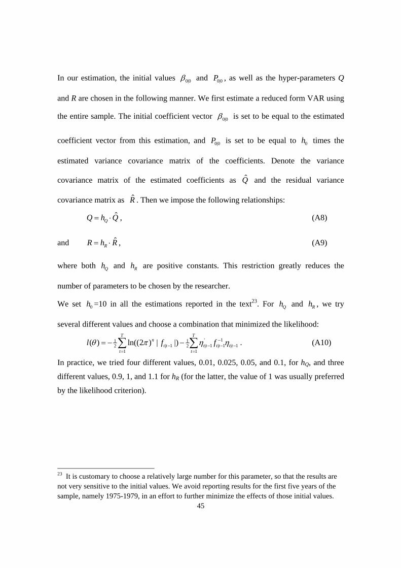
45
In our estimation, the initial values 0|0 and 0|0P , as well as the hyper-parameters Q
and R are chosen in the following manner. We first estimate a reduced form VAR using
the entire sample. The initial coefficient vector 0|0 is set to be equal to the estimated
coefficient vector from this estimation, and 0|0P is set to be equal to 0h times the
estimated variance covariance matrix of the coefficients. Denote the variance
covariance matrix of the estimated coefficients as Q̂ and the residual variance
covariance matrix as R̂ . Then we impose the following relationships:
ˆQQ h Q , (A8)
and ˆRR h R , (A9)
where both Qh and Rh are positive constants. This restriction greatly reduces the
number of parameters to be chosen by the researcher.
We set 0h =10 in all the estimations reported in the text23. For Qh and Rh , we try
several different values and choose a combination that minimized the likelihood:
' 11 1| 1 | 1 | 1 | 12 2
1 1
( ) ln((2 ) | |)T T
nt t t t t t t t
t t
l f f
. (A10)
In practice, we tried four different values, 0.01, 0.025, 0.05, and 0.1, for hQ, and three
different values, 0.9, 1, and 1.1 for hR (for the latter, the value of 1 was usually preferred
by the likelihood criterion).
23 It is customary to choose a relatively large number for this parameter, so that the results are not very sensitive to the initial values. We avoid reporting results for the first five years of the sample, namely 1975-1979, in an effort to further minimize the effects of those initial values.
Top Related