


Languages
Pages
Legal

Investigation of Channel Adaptation and
Interference for Multiantenna OFDM
by
Daniel Vaz Pato Figueiredo, MSc
Dissertation
Presented to the Faculty of Engineering and Science of
Aalborg University
in Partial Fulfillment of the Requirements for the Degree of
Doctor of Philosophy
Aalborg University
Department of Electronic Systems
February 2008

Supervisors
Prof. Ramjee Prasad, Aalborg University, Denmark
Assoc. Prof. Troels Bundgaard Sørensen, Aalborg University, Denmark
Assessment Committee
Prof. Preben Elgaard Mogensen, Aalborg University, Denmark (Chairman)
Prof. Mary Ann Ingram, Georgia Institute of Technology, USA
Assoc. Prof. Antonio Jose Castelo Branco Rodrigues, Technical University of Lisbon,
Portugal
Moderator
Assoc. Prof. Flemming Bjerge Frederiksen, Aalborg University, Denmark
ISBN: 978-87-92328-01-4
Copyright c© 2008 by Daniel Vaz Pato Figueiredo
The copyright of this thesis is held by the author, and no quotation from it or information
derived from it may be published without the acknowledging the source of the information.

Abstract
The new use of internet through social networks, combined with popular bandwidth con-
suming applications, and the need to deliver high data rate connections to highly mobile
users, is the driving force behind the requirements for future wireless networks. In this
context, spectral efficient techniques constitute vital improvements in high data rate ser-
vices. The design of robust systems is an essential factor in coping with the random and
dynamic nature of the multipath in the wireless environment.
This thesis focuses on multiantenna Orthogonal Frequency Division Multiplexing
(OFDM) processing applied with the purpose of increasing the signal strength, of boosting
the data rate, and of increasing the reliability of the wireless link. The author investi-
gates the interaction between different multiantenna processing algorithms and downlink
adaptive transmission, based on link quality information in time-varying channels.
A tradeoff between spatial diversity and multiplexing is offered by the linear dis-
persion framework for space-frequency processing. This thesis evaluates the performance
of the unitary trace orthogonal design, along with linear receivers and channel coding,
and its interaction with link adaptation. Although this coding scheme achieves a superior
performance for low rate modes, the inter-stream interference effect on the probability of
error imposes a poor performance for high order modulations.
In high mobility scenarios, the performance of channel-aware transmission adapta-
tion is highly dependent on the feedback delay. This thesis develops an analytical frame-
work designed to investigate the performance of rate adaptation in a time-varying channel
for selected Multiple Input Multiple Output (MIMO) schemes: spatial diversity, multiplex-
iii

iv
ing, and antenna selection. The probability of bit error is evaluated in a Rayleigh scenario
for a rate adaptive system operating on outdated channel information, and closed-form
expressions for the average probability of error are derived for each MIMO scheme. As a
result, we propose analytical thresholds for rate adaptation, based on outdated channel
information. In continuation, this thesis, supported by the study of the robustness of the
feedback channel, proposes a mechanism to select the modulation and MIMO scheme in
a multimode transmission system.
The effect of cochannel signals in a cellular scenario is studied in analytical and sim-
ulation contexts to assess the performance of spatial diversity and OFDM transmissions.
On the basis of an analytical framework, we detect a relation between the number of inter-
fering sources on the probability of error of a high-order spatial diversity link. In cellular
systems, a suboptimal interference cancelation, for the downlink inter-cell interference, is
shown to attain significant performance for a single transmit antenna, but a limited effect
for spatial transmit diversity, due to its sensitivity to channel estimation error.
Besides the concrete solution proposals, the thesis leads to a better understanding
of practical aspects from integration of MIMO in wireless scenarios.
Aalborg University
Dansk Resume
Den nye brug af Internettet baseret pa sociale netværk i kombination med populære
bredbandsbaserede applikationer, og behovet for at levere høje dataoverførselshastigheder
til mobile brugere, er de drivende kræfter bag kravene til fremtidens tradløse netværk. Set
i denne sammenhæng udgør spektraleffektive teknologier en væsentlig del af de forventede
forbedringer til dataintensive services. Designet af robuste systemer er en essentiel faktor
i handteringen af den tilfældige og dynamiske karakter af flervejsudbredelse i tradløse
scenarier.
Denne afhandling fokuserer pa multiantenne processering i Orthogonal Frequen-
cy Division Multiplexing (OFDM) anvendt med henblik pa at øge signalstyrken, forøge
dataoverførselshastigheden og øge palideligheden i den tradløse forbindelse. Forfatteren
undersøger interaktionen mellem forskellige multiantenne processeringsalgoritmer og adap-
tive transmission i downlink baseret pa link kvalitetsinformation i tidsvarierende kanaler.
En afvejning mellem diversity og multipleksing er mulig ved hjælp af en model
for lineær spredning i rum og frekvens. Afhandlingen evaluerer ydeevnen af unitary tra-
ce orthogonal design med lineære modtagere og kanalkodning, samt interaktionen med
linkadaptering. Selvom den lineære spredningskodning opnar overlegen ydeevne ved lav
modulationsorden, betyder indvirkningen pa fejlsandsynligheden fra interferens mellem
de transmitterede datastrømme en darligere ydelse ved høj modulationsorden.
I scenarier med høj mobilitet, er ydeevnen af den kanaladaptive transmission særde-
les afhængig af forsinkelsen pa kanalinformationen. Denne afhandling udvikler en analy-
tisk model for ydeevnen af kanaladaptiv transmission i en tidsvariende kanal for udvalgte
v

vi
Multiple Input Multiple Output (MIMO) systemer baseret pa diversity, multipleksing og
antenneselektion. Sandsynligheden for bitfejl er evalueret for et scenarie med Rayleigh-
kanal og kanaltilpasning baseret pa uddateret kanalinformation. I denne sammenhæng er
der udledt lukkede udtryk for middel fejlsandsynligheden for hvert MIMO system. Som
resultat heraf anbefales analytisk udledte tærskelværdier for kanaltilpasningen under hen-
syntagen til den uddaterede kanalinformation. I forlængelse heraf, og baseret pa studiet
af feedback, anbefales en mekanisme til at vælge modulation og MIMO system i et mulit-
modalt transmissionssystem.
Effekten af co-channel signaler i et cellulært scenarie er undersøgt analytisk og ved
simulering for at male ydeevnen af diversity i OFDM transmission. Pa basis af den analy-
tiske udledning er der bestemt en sammenhæng mellem antallet af interfererende signaler
og fejlsandsynligheden i et MIMO diversity system. I et cellulært system med downlink
inter-celle interferens er det vist at en suboptimal interferensudligner opnar en betydelig
ydeevne i tilfældet med en enkelt senderantenne, mens flere senderantenner har en be-
grænset effekt pa grund af følsomheden overfor kanalestimeringsfejl i dette sidste tilfælde.
Ud over de konkrete løsningsforslag bidrager afhandlingen til en øget forstaelse af
de praktisk relaterede aspekter vedrørende integrationen af MIMO i tradløse scenarier.
Aalborg University

Dedicated to my beloved family and friends.


Preface and Acknowledgments
The work in this dissertation is the result of research carried out at the Department of
Electronic Systems at Aalborg University, Denmark. The research has been co-financed
by Samsung Electronics, the Department of Electronic Systems, and the European Union.
The contributions of the thesis are presented in Chapters 2–5. The reader unfamiliar with
the technical concepts addressed in the contributions may profit from the introductory
background in Appendices A–E for a better understanding of the technical details of the
description of contributions.
In the first place, I am grateful to Ramjee Prasad for his support and for having
believed in my success until the end. Special thanks to Troels Sørensen that supervised
me during the second part of the Ph.D. for the significant contribution in making this
thesis a reality. I would like to thank to the guidance given during earlier stages of my
Ph.D. studies from Frank Fitzek, Elisabeth de Carvalho, and Zihuai Lin.
I would like to leave a word of gratitude to my colleagues and friends of the Wireless
Networking Group (WING) and fellow Ph.D. students in the JADE project. Muhmmad
Imadur Rahman has been an amazing colleague that always supported me, and with
whom I have learned a lot. Together with Nicola Marchetti and Suvra Das we have had
many fruitful discussions. I would also like to express my gratitude to my colleagues at
the Radio Access Technology (RATE) section that made a very friendly and productive
working environment, without forgetting the very competitive table tennis matches after
lunch.
I am thankful to the friends I have made during my stay at Aalborg, they are the
support and kindness I needed for living far away from home. I will keep in my heart the
new family we have imagined in the early days at Aalborg. The biggest thanks to my
ix

x PREFACE AND ACKNOWLEDGMENTS
girlfriend Dalia Tiesyte for the support, the patience, the travels, and the proof-reading
of this thesis. In my mind are and will always be my home friends back in Lisbon.
Finally, I would like to thank my family in Portugal, and, especially, my parents,
brother, and sister for their full support, patience, entertaining phone calls, and writing
advice.
Daniel Vaz Pato Figueiredo
Aalborg University
February 2008
Aalborg University

Contents
Preface and Acknowledgments ix
List of Figures xvii
List of Tables xxi
List of Symbols xxiii
List of Acronyms xxv
Chapter 1 Introduction 1
1.1 Motivation . . . . . . . . . . . . . . . . . . . . . . . . . . . . . . . . . . . . 1
1.2 State-of-the-Art . . . . . . . . . . . . . . . . . . . . . . . . . . . . . . . . . . 3
1.2.1 OFDM . . . . . . . . . . . . . . . . . . . . . . . . . . . . . . . . . . 3
1.2.2 MIMO . . . . . . . . . . . . . . . . . . . . . . . . . . . . . . . . . . . 4
1.2.3 Adaptation and Scheduling . . . . . . . . . . . . . . . . . . . . . . . 6
1.3 Challenges and Goals . . . . . . . . . . . . . . . . . . . . . . . . . . . . . . . 8
1.4 Outline and Contributions . . . . . . . . . . . . . . . . . . . . . . . . . . . . 9
Chapter 2 Beamforming and Space-Time Processing in OFDM 13
2.1 Space-Time Linear Model . . . . . . . . . . . . . . . . . . . . . . . . . . . . 14
2.2 Beamforming and Spatial Diversity in OFDM Systems . . . . . . . . . . . . 15
2.2.1 Beamforming . . . . . . . . . . . . . . . . . . . . . . . . . . . . . . . 16
2.2.2 Spatial Diversity . . . . . . . . . . . . . . . . . . . . . . . . . . . . . 17
xi
xii CONTENTS
2.2.3 Space-Frequency or Space-Time Processing and Scheduling . . . . . 18
2.2.4 Results . . . . . . . . . . . . . . . . . . . . . . . . . . . . . . . . . . 20
2.2.5 Summary . . . . . . . . . . . . . . . . . . . . . . . . . . . . . . . . . 25
2.3 MIMO and Rate Adaptation in OFDM . . . . . . . . . . . . . . . . . . . . 25
2.3.1 System Model . . . . . . . . . . . . . . . . . . . . . . . . . . . . . . . 26
2.3.2 Linear Dispersion Codes Model . . . . . . . . . . . . . . . . . . . . . 27
2.3.3 Performance of LDC . . . . . . . . . . . . . . . . . . . . . . . . . . . 30
2.3.4 Summary . . . . . . . . . . . . . . . . . . . . . . . . . . . . . . . . . 34
2.4 Conclusions . . . . . . . . . . . . . . . . . . . . . . . . . . . . . . . . . . . . 35
Chapter 3 Feedback Delay in Rate Adaptive MIMO 37
3.1 Link and System Implications from Outdated Feedback . . . . . . . . . . . 38
3.1.1 Preliminary Evaluation of Outdated Channel . . . . . . . . . . . . . 40
3.1.2 Summary . . . . . . . . . . . . . . . . . . . . . . . . . . . . . . . . . 44
3.2 Analytical Performance of Rate Adaptation . . . . . . . . . . . . . . . . . . 44
3.2.1 Evaluation of Analytical Performance . . . . . . . . . . . . . . . . . 46
3.2.2 Results and Discussion . . . . . . . . . . . . . . . . . . . . . . . . . . 48
3.2.3 Summary . . . . . . . . . . . . . . . . . . . . . . . . . . . . . . . . . 49
3.3 Channel Power Prediction . . . . . . . . . . . . . . . . . . . . . . . . . . . . 50
3.3.1 Power Prediction . . . . . . . . . . . . . . . . . . . . . . . . . . . . . 51
3.3.2 MIMO Diversity . . . . . . . . . . . . . . . . . . . . . . . . . . . . . 51
3.3.3 MIMO Multiplexing . . . . . . . . . . . . . . . . . . . . . . . . . . . 52
3.3.4 Antenna Selection . . . . . . . . . . . . . . . . . . . . . . . . . . . . 53
3.3.5 Evaluation of Analytical Performance . . . . . . . . . . . . . . . . . 53
3.3.6 Summary . . . . . . . . . . . . . . . . . . . . . . . . . . . . . . . . . 56
3.4 Practical System Aspects . . . . . . . . . . . . . . . . . . . . . . . . . . . . 58
3.4.1 SISO thresholds for MIMO . . . . . . . . . . . . . . . . . . . . . . . 58
3.4.2 Generic versus Updated Thresholds . . . . . . . . . . . . . . . . . . 59
3.4.3 Summary . . . . . . . . . . . . . . . . . . . . . . . . . . . . . . . . . 60
Aalborg University

CONTENTS xiii
3.5 Conclusions . . . . . . . . . . . . . . . . . . . . . . . . . . . . . . . . . . . . 61
Chapter 4 Adaptive MIMO-OFDMA Mechanisms 63
4.1 System Description . . . . . . . . . . . . . . . . . . . . . . . . . . . . . . . . 64
4.1.1 Performance of MIMO Modes with Outdated Feedback . . . . . . . 66
4.1.2 Histogram of Modulation Levels . . . . . . . . . . . . . . . . . . . . 69
4.2 Transmit Strategy . . . . . . . . . . . . . . . . . . . . . . . . . . . . . . . . 71
4.2.1 MIMO Look-up Tables . . . . . . . . . . . . . . . . . . . . . . . . . . 75
4.2.2 Summary . . . . . . . . . . . . . . . . . . . . . . . . . . . . . . . . . 80
4.3 Feedback Design Issues . . . . . . . . . . . . . . . . . . . . . . . . . . . . . . 80
4.3.1 Reporting SNR of a Frame . . . . . . . . . . . . . . . . . . . . . . . 80
4.3.2 Length of Delay between Frames . . . . . . . . . . . . . . . . . . . . 81
4.3.3 Summary . . . . . . . . . . . . . . . . . . . . . . . . . . . . . . . . . 84
4.4 Conclusions . . . . . . . . . . . . . . . . . . . . . . . . . . . . . . . . . . . . 84
Chapter 5 Cochannel Interference and Asynchronous OFDM 85
5.1 Effect of Cochannel Interference on Spatial Diversity . . . . . . . . . . . . . 86
5.1.1 System Model . . . . . . . . . . . . . . . . . . . . . . . . . . . . . . . 87
5.1.2 Channel Statistics for Diversity and Interference . . . . . . . . . . . 88
5.1.3 Average Probability of Bit Error . . . . . . . . . . . . . . . . . . . . 90
5.1.4 Results and Discussion . . . . . . . . . . . . . . . . . . . . . . . . . . 91
5.1.5 Summary . . . . . . . . . . . . . . . . . . . . . . . . . . . . . . . . . 95
5.2 Asynchronous Cochannel Signals in Cellular OFDM Systems . . . . . . . . 95
5.2.1 System Model . . . . . . . . . . . . . . . . . . . . . . . . . . . . . . . 96
5.2.2 Effect of Cochannel Signals in Broadcast . . . . . . . . . . . . . . . . 99
5.2.3 Effect of Cochannel Signals in Unicast . . . . . . . . . . . . . . . . . 102
5.2.4 Known Interference with MMSE Detection . . . . . . . . . . . . . . 104
5.2.5 Summary . . . . . . . . . . . . . . . . . . . . . . . . . . . . . . . . . 107
5.3 Conclusions . . . . . . . . . . . . . . . . . . . . . . . . . . . . . . . . . . . . 109
Daniel Vaz Pato Figueiredo

xiv CONTENTS
Chapter 6 Conclusions and Future Work 111
6.1 Future Work . . . . . . . . . . . . . . . . . . . . . . . . . . . . . . . . . . . 113
Appendix A Wireless Channel 115
A.1 Propagation Path Loss and Shadowing . . . . . . . . . . . . . . . . . . . . . 115
A.2 Mobility and Multipath . . . . . . . . . . . . . . . . . . . . . . . . . . . . . 116
A.2.1 Doppler Effect . . . . . . . . . . . . . . . . . . . . . . . . . . . . . . 118
A.2.2 Coherence Bandwidth and Coherence Time . . . . . . . . . . . . . . 119
A.2.3 Angular Spread . . . . . . . . . . . . . . . . . . . . . . . . . . . . . . 120
Appendix B OFDM 121
B.1 OFDM Overview . . . . . . . . . . . . . . . . . . . . . . . . . . . . . . . . . 121
B.1.1 OFDM Statistical Model . . . . . . . . . . . . . . . . . . . . . . . . 124
Appendix C Antenna Arrays 127
C.1 Uniform Linear Arrays . . . . . . . . . . . . . . . . . . . . . . . . . . . . . . 127
C.2 Beamforming . . . . . . . . . . . . . . . . . . . . . . . . . . . . . . . . . . . 128
Appendix D Antenna Diversity 131
D.1 Receive Diversity . . . . . . . . . . . . . . . . . . . . . . . . . . . . . . . . . 132
D.2 Transmit Diversity . . . . . . . . . . . . . . . . . . . . . . . . . . . . . . . . 133
D.2.1 Space-Time Coding . . . . . . . . . . . . . . . . . . . . . . . . . . . 133
D.2.2 Space-Frequency Coding . . . . . . . . . . . . . . . . . . . . . . . . . 134
D.3 SNR Statistics . . . . . . . . . . . . . . . . . . . . . . . . . . . . . . . . . . 134
D.3.1 Spatial Diversity . . . . . . . . . . . . . . . . . . . . . . . . . . . . . 135
D.3.2 Spatial Multiplexing . . . . . . . . . . . . . . . . . . . . . . . . . . . 137
D.3.3 Antenna Selection . . . . . . . . . . . . . . . . . . . . . . . . . . . . 137
Appendix E Adaptation and Scheduling 139
E.1 Adaptive Modulation . . . . . . . . . . . . . . . . . . . . . . . . . . . . . . . 139
E.2 Multiuser Scheduling . . . . . . . . . . . . . . . . . . . . . . . . . . . . . . . 141
Aalborg University

CONTENTS xv
Appendix F Statistics of SNR and Analytical BER Using Prediction 145
F.1 Unbiased Power Predictor . . . . . . . . . . . . . . . . . . . . . . . . . . . . 145
F.2 Distribution of Predicted SNR for MIMO . . . . . . . . . . . . . . . . . . . 147
F.2.1 SISO . . . . . . . . . . . . . . . . . . . . . . . . . . . . . . . . . . . . 148
F.2.2 Spatial Multiplexing . . . . . . . . . . . . . . . . . . . . . . . . . . . 149
F.2.3 MIMO Diversity . . . . . . . . . . . . . . . . . . . . . . . . . . . . . 151
F.2.4 Antenna Selection . . . . . . . . . . . . . . . . . . . . . . . . . . . . 155
F.3 M-QAM Performance . . . . . . . . . . . . . . . . . . . . . . . . . . . . . . 156
F.3.1 SISO . . . . . . . . . . . . . . . . . . . . . . . . . . . . . . . . . . . . 156
F.3.2 Spatial Multiplexing . . . . . . . . . . . . . . . . . . . . . . . . . . . 157
F.3.3 MIMO Diversity . . . . . . . . . . . . . . . . . . . . . . . . . . . . . 158
F.3.4 Antenna Selection . . . . . . . . . . . . . . . . . . . . . . . . . . . . 159
Appendix G Link Simulator EUTRA 161
Appendix H Dissemination of Results 165
Bibliography 169
Vita 183
Daniel Vaz Pato Figueiredo


List of Figures
1.1 Evolution of global standards . . . . . . . . . . . . . . . . . . . . . . . . . . 2
2.1 Time domain beamforming in OFDM . . . . . . . . . . . . . . . . . . . . . 19
2.2 Frequency domain beamforming in OFDM . . . . . . . . . . . . . . . . . . . 20
2.3 STBC and SFBC in OFDM . . . . . . . . . . . . . . . . . . . . . . . . . . . 20
2.4 BER performance of transmit diversity for different angular spread . . . . . 23
2.5 BER performance of beamforming and STBC for indoor channel . . . . . . 24
2.6 BER performance of beamforming and SFBC for outdoor channel . . . . . 24
2.7 System model with MIMO and AMC . . . . . . . . . . . . . . . . . . . . . . 26
2.8 Uncoded BER in MIMO 2 × 2 configuration . . . . . . . . . . . . . . . . . . 31
2.9 Spectral efficiency in MIMO 2 × 2 with fixed modulation . . . . . . . . . . . 32
2.10 Spectral efficiency in MIMO 2 × 2 with link adaptation . . . . . . . . . . . 33
2.11 Probability of bit error of an uncoded system in MIMO 2 × 4 with fixed
modulation . . . . . . . . . . . . . . . . . . . . . . . . . . . . . . . . . . . . 33
2.12 Spectral efficiency in MIMO 2 × 4 with link adaptation . . . . . . . . . . . 34
3.1 System model of MIMO and adaptive modulation . . . . . . . . . . . . . . 39
3.2 Single-user scenario . . . . . . . . . . . . . . . . . . . . . . . . . . . . . . . . 43
3.3 Ten users scenario with scheduler max-SNR . . . . . . . . . . . . . . . . . . 43
3.4 Average BER of a discrete M-QAM adaptive system. Analytical versus
simulation results . . . . . . . . . . . . . . . . . . . . . . . . . . . . . . . . . 49
3.5 Average BER of a discrete M-QAM adaptive system with delay . . . . . . . 50
xvii

xviii LIST OF FIGURES
3.6 BER for different M-QAM levels . . . . . . . . . . . . . . . . . . . . . . . . 54
3.7 Adaptive M-QAM (M=0,4,16,64,256) over Rayleigh fading channel . . . . . 55
3.8 BER curves of SISO for different values of relative error variance . . . . . . 55
3.9 BER curves for different MIMO techniques . . . . . . . . . . . . . . . . . . 56
3.10 Average BER for different MIMO techniques . . . . . . . . . . . . . . . . . 57
3.11 Average effective throughput for different MIMO techniques . . . . . . . . . 57
3.12 Average effective throughput for different MIMO techniques. Updated ver-
sus SISO thresholds . . . . . . . . . . . . . . . . . . . . . . . . . . . . . . . 59
3.13 Average BER for MIMO techniques. Updated versus generic thresholds . . 60
4.1 System model of MIMO and adaptive modulation . . . . . . . . . . . . . . 65
4.2 LOC and DIV subchannels within an OFDM frame . . . . . . . . . . . . . . 66
4.3 Spectral efficiency of system with no delay . . . . . . . . . . . . . . . . . . . 67
4.4 Spectral efficiency of system with fdτ = 0.06 and generic thresholds . . . . 68
4.5 Spectral efficiency of system with fdτ = 0.06 and updated thresholds . . . . 69
4.6 Modulation histogram of SISO with generic thresholds . . . . . . . . . . . . 70
4.7 Modulation histogram of SISO with updated thresholds and normalized
delay fdτ = 0.1 . . . . . . . . . . . . . . . . . . . . . . . . . . . . . . . . . . 71
4.8 Flowchart of MIMO switching mechanism . . . . . . . . . . . . . . . . . . . 74
4.9 Flowchart for downlink MISO 2 × 1 configuration . . . . . . . . . . . . . . . 74
4.10 Flowchart for downlink MIMO 2 × 2 configuration . . . . . . . . . . . . . . 75
4.11 MISO 2 × 1 look-up table . . . . . . . . . . . . . . . . . . . . . . . . . . . . 76
4.12 Spectral efficiency of MISO 2 × 1 look-up table with no delay . . . . . . . . 77
4.13 Spectral efficiency of MISO 2 × 1 look-up table with fdτ = 0.10 . . . . . . . 77
4.14 MIMO 2 × 2 look-up table . . . . . . . . . . . . . . . . . . . . . . . . . . . . 78
4.15 Spectral efficiency of MIMO 2 × 2 look-up table with no delay . . . . . . . . 79
4.16 Spectral efficiency of MIMO 2 × 2 look-up table with fdτ = 0.09 . . . . . . 79
4.17 Reporting the SNR of a frame . . . . . . . . . . . . . . . . . . . . . . . . . . 81
4.18 Spectral efficiency for different reported SNR with fdτ = 0.1 . . . . . . . . . 82
Aalborg University

LIST OF FIGURES xix
4.19 Different durations for designing AMC thresholds . . . . . . . . . . . . . . . 82
4.20 Spectral efficiency of different AMC thresholds with fdτ = 0.1 . . . . . . . . 83
5.1 System model of MIMO desired link with multiple single antenna cochannel
interferers . . . . . . . . . . . . . . . . . . . . . . . . . . . . . . . . . . . . . 87
5.2 Average BER versus the number of interferers with high power . . . . . . . 92
5.3 Average BER versus the number of interferers with low power . . . . . . . . 93
5.4 Average bit error rate versus the number of interferers when the SINR
remains constant . . . . . . . . . . . . . . . . . . . . . . . . . . . . . . . . . 94
5.5 Cellular scenario for a cell radius of 1000 m . . . . . . . . . . . . . . . . . . 98
5.6 Average power of the channel paths of a terminal in position C of the cellular
layout with cell radius 1000 m . . . . . . . . . . . . . . . . . . . . . . . . . . 99
5.7 Effect of single interferer delays in broadcast . . . . . . . . . . . . . . . . . 100
5.8 Spectral efficiency of downlink cellular broadcast system for different cell
radius . . . . . . . . . . . . . . . . . . . . . . . . . . . . . . . . . . . . . . . 101
5.9 Spectral efficiency of downlink cellular broadcast system for different cell
radius . . . . . . . . . . . . . . . . . . . . . . . . . . . . . . . . . . . . . . . 102
5.10 Effect of single interferer delays in unicast . . . . . . . . . . . . . . . . . . . 103
5.11 Spectral efficiency for different positions in the cell. Unicast signal with
QPSK and MRC receiver . . . . . . . . . . . . . . . . . . . . . . . . . . . . 104
5.12 Spectral efficiency for different positions in the cell. Unicast signal and
16-QAM . . . . . . . . . . . . . . . . . . . . . . . . . . . . . . . . . . . . . . 105
5.13 Spectral efficiency for different positions in the cell. Unicast signal with
QPSK and MMSE receiver . . . . . . . . . . . . . . . . . . . . . . . . . . . 105
5.14 Spectral efficiency for receivers MRC, MMSE, and Window-MMSE for
SIMO configuration. Unicast signal and 16-QAM . . . . . . . . . . . . . . . 107
5.15 Spectral efficiency for receivers MRC, MMSE, and Window-MMSE for
MIMO diversity. Unicast signal with 16-QAM . . . . . . . . . . . . . . . . . 108
A.1 Rice distribution vector . . . . . . . . . . . . . . . . . . . . . . . . . . . . . 117
Daniel Vaz Pato Figueiredo

xx LIST OF FIGURES
A.2 Angular spread at the BS and the MS . . . . . . . . . . . . . . . . . . . . . 120
B.1 OFDM transceiver model . . . . . . . . . . . . . . . . . . . . . . . . . . . . 122
B.2 Spectrum of an OFDM subcarrier (left) and a combined OFDM signal with
three subcarriers overlapped (right) . . . . . . . . . . . . . . . . . . . . . . . 123
B.3 OFDM symbol in time domain . . . . . . . . . . . . . . . . . . . . . . . . . 123
B.4 Model of an OFDM transmitter (above) and receiver (under) . . . . . . . . 124
C.1 Uniformly spaced linear array . . . . . . . . . . . . . . . . . . . . . . . . . . 128
E.1 BER of M-ary QAM over flat fading channel and thresholds for instanta-
neous BER constraint . . . . . . . . . . . . . . . . . . . . . . . . . . . . . . 140
G.1 Block diagram of link-level simulator . . . . . . . . . . . . . . . . . . . . . . 162
Aalborg University
List of Tables
2.1 Half rate space-time encoding scheme . . . . . . . . . . . . . . . . . . . . . 18
4.1 Available MIMO modes . . . . . . . . . . . . . . . . . . . . . . . . . . . . . 72
4.2 Selection criterion for the transmit strategy in MISO 2 × 1 . . . . . . . . . . 73
4.3 Selection criterion for the transmit strategy in MIMO 2 × 2 . . . . . . . . . 73
A.1 Channel RMS delay spread . . . . . . . . . . . . . . . . . . . . . . . . . . . 118
A.2 Channel coherence time at 5 GHz . . . . . . . . . . . . . . . . . . . . . . . . 120
xxi


List of Symbols
fc Carrier frequencyB Bandwidthλ WavelengthBc Coherence bandwidthTc Coherence timefd Doppler frequency
d Data vectors Transmitted signal vectorh Channel coefficients vectorH Channel coefficients matrixy Received signal vectorw Noise vector
Es Transmitted signal powerN0 Noise powerγ Signal to noise ratio at the receiverγb Signal to noise ratio per bit at the receiverρa Signal to noise ratio per receiver antenna
Nt Number of transmit antennasNr Number of receive antennasq Transmit antenna indexp Receive antenna indexNa Number of receive/transmit antennas for SM
T Number of channel uses in the ST codeNs Number of symbols in the ST codeY Received signal block matrixS Transmitted signal block matrixW Noise block matrix
xxiii

xxiv LIST OF SYMBOLS
F Discrete Fourier TransformN Number of OFDM subcarriersk Subcarrier indexNd Number of data subcarriersTs Total OFDM symbol durationTf Frame duration
M Modulation orderR Number of constellationsb Bit per modulation symbolPb or BER Bit error probabilityPs Symbol error probabilityη Throughput
ρ Time correlationτ Time delayψ Delay/prediction thresholds for MIMO selection
n Time domain indexγ Predicted SNR at the receiverυhǫh Relative variance of the prediction error
h Predicted channel coefficientǫh Channel prediction errorp Channel powerp Predicted channel powerǫp Predicted channel power error
L Number of interferersEi Interference signal powerg Interference channel vector responseρI Interference to noise ratio at the receiver
Aalborg University
List of Acronyms
2G Second Generation
3G Third Generation
3GPP The Third Generation Partnership Project
4G Fourth Generation
AMC Adaptive Modulation and Coding
AS Antenna Selection
AWGN Additive White Gaussian Noise
BER Bit Error Rate
BLER Block Error Rate
BPSK Binary Phase Shift Keying
BS Base Station
CCI Cochannel Interference
CDF Cumulative Distribution Function
CIR Channel Impulse Response
CP Cyclic Prefix
CRC Cyclic Redundancy Check
CSI Channel State Information
DAB Digital Audio Broadcasting
DIV Diversity
xxv

xxvi LIST OF ACRONYMS
DFT Discrete Fourier Transform
DoA Direction of Arrival
DoD Direction of Departure
DSL Digital Subscriber Line
DVB Digital Video Broadcasting
EESM Exponential Effective SNR Mapping
E-UTRA Evolved UMTS Terrestrial Radio Access
FDD Frequency Division Duplex
FDM Frequency Division Multiplexing
FFT Fast Fourier Transform
HARQ Hybrid Automatic Repeat Request
HSPA High-Speed Packet Access
ICI Inter-Carrier Interference
IDFT Inverse Discrete Fourier Transform
IEEE Institute of Electrical and Electronics Engineers
IFFT Inverse Fast Fourier Transform
INR Interference to Noise Ratio
ISD Inter-Site Distance
ISI Inter-Symbol Interference
ISR Interference to Signal Ratio
LDC Linear Dispersion Codes
LOC Localized
LOS Line of Sight
LS Least-Square
LTE Long Term Evolution
MCS Modulation Code Schemes
Aalborg University

LIST OF ACRONYMS xxvii
MIMO Multiple Input Multiple Output
MISO Multiple Input Single Output
MMSE Minimum Mean Square Error
MRC Maximal Ratio Combining
MS Mobile Station
MSE Mean Square Error
MUD Multiuser Diversity
NLOS Non Line of Sight
OFDM Orthogonal Frequency Division Multiplexing
OFDMA Orthogonal Frequency Division Multiple Access
PAPR Peak to Average Power Ratio
PARC Per Antenna Rate Control
PDF Probability Density Function
PDP Power Delay Profile
PSK Phase Shift Keying
QAM Quadrature Amplitude Modulation
QoS Quality of Service
QPSK Quadrature Phase Shift Keying
RMS Root Mean Square
SFBC Space-Frequency Block Code
SFC Space-Frequency Coding
SIMO Single Input Multiple Output
SINR Signal to Interference and Noise Ratio
SIR Signal to Interference Ratio
SISO Single Input Single Output
SM Spatial Multiplexing
Daniel Vaz Pato Figueiredo

xxviii LIST OF ACRONYMS
SNR Signal to Noise Ratio
SVD Singular Value Decomposition
STBC Space-Time Block Code
STC Space-Time Coding
TDD Time Division Duplex
TDMA Time Division Multiple Access
UTRA UMTS Terrestrial Radio Access
UTOD Unitary Trace Orthogonal Design
WCDMA Wideband Code Division Multiple Access
WAN Wide Area Network
WiMAX Worldwide Interoperability for Microwave Access
WLAN Wireless Local Area Network
ZF Zero Forcing
Aalborg University

Chapter 1
Introduction
Over the last two decades, wireless communications have been enthusiastically accepted by
the world’s population a large, to become an essential tool in our day-to-day lives. This
is largely due to the Second Generation (2G) wireless systems. Although 2G networks
focused on delivering speech services, the explosion of internet connections in the home,
along with increasing availability of broadband connections has created a considerable
demand for wireless data services. Moreover, bandwidth intensive or high-speed appli-
cations, such as media streaming offered by YouTube and other media sharing sites, are
expected to drive huge demands on wireless networks’ resources, as they become available
in mobile devices. Once the growth in social networks, such as Facebook and MySpace, is
extended to wireless networks, the multimedia sharing experience enters the next level of
anytime and anywhere access to one’s community.
1.1 Motivation
Designed to enable the access to broadband connection through a cellular phone, the
Third Generation (3G) was introduced by The Third Generation Partnership Project
(3GPP). This project promised peak data rates to the order of 10 Mbit/s along with
Wideband Code Division Multiple Access (WCDMA) and High-Speed Packet Access
(HSPA) [HT04, HT06]. In parallel, other development groups within the 802 family of
1

2 Chapter 1. Introduction
LTEHSPA
802.16eM-WiMAX
WCDMA
Peak data rate
Mob
ility
low(pedestrian)
medium(vehicular
city)
high(vehicular highway)
1 Mbit/s 50 Mbit/s 100 Mbit/s 1 Gbit/s
2000 2005 2010
802.16dF-WiMAX
802.11b/g
802.11n
4G3G2Gseamless
connectivity across
heterogeneous networks
��������You Tube
Figure 1.1: Evolution of global standards
the Institute of Electrical and Electronics Engineers (IEEE) standards promote nomadic
broadband wireless data access that have led to the the popular Wireless Local Area
Networks (WLANs), 802.11b/g, and the fixed Worldwide Interoperability for Microwave
Access (WiMAX), known as 802.16d-2004 [IEE04].
Along the path to Fourth Generation (4G) systems, even higher spectral efficiency
is sought to achieve a data rate within the order of 100 Mbit/s in mobile outdoor sce-
narios, and 1 Gbit/s in nomadic scenarios. The definition of the 4G systems has not yet
been agreed upon and still awaits standardization and the release of spectrum, whereas
evolutions of 3G systems are expected to be competitive for several years to come. The
mobile WiMAX 802.16e-2005 [IEE06] and the Long Term Evolution (LTE) [3GP06b] of
3GPP are competing as leaders in radio access technology in the direction of 4G systems.
One important requirement for the 4G is the seamless connectivity and smooth handoff
across heterogeneous networks. Figure 1.1 represents the evolution of standards in terms
of data rate and user mobility.
The new requirements for high-speed data are the driving force behind research into
Aalborg University
1.2 State-of-the-Art 3
wireless networks. Thus, several techniques that enhance the spectral efficiency of systems
and allow for an increased throughput with the same spectrum have received considerable
attention from the research community. A fundamental feature of wireless fading channels
is the dynamic random variation of the channel’s strengths. In fact, multipath and mobile
environments introduce fading and uncertainty in the channel, which complicates any
efforts to deliver high-speed data connections. The effect of simply increasing the transmit
power or of using an additional bandwidth may not be the solution to achieve a robust
broadband system [Kim02]. Therefore, advanced physical layer techniques are required
to reduce the effect of fading in both the transmitter and receiver, without excessively
increasing the system’s complexity and cost.
In recent years, several spectral efficient techniques have received considerable inter-
est and support from both the research community and industry. This thesis focuses on
three groups of physical layer techniques: multicarrier transmission, multiantenna process-
ing, and channel-aware schemes. The aim of this thesis is to provide a better understanding
of multiantenna processing integration in the next generation wireless systems. In fact,
multiantenna processing is of particular interest, and several flavors of the technique are
already being supported by the new wireless systems. However, several practical problems
must be addressed regarding the up-coming generations of wireless networks.
1.2 State-of-the-Art
1.2.1 OFDM
OFDM is an effective multicarrier technique that has the ability to cope with the severe
channel characteristics without requiring high complexity equalization receivers [NP00].
OFDM, custom-designed for broadband channels, converts the wideband frequency se-
lective channel into multiple narrowband flat channels. One of the main advantages of
multicarrier systems is that it permits transmission over frequency-selective channels at
a low receiver implementation cost. OFDM is therefore commonly accepted as being the
most effective transmission technology for the downlink of future high data rate broad-
Daniel Vaz Pato Figueiredo

4 Chapter 1. Introduction
band systems [HP03]. However, some drawbacks affect the performance of OFDM in
cellular scenarios. A widely known problem of multicarrier transmission is its vulnera-
bility to synchronization errors. The Doppler shift, caused by high mobility, introduces
Inter-Carrier Interference (ICI), while long multipath delay profiles create Inter-Symbol
Interference (ISI) [HT01].
1.2.2 MIMO
A MIMO system is defined as a system with multiple antennas at the receiver and trans-
mitter ends. Traditionally, multiple antennas were employed to shape the radiation dia-
gram of the antenna pattern, using a technique known as beamforming [App76]. However,
multiple antennas at the transmitter and receiver may be used to exploit array, diversity,
and/or multiplexing gains. In recent years, techniques that transmit over spatially uncor-
related antennas have received broad attention from the research community due to their
potential to increase the reliability or the data rate of the wireless link.
Spatial diversity and multiplexing are effective techniques to increase robustness and
the data rate in wireless systems requiring low complexity. MIMO transmission schemes
that assume channel knowledge at the receiver, but not at the transmitter, mainly deliver
spatial diversity or multiplexing gains.
Spatial diversity techniques have been proposed to overcome wireless channel im-
pairments by providing a more reliable transmission link. Spatial diversity can be ex-
ploited at the receiver by employing Maximal Ratio Combining (MRC) which uses the
knowledge of the channel’s coefficients to achieve both array and diversity gains. The
technique designed to encode multiantenna transmissions is referred to as Space-Time
Coding (STC) [PNG03, GSS+03]. STC schemes map the source symbols to the trans-
mit antennas. These schemes were popularized with the discovery of Space-Time Block
Code (STBC). STBC, introduced by [Ala98, TJC99], is an open-loop transmit diver-
sity scheme whose diversity gain is achieved without the knowledge of the channel at the
transmitter by employing linear receivers.
Aalborg University

1.2 State-of-the-Art 5
As opposed to diversity techniques, the MIMO channel can be used for Spatial
Multiplexing (SM), in order to dramatically increase the system throughput [Tel95, Fos96].
The MIMO configuration is applied so as to create parallel streams of data by using SM.
This technique boosts the data rate by using the multiple spatial links to transmit more
symbols, albeit at the cost of diversity gain.
More recently, the authors in [HH02] have introduced the Linear Dispersion Codes
(LDC) framework that generalizes the design of encoding schemes in the space-time or
space-frequency domains. This approach provides a linear model of the transmission
where spatial diversity and spatial multiplexing may be regarded as particular cases of
encoding. Space-time codes that present full diversity and full rate have been proposed.
These include rotation of constellations [SP04], non-linear processing [HG03, FB06], or
complex-field precoding [MG03].
MIMO-OFDM OFDM itself does not offer any built-in diversity, and in many cases
it is desirable to introduce robustness in the wireless link. To obtain a more robust sys-
tem, multiantenna techniques can be used to deliver array, diversity, and/or multiplexing
gains. Since, in OFDM, each subcarrier experiences a flat fading input-output relation,
MIMO-OFDM systems can use narrowband multiantenna schemes at each subcarrier by
transmitting independent OFDM modulated data through multiple antennas. The spatial
domain increases the flexibility of OFDM, thus opening up the way to new allocation and
adaptation algorithms [SBM+04].
Interference Nowadays, cellular networks are interference limited, due to an increasing
number of users that need to share the spectrum. Multiuser receivers have to cope with
interference both in uplink, where a large number of asynchronous users are detected,
besides downlink, where the terminal receives a few interfering signals from neighbor Base
Stations (BSs) [And05]. The spatial streams created by MIMO transmissions increase
interference. For that reason, interference cancelation algorithms have a significant influ-
ence on performance. Furthermore, the interference caused by different MIMO techniques
Daniel Vaz Pato Figueiredo

6 Chapter 1. Introduction
varies as regards their effect on the link performance [Rah07]. Analytical approaches to
study the performance of optimum combining and MRC in the presence of interfernce has
been followed by the authors in [CFS97].
1.2.3 Adaptation and Scheduling
Adaptive transmission and channel-aware scheduling are techniques that use channel
knowledge at the transmitter end. On the basis of available channel sounding techniques, it
is fairly common to assume robust channel estimates at the receiver. However, to have the
channel estimates at the transmitter is cumbersome in non-reciprocal channels as in Fre-
quency Division Duplex (FDD). In such systems, the channel is estimated at the receiver
and a vector with the Channel State Information (CSI) is returned to the transmitter via
the feedback channel. Updating the CSI is liable to imperfections such as channel estima-
tion errors, quantization errors, and feedback delays [KVC02]. More specifically, in high
mobility scenarios, the rapid channel variation causes the channel information contained
in the feedback to become outdated. The effect of outdated estimates in channel statistics
affects adaptive techniques [Goe99, NAP04].
Link Adaptation Schemes that adapt the transmission parameters to the varying chan-
nel conditions considerably increase the channels’s spectral efficiency. More specifically,
rate adaptive systems provide substantial gains in performance, along with relatively low
complexity and reduced feedback overhead [Gol05, CEGHJ02]. Fast transmission adapta-
tion that reacts at each transmitted frame constitutes a powerful tool insofar as it allows
the system to balance the performance according to the signal’s strength. Adaptation of
the coding rate and modulation allows for a higher degree of flexibility and is referred to
as Adaptive Modulation and Coding (AMC).
Adaptive MIMO Link adaptation schemes can be combined with MIMO diversity or
multiplexing. A particularly powerful technique, that of adaptation of the rate in SM,
independently, at each antenna or stream was proposed in [CLH01], known as Per An-
Aalborg University

1.2 State-of-the-Art 7
tenna Rate Control (PARC). As different MIMO techniques provide different performance
benefits, e.g., robustness or throughput, the selection of the scheme that is most appropri-
ate to each scenario is a non-trivial task. Although the choice of spatial diversity versus
multiplexing is directly related to the Signal to Noise Ratio (SNR), other issues, such as
spatial correlation or channel information accuracy have an impact on the choice of the
technique. Various authors have addressed MIMO adaptation in recent years, proposing
techniques such as switching mechanisms between spatial diversity multiplexing based on
the SNR, the MIMO channel eigenvalues, or the condition number of the spatial corre-
lation matrix [HJP05, WSKM06, FPKHJ05]. Another approach is the adaptation of the
number of streams and mapping to antennas in a SM system, as proposed in [HJL05].
Multiuser Scheduling In a multiuser scenario, the scheduling algorithms take advan-
tage of independent fading channel conditions observed by the users to increase the sys-
tem’s throughput. This effect is regarded as Multiuser Diversity (MUD), and has received
considerable interest from the research community following the theoretical information
results first introduced by [KH95].
The use of MIMO techniques with OFDM-based multiuser systems introduces a
new dimension to the resource allocation problem, the spatial domain. The authors
in [CJS07, NH04] show the fundamental necessity of scaling the quality of the channel
knowledge available at the transmitter with the SNR. Optimal algorithms have been
proposed for multiuser scheduling and antenna allocation [ZL03, LLC02]. The combi-
nation of multiuser allocation of resources with multimode MIMO selection that takes
into account service requirements (real-time or non real-time) proves to be a practical ap-
proach [MKL06]. In addition, open-loop transmit spatial diversity introduces the channel
hardening effect, i.e., it reduces the range of SNR variation [HMT04]. Although spatial
diversity provides robustness to the link, the effect is negative in terms of the perfor-
mance of an opportunistic multiuser scheduler, as the MUD benefits from highly variant
channels [BKRM+03]. Therefore, the combination of fading mitigation techniques and
opportunistic multiuser schedulers calls for special care in designing the system.
Daniel Vaz Pato Figueiredo

8 Chapter 1. Introduction
1.3 Challenges and Goals
Although extensive research has been devoted to the topics mentioned in the previous sec-
tion, several issues still remain a challenge. In the context of the state-of-the-art advances
mentioned in the previous section, we list some of the challenges facing future wireless
networks.
OFDM poses a broad area of challenges that need to be more efficiently tackled.
These include estimation of the timing phase, timing frequency, and frequency offset.
Moreover, Peak to Average Power Ratio (PAPR) reduction algorithms are required to
obtain enhanced power efficiency. In addition, ICI and ISI effects lead to new issues to
be tackled when using OFDM, combined with other techniques, such as multiantenna
processing.
Multiantenna processing algorithms continue to be developed in several approaches
and present new challenges. In fact, several issues arise in the implementation of MIMO-
OFDM systems, such as channel estimation, preamble and packet design, error control
coding, and space-time techniques. Closed-loop MIMO systems such as precoding promise
significant gains in the system. However, these schemes require new approaches with
regard to complexity reduction, and limited feedback.
The design of systems that integrate several advanced adaptive techniques is a pre-
requisite in future wireless networks that has not yet been fully addressed. For example,
although adaptive MIMO switching systems have been proposed, a selection of MIMO
that gives due consideration to the reliability of the channel information provided via
feedback is still an open issue. Multiuser scheduling with MIMO is another area that raises
new challenges, such as the scheduling approach in heterogeneous scenarios in which the
terminals use different MIMO techniques.
As adaptive techniques, such as AMC, are regarded as fundamental to future sys-
tems, feedback issues arise in systems where the channel is non-reciprocal. The accuracy
of the channel knowledge delivered via feedback determines the performance of such tech-
niques and affects each MIMO scheme in different ways. Therefore, the number of antennas
Aalborg University

1.4 Outline and Contributions 9
and the MIMO processing must be taken into account when adapting the transmission on
the basis of inaccurate CSI. Moreover, there is no analytical framework to evaluate the
effect of outdated channel knowledge at the transmitter.
In cellular scenarios, multipath and asynchronous signals produce ISI both in the
uplink and the downlink. The effect of signals that arrive after the Cyclic Prefix (CP)
length in OFDM requires further study in MIMO channels. Additionally, the Cochannel
Interference (CCI), present in single-frequency cellular scenarios, favors implementation
of more complex receivers in the uplink with interference cancelation methods.
The scope of this thesis covers the downlink of multiantenna OFDM-based systems.
The work presented here sets out to provide an analytical formulation of the effect of
feedback delay and interference in rate adaptation for practical MIMO schemes. The an-
alytical approach is applied to evaluate the performance of MIMO schemes with delayed
feedback, and to propose closed-form expressions for the adaptation thresholds. Further-
more, simulation results are obtained to support proposed solutions to selected practical
problems.
The approach pursued in this thesis to achieve results favors the analytical study
of physical layer statistics, and supports the results on simulations for further proof of
concepts or where analytical study assumes too complex an approach. The analytical
results assume a simplified uncoded system, whereas the simulations target the link-level
of a system that incorporates a number of practical issues. The analysis presented does
not take into account either channel estimation errors or hardware imperfections. The
simulations are performed in MATLABr [MAT].
1.4 Outline and Contributions
This thesis is organized in four chapters that present the contributions of the work. The
list of publications by the author is included in Appendix H.
Chapter 2 compares different perspectives of multiantenna communications and its
gains. In our first approach, we discuss the implementation of STBC and beamforming in
Daniel Vaz Pato Figueiredo
10 Chapter 1. Introduction
OFDM systems and compare the performance in scenarios with different spatial correlation
to measure the loss of one system with respect to the other in each case. This study was
published in a conference paper [FRM+04]. We then use the LDC framework to investigate
the practicality of combining channel coding with spatial diversity and multiplexing. Focus
is placed on linear receivers, and the trace orthogonal design space-frequency code is
implemented to investigate its strength when combined with AMC in a practical system—
the results originated a publication [FLS07b].
Chapter 3, the core contribution of this work, focuses on the reliability of the CSI
transmitted via feedback. First, we evaluate the impact of feedback delay in link adap-
tation, taking into account specific features of future wireless systems. An analytical
study of the Bit Error Rate (BER) performance is then presented to show the effect of
channel conditions, such as time variability, and spatial diversity. The analysis considers
Quadrature Amplitude Modulation (QAM) constellations, MIMO channel statistics in a
flat Rayleigh environment, and Jake’s model for time selectivity.
Second, we consider a general channel predictor algorithm in combination with
STBC, SM, and Antenna Selection (AS). New closed-form expressions for BER per-
formance are obtained for the different MIMO techniques. On the basis of these results,
we propose SNR thresholds that depend on the number of antennas for the intervals con-
cerned. These findings were made available in two publications [FCD06, FC06]. The
mathematical derivations behind the results of Chapter 3 are presented in Appendix F.
Chapter 4, linked with previous findings on analytical performance in transmission
adaptation over time-variant channels, proposes a MIMO switching procedure that selects
the appropriate MIMO mode according to channel conditions and the feedback delay
experienced by the system. In considering a system whose terminals report the channel
quality on a per frame basis, we propose the approach used for the threshold and feedback
designs. The description of an integrated system with the proposed MIMO switching
mechanism and modulation thresholds led to the development of a patent [CFD+06].
In a cellular environment, Chapter 5 considers the interaction of cochannel signals
Aalborg University

1.4 Outline and Contributions 11
in the spatial diversity and OFDM. An analytical model is developed to study of the BER
performance of spatial diversity in the presence of multiple interferers. This achievement
resulted in the publication [FLS07a]. Then, we analyze the effect of time delayed signals
received at the Mobile Station (MS) and compare the degradation in unicast and broadcast
transmission modes.
Chapter 6 presents the conclusions and the future work.
Appendices A-E provide the background knowledge required to understand the the-
sis. More specifically, Appendix A presents the characteristics of slow fading and fast fad-
ing, besides an introduction to the channel fluctuations over time, frequency, and space.
Appendix B introduces the general features and system model of OFDM. The use of
antenna arrays for beamforming is presented in Appendix C. Appendix D introduces the
different diversity techniques and describes the channel statistics of diversity and mul-
tiplexing. Appendix E details the scheme used in this thesis for rate adaptation, and
introduces the basic multiuser scheduling algorithms.
Daniel Vaz Pato Figueiredo


Chapter 2
Beamforming and Space-Time
Processing in OFDM
Future wireless systems consider the use of OFDM and MIMO techniques to deliver high-
speed data to the users over reliable communication links. This chapter studies an OFDM-
based system combined with different multiantenna techniques that process the signal in
the space domain. We consider the use of multiple antennas for application of different
techniques: beamforming, diversity, and multiplexing.
The implementation of beamforming and spatial diversity in OFDM systems reveals
challenges in terms of complexity, feedback, and scenario dependencies. In this chapter, we
discuss the differences and limitations of OFDM transmission over scenarios with different
angular spread.
Furthermore, the LDC framework generalizes the design of encoding schemes in
the space-time or space-frequency domains [HH02]. This framework allows the design of
full rate Space-Frequency Coding (SFC) to achieve minimum BER in the class of linear
receivers [LZW06], also known as Unitary Trace Orthogonal Design (UTOD) [Bar04]. We
investigate the performance of LDC with linear receivers, and the interaction with link
adaptation.
The background information on the physical layer techniques treated in this and the
13

14 Chapter 2. Beamforming and Space-Time Processing in OFDM
following chapters are presented in Appendices A-E. The remainder of this chapter is or-
ganized as follows. Section 2.1 introduces the MIMO space-time linear model. Section 2.2
evaluates the issues arising from the implementation of beamforming and spatial diversity
in OFDM systems. Section 2.3 addresses the performance of spatial diversity and spatial
multiplexing for multiple antenna wireless communications jointly with link adaptation.
Finally, Section 2.4 presents the conclusions of the chapter.
2.1 Space-Time Linear Model
The received signal in a narrowband system affected by fading channel and Additive White
Gaussian Noise (AWGN) is represented by a linear model. In OFDM, each subcarrier
assumes flat fading and the received signal, as in narrowband systems, can be represented
by
y = hs+ w , (2.1)
where s is the transmitted symbol, h is the channel response, and w is the noise component.
In multiple antenna processing, the signal model assumes a non-frequency selective
channel. Thus, one single complex number characterizes every instant channel realization
of each spatial link. The channel of a Single Input Single Output (SISO) configuration is
described as one coefficient, hSISO = h, whereas the Multiple Input Single Output (MISO)
channel is represented by a row vector
hMISO =
[h1 h2 . . . hNt
],
and the Single Input Multiple Output (SIMO) channel assumes the form of a column
vector:
hSIMO =
[h1 h2
... hNr
]T
.
Aalborg University

2.2 Beamforming and Spatial Diversity in OFDM Systems 15
Finally, in the MIMO case, the channel is represented by the matrix:
HMIMO =
h1,1 h1,2 . . . h1,Nt
h2,1 h2,2 . . . h2,Nt
......
. . ....
hNr,1 hNr,2 . . . hNr,Nt
.
In a multiple antenna receiver, the received signal in (2.1) becomes a linear combination
of the transmit symbols multiplied by the channel coefficients and added the component
of AWGN as follows:
yp =
Nt∑
q=1
hp,qsq + wp ,
y = Hs + w , (2.2)
where the column vectors for transmit, receive and noise signals are defined as
s =
s1
s2...
wNt
, y =
y1
y2
...
wNr
, w =
w1
w2
...
wNr
.
2.2 Beamforming and Spatial Diversity in OFDM Systems
Beamforming and spatial diversity are techniques that use multiple antennas in the down-
link of a cellular system. While spatial diversity techniques deliver higher reliability to
the wireless link, beamforming increases the signal strength toward a particular user.
In this section, we consider a MISO configuration of the spatial link, with Nt trans-
mit antennas, and a single receive antenna. It is a reasonable choice for downlink cellular
systems to place the complexity of handling multiple antennas at the transmitter side,
especially for portable receivers, where current drain and physical size are important con-
Daniel Vaz Pato Figueiredo

16 Chapter 2. Beamforming and Space-Time Processing in OFDM
straints.
The spatial correlation of the channel fading plays an important role in the perfor-
mance of diversity and beamforming. In fact, the spatial diversity gain degrades when
the antennas are correlated, whereas beamforming exploits highly correlated antenna ele-
ments.
This section presents an analysis of beamforming and spatial diversity in an OFDM
system for different environments. The comparison is based on BER performance for
various spatial channel correlations, as a result of angular spread conditions.
2.2.1 Beamforming
Traditionally, beamforming uses antenna arrays to increase the signal power toward the
direction of the received or transmitted signal. The array of antenna elements is weighted
in order to shape the radiation diagram of the antenna pattern [App76], as described in
Appendix C. Here, we focus on transmit beamforming. Thus, the Direction of Departure
(DoD), i.e., the direction of propagation of the wave from the transmitter, is the angle of
interest. In a multiantenna transmission, data symbols are mapped to the antennas, and
the signal at each antenna is weighted by a certain factor. In beamforming, the choice
of weights depends on the algorithm used to optimize the radiation pattern. Here, the
Minimum Mean Square Error (MMSE) criterion is used to compute the weights of the
beamformer.
The computation of weights in beamforming requires the knowledge of the channel
coefficients. In slowly time-variant fading, the channel of a downlink Time Division Duplex
(TDD) system is estimated in the uplink frame without loss of performance. On the other
hand, FDD systems require a feedback channel to obtain the channel estimate at the
transmitter side, since the array response is frequency dependent.
In OFDM, downlink beamforming can be implemented either before or after the
Inverse Discrete Fourier Transform (IDFT) operation, i.e., either in the frequency or time
domain, respectively. The first scheme is referred to as a pre-IDFT downlink beamforming,
Aalborg University

2.2 Beamforming and Spatial Diversity in OFDM Systems 17
and the latter scheme is referred to as a post-IDFT downlink beamforming. Section 2.2.3
discusses the differences in each approach in a multiuser scenario.
The implementation of a beamforming system that tracks each terminal individu-
ally in an OFDM system has several constraints in terms of complexity. FDD systems
require feedback to obtain the channel knowledge at the transmitter, and the MS mobility
determines how frequent the update of the weights should be. Moreover, in frequency
domain beamforming, the antenna weights are computed for each subcarrier (or group of
subcarriers), greatly increasing the complexity.
A MIMO channel can be accessed through parallel pipes by employing the technique
of Singular Value Decomposition (SVD). In such way, a vector of coefficients at the
transmitter and at the receiver is used to perform an operation of beamforming. This
type of beamforming creates parallel channels used for transmission, and the optimal
power allocation is known as water-filling.
2.2.2 Spatial Diversity
While beamforming boosts the signal strength in a particular direction using an antenna
array, antennas that are physically separated by a few wavelengths experience independent
fading channels that can be used for diversity or multiplexing. Appendix D introduces the
main space-time processing schemes.
STBC is an open loop transmit diversity scheme, where the diversity is achieved
without the knowledge of the channel at the transmitter. STBC maps the data symbols
into space-time domain to extract spatial diversity. The spatial rate of a code is defined
by the number of symbols transmitted per channel use. Alamouti [Ala98] proposed a full
diversity and rate one STBC for two transmit and one receive antennas. At each sym-
bol duration, two data symbols are transmitted through the two transmitting antennas.
Tarokh et al. [TJC99] proved that rate one and full diversity code are only achievable for
2 × 1 MIMO system, i.e., two transmitters and a single receiver, and proposed fractional
rate and full diversity codes for four antenna space-time transmit diversity.
Daniel Vaz Pato Figueiredo

18 Chapter 2. Beamforming and Space-Time Processing in OFDM
Channel use Ant 1 Ant 2 Ant 3 Ant 4
Tn sn sn+1 sn+2 sn+3
Tn + 1 −sn+1 sn −sn+3 sn+2
Tn + 2 −sn+2 sn+3 sn −sn+1
Tn + 3 −sn+3 −sn+2 sn+1 sn
Tn + 4 s∗n s∗n+1 s∗n+2 s∗n+3
Tn + 5 −s∗n+1 s∗n −s∗n+3 s∗n+2
Tn + 6 −s∗n+2 s∗n+3 s∗n −s∗n+1
Tn + 7 −s∗n+3 −s∗n+2 s∗n+1 s∗n
Table 2.1: Half rate space-time encoding scheme
In this section, we apply the 1/2 rate orthogonal code for four antennas that trans-
mits four symbols over eight channel uses. The transmitted symbol block is described in
Table 2.1. At the receiver, the four symbols are obtained by combining the eight received
signals as detailed in [TJC99].
The STBC algorithms assume a quasi-static fading channel, i.e., the channel is
considered constant for the duration of the transmission block. This requirement can be
hard to meet in high mobility environments. However, this impairment can be overcome by
using the frequency domain, i.e., Space-Frequency Block Code (SFBC), especially designed
to be used with OFDM systems, where the orthogonal codes are mapped into consecutive
subcarriers. Consequently, the assumption for SFBC is that the subcarriers within the
transmitted block have the same channel. SFBC provides diversity over frequency in
time selective scenarios where the STBC proves inefficient [LW00]. The performance of
SFBC erodes when the transmitted block is longer than the coherence bandwidth of the
channel. However, due to the flexibility of the OFDM design, the subcarrier spacing can be
shortened, according to the frequency selectivity of the scenario, by increasing the number
of subcarriers.
2.2.3 Space-Frequency or Space-Time Processing and Scheduling
This section discusses feasibility issues of the resource allocation of the OFDM frame
in multiuser systems, combined with beamforming and spatial diversity. The scheduler
assigns the OFDM subcarriers and symbols to the users based on the channel conditions
Aalborg University

2.2 Beamforming and Spatial Diversity in OFDM Systems 19
BFweights
OFDMMod
w1
wNt
S/P ...
Figure 2.1: Time domain beamforming in OFDM
or on blind hopping patterns.
In time domain scheduling, each OFDM symbol is allocated to one user at a time,
Time Division Multiple Access (TDMA). The beamformer determines the radiation pat-
tern to the user allocated to that time slot. In such system, all the subcarriers are used
by one user at a given OFDM symbol, thus, a post-IDFT beamformer is recommended.
Figure 2.1 shows the block diagram of the time domain beamforming. After the IDFT
operation in the transmitter, the time domain signal is transmitted through a wideband
beamformer, e.g., a multi-tap beamformer. In order to implement spatial diversity in a
TDMA system, the STBC requires that the block of symbols is allocated to one user only.
For codes with high number of channel uses, the SFBC permits more flexibility, as it is
implemented across OFDM subcarriers [RG97].
In an Orthogonal Frequency Division Multiple Access (OFDMA) system, the sched-
uler allocates the available subcarriers to the users at each OFDM symbol. The pre-IDFT
beamformer allows the system to steer the beams to each user independently in OFDMA.
Figure 2.2 shows the frequency domain beamforming implemented on the OFDM subcar-
riers with blocks of weights for each antenna. Since in OFDM each subcarrier experiences
a narrowband single-tap channel, narrowband beamformers can be applied.
However, the number of beams is constrained by the number of transmit antennas
that dictate the degrees of freedom of the beamformer. If a large number of users is
uniformly distributed over the cell, then the beamforming technique fails at steering the
beams toward each user. A possible solution is to create clusters of users who are co-
located by spatially grouping the users that are close to each other. In addition to spatial
clustering, the scheduling algorithm can also constrain the number of users allocated per
Daniel Vaz Pato Figueiredo

20 Chapter 2. Beamforming and Space-Time Processing in OFDM
BFweights
OFDMMod
w1,1
wNt,1
OFDMMod
...
w1,N
...S/P ...
Figure 2.2: Frequency domain beamforming in OFDM
OFDMMod
OFDMMod
...
...S/P STBC/SFBC
Encoder
...
Figure 2.3: STBC and SFBC in OFDM
time slot, and separate the allocation in frequency and time domains. The BS steers the
beam that covers the users in that set and avoids interference to other directions in the
cell.
If the subcarrier allocation is kept static for at least T OFDM symbols, STBC can
be implemented for each narrowband subcarrier. Otherwise, SFBC can also be applied,
if the users are allocated contiguous subcarriers, and the number of subcarriers assigned
to one user is a multiple of the code block size. Figure 2.3 depicts the implementation of
STBC or SFBC encoding in the transmitter of OFDM.
2.2.4 Results
To compare beamforming and spatial diversity, indoor micro-cell and outdoor macro-cell
scenarios are considered for the downlink of a single-user scenario. The simulator was
developed as an extension of the MATLAB software for OFDM performance simulation
Aalborg University

2.2 Beamforming and Spatial Diversity in OFDM Systems 21
provided in [HT01]. For indoor channel delay profiles, we applied HiperLan/2 channel
model A, with a Power Delay Profile (PDP) corresponding to a typical office environment
for Non Line of Sight (NLOS) conditions and 50 ns average Root Mean Square (RMS)
delay spread [MS98]. For outdoor delay profiles, we use typical urban 12-path channel
model [Pat03, Appendix-E].
The parameters selected for simulations are based on the IEEE 802.11a standard.
The system bandwidth is 20 MHz at a carrier frequency 5 GHz. The frequency selectivity
of the outdoor channel is higher than the indoor channel. Therefore, the OFDM design
is adapted to each environment. With a larger coherence bandwidth, the indoor scenario
is simulated with an OFDM system with 64 subcarriers, a length of CP of 16 samples,
and a symbol duration of 4 µs. For indoor we consider a user velocity of 3 km/h, a
maximum delay spread lower than 0.5 µs, and a maximum angular spread of 360◦ [PP97].
The outdoor scenario uses an OFDM setup of 1024 subcarriers, users with the speed of
50 km/h, maximum delay spread of 5 µs, and maximum angular spread of 20◦ [PP97].
We assume that the synchronization requirement of the OFDM receiver is perfectly met,
and the transmit beamforming weights are computed based on the uplink frame of a TDD
system or via a delay and error-free feedback channel in an FDD system.
2.2.4.1 Spatial Correlation
Angular spread is a measure of the angular dispersiveness of the wavefront of the signal
between the transmitter and the receiver. The angular spread is usually high in an indoor
scenario, owing to the proximity of scatterers, and low in an urban scenario.
A low angular spread limits the available spatial diversity, therefore beamforming is
more appropriate to use. On the other hand, in indoor channels, due to a broader angular
spread, spatial diversity can effectively exploit the uncorrelated signals.
For transmit diversity, the physical separation between antenna elements is assumed
five times the wavelength, 5λ. A large separation makes the antenna elements uncorrelated,
and it is feasible at the BS due to lower constraints on size. The implementation of
Daniel Vaz Pato Figueiredo

22 Chapter 2. Beamforming and Space-Time Processing in OFDM
beamforming requires the antenna elements to be placed closely, i.e., the wavefront should
be phase-coherent over the antenna aperture. Hence, we use a spacing of λ/4, which is a
common value considered in literature within the correlation condition of d < λ/2.
In the wideband signal, the L multipath signals depart from the array with different
angles. As shown in Appendix C, the signal vector representation is the sum of all signals
shaped by the steering vector, a(θl), in (C.1) [Ven03].
The spatial-temporal fading channel is modeled with the correlated fading coeffi-
cients of the Nt antenna elements of the l tap in accord with [SLWR01]
hRl = R1/2hl ,
where hl is the channel vector with Nt independent coefficients. The spatial covariance
matrix R is given by
R =1
L
L∑
l=1
aH(θl)a(θl) ,
a(θl) = [1, exp (jαl), . . . , exp (j(Nt − 1)αl)] ,
αl =2π
λd sin θl ,
where a(θl) is the steering vector dependent on azimuth direction θl of the lth signal.
The steering vector is the Nt-dimensional complex vector containing the responses of the
antenna elements to a narrowband source of unit power [God04].
2.2.4.2 BER Performance
This section presents the results of uncoded BER for transmit diversity and frequency
domain beamforming for various values of angular spread in a single-user OFDM system.
Spatial diversity is obtained with the orthogonal half rate STBC for four antennas. STBC
is used in the indoor scenario, while the diversity for outdoor scenario is obtained with
SFBC. The results are obtained with Quadrature Phase Shift Keying (QPSK). The
Aalborg University

2.2 Beamforming and Spatial Diversity in OFDM Systems 23
1
0 2 4 6 8 10 12 14 16
Uncoded B
ER
SNR (dB)
outdoor, AS=5outdoor, AS=10
outdoor, AS=20indoor, AS=120
indoor, AS=240indoor, AS=360
10-1
10-3
10-2
10-4
Figure 2.4: BER performance of transmit diversity for different angular spread
angular spread considered for indoor environment is 120◦, 240◦, and 360◦, whereas for
outdoor environment is 5◦, 10◦, and 20◦.
Figure 2.4 illustrates the BER curves for the transmit diversity configuration in out-
door (SFBC) and indoor (STBC) scenarios. The high angular spread of indoor scenarios,
combined with the low mobility, presents STBC as the best technique. In fact, the high
angular spread induces a low correlation of the antennas, and the low mobility makes the
channel quasi-static, necessary conditions for the STBC to exploit diversity. In outdoor
scenarios, owing to a high mobility of the MS, STBC is not effective due to the loss of
quasi-static characteristic of the channel. Therefore, SFBC is used for outdoor. In out-
door, the BER curve presents an error floor at high SNR on account of the high frequency
selectivity of the channel.
Figure 2.5 shows the BER performance of transmit diversity and beamforming tech-
niques in indoor scenarios, while Figure 2.6 presents the results for outdoor scenarios.
Beamforming provides a robust performance at lower angular spread values. The spatial
diversity increases consistently the performance in terms of BER as the angular spread
widens both in indoor and outdoor environments. Transmit diversity outperforms beam-
forming in indoor scenarios with very high angular spread, but otherwise the array gain of
Daniel Vaz Pato Figueiredo

24 Chapter 2. Beamforming and Space-Time Processing in OFDM
10-1
1
0 2 4 6 8 10 12 14 16
Uncoded B
ER
SNR (dB)
STBC , AS=120STBC , AS=240
STBC , AS=360BF , AS=120
BF , AS=240BF , AS=360
10-2
10-4
10-3
Figure 2.5: BER performance of beamforming and STBC for indoor channel
10-1
1
0 2 4 6 8 10 12 14 16
Uncoded B
ER
SNR (dB)
SFBC , AS= 5SFBC , AS=10
SFBC , AS=20BF , AS= 5
BF , AS=10BF , AS=20
10-3
10-2
10-4
10-5
Figure 2.6: BER performance of beamforming and SFBC for outdoor channel
Aalborg University

2.3 MIMO and Rate Adaptation in OFDM 25
beamforming delivers better performance. Although the strength of beamforming comes
at the cost of a higher complexity, the advantage in outdoor scenarios suggests its imple-
mentation in macro cells.
2.2.5 Summary
This section provided an insight into the performance of spatial diversity and beamform-
ing in different wireless environments. We have discussed frequency and time domain ap-
proaches for transmit diversity and beamforming in OFDM-based systems. Results show
that STBC is more suitable for indoor environments with high angular spread, whereas in
outdoor scenarios, the array gain of beamforming is more effective than diversity.
2.3 MIMO and Rate Adaptation in OFDM
This section presents a general framework for space-frequency coding in OFDM systems
and analyzes the potential of link adaptation over such systems. As discussed before, in
OFDM systems, the same design applied to STBC can be used to encode signals in space
and frequency domains (SFBC).
SM is a simple technique to transmit parallel streams over a MIMO link that achieves
full spatial rate, i.e., the symbols transmitted per channel use equal the number of transmit
antennas. However, SM does not include any sort of transmit diversity, and the number
of receive antennas must be higher than the number of transmit antennas for the decoder
to recover the streams. Linear Dispersion Codes (LDC) are high rate coding schemes that
can handle any configuration of transmit and receive antennas and have SM and STBC
as special cases. LDC uses a linear matrix formulation framework to transmit codewords
that are a linear combination of dispersion matrices [HH02]. Many authors have studied
LDC potential given the freedom of the code design [HJP02]. The authors in [Bar04]
and [LZW06] have independently derived necessary and sufficient conditions for a full
rate LDC to achieve minimum BER with linear receivers, also known as Unitary Trace
Orthogonal Design (UTOD).
Daniel Vaz Pato Figueiredo

26 Chapter 2. Beamforming and Space-Time Processing in OFDM
Rate and Code
Adaptation
MIMO encoder
Channel estimation
MIMO decoder
H
Demod
feedback
Figure 2.7: System model with MIMO and AMC
Schemes that adapt the transmission parameters to the varying channel conditions
considerably increase the spectral efficiency of the channel, and have as well received
special attention from researchers in recent years [CG01, CEGHJ02]. AMC systems, in
particular, provide substantial gains in performance with relatively low complexity and
reduced feedback overhead.
Although AMC and MIMO techniques have been proposed for several systems, e.g.,
3GPP E-UTRA air interface [3GP06a], the interaction between the new MIMO encoding
schemes and link adaptation is still an open issue. In this section, we study the performance
and impact of an LDC design in a practical system. In particular, we focus on the effect of
linear receivers and link adaptation in the performance of the class of UTOD. The results
are compared against two well-known open-loop multiantenna techniques that exploit
spatial diversity, SFBC, and multiplexing, SM.
2.3.1 System Model
The system model considered in this section consists of an OFDM-based system combined
with a MIMO and AMC blocks, as shown in Figure 2.7. The system is implemented with
the simulator described in Appendix G. The MIMO configuration considers Nt transmit
antennas and Nr receive antennas. We assume the downlink channel and an SFC encoder
that maps the data symbols to antennas and OFDM data subcarriers at the transmitter.
Section 2.3.2 describes the set of encoding schemes considered for the multiple antenna
system following an LDC framework.
The system works at a carrier frequency of 2 GHz, and uses 10 MHz bandwidth.
Aalborg University

2.3 MIMO and Rate Adaptation in OFDM 27
The PDP of the channel is modeled with the Six Taps Vehicular A Channel described
in [3GP07], and the speed of 3 km/h. The link adaptation scheme selects the Modula-
tion Code Schemes (MCS) level based on the long term average channel gain, assumed
known at the transmitter. The implementation of the link-level simulator is described in
Appendix G.
2.3.2 Linear Dispersion Codes Model
The data stream of Ns symbols is transmitted over T channel uses. In this case, the
MIMO encoding is performed over consecutive subcarriers, i.e., SFC. When dealing with
linear dispersion processing, each symbol sv is encoded with a matrix Cv of size [Nt × T ],
as follows [HH02]:
S =
Ns∑
v=1
svCv .
The encoding matrices can also be decoupled into real and imaginary parts to allow a
higher degree of freedom,
sv = αv + jβv ,
S =
Ns∑
v=1
αvAv + jβvBv .
We assume a flat fading wireless channel at each subcarrier, and that the channel
coefficients remain constant over the Ns subcarriers of the encoding block. By extending
the MIMO linear model in (2.2), the received signal can be constructed by grouping in
the same received signal matrix, Y[Nr×T ], the T consecutive received signal vectors of size
[Nr × 1]. The block fading channel MIMO model can be expressed by
Y =
√Es
NtHS + W , (2.3)
where Es is the transmitted signal power, H is the channel coefficients matrix, and W is
the matrix with T noise vectors.
Daniel Vaz Pato Figueiredo

28 Chapter 2. Beamforming and Space-Time Processing in OFDM
Such system model generalizes the design of space-frequency transmission schemes,
such that it is possible to represent the well known Alamouti or SM schemes in the same
framework. The 2 × 2 MIMO configuration for Alamouti scheme is obtained with the
following dispersion matrices:
A1 =
1 0
0 1
, B1 =
1 0
0 −1
,
A2 =
0 1
−1 0
, B2 =
0 1
1 0
,
S =
s1 s2
−s2∗ s∗1
,
while SM is represented by
C1 =
1 0
0 0
, C2 =
0 1
0 0
,
C3 =
0 0
1 0
, C4 =
0 0
0 1
,
S =
s1 s2
s3 s4
.
The equivalent form of the encoded symbol matrix can be simplified with the vector
operation for matrices, as follows:
vec(S) = Fs ,
F =
[vec(C1) . . . vec(CNs)
].
Aalborg University

2.3 MIMO and Rate Adaptation in OFDM 29
Applying this representation to the block fading model (2.3), one obtains:
y =
√Es
Nt(IT ⊗ H)Fs + w
=
√Es
NtHeqs + w , (2.4)
where y = vec(Y), w = vec(W), Heq = (IT ⊗ H)F, and ⊗ denotes the Kronecker
product.
The design of the encoding matrices that process the data symbols to the transmit
antennas affects the performance of the MIMO system. We consider that instantaneous
and complete channel knowledge is not available at the BS, hence the focus is given to
blind techniques.
An LDC design is referred to as UTOD when satisfies the conditions:
tr (A∗kAl) = δkl ,
A∗kAl =
1
NtINt ,
where the trace of a matrix is denoted by tr(.). These codes are capacity lossless, i.e.,
deliver full spatial rate, and ensure the minimum BER performance in the class of linear
receivers [Bar04].
Various methods to generate matrices that satisfy these conditions have been pro-
posed in literature [DTB02, HH02, Bar04]. Here, we use the method given in [HH02],
where a generalization to any number of transmit antennas is obtained by defining the
encoding matrices as
CNt(k−1)+l =1√NtDk−1Πl−1, k = 1, . . . , Nt, l = 1, . . . , Nt ,
Daniel Vaz Pato Figueiredo

30 Chapter 2. Beamforming and Space-Time Processing in OFDM
where
D =
1 0 . . . 0
0 ej 2π
Nt
.... . .
0 ej
2π(Nt−1)Nt
, Π =
0 . . . 0 1
1 0...
0 1 0
.... . .
. . ....
0 . . . 0 1 0
.
The spatial streams of the LDC can be decoded if the system of equations of the
linear model in (2.4) is determined. This condition is met if Ns ≤ NtT . Thus, any MIMO
decoding technique can be employed, such as linear or iterative techniques. In this work,
the focus is given to linear techniques, in particular to the MMSE receiver that estimates
the transmitted symbol as
s =
√Nt
ρa
(HeqH
Heq +
Nt
ρaINt
)−1
HHeqy , (2.5)
where ρa is the SNR per receive antenna.
2.3.3 Performance of LDC
The assumptions for the simulations are based on the 3GPP LTE specifications for the
physical layer [3GP06a]. We consider a MIMO baseline configuration of two antennas at
transmitter and receiver. The multiantenna techniques taken into account are Orthogonal
SFC (Alamouti), LDC-UTOD, and SM. The receiver in SM and LDC modes is a linear
MMSE detector. In this approach, a point-to-point MIMO environment is assumed for
the simulations, leaving the scheduler interactions at an independent layer.
The comparison of full spatial rate MIMO encoding schemes (SM and LDC) with
rate one Alamouti scheme under fair throughput is essential to understand the potential
of LDC. Considering a MIMO 2 × 2 configuration, a full rate scheme encodes twice the
number of bits than a rate one technique. Thus, for a fair throughput comparison, when
LDC and SM schemes use a 2-bit modulation, QPSK, Alamouti scheme needs to employ a
Aalborg University

2.3 MIMO and Rate Adaptation in OFDM 31
−10 −5 0 5 10 15 20 25 3010
−4
10−3
10−2
10−1
100
Unc
oded
BE
R
Average SNR (dB)
MIMO 2x2 Open−loop Schemes
SFC (16QAM)SM (QPSK)LDC (QPSK)
Figure 2.8: Uncoded BER in MIMO 2 × 2 configuration. SFC uses 16QAM, while LDCand SM use QPSK
4-bit modulation, 16-QAM, to achieve the same number of bits transmitted in one resource
block. The following results are obtained using a fixed modulation order for each MIMO
scheme.
Figure 2.8 depicts the performance in terms of uncoded BER. Although LDC is
superior to SFC in the low SNR range, it shows no diversity effect in the slope of the curve.
In fact, the diversity order of the MMSE receiver is Nt −Nr + 1 [FB06]. Furthermore, at
high SNR range LDC suffers a BER floor, being outperformed by the two other techniques
in this region. The LDC transmits a linear combination of two symbols at a given resource
block, antenna and subcarrier. This inter-stream interference, not present in the other
schemes, is contributing for the BER floor observed in LDC performance.
Taking into account the channel coding and a target Block Error Rate (BLER) of
20%, Figure 2.9 depicts the spectral efficiency of the system. LDC shows a performance
tradeoff between SFBC and SM, suggesting that it can be a good compromise for a robust
high rate MIMO encoding scheme. However, this is true only for low order modulations.
The BER floor observed for LDC with linear receiver at high SNR has higher impact
on large and more dense modulations. Thus, it is important to study the spectral efficiency
Daniel Vaz Pato Figueiredo
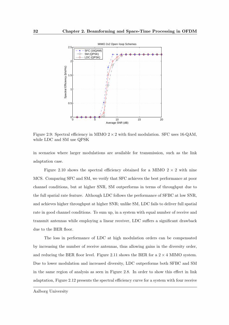
32 Chapter 2. Beamforming and Space-Time Processing in OFDM
0 5 10 15 200
0.5
1
1.5
2
2.5
Spe
ctra
l Effi
cien
cy (
b/s/
Hz)
Average SNR (dB)
MIMO 2x2 Open−loop Schemes
SFC (16QAM)SM (QPSK)LDC (QPSK)
Figure 2.9: Spectral efficiency in MIMO 2× 2 with fixed modulation. SFC uses 16-QAM,while LDC and SM use QPSK
in scenarios where larger modulations are available for transmission, such as the link
adaptation case.
Figure 2.10 shows the spectral efficiency obtained for a MIMO 2 × 2 with nine
MCS. Comparing SFC and SM, we verify that SFC achieves the best performance at poor
channel conditions, but at higher SNR, SM outperforms in terms of throughput due to
the full spatial rate feature. Although LDC follows the performance of SFBC at low SNR,
and achieves higher throughput at higher SNR; unlike SM, LDC fails to deliver full spatial
rate in good channel conditions. To sum up, in a system with equal number of receive and
transmit antennas while employing a linear receiver, LDC suffers a significant drawback
due to the BER floor.
The loss in performance of LDC at high modulation orders can be compensated
by increasing the number of receive antennas, thus allowing gains in the diversity order,
and reducing the BER floor level. Figure 2.11 shows the BER for a 2 × 4 MIMO system.
Due to lower modulation and increased diversity, LDC outperforms both SFBC and SM
in the same region of analysis as seen in Figure 2.8. In order to show this effect in link
adaptation, Figure 2.12 presents the spectral efficiency curve for a system with four receive
Aalborg University

2.3 MIMO and Rate Adaptation in OFDM 33
−10 −5 0 5 10 15 20 25 300
1
2
3
4
5
6
7
8
9
Spe
ctra
l Effi
cien
cy (
bps/
Hz)
Average SNR (dB)
MIMO 2x2 Open−loop Schemes: Link Adaptation
SFCSMLDC
Figure 2.10: Spectral efficiency in MIMO 2 × 2 with link adaptation
−10 −5 0 5 10 15 2010
−4
10−3
10−2
10−1
100
Unc
oded
BE
R
Average SNR (dB)
MIMO 2x4 Open−loop Schemes
SFC (16QAM)SM (QPSK)LDC (QPSK)
Figure 2.11: Probability of bit error of an uncoded system in MIMO 2 × 4 with fixedmodulation. SFC uses 16QAM, while LDC and SM use QPSK
Daniel Vaz Pato Figueiredo

34 Chapter 2. Beamforming and Space-Time Processing in OFDM
−10 −5 0 5 10 15 20 25 300
1
2
3
4
5
6
7
8
9
Spe
ctra
l Effi
cien
cy (
bps/
Hz)
Average SNR (dB)
MIMO 2x4 Open−loop Schemes: Link Adaptation
SFCSMLDC
Figure 2.12: Spectral efficiency in MIMO 2 × 4 with link adaptation
antennas. Although LDC now achieves the full spatial rate at high SNR, it still suffers a
loss compared to SM at high modulation orders.
2.3.4 Summary
This section evaluated the potential of LDC in a practical MIMO implementation. We
compared the spectral efficiency of different MIMO techniques and AMC in terms of diver-
sity and multiplexing. LDC increases the degrees of freedom to develop MIMO mapping
schemes aiming at multiplexing and diversity gains. However, with linear receivers these
designs have constraints that need to be evaluated. In particular, we compare the perfor-
mance of full rate LDC-UTOD with Alamouti and SM, under fair throughput conditions,
in order to assess the interaction between link adaptation and LDC. Results show that
UTOD is optimized for low modulation orders and higher number of receive antennas,
slightly outperforming the other schemes studied in low SNR conditions. Whereas for
dense modulations, SM outperforms UTOD at high SNR. Nevertheless, we show that an
increase in the number of receive antennas can dramatically improve the spectral efficiency
of the system in strong channel conditions.
Aalborg University

2.4 Conclusions 35
2.4 Conclusions
This chapter compared different approaches and gains of multiantenna techniques in
OFDM transmissions and combined them with link adaptation. Beamforming and spatial
diversity are designed for different channel characteristics and special issues need to be
considered when implementing each technique with OFDM.
Although LDC potentially provides higher gains with complex receivers, we combine
the full rate LDC code UTOD with a linear receiver to obtain a practical tradeoff between
spatial diversity and multiplexing. In this context, we show that UTOD, combined with
channel coding and AMC, proves to be a robust MIMO technique at low and mid-range
SNR, below 20 dB. However, the UTOD scheme only achieves the high SNR throughput
of SM by increasing the number of receivers in a MIMO configuration 2 × 4.
The link adaptation used in the second part of this chapter requires a CSI which
was considered to be error-free. In a practical scenario, however, the channel knowledge
obtained via feedback is not perfect. Chapter 3 focuses on the downlink adaptive trans-
mission of a MIMO spatial link for further investigation on the inaccuracy of feedback
channel information due to delay.
Daniel Vaz Pato Figueiredo


Chapter 3
Feedback Delay in Rate Adaptive
MIMO
Schemes that adapt the transmission parameters to the varying channel conditions increase
significantly the spectral efficiency of the channel. Particularly, rate adaptive systems pro-
vide substantial gains in performance with relatively low complexity, and reduced feedback
overhead [CEGHJ02, CG01].
In recent years, several authors have dedicated their research to analytical studies of
the performance of rate adaptive systems under feedback delay. Increasing the number of
bits in the modulated symbol boosts the data rate, thus it is wise to choose a more dense
modulation in favorable channel conditions. An adaptive multi-level QAM mechanism is
of interest for a system that adjusts the data rate based on CSI [AG00]. The recent surge
of interest in multiple antenna techniques rose the importance of studying the analytical
performance of adaptive M-QAM systems combined with STBC, as in [KT03], or SM, as
in [DB05].
Although rate adaptation provides performance gains in varying channel conditions,
the channel information required by this technique becomes outdated when the channel
is changing rapidly. A study on channel prediction and impact of outdated estimates in
time-varying channels is presented in [Goe99].
37

38 Chapter 3. Feedback Delay in Rate Adaptive MIMO
In scenarios where the feedback is subject to delays, channel prediction uses the
fading statistics to increase the reliability of the CSI. The authors in [Ekm02, Hol02]
derived closed-form approximations of the BER performance in SISO systems with a
power predictor.
This chapter studies the impact of feedback delay in discrete rate adaptation. We
obtain new closed-form analytical expressions for BER, and propose SNR switching thresh-
olds that take into account the channel uncertainty. Furthermore, we derive closed-form
expressions for the BER performance of the system for MIMO diversity and multiplexing,
as well as a tractable BER expression for AS.
The chapter is outlined as follows. Section 3.1 describes the system model and
evaluates the performance of rate adaptation combined with different antenna diversity
methods over Rayleigh channel through a statistical perspective. In the light of the feed-
back delay, Section 3.2 derives analytical performance measures to analyze the effect of
outdated channel information and proposes an approach to calculate switching thresholds
for the rate adaptive system. Section 3.3 analyzes the impact of channel prediction error
on the BER performance for MIMO diversity, multiplexing, and Antenna Selection (AS).
Section 3.4 shows the loss when the adaptation does not take into account the delay or
MIMO scheme employed for transmission. Finally, Section 3.5 presents the conclusions of
the chapter.
3.1 Link and System Implications from Outdated Feedback
This section describes the rate adaptive system for a multimode MIMO system over a
Rayleigh fading channel. This system is assumed in Sections 3.2, 3.3, and 3.4.
The system model in Figure 3.1 represents the link-level of the downlink of a cel-
lular system. The transmitter selects the QAM level to modulate data, as described in
Appendix E.1, and maps the symbols to the available antennas in the MIMO encoder.
The channel estimation is assumed to be perfect at the receiver. Then the terminal com-
municates the SNR in the CSI format via the feedback channel to the transmitter. On the
Aalborg University

3.1 Link and System Implications from Outdated Feedback 39
Adaptive M-QAM
MIMO encoder
Channel estimation
MIMO decoder
H
Demod
feedback
Figure 3.1: System model of MIMO and adaptive modulation
basis of the CSI, the system selects the rate, i.e., the constellation size of the modulation
to be transmitted.
The wireless channel is characterized by a flat Rayleigh fading channel. A different
number of antennas at transmitter and receiver ends is assumed according to the MIMO
configuration. The spatial links experience independent fading; thus, no correlation exists
between channel gains. The MIMO diversity mode considers STBC at the transmitter
and MRC at the receiver side. The SM mode employs a Zero Forcing (ZF) receiver to
decode the parallel streams, and the AS mode applies feedback information to choose the
proper transmit antenna.
As seen in Section 2.1, the narrowband linear model of the received signal is repre-
sented by
y = Hs + w ,
where H is the [Nr × Nt] matrix of complex Gaussian channel coefficients with variance
σ2h, s is the transmitted signal with energy Es, and w is the AWGN vector with power
N0.
For the SISO configuration, the CSI feedback is based on the SNR measured at
the receive antenna. However, due to the independency of the MIMO channels, the SNR
at each receive antenna provides insufficient information for the rate adaptation of the
transmission. The decision must be based on the post-processing SNR, i.e., after the
MIMO decoding, to account for the type of MIMO scheme. The post-SNR statistics of
the MIMO techniques are described in Appendix D.3.
Daniel Vaz Pato Figueiredo

40 Chapter 3. Feedback Delay in Rate Adaptive MIMO
The delay between the time that the MS measures the channel and the time that
the BS applies that information to send the signal in downlink is referred to as feedback
delay.
The rate adaptive scheme consists of a discrete M-QAM adaptation with a constant
transmit power and a BER constraint of BERt as described in Appendix E.1. In a practical
system, the SNR thresholds are found through measurements and building an extensive
look-up table, compensating for the effect of outdated CSI. However, this approach not
only increases the complexity of the system, but it also loses the generalization of the
model. This chapter aims at providing an analytical framework of the feedback delay
effect in Rayleigh fading channels. Therefore, we opt for analytical performance measures
to assess the degradation of the rate adaptive system combined with MIMO.
In order to reduce the uncertainty of the CSI in the presence of feedback delay,
Section 3.3 considers a prediction algorithm for the rate adaptive system. As detailed in
Appendix F.1, the predictor estimates the channel power within a time horizon based on
a regressor vector, i.e., a buffer with the observed past channel coefficients.
In the following, we present a preliminary evaluation of the outdated channel knowl-
edge received via feedback on different multiantenna techniques and multiuser scheduling.
3.1.1 Preliminary Evaluation of Outdated Channel
This section presents a preliminary study about the outdated CSI based on the time corre-
lation statistics. We evaluate the analytical throughput of a two level M-QAM adaptation
combined with different multiple antenna techniques over Rayleigh fading channel.
In a time-varying channel, the time correlation is a measure that describes the vari-
ation of the channel coefficients at time n and after a time delay of τ . As described in
Appendix A.2.1, when considering the Jakes model [JC94], the correlation between two
channel samples separated by a delay of τ is given by ρ = J0(2πfdτ), where fd is the
maximum Doppler frequency. One can calculate the distribution of the delayed channel,
hτ = h(n + τ), based on h = h(n). In [Goe99], the author shows that for a Rayleigh
Aalborg University

3.1 Link and System Implications from Outdated Feedback 41
channel, where the channel coefficients follow a complex Gaussian distribution with mean
µ and variance σ2, the delayed channel h(n+ τ)|h(n) also has a complex Gaussian distri-
bution with mean µ = ρh(n) and variance σ2 = 1− ρ2. In this preliminary approach, this
distribution is then used to generate the delayed channel coefficients available through
feedback, i.e., the value of the channel gain at the time n2 assuming that the channel
information available was measured at instant n1 = n2 − τ .
The rate adaptation module considers two M-QAM levels, namely QPSK and 16-
QAM, and the average SNR at the transmitter is 10 dB. The Rayleigh channel coefficients
are generated independently for each spatial link.
This link-level approach considers a single cell scenario and a point-to-point MIMO
link. The multiantenna techniques analyzed are STBC, AS, and MRC. The post-
processing SNR, defined by γ, is described for each considered MIMO scheme in Ap-
pendix D.3.
On the basis of the post-processing SNR, we compute analytically the spectral effi-
ciency of an uncoded M-QAM transmission and a packet size of Lp = 50 symbols, according
to η = log2(M)(1−BER(γ))Lp . As mentioned in Appendix B, the expression for uncoded
BER performance of square M-QAM with Gray bit mapping over AWGN is approximated
with [Pro01]
BER(M,γ) ≈ 2
log2M
(1 − 1√
M
)erfc
(√1.5
γ
M − 1
), (3.1)
where erfc(z) = 2√π
∫∞z e−t2dt.
A multiuser scheduler based on CSI is sensitive to the feedback delay. We use a max-
SNR scheduler that assigns the transmission to the user with the highest SNR at a given
slot, as described in Appendix E.2. Although the fast fading experienced by each user
is independent, we assume that all users have the same average SNR level, thus avoiding
fairness issues.
Based on the time length considered for frame duration, in the order of 1 ms, two
lengths for the feedback delay are considered, regular and fast feedback. The regular feed-
Daniel Vaz Pato Figueiredo
42 Chapter 3. Feedback Delay in Rate Adaptive MIMO
back channel suffers a delay within 0.5 and 1 ms, and is employed in the rate adaptation.
On the other hand, AS utilizes a fast feedback channel with delays between 0.1 and 0.5 ms.
Behind this assumption lies the fact that in the system perspective, it is not feasible to
change the modulation of a transmission within a shorter period than a frame duration,
since the receiver has to be aware of the change to decode the modulated symbols. On the
other hand, a change in the transmitting antenna can be done at the BS without the need
of informing the receiver; thus, it is transparent to the terminal and can be performed
faster.
3.1.1.1 Results
Results for a single-user system are presented in Figure 3.2. Figure 3.2(a) depicts the spec-
tral efficiency versus user mobility when ideal CSI is available at the BS, i.e., no feedback
delay. The user speed does not affect performance, since the delay is assumed instanta-
neous. As the results are statistical observations of the SNR distribution, the degradation
of STBC due to variation of the channel in consecutive symbols is not observed. The
scheme with two receivers implements MRC and achieves the highest performance, due
to the combination of array and diversity gains. The transmit diversity schemes with two
and four antennas apply STBC, and exploit diversity gain. AS scheme outperforms both
STBC configurations due to the gain obtained by the use of the feedback information.
Considering a fast feedback channel with 0.5 ms delay and a regular feedback of
1 ms, Figure 3.2(b) shows the degradation in performance due to an increase in speed
for the same multiantenna techniques. In fact, at higher speed, the channel becomes
more time-variant, and the probability of choosing a modulation not appropriate for the
channel quality increases. In this case, we observe a stronger effect of mobility in the AS
scheme due to its sensitivity to feedback delays, and the transmit diversity as more robust
technique.
Figure 3.3 shows the spectral efficiency of a system with ten users at the same av-
erage SNR of 10 dB. It is significant to note that when the delay is low, Figure 3.3(a)
Aalborg University

3.1 Link and System Implications from Outdated Feedback 43
0 50 100 150 2001
1.1
1.2
1.3
1.4
1.5
1.6
1.7
1.8
1.9
SISO
Tx Div: 2x1
Tx Div: 4x1
Rx Div: 1x2
Tx AS: 2
Sp
ectr
al E
ffic
ien
cy
Speed (kmph)
(a) no delay feedback (ideal)
0 20 40 60 80 1000.9
1
1.1
1.2
1.3
1.4
1.5
1.6
1.7
1.8
1.9
SISO
Tx Div: 2x1
Tx Div: 4x1
Rx Div: 1x2
Tx AS: 2
Sp
ectr
al E
ffic
ien
cy
Speed (kmph)
(b) fast feedback: 0.5 ms, regular feedback: 1 ms
Figure 3.2: Single-user scenario
0 20 40 60 80 1001
1.2
1.4
1.6
1.8
2
2.2
2.4
2.6
2.8
3
SISO
Tx Div: 2x1
Tx Div: 4x1
Rx Div: 1x2
Tx AS: 2
Speed (kmph)
Sp
ectr
al E
ffic
ien
cy
(a) fast feedback: 0.1 ms, regular feedback: 0.5 ms
0 20 40 60 80 1000.5
1
1.5
2
2.5
3
SISO
Tx Div: 2x1
Tx Div: 4x1
Rx Div: 1x2
Tx AS: 2
Sp
ectr
al E
ffic
ien
cy
Speed (kmph)
(b) fast feedback: 0.5 ms, regular feedback: 1 ms
Figure 3.3: Ten users scenario with scheduler max-SNR
shows that the MUD gain available at low speed is higher for a SISO configuration than
for transmit diversity. This effect is explained by an incompatibility of diversity tech-
niques, i.e., the scheduler provides no benefit in a constant channel. In other words, the
MUD gain is significantly diminished when combined with spatial diversity. In fact, while
the opportunistic scheduling exploits the channel variability allocating users at peaks
of channel power, STBC introduces channel hardening, i.e., reduces the range of the
SNR [HMT04, BKRM+03]. However, when feedback delays are considered in the system
and the speed increases, the scheduler and AS lose part of their gain, due to outdated
feedback, as depicted in Figure 3.3(b).
Daniel Vaz Pato Figueiredo

44 Chapter 3. Feedback Delay in Rate Adaptive MIMO
3.1.2 Summary
Closed-loop schemes provide performance gains in low mobility scenarios, but suffer degra-
dation due to feedback delay as the speed of the terminal increases. Although open-loop
spatial diversity proves to be incompatible with multiuser scheduling, it makes the system
more robust at high mobility.
The selection of MIMO techniques in systems on the basis of CSI obtained via
feedback must consider the variability of the channel. Hence, next sections derive and
look into the analytical expressions of the performance of adaptive rate schemes with
MIMO.
3.2 Analytical Performance of Rate Adaptation
This section describes and derives the analytical expressions for the BER and throughput
of the rate adaptation mechanism combined with spatial diversity.
The expression (3.1), for the uncoded BER, is not easily invertible. Therefore, as
described in Appendix E.1, the up-coming derivations we use the approximation proposed
in [CG01]:
BER(M,γ) ≈ 0.2 exp
(−1.6γ
M − 1
). (3.2)
This approximation is shown in [CG01] to be tight within 1 dB for BER ≤ 10−3 and
M ≥ 4.
The system emplys an adaptive discrete modulation, i.e., M is restricted to 2i,
where i is an integer, adapted by the system according to the measured γ. Moreover, the
power at the transmitter is kept constant and not adapted. It has been shown in [CG01]
that the adaptation of both rate and power does not bring significant advantage over the
adaptation of only rate.
In this adaptive scheme, for R available constellation sizes, the SNR is divided into
R + 1 regions. The Mi order of QAM is transmitted once the SNR falls into region i
delimited by SNR thresholds (or switching thresholds). To define the SNR thresholds,
Aalborg University

3.2 Analytical Performance of Rate Adaptation 45
we apply an instantaneous BER constraint, such that the BER is always smaller than a
target value, i.e., BER ≤ BERt; thus obtaining the SNR threshold γi for region i,
γi =Mi − 1
−1.6ln
(BERt
0.2
). (3.3)
In the discrete adaptive M-QAM system, the average BER within one SNR region
i is obtained by averaging (3.2) over the SNR distribution. The average BER is repre-
sented by the sum of the BER of each region weighted with the number of bits of the
modulation [AG00] as follows:
BER =
∑Ri=0 log2(Mi)
∫ γi+1
γiBER(Mi, γ)f(γ)dγ
∑Ri=0 log2(Mi)
∫ γi+1
γif(γ)dγ
. (3.4)
Given this adaptive modulation scheme, the average spectral efficiency is given by
the probability that the SNR lies within the boundaries of each fading region and takes
into account the errors on the link; thus, for an uncoded system, it is given by
ηeff =
R−1∑
i=0
log2(Mi)
∫ γi+1
γi
f(γ)dγ
(1 − log2(Mi)
∫ γi+1
γi
BER(γ)f(γ)dγ
). (3.5)
When the value of SNR used to adapt the transmission at the BS contains an error,
the predicted SNR, γ, is different from the true SNR experienced, γ, thus the approximated
BER can be re-written as
BER(γ, γ) = BER(Mi, γ) ≈ 0.2 exp
( −1.6γ
Mi(γ) − 1
).
Note that the order Mi(γ) is adapted on the basis of the predicted SNR at the BS, γ.
However, in the notation, we will drop this dependence and use hereon only Mi. The
instantaneous BER of the system as a function of γ is
BER(γ) =
∫ ∞
0BER(γ, γ)f(γ|γ) dγ , (3.6)
Daniel Vaz Pato Figueiredo

46 Chapter 3. Feedback Delay in Rate Adaptive MIMO
and new SNR thresholds have to be computed for the system to meet the BER constraint.
In an adaptive rate system based on predicted values of the SNR, the average BER
for discrete rate adaptation with R constellations and the average spectral efficiency are
BER =
∑R−1i=0 log2(Mi)
∫ γi+1
γiBER(γ)f(γ)dγ
∑R−1i=0 log2(Mi)
∫ γi+1
γif(γ)dγ
, (3.7)
ηeff =R−1∑
i=0
log2(Mi)
∫ γi+1
γi
f(γ)dγ
(1 − log2(Mi)
∫ γi+1
γi
BER(γ)f(γ)dγ
). (3.8)
3.2.1 Evaluation of Analytical Performance
This section details the closed-form expressions of the BER performance analytical mea-
sures for rate adaptation in the context of MIMO diversity. Assuming no feedback delay,
Section 3.2.1.1 deals with the instantaneous BER approximation in (3.2) and the thresh-
olds in (3.3). Section 3.2.1.2 analyzes the case with feedback delay applying the BER
definition of (3.6).
3.2.1.1 Analytical Measures for Ideal Feedback
In the context of the statistics of the MIMO diversity channel as described in Appendix D.3.1,
we derive closed-form expressions of the average performance measures for MIMO diversity
scheme with rate adaptation.
As used in [AG00], the probability of ith fading region in a Rayleigh channel can be
expressed as follows:
∫ γi+1
γi
f(γ)dγ =Γ(NtNr,
Nt
γ γi) − Γ(NtNr,Nt
γ γi+1)
Γ(NtNr), (3.9)
where Γ(.) is the complete gamma function, and Γ(., .) is the incomplete gamma function.
From this closed-form expression, we obtain the average spectral efficiency, applying (3.5),
of the adaptive rate system shown in Section 3.2.1.1.
The average BER within a single fading region can be expressed for MIMO diversity
Aalborg University

3.2 Analytical Performance of Rate Adaptation 47
scheme as
BERi =
∫ γi+1
γi
BER(Mi, γ)f(γ)dγ
= 0.2
(Nt
γ
1
bi
)NtNr Γ(NtNr, biγi) − Γ(NtNr, biγi+1)
Γ(NtNr), (3.10)
where bi = Nt
γ + 1.6Mi−1 . Using (3.9) and (3.10) in (3.4), one can derive the average BER of
the adaptive rate system.
The thresholds defined by (3.3) are addressed to as generic thresholds. These thresh-
olds assume an instantaneous delay-free feedback situation, i.e., no delay is taken into
account in the SNR thresholds design.
3.2.1.2 Analytical Measures for Delayed Feedback
In this section, we introduce a delay τ between the time the SNR is measured and the
time it is employed at transmitter, and derive closed-form expressions of the average
performance measures for MIMO diversity scheme with rate adaptation.
It should be noted that the time delay, τ , of the feedback in a time-varying channel
affects the BER performance, but not the attempted throughput. For a signal transmitted
at instant n, with channel SNR, γn, the decision about the modulation size is taken at
instant n− τ , i.e., the adaptation is performed based on γn−τ . As no prediction algorithm
is assumed here, the prediction SNR is the outdated SNR, γ = γn−τ .
Consider γ and γ, as the SNR at instants n and n − τ , respectively. Then, for
a MIMO diversity link, it is possible to prove that the conditional Probability Density
Function (PDF) of γ given γ is
f(γ|γ) =Nt
(1 − ρ)γ(γ)
NtNr−12 (ργ)−
NtNr−12 exp
(−Nt(ργ + γ)
(1 − ρ)γ
)
× INtNr−1
(2Nt
√ρ
(1 − ρ)γ
√γγ
),
where, assuming Jakes model for time variation, the time correlation factor is ρ = J20 (2πfdτ),
Daniel Vaz Pato Figueiredo

48 Chapter 3. Feedback Delay in Rate Adaptive MIMO
and Iβ(z) is the modified Bessel function of order β.
With the knowledge of the conditional PDF of the SNR, the instantaneous BER
based on the delayed SNR in (3.6) is
BER(γ) =
∫ ∞
0BER(γ, γ)f(γ|γ)dγ
= 0.2
(1
1 + 1.6Mi−1
γ(1−ρ)Nt
)NtNr
exp
(γρ 1.6
Mi−1
1 + 1.6Mi−1
γ(1−ρ)Nt
). (3.11)
In this case, the generic thresholds shown in (3.3) are not accurate; thus, introducing
updated thresholds that consider feedback delay is necessary for a correct selection of rate.
The updated thresholds are obtained by inverting the equation (3.11), and can be written
as
γi =1 + 1.6
Mi−1γ(1−ρ)
Nt
ρ 1.6Mi−1
ln
[5BERt
(1 +
1.6
Mi − 1
γ(1 − ρ)
Nt
)NtNr
]. (3.12)
Similar to (3.10), the closed-form expression for the average BER within fading
region i reads
BERρi =
∫ γi+1
γi
BER(γ)f(γ)dγ
= 0.2
(Nt
γbi
)NtNr Γ(NtNr, bρi γi) − Γ(NtNr, b
ρi γi+1)
Γ(NtNr),
where bρi = Nt
γ + 1.6Ntρ1.6(1−ρ)+Nt(Mi−1) .
3.2.2 Results and Discussion
This section presents the results for an adaptive M-QAM system with constellation sizes
M = 4, 16, 64, 256, and with BERt = 10−3. The receiver tracks continuously the post-
processing SNR, and the M-QAM order is computed based on the SNR thresholds.
Figure 3.4 depicts the analytical curves of the average BER performance of a delay-
free SISO and MRC system. Notice that the average BER is always below BERt, due
to the instantaneous constraint BER ≤ BERt. In the same plot, the simulation curves
Aalborg University

3.2 Analytical Performance of Rate Adaptation 49
0 5 10 15 20 25 30 35 40
10−4
10−3
10−2
Average SNR (dB)
Ave
rage
BE
R
Adaptive M−QAM over Rayleigh Fading Channel
SISOMRCSISO simMRC sim
Figure 3.4: Average BER of a discrete M-QAM adaptive system. The lines without markerrepresent the analytical results, whereas the star corresponds to the simulation results forthe case with no feedback delay
for the situation without feedback delay are plotted. The difference between analytical
and simulated curves resides in the fact that the BER approximation is not exact and the
inaccuracy increases in adaptive rate system for higher modulation orders.
The performance of the system in the presence of feedback delay is shown to be
affected by the use of generic thresholds (3.3) or updated thresholds (3.12). In fact,
Figure 3.5 shows that the BER degradation is significant when generic thresholds are used
with a normalized time delay experienced by the feedback of fdτ = 0.06. In SISO with
generic thresholds, the BER constraint is not fulfilled for a long range of channel conditions
(15 ≤ γ ≤ 38 dB), whereas the updated thresholds maintain the BER performance under
the required BER constraint. Also for MRC scheme, which is generally more robust, the
average BER performance is improved by employing the updated thresholds.
3.2.3 Summary
This section evaluated the performance of a rate adaptive system combined with spatial
diversity in a time-variant channel. Closed-form expressions of the BER were derived
Daniel Vaz Pato Figueiredo

50 Chapter 3. Feedback Delay in Rate Adaptive MIMO
0 5 10 15 20 25 30 35 4010
−5
10−4
10−3
10−2
Average SNR (dB)
Ave
rage
BE
R
Adaptive M−QAM over Rayleigh Fading Channel
SISO genMRC genSISO updMRC upd
Figure 3.5: Average BER of a discrete M-QAM adaptive system with delay. Normalizedfeedback delay is fdτ = 0.06. The star corresponds to generic and the diamond to updatedthresholds
for a M-QAM scheme with spatial diversity over flat Rayleigh fading channels and with
feedback delay. More conservative thresholds that take into account the feedback delay
were derived, and compared with generic thresholds.
3.3 Channel Power Prediction
Section 3.2 showed the impact of feedback delay in the rate adaptation performance.
However, prediction methods have been proposed to reduce the uncertainty of the CSI
obtained via feedback in time-variant channels. This section presents the analytical study
on the BER performance of an adaptive M-QAM with channel power prediction for various
MIMO schemes.
On the basis of the power predictor proposed in [Ekm02], this section derives new
closed-form expressions for the BER performance of different MIMO schemes. Analytical
SNR thresholds are then obtained from the closed-form expressions.
Aalborg University

3.3 Channel Power Prediction 51
3.3.1 Power Prediction
In [Ekm02, ESA02], a prediction based on linear regression is analyzed in the context
of a Rayleigh fading channel. The predictor is detailed in Appendix F.1. The channel
coefficients are predicted L symbols ahead using a regressor vector and Mean Square
Error (MSE) optimal weights. On the basis of the prediction of coefficients, h, the unbiased
power predictor was shown to be
pn|n−L = |hn|n−L|2 + σ2ǫh
.
The prediction of the instantaneous SNR is then obtained from the predicted power
with γ = pEs
N0.
3.3.2 MIMO Diversity
Appendix F.2 shows the derivation of the distribution functions of the SNR, and Ap-
pendix F.3 the closed-form expressions for the BER performance. The main results are
presented for MIMO diversity. The PDF of the SNR conditioned on the predicted SNR
for a MIMO diversity scheme, (F.16), is
f(γ|γ) = U(γ)U(γ −Nrγυhǫh)Nt
γυhǫh
γNtNr−1
2 (γ −Nrγυhǫh)−NtNt−1
2
× exp
[−γ + γ −Nrγυhǫh
γNrυhǫh
]INtNr−1
(2Nt
γυhǫh
√γ(γ −Nrγυhǫh)
),
where υhǫh is the relative prediction error variance, and includes the effect of both the
feedback delay and the prediction error.
Daniel Vaz Pato Figueiredo

52 Chapter 3. Feedback Delay in Rate Adaptive MIMO
The instantaneous BER as a function of γ, (F.24), is obtained as follows:
BER(γ) =
∫ ∞
0BER(γ, γ)f(γ|γ)dγ
= U(γ −Nrγυhǫh)0.2
(Nt
γυhǫhb(i)
)NtNr
exp
[γ −Nrγυhǫh
γNtυhǫh
(Nt
γυhǫhb(i)− 1
)],
(3.13)
where b(i) = Nt
γυhǫh
+ 1.6Mi−1 .
The generic SNR thresholds in (3.3) are applicable when the feedback is assumed
delay-free, i.e., a constant channel in the window of time where the adaptation takes
place. When the channel is time-variant, the feedback delay introduces a level of uncer-
tainty in the information of the channel quality. The updated SNR thresholds take into
account both the relative prediction error variance and the receiver combining technique
to compensate the mismatch.
For a system with instantaneous BER constraint BER ≤ BERt, and constant trans-
mit power, the updated SNR thresholds, (F.25), are given by
γi = Nrγυhǫh +γυhǫh
Nt
(Nt
γυhǫh
b(i) − 1) ln
[BERt
0.2
(γυhǫhb(i)
Nt
)NtNr
]. (3.14)
3.3.3 MIMO Multiplexing
Similar to the previous section, Appendix F.2 shows the derivation of the distribution func-
tions of the SNR, and Appendix F.3 the closed-form expressions for the BER performance.
The PDF of the SNR conditioned on the predicted SNR for SM, (F.9), is
f(γ|γ) =U(γ)U(γ − γυhǫh)
γNaυhǫh
exp
[−γ + γ − γυhǫh
γNaυhǫh
]I0
(2Na
γυhǫh
√γ(γ − γυhǫh)
).
Aalborg University

3.3 Channel Power Prediction 53
The instantaneous BER as a function of γ, (F.22), is obtained as follows:
BER(γ) =
∫ ∞
0BER(γ, γ)f(γ|γ)dγ
= U(γ − γυhǫh)0.2Na
γυhǫhb(i)exp
[γ − γυhǫh
γNa
(Na
γυhǫhb(i)− 1
)], (3.15)
where b(i) = Na
γυhǫh
+ 1.6Mi−1 .
Finally, as opposed to the generic thresholds in (3.3), the updated SNR thresholds
for SM, (F.23), are given by
γi = γυhǫh +γυhǫh
Na
(Na
γυhǫh
b(i) − 1) ln
[BERt
0.2
γυhǫhb(i)
Na
]. (3.16)
3.3.4 Antenna Selection
For AS, the expression obtained for conditional PDF of the SNR is presented in Ap-
pendix F.2 and the BER in Appendix F.3, but no closed-form is found for the updated
thresholds. Nevertheless, the tractable equation for the BER performance allows for a
numerical evaluation.
3.3.5 Evaluation of Analytical Performance
In order to plot the analytical curves of BER and average effective throughput, the system
described in Section 3.1 is assumed with four M-QAM levels and an unbiased power
predictor. The instantaneous BER curves in AWGN channel, expressed by (3.2), for the
four M-QAM levels using SISO in a delay-free scenario are depicted in Figure 3.6. In the
discrete rate adaptive system, the region of interest in the curves is below the target BER.
The average BER, expressed by (3.4), depends on the fading channel assumed. To
obtain a Rayleigh channel performance, the average BER is computed over 106 symbols for
each SNR value. The link experiences a constant channel realization within each symbol.
We have chosen a target BER of 10−3, thus the system uses the largest modulation that has
Daniel Vaz Pato Figueiredo

54 Chapter 3. Feedback Delay in Rate Adaptive MIMO
−10 −5 0 5 10 15 20 25 3010
−10
10−8
10−6
10−4
10−2
100
BE
R
SNR predicted (dB)
4 QAM16 QAM64 QAM256 QAM
Figure 3.6: BER for different M-QAM levels
a BER below 10−3. Figure 3.7 depicts the average BER, for the adaptive M-QAM without
feedback delay applied to SISO, STBC, MRC, and SM. The AS scheme is not represented
in these results, since no closed-form of the instantaneous BER was obtained. Note that
the average BER is always below the instantaneous constraint, i.e., BER ≤ BERt, and
the diversity and array gains are visible at higher SNR values.
In the presence of feedback delay, the instantaneous BER expression assumes the
form of (3.13) for MIMO diversity and (3.15) for MIMO spatial multiplexing. In a SISO
system, Figure 3.8 depicts the instantaneous BER in terms of predicted SNR for QPSK
and increasing relative prediction error variance, υhǫh . The prediction error variance is
affected by the prediction horizon and the time variance of the channel. Thus, in a delay-
free feedback scenario, or in a time constant channel, the prediction error variance tends
to zero. Due to this effect, the SNR thresholds, valid in the delay-free case, fail at high
prediction error and need to be updated according to the new BER curve, as Figure 3.8
illustrates.
Evaluating (3.13) and (3.15) for configurations with more than one antenna, Fig-
ures 3.9(a) and 3.9(b) show the analytical curves for the MIMO techniques under consid-
Aalborg University

3.3 Channel Power Prediction 55
0 5 10 15 20 25 30 35 4010
−6
10−5
10−4
10−3
Average SNR (dB)
Ave
rage
BE
R
Adaptive M−QAM over Rayleigh fading channel − Analytical
SISO (1x1)MRC (1x2)STBC (2x1)SM (2x2)
Figure 3.7: Adaptive M-QAM (M=0,4,16,64,256) over Rayleigh fading channel. BERt =10−3
−10 −5 0 5 10 15 20 25 3010
−10
10−8
10−6
10−4
10−2
100
BE
R
SNR predicted (dB)
ve=1e−5ve=1e−2ve=1e−1
Figure 3.8: BER curves of SISO for different values of relative error variance. Using QPSKand γ = 20 dB
Daniel Vaz Pato Figueiredo

56 Chapter 3. Feedback Delay in Rate Adaptive MIMO
−20 −15 −10 −5 0 5 10 15 2010
−10
10−8
10−6
10−4
10−2
100
SNR predicted (dB)
BE
R
SISOSIMOMISOMIMO−STBC−MRCMIMO−SM−ZF
(a) low prediction error variance (υhǫh = 10−4)
2 4 6 8 10 12 14 16 18 2010
−10
10−8
10−6
10−4
10−2
100
SNR predicted (dB)
BE
R
SISOSIMOMISOMIMO−STBC−MRCMIMO−SM−ZF
(b) high prediction error variance (υhǫh = 10−2)
Figure 3.9: BER curves for different MIMO techniques. Using QPSK and γ = 20 dB
eration for two cases of prediction error, low relative prediction error variance and high
prediction error variance, respectively. While all MIMO modes follow the same instan-
taneous BER performance in an error-free CSI scenario, as shown in Figure 3.9(a), the
differences appear at higher prediction error variance, and are more evident in MIMO
diversity configuration.
The average BER in the case with prediction error is obtained by using the instan-
taneous BER, (3.13) and (3.15), in (3.4). Figure 3.10 shows the average BER curve for
the discrete SNR, when delay is considered for different MIMO schemes. The degradation
in performance is more significant for values of relative prediction error of υhǫh ≥ 10−1.
Figure 3.11 depicts the average effective throughput for the same set of schemes. In
the case of a higher prediction error, the performance degradation is significant, and the
trend is more evident and pronounced in the case of SISO and SM schemes.
3.3.6 Summary
In this section, we presented closed-form expressions for the BER performance of MIMO
diversity and SM techniques when a rate adaptive system employs a predictor for the
SNR. Although for AS no closed-form of the BER was achieved, a tractable expression
was derived, which permits a numerical analysis of performance to be applied in Chapter 4.
The feedback delay and the prediction error were shown to have different impact on the
Aalborg University

3.3 Channel Power Prediction 57
10−4
10−3
10−2
10−1
100
10−4
10−3
relative predictor error variance
Ave
rage
BE
RSISOMRCSTBCSM
Figure 3.10: Average BER for different MIMO techniques. γ = 20 dB and BERt = 10−3
10−4
10−3
10−2
10−1
100
1
2
3
4
5
6
7
relative predictor error variance
Spe
ctra
l effi
cien
cy
SISOMRCSTBCSM
Figure 3.11: Average effective throughput for different MIMO techniques. γ = 20 dB andBERt = 10−3
Daniel Vaz Pato Figueiredo

58 Chapter 3. Feedback Delay in Rate Adaptive MIMO
instantaneous BER of each MIMO scheme.
3.4 Practical System Aspects
The SNR thresholds for rate selection depend on the SNR distribution of the MIMO trans-
mission scheme as well as on the number of antennas. Moreover, in the presence of feedback
delay, the SNR thresholds also depend on the relative prediction error variance, υhǫh .
The results presented so far assume that the SNR thresholds of the system are
updated according to the prediction error and the MIMO technique. However, since
these thresholds require a higher complexity in the system to obtain the estimate of the
prediction error variance, a simpler version of a rate adaptive system would use generic
thresholds (not updated). The generic thresholds can also be applied when the information
about the channel variability is unknown, or when the feedback message does not allow
to include information about the MIMO scheme and the prediction error variance. This
section shows the degradation that arises from SNR thresholds that are not updated (or
updated incorrectly) to the channel conditions.
The SNR thresholds with incorrect values are analyzed for two parameters: trans-
mission technique and value of prediction error variance. This work identifies two plausible
situations that occur in a simplified rate adaptive system. The system uses a feedback
message with the SNR measured in the symbol received, but neither the MIMO mode
nor the prediction error variance are taken into account. The first case applies SISO
thresholds for any MIMO technique, and is presented in Section 3.4.1. The second case
considers generic thresholds (not considering delay effect) instead of updated thresholds,
and is presented in Section 3.4.2.
3.4.1 SISO thresholds for MIMO
When the rate adaptation system is unaware of the different multiple antenna techniques,
the system assumes a SISO link. Figure 3.12 depicts the loss in throughput for other
MIMO techniques. The results show that the use of SISO thresholds for other MIMO
Aalborg University

3.4 Practical System Aspects 59
10−4
10−3
10−2
10−1
100
0
1
2
3
4
5
6
7
relative predictor error variance
Spe
ctra
l effi
cien
cy
SISOMRCSTBCSMMRC−SISO thrSTBC−SISO thrSM−SISO thr
Figure 3.12: Average effective throughput for different MIMO techniques. Updated versusSISO thresholds. γ = 20 dB and BERt = 10−3. The ’solid lines’ represent the updatedthresholds, and the ’dotted lines’ represent the SISO thresholds
configurations creates a substantial loss in performance, but the effect is very different
depending on the technique. The SM scheme reveals to be more sensitive to prediction
error when compared to the diversity schemes. More specifically, even at υhǫh ≤ 10−2,
the performance loss is significant. On the other hand, MRC has an almost negligible
degradation in performance.
3.4.2 Generic versus Updated Thresholds
In previous sections, two types of SNR thresholds, the generic and the updated thresh-
olds, were defined. While the generic thresholds do not take into account the delay and
prediction errors, the updated thresholds consider the statistics of the predicted SNR ac-
cordingly. Here, we analyze the impact of the generic thresholds that are not updated
with the prediction error. The system suffers a delay in the feedback between receiver and
transmitter, but the thresholds assume zero delay feedback.
Figure 3.13 depicts the loss in BER performance against the relative predictor error
variance. Updated thresholds are more conservative, as these compensate the uncertainty
Daniel Vaz Pato Figueiredo

60 Chapter 3. Feedback Delay in Rate Adaptive MIMO
10−4
10−3
10−2
10−1
100
10−4
10−3
10−2
relative predictor error variance
Ave
rage
BE
R
SISOMRCSTBCSMSISO−not updMRC−not updSTBC−not updSM−not upd
Figure 3.13: Average BER for MIMO techniques. Updated versus generic thresholds.γ = 20 dB and BERt = 10−3. The ’solid lines’ represent the updated thresholds, and the’dotted lines’ represent the generic thresholds
in the feedback CSI by increasing the SNR threshold. However, while the difference of
performance in SISO and SM is substantial, MRC and STBC updated thresholds have
lower impact in the BER. In fact, the BER for SISO and SM is only kept under the
constraint if updated thresholds are used, confirming these schemes as the less robust
techniques to prediction errors.
3.4.3 Summary
This section presented the analysis of the effect of the prediction error in the CSI obtained
with a feedback channel that experiences delay. We have separately studied the case of
updated SNR thresholds that do not take the MIMO mode into account, as well as the
case of updated SNR thresholds that do not consider the delay.
Aalborg University

3.5 Conclusions 61
3.5 Conclusions
This chapter addressed the impact of feedback delay in the performance of adaptive sys-
tems. The goal was to find the extent to which a system affected by delay can be tuned
while meeting the BER constraints.
The statistics of the post-processing SNR can be used to evaluate the effect of
feedback delay, as well as they can be used to design SNR thresholds. To assess the
sensitivity of different multiantenna techniques under a time-variant channel, we have
studied the average BER over flat Rayleigh fading channels.
The channel prediction reduces the uncertainty of channel information at transmitter
caused by feedback delay. In addition, with an unbiased channel power predictor, we have
identified a measure for the reliability of the CSI in feedback directly related with the
normalized delay and the predictor regressor.
On the basis of the analytical study, this chapter presented closed-form expressions
for the BER of MIMO diversity and SM, and it also proposed SNR thresholds updated
according to the CSI inaccuracy due to delay. Simulation results show that these thresholds
fulfill the BER constraint in the presence of delayed feedback.
The feedback delay and the time variability of the channel are factors that need to
be considered both in the design of a rate adaptive system and in the choice of MIMO.
The selection of the best scheme according to the channel conditions and feedback delay
is determinant for receivers that are able to use different MIMO modes. These results are
applied in Chapter 4 to propose such MIMO switching mechanism.
Daniel Vaz Pato Figueiredo


Chapter 4
Adaptive MIMO-OFDMA
Mechanisms
The reliability of the CSI available at the transmitter is a determinant factor in a link
adaptation system based on feedback. In Chapter 3, we derived new thresholds for a rate
adaptive scheme. These thresholds take into account the channel prediction error variance
and the MIMO technique. On the basis of that background, this chapter presents a general
framework of a system with multiple MIMO capabilities. In addition, we aim at tackling
some of the more practical issues for implementation in a multiuser system. As a result,
the present chapter proposes a transmit strategy for a multimode MIMO system with a
generic OFDMA allocation, and focuses on the choice of MIMO modes in an integrated
MIMO switching system.
The previous chapters showed how different MIMO techniques provide various per-
formance benefits, e.g., robustness and throughput. Several authors have addressed the
MIMO adaptation issue in recent years, such as switching mechanisms between spatial
diversity and multiplexing based on the SNR, the MIMO channel eigenvalues, and the
condition number of the spatial correlation matrix [HJP05, WSKM06, FPKHJ05]. How-
ever, to the author’s knowledge, schemes incorporating the reliability of CSI feedback of
the MS have not been proposed to date. Moreover, the combination of multiuser alloca-
63

64 Chapter 4. Adaptive MIMO-OFDMA Mechanisms
tion of subchannels in OFDM with multimode MIMO selection reveals to be a practical
approach for integrated systems. In [MKL06], the authors present an integrated alloca-
tion scheme for the transmission parameters of real-time and non real-time services to the
users in the cell center or the cell-edge. This chapter proposes a concept for an integrated
system based on the reliability of the CSI.
The remainder of this chapter is organized as follows. Section 4.1 describes the
general system structure and presents a preliminary evaluation of feedback delay and
SNR thresholds in a simplified link adaptation system. Section 4.2 proposes the strategy
for the switching mechanism to optimize the performance of the feedback in the presence
of delay, and it proposes a MIMO look-up table for two transmit antennas. Based on
the different approach required for frame-based communications, Section 4.3 presents an
analysis of different options for setting the thresholds in this case and proposes a tradeoff
solution. Finally, Section 4.4 points out the main conclusions of the chapter.
4.1 System Description
This section presents the structure of the general framework for an OFDM-based system
with MIMO and link adaptation capabilities. We consider the downlink of a single cell
OFDMA system with carrier frequency at 2 GHz. The BS possesses two or more antennas
and can switch between different transmit modes. Moreover, the BS schedules the users
by allocating the available subchannels, based on CSI sent via a feedback channel from the
MS. As the users are given different subcarriers, we consider that there is no inter-user
interference at the receiver.
The wireless channel is frequency selective over the system bandwidth, but the sim-
ulations consider the performance of a flat fading single OFDM subcarrier. The channel is
quasi-static varying in time according to the classical Doppler, such that it is approximately
constant over two consecutive symbols. The spatial links of the MIMO configuration are
uncorrelated, and a limited signalling overhead is considered for the feedback channel.
Based on these conditions, the MIMO transmission modes selected for analysis were the
Aalborg University

4.1 System Description 65
Adaptive M-QAM
MIMO encoder
Channel estimation
MIMO decoder
H
Demod
feedback
Figure 4.1: System model of MIMO and adaptive modulation
single antenna (SISO), the open-loop schemes STBC and SM, and the closed-loop AS.
Following the analytical study of Chapter 3, we consider a simple ZF detector for SM.
The average transmit energy is assumed the same for all MIMO options.
The BS supports a rate adaptation system that selects the current modulation for
each user in the downlink frame on the basis of feedback CSI. The available constellations
are QPSK, 16-QAM, 64-QAM, and 256-QAM. The system model of a channel allocated
to one user is represented in Figure 4.1.
The channel estimation at the MS is assumed perfect. The MS tracks the channel
quality on its allocated subchannels and sends the feedback information on an uplink
channel to the BS. The tracking process is performed on one antenna when AS mode is
selected for transmission or over the two transmit antennas for STBC or SM.
The delay between the channel measure at MS and the frame transmitted from
BS adapted according to the CSI is the feedback delay, τ . The normalized value of
feedback delay is fdτ . The BS tracks the channel time variability by means of stored past
information in a CSI buffer, and uses it to determine the reliability measure of the link.
Channel prediction is embedded at the MS to compensate for the time variability of the
channel. On the basis of the prediction error variance, the BS selects the appropriate
transmission mode. The SNR thresholds derived in Chapter 3 are implemented to select
the rate by taking into account the MIMO mode and the prediction error.
The BS schedules the transmission to different users based on the CSI sent via
feedback. The decision on the subchannel and transmit strategy allocated to each MS
is performed before transmission of every downlink frame. The implications of reporting
Daniel Vaz Pato Figueiredo

66 Chapter 4. Adaptive MIMO-OFDMA Mechanisms
L O C
c h
a n n e
l s
D I V
c h a
n n e
l s
...
L O C
c h
a n n e
l s
D I V
c h a
n n e
l s
time
f r e q
u e n
c y
channel 1 channel 1
channel 2 channel 2
Figure 4.2: LOC and DIV subchannels within an OFDM frame
the CSI on a frame basis are analyzed in Section 4.3. The simulation results prior to
Section 4.3 assume a rate adaptation on a symbol by symbol basis.
The OFDM data subcarriers are grouped to form subchannels that are allocated
to the users in the system. One subchannel consists of a number of subcarriers that
can be contiguous or not. In this context, the terms Localized (LOC) and Diversity
(DIV) subchannels are employed to refer to the two types of aggregated subcarriers in the
OFDMA system. LOC subchannels consist of contiguous subcarriers. DIV subchannels
consist of non-contiguous subcarriers that are ideally separated (in frequency) by at least
the coherence bandwidth to provide inherent diversity. Within a LOC subchannel, the
SNR is assumed constant over the subcarriers; thus, it is suitable for rate adaptation
across different LOC subchannels. The DIV subchannels are appropriate for application
of frequency diversity coding. Figure 4.2 depicts the frame structure containing both LOC
and DIV channels. The MS estimates the SNRs of each spatial link for both LOC and
DIV channels.
4.1.1 Performance of MIMO Modes with Outdated Feedback
This section evaluates the performance of different MIMO techniques facing outdated
feedback CSI. The results of this analysis are applied in the choice of the MIMO modes
Aalborg University

4.1 System Description 67
0 5 10 15 20 25 30 35 400
2
4
6
8
10
12
14
16
Average SNR (dB)
Goo
dput
Adaptive M−QAM over Rayleigh Fading Channel
SISOASMRCAS−MRCSTBCSM−ZF
Figure 4.3: Spectral efficiency of system with no delay
considered in the transmit strategy proposed in Section 4.2. Additionally, the sensitivity
of each MIMO scheme to the feedback delay is important when choosing the transmission
mode in case of outdated CSI.
We consider a narrowband Rayleigh fading channel for a single-user, which is equiv-
alent to regard one subcarrier in the system described above. An adaptive M-QAM selects
the rate based on CSI received via feedback. Furthermore, six MIMO configurations are
considered, SISO, AS and STBC at transmitter, MRC at receiver, and SM.
In the rate adaptive scheme with no feedback delay, both generic and updated
thresholds deliver the same performance, as depicted in Figure 4.3. The dual stream SM
exceeds in spectral efficiency all other MIMO modes at high SNR, whereas AS outperforms
open-loop STBC. When the feedback experiences delay between the MS and BS, the
CSI becomes outdated in time-variant channels, and updated thresholds are needed to
compensate the uncertainty of the CSI.
The impact of low delays, e.g., fdτ ≤ 0.03, is negligible. However, when the normal-
ized feedback delay increases, SM and SISO modes suffer a considerable impact if generic
thresholds are employed, as depicted in Figure 4.4 for fdτ = 0.06. As the theoretical
Daniel Vaz Pato Figueiredo

68 Chapter 4. Adaptive MIMO-OFDMA Mechanisms
0 5 10 15 20 25 30 35 400
1
2
3
4
5
6
7
8
Average SNR (dB)
Goo
dput
Adaptive M−QAM over Rayleigh Fading Channel
SISOASMRCAS−MRCSTBCSM−ZF
Figure 4.4: Spectral efficiency of system with fdτ = 0.06 and generic thresholds
analysis in Chapter 3 suggests, Figure 4.5 shows that the performance of the schemes
more sensitive to feedback is greatly improved when the delay is taken into account by
employing updated thresholds.
The use of multiple antennas to exploit diversity with STBC makes the system
more robust to feedback delays when compared to multiplexing and AS. The results in
Figure 4.5 also show that STBC scheme slightly outperforms AS at higher SNR after a
threshold average SNR value. In fact, the loss in performance when the system commits
an error in the rate selection increases at higher average SNR, and AS is more vulnerable
to such errors in outdated feedback scenarios. The crossing point between STBC and AS
depends on the normalized delay considered, and the results show that the SNR value
of transition is lower in high delay scenarios. At very high normalized delay conditions,
STBC outperforms AS in all the SNR range, thus proving to be more robust than AS in
the presence of feedback delay.
Results show that SM with significant feedback delay still achieves high performance
in good channel conditions. However, the threshold of SNR from which this technique
outperforms single stream options increases from around 20 dB in no delay case to the
Aalborg University

4.1 System Description 69
0 5 10 15 20 25 30 35 400
2
4
6
8
10
12
14
Average SNR (dB)
Goo
dput
Adaptive M−QAM over Rayleigh Fading Channel
SISOASMRCAS−MRCSTBCSM−ZF
Figure 4.5: Spectral efficiency of system with fdτ = 0.06 and updated thresholds
vicinity of 30 dB with normalized delay of 0.06. Consequently, SM requires a higher SNR
to be effective.
4.1.2 Histogram of Modulation Levels
In this section, we show the probability of selection of each modulation for transmission
using the SNR thresholds proposed in Chapter 3. There are five regions of rate allocation,
consisting of the no data transmitted region and the four modulations (QPSK, 16-QAM,
64-QAM, and 256-QAM).
In absence of delayed feedback, the rate adaptive scheme selects the constellation
according to the SNR generic thresholds. Figure 4.6 presents the histogram of the mod-
ulations selected with generic thresholds. Since generic thresholds do not consider the
feedback delay, distribution of selected modulations remains constant for any delay. How-
ever, the throughput incurs in losses when the feedback delay increases, as shown in the
previous section.
The use of updated thresholds for the delayed feedback cases changes the distribution
of the selected modulations. Figure 4.7 depicts the histogram for a normalized delay of
Daniel Vaz Pato Figueiredo

70 Chapter 4. Adaptive MIMO-OFDMA Mechanisms
−5 0 5 10 15 20 25 30 35 40 450
10
20
30
40
50
60
70
80
90
100
Average SNR (dB)
Pro
babi
lity
(%)
Occurrence of Modulations in Adaptive M−QAM over Rayleigh
No tx4QAM16QAM64QAM256QAM
Figure 4.6: Modulation histogram of SISO with generic thresholds
0.10. The rate adaptive scheme shows a more conservative choice of the modulation level
for each average SNR value, i.e., the probability of the lower order modulations increases.
In other words, the system is more conservative when compared to generic thresholds in
the sense that lower modulations or no transmission are preferred by the system for a
longer range of SNR.
The more conservative choice of modulation in the presence of delay avoids the
increase in the probability of error by delaying the transmission. In a similar fashion, the
use of Hybrid Automatic Repeat Request (HARQ) allows the transmission in poor channel
conditions, or higher feedback delays, by requesting retransmission in case of error. This
procedure proves efficient when there is no information about the channel, or when the
user experiences a high feedback delay for a short period. As such, the delay updated
thresholds and HARQ are complimentary techniques, since one is preemptive and is based
on channel knowledge, while the other adapts transmission upon failure.
Aalborg University

4.2 Transmit Strategy 71
−5 0 5 10 15 20 25 30 35 40 450
10
20
30
40
50
60
70
80
90
100
Average SNR (dB)
Pro
babi
lity
(%)
Occurrence of Modulations in Adaptive M−QAM over Rayleigh
No tx4QAM16QAM64QAM256QAM
Figure 4.7: Modulation histogram of SISO with updated thresholds and normalized delayfdτ = 0.1
4.2 Transmit Strategy
This section proposes a procedure for switching among MIMO techniques in the downlink
multiuser OFDMA system, described in Section 4.1. The switching decision is based on
the CSI, feedback delay, and the time variability of the channel. The purpose of this work
is to identify transmission strategies for the BS in a multimode MIMO configuration. We
propose a mechanism to select the MIMO mode and apply the rate adaptation thresholds
based on the SNR, feedback delay, and the time variability of the channel.
The BS is assumed to have two uncorrelated antennas for transmission. The MIMO
modes considered are listed according to the number of antennas at the receiver and are
presented in Table 4.1. If the MS has one antenna, the BS transmits the signal from
any antenna (SISO), the best antenna (AS), or two antennas using diversity (STBC). If
the MS has two antennas, an MRC receiver is used to combine the signals. In this case,
the BS has the options of transmitting through one antenna (SIMO), the best antenna
(AS-MRC), two antennas extracting diversity (STBC), or two antennas using multiplexing
(SM).
Daniel Vaz Pato Figueiredo
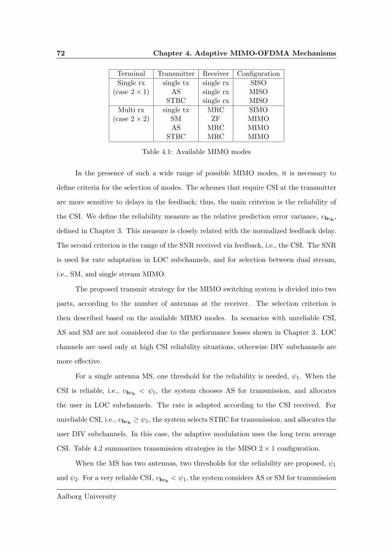
72 Chapter 4. Adaptive MIMO-OFDMA Mechanisms
Terminal Transmitter Receiver Configuration
Single rx single tx single rx SISO(case 2 × 1) AS single rx MISO
STBC single rx MISO
Multi rx single tx MRC SIMO(case 2 × 2) SM ZF MIMO
AS MRC MIMOSTBC MRC MIMO
Table 4.1: Available MIMO modes
In the presence of such a wide range of possible MIMO modes, it is necessary to
define criteria for the selection of modes. The schemes that require CSI at the transmitter
are more sensitive to delays in the feedback; thus, the main criterion is the reliability of
the CSI. We define the reliability measure as the relative prediction error variance, υhǫh ,
defined in Chapter 3. This measure is closely related with the normalized feedback delay.
The second criterion is the range of the SNR received via feedback, i.e., the CSI. The SNR
is used for rate adaptation in LOC subchannels, and for selection between dual stream,
i.e., SM, and single stream MIMO.
The proposed transmit strategy for the MIMO switching system is divided into two
parts, according to the number of antennas at the receiver. The selection criterion is
then described based on the available MIMO modes. In scenarios with unreliable CSI,
AS and SM are not considered due to the performance losses shown in Chapter 3. LOC
channels are used only at high CSI reliability situations, otherwise DIV subchannels are
more effective.
For a single antenna MS, one threshold for the reliability is needed, ψ1. When the
CSI is reliable, i.e., υhǫh < ψ1, the system chooses AS for transmission, and allocates
the user in LOC subchannels. The rate is adapted according to the CSI received. For
unreliable CSI, i.e., υhǫh ≥ ψ1, the system selects STBC for transmission, and allocates the
user DIV subchannels. In this case, the adaptive modulation uses the long term average
CSI. Table 4.2 summarizes transmission strategies in the MISO 2 × 1 configuration.
When the MS has two antennas, two thresholds for the reliability are proposed, ψ1
and ψ2. For a very reliable CSI, υhǫh < ψ1, the system considers AS or SM for transmission
Aalborg University

4.2 Transmit Strategy 73
Feedback MIMO mode Allocation CSI for AMC
Reliable CSI AS LOC subchannel predicted SNRυhǫh < ψ1
Unreliable CSI STBC DIV subchannel long term average SNRυhǫh ≥ ψ1
Table 4.2: Selection criterion for the transmit strategy in MISO 2 × 1
Feedback MIMO mode Allocation CSI for AMC
Reliable CSI AS-MRC or SM LOC subchannel predicted SNRυhǫh < ψ1
Reliable CSI AS-MRC LOC subchannel predicted SNRψ1 ≤ υhǫh < ψ2
Unreliable CSI STBC-MRC DIV subchannel long term average SNRυhǫh ≥ ψ2
Table 4.3: Selection criterion for the transmit strategy in MIMO 2 × 2
in LOC subchannels. The transmit mode that delivers the highest throughput is selected
on the basis of the predicted SNR. Typically, AS is better than SM at low SNR or in
strong spatial correlation scenarios. A mid-range interval of reliability, ψ1 ≤ υhǫh < ψ2,
is justified by the different sensitivity of dual and single stream modes to delay. In this
interval, AS is selected for transmission, and the MS is allocated in LOC subchannels.
The rate level is obtained based on the CSI received in the feedback message. When the
feedback is unreliable, i.e., υhǫh ≥ ψ2, the BS transmits over both antennas using STBC,
allocates DIV channels, and selects rate based on long term average SNR. Table 4.3
summarizes transmission strategies in the MIMO 2 × 2 configuration.
We consider two separate blocks for the adaptive MIMO and adaptive rate schemes
based on feedback, as represented in Figure 4.8. The BS selects the MIMO mode by
analysis of long term average SNR and normalized feedback delay. The rate selection
depends on the frame SNR estimation and on the updated SNR thresholds. Section 4.2.1
proposes the MIMO look-up tables with the values of the reliability thresholds found as a
result of the analysis of throughput achieved with each scheme.
The description of the switching process is also presented in the form of flowcharts
in Figures 4.9 and 4.10 to identify the actions described above for the cases of single or
multiple antennas at the receiver, respectively.
Daniel Vaz Pato Figueiredo

74 Chapter 4. Adaptive MIMO-OFDMA Mechanisms
Rate Selector
MIMO Selector
Long term average SNR
Measure Frame SNR
System normalized
delay
Figure 4.8: Flowchart of MIMO switching mechanism
AS
Reliability measure
STBCAS
Flowchart at MS
Measure SNR
STBC
SNR thresholds
Feedback CSI
Rate selection Rate selection
MIMO look-up
table
Flowchart at BS
Figure 4.9: Flowchart for downlink MISO 2 × 1 configuration
Aalborg University

4.2 Transmit Strategy 75
SM
Reliability measure
STBCSM
Flowchart at MS
Measure SNR
STBC+MRC
SNR thresholds
Feedback CSI
Rate selection Rate selection
MIMO look-up
table
Flowchart at BS
AS+MRC
Rate selection
AS
Figure 4.10: Flowchart for downlink MIMO 2 × 2 configuration
4.2.1 MIMO Look-up Tables
The proposed MIMO switching mechanism requires the a priori information on the inter-
vals of channel and feedback conditions that favor each MIMO mode. Look-up tables are
an efficient solution for feedback based adaptive techniques.
The MIMO mode selector checks from the look-up table the technique that delivers
the highest performance for each pair of delay-SNR. Hence, the MIMO look-up table fits
into a two-dimensional space, based on the channel quality and feedback delay. For a given
scenario, we tune the system for each combination of SNR and delay, i.e., the mechanism
selects the MIMO mode that delivers the highest spectral efficiency in a Rayleigh fading
channel.
The look-up table is static for a given scenario and is saved at the BS. The proposed
system measures the long term average SNR of the link and keeps track of the feedback
delay and time variability of the channel, and uses the SNR and delay thresholds to switch
MIMO scheme according to the look-up table.
Daniel Vaz Pato Figueiredo

76 Chapter 4. Adaptive MIMO-OFDMA Mechanisms
0
.03
.06
.09
.12
.15
0 10 20 30 40
Legend
AS
STBCN
orm
aliz
ed F
eedb
ack
Del
ay
SNR average
Figure 4.11: MISO 2 × 1 look-up table
Following the transmission strategy described above, two cases are considered: the
single antenna MS, and the dual antenna MS. We select best performing MIMO configura-
tion for a range of feedback delays. The MISO 2×1 look-up table, depicted in Figure 4.11,
is obtained by choosing the scheme with the highest throughput for each combination of
average SNR and delay. From the available single transmitter modes, only AS and STBC
are selected, since the SISO is outperformed in all conditions. AS is preferred for lower
delays, while STBC proves to be more robust for a high feedback delay.
Figure 4.12 shows the adaptation when there is no delay in the feedback. In this case,
the system chooses AS for transmission over the full range of SNR conditions. Thus, the
curve of the adaptive system overlaps the performance curve of AS. When a normalized
delay of 0.10 is experienced by the feedback channel, the system uses AS for transmission
at low SNR, and selects STBC at high SNR conditions, as shown in the look-up table.
Figure 4.13 depicts the performance of the adaptive system that overlaps the performance
with the highest throughput scheme at each SNR value.
Following the same procedure for the modes available with two receive antennas, we
obtain the MIMO 2 × 2 look-up table depicted in Figure 4.14. In this case, SM delivers
the highest throughput. However, it is more sensitive to the feedback delay; therefore,
it is preferred in low delay scenarios and good channel conditions. The more robust
STBC delivers higher performance at higher delays, while AS is preferred at poor channel
conditions and low to mid-range delay scenarios.
Aalborg University

4.2 Transmit Strategy 77
0 5 10 15 20 25 30 35 400
1
2
3
4
5
6
7
8
Average SNR (dB)
AS
STBC
AdaptS
pe
ctr
al e
ffic
ien
cy
Figure 4.12: Spectral efficiency of MISO 2 × 1 look-up table with no delay
0 5 10 15 20 25 30 35 400
1
2
3
4
5
6
7
8
Average SNR (dB)
AS
STBC
Adapt
Sp
ectr
al e
ffic
ien
cy
Figure 4.13: Spectral efficiency of MISO 2 × 1 look-up table with fdτ = 0.10
Daniel Vaz Pato Figueiredo

78 Chapter 4. Adaptive MIMO-OFDMA Mechanisms
0
.03
.06
.09
.12
.15
0 10 20 30 40
Legend
AS + MRC
SM
STBC + MRC
Nor
mal
ized
Fee
dbac
k D
elay
SNR average
Figure 4.14: MIMO 2 × 2 look-up table
0 5 10 15 20 25 30 35 400
2
4
6
8
10
12
14
16
Average SNR (dB)
SM
Adapt
AS-MRC
STBC-MRC
Sp
ectr
al e
ffic
ien
cy
Figure 4.15: Spectral efficiency of MIMO 2 × 2 look-up table with no delay
Figures 4.15 and 4.16 show the results for the cases with no feedback delay and with
a normalized delay of 0.09, respectively. In the case of no delay, the system selects AS at
low SNR of up to 20 dB and switches to SM at higher values of SNR. In the presence of a
normalized feedback delay lower than 0.09, the adaptation continues to switch between AS
and SM, but with a threshold observed at higher SNR as seen in Figure 4.16. For delays
higher than 0.1, STBC achieves higher throughput than SM in good channel conditions,
and it is the preferred choice for all the SNR range for delays higher than 0.15.
For a single receive antenna terminal, the MIMO selection switches between AS and
STBC, whereas for a multiple antenna terminal, the scheme includes the SM option, and
Aalborg University

4.2 Transmit Strategy 79
0 5 10 15 20 25 30 35 400
1
2
3
4
5
6
7
8
9
10
Average SNR (dB)
AS-MRC
STBC-MRC
SM
Adapt
Sp
ectr
al e
ffic
ien
cy
Figure 4.16: Spectral efficiency of MIMO 2 × 2 look-up table with fdτ = 0.09
more transition values are necessary.
The MIMO look-up table proves to be useful in a system that supports terminals
with various speeds. For a wide range of mobility, the BS deals with stationary, as well
as fast speed users. The MSs in the first category experience an almost constant channel,
while the high velocity MSs have a time-variant channel, therefore, a high normalized
feedback delay. In this heterogeneous scenario, the MIMO look-up table accommodates
all users according to their channel time variability, which would not be possible with a
fixed MIMO solution.
4.2.2 Summary
This section described the transmit strategies of a MIMO switching system combined with
rate adaptation. We have detailed the actions and flowcharts of the proposed scheme, and
the threshold values were presented in the form of a MIMO look-up table.
The system shows more advantages in scenarios with users at various levels of mo-
bility, since supporting stationary users involves substantially different approach than fast
speed MS.
Daniel Vaz Pato Figueiredo

80 Chapter 4. Adaptive MIMO-OFDMA Mechanisms
4.3 Feedback Design Issues
In the simulation results shown so far, the modulation level is selected on a symbol by
symbol basis, i.e., the MS measures and sends via feedback the SNR of every symbol.
In a more practical approach, as presented in the system description of Section 4.1, the
feedback reports the channel quality experienced in a frame received at the MS. On the
basis of the feedback received, the BS chooses the rate to apply in the next downlink
frame.
The analytical design of SNR thresholds updated with the feedback delay faces
two important issues in such frame based feedback. First, the optimal SNR value to be
reported in the feedback has to be defined. Second, the optimal length for the delay to be
considered has to be chosen. A comparison of different solutions for these issues is tackled
in Sections 4.3.1 and 4.3.2.
4.3.1 Reporting SNR of a Frame
In a mobility scenario, the SNR varies from symbol to symbol within the downlink frame.
On the basis of the SNR estimated for all symbols, the feedback reports one value of SNR
for the received frame. Although this parameter is bounded by the placement of the pilots
in the frame, we assume a perfect channel estimation for all symbols in the frame.
It is usual to report the average SNR across all symbols within the frame. However,
other solutions of using single symbols can also be advantageous. We consider the cases
of selecting the SNR of the first symbol in the frame, the average across all symbols of the
frame, and the last symbol in the frame. The last symbol has a higher time correlation
with the frame where the information will be used, i.e., the delay is lower, but it captures
only one symbol. Figure 4.17 depicts a representation of the three options to report the
SNR value.
Results were obtained for a normalized frame duration of 0.05 and a normalized
feedback delay of 0.1. These values occur for a scenario where a system with carrier
frequency of 2 GHz and frame duration of 1 ms supports users at the speed of 27 km/h,
Aalborg University

4.3 Feedback Design Issues 81
DL Frame 1 MS measures SNR
Duration
UL Frame Feedback Delay
DL Frame 2 BS transmits AMC level
Figure 4.17: Reporting the SNR of a frame
0 5 10 15 20 25 30 35 400
1
2
3
4
5
6
7
8
Average SNR (dB)
Avg Frame
First Symb Frame
Last Symb Frame
5 10 20 25 30 35
Sp
ectr
al e
ffic
ien
cy
Figure 4.18: Spectral efficiency for different reported SNR with fdτ = 0.1
and the feedback delay corresponds to two frames. Figure 4.18 presents the results for the
different options of selecting the CSI for feedback, based on the SNR of symbols of the
frame. On account of a higher time correlation between the measure and the adaptation
at the BS, reporting the SNR of the last symbol of the frame is shown to achieve the best
performance. This solution provides the CSI with the lowest gap between received frame
at MS and transmitted frame from the BS, and it reveals more gain at mid-range SNR.
4.3.2 Length of Delay between Frames
In the system proposed in this chapter, the BS receives the feedback from the terminal, and
then it chooses the modulation level based on the updated thresholds, computed with the
Daniel Vaz Pato Figueiredo

82 Chapter 4. Adaptive MIMO-OFDMA Mechanisms
DL Frame 1 MS measures SNR
Duration 1
Duration 2
Duration 3
UL Frame Feedback Delay
DL Frame 2 BS transmits AMC level
Figure 4.19: Different durations for designing AMC thresholds
knowledge of the feedback delay. The length of the delay between the symbol when the MS
measures the SNR and the downlink frame at BS may have various interpretations. The
duration of the delay can be calculated with respect to the first symbol, the middle, or the
last symbol of the transmitted frame at the BS. Following the results from Section 4.3.1,
the SNR of the last symbol of the received frame is reported via feedback. Figure 4.19
shows the different delays considered.
Figure 4.20 depicts the spectral effiency of the system when using updated SNR
thresholds computed with the different delays. As in the previous section, the frame
has a normalized length of 0.05, and a normalized feedback delay of 0.1. The Duration
1 corresponds to a normalized delay of 0.075 in the design of updated SNR thresholds,
whereas Duration 2 and Duration 3 represent values of 0.1 and 0.125 of normalized delay,
respectively.
The analysis of the results suggests that the three regions of average SNR should
be considered separately. At poor channel conditions, with an SNR below 15 dB, the
thresholds computed from the lowest delay, referred to as Duration 1, achieve better
performance. As the updated thresholds are conservative in the rate adaptation, a higher
delay considered implies a later start in the rise of the curve. In fact, considering a delay
of 0.075, the system needs 10 dB to deliver 0.5 Mbit/s/Hz, while in a scenario with 0.125
delay, the system achieves the same throughput only at 17 dB of average SNR. In the
range of 15 to 32 dB, the highest throughput is obtained with the normalized length 0.1.
This delay considers the middle point of the frame and is more accurate for the symbols
around the center of the frame when compared to the extremes, providing the highest
Aalborg University

4.3 Feedback Design Issues 83
0 5 10 20 25 30 35 400
1
2
3
4
5
6
7
8
Average SNR (dB)
Sim Upd Thr AMC delay .075
Sim Upd Thr AMC delay .1
Sim Upd Thr AMC delay .125
15
Sp
ectr
al e
ffic
ien
cy
Figure 4.20: Spectral efficiency of different AMC thresholds with fdτ = 0.1
accuracy coverage of the frame. Above 32 dB, the SNR thresholds based on the duration
with respect to the last symbol of the frame, Duration 3, deliver the highest performance.
The high delay allows for a conservative and assured selection of rate, a preferable choice
in very good SNR conditions.
On the basis of these findings, an adaptive approach to determine the best delay in
the computation of thresholds for each region can be used. However, this adaptation is
very sensitive to different scenarios. A more general approach consists of using the time
delay between the last symbol of the frame at MS and the middle of the frame at BS,
since it outperforms the other options in the mid-range SNR.
4.3.3 Summary
This section evaluated and proposed two features of the feedback design in the context of
rate selection on a per frame basis. The analysis suggests that the MS measures the SNR
of the last symbol of the received frame to send in feedback, and that the thresholds take
into account the delay with respect to the center of the downlink frame.
Daniel Vaz Pato Figueiredo

84 Chapter 4. Adaptive MIMO-OFDMA Mechanisms
4.4 Conclusions
This chapter proposed the general framework and specific mechanisms for a MIMO-
OFDMA system. The focus was the design of a system that is aware of error in adapting
to outdated channel information.
We proposed a MIMO switching mechanism based on the analysis of channel con-
ditions and a measure of the channel information reliability delivered by the feedback. In
accordance with this system, MIMO look-up tables were presented in a two-dimensional
perspective to indicate the most favorable MIMO mode in a grid of average SNR and
normalized feedback delay.
In terms of feedback design, the terminal should report to the BS the SNR of the
last symbol of the received frame. Furthermore, the SNR thresholds should be computed
based on a delay with respect to the center of the transmitted frame.
Having proposed a mechanism to select the MIMO mode on the basis of the perfor-
mance and channel statistics of the link-level, in the next chapter, we assume a system-level
perspective of cellular networks, and analyze the interference effects in MIMO and OFDM
systems.
Aalborg University

Chapter 5
Cochannel Interference and
Asynchronous OFDM
The previous chapters described various MIMO techniques, link adaptation, and feedback
issues at the link level. This chapter focuses on the system aspects of OFDM cellular
networks, CCI, and asynchronous interference. Due to a high demand for spectrum use,
CCI is one of the main sources of performance degradation in a cellular wireless system.
Although transmit spatial diversity has been proposed in various standards as an effective
mean to enhance wireless link reliability, the interaction of MIMO diversity techniques
with CCI is still an open topic of research [B06]. In addition, the presence of cochannel
signals in OFDM networks introduces additional interference that the system should cope
with.
Cellular radio systems suffer from CCI in the downlink that arises from neighbor
BSs transmissions. Such scenario is commonly encountered at the cell edge of urban
macrocells, and the assumption of Rayleigh fading for both the desired and interfering
signals is usually appropriate since both links experience deep fading from the terminal to
the base station. Spatial diversity is an effective tool to provide robustness in the link at cell
edge. Open-loop transmit diversity and receiver MRC are considered for the desired link.
The analysis of the average probability of bit error of M-ary QAM considers the presence
85

86 Chapter 5. Cochannel Interference and Asynchronous OFDM
of multiple independent interferers. The results are applicable to systems employing open-
loop transmit diversity and MRC with coherent demodulation. The study analyzes the
interaction between the number of equal power interferers and the spatial diversity order.
Asynchronous signals in OFDM system introduce additional interference in the per-
formance of both broadcast and unicast scenarios. Even with synchronized transmissions
at all BSs in the cellular scenario, the delay between cochannel signals arriving at the ter-
minal increases the interference level creating ISI into the OFDM system [And05]. A larger
cell radius of a hexagonal cellular layout increases the delays of the signals from neigh-
bor BSs. In the unicast scenario, we consider linear receivers for interference cancelation,
MRC and MMSE, to cope with CCI signals arriving from different BSs. Furthermore, we
compare the performance of a suboptimal receiver based on the received signal covariance
matrix.
The chapter is outlined as follows. Section 5.1 investigates the performance of spa-
tial diversity systems in a scenario limited by CCI. Section 5.2 focuses on the effect of
asynchronous received signals in the downlink of OFDM cellular scenarios for broadcast
and unicast transmissions using spatial diversity. Section 5.3 concludes the chapter.
5.1 Effect of Cochannel Interference on Spatial Diversity
This section investigates the average probability of bit error performance of spatial diver-
sity in the presence of independent equal power interferers. The performance of receive
diversity in a fading environment with AWGN and CCI is traditionally measured in terms
of outage probability, i.e., the probability of a user to be deprived of the service. Never-
theless, the average BER is also used to describe the performance of such systems as an
important measure to determine the robustness of the link [CS99]. The average bit error
rate in an MRC system that has independent interferers with identical or distinct mean
powers was derived in [CA03]. In addition, the authors in [BZR05] present a compari-
son, in terms of statistical gain differences, of optimal combining and MRC algorithms
in presence of interference. The interaction between the number of interferers and the
Aalborg University

5.1 Effect of Cochannel Interference on Spatial Diversity 87
OFDM Modulator
MIMO encoder
Channel estimation
MIMO decoder H OFDM
Demod
g 2
g 1 Interf 1
Interf 2
Figure 5.1: System model of MIMO desired link with multiple single antenna cochannelinterferers
spatial diversity order studied here helps to understand the impact of using multiantennas
in interference limited scenarios.
5.1.1 System Model
This section considers the downlink MIMO diversity channel, where both the BS and
terminal have multiple antennas to exploit diversity. Moreover, we consider a number
of single antenna interfering signals present at all diversity branches, as represented in
Figure 5.1.
At the receiver end, the signals at the Nr antennas are weighted using MRC to
maximize the output SNR. Although it is known that MRC is suboptimal in the presence
of non-spectrally white interference, it is a practical blind technique for most communica-
tion standards that include MIMO diversity. The channel estimation of the desired link
is assumed perfect at the receiver. The Nt antennas at the transmitter encode the signal
using an orthogonal open-loop transmit diversity scheme, STBC.
Considering L interferers with one transmit antenna each, the interference channel
fading model may be written as
y =
√Es
NtHs +
L∑
i=1
√Eigisi + w ,
Daniel Vaz Pato Figueiredo

88 Chapter 5. Cochannel Interference and Asynchronous OFDM
where H[Nr×Nt] is the channel matrix, y is the signal at the receiver array, s is the desired
transmitted signal, si is the interferer i transmitted signal, and gi is the channel of the
single-antenna interferer i. Here, Es and Ei are the powers of the desired and interfering
users, respectively, while w is the complex AWGN with zero mean and variance N0.
When employing orthogonal open-loop transmit diversity, and MRC at the receiver
using the knowledge of the desired signal channel, the detected signal is calculated from
HHy =
√Es
NtHHHs +
L∑
i=1
√EiH
Hgisi + HHw ,
where (.)H denotes the Hermitian transpose. In this case, the Signal to Interference and
Noise Ratio (SINR), γ, can be written as
γ =1
Nt‖H‖2
FEs
N0∑Li=1
|HHgi|2‖H‖2
F
Ei
N0+ 1
, (5.1)
where Es
N0and Ei
N0are the average pre-processing SNR of desired link and Interference to
Noise Ratio (INR) of user i. We define ρa = Es
N0as the average pre-processing SNR per
spatial link, and ρI = Es
N0as the average pre-processing INR contribution of each interferer
at the receive antenna. ‖H‖2F ≡ tr(HHH) =
∑Nr
p=1
∑Nt
q=1 |hp,q|2 is the squared Frobenius
norm, i.e., the total power gain of the channel. We use (5.1) in the following section to
characterize statistically the detected SINR.
5.1.2 Channel Statistics for Diversity and Interference
The wireless channel is a flat fading channel varying in time according to the classical
Doppler. We assume the channel to be slowly time-varying, so that it is approximately
constant for two consecutive symbols. The multipath fading environment is characterized
by the Rayleigh fading channel for both the desired and interfering links. This scenario
can be found in cellular radio systems, where neighbor cells introduce CCI in the desired
link. Moreover, all the diversity branches of the desired link and the interfering signals
are assumed to fade independently.
Aalborg University

5.1 Effect of Cochannel Interference on Spatial Diversity 89
Under these assumptions, the SNR of the desired signal follows a chi-square dis-
tribution with 2NtNr degrees of freedom, as presented in Appendix D.3, and its PDF is
given by
A =1
Nt‖H‖2
Fρa ,
fA(a) =aNtNr−1
Γ(NtNr)(
ρa
Nt
)NtNrexp
(− a
ρa
Nt
).
Considering L equal power interferers, the total INR was proved in [CS99] to follow
a chi-square distribution with 2L degrees of freedom:
B =L∑
i=1
|HHgi|2‖H‖2
F
ρI ,
fB(b) =bL−1
Γ(L) (ρI)Lexp
(− b
ρI
).
By taking the interpretation of the SINR as SINR = SNRINR+1 , i.e., γ = A
B+1 , its
PDF can be obtained from the distributions of SNR and INR employing the integration
property for independent variables,
fγ(γ) =
∫ ∞
0(w + 1)fA ((w + 1)γ) fB(w) dw . (5.2)
Using the distributions of the random variables described above, it has been proved
in [CA03, AR01] that the density function of the SINR is derived with the modified
canonical distribution, thus obtaining a closed-form:
fγ(γ) =γNtNr−1
Γ(NtNr)Γ(L)(
ρa
Nt
)NtNrexp
(−γNt
ρa
)NtNr∑
n=0
CNtNrn
(ρI)nΓ(L+ n)(
ρINt
ρa γ + 1)L+n
. (5.3)
The expression of the distribution of the SINR (5.3) is used below to derive the
average probability of bit error.
Daniel Vaz Pato Figueiredo

90 Chapter 5. Cochannel Interference and Asynchronous OFDM
5.1.3 Average Probability of Bit Error
This section presents the analytical study of the average probability of bit error. The
mean BER, Pb, is obtained by averaging over the PDF of the SINR given in (5.3),
Pb(M) =
∫ ∞
0Pb(M,γ)fγ(γ)dγ , (5.4)
where M is the order of the modulation employed, and Pb(M,γ) is the BER in AWGN.
Several approaches can be followed in order to obtain a closed-form approximation of (5.4),
and to study the performance of each technique with respect to the average probability of
bit error.
As shown in Appendix E.1, the approximation for the probability of bit error valid
for M-QAM is
Pb(M,γ) ≈ 0.2 exp
(−γ 1.6
M − 1
). (5.5)
Note that the approximation of this formula is tight for lower order modulations; thus, in
order to ensure an accuracy of up to 1 dB, we target modulations lower than or equal to
64-QAM.
By applying (5.5) and (5.3) to (5.4), we derive the average probability of error:
Pb(M) ≈ 0.2
Γ(NtNr)(
ρa
Nt
)NtNr
NtNr∑
n=0
CNtNrn (ρI)n Γ(L+ n)
Γ(L)
×∫ ∞
0
γNtNr−(L+n+1)
(1γ + NtρI
ρa
)L+nexp
[−γ(Nt
ρa+
1.6
M − 1
)]dγ ,
where the integral in this expression still has no known closed-form expression. However,
in a high Signal to Interference Ratio (SIR) scenario, e.g., when the user is close to the cell
center with a strong desired signal, but some interference from neighbor BSs still exists,
Aalborg University

5.1 Effect of Cochannel Interference on Spatial Diversity 91
the expression can be simplified, using a hign-SNR approximation ρI
ρa → 0, to
Pb(M) ≈ 0.2
Γ(NtNr)(
ρa
Nt
)NtNr
NtNr∑
n=0
CNtNrn (ρI)n Γ(L+ n)
Γ(L)
×∫ ∞
0γNtNr−1 exp
[−γ(Nt
ρa+
1.6
M − 1
)]dγ .
The average BER can then be approximated in closed-form as
Pb(M)|SIR≫1 ≈ 0.2(1 + 1.6
M−1ρa
Nt
)NtNr
NtNr∑
n=0
CNtNrn (ρI)n Γ(L+ n)
Γ(L). (5.6)
The next section argues that a closed-form expression of the average bit error prob-
ability allows a better understanding of the interactions between spatial diversity and
interference.
5.1.4 Results and Discussion
This section presents analytical results of a system with multiple equal power interferers
in a Rayleigh fading scenario, and with QPSK transmission.
As mentioned in the previous section, the exact closed-form for the average BER
(5.4) is unknown; thus, this expression can be approximated with a numerical integration
method. Using a trapezoidal numerical integration, we evaluate the performance of a
MIMO diversity system in the presence of interferers. Figure 5.2 depicts the mean BER,
Pb(M), versus the number of interferers for a system employing QPSK modulation and
coherent detection. The result is based on the standard formula for Pb under AWGN that
is shown in Appendix B in (B.1). The analysis assumes that all the interferers have the
same power-to-noise ratio, ρI = 0 dB, and the number of interferers present in the system
varies. Figure 5.2 represents the degradation of a MIMO diversity system when increasing
the number of interferers, i.e., raising the total interference power.
It is worthwhile noting that the performance gain obtained with transmit antennas
disappears faster than the gain obtained with receive antennas, see Figure 5.2. Even in
Daniel Vaz Pato Figueiredo

92 Chapter 5. Cochannel Interference and Asynchronous OFDM
0 5 10 15 20 25 30 35 4010
−6
10−5
10−4
10−3
10−2
10−1
100
Average Bit Error Rate for QPSK
Number of Interferers (L)
Pb
Nt=1,N
r=1
Nt=2,N
r=1
Nt=1,N
r=2
Nt=2,N
r=2
Figure 5.2: Average BER versus the number of interferers with high power. SNR ρa =20 dB, and INR per interferer ρI = 0 dB
a high interference scenario, there is a gain when using MRC compared to SISO, while a
higher number of transmit antennas does not improve the performance significantly. For
instance, at a BER of 10−2, receive diversity can cope with up to thirteen interferers, while
transmit diversity can cope with only five interferers. This effect can be explained by the
presence of array gain in MRC scheme that makes the scheme more robust to interference,
compared to open loop transmit diversity.
In Section 5.1.3, we propose a closed-form expression (5.6) for the asymptotic analy-
sis of the average probability of bit error. In order to assess the accuracy of this expression,
we consider a scenario with a desired signal SNR of 20 dB and multiple interferers, each
having an INR of −10 dB, thus satisfying high SIR condition. Figure 5.3 illustrates the
average BER for both methods of approximation, i.e., the numerical integration and the
asymptotic closed-form. As the SIR increases, the curves tend to overlap, then validating
the approach in the asymptotic analysis.
An important factor in the analysis of the interference in MIMO diversity systems
is the effect of the number of interference sources to the average probability of bit error.
Therefore, we consider a constant total interference power, ρItotal, and vary the number of
Aalborg University

5.1 Effect of Cochannel Interference on Spatial Diversity 93
0 5 10 15 2010
−7
10−6
10−5
10−4
10−3
10−2
10−1
Average Bit Error Rate for QPSK
Number of Interferers (L)
Pb
Nt=1,N
r=1
Nt=2,N
r=1
Nt=1,N
r=2
Nt=2,N
r=2
Figure 5.3: Average BER versus the number of interferers with low power. SNR isρa = 20 dB and INR per interferer is ρI = −10 dB. The lines with ’◦’ represent theapproximation of the closed form expression (5.6)
interferers. Moreover, we consider that each interferer has the same power, i.e., the total
interference power is shared among the interferers with INR of ρI =ρI
total
L . Figure 5.4 shows
the closed-form expression of Pb(M) versus the number of interferers for different MIMO
configurations. Assuming the same total interference power, we see that the performance
of a SISO link is independent of the number of active interferers in the system. However,
when spatial diversity is higher than one, the impact of the number of interferers appears.
In fact, when exploiting diversity at mid SINR range, the average BER turns out to be
lower with a larger number of weak interferers than with fewer strong interference sources.
In order to understand the relation between the number of interferers and the
spatial diversity, we analyze the closed-form expression in the asymptotic behavior of
Pb(M)|SIR≫1. From (5.6), we can separate the sum in n and use the property of the
Daniel Vaz Pato Figueiredo

94 Chapter 5. Cochannel Interference and Asynchronous OFDM
1 2 3 4 5 6 7 810
−5
10−4
10−3
10−2
10−1
Average Bit Error Rate for QPSK
Number of Interferers (L)
Pb
Nt=1,N
r=1
Nt=2,N
r=1
Nt=1,N
r=2
Nt=2,N
r=2
Figure 5.4: Average bit error rate versus the number of interferers when the SINR remainsconstant. SNR is ρa = 25 dB and total INR is LρI = 10 dB, i.e., a constant SINR ofγ ≈ 14.6 dB
complete gamma function, Γ(a) = (a− 1)!, to obtain the following expression:
Pb(M)|SIR≫1 ≈ 0.2(1 + 1.6
M−1ρa
Nt
)NtNr
×[1 +NtNrρ
Itotal +
NtNr∑
n=2
CNtNrn (ρI
total)n
n−1∏
k=1
(1 +
k
L
)]. (5.7)
Note that for NtNr = 1, the value of Pb(M)|SIR≫1 does not depend on the number of
active interferers L, but it only depends on the total power of interference. Moreover, as
observed in numerical evaluation, when the spatial diversity of the desired signal increases,
i.e., NtNr ≥ 2, the number of equal power interferers affects the average probability of bit
error. In fact, for a given diversity order, a lower value of L will increase the probability of
bit error. The last product term of (5.7) also shows that a higher diversity order system
is more sensitive to the value of L. However, this effect is only valid for low number of
interferers. Figure 5.4 shows that Pb tends to be constant for L > 6.
Aalborg University

5.2 Asynchronous Cochannel Signals in Cellular OFDM Systems 95
5.1.5 Summary
In this section, we studied the impact of CCI on the performance of a spatial diversity
link. The average probability of bit error is evaluated considering that both the interfering
and desired signals experience Rayleigh fading channels. Transmit diversity proved to be
less robust to an increase in the number of interferers, compared to receive diversity. We
derived a closed-form expression for the asymptotic performance of average probability of
bit error, and used it to explain the relation between the number of interferers and the
diversity order of the system.
In the case of a constant total interference power, the number of active interferers
was shown to have impact on the performance of a system with spatial diversity. More
specifically, we showed that it is preferable to have multiple weak interferers when com-
pared to one single strong interferer, and this effect tends to be more marked with the
increase of the diversity order at mid-range SINR conditions.
5.2 Asynchronous Cochannel Signals in Cellular OFDM Sys-
tems
This section focuses on the impact of time-delayed signals in OFDM cellular scenarios. Due
to its relevance in intercell interference, two configurations are considered for transmission
in the downlink, broadcast and unicast.
In the OFDM downlink of both unicast and broadcast schemes, the asynchronous
signals at the terminal, originated at different BSs, create an additional source of inter-
ference, i.e., ISI. This issue has a greater effect in the uplink, due to the asynchronism
among users [THJ05, And05]. However, in the downlink problem, even with synchronized
BSs, the differences in propagation delay create interference that is difficult to avoid with
simple receivers at the terminal side. Several algorithms have been proposed for downlink
intercell time synchronization at the receiver [KMAH02, JSC+07], and it is generally ac-
cepted that synchronized transmission from BSs is a practical assumption [And05, SH03].
Daniel Vaz Pato Figueiredo

96 Chapter 5. Cochannel Interference and Asynchronous OFDM
This section assumes a downlink channel with synchronized BSs and linear receivers at
the MS.
In broadcast transmission, the users at cell edge benefit from diversity gain by
combining the signals from different BSs, leading to increased performance. Nevertheless,
the long delays experienced by the terminal in the channel impulse response affect the
performance, and new channel models need to be defined [Col07].
In single-frequency cellular networks, the unicast transmission to the users at cell
edge experiences high levels of CCI. Although adaptive antenna arrays can be used to
minimize the CCI in single-frequency networks [LS99], this technique requires the channel
matrix coefficients to be available at the transmitter. Therefore, the effect of asynchronous
signals in the OFDM performance, as well as the robustness of MIMO diversity techniques
against CCI, still remains open to research [B06].
5.2.1 System Model
We consider the downlink of an OFDM system with L cochannel signals, as represented
in Figure 5.1 in Section 5.1. Additionally, this section focuses on system level aspects,
including a realistic number of interferers, and assuming that the received signals experi-
ence different propagation delays and pathloss from the BSs to the terminal. The OFDM
system uses a bandwidth of 10 MHz with 1024 subcarriers, and a CP length of 72 samples
that correspond to 4.67 µs, equivalent to the 3GPP LTE specifications [3GP06a]. The 600
available data subcarriers are allocated to one user. The implementation of the system in
the link-level simulator is described in Appendix G. Furthermore, two transmission types
are considered for the simulation of cochannel signals, broadcast and unicast.
5.2.1.1 Linear model for Unicast and Broadcast
A narrowband linear model describes the received signal at one OFDM subcarrier, and it
is used to decode the signal.
Aalborg University

5.2 Asynchronous Cochannel Signals in Cellular OFDM Systems 97
Broadcast All the BSs transmit the same data, while the receiver is considered to
perfectly estimate the combined channel. The narrowband linear model can be written as
y =
(√EsH +
L∑
i=1
√EiGi
)s + w + δ ,
where Es and H are the power and the channel matrix of the strongest signal, respectively.
The symbol s represents the data source transmitted in broadcast, Gi is the channel matrix
of the signal i, and Ei represents its power. Here, w is the AWGN, and δ corresponds
to the error introduced by the asynchronous nature of the other received signals in the
OFDM demodulation process.
Unicast The desired BS transmits the data at the same time as the interferers send
independent streams of information, i.e., CCI. When MRC receiver is considered, we
assume ideal channel knowledge of the desired link, and no information about interferers.
On the other hand, for the MMSE receiver, the system employs channel knowledge of the
desired and interfering links. The narrowband linear model is written as
y =√EsHs +
L∑
i=1
√EiGisi + w + δ ,
where si are the independently generated interfering data streams. As in the broadcast
case, Es and H are the power and the channel matrix of the desired signal, while Ei and
Gi are the power and the channel matrix of the interfering signal i, respectively.
5.2.1.2 Cellular Scenario
The scenario layout is represented in Figure 5.5, and it consists of a hexagonal grid cellular
scenario of two tiers with nineteen BSs and three sectors each, similar to the 3GPP eval-
uation method [3GP06a]. The letters in the figure identify the positions of the terminal
in the cell. Four positions correspond to the cell-edge users, A, B, C, and F. In addition,
two locations are considered in the mid-range of the cell, D and E.
Daniel Vaz Pato Figueiredo

98 Chapter 5. Cochannel Interference and Asynchronous OFDM
−4000 −3000 −2000 −1000 0 1000 2000 3000 4000−4000
−3000
−2000
−1000
0
1000
2000
3000
4000
A
BC
DE F
→→→
Cellular Scenario Layout
distance (m)
dist
ance
(m
)
Figure 5.5: Cellular scenario for a cell radius of 1000 m
As specified by [3GP07], the antenna pattern of a three sector BS has the directional
gain given by
A(θ) = −min
[12
(θ
θ−3dB
)2
, Am
], (5.8)
where −180◦ ≤ θ ≤ 180◦ is the angle between the direction of departure and the boresight
of the antenna, θ−3dB = 70◦ is the 3 dB beamwidth, and Am = 20 dBi. The boresight
points at the middle of the hexagonal cell side, as shown by the arrows in Figure 5.5,
and the antenna gain at the BS is 14 dBi. The serving BS, i.e., the closest BS to the
terminal, may have either one single transmit antenna in SIMO configuration, or two
spatially uncorrelated transmit antennas in MIMO configuration for the desired link. The
other BSs are assumed to have a single transmit antenna.
5.2.1.3 Channel Power Delay Profile
The multipath channel model used in this work is the Vehicular A model with 6 taps
[3GP07]. The average power and delay of the paths is depicted in Figure 5.6(a). We
assume that the links from all BSs to the terminal follow the same PDP.
In the cellular scenario described above, the user assigned to the central BS receives
Aalborg University

5.2 Asynchronous Cochannel Signals in Cellular OFDM Systems 99
0 1 2 3 4 5 6−8
−6
−4
−2
0
2
4Path Delay Profile, Channel TU06
delay (us)
Rel
ativ
e P
ath
Pow
er (
dB)
(a) power delay profile of TU 6 paths channel
0 2 4 6 8 10 12−30
−25
−20
−15
−10
−5
0
5
delay (us)
Rel
ativ
e P
ath
Pow
er (
dB)
Path Delay Profile of Cellular Scenario, Channel TU06, Position: C
BS 1BS 4BS 3BS 5BS 2BS 6BS 11BS 12BS 10
(b) power delay profile of the received signal
Figure 5.6: Average power of the channel paths of a terminal in position C of the cellularlayout with cell radius 1000 m
the signal from all BSs with a certain attenuation and delay that depends on its position
in the cell. The pathloss model considered is the macrocell scenario specified in [3GP07].
We assume that all the BSs are synchronized at transmission in the downlink, and focus
on the propagation time delay between the signal received from its own BS, and the signal
received from neighboring BSs. The channel PDP takes into account the delay between
that signal, in addition to the attenuation due to pathloss and antenna patterns. The
PDP experienced by a terminal in the position C of the cell is depicted in Figure 5.6(b).
The eight strongest neighboring BSs are considered for simulation of interference.
5.2.2 Effect of Cochannel Signals in Broadcast
The results for broadcast are obtained with a SIMO configuration between the closest BS
and the terminal, i.e., the BS has one transmit antenna, and the receiver has two antennas.
The system uses a 16-QAM modulation and 2/3 rate turbo code. The signals received are
properly weighted using MRC to maximize the output SNR.
In order to assess the effect of the delay between cochannel transmissions, we consider
the effect of two broadcast signals that arrive at the terminal separated by a certain time
delay. Although a stronger cochannel signal boosts the performance by providing diversity
for the link, when this delay is larger than the CP, it causes interference. In the OFDM
Daniel Vaz Pato Figueiredo

100 Chapter 5. Cochannel Interference and Asynchronous OFDM
8 8.5 9 9.5 10 10.5 11 11.5−8.5
−8
−7.5
−7
−6.5
−6
−5.5
Broadcast − SNRown
=8dB − SIMO x SISON
oise
Pow
er (
dB)
SNRtot
(dB)
T=0usT=4usT=6usT=8usT=10us
(a) noise and interference to desired signal powerratios
8 8.5 9 9.5 10 10.5 11 11.5
0.8
1
1.2
1.4
1.6
1.8
2
2.2
2.4
2.6
Broadcast − SNRown
=8dB − SIMO x SISO
Spe
ctra
l Effi
cien
cy (
b/s/
Hz)
SNRtot
(dB)
T=0usT=4usT=6usT=8usT=10us
(b) spectral efficiency
Figure 5.7: Effect of single interferer delays in broadcast
system, additional interference arises when the delay is such that part of the channel taps
arrive outside the CP. For this simulation, the power of the first signal is fixed to an SNR
of 8 dB, while one delayed cochannel signal is considered with increasing power, i.e., the
total SNR increases. The graph in Figure 5.7(a) shows, for various delays of the cochannel
signal, the noise power arising from the combined effect of white gaussian noise and ISI
due to channel taps arriving after the CP based on the combined PDP. The abscissa
of the graph shows the total SNR of the combined signals. At higher SNR, i.e., with
stronger cochannel signal arriving at a certain delay, the noise and ISI power increases.
As expected, this effect is only significant when the delay is greater than the length CP,
which is 4.67 µs.
Figure 5.7(b) shows the spectral efficiency at different delays. It is worthwhile noting
that when a long delay is experienced, there is a peak of performance in the balance of
powers of the first signal to arrive, and of the delayed cochannel signal. The stronger power
of the delayed signal degrades the performance, since it introduces ISI into the system.
The diversity benefit of broadcast is achieved only for delays up to 6 µs.
After studying the effect of a single delayed cochannel signal, we analyze the impact
of cellular configurations in broadcast transmissions. In the cellular scenario described
in Section 5.2.1.2, we analyze the performance of a terminal positioned at the cell edge,
Aalborg University

5.2 Asynchronous Cochannel Signals in Cellular OFDM Systems 101
−10 −5 0 5 100
0.1
0.2
0.3
0.4
0.5
0.6
0.7
0.8
0.9Broadcast Cellular Scenario − SIMO x SISO
Spe
ctra
l Effi
cien
cy (
b/s/
Hz)
SNR (dB)
0m1000m2000m3000m
Figure 5.8: Spectral efficiency of downlink cellular broadcast system for different cellradius. The modulation employed is QPSK and the coding rate is 1/2
position B. For simulation purposes, we consider the eight strongest signals arriving from
the neighboring BSs. In order to study the effect of the asynchronous signals on the OFDM
demodulation, we consider different radiuses for the cellular layout. A radius of 1000 m
corresponds to an Inter-Site Distance (ISD) of 1732 m. As the distance in-between the
BSs increases, the delay in-between the received signals at the terminal increases due to
larger propagation time differences. Therefore, a higher ISD of the scenario implies an
inherently looser time synchronization of the received signals. When strong signals arrive
out of the cyclic prefix duration, the OFDM symbol suffers ISI. In the following results,
the curve with legend “0 m” corresponds to a reference case, when both signals arrive at
the same time instant, i.e., no time delay.
The graph in Figure 5.8 depicts the spectral efficiency of the system with QPSK
modulation and 1/2 code rate in the position B in the cell. Only a slight degradation in
the throughput can be observed. The effect of asynchronous signals at the receiver can
be shown more clearly at higher modulation orders, since these are more sensitive. The
spectral efficiency of a user at cell edge employing 16-QAM with 2/3 coding rate is given
in Figure 5.9 for the same three cell radius. The results evidence a spectral efficiency loss
Daniel Vaz Pato Figueiredo
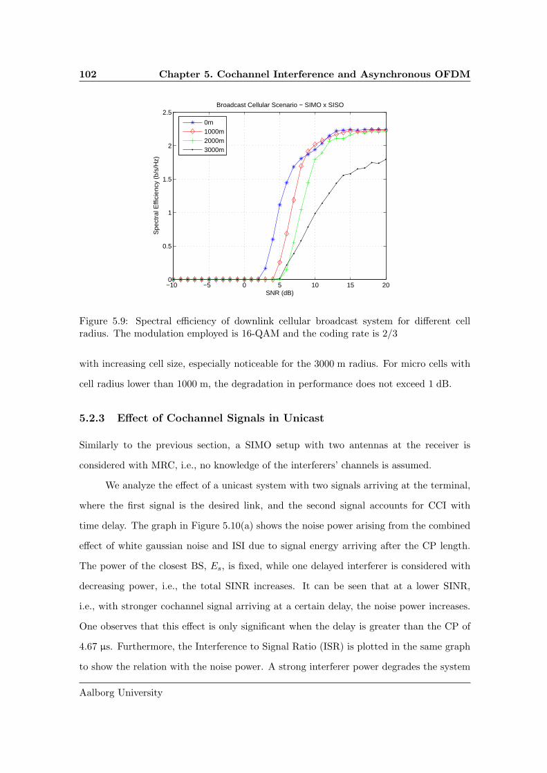
102 Chapter 5. Cochannel Interference and Asynchronous OFDM
−10 −5 0 5 10 15 200
0.5
1
1.5
2
2.5Broadcast Cellular Scenario − SIMO x SISO
Spe
ctra
l Effi
cien
cy (
b/s/
Hz)
SNR (dB)
0m1000m2000m3000m
Figure 5.9: Spectral efficiency of downlink cellular broadcast system for different cellradius. The modulation employed is 16-QAM and the coding rate is 2/3
with increasing cell size, especially noticeable for the 3000 m radius. For micro cells with
cell radius lower than 1000 m, the degradation in performance does not exceed 1 dB.
5.2.3 Effect of Cochannel Signals in Unicast
Similarly to the previous section, a SIMO setup with two antennas at the receiver is
considered with MRC, i.e., no knowledge of the interferers’ channels is assumed.
We analyze the effect of a unicast system with two signals arriving at the terminal,
where the first signal is the desired link, and the second signal accounts for CCI with
time delay. The graph in Figure 5.10(a) shows the noise power arising from the combined
effect of white gaussian noise and ISI due to signal energy arriving after the CP length.
The power of the closest BS, Es, is fixed, while one delayed interferer is considered with
decreasing power, i.e., the total SINR increases. It can be seen that at a lower SINR,
i.e., with stronger cochannel signal arriving at a certain delay, the noise power increases.
One observes that this effect is only significant when the delay is greater than the CP of
4.67 µs. Furthermore, the Interference to Signal Ratio (ISR) is plotted in the same graph
to show the relation with the noise power. A strong interferer power degrades the system
Aalborg University

5.2 Asynchronous Cochannel Signals in Cellular OFDM Systems 103
−2 0 2 4 6 8 10−20
−18
−16
−14
−12
−10
−8
−6
−4
−2
0Single Cochannel Interferer − SNR=10 dB − SIMO x SISO
Inte
rfer
ence
/Noi
se P
ower
(dB
)
SINR (dB)
T=0usT=4usT=6usT=10usISR
(a) noise and interference to desired signal powerratios
−2 0 2 4 6 8 100
0.5
1
1.5
2
2.5Single Cochannel Interferer − SNR=10 dB − SIMO x SISO
Spe
ctra
l Effi
cien
cy (
b/s/
Hz)
SINR (dB)
T=0usT=6usT=10us
(b) spectral efficiency
Figure 5.10: Effect of single interferer delays in unicast
performance proportionally to the ISR. For low SINR, the ISR effect is greater than the
interference due to the delay between signals, thus making the effects of interference and
time delay difficult to separate.
For the same simulation configuration, Figure 5.10(b) illustrates the spectral effi-
ciency at different delays. All the curves include the interference signal with power defined
by ISR, shown in previous graph. The performance degradation due to asynchronous inter-
ference is not as noticeable as in the broadcast case, since in this situation the performance
is limited by the interference power directly. Moreover, we note that the spectral efficiency
is also lower than in broadcast case.
After studying the effect of a single delayed cochannel interferer, we analyze the
impact of unicast transmissions in cellular configurations. Using the cellular scenario
described in Section 5.2.1.2, the simulations are run for a terminal situated in different
positions at the cell in a unicast system. The hexagonal cells have a radius of 1000 m, i.e.,
ISD of 1732 m. The receiver has two antennas, and the signals are combined using MRC,
assuming perfect channel estimation of the link with the serving BS. The channel gains of
the interfering BSs are unknown at the receiver. The spectral efficiency versus the desired
signal SNR is given in Figure 5.11.
Figure 5.12 depicts the performance of a terminal at the cell edge for various cell
Daniel Vaz Pato Figueiredo

104 Chapter 5. Cochannel Interference and Asynchronous OFDM
−10 −5 0 5 10 15 200
0.1
0.2
0.3
0.4
0.5
0.6
0.7
0.8
0.9
Spe
ctra
l Effi
cien
cy (
b/s/
Hz)
SNR (dB)
Cochannel Interference − Cellular Scenario − SIMO x SISO
ABCDEF
Figure 5.11: Spectral efficiency for different positions in the cell. Unicast signal withQPSK and MRC receiver
radiuses. A higher order of modulation is used in this simulation, since it is more sensitive
to the interference arising due to signal delays. Although with large cells the OFDM system
suffers degradation from the increased delays of asynchronous signals, the interference
power plays a more important role than the ISI effects. This can be seen by the ISR level
in Figure 5.10(b) and the moderate effect of delays in Figure 5.12.
5.2.4 Known Interference with MMSE Detection
MRC is a suboptimal approach for multiple antennas in the presence of cochannel inter-
ferers [CFS97]. Optimal combining is achieved at the cost of estimating the channel of
all interferers [SH98]. Figure 5.13 shows that the performance is increased when MMSE
receiver is used with the knowledge of the interfering channels. Higher gains in spectral
efficiency are obtained at cell edge, i.e., positions B, C, and F, where interference is high.
In the following, we study an MMSE-like receiver that does not require the knowledge of
the interfering signal channels.
This section investigates the gain in performance available by using interfering chan-
nel information at the receiver. In the presence of CCI, the optimal combining is achieved
Aalborg University

5.2 Asynchronous Cochannel Signals in Cellular OFDM Systems 105
0 5 10 15 20 25 300
0.2
0.4
0.6
0.8
1
1.2
1.4Cochannel Interference − Cellular Scenario − SIMO x SISO
Spe
ctra
l Effi
cien
cy (
b/s/
Hz)
SNR (dB)
0m1000m2000m3000m
Figure 5.12: Spectral efficiency for different positions in the cell. Unicast signal and16-QAM
−10 −5 0 5 10 15 200
0.1
0.2
0.3
0.4
0.5
0.6
0.7
0.8
0.9
Spe
ctra
l Effi
cien
cy (
b/s/
Hz)
SNR (dB)
Cochannel Interference − Cellular Scenario − SIMO x SISO
ABCDEF
Figure 5.13: Spectral efficiency for different positions in the cell. Unicast signal withQPSK and MMSE receiver
Daniel Vaz Pato Figueiredo

106 Chapter 5. Cochannel Interference and Asynchronous OFDM
using an MMSE receiver with the knowledge of the interfering link channels. We consider
a more practical case where the channel information is estimated from the received signal
without knowledge of the individual interferer channels. This is achieved by using an
estimate of the covariance matrix of the received signal as follows:
Ryy = E[yyH ] ,
y = yR−1yy .
In order to obtain a robust estimate of the covariance matrix, a large number of symbols is
needed for statistics. In a slow variation channel, the required period of analysis increases,
since we need to observe the channel for a longer period to obtain a closer estimate of the
real average.
The OFDM system has a Fast Fourier Transform (FFT) size of 1024 for a bandwidth
of 10 MHz, and we consider the speed of 3 km/h. At this speed, the coherence time of
the channel is 32.2 ms. Similarly, based on the RMS delay spread of the Vehicular A
channel profile, i.e., 370 ns [ITU97], the 50% coherence bandwidth is 430 kHz. We use an
averaging window to obtain an estimate of the covariance matrix of the received signal.
The window has 80 symbols, corresponding to 5.3 ms, and 6 subcarriers, corresponding to
58.6 kHz, i.e., it is within the coherence time and coherence bandwidth, respectively. The
averaging window choice is based on preliminary studies to maximize performance for the
time and frequency selectivity. We refer this scheme as Windowing-MMSE.
In a SIMO configuration of the desired channel, the performance at the cell edge
of a cellular scenario with ISD of 1732 m is shown in Figure 5.14. The performance of
MMSE with full channel knowledge is clearly superior to the MRC receiver with unknown
interfering channels. However, it is also shown that the performance of the Windowing-
MMSE scheme described above achieves a performance very close to MMSE. In the
following, we study the performance of the receiver with transmit spatial diversity.
As introduced in Chapter 2, space-time coding is an open-loop transmit diversity
scheme where diversity is achieved, e.g., STBC [TJC99]. The same concept can also be
Aalborg University

5.2 Asynchronous Cochannel Signals in Cellular OFDM Systems 107
0 5 10 15 200
0.1
0.2
0.3
0.4
0.5
0.6
0.7
0.8
0.9
Spe
ctra
l Effi
cien
cy (
b/s/
Hz)
SNR (dB)
Cochannel Interference − ISD 1732 m − SIMO−1x2 x SISO
MRC MMSE Wind−MMSE
Figure 5.14: Spectral efficiency for receivers MRC, MMSE, and Window-MMSE for SIMOconfiguration. Unicast signal and 16-QAM
implemented in the frequency domain, applied on consecutive OFDM subcarriers, i.e.,
SFBC. We consider a system that employs SFBC in the presence of CCI. Figure 5.15
shows the results for a 2×2 configuration for the desired link and single transmit antenna
interferers.
Although the gain compared to the use of MRC is still considerable, the degradation
due to the use of an estimate of the covariance matrix of the received signal is greater than
the observed in the previous SIMO case, i.e., the degradation is up to 40% of spectral
efficiency.
5.2.5 Summary
This section analyzed the impact of time-delayed signals in the downlink of an OFDM
cellular system and showed a very different effect in broadcast and unicast scenarios.
The results revealed that in a broadcast transmission a tradeoff exists between the
strength of other than own BS signals and their relative time delay. This fact strengthens
the conclusion that the ISD of the scenario has to be taken into account in the choice of
the CP length. In unicast, the delay between received signals at the terminal has a lower
Daniel Vaz Pato Figueiredo

108 Chapter 5. Cochannel Interference and Asynchronous OFDM
0 5 10 15 200
0.1
0.2
0.3
0.4
0.5
0.6
0.7
0.8
0.9
1
Spe
ctra
l Effi
cien
cy (
b/s/
Hz)
SNR (dB)
Cochannel Interference − ISD 1732 m − SFC−2x2 x SISO
MRC MMSEWind−MMSE
Figure 5.15: Spectral efficiency for receivers MRC, MMSE, and Window-MMSE for MIMOdiversity. Unicast signal with 16-QAM
impact on performance, since the interference power introduced by the CCI links accounts
for a larger part of the loss. The loss in performance due to a larger distance in-between
BSs appeared to affect cellular scenarios with radius beyond 2000 m.
In the presence of interferers, the optimal combining of multiple receive anten-
nas is achieved only if full channel knowledge of the interfering links is used. A more
practical blind receiver strategy that approaches the performance of the MMSE receiver,
Windowing-MMSE, was implemented in the system. This technique is based on the es-
timate of the covariance matrix of the received signal, averaged over time and frequency.
Although the results of Windowing-MMSE for SIMO present a significant gain over MRC,
achieving a performance very close to MMSE, this technique becomes more sensitive chan-
nel estimation errors when transmit diversity is employed. When using SFC, the loss with
respect to the MMSE receiver is about 40%, showing that the covariance matrix estima-
tion is more sensitive in this case. Nevertheless, the proposed scheme still outperforms the
MRC receiver.
Aalborg University

5.3 Conclusions 109
5.3 Conclusions
This chapter studied the effect of CCI in the performance of spatial diversity links and
OFDM systems.
For a MIMO diversity link that is affected by interference, transmit diversity loses
its performance gain in the presence of multiple interferers faster than receive diversity.
Therefore, in stronger interference scenarios, it is more reliable to have a higher number of
receive antennas, rather than transmit antennas. We derived a closed-form expression of
the asymptotic behavior of the average probability of bit error. This expression was then
used to analytically explain the relation between the number of interferers and diversity.
When applying spatial diversity, a lower number of interferers resulted in an increase in
BER performance.
The impact of time delay between cochannel signals was shown to have a very
different effect in each transmission mode. In fact, while in broadcast transmission the
time synchronization plays a crucial role in spectral efficiency performance, in unicast
transmission this issue has a lower impact. These results suggested that cellular scenarios
with radius beyond 2000 m experienced the degradation of performance if a longer CP
was not applied in broadcast transmission.
In the presence of interferers, we compared the use of optimal combining with chan-
nel knowledge and a suboptimal receiver to increase performance with respect to MRC.
Simulating the link level impact on a coded system, the performance of SIMO configu-
ration showed that the gap between the suboptimal and optimal MMSE receivers was
very small. However, when SFBC was employed, the technique became more sensitive to
estimation errors, due to the larger covariance matrix.
Daniel Vaz Pato Figueiredo


Chapter 6
Conclusions and Future Work
This thesis addressed the integration of spatial processing with multicarrier and channel-
aware techniques. The thesis attempted to answer the question: “What is the effect of
the interaction between multiantenna OFDM and channel-aware adaptation in interfer-
ence and time-varying scenarios?” As a result, the main contributions were: the devel-
opment of an analytical framework of rate adaptation for selected MIMO schemes in a
time-varying channel, the design of a MIMO switching mechanism and subchannel alloca-
tion of a MIMO-OFDM system, and the analytical evaluation of the effect of Cochannel
Interference (CCI) on spatial diversity.
Multiple antenna processing increases spectral efficiency through array, diversity,
and/or multiplexing gains. The comparison and discussion of the integration of OFDM
with different MIMO processing schemes in Chapter 2 has confirmed that antenna ar-
rays are well-suited to outdoor low angular spread scenarios when compared with spatial
diversity.
A recent framework of spatial processing introduced the linear dispersion concept in
MIMO, and codes that exploit both high spatial rate and diversity. We demonstrated that
the use of trace orthogonal design space-frequency LDC with linear receivers combined
with AMC provides a tradeoff between spatial diversity and multiplexing in a practical
system. However, we need to avoid a BER floor if the number of receive antennas is no
111

112 Chapter 6. Conclusions and Future Work
larger than the number of transmit antennas. In fact, the LDC shows poor results at a
high modulation order and a low number of receive antennas, but it does reveal a superior
performance at low SNR with smaller constellations.
In the subsequent part of the study, Chapter 3 focused on problems inherent in the
use of CSI for fast adaptation via feedback in mobile scenarios. An analytical framework
of rate adaptation for selected MIMO schemes in a time-varying channel was developed,
and the results suggest that a careful design must be made when aiming at fast adaptation
of transmission parameters when using MIMO techniques. More specifically, we focused
on the reliability of the CSI transmitted via feedback, and the effect of outdated channel
knowledge on different MIMO modes: spatial diversity, multiplexing, and antenna selec-
tion. New closed-form expressions for BER performance were obtained for the selected
MIMO techniques. On the strength of these expressions, we derived analytical SNR thresh-
olds to adapt modulation based on outdated channel information. These thresholds are
thus dependent on the MIMO configuration and on a measure of reliability that integrates
the time correlation and feedback delay.
The previous work and results suggest that a measure of the feedback delay and
time variability of the channel is required in choosing the MIMO scheme that delivers the
highest throughput. In Chapter 4, we took into consideration the design of a selection of
transmission parameters in a MIMO-OFDM system, and proposed a two stage modulation
and MIMO mode selection. In the first stage, the system uses a look-up table to switch
between MIMO modes based on the average channel strength and the feedback delay. In
the second stage, the analytical thresholds, specific to the MIMO scheme selected, are
applied to choose the modulation for transmission based on the CSI. Therefore, instead
of merely using the CSI in the fast adaptation of modulation, we proposed a mechanism
for modulation and MIMO selection based on feedback delay and terminal mobility.
The presence of CCI creates additional challenges to the performance of spatial
diversity systems. In Chapter 5, we developed an analytical framework to evaluate the
performance of spatial diversity in the presence of CCI. The outcome suggests that there
Aalborg University

6.1 Future Work 113
is an effect of varying the number of interfering sources affecting a spatial link with a
diversity order above two. In fact, with a linear MRC receiver, a single strong interferer
degrades the BER performance to a greater extent than multiple weak interferers.
In cellular systems, the asynchronous received signals that arrive in the downlink
from multiple BSs have a different effect in broadcast and unicast modes of OFDM. We
showed that a cellular scenario with cell radius beyond 2 km degrades significantly the
broadcast transmission in macrocells, and has a lower impact in unicast. Furthermore,
we showed the performance obtained with an optimal combining receiver based on full
channel knowledge in the presence of interferers, and compared with suboptimal and MRC
receivers. Although suboptimal schemes have significant performance gains for single
transmit antenna, the use of spatial transmit diversity increases the sensitivity of such
schemes to the estimation errors, leading to poorer results.
6.1 Future Work
Research into the areas addressed in this thesis calls for continued efforts. This section
discusses directions for further developments and studies.
The implementation of non-linear receivers for LDC requires a tradeoff between
diversity and multiplexing versus a higher complexity. The latter option is more suitable
in the uplink, since the BS may handle higher complexity. Thus, more advanced receivers
deserve special interest focused on the increase in performance and the synchronization of
multiple signals.
In cellular scenarios, the study of cochannel signals, either as interference or broad-
cast, calls for the development of MIMO specific interference cancelation algorithms, or
interference avoidance spectrum management strategies that take into account the sensi-
tivity of the channel matrix.
Given the insight into the design of modulation thresholds for the feedback CSI, the
downlink MIMO selection of a practical system must be based on BS measurements of
the link performance. Thus, the design of a transmission mode selection that includes a
Daniel Vaz Pato Figueiredo

114 Chapter 6. Conclusions and Future Work
measure of the reliability of the feedback must be followed by a study of the hardware
constraints. Moreover, higher layer issues, such as multiuser scheduling, HARQ, and
packet prioritization, also require a cross-layer approach.
The increasing variety of online services available for mobile terminals and the aim
at an extended coverage favors the use of multiantenna processing. As a result, the
integration of MIMO algorithms in wireless networks raises a large number of challenges,
and is expected to drive research in years to come.
Aalborg University

Appendix A
Wireless Channel
A.1 Propagation Path Loss and Shadowing
The propagation loss is the attenuation suffered by a signal while propagating through a
medium, such as the air. The propagation loss is proportional to the distance between
transmitter and receiver, and can be represented in logarithmic units, dB, by
LP = Lref + 10n log d[km] .
Several models estimate the propagation loss depending on the environment. Most
often the values considered for n vary between 2 (Free Space Model) and 4, but can be
superior in some scenarios.
The choice of which path loss model to use is related to the target environment. Since
most mobile communication systems operate over irregular terrain, many models, based in
measurements, have been developed to achieve a better accuracy on these environments.
Some of the most cited models that predict signal attenuation in urban areas include the
Okumura’s model, later on extended with an empirical formulation developed by Hata,
and the Walfish-Ikegami model [Rap96].
In some wireless environments, signals suffer significant attenuation caused by large
obstacles in the line of communication. In addition, the obstacles cause reflections that add
115

116 Appendix A. Wireless Channel
interference to the connection. Thus, some areas with high path loss may become shadow
areas, i.e., the connection can not be established within that region. Therefore, these
phenomena are referred to as shadowing. Shadowing causes a loss in network performance
that varies slowly both with time and position, hence it is usually referred to as slow
fading. It is common to describe the shadowing by a log-normal statistical model with
PDF [Rap96]:
f(x) =1√2πσl
1
xexp
[−(
lnx− xl√2πσl
)2].
A.2 Mobility and Multipath
In a mobile environment, several objects reflect or diffract radio signals. Reflection occurs
when a wave hits an obstacle that is very large compared to its wave length. On the
other hand, if the obstacle hit by the wave has smaller dimensions than the wave length,
the signal is scattered in many directions. When there is an object obstructing the path
between the transmitter and the receiver, diffraction occurs from the edges. Therefore,
the transmitted signal arrives over different paths to the receiver. Owing to differences
in the distances of the paths, the signals have various phases and arrive at distinct time
instants. Consequently, the receiver gets a combination of these signals.
In a Line of Sight (LOS) environment, the first signal arrives directly through the
shortest path (inline) with higher power than all the others. Since multipath signals arrive
with different phase offsets, they will interfere with the LOS component, resulting in ran-
dom fades alternating between destructive and constructive reflections. Multipath induces
fast fading in the channel, and in NLOS all the multipath signals arrive from diffractions
with reduced power, resulting in a weak connection [Kim02]. In NLOS environment, the
fading amplitude is characterized by Rayleigh distribution,
f(x) =2x
x2exp
[−x2
x2
]. (A.1)
Scenarios where a LOS component is present are modeled as Rician channels with the
Aalborg University

A.2 Mobility and Multipath 117
LOS component
NLOS component(Rayleigh)
Rice vector
Figure A.1: Rice distribution vector
fading described by
f(x) =2x
x2R
exp
[−x
2 + x20
x2R
]I0
(xx0
x2R
2
).
Rice’s statistical model describes the arriving signals through the multipath channel as
the sum of a fixed vector x0 (LOS component) with a Rayleigh distribution vector xR
(NLOS component), as represented in Figure A.1.
The multipath signal model is characterized by the time domain baseband Channel
Impulse Response (CIR), defined as
g(τ, t) =L∑
l=1
gl(t)δ(τ − τl) ,
where gl(t) is the complex channel coefficient of the multipath l at time t, and τl its the
delay. Delay spread is the duration of the period between the first and the last multipath
signals received. A common measure of characterization of wireless channels is the RMS
delay spread, defined as
στ =
√1
Pr
∫ ∞
0τ2P (τ)dτ − τ2 ,
where Pr is the total received power, P (τ) is the distribution of power over the delay of
the multipath signals, and τ is the average delay. Table A.1 presents typical values of
RMS delay spread for different environments.
Time dispersion occurs when the multipath signals arrive after the symbol duration,
i.e., the delay spread is longer than the symbol period leading to ISI and is common in
broadband communications [Fla03]. The delay spread causes ISI if it is longer than the
symbol period. As the bandwidth of the system increases, the symbol period reduces, and
ISI appears in high delay spread scenarios. The time-dispersive CIR generates a frequency-
Daniel Vaz Pato Figueiredo

118 Appendix A. Wireless Channel
Scenario RMS delay spread
Typical office environment, NLOS 50 ns
Typical large open space 100 nsand office environment, NLOS
Typical large open space, NLOS 150 ns
Typical large open space, LOS 140 ns
Typical large open space, NLOS 250 ns
Urban microcell 2 µs
Table A.1: Channel RMS delay spread
selective channel in the frequency domain. To combat this effect, complex equalizers are
needed at the receiver in single carrier systems. On the other hand, when the delay spread
is smaller than the symbol duration, there is no time dispersion, and the fading is flat.
Multicarrier systems such as OFDM use multiple low rate streams with longer symbol
period (narrowband subcarriers) to avoid ISI.
A.2.1 Doppler Effect
The speed of the terminal moving relative to the BS causes the Doppler effect and affects
the performance of the system. The Doppler effect leads to a shift on the received fre-
quency, either higher when mobile terminal is moving toward the base station, or lower
when it is moving away from the base station. Equation (A.2) shows the deviation of the
frequency at the receiver when the transmitted signal has a wavelength of λ, the relative
speed to the transmitter is v, and the angle between the velocity and the wave is α:
fd =v
λ cosα. (A.2)
The maximum Doppler frequency is vcfc, and it is hereafter referred to as fd. Here, c is
the speed of light, and fc is the carrier frequency.
The Doppler spectrum is classically characterized by a uniform circle distribution
as in [Par00]:
S(f) =3
2πfd
(1 − ( f
fd)2)− 1
2
, −fd ≤ f ≤ fd . (A.3)
Aalborg University

A.2 Mobility and Multipath 119
To introduce the time variability of the channel, Jakes Model is adopted [JC94].
This model considers a scattering environment close to the MS, where the multipath
signals arrive with a uniform distribution from [0, 2π]. The relative velocity between
the transmitter and the receiver defines the maximum Doppler frequency that is used to
correlate the samples of the channel in time domain. The correlation between two channel
coefficients separated by a delay of τ follows
ρ = J0(2πfdτ) . (A.4)
A.2.2 Coherence Bandwidth and Coherence Time
Multipath is a critical way to establish a connection when there is no LOS path between
the transmitter and the receiver. The possibility of maintaining a connection while the
user is moving around is now a feature that can not be dissociated from a wireless envi-
ronment. Nevertheless, both multipath and mobility lead to a distortion and dispersion
of the wireless signal.
Multipath leads to a situation where two signals with different frequencies need to
have a separation between frequencies larger than the frequency band, Bc, to be statis-
tically independent. On the other hand, two signals in different time instants need to
have a separation between instants larger than the coherence time, Tc, to be statistically
independent.
Adopting a definition of coherence time as the time over which the time correlation
function is 0.5 over a Rayleigh fading channel and an exponential delay profile, the Bc and
Tc are approximated as [Rap96]
Bc ≈1
2πστ(A.5)
Tc ≈√
9
16πf2d
≈ 0.423
fd, (A.6)
where fd is the maximum Doppler shift, and στ is the delay spread. Table A.2 shows the
Daniel Vaz Pato Figueiredo

120 Appendix A. Wireless Channel
v [km/h] fd [Hz] Tc [ms]
3 54 7.8310 180 2.3520 360 1.17550 900 0.47100 1800 0.235250 4500 0.094
Table A.2: Channel coherence time at 5 GHz
BS MS
Figure A.2: Angular spread at the BS and the MS
values of coherence time for different terminal speeds at a carrier frequency of 5 GHz.
A.2.3 Angular Spread
In a multipath channel, each signal at the receiver has a specific angle of incidence of
the plane wave called Direction of Arrival (DoA). The angular spread is the standard
deviation of the different DoAs weighted with the path energies and is given by [LR99]
Φ =
√∑Ll=1 (φl − E[φ])2 |hl|2∑L
l=1 |hl|2,
where φl and hl are the DoA and the channel coefficient of the multipath signal l, respec-
tively.
In indoor environments, the angular spread of the signals received by the mobile sta-
tion is much higher than in outdoor scenarios. Owing to the longer distance that separates
the transmitter and the receiver in an outdoor situation, the angles of the received signals
from multipath are narrower. Since in outdoor environments the scatterers are usually
closer to the MS when compared to the BS, the angular spread at the MS is broader than
the one experienced by the BS, as shown in Figure A.2.
Aalborg University

Appendix B
OFDM
OFDM is a modulation technique that is very effective in mitigating adverse multipath
effects of a broadband wireless channel [NP00]. The robustness against frequency selective
fading, as well as narrowband interference, combined with an efficiently use of spectrum,
have pushed OFDM to be the primary physical layer adopted in several standards. More-
over, affordable implementation complexity of OFDM became a reality following the latest
developments in integration technology that made the FFT chips economic to apply in
receivers and transmitters.
This technology is already in use in systems like Digital Audio Broadcasting (DAB),
Digital Video Broadcasting (DVB), and Digital Subscriber Line (DSL). Moreover, OFDM
has been successfully used in omnipresent WLANs, where high data rate is achieved for
local area coverage. In recent years, significant interest arose in using OFDM for Wide
Area Network (WAN), where higher data rate, higher Quality of Service (QoS), and wider
coverage area are envisioned along with vehicular user mobility.
B.1 OFDM Overview
OFDM is a special case of multicarrier transmission, in which a single wideband carrier,
carrying a data stream, is divided into multiple lower rate streams and transmitted over
orthogonal subcarriers. This is a modulation applied to the data-modulated signal before
121

122 Appendix B. OFDM
OFDMModulator
Channel
BasebandModulator
BasebandDemodulator
NoiseOFDM
Demodulator
Encoder
Decoder+
Data
Data
Figure B.1: OFDM transceiver model
transmitting the signal through the channel, as presented in Figure B.1.
In Frequency Division Multiplexing (FDM) systems, the frequency carriers operate
on bands that are separated with a guard band to avoid interference. Unlike conventional
FDM, the efficient use of spectrum in OFDM is achieved by overlapping the subcarriers
exploiting their orthogonality. The channels are modulated with mathematical orthogonal
basic functions that are linearly independent using an IDFT.
Figure B.2 shows the spectrum of an OFDM carrier after IDFT operation, i.e.,
sinc function, as well as the combined OFDM signal with multiple carriers. The carriers
spacing must be a multiple of 1Tu
, so that the integration of the signal of one carrier over
the OFDM symbol period Tu nulls the contributions of all other carriers, as represented
in
1
Tu
∫ Tu
0ej2π(fi−fk)tdt =
1 if i = k ,
0 if i 6= k .
In Figure B.2, one may observe that the peak of each subcarrier coincides with the zero
crossing of all the others [HT01].
OFDM deals with ISI by adding a guard time larger than the expected delay spread
to each symbol. The bandwidth of the system is not severely affected, since the duration
is considerably larger owing to the low bandwidth subcarriers that transmit the signal. As
a result, no complex equalizers are required at high data rate connections, reducing the
complexity and cost of receivers.
In order to maintain the orthogonal properties of the transmitted signals, a cyclic
extension of the OFDM symbol, referred to as CP, is used as the guard time. A CP is
Aalborg University

B.1 OFDM Overview 123
−2pi −3pi/2 −pi −pi/2 0 pi/2 pi 3pi/2 2pi−0.4
−0.2
0
0.2
0.4
0.6
0.8
1
−2pi −3pi/2 −pi −pi/2 0 pi/2 pi 3pi/2 2pi−0.4
−0.2
0
0.2
0.4
0.6
0.8
1
Figure B.2: Spectrum of an OFDM subcarrier (left) and a combined OFDM signal withthree subcarriers overlapped (right)
-
CP
-�
Tg
-�
Tu
-�
Ts
︷︸︸︷
Figure B.3: OFDM symbol in time domain
simply a copy of the last part of the OFDM symbol, as shown in Figure B.3. The ICI is
avoided if the multipath delays are shorter than the CP, since an integer number of cycles
within the Discrete Fourier Transform (DFT) integration time is guaranteed [RDF04].
Although the CP introduces a loss in efficiency, the benefit it brings pays off [HT01].
The out-of-band spectrum of an OFDM symbol decreases rather slowly, according
to a sinc function. Raised cosine windowing is a technique commonly used in OFDM
systems to force the spectrum decrease steeper at symbol boundaries [NP00].
The design of OFDM systems requires a tradeoff among network’s demands. After
selecting the environment and frequency band to deploy the system, it is necessary to
characterize the wireless channel so that the common delay spread is known. One can
assume that a CP length of two to four times the RMS delay spread avoids ISI and ICI.
The symbol duration is chosen according to the bit rate desired for the connection, the
Daniel Vaz Pato Figueiredo

124 Appendix B. OFDM
S/PBaseband
ModulationIFFT P/S
InsertCP
D/ASourcedata
RemoveCP
A/DS/P
BasebandDemodulation
FFT P/SEqualizer
Data
Figure B.4: Model of an OFDM transmitter (above) and receiver (under)
modulation used, and the number of subcarriers of the system. It is a common practice
to assign a guard time of about 20% the duration of the symbol [NP00].
B.1.1 OFDM Statistical Model
Considering an OFDM system with N orthogonal subcarriers, the transmitter splits the
source data in parallel streams carried by the subcarriers. A generic model for an OFDM
transmitter and receiver is presented in Figure B.4.
The sth OFDM symbol has a duration of Tu and is obtained using the data sequence
for the sth subcarrier block ds[k], where k = 0, . . . , N − 1. Defining the subcarrier spacing
as ∆f , the time domain signal is written as
xs(t) =1√Tu
N−1∑
k=0
ds[k] exp [j2π∆fkt] , 0 ≤ t < Tu .
The discrete time representation of the signal using the IDFT and a subcarrier spacing of
∆f = 1Tu
follows:
xs[n] =1√N
N−1∑
k=0
ds[k] exp
[j2π
kn
N
], 0 ≤ n < (N − 1) .
After the conversion to time domain, the signal is extended by adding the CP of time Tg,
so the total OFDM symbol duration is Ts = Tu +Tg. The OFDM signals are concatenated
in time domain and up-converted to the carrier frequency of the system.
Aalborg University

B.1 OFDM Overview 125
At the receiver, first the signal is down-converted, then the CP is removed, and
DFT is applied. Assuming the CIR to be shorter than the CP duration, Tg, and perfect
synchronization, the received symbols can be written in terms of the source symbols as
us[k] = ds[k]hs[k] + ws[k] ,
where ws[k] is the AWGN sample with zero mean and variance N0, and hs[k] is the
channel, response in frequency for subcarrier k and symbol s.
The SNR, γ, for the received signal at subcarrier k is given by
γk =Es
N0E[|h[k]|2
],
where Es is the transmitted signal power, and E[.] is the statistical mean of the observa-
tions. The probability of bit error of a system depends on the modulation and the SNR.
For Binary Phase Shift Keying (BPSK) over AWGN channel, the BER is governed by
PBPSKb =
1
2erfc
(√1
log2M
Es
N0
),
where erfc(z) = 2√π
∫∞z e−t2dt. For higher order Phase Shift Keying (PSK) modulations,
when Gray bit mapping is used, the BER is approximated by [Car86]
PM−PSKb ≈ 1
log2Merfc
(√Es
N0sin
π
M
).
Another modulation of interest that is widely used in OFDM systems is the QAM. In
this case, the BER of rectangular M-QAM with Gray bit mapping over AWGN channel is
approximated by
PM−QAMb ≈ 2
log2M
[1 − 1√
M
]erfc
(√3
2(M − 1)
Es
N0
). (B.1)
Daniel Vaz Pato Figueiredo


Appendix C
Antenna Arrays
An antenna array is a set of antenna elements used to produce a highly directive radiation
beam. This beam can be realized by an array of elemental radiators, as dipoles. This
technique is referred to as beamforming, and it operates on the array of antennas to shape
its radiation pattern. By assigning different weights to each element of the array, the
beams are shaped to maximize the signal in the direction of the wavefront of the desired
signal. This method has an important impact both on increasing SNR for the established
connection, and on reducing interference for the neighbor connections.
Beamforming can be applied at the receiver or at the transmitter of the radio link.
Here, we introduce the linear arrays as a receiver technique with the weights calculated
based on the channel estimates.
C.1 Uniform Linear Arrays
Figure C.1 shows a uniform linear array formed by Nr elements with fixed distance, d, be-
tween them. The array receives the signal from direction θ relative to the array broadside,
the DoA. The corresponding delay in time for the signal to propagate relative to neighbor
antenna elements is d sin θc , where c is the speed of light.
The received signal at p element can be written relative to the first element with a
127

128 Appendix C. Antenna Arrays
sind
dd
Figure C.1: Uniformly spaced linear array
phase shift due to time delay as [Ven03]
up(t) = u1(t) exp
[−j 2π
λ(p− 1)d sin θ
], p = 1, . . . , Nr .
The [Nr × 1] vector of the received signal, y, is represented by
y(t) = a(θ)u1(t) ,
where a is the array response defined by
a(θl) = [1, exp (jαl), ..., exp (j(Nr − 1)αl)] , (C.1)
αl =2π
λd sin θl .
Consider L signals arriving at the array with different angles θl. The resulting
received vector is the superposition of the signals and noise given by
y =
L∑
l=1
a(θl)ul .
C.2 Beamforming
The beamforming process combines the signal from each antenna element multiplied by
a complex weight vector w. The output of a narrowband beamformer is obtained by
Aalborg University

C.2 Beamforming 129
summing up the antenna outputs
z(n) =
Nr∑
p=1
w∗pyi(n) = wHy(n) .
Therefore, the beamformer response, or array factor, results as
F (θ) =
Nr∑
p=1
w∗p exp
[−j 2π
λ(p− 1)d sin θ
].
The complex weights are computed by an optimization algorithm that maximizes
a certain cost function, not necessarily the direction of the signal. A beamformer that
directs the beam toward the signal needs to estimate the DoA by applying the weights
wp = |w| exp[−j(p− 1)2πλ d sin θ].
There exist beamformers that optimize other cost functions, such as the maximum
SNR proposed in [App76], the MMSE, or the Least-Square (LS). These are referred to
as optimal beamforming. Instead of trying to solve directly the equation for the optimal
solution, iterative approaches have been proposed, referred to as adaptive algorithms.
These techniques are especially suited when the mobile environment is time-variable, and
the weight vector needs to be updated periodically.
Considering the problem of minimizing the MSE between the received and trans-
mitted signals, the cost function is [LR99]
J(w) = E[|wHy(n) − d(n)|2
].
The optimal weights for MMSE are expressed as
wopt = R−1yyryd ,
where Ryy is the correlation matrix [Nr ×Nr] of the received signal, and ryd is the cross-
correlation vector between the transmitted data and the received signal.
Daniel Vaz Pato Figueiredo


Appendix D
Antenna Diversity
Multiple uncorrelated antennas at the receiver or transmitter can be used to improve link
robustness or increase data throughput.
The idea behind diversity is to transmit the same data symbols over independent
channels. The more independent channels are combined, the less likely it is that all of
them fall into deep fading simultaneously. There are three main types of diversity:
• Time (temporal) Diversity
• Frequency (spectral) Diversity
• Space (spatial) Diversity
Time diversity is effective in time-variant channels, when the data is repeated on
different symbols to increase the probability of correct decoding. In a slow fading channel,
a temporal diversity technique, like time interleaving, produces large delays. Equivalently,
spectral diversity is effective only over frequency-selective fading channels, as in the case
of broadband systems. Spatial diversity uses the antenna domain and can be employed
to reduce fading impact when the channel is neither time nor frequency-selective. The
antennas are placed with several wavelengths of distance between each other, such that
the signals are uncorrelated.
There are two types of gain related to the use of receiver or transmit diversity,
131
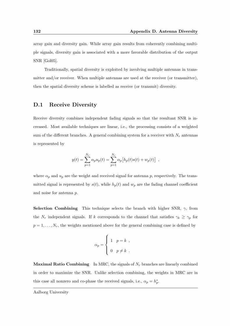
132 Appendix D. Antenna Diversity
array gain and diversity gain. While array gain results from coherently combining multi-
ple signals, diversity gain is associated with a more favorable distribution of the output
SNR [Gol05].
Traditionally, spatial diversity is exploited by involving multiple antennas in trans-
mitter and/or receiver. When multiple antennas are used at the receiver (or transmitter),
then the spatial diversity scheme is labelled as receive (or transmit) diversity.
D.1 Receive Diversity
Receive diversity combines independent fading signals so that the resultant SNR is in-
creased. Most available techniques are linear, i.e., the processing consists of a weighted
sum of the different branches. A general combining system for a receiver with Nr antennas
is represented by
y(t) =
Nr∑
p=1
αpup(t) =
Nr∑
p=1
αp
[hp(t)s(t) + wp(t)
],
where αp and up are the weight and received signal for antenna p, respectively. The trans-
mitted signal is represented by s(t), while hp(t) and wp are the fading channel coefficient
and noise for antenna p.
Selection Combining This technique selects the branch with higher SNR, γ, from
the Nr independent signals. If k corresponds to the channel that satisfies γk ≥ γp for
p = 1, . . . , Nr, the weights mentioned above for the general combining case is defined by
αp =
1 p = k ,
0 p 6= k .
Maximal Ratio Combining In MRC, the signals of Nr branches are linearly combined
in order to maximize the SNR. Unlike selection combining, the weights in MRC are in
this case all nonzero and co-phase the received signals, i.e., αp = h∗p.
Aalborg University

D.2 Transmit Diversity 133
Equal Gain Combining Although MRC is optimal in terms of SNR, equal gain com-
bining is a simpler technique that co-phases the signals and combines with the same
weight. Therefore, it does not need the knowledge of the SNR. The weights are then
αp = exp[−jθp], where θp is the phase of the signal at antenna p.
D.2 Transmit Diversity
Transmit diversity is a reasonable choice for the downlink of a cellular system to increase
the robustness of the link. If channel knowledge is available at the receiver, closed-loop
schemes can extract array gain. However, in the following we assume no channel informa-
tion at the transmitter. Only open-loop schemes that exploit diversity gain are considered.
Combining STBC with OFDM provides spatial diversity gain over frequency selec-
tive fading channels. In effect, space-time coding is applied on blocks of data symbols
instead of processing individual symbols.
D.2.1 Space-Time Coding
STC is a hybrid technique that applies both space and time diversity in a combined
way [PNG03]. The most common form of STC used for diversity is STBC. STC was
first introduced by Alamouti [Ala98] when presenting a two branch transmitter diversity
scheme that achieves full diversity.
The STBC proposed in [Ala98] transmits two symbols over two antennas and two
symbol durations according to the transmit matrix:
S =
sn sn+1
s∗n+1 s∗n
.
Under the assumption of constant fading over two consecutive symbols, the scheme achieves
diversity order of two.
Extending the concept of STBC, Tarokh [TJC99] proposed transmission blocks for
more than two transmit antennas that achieve full diversity, such as the code for four
Daniel Vaz Pato Figueiredo

134 Appendix D. Antenna Diversity
antennas and spatial rate 3/4, i.e., three symbols are transmitted over a block of four
symbol periods:
S =
sn sn+1sn+2√
(2)
sn+2√(2)
s∗n+1 s∗nsn+2√
(2)− sn+2√
(2)
s∗n+2√(2)
s∗n+2√(2)
−sn−s∗n+sn+1−s∗n+1
2
−sn+1−s∗n+1+sn−s∗n2
s∗n+2√(2)
− s∗n+2√(2)
sn+1+s∗n+1+sn−s∗n2 − sn+s∗n+sn+1−s∗n+1
2
.
D.2.2 Space-Frequency Coding
Although STBC provides diversity in time-varying channels, it is not effective in scenarios
with fading constant over long periods. Another disadvantage of STBC is the inherent
latency, since the decoding process requires the system to wait until the full block is
received before decoding. This issue becomes more important as the encoding block size
increases.
In the frequency domain, the problems above mentioned are avoided. The same
concept of STBC codes can be implemented in space and frequency domain. In frequency
selective channels, combined with OFDM, SFBC maps the symbols into subcarriers in-
stead of time symbols. In one OFDM symbol, the scheme decodes the full block avoiding
the latency problem [LW00]. SFBC also performs better at higher speeds due to encod-
ing within one single OFDM symbol. Nevertheless, it suffers degradation if the channel
response is nearly constant in frequency, since there is no frequency diversity.
D.3 SNR Statistics
This section presents the statistics of the output SNR, or post-processing SNR, for various
MIMO schemes under Rayleigh fading.
The wireless channel is a flat fading channel varying in time according to Jakes
model. The channel is slowly time-varying, and it is assumed constant for the number
of consecutive symbols corresponding to the transmit diversity block size under analysis,
Aalborg University

D.3 SNR Statistics 135
e.g., two symbols for Alamouti scheme. The channel consists of a single tap flat fading
characterized by Rayleigh statistics.
In NLOS scenarios, it is common to use Rayleigh fading model to describe the wire-
less channel behavior. The channel coefficients, h, follow a complex Gaussian distribution
of zero mean and variance σ2h. Then, the channel amplitude, |h|, is Rayleigh distributed
as in (A.1). The power of the channel is given by p = |h|2, and follows an exponential
distribution [Pro01],
f(p) =1
σ2h
exp
[− p
σ2h
].
The SNR of the link relates to the transmit power and noise as γ = Es
N0|h|2. For a simpler
representation of the SNR statistics, we consider the noise and transmit signal to have
unitary powers, such that γ = |h|2. Consequently, the PDF of the SNR of a SISO link
follows an exponential distribution:
f(γ) =1
σ2h
exp
[− γ
σ2h
].
D.3.1 Spatial Diversity
This section presents the analytical distributions for the post-processing SNR when or-
thogonal spatial diversity schemes are considered. We assume Nt transmitters and Nr
receivers where appropriate, and the fading links are i.i.d. following Rayleigh statistics.
D.3.1.1 Maximal Ratio Combining
MRC is a diversity technique that maximizes SNR from the utilization of independent
fading channels. This method needs channel knowledge, since it consists in weighting
the symbols at each antenna by the conjugate of the channel coefficient. As the channel
knowledge is commonly assumed to be available at the receiver, this technique is usually
regarded as a receive diversity scheme. In a SIMO configuration, the post-processing SNR
Daniel Vaz Pato Figueiredo

136 Appendix D. Antenna Diversity
and the corresponding distribution are given by [Pro01]
γ =
Nr∑
p=1
|hp|2 ,
f(γ) =1
(Nr − 1)!(σ2h
)NrγNr−1 exp
[−γσ2h
]. (D.1)
D.3.1.2 Space Time Coding
Orthogonal STBC is an open-loop transmit diversity schemes that achieve full diversity
gain [Ala98, TJC99]. Since it assumes no knowledge of the channel, unlike MRC, it does
not bring array gain. Therefore, the average SNR keeps constant when increasing the
number of antennas. The post-processing SNR and its PDF are given by [BH01]
γ =1
Nt
Nt∑
q=1
|hq|2 ,
f(γ) =1
(Nt − 1)!(
σ2h
Nt
)NtγNt−1 exp
−γσ2h
Nt
. (D.2)
D.3.1.3 MIMO Spatial Diversity
When a MIMO link is used to extract diversity from the system, both STBC and MRC
diversity schemes are employed. The Nt antennas at the transmitter encode the signal
using STBC, without channel knowledge. The available power at the transmitter is equally
divided among the transmission antennas when implementing STBC. Furthermore, the
Nr received signals are combined with MRC, using channel knowledge ideally estimated at
the receiver. In this situation, the SNR of the signal is chi-square distributed with 2NtNr
degrees of freedom. The resulting γ and its PDF are then given by
γ =1
Nt
Nr∑
p=1
Nt∑
q=1
|hp,q|2 ,
f(γ) =
(Nt
σ2h
)NtNr γNtNr−1
(NtNr − 1)!exp
[−Ntγ
σ2h
]. (D.3)
Aalborg University

D.3 SNR Statistics 137
D.3.2 Spatial Multiplexing
A MIMO wireless link can also be used to create parallel data streams between the
transmitter and the receiver, i.e., SM. A simple MIMO spatial multiplexing scheme
can be achieved with the ZF receiver. This scheme forms min(Nt, Nr) parallel data
streams [PNG03] without channel knowledge at the transmitter, i.e., the available power
is equally divided among the transmitter antennas. Although there are more advanced
techniques to perform SM that achieve better performances, only ZF has a known expres-
sion for the PDF of the post-processing SNR of each stream. In a MIMO channel that
applies SM-ZF, the SNR of ith stream is as follows:
γi =1
Nt
1
[(HHH)−1]i,i,
where [.]i,i is the ith diagonal value of a matrix, and (.)H represents the hermitian of the
matrix. The SNR of each stream has a chi-square distribution with 2(Nr −Nt +1) degrees
of freedom [PNG03]:
f(γ) =1
(σ2h
Nt
)Nr−Nt+1(Nr −Nt)!
γNr−Nt exp
− γσ2h
Nt
. (D.4)
D.3.3 Antenna Selection
AS is a spatial diversity scheme usually considered at the transmitter side due to its low
feedback requirement. It uses partial CSI, i.e., an indication of the antenna with highest
channel gain. The post-processing SNR for AS with Nt antennas follows:
γ = max(γ1, ..., γNt) .
In perfect channel estimation and no delay conditions, the PDF of the resulting SNR
is obtained from second order statistics, i.e., through the derivative of the Cumulative
Distribution Function (CDF). Assuming that the channel at each branch is i.i.d., with
Daniel Vaz Pato Figueiredo

138 Appendix D. Antenna Diversity
PDF, fsiso(γ), and CDF, Fsiso(γ), the PDF of the resulting SNR is [Pro01]
Fas(γ) = (Fsiso)Nt ,
fas(γ) =∂Fas
∂γ= Ntfsiso(γ)(Fsiso(γ))
Nt−1
=Nt
σ2h
(1 − exp
[− γ
σ2h
])Nt−1
exp
[− γ
σ2h
].
Note that the expression for the SNR distribution can be written in a different form,
fas(γ) = Nt
Nt−1∑
q=0
(−1)qCNt−1q
1
σ2h
exp
− γσ2h
q+1
.
Aalborg University

Appendix E
Adaptation and Scheduling
This appendix introduces the concepts of two techniques to adapt the transmission on the
basis of the channel conditions. In adaptive modulation, the transmitter selects the con-
stellation size to modulate the symbols. In multiuser scheduling, the transmitter chooses
the user that should be use the channel.
E.1 Adaptive Modulation
The adaptation of the transmission parameters to the fading conditions can lead to an
increase in throughput, to the optimization of the transmit power, or to the reduction
of the probability of bit error. These results are achieved by using favorable channel
conditions to send higher data rates or to use lower power [Gol05].
Practical adaptive schemes select the modulation and coding applied to maximize
spectral efficiency, while maintaining a certain QoS measured over the probability of er-
ror. It was shown in [CG01] that the adaptation of both rate and power does not bring
significant advantage over the adaptation of only rate. Therefore, we describe an adaptive
modulation technique that has a constant transmit power and aims at not exceeding the
maximum instantaneous BER.
The adaptation of the rate can easily be done by changing the constellation size of
the modulation, while maintaining the same symbol rate of the system. In this study, we
139

140 Appendix E. Adaptation and Scheduling
0 5 10 15 20 25 3010
−6
10−5
10−4
10−3
10−2
10−1
100
BE
R
SNR (dB)
4 QAM16 QAM64 QAM256 QAM
SNR thresholds
Figure E.1: BER of M-ary QAM over flat fading channel and thresholds for instantaneousBER constraint
restrict the adaptation to a discrete set of M-QAM orders. Owing to an easier practical
implementation, we limit the selection to the group of square constellations.
The target of the adaptation is to maintain the instantaneous BER lower than a
defined value, BER(γ) ≤ BERt. Thus, the system needs to estimate the BER performance
with respect to the SNR of the link. The discrete rate adaptation divides the SNR range
into R+1 regions to select one of the R constellation sizes available. Each modulation order
Mi is chosen when the SNR falls into region i delimited by SNR thresholds (or switching
thresholds), γi. Each region corresponds to the interval [γi, γi+1[. The thresholds are the
values of SNR that indicate the transition to a higher modulation available while keeping
the BER under the constraint, as shown in Figure E.1.
The switching thresholds can be obtained following a theoretical or a simulation
approach. The latter requires a numerical inspection of simulation results to identify the
threshold values for each modulation size individually. A theoretical approach that can
be generalized to any size of modulation is thus more appealing.
To find an expression of the SNR thresholds with respect to the BERt, we need to
invert the expression of BER performance. As mentioned in Appendix A, the BER for
Aalborg University

E.2 Multiuser Scheduling 141
M-QAM with Gray bit mapping is approximated as [Pro01]
PM−QAMb ≈ 2
log2M
[1 − 1√
M
]erfc
(√3
2(M − 1)
Es
N0
).
This expression is not easily invertible; therefore, the thresholds can not be described in
a closed-form solution. Thus, we use the approximation proposed in [CG01] for M-QAM,
M = 2ki ≥ 4 with Gray bit mapping and constant transmit power
BER(γi) ≈ c1 exp
−c2γi
1∫∞
γ0f(γ)dγ
2c3ki − c4
, 0 ≤ i ≤ R− 1 ,
where c1,2,3,4 are constants specific for the modulations employed. In the case of M-QAM,
M = 2ki ≥ 4, the constants are c1 = 0.2, c2 = 1.6, c3 = 1, and c4 = 1. Here, f(γ) is
the SNR distribution of the link. Considering a cut-off threshold of zero, i.e., γ0 = 0, the
system still transmits the lowest rate at the very low SNR. Then the BER approximation
reduces to
BER(γi) ≈ 0.2 exp
[−1.6γi
2ki − 1
], 0 ≤ i ≤ R− 1 .
Note that this approximation of BER is invertible and allows to present the thresholds in
a closed-form.
E.2 Multiuser Scheduling
In multiuser scenarios, the fact that each user has a different fading state at each moment
can be used by scheduling to increase the capacity of the system. Through opportunistic
scheduling, the BS selects the user that has the best channel at each time. A large number
of users combined with a large dynamic range of the fading channel variability boost the
gain obtained by MUD.
The two basic scheduling algorithms that deliver fairness or maximum throughput
are round-robin and maximum SNR schedulers. While these algorithms serve two contrary
goals, tradeoff schemes were proposed to achieve a balanced solution, from which we
Daniel Vaz Pato Figueiredo

142 Appendix E. Adaptation and Scheduling
selected proportional fair scheduler and opportunistic beamforming.
Round-robin Scheduler Also known as fair scheduler, the round-robin scheduler serves
all users in a sequential fashion, i.e., the user u to be allocated in slot n is found from
u = 1 + (n− 1) mod U ,
where U is the number of users in the system. This algorithm is independent of the
channel conditions and does not exploit MUD. On the other hand, it provides fairness
among users and achieves the best overall delay performance.
Maximum SNR Scheduler This scheme selects the user with the best SNR, γ, at
each slot, and attains the highest efficiency. The user u is scheduled in slot n if it satisfies
the condition
u = arg maxiγi(n) .
This scheduler achieves maximum MUD, i.e., the diversity order equals the number of
users in the system. However, it becomes impractical due to unfairness characteristic
among users experiencing different average SNR. In fact, users at low average SNR are
not allocated resources due to the poor channel conditions experienced, hence increasing
outage probability of the system.
Proportional Fair Scheduler This technique provides a tradeoff between maximum
MUD and fairness. The selection of the user to be served is based on the ratio of the
short-term SNR over the long term averaged SNR. This algorithm selects the user u to
be scheduled in slot n if
u = arg maxi
γi(n)
γi(n),
Aalborg University

E.2 Multiuser Scheduling 143
where γi(n) is the average SNR measured over a sliding window Tw
γi(n+ 1) =
(1 − 1Tw
)γi(n) + 1Twγi(n) , if user i is scheduled,
(1 − 1Tw
)γi(n) , if user i is not scheduled.
Opportunistic Beamforming If the channel experiences flat or slow fading, the maxi-
mum MUD scheduler transmits primarily to the users with better SNR condition. Instead
of using the proportional fair scheduler, fairness can be introduced with an antenna array
that produces random channel fluctuations. This artificial increase of channel variability
was proposed by [VTL02] and is referred to as Opportunistic Beamforming. This tech-
nique sees fast fading not as a source of unreliability, but as a randomization tool that
allows users to receive transmission slots when experiencing high SNR.
Daniel Vaz Pato Figueiredo

Appendix F
Statistics of SNR and Analytical
BER Using Prediction
This appendix describes the process followed to obtain the closed-form expressions of the
BER and SNR thresholds presented in Chapter 3. After proposing an unbiased predictor
for adaptive modulation, the author in [Ekm02] derives analytical expressions for the
BER performance of SISO flat fading channels. In this appendix, we extend the analytical
formulations to other MIMO schemes, spatial diversity, multiplexing, and AS.
The remainder of the appendix is organized as follows. Section F.1 introduces the un-
biased predictor. Section F.2 derives the conditional distributions of the true and predicted
SNR based on known Rayleigh channel statistics of Section D.3. Then, the conditional
distributions are used in Section F.3 to derive the expressions of BER performance.
F.1 Unbiased Power Predictor
The power predictor proposed in [Ekm02] is based on a prediction of the channel coeffi-
cients at instant n − L, to be applied at instant n, i.e., hn|n−L. The true power of the
145

146 Appendix F. Statistics of SNR and Analytical BER Using Prediction
channel and the SNR at instant n are defined as
pn = |hn|2 ,
γn = |hn|2Es
N0.
The average channel power is defined as σ2h = E[|hn|2], while the average SNR is given by
γ = E[|hn|2]Es
N0.
The predictor is based on past observations of the channel coefficients. The instanta-
neous predicted SNR at time n with horizon L, γn|n−L, and the predicted complex channel
gain, hn|n−L, are given by
γn|n−L = pn|n−LEs
σ2h
,
hn|n−L = Hpilotn−Lθ ,
where θ is the predictor vector and Hpilotn−L is the regressor vector with m observations of
the channel, Hpilotn−L =
[h
pilotn−L,h
pilotn−L−m, ...,h
pilotn−L−(k−1)m
]. The observations are affected by
an additive estimation error, hpilotn = hn + en.
In an adaptive modulation scheme, the transmission is adjusted through the value
of SNR at the time of transmission, and not through the channel gain, h. The use of the
squared amplitude of the predictor as a predictor for the channel power, pb = |h|2, results
in a biased estimate [Ekm02].
The unbiased quadratic power predictor described in [Ekm02, ESA02] is obtained
as follows:
p =∣∣∣Hpilot
n−Lθ∣∣∣2+ σ2
h − E[|hn|n−L|2
]. (F.1)
The criterion to choose the predictor vector θ was a Wiener adjustment. This
method ensures the optimal linear predictor in the MSE sense. It is shown in [Ekm02],
that the θ optimal in MSE sense for the channel predictor, also ensures an MSE optimal
Aalborg University

F.2 Distribution of Predicted SNR for MIMO 147
power predictor. Thus, the optimal adjustment for both cases reads
θ = R−1
Hpilotn−L
rhH
pilotn−L
,
rhH
pilotn−L
= E[hnH
pilotn−L
],
RH
pilotn−L
= E
[H
pilotn−L
(H
pilotn−L
)H].
When the predictor vector is optimally adjusted, the channel gain prediction error, ǫh =
hn − hn, and the power prediction error, ǫp = pn − pn, have variances:
σ2ǫh
= σ2h + (rhHpilot)HR−1
Hpilotn−L
rhHpilot ,
σ2ǫp
= (ǫh)2 +
∣∣∣∣(rhHpilot)HR−1
Hpilotn−L
rhHpilot
∣∣∣∣2
.
From (F.1), the optimal unbiased quadratic power predictor can be expressed in
terms of MSE-optimal linear channel predictor as
pn|n−L =∣∣∣hn|n−L
∣∣∣2+ σ2
h − σ2h
=∣∣∣hn|n−L
∣∣∣2+ σ2
ǫh.
Therefore, the unbiased power predictor reduces to
pn|n−L = |hn|n−L|2 + σ2ǫh
. (F.2)
In the derivations obtained for the predictor, an important variable to introduce is
the relative variance of the prediction error,
υhǫh =σ2
ǫh
σ2h
. (F.3)
F.2 Distribution of Predicted SNR for MIMO
The statistical distribution of the channel power is known for each MIMO scheme and is
shown in Section D.3. However, when using a predictor, an error between the predicted
Daniel Vaz Pato Figueiredo

148 Appendix F. Statistics of SNR and Analytical BER Using Prediction
value of the power and the true power of the channel changes the PDF of the SNR.
Therefore, here we derive the conditional probability of the true SNR given the predicted
SNR.
F.2.1 SISO
A Rayleigh channel is assumed, and an unbiased quadratic power predictor is applied with
optimized parameters, as described in Appendix F.1. The true SNR experienced by the
channel, and the prediction with horizon L, are represented by γn and γn|n−L, respectively.
The time subscripts of the variables are dropped to simplify the expressions.
The derivation of the following expressions for SISO case are detailed in [ESA02].
Although only the main results are presented for SISO, the intermediate steps can be
obtained substituting the number of antennas to one in the derivations of the SM or
MIMO diversity.
Using the distribution of SNR in Appendix D.3, and the power prediction mecha-
nism, the PDF of the predicted SNR, γ, is given by [Ekm02]
f(γ) =U (γ − γυhǫh)
γ (1 − υhǫh)exp
[− γ − γυhǫh
γ (1 − υhǫh)
], (F.4)
where U(.) is the Heaviside function, and υhǫh is the relative variance of the prediction
error.
F.2.1.1 Conditional PDF for True and Predicted SNR
The PDF of the true SNR, γ, conditioned on the predicted SNR, γ, is
f(γ|γ) =U(γ)U (γ − γυhǫh)
γυhǫh
exp
[−γ + γ − γυhǫh
γυhǫh
]I0
(2
γυhǫh
√γ (γ − γυhǫh)
), (F.5)
where I0 is the zero order modified Bessel function of first kind, defined as
I0(z) =∞∑
k=0
(14z
2)k
(k!)2.
Aalborg University

F.2 Distribution of Predicted SNR for MIMO 149
F.2.2 Spatial Multiplexing
A similar approach as described in [Ekm02] was followed to determine the expressions for
links using multiple antennas both at transmitter and receiver and employing SM with
ZF receiver.
Consider a Rayleigh fading channel, an SM system, with Nt transmit antennas, Nr
receive antennas and a ZF receiver. As shown in Appendix D.3.2, the true power of each
of the streams is a random variable with a PDF given by a chi-square distribution with
2(Nr −Nt + 1) degrees of freedom and the power shared by all transmit antennas:
f(p) =U(p)
(σ2h
Nt
)Nr−Nt+1(Nr −Nt)!
pNr−Nt exp
− pσ2h
Nt
.
Consider the configurations with the same number of antennas at receiver and trans-
mitter, i.e., Nr = Nt = Na. In this case, if the links are independent, the spatial rate is
Na. Thus, the PDF of true power of each stream follows a chi-square distribution with
two degrees of freedom:
f(p) =U(p)
σ2h
Na
exp
− pσ2h
Na
.
Since the predicted channel coefficients are weighted sums of zero-mean complex
Gaussian random variables, they also follow a zero-mean complex Gaussian distribu-
tion [TAG99]. Thus, the predicted power is also chi-square distributed. Using the defini-
tion of the biased predicted power, pb, in terms of the unbiased predictor, i.e., pb = p−σ2ǫh
,
one obtains the distribution of the unbiased predictor,
f(p) =U(p− σ2
ǫh)
σ2h−σ2
ǫh
Na
exp
−p− σ2
ǫhσ2h−σ2
ǫh
Na
.
Applying the transformation of variables γ = γ pσ2h
, dγdp = γ
σ2h
, the PDF of the pre-
Daniel Vaz Pato Figueiredo

150 Appendix F. Statistics of SNR and Analytical BER Using Prediction
dicted SNR, γ, reads
f(γ) =fp(γ
pσ2h
)
dγdp
=U(γ − γυhǫh)
γ(
1−υhǫh
Na
) exp
[− γ − γυhǫh
γNa
(1 − υhǫh)
].
F.2.2.1 Conditional PDF for True and Predicted SNR
Since both true and predicted power of the channel are exponentially distributed, their
joint PDF is given by the bivariate of the chi-square distribution with two degrees of
freedom [Ekm02, TAG99]. The bivariate distribution is written as
f(y1, y2) = α1 exp
[−α2
(y1
σ21
+y2
σ22
)]I0 (α3
√y1y2) , (F.6)
where I0 is the modified Bessel function of zero order and the constants αi are given, for
y1 = h and y2 = h, as follows:
α1 =1
σ2hσ
2h− |r
hh|2 , (F.7a)
α2 =σ2hσ
2h
σ2hσ
2h− |r
hh|2 , (F.7b)
α3 =2|r
hh|
σ2hσ
2h− |r
hh|2 . (F.7c)
If the predictor coefficients are MSE optimal, as described in Appendix F.1, then rhh
=
σ2h
= σ2h − σ2
ǫh, and the constants in (F.7) simplify to
α1 =1
σ2ǫh
(σ2h − σ2
ǫh), (F.8a)
α2 =σ2h
σ2ǫh
, (F.8b)
α3 =2
σ2ǫh
. (F.8c)
Aalborg University

F.2 Distribution of Predicted SNR for MIMO 151
Using (F.8) in (F.6), the joint distribution of the true and predicted power with an
SM system can be expressed as
f(p, p) =U(p)U(p− σ2
ǫh)
σ2ǫh
(σ2h − σ2
ǫh)
exp
− σ2h
σ2ǫh
pσ2h
Na
−p− σ2
ǫhσ2h−σ2
ǫh
Na
I0(
2Na
σ2ǫh
√p(p− σ2
ǫh)
).
Then, the conditional PDF of the true power conditioned to the predicted power value is
f(p|p) =f(p, p)
f(p)
=U(p)U(p− σ2
ǫh)
σ2ǫh
Na
exp
−p+ p− σ2
ǫhσ2
ǫh
Na
I0(
2Na
σ2ǫh
√p(p− σ2
ǫh)
).
Applying the transformation of variables γ = γ pσ2h
, the PDF of the SNR conditioned
on the predicted SNR, is given by
f(γ|γ) =fpp
(γ p
σ2h
|γ pσ2h
)
dγdp
=U(γ)U(γ − γυhǫh)
γNaυhǫh
exp
[−γ + γ − γυhǫh
γNaυhǫh
]I0
(2Na
γυhǫh
√γ(γ − γυhǫh)
). (F.9)
F.2.3 MIMO Diversity
In this section, the analysis of SNR statistics using a predictor is extended to the MIMO
diversity technique. We consider a configuration of multiple antennas at the transmitter,
where the signal is encoded via STBC, and multiple antennas at the receiver, where the
signal is combined through MRC.
As shown in Appendix D.3.1, in a Rayleigh fading channel, the true power of the
signal at the receiver is distributed according to a chi-square distribution with 2NtNr
degrees of freedom:
f(p) =U(p)
(σ2h
Nt
)NtNr
(NtNr − 1)!
pNtNr−1 exp
− pσ2h
Nt
. (F.10)
Daniel Vaz Pato Figueiredo

152 Appendix F. Statistics of SNR and Analytical BER Using Prediction
The definition of biased predicted power applied to the MIMO diversity case is
written as
pb =
∑Nt
q=1
∑Nr
p=1 |hq,p|2
Nt,
thus, the biased predicted power given in terms of the unbiased predictor is represented
as follows:
pb = p−∑Nt
q=1
∑Nr
p=1 σ2ǫhq,p
Nt.
Assuming the channel gain prediction error to be the same for all the links involved, the
predictor reduces to pb = p − Nrσ2ǫh
. Substituting this expression in (F.10), the PDF of
the unbiased predictor is
f(p) =U(p−Nrσ
2ǫh
)(
σ2h−σ2
ǫh
Nt
)NtNr
(NtNr − 1)!
(p−Nrσ2ǫh
)NtNr−1 exp
−p−Nrσ
2ǫh
σ2h−σ2
ǫh
Nt
.
Now, applying a transformation of variables γ = γ pσ2h
,
f(γ) =fp(γ
pσ2h
)
dγdp
=U(γ −Nrγυhǫh)
γ(
1−υhǫh
Nt
)NtNr
(NtNr − 1)!
(γσ2h
γ−Nrσ
2ǫh
)NtNr−1
exp
[− γ −Nrγυhǫh
γNt
(1 − υhǫh)
]
=U(γ −Nrγυhǫh)
(γNt
(1 − υhǫh))NtNr
(NtNr − 1)!
(γ −Nrγυhǫh)NtNr−1 exp
[− γ −Nrγυhǫh
γNt
(1 − υhǫh)
].
F.2.3.1 Conditional PDF for True and Predicted SNR
In MIMO diversity channel model, to obtain the joint PDF of the true power and pre-
dicted power, one needs to apply the bivariate of the chi-square distribution with 2NtNr
degrees of freedom. Since the chi-square distribution is a particular case of the gamma
distribution, a bivariate gamma distribution can be used. However, the two-dimensional
gamma distribution does not have a unique solution. The authors in [SAT82] proposed a
solution for the bivariate of the gamma distribution, known as SAT (Smith, Adelfang and
Aalborg University

F.2 Distribution of Predicted SNR for MIMO 153
Tubb) bivariate. This expression is also used in the context of channel prediction by the
authors in [Hol02, OHH04].
As the chi-square distribution is a particular case of the gamma distribution, the
bivariate of the chi-square distribution with 2NtNr degrees of freedom is
f(x1, x2) = α1(x1x2)NtNr−1
2 exp
[−α2
(x1
σ21
+x2
σ22
)]INtNr−1(α3
√x1x2) , (F.11)
where Iβ(z) is the modified Bessel function of order β. The constants αi are defined as
follows:
α1 =1
(σ21σ
22)
NtNr−12 (1 − ρ)ρ
NtNr−12 (NtNr − 1)!
, (F.12a)
α2 =1
1 − ρ, (F.12b)
α3 =2√ρ
1 − ρ
1√σ2
1σ22
, (F.12c)
where ρ =|rx1x2 |2
σ21σ2
2, and rx1x2 is the coefficient of correlation between the two random
variables. Inserting ρ in (F.12), and assuming the variables x1 and x2 to be replaced by
the true channel, h, and the predicted channel, h, the constants can be written as
α1 =1
(σ2hσ
2h)
NtNr−12 (1 − |r
hh|2
σ2hσ2h
)
(|r
hh|2
σ2hσ2h
)NtNr−12
(NtNr − 1)!
, (F.13a)
α2 =σ2hσ
2h
σ2hσ
2h− |r
hh|2 , (F.13b)
α3 =2|r
hh|
σ2hσ
2h− |r
hh|2 . (F.13c)
If the predictor coefficients are MSE optimal, as described in Appendix F.1, then
Daniel Vaz Pato Figueiredo

154 Appendix F. Statistics of SNR and Analytical BER Using Prediction
rhh
= σ2h
= σ2h − σ2
ǫh, and the constants in (F.13) simplify to
α1 =1
(σ2h(σ2
h − σ2ǫh
))NtNr+1
2 υhǫh(1 − υhǫh)NtNr−1
2 (NtNr − 1)!, (F.14a)
α2 =σ2h
σ2ǫh
, (F.14b)
α3 =2
σ2ǫh
. (F.14c)
Inserting (F.14) into (F.11), the joint distribution of the true and predicted power
with a STBC-MRC system results
f(p, p) =α1
(p(p−Nrσ
2ǫh
))NtNr−1
2 exp
− pσ2
ǫh
Nt
− σ2h
σ2ǫh
p−Nrσ2ǫh
σ2h−σ2
ǫh
Nt
×INtNr−1
(2
σ2ǫh
√p(p−Nrσ2
ǫh)
)U(p)U(p−Nrσ
2ǫh
) .
Therefore, the distribution of the true power of the channel conditioned to the predicted
power value is
f(p|p) =f(p, p)
f(p)
=U(p)U(p−Nrσ
2ǫh
)
υhǫh(σ2h)
NtNr+12 (σ2
h − σ2ǫh
)−NtNr−1
2 (1 − υhǫh)NtNr−1
2
×pNtNr−1
2 (p−Nrσ2ǫh
)NtNr−1
2 exp
−p+ p−Nrσ
2ǫh
σ2ǫh
Nt
INtNr−1
(2
σ2ǫh
√p(p−Nrσ2
ǫh)
).
(F.15)
Applying the transformation of variables γ = γ pσ2h
to (F.15), the PDF of the SNR γ
Aalborg University

F.2 Distribution of Predicted SNR for MIMO 155
conditioned on the predicted SNR, γ, is written as
f(γ|γ) =fpp
(γ p
σ2h
|γ pσ2h
)
dγdp
=U(γ)U(γ −Nrγυhǫh)Nt
γυhǫh
γNtNr−1
2 (γ −Nrγυhǫh)−NtNr−1
2
× exp
[−γ + γ −Nrγυhǫh
γNtυhǫh
]INtNr−1
(2Nt
γυhǫh
√γ(γ −Nrγυhǫh)
). (F.16)
F.2.4 Antenna Selection
In this section, the analysis of SNR statistics using a predictor is extended to the AS
technique. We consider a configuration of two antennas at the transmitter, and a selector
that chooses the highest SNR link at each instant based on feedback.
Appendix D.3.3 shows that the PDF of the post-processing SNR for AS can be
obtained from the SISO case by higher order statistics. Based on the results for SISO in
Appendix F.2.1, one obtains the distributions for the AS with two antennas as follows:
fas(γ) =2fsiso(γ)Fsiso(γ)
=U(γ − γυhǫh)2
γ(1 − υhǫh)exp
[− γ − γυhǫh
γ(1 − υhǫh)
](1 − exp
[− γ − γυhǫh
γ(1 − υhǫh)
]).
Now, with the results of the SISO case for joint distribution of SNR, we derive the
Daniel Vaz Pato Figueiredo

156 Appendix F. Statistics of SNR and Analytical BER Using Prediction
conditional PDF for AS:
fas(γ|γ) =2fsiso(γ, γ)Fsiso(γ, γ)
2fsiso(γ)Fsiso(γ)= fsiso(γ|γ)Fsiso(γ|γ)
=U(γ)U(γ − γυhǫh)1
γexp
[−γ + γ − γυhǫh
γυhǫh
]I0
(2
γυhǫh
√γ(γ − γυhǫh)
)
×(
1 − exp
[− γ − γυhǫh
γ(1 − υhǫh)
])−1 ∞∑
k=0
(1 − υhǫh)k
×(
1 − exp
[− γ
γυhǫh
] k∑
n1
1
n1!
(γ
γυhǫh
)n1)
×(
1 − exp
[− γ − γυhǫh
γ(1 − υhǫh)
] k∑
n2=0
1
n2!
(γ − γυhǫh
γυhǫh(1 − υhǫh)
)n2)
. (F.17)
F.3 M-QAM Performance
Using the distribution functions of the previous section, we show here the derivation of the
BER performance of M-QAM for the different MIMO cases considered, SISO, multiplexing,
diversity, and AS. Here, we aply the approximation of the BER given in Appendix E.1,
i.e.,
BER(γ, γ) ≈ 0.2 exp
[ −1.6γ
M(γ) − 1
],
where M(γ) ≡Mi.
F.3.1 SISO
In the context of the results in Appendix F.2, the authors in [Ekm02] derive the BER
expression as a function of the predicted SNR. With (F.5) in (3.6), one obtains the
instantaneous BER as a function of γ derived for the SISO case:
BER(γ) =
∫ ∞
0BER(γ, γ)f(γ|γ)dγ
=U(γ − γυhǫh)a(γ)
b(i)exp
[c(γ)2
4b(γ)
], (F.18)
Aalborg University

F.3 M-QAM Performance 157
where
a(γ) =0.2
γυhǫh
exp
[− γ − γυhǫh
γυhǫh
],
b(i) =1
γυhǫh
+1.6
Mi − 1,
c(γ) =2
γυhǫh
√γ − γυhǫh .
In the derivation of (F.18), two known results are employed:
exp(x) =∞∑
k=0
xk
k!, (F.19a)
∫ ∞
0xk exp(−αx) =
k!
αk+1. (F.19b)
It is also possible to write the instantaneous BER in (F.18) in the following form:
BER(γ) = U(γ − γυhǫh)0.2
γυhǫhb(i)exp
[γ − γυhǫh
γυhǫh
(1
γυhǫhb(i)− 1
)], (F.20)
where b(i) = 1γυhǫ
h
+ 1.6Mi−1 . Expressed in this closed-form, the BER expression (F.20)
can be used to obtain the predicted SNR required to achieve a defined BER. Thus, for
a system with instantaneous BER constraint, i.e., BER ≤ BERt, the SNR thresholds are
given by
γi = γυhǫh +γυhǫh(1
γυhǫh
b(i) − 1) ln
[BERt
0.2γυhǫhb(i)
]. (F.21)
The authors in [FSES04] also propose an expression for the SNR thresholds in the
situation of instantaneous BER constraint and constant power at transmitter for SISO.
After some manipulation it is possible to show that the expression in (F.21) is equivalent
to the result found in [FSES04, Equation (41)].
F.3.2 Spatial Multiplexing
Based on the results of the predicted SNR statistics for the SM configuration in Ap-
pendix F.2.2, we derive the instantaneous BER as a function of the predicted SNR. Hence,
Daniel Vaz Pato Figueiredo

158 Appendix F. Statistics of SNR and Analytical BER Using Prediction
inserting (F.9) into (3.6), one obtains the instantaneous BER as a function of γ derived
for SM with equal number of transmit and receive antennas as follows:
BER(γ) =
∫ ∞
0BER(γ, γ)f(γ|γ)dγ
= U(γ − γυhǫh)0.2Na
γυhǫhb(i)exp
[γ − γυhǫh
γNaυhǫh
(Na
γυhǫhb(i)− 1
)], (F.22)
where b(i) = Na
γυhǫh
+ 1.6Mi−1 .
Moreover, for a system with instantaneous BER constraint BER ≤ BERt, and
constant transmit power, the SNR thresholds are given by
γi = γυhǫh +γυhǫh
Na
(Na
γυhǫh
b(i) − 1) ln
[BERt
0.2
γυhǫhb(i)
Na
]. (F.23)
F.3.3 MIMO Diversity
This section describes the derivation of a closed-form of the BER as a function of the
predicted SNR in the MIMO diversity case. Inserting (F.16) into (3.6), and using the
properties (F.19), we calculate the instantaneous BER as a function of γ derived for the
MIMO diversity:
BER(γ) =
∫ ∞
0BER(γ, γ)f(γ|γ)dγ
= U(γ −Nrγυhǫh)0.2
(Nt
γυhǫhb(i)
)NtNr
exp
[γ −Nrγυhǫh
γNtυhǫh
(Nt
γυhǫhb(i)− 1
)],
(F.24)
where b(i) = Nt
γυhǫh
+ 1.6Mi−1 .
For a system with instantaneous BER constraint, BER ≤ BERt, and constant trans-
mit power, the SNR thresholds are given by
γi = Nrγυhǫh +γυhǫh
Nt
(Nt
γυhǫh
b(i) − 1) ln
[BERt
0.2
(γυhǫhb(i)
Nt
)NtNr
]. (F.25)
Aalborg University

F.3 M-QAM Performance 159
F.3.4 Antenna Selection
For a two branch AS system, we use the result shown in Appendix F.2.4. Thus, after
substituting (F.17) in (3.6), the expression of the instantaneous BER as a function of the
predicted SNR is written as
BER(γ) ≈U(γ − γυhǫh)0.2
γ
(1 − exp
[− γ − γυhǫh
γ(1 − υhǫh)
])−1
×∞∑
k=0
(1 − υhǫh)kΓlower
(γ−γυhǫ
h
γυhǫh(1−υhǫ
h) , k + 1
)
Γ(k + 1)
×(
1
β + 1σ2
ǫh
exp
[− γ − γυhǫh
γυhǫh + 1β
]− 1
β + 2σ2
ǫh
exp
[− γ − γυhǫh
γυhǫh
]
×k∑
n1=0
(1
βσ2ǫh
+ 2
)n1 Γupper
(γ−γυhǫ
h
γυhǫh(1−υhǫ
h) , k + 1
)
Γ(n1 + 1)
), (F.26)
where β = 1.6Mi−1 , Γ(n) is the complete gamma function, Γlower(x, n) is the lower tail of the
incomplete gamma function, and Γupper(x, n) is the upper tail of the incomplete gamma
function.
Since (F.26) is not in a closed-form, and no other closed-form solutions are known
for the BER performance of AS in function of the predicted SNR, it is not possible to
analytically obtain the SNR thresholds. Nevertheless, the tractable equation obtained for
the BER performance allows for a numerical evaluation of the performance.
Daniel Vaz Pato Figueiredo


Appendix G
Link Simulator EUTRA
The link-level simulator used in Sections 2.3 and 5.2 was initially developed by the Ph.D.
students at Aalborg University: Akhilesh Pokhariyal, Basuki Priyanto, Christian Rom,
and Na Wei, as well as Claudio Rosa and Frank Frederiksen from Nokia Siemens Networks.
A more detailed description of the simulator can be found in [WPR+06], as well as in the
Ph.D. dissertations [Pok07, Wei07].
The block diagram of the link-level chain of the simulator is shown in Figure G.1.
This is a single-user downlink simulation where the data generation assumes that there
is always data to transmit. The stream of bits to transmit is Cyclic Redundancy Check
(CRC) encoded, divided into several blocks, and passed to the channel encoder. The
UTRA Release 6 Turbo coding and rate matching algorithm are then applied. After in-
terleaving, the bits are modulated with QAM followed by a bit remapping to place the
systematic bits at more reliable constellation points [WPR+06]. The modulated sym-
bols are then passed to the MIMO space-frequency encoder. The SFC depends on the
MIMO scheme selected, and it is at this block that one of the contributions of this thesis
was introduced by implementing several MIMO encoding schemes, including UTOD and
ABBA [TBH00] schemes, and extending the encoding from two to four transmit antennas.
An Inverse Fast Fourier Transform (IFFT) is applied on each transmit antenna
branch, and CP is added before the convolution with the multipath MIMO channel. The
161

162 Appendix G. Link Simulator EUTRA
Data source BER and BLER
CRCattachment
CRCverification
Code blocksegmentation
Code blockdesegmentation
Channel codingRate matching
Channel decodingRate dematching
Interleaver Deinterleaver
QAM mapping QAM demapping
MIMO S-F processing
MIMO S-F processing
Multipath MIMO channel
IFFTInsert CP
FFTRemove CP
Figure G.1: Block diagram of link-level simulator
Aalborg University

163
MIMO channel model is based on the contribution of [SKF+01] for the I-METRA project
which has been used and validated in [Ber05]. The MIMO channel matrix with uncorre-
lated spatial links is pre-generated for the number of transmitters and receivers configu-
ration to save simulation time.
The noise and interference in Section 2.3 are modeled with AWGN. However, in Sec-
tion 5.2, the other cell interference is not modeled as AWGN, and the contribution of this
thesis is the extension of the downlink simulator to consider simultaneous transmissions
from other BSs according to the pathloss model and ISD.
The continuous time-varying impulse response channel model is too complex for a
simple analysis. Therefore, a discrete time tapped delay limitation is employed to model
the wideband multipath model. The resolution of the sampling depends on the bandwidth
of the transmitted signal. In 3GPP, the delay of the l path is quantized in time to the
nearest 1/16th chip interval Tc = 13.84µs.
The receiver estimates the channel for each spatial link, and the channel estimation
is assumed to be perfect. After removing the CP and passing the time domain signal
through the FFT, the signal is passed to the MIMO decoder. The MIMO decoder block
equalizes the transmitted symbols. Then, the inverse process to obtain the data bits is
done to measure the BER and BLER.
Based on the channel estimation, the system applies link adaptation at the trans-
mitter. The link adaptation mechanism selects the MCS based on the averaged received
SNR. Particularly, the scheme adapts among QPSK, 16-QAM, and 64-QAM, as well as
different coding rates ranging from 1/6 and up to 4/5. The Exponential Effective SNR
Mapping (EESM) model is applied to obtain an effective SNR value for prediction of the
BLER on the basis of a set of link-level AWGN performance curves. The link adaptation
targets a maximum BLER of 20%.
The above described procedure is applied to the data generated for a frame of seven
OFDM symbols. The simulations are then run for a total of 3000 frames, and we validate
the BER curves with the number of errors before and after the coding process. The number
Daniel Vaz Pato Figueiredo

164 Appendix G. Link Simulator EUTRA
of uncoded bit transmitted amounts to approximately 40 million (7 OFDM symbols in a
frame; 1024 data subcarriers; and QPSK modulation). As an example, in Figure 2.8, the
fixed modulation SFC at 20 dB results in 4495 uncoded errors with 16-QAM, whereas LDC
results in more than half million errors with QPSK. After channel coding, the number
of coded bit errors drops to levels below tens of errors for very high SNR, which does
not allow for a plotting of coded BER curves. The spectral efficiency curves are directly
dependent on the coded BER and BLER, but are little affected by errors in their exact
values, since the performance is mainly driven by the maximum achievable throughput at
high SNR.
Aalborg University

Appendix H
Dissemination of Results
During the Ph.D. studies, the following publications in technical peer-reviewed conferences
and journals have been generated:
• Muhammad I. Rahman, Ragnar V. Reynisson, Daniel V.P. Figueiredo, and Ramjee
Prasad, “Coordinated Sub-Carrier and Band Hopping in OFDMA based Systems,”
to appear in Special Issue of Wireless Personal Communications (WPC) Journal,
Springer, 2008.
• Daniel V.P. Figueiredo, Zihuai Lin, and Troels B. Sørensen, “Performance of Linear
Dispersion Codes with Linear Receivers,” in Proc. International Symposium on
Wireless Personal Multimedia Communications (WPMC), Jaipur, India, December
2007.
• Daniel V.P. Figueiredo, Zihuai Lin, and Troels B. Sørensen, “Average Error Proba-
bility of MIMO Diversity Systems in the Presence of Multiple Interferers,” in Proc.
IEEE International Symposium on Wireless Communication Systems (ISWCS), Trond-
heim, Norway, October 2007.
• Muhammad I. Rahman, Ragnar V. Reynisson, Daniel V.P. Figueiredo, and Ram-
jee Prasad, “Coordinated Sub-Carrier and Band Hopping in OFDMA based Sys-
tems,” in Proc. IEEE International Symposium on Wireless Communication Sys-
165

166 Appendix H. Dissemination of Results
tems (ISWCS), Trondheim, Norway, October 2007.
• Daniel V.P. Figueiredo, and Elisabeth de Carvalho, “Switching Thresholds for Rate
Adaptation with MRC under Feedback Delay,” in Proc. International Symposium on
Wireless Personal Multimedia Communications (WPMC), San Diego, USA, Septem-
ber 2006.
• Daniel V.P. Figueiredo, Elisabeth de Carvalho, and Luc Deneire, “Impact of Feed-
back Delay on Rate Adaptation for Multiple Antenna Systems,” in Proc. IEEE
International Symposium on Personal, Indoor and Mobile Radio Communications
(PIMRC), Helsinki, Finland, September 2006.
• Daniel V.P. Figueiredo, Muhammad I. Rahman, Nicola Marchetti, Frank H.P. Fitzek,
Marcos D. Katz, Youngkwon Cho, and Ramjee Prasad, “Transmit Diversity vs
Beamforming for Multi-user OFDM Systems,” in Proc. International Symposium
on Wireless Personal Multimedia Communications (WPMC), Abano Terme, Italy,
June 2004.
Moreover, the collaboration with industry in the projects JADE and IST-SURFACE
led to the certification of one patent, and the co-authoring of several project deliverables.
Patents
• Daniel V.P. Figueiredo, Elisabeth de Carvalho, Luc Deneire, Sung-Ryul Yun, David
Mazzarese, and Sung-Kwon Hong, “Transmission Strategies for Downlink Multi-User
OFDMA,” Samsung, Korean Patent KR2006-0021584, March 8, 2006.
Project Deliverables
• Troels B. Sørensen, Daniel V.P. Figueiredo, Yuanye Wang, Wsewolod Warzanskyj,
et al., “Description of the Network Optimal Transmit and Receive,” IST-SURFACE
Deliverable D5, December 2007.
Aalborg University

167
• Antonio Fasano, Sergio Barbarossa, Loreto Pescosolido, Gesualdo Scutari, Luis G.
Ordones, Eduardo Calvo, Javier R. Fonollosa, Alba Pages-Zamora, Troels B. Sørensen,
Daniel V.P. Figueiredo, Istvan Z. Kovacs, et al., “Preliminary Design of the Multi-
user Optimal Transmit and Receive Strategy,” IST-SURFACE Deliverable D4, De-
cember 2006.
• Daniel V.P. Figueiredo, Elisabeth de Carvalho, and Luc Deneire, “Transmission
Strategies in MIMO Scenarios with Channel Prediction,” JADE project deliverable
PD-WP1-1-Jun06-MIMOSwicthing, Aalborg University, Denmark, June 2006.
• Daniel V.P. Figueiredo, Elisabeth de Carvalho, and Luc Deneire, “Transmission
Strategies in MIMO Scenarios with Channel Prediction,” JADE project deliverable
PD-WPB-WA2-Dec05-swicthing, Aalborg University, Denmark, December 2005.
• Muhammad I. Rahman, Ragnar V. Reynisson, and Daniel V.P. Figueiredo, “Sub-
carrier and Band Hopped Orthogonal Frequency Division Multiple Access (SCBH-
OFDMA),” JADE project deliverable TN-WPB-WA4-Oct05, Aalborg University,
Denmark, October 2005.
• Daniel V.P. Figueiredo, Elisabeth de Carvalho, and Luc Deneire, “Transmission
Strategies in Multi-user Scenarios,” JADE project deliverable TN-WPB-WA2-Oct05,
Aalborg University, Denmark, October 2005.
• Muhammad I. Rahman, Huan C. Nguyen, Daniel V.P. Figueiredo, Ragnar V. Reynis-
son, and Elisabeth de Carvalho, “Initial Recommendations for Access Techniques
and Duplexing for Cellular Systems,” JADE project deliverable B-2005-06-2, Aal-
borg University, Denmark, June 2005.
• Megumi Kaneko, Nicola Marchetti, and Daniel V.P. Figueiredo, “Multi-user Diver-
sity in Scheduling,” JADE project deliverable D3.2[2], Aalborg University, Denmark,
January 2005.
• Muhammad I. Rahman, Nicola Marchetti, Daniel V.P. Figueiredo, Huan C. Nguyen,
Daniel Vaz Pato Figueiredo

168 Appendix H. Dissemination of Results
Ragnar V. Reynisson, and Seshaiah Ponnekanti, “Multi-antenna Techniques in Multi-
user OFDM Systems,” JADE project deliverable D3.2[1],Aalborg University, Den-
mark, September 2004.
• Muhammad I. Rahman, Søren S. Christian, Suvra S. Das, Basak Can, Ragnar V.
Reynisson, Anders B. Olsen, Jesper M. Kristensen, Nicola Marchetti, Daniel V.P.
Figueiredo, and Petar Popovski, “Comparison of Various Modulation and Access
Schemes under Ideal Channel Conditions,” JADE project deliverable D3.1[1], Aal-
borg University, Denmark, July 2004.
Aalborg University

Bibliography
[3GP06a] 3GPP, “Physical layer aspects for evolved Universal Terrestrial Radio Access
(UTRA),” Technical Specification TR 25.814 (V7.1.0), September 2006.
[3GP06b] ——, “Requirements for Evolved UTRA (E-UTRA) and Evolved UTRAN
(E-UTRAN),” Technical Specification TR 25.913 (V7.3.0), March 2006.
[3GP07] ——, “Spatial Channel Model for Multiple Input Multiple Output (MIMO)
simulations,” Technical Specification TR 25.996 (V7.0.0), June 2007.
[AG00] M. S. Alouini and A. J. Goldsmith, “Adaptive modulation over nakagami
fading channels,” Kluwer Journal on Wireless Personal Communications,
vol. 13, no. 1, pp. 119–143, 2000.
[Ala98] S. M. Alamouti, “A simple transmit diversity technique for wireless com-
munications,” IEEE Journal on Selected Areas in Communications, vol. 16,
no. 8, pp. 1451–1458, 1998.
[And05] J. G. Andrews, “Interference cancellation for cellular systems: a contempo-
rary overview,” IEEE Wireless Communications Magazine, vol. 12, no. 2,
pp. 19–29, 2005.
[App76] S. Applebaum, “Adaptive arrays,” IEEE Transactions on Antennas and
Propagation, vol. 24, no. 5, pp. 585–598, 1976.
[AR01] Y. Akyildiz and B. D. Rao, “Statistical performance analysis of optimum
combining with co-channel interferers and flat Rayleigh fading,” in Proc.
169

170 BIBLIOGRAPHY
IEEE Global Communications Conference (GLOBECOM), vol. 6, San An-
tonio, TX, USA, November 2001, pp. 3663–3667.
[B06] H. Bolcskei, Space-Time Wireless Systems: From Array Processing to MIMO
Communications, D. Gesbert, C. Papadias, and A.-J. van der Veen, Eds.
New York, NY, USA: Cambridge University Press, 2006.
[Bar04] S. Barbarossa, “Trace-orthogonal design of MIMO systems with simple scalar
detectors, full diversity and (almost) full rate,” in Proc. IEEE Workshop on
Signal Processing Advances in Wireless Communications (SPAWC), Lisbon,
Portugal, July 2004, pp. 308–312.
[Ber05] L. Berger, “Performance of Multi-Antenna Enhanced HSDPA,” Ph.D. dis-
sertation, Aalborg University, Denmark, 2005.
[BH01] G. Bauch and J. Hagenauer, “Analytical evaluation of space-time transmit
diversity with FEC-coding,” in Proc. IEEE Global Communications Confer-
ence (GLOBECOM), vol. 1, San Antonio, TX, USA, November 2001, pp.
435–439.
[BKRM+03] L. T. Berger, T. E. Kolding, J. Ramiro-Moreno, P. Ameigeiras, L. Schu-
macher, and P. E. Mogensen, “Interaction of transmit diversity and pro-
portional fair scheduling,” in Proc. IEEE Vehicular Technology Conference
(VTC), vol. 4, Jeju, Korea, April 2003.
[BZR05] J. P. Burke, J. R. Zeidler, and B. D. Rao, “CINR difference analysis of
optimal combining versus maximal ratio combining,” IEEE Transactions on
Wireless Communications, vol. 4, no. 1, pp. 1–5, 2005.
[CA03] C. Chayawan and V. A. Aalo, “Average error probability of digital cellular
radio systems using MRC diversity in the presence of multiple interferers,”
IEEE Transactions on Wireless Communications, vol. 2, no. 5, pp. 860–864,
2003.
Aalborg University

BIBLIOGRAPHY 171
[Car86] A. B. Carlson, Communication Systems. New York, NY, USA: McGraw-
Hill, 1986.
[CEGHJ02] S. Catreux, V. Erceg, D. Gesbert, and R. W. Heath Jr, “Adaptive mod-
ulation and MIMO coding for broadband wireless data networks,” IEEE
Communications Magazine, vol. 40, no. 6, pp. 108–115, 2002.
[CFD+06] E. D. Carvalho, D. V. P. Figueiredo, L. Deneire, S.-R. Yun, D. Maz-
zarese, and S.-K. Hong, “Transmission Strategies for Downlink Multi-User
OFDMA,” Korean Patent KR2006-0 021 584, March 8, 2006.
[CFS97] J. Cui, D. D. Falconer, and A. U. H. Sheikh, “Performance evaluation of opti-
mum combining and maximal ratio combining in the presence of co-channel
interference and channel correlation for wireless communication systems,”
Mobile Networks and Applications, vol. 2, no. 4, pp. 315–324, 1997.
[CG01] S. T. Chung and A. J. Goldsmith, “Degrees of freedom in adaptive modula-
tion: a unified view,” IEEE Transactions on Communications, vol. 49, no. 9,
pp. 1561–1571, 2001.
[CJS07] G. Caire, N. Jindal, and S. Shamai, “On the required accuracy of transmitter
channel state information in multiple antenna broadcast channels,” in Proc.
Asilomar Conference on Signals, Systems and Computers, Pacific Grove, CA,
USA, November 2007, pp. 287–291.
[CLH01] S. T. Chung, A. Lozano, and H. C. Huang, “Low complexity algorithm for
rate and power quantization in extended V-BLAST,” in Proc. IEEE Vehic-
ular Technology Conference (VTC), vol. 2, Atlantic City, NJ, USA, October
2001.
[Col07] S. R. Colas, “Channel Modelling and SINR Evaluation in MBMS for LTE,”
Master’s thesis, Aalborg University, 2007.
Daniel Vaz Pato Figueiredo

172 BIBLIOGRAPHY
[CS99] J. Cui and A. U. H. Sheikh, “Outage probability of cellular radio systems
using maximal ratio combining in the presence of multiple interferers,” IEEE
Transactions on Communications, vol. 47, no. 8, pp. 1121–1124, 1999.
[DB05] M. Ding and S. Blostein, “Low-feedback adaptive-rate MIMO spatial multi-
plexing with zero forcing detection,” in Canadian Workshop on Information
Theory, Edmonton, Canada, 2005.
[DTB02] M. O. Damen, A. Tewfik, and J. C. Belflore, “A construction of a space-time
code based on number theory,” IEEE Transactions on Information Theory,
vol. 48, no. 3, pp. 753–760, 2002.
[Ekm02] T. Ekman, “Prediction of Mobile Radio Channels: Modeling and Design,”
Ph.D. dissertation, Uppsala University, Sweden, 2002.
[ESA02] T. Ekman, M. Sternad, and A. Ahlen, “Unbiased power prediction of
Rayleigh fading channels,” in Proc. IEEE Vehicular Technology Conference
(VTC), vol. 1, Vancouver, Canada, September 2002, pp. 280–284.
[FB06] A. Fasano and S. Barbarossa, “Iterative MMSE decoder for trace-orthogonal
space-time coding,” in Proc. IEEE International Conference on Acoustics,
Speech, and Signal Processing (ICASSP), vol. 4, Toulouse, France, May 2006.
[FC06] D. V. P. Figueiredo and E. D. Carvalho, “Switching thresholds for rate
adaptation with MRC under feedback delay,” in Proc. International Sym-
posium on Wireless Personal Multimedia Communications (WPMC), San
Diego, CA, USA, September 2006.
[FCD06] D. V. P. Figueiredo, E. D. Carvalho, and L. Deneire, “Impact of feedback
delay on rate adaptation for multiple antenna systems,” in Proc. IEEE Inter-
national Symposium on Personal, Indoor and Mobile Radio Communications
(PIMRC), Helsinki, Finland, September 2006.
Aalborg University

BIBLIOGRAPHY 173
[Fla03] “OFDM for Mobile Data Communications,” Online Tutorial, Whitepaper,
Flarion Technologies, March 2003.
[FLS07a] D. V. P. Figueiredo, Z. Lin, and T. B. Sørensen, “Average error probabil-
ity of MIMO diversity systems in the presence of multiple interferers,” in
Proc. IEEE International Symposium on Wireless Communication Systems
(ISWCS), Trondheim, Norway, October 2007.
[FLS07b] ——, “Performance of linear dispersion codes with linear receivers,” in Proc.
International Symposium on Wireless Personal Multimedia Communications
(WPMC), Jaipur, India, December 2007.
[Fos96] G. J. Foschini, “Layered space-time architecture for wireless communication
in a fading environment when using multiple antennas,” Bell Labs Technical
Journal, vol. 1, no. 2, pp. 41–59, 1996.
[FPKHJ05] A. Forenza, A. Pandharipande, H. K., and R. W. Heath Jr, “Adaptive MIMO
transmission scheme: exploiting the spatial selectivity of wireless channels,”
in Proc. IEEE Vehicular Technology Conference (VTC), vol. 5, Stockholm,
Sweden, May 2005, pp. 3188–3192.
[FRM+04] D. V. P. Figueiredo, M. I. Rahman, N. Marchetti, F. H. P. Fitzek, M. D.
Katz, Y. Cho, and R. Prasad, “Transmit diversity vs beamforming for multi-
user OFDM systems,” in Proc. International Symposium on Wireless Per-
sonal Multimedia Communications (WPMC), Abano Terme, Italy, Septem-
ber 2004.
[FSES04] S. Falahati, A. Svensson, T. Ekman, and M. Sternad, “Adaptive modulation
systems for predicted wireless channels,” IEEE Transactions on Communi-
cations, vol. 52, no. 2, pp. 307–316, 2004.
[God04] L. Godara, Smart Antennas. Boca Raton, FL, USA: CRC Press, Inc., 2004.
Daniel Vaz Pato Figueiredo

174 BIBLIOGRAPHY
[Goe99] D. L. Goeckel, “Adaptive coding for time-varying channels using outdated
fading estimates,” IEEE Transactions on Communications, vol. 47, no. 6,
pp. 844–855, 1999.
[Gol05] A. J. Goldsmith, Wireless Communications. New York, NY, USA: Cam-
bridge University Press, 2005.
[GSS+03] D. Gesbert, M. Shafi, D. Shiu, P. Smith, and A. Naguib, “From theory to
practice: an overview of MIMO space-time coded wireless systems,” IEEE
Journal on Selected Areas in Communications, vol. 21, no. 3, pp. 281–302,
2003.
[HG03] L. He and H. Ge, “A new full-rate full-diversity orthogonal space-time block
coding scheme,” IEEE Communications Letters, vol. 7, no. 12, pp. 590–592,
2003.
[HH02] B. Hassibi and B. M. Hochwald, “High-rate codes that are linear in space
and time,” IEEE Transactions on Information Theory, vol. 48, no. 7, pp.
1804–1824, 2002.
[HJL05] R. W. Heath Jr and D. J. Love, “Multimode antenna selection for spatial
multiplexing systems with linear receivers,” IEEE Transactions on Signal
Processing, vol. 53, no. 8, pp. 3042–3056, 2005.
[HJP02] R. W. Heath Jr and A. J. Paulraj, “Linear dispersion codes for MIMO
systems based on frame theory,” IEEE Transactions on Signal Processing,
vol. 50, no. 10, pp. 2429–2441, 2002.
[HJP05] ——, “Switching between diversity and multiplexing in MIMO systems,”
IEEE Transactions on Communications, vol. 53, no. 6, pp. 962–968, 2005.
[HMT04] B. M. Hochwald, T. L. Marzetta, and V. Tarokh, “Multiple-antenna chan-
nel hardening and its implications for rate feedback and scheduling,” IEEE
Transactions on Information Theory, vol. 50, no. 9, pp. 1893–1909, 2004.
Aalborg University

BIBLIOGRAPHY 175
[Hol02] H. Holm, “Adaptive Coded Modulation Performance and Channel Estima-
tion Tools for Flat Fading Channels,” Ph.D. dissertation, Norwegian Univer-
sity of Science and Technology, Trondheim, Norway, 2002.
[HP03] S. Hara and R. Prasad, Multicarrier Techniques for 4G Mobile Communica-
tions. Norwood, MA, USA: Artech House, Inc., 2003.
[HT01] J. Heiskala and J. Terry, OFDM Wireless Lans: A Theoretical and Practical
Guide. Indianapolis, IN, USA: Sams Publishing, 2001.
[HT04] H. Holma and A. Toskala, WCDMA for UMTS: Radio Access for Third
Generation Mobile Communications. New York, NY, USA: John Wiley &
Sons, Inc., 2004.
[HT06] ——, HSDPA/HSUPA for UMTS: High Speed Radio Access for Mobile Com-
munications. New York, NY, USA: John Wiley & Sons, Inc., 2006.
[IEE04] IEEE Standard for Local and Metropolitan Area Networks Part 16: Air In-
terface for Fixed Broadband Wireless Access Systems, IEEE Std. 802.16-2004,
October 2004.
[IEE06] IEEE Standard for Local and Metropolitan Area Networks Part 16: Air Inter-
face for Fixed Broadband Wireless Access Systems, IEEE Std. 802.16e-2005,
February 2006.
[ITU97] “Guidelines for evaluation of radio transmission technologies for IMT-2000,”
ITU-R, Recommendations M.1225, 1997.
[JC94] W. C. Jakes and D. C. Cox, Microwave Mobile Communications. Wiley-
IEEE Press, 1994.
[JSC+07] M. Jordan, M. Senst, Y. Cui, G. Ascheid, and H. Meyr, “Downlink based in-
tercell time synchronization using maximum likelihood estimation,” in Proc.
IST Mobile and Wireless Communications Summit, Budapest, Hungary, July
2007, pp. 1–5.
Daniel Vaz Pato Figueiredo

176 BIBLIOGRAPHY
[KH95] R. Knopp and P. A. Humblet, “Information capacity and power control in
single-cell multiuser communications,” in Proc. IEEE International Confer-
ence on Communications (ICC), vol. 1, Seatlle, WA, USA, June 1995.
[Kim02] B. Kim, “Smart Base Station Antenna Performance for Several Scenarios -
an Experimental and Modeling Investigation,” Ph.D. dissertation, Virginia
Polytechnic Institute and State University, Blacksburg, VA, USA, 2002.
[KMAH02] K. Kopsa, G. Matz, H. Artes, and F. Hlawatsch, “Space-time synchronization
algorithms for UMTS/TDD systems with strong co-channel interference,”
in Proc. IEEE Global Communications Conference (GLOBECOM), vol. 1,
Taipei, Taiwan, November 2002, pp. 254–258.
[KT03] Y. Ko and C. Tepedelenlioglu, “Space-time block coded rate-adaptive mod-
ulation with uncertain SNR feedback,” in Proc. Asilomar Conference on
Signals, Systems and Computers, vol. 1, Pacific Grove, CA, USA, November
2003, pp. 1032–1036.
[KVC02] P. Kyritsi, R. A. Valenzuela, and D. C. Cox, “Channel and capacity esti-
mation errors,” IEEE Communications Letters, vol. 6, no. 12, pp. 517–519,
2002.
[LLC02] V. K. N. Lau, Y. Liu, and T. A. Chen, “Optimal multi-user space time
scheduling for wireless communications,” in Proc. IEEE Vehicular Technol-
ogy Conference (VTC), vol. 4, Vancouver, Canada, September 2002.
[LR99] J. C. Liberti and T. S. Rappaport, Smart Antennas for Wireless Communi-
cations: IS-95 and Third Generation CDMA Applications. Upper Saddle
River, NJ, USA: Prentice Hall PTR, 1999.
[LS99] Y. Li and N. R. Sollenberger, “Adaptive antenna arrays for OFDM sys-
tems with cochannel interference,” IEEE Transactions on Communications,
vol. 47, no. 2, pp. 217–229, 1999.
Aalborg University

BIBLIOGRAPHY 177
[LW00] K. F. Lee and D. B. Williams, “A space-frequency transmitter diversity tech-
nique for OFDM systems,” in Proc. IEEE Global Communications Confer-
ence (GLOBECOM), vol. 3, San Francisco, CA, USA, November 2000, pp.
1473–1477.
[LZW06] J. Liu, J. K. Zhang, and K. M. Wong, “On the Design of Minimum BER
Linear Space-Time Block Codes for MIMO Systems Equipped with MMSE
Receivers,” IEEE Transactions on Signal Processing, vol. 54, no. 8, pp. 3147–
3158, 2006.
[MAT] Matlab - the language of technical computing. [Online]. Available:
http://www.mathworks.com/products/matlab/
[MG03] X. Ma and G. B. Giannakis, “Full-diversity full-rate complex-field space-
time coding,” IEEE Transactions on Signal Processing, vol. 51, no. 11, pp.
2917–2930, 2003.
[MKL06] J. Moon, J. Y. Ko, and Y. H. Lee, “A framework design for the next-
generation radio access system,” IEEE Journal on Selected Areas in Com-
munications, vol. 24, no. 3, pp. 554–564, 2006.
[MS98] J. Medbo and P. Schramm, “Channel models for HIPERLAN/2 in different
indoor scenarios,” COST 259 TD(98)70, ETSI BRAN, Bradford, UK, April
1998.
[NAP04] H. T. Nguyen, J. B. Andersen, and G. F. Pedersen, “Capacity and perfor-
mance of MIMO systems under the impact of feedback delay,” in Proc. IEEE
International Symposium on Personal, Indoor and Mobile Radio Communi-
cations (PIMRC), vol. 1, Barcelona, Spain, September 2004.
[NH04] S. Nagaraj and Y.-F. Huang, “Multiple antenna transmission with channel
state information: a low-rate feedback approach,” IEEE Signal Processing
Letters, vol. 11, no. 6, pp. 573–576, June 2004.
Daniel Vaz Pato Figueiredo

178 BIBLIOGRAPHY
[NP00] R. V. Nee and R. Prasad, OFDM for Wireless Multimedia Communications.
Norwood, MA, USA: Artech House, Inc., 2000.
[OHH04] G. E. Oien, H. Holm, and K. J. Hole, “Impact of channel prediction on adap-
tive coded modulation performance in Rayleigh fading,” IEEE Transactions
on Vehicular Technology, vol. 53, no. 3, pp. 758–769, 2004.
[Par00] J. D. Parsons, The Mobile Radio Propagation Channel. New York, NY,
USA: John Wiley & Sons, Inc., 2000.
[Pat03] M. Patzold, Mobile Fading Channels. New York, NY, USA: John Wiley &
Sons, Inc., 2003.
[PNG03] A. J. Paulraj, R. Nabar, and D. Gore, Introduction to Space-Time Wireless
Communications. New York, NY, USA: Cambridge University Press, 2003.
[Pok07] A. Pokhariyal, “Downlink Frequency-Domain Adaptation and Scheduling - A
Case Study Based on the UTRA Long Term Evolution,” Ph.D. dissertation,
Aalborg University, Denmark, 2007.
[PP97] A. J. Paulraj and C. B. Papadias, “Space-time processing for wireless com-
munications,” IEEE Signal Processing Magazine, vol. 14, no. 6, pp. 49–83,
1997.
[Pro01] J. G. Proakis, Digital Communication. New York, NY, USA: McGraw-Hill,
2001.
[Rah07] M. I. Rahman, “Channelization, Link Adaptation and Multi-antenna Tech-
niques for OFDM(A) Based Wireless Systems,” Ph.D. dissertation, Aalborg
University, Denmark, 2007.
[Rap96] T. S. Rappaport, Wireless Communications: Principles and Practice. Pis-
cataway, NJ, USA: IEEE Press, 1996.
Aalborg University

BIBLIOGRAPHY 179
[RDF04] M. I. Rahman, S. S. Das, and F. H. P. Fitzek, “OFDM Based WLAN Sys-
tems,” Aalborg University, Denmark, Tech. Rep. R-04-1002, January 2004.
[RG97] H. Rohling and R. Gruneid, “Performance comparison of different multiple
access schemes for the downlink of an OFDM communication system,” in
Proc. IEEE Vehicular Technology Conference (VTC), vol. 3, Phoenix, AZ,
USA, May 1997, pp. 1365–1369.
[SAT82] O. E. Smith, S. I. Adelfang, and J. D. Tubbs, “A Bivariate Gamma Prob-
ability Distribution with Application to Gust Modeling,” NASA Technical
Memorandum, vol. 82483, 1982.
[SBM+04] G. L. Stuber, J. R. Barry, S. W. McLaughlin, Y. E. G. Li, M. A. Ingram, and
T. G. Pratt, “Broadband MIMO-OFDM wireless communications,” Proceed-
ings of the IEEE, vol. 92, no. 2, pp. 271–294, February 2004.
[SH98] A. Shah and A. M. Haimovich, “Performance analysis of optimum combin-
ing in wireless communications with Rayleigh fading and cochannel interfer-
ence,” IEEE Transactions on Communications, vol. 46, no. 4, pp. 473–479,
1998.
[SH03] H. Schoeneich and P. A. Hoeher, “Single antenna interference cancellation:
iterative semi-blind algorithm and performance bound for joint maximum-
likelihood interference cancellation,” in Proc. IEEE Global Communications
Conference (GLOBECOM), vol. 3, San Francisco, CA, USA, December 2003.
[SKF+01] L. Schumacher, J. P. Kermoal, F. Frederiksen, K. I. Pedersen, A. Algans, and
P. E. Mogensen, “MIMO channel characterization,” IST-METRA Project
Deliverable 2, February 2001.
[SLWR01] A. Seeger, A. Lobinger, R. Wiedmann, and B. Raaf, “Downlink eigenbeam-
former with combining of eigenbeams,” in Proc. IEEE Global Communica-
Daniel Vaz Pato Figueiredo

180 BIBLIOGRAPHY
tions Conference (GLOBECOM), vol. 5, San Antonio, TX, USA, November
2001, pp. 1269–1273.
[SP04] N. Sharma and C. B. Papadias, “Full-rate full-diversity linear quasi-
orthogonal space-time codes for any number of transmit antennas,”
EURASIP Journal on Applied Signal Processing, vol. 2004, no. 9, pp. 1246–
1256, 2004.
[TAG99] X. Tang, M. S. Alouini, and A. J. Goldsmith, “Effect of channel estimation
error on M-QAM BER performance in Rayleigh fading,” IEEE Transactions
on Communications, vol. 47, no. 12, pp. 1856–1864, 1999.
[TBH00] O. Tirkkonen, A. Boariu, and A. Hottinen, “Minimal non-orthogonality rate
1 space-time block code for 3+ Tx antennas,” in Proc. IEEE International
Symposium on Spread Spectrum Techniques and Applications (ISSSTA),
vol. 2, Parsippany, NJ, USA, September 2000.
[Tel95] E. Telatar, “Capacity of multi-antenna gaussian channels,” AT&T-Bell Labs
Internal Tech. Memo., June 1995.
[THJ05] T. Tang and R. W. Heath Jr, “Space-time interference cancellation in MIMO-
OFDM systems,” IEEE Transactions on Vehicular Technology, vol. 54, no. 5,
pp. 1802–1816, 2005.
[TJC99] V. Tarokh, H. Jafarkhani, and A. R. Calderbank, “Space-time block cod-
ing for wireless communications: performance results,” IEEE Journal on
Selected Areas in Communications, vol. 17, no. 3, pp. 451–460, 1999.
[Ven03] R. Venkatasubramanian, “Beamforming for MC-CDMA,” Master’s thesis,
Virginia Polytechnic Institute and State University, Blacksburg, VA, USA,
2003.
[VTL02] P. Viswanath, D. N. C. Tse, and R. Laroia, “Opportunistic beamforming
Aalborg University

BIBLIOGRAPHY 181
using dumb antennas,” IEEE Transactions on Information Theory, vol. 48,
no. 6, pp. 1277–1294, 2002.
[Wei07] N. Wei, “MIMO Techniques in UTRA Long Term Evolution,” Ph.D. disser-
tation, Aalborg University, Denmark, 2007.
[WPR+06] N. Wei, A. Pokhariyal, C. Rom, B. E. Priyanto, F. Frederiksen, C. Rosa,
T. B. Sorensen, T. E. Kolding, and P. E. Mogensen, “Baseline E-UTRA
downlink spectral efficiency evaluation,” in Proc. IEEE Vehicular Technology
Conference (VTC), Montreal, Canada, September 2006, pp. 1–5.
[WSKM06] N. Wei, T. B. Sørensen, T. E. Kolding, and P. E. Mogensen, “Analysis
and evaluation of link adaptation including MIMO adaptation,” in Proc.
IEEE Vehicular Technology Conference (VTC), Montreal, Canada, Septem-
ber 2006, pp. 1–5.
[ZL03] Y. J. Zhang and K. B. Letaief, “Optimizing power and resource management
for multiuser MIMO/OFDM systems,” in Proc. IEEE Global Communica-
tions Conference (GLOBECOM), vol. 1, San Francisco, CA, USA, December
2003.
Daniel Vaz Pato Figueiredo


Vita
Daniel V.P. Figueiredo was born in 1980 in Lisbon, Portugal. He started university in 1998
and obtained the Licenciatura (5-year degree) in October 2003 in Electronics and Com-
puters Engineering at Instituto Superior Tecnico (IST), Technical University of Lisbon,
Portugal. In spring 2002, he spent one semester at Politecnico di Milano, Italy, as an ex-
change student with an ERASMUS scholarship. In February 2004, he joined the Wireless
Networking Group (WING) at the Institute of Electronic Systems, Aalborg University,
and he has been enrolled as a Ph.D. student from June 2004. Since August 2006, he is
with the Radio Access Technology (RATE) section of the Institute of Electronic Systems
at Aalborg University.
The main topics of research include spatial diversity and multiplexing, link adapta-
tion, and multicarrier systems. He has been actively engaged in IEEE volunteer activities,
co-organizing a number of events including the first and second occurrences of the interna-
tional conference Annual IEEE Student Paper Conference (AISPC’07 and AISPC’08).
Contact email: [email protected]
183