MPRAMunich Personal RePEc Archive

Black swan protection: an experimentalinvestigation

Andrea Morone and Ozlem Ozdemir

Univerista degli studi di Bari, Aldo Moro; Dipartimento di StudiAziendali e Giusprivatistici, Bari, Italy, Universitat Jaune I;Departament d’Economia, Castellon, Spain, Middle East TechnicalUniversity; Department of Business Administration, Ankara, Turkey

2012

Online at http://mpra.ub.uni-muenchen.de/38842/MPRA Paper No. 38842, posted 16. May 2012 13:37 UTC

1

Black Swan Protection: an Experimental Investigation

Ozlem Ozdemir (Corresponding Author) 1

Middle East Technical University, Department of Business Administration, Ankara, Turkey

Andrea Morone

Università degli Studi di Bari, Aldo Moro Dipartimento di Studi Aziendali e Giusprivatistici, Bari, Italy

And Universitat Jaune I

Departament d'Economia, Castellon, Spain Abstract

This experimental study investigates insurance decisions in low-probability, high-loss risk

situations. Results indicate that subjects consider the probability of loss (loss size) when they

make buying decisions (paying decisions). Most individuals are risk averse with no specific

threshold probability.

JEL Classification: C91 and D81

Keywords: Black swan, Risk, Insurance, Low probability, High loss, Experiment

1 Professor, Middle East Technical University (METU), Department of Business Administration, 06531 Ankara, Turkey, Phone: +90-312-210 3061, Fax: +90-312-210 7962, Email: yozlem@metu.edu.tr The authors gratefully acknowledge the financial support of the Max Planck Institute of Economics, Jena, Germany.

2

1. Introduction

The black swan (i.e. low probability and high loss; LPHL hereafter) events can be expressed as

risky situations where probability of occurrence is low, but the harmful effect can be very

dreadful (e.g., bankruptcy, insolvency, terrorism, and natural disasters). Both individuals and

firms implement different risk reduction mechanisms, such as life insurance, credit insurance,

home insurance, and storm shelters, against these events. However, how people decide to insure

specifically towards LPHL hazards is questionable. Theoretical frameworks concerning

protective measures chosen by individuals against LPHL risk situations have been developed

over the past thirty years (e.g., Arrow, 1996; Cook and Graham, 1975; Dong et al., 1996;

Kunreuther, 1979). Most have consistently demonstrated that insurance markets for high

probability events can be expressed by standard expected utility theory (EUT); however, the

EUT is inadequate to explain decision making processes in low probability risk situations

(Hershey and Schoemaker, 1980). As Morgenstern (1979) mentioned:

[T]he domain of our axioms on utility theory is also restricted….For example, the

probabilities used must be within certain plausible ranges and not go to 0.01 or

even less to 0.001, then be compared to other equally tiny numbers such as 0.02,

etc. (Morgenstern, 1979, p.178).

Most survey studies indicate that some people perceive the risk as if no hazard exists, while

others seem to react to the situation as if it is a frequent risk exposure condition (e.g. Camerer

and Kunreuther, 1989; McClelland et al., 1990; McDaniels et al., 1992; Slovic et al., 1980). The

reasons why individuals behave in two opposite ways have not attracted enough attention in the

literature. One possible reason might be that some people may take into account the low

probability of occurrence and react to LPHL risks as if there is no such risk, while others may

focus on the high loss and thus overreact (Etchart-Vincent, 2004). In fact, Sjöberg (1999) finds

3

that the demand for risk reduction is influenced by the severity of the hazard and not by the

probability. Yet, some other scholars conclude that people make insurance decisions based on

probability estimates (Slovic et al., 1977)2. The lack of a definite answer to the question of

whether individuals focus on low probability or high loss when they make insurance decisions in

LPHL situations, stresses the necessity for further empirical research.

The present study contributes to this research stream by conducting an experiment to

examine a dominant risk assessing consideration, namely, the probability of loss versus loss

amount on individuals’ insurance decisions in LPHL risky situations. During the course of this,

we investigate whether using different elicitation methods induces any change in these decisions.

In addition, we check the effects of individuals’ risk attitudes, their self-determined threshold

probabilities and their demographic characteristics (such as age, income and gender) on these

insurance valuations.

In our experiment, we use two different probabilities of loss (p=0.01 and 0.005)3 and two

loss amounts (all the income and half of the income) to test the dominance of probability and

size of losses on the insurance decision. Furthermore, the design allows us to answer whether the

two different elicitation mechanisms reported in the literature to detect the decision making

process induce similar risk mitigation behaviour. Specifically, we try to examine the differences

in individuals’ insurance decisions between the case when they are asked to decide whether they

want to buy the insurance or not (asking dichotomous questions to elicit an individual’s choice),

and the case when they are asked to state the amount of money they are willing to pay for the

insurance (asking open-ended questions to elicit an individual’s valuation). The theoretical

framework does not distinguish risk reduction mechanisms, such as insurance. However, 2 An alternative explanation could be that subjects behave according prospect theory in this case they will overestimate the probability in both cases to about the same larger value. 3 Note that “low” probability is mostly taken as 0.01 and less in the empirical literature (e.g., Camerer, 1995; McClelland et al., 1993, Ganderton et al., 2000).

4

according to the preference reversal phenomenon, individuals may consider different kinds of

information when they make choice versus pricing/valuation decisions (Grether and Plott, 1979;

Holt, 1986; Kagel and Roth, 1995, Segal, 1988; Tversky, Sattah, and Slovic, 1988; Tversky,

Slovic, and Kahneman, 1990). More specifically, when people make choices they focus on the

probability and when they assign values they look at the size of the outcome. Previous

experimental studies about LPHL risks investigate either buying insurance decisions or paying

for insurance decisions. To our knowledge there is no study that investigates both. According to

the most recent experimental study that utilises buying decisions (through asking dichotomous

questions) to examine insurance decisions in LPHL situations, the probability of occurrence of

the risky event plays a dominant role in valuing insurance (Ganderton et al., 2000). However,

another experimental study by McClelland et al. (1993) investigates insurance paying decisions

(using open-ended questions), and concluded that some individuals are willing to pay zero while

others are willing to pay much higher than the expected loss value. This contradiction

necessitates further research.

Moreover, our experimental design also allows us to elicit a threshold probability in

individuals’ minds and gauge their risk attitudes towards the effects of these insurance decisions.

A “threshold probability” is presented as the minimum probability in an individual’s mind for a

given amount of loss for which he/she buys insurance. Through eliciting individuals’ threshold

probabilities, we can also test the prospective reference theory, which suggests that people

overestimate the risk if the probability is below a particular threshold probability and

underestimate if it is above the threshold probability (Viscusi and Evans, 1990). We also

determine subjects’ risk attitudes by following the calculation used by McClelland et al. (1993).

This enables us to test the consistency of our results with the well known fourfold patterns of risk

attitudes (Di Mauro and Maffioletti, 2004). According to the well known fourfold patterns of risk

5

attitudes as suggested by Prospect Theory (Kahneman and Tversky, 1979), people are risk averse

for gains and risk seekers for losses in high probability events, and risk averse for losses and risk

seekers for gains in low probability events. Finally, in addition to the effects of threshold

probability and risk attitude, we examine how an individual’s endowment in the experiment,

gender, age and income influences his/her insurance buying and paying decisions.

The results of the current study are important for academicians and practitioners in the

insurance market in many aspects. It contributes to the literature by answering whether using

different methods to elicit individuals’ insurance valuations changes their decisions and affects

the dominant consideration of probability of loss and amount of loss. In other words, the study

answers the question “do individuals consider different kinds of information when they make

choice versus pricing insurance decisions?”. Further, it tests prospective reference theory through

asking individuals’ threshold probabilities in low-probability and high-loss risk context. The

practitioners in the insurance industry may use information about (1) the dominant consideration

of probability of loss versus size of loss on consumers’ decisions, (2) the minimum probability of

loss in their mind necessary to start considering insuring, (3) their risk attitudes and (4) the role

of gender, income and age on decisions for motivating society to mitigate LPHL risks (such as

natural disasters).

2. Experimental Method

96 subjects took part in the experiment. All of them first received a questionnaire asking their

demographic characteristics such as their age, gender and income before receiving written

instructions on the experiment.4 The experiment has two phases. The purpose of the first phase is

to give subjects a “hard earned income”, which they then had to protect in the second phase of

4 The original instructions were in German. Instructions in English are available upon request.

6

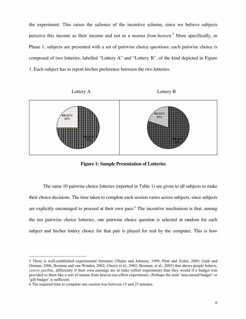
the experiment. This raises the salience of the incentive scheme, since we believe subjects

perceive this income as their income and not as a manna from heaven.5 More specifically, in

Phase 1, subjects are presented with a set of pairwise choice questions; each pairwise choice is

composed of two lotteries, labelled “Lottery A” and “Lottery B”, of the kind depicted in Figure

1. Each subject has to report his/her preference between the two lotteries.

Lottery A Lottery B

Figure 1: Sample Presentation of Lotteries

The same 10 pairwise choice lotteries (reported in Table 1) are given to all subjects to make

their choice decisions. The time taken to complete each session varies across subjects, since subjects

are explicitly encouraged to proceed at their own pace.6 The incentive mechanism is that, among

the ten pairwise choice lotteries, one pairwise choice question is selected at random for each

subject and his/her lottery choice for that pair is played for real by the computer. This is how

5 There is well-established experimental literature (Thaler and Johnson, 1999; Plott and Zeiler, 2005; Guth and Ortman, 2006; Bosman and van Winden, 2002; Cherry et al., 2002; Bosman, et al., 2005) that shows people behave, ceteris paribus, differently if their own earnings are at stake (effort experiment) than they would if a budget was provided to them like a sort of manna from heaven (no-effort experiment). (Perhaps the term ‘non-earned budget’ or ‘gift budget’ is sufficient. 6 The required time to complete one session was between 15 and 25 minutes.

300 ECU 75%

400 ECU 25%

300 ECU 80%

500 ECU 20%

7

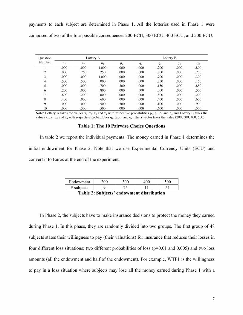
payments to each subject are determined in Phase 1. All the lotteries used in Phase 1 were

composed of two of the four possible consequences 200 ECU, 300 ECU, 400 ECU, and 500 ECU.

Question Number

Lottery A Lottery B p1 p2 p3 p4 q1 q2 q3 q4

1 .000 .000 1.000 .000 .000 .200 .000 .800 2 .000 .750 .250 .000 .000 .800 .000 .200 3 .000 .000 1.000 .000 .000 .700 .000 .300 4 .500 .500 .000 .000 .000 .850 .000 .150 5 .000 .000 .700 .300 .000 .150 .000 .850 6 .200 .000 .800 .000 .500 .000 .000 .500 7 .800 .200 .000 .000 .000 .800 .000 .200 8 .400 .000 .600 .000 .000 .400 .000 .600 9 .000 .000 .500 .500 .000 .100 .000 .900

10 .000 .500 .500 .000 .000 .600 .000 .500 Note: Lottery A takes the values x1, x2, x3 and x4 with respective probabilities p1, p2, p3 and p4 and Lottery B takes the values x1, x2, x3 and x4 with respective probabilities q1, q2, q3 and q4. The x vector takes the value (200, 300, 400, 500).

Table 1: The 10 Pairwise Choice Questions

In table 2 we report the individual payments. The money earned in Phase 1 determines the

initial endowment for Phase 2. Note that we use Experimental Currency Units (ECU) and

convert it to Euros at the end of the experiment.

Endowment 200 300 400 500 # subjects 9 25 11 51

Table 2: Subjects’ endowment distribution

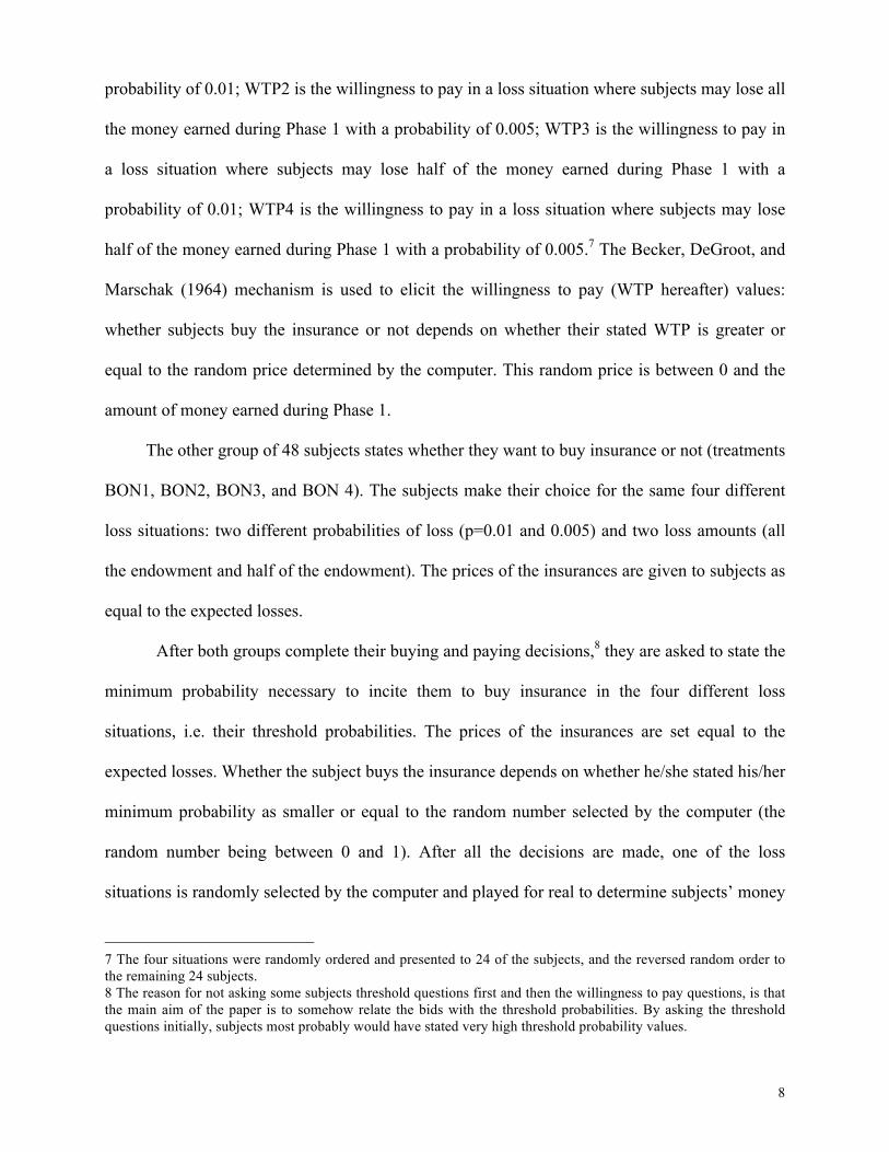
In Phase 2, the subjects have to make insurance decisions to protect the money they earned

during Phase 1. In this phase, they are randomly divided into two groups. The first group of 48

subjects states their willingness to pay (their valuations) for insurance that reduces their losses in

four different loss situations: two different probabilities of loss (p=0.01 and 0.005) and two loss

amounts (all the endowment and half of the endowment). For example, WTP1 is the willingness

to pay in a loss situation where subjects may lose all the money earned during Phase 1 with a

8

probability of 0.01; WTP2 is the willingness to pay in a loss situation where subjects may lose all

the money earned during Phase 1 with a probability of 0.005; WTP3 is the willingness to pay in

a loss situation where subjects may lose half of the money earned during Phase 1 with a

probability of 0.01; WTP4 is the willingness to pay in a loss situation where subjects may lose

half of the money earned during Phase 1 with a probability of 0.005.7 The Becker, DeGroot, and

Marschak (1964) mechanism is used to elicit the willingness to pay (WTP hereafter) values:

whether subjects buy the insurance or not depends on whether their stated WTP is greater or

equal to the random price determined by the computer. This random price is between 0 and the

amount of money earned during Phase 1.

The other group of 48 subjects states whether they want to buy insurance or not (treatments

BON1, BON2, BON3, and BON 4). The subjects make their choice for the same four different

loss situations: two different probabilities of loss (p=0.01 and 0.005) and two loss amounts (all

the endowment and half of the endowment). The prices of the insurances are given to subjects as

equal to the expected losses.

After both groups complete their buying and paying decisions,8 they are asked to state the

minimum probability necessary to incite them to buy insurance in the four different loss

situations, i.e. their threshold probabilities. The prices of the insurances are set equal to the

expected losses. Whether the subject buys the insurance depends on whether he/she stated his/her

minimum probability as smaller or equal to the random number selected by the computer (the

random number being between 0 and 1). After all the decisions are made, one of the loss

situations is randomly selected by the computer and played for real to determine subjects’ money

7 The four situations were randomly ordered and presented to 24 of the subjects, and the reversed random order to the remaining 24 subjects. 8 The reason for not asking some subjects threshold questions first and then the willingness to pay questions, is that the main aim of the paper is to somehow relate the bids with the threshold probabilities. By asking the threshold questions initially, subjects most probably would have stated very high threshold probability values.

9

balances at the end of the experiment. As noted previously, we use ECU and convert it to Euros

at the end of the experiment. Three randomly selected subjects have their ECUs converted to

Euros at the following exchange rate: 1ECU = €1, and for the others the rate is: 1 ECU = €0.02

(for example, for one person 500 ECU= €500, for others 500ECU = € 10).9

3. Results

The experiment was run at the Max Planck Institute of Economics laboratory, in Jena, Germany.

The computerized experiment software was developed in z-Tree (Fischbacher, 2007). Students

from Jena University were recruited to participate in the experiment using the ORSEE software

(Greiner, 2004). 45% of subjects were male and the average age was 23 (minimum 19 and

maximum 39). The average monthly income earned was 348 Euro (minimum 0 and maximum

1100 Euro). It is important to note that the data is available from the authors upon request.

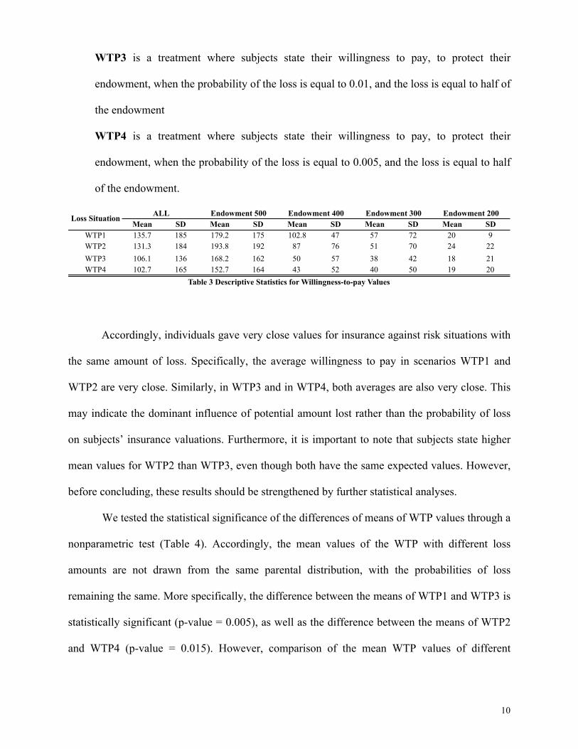
Table 3 represents the statistics for 48 individuals, stating their maximum willingness to

pay for the insurance (paying decisions) in four loss situations:

WTP1 is a treatment where subjects state their willingness to pay, to protect their

endowment, when the probability of the loss is equal to 0.01, and the loss is equal to all the

endowment;

WTP2 is a treatment where subjects state their willingness to pay, to protect their

endowment, when the probability of the loss is equal to 0.005, and the loss is equal to all

the endowment;

9 Many studies have used similar random incentive mechanisms (e.g., Starmer and Sugden, 1991; Hey and Lee, 2005; Drehmann et al., 2007; Laury, 2006).

10

WTP3 is a treatment where subjects state their willingness to pay, to protect their

endowment, when the probability of the loss is equal to 0.01, and the loss is equal to half of

the endowment

WTP4 is a treatment where subjects state their willingness to pay, to protect their

endowment, when the probability of the loss is equal to 0.005, and the loss is equal to half

of the endowment.

Accordingly, individuals gave very close values for insurance against risk situations with

the same amount of loss. Specifically, the average willingness to pay in scenarios WTP1 and

WTP2 are very close. Similarly, in WTP3 and in WTP4, both averages are also very close. This

may indicate the dominant influence of potential amount lost rather than the probability of loss

on subjects’ insurance valuations. Furthermore, it is important to note that subjects state higher

mean values for WTP2 than WTP3, even though both have the same expected values. However,

before concluding, these results should be strengthened by further statistical analyses.

We tested the statistical significance of the differences of means of WTP values through a

nonparametric test (Table 4). Accordingly, the mean values of the WTP with different loss

amounts are not drawn from the same parental distribution, with the probabilities of loss

remaining the same. More specifically, the difference between the means of WTP1 and WTP3 is

statistically significant (p-value = 0.005), as well as the difference between the means of WTP2

and WTP4 (p-value = 0.015). However, comparison of the mean WTP values of different

Mean SD Mean SD Mean SD Mean SD Mean SDWTP1 135.7 185 179.2 175 102.8 47 57 72 20 9WTP2 131.3 184 193.8 192 87 76 51 70 24 22WTP3 106.1 136 168.2 162 50 57 38 42 18 21WTP4 102.7 165 152.7 164 43 52 40 50 19 20

Loss Situation

Table 3 Descriptive Statistics for Willingness-to-pay Values

ALL Endowment 500 Endowment 400 Endowment 300 Endowment 200

11

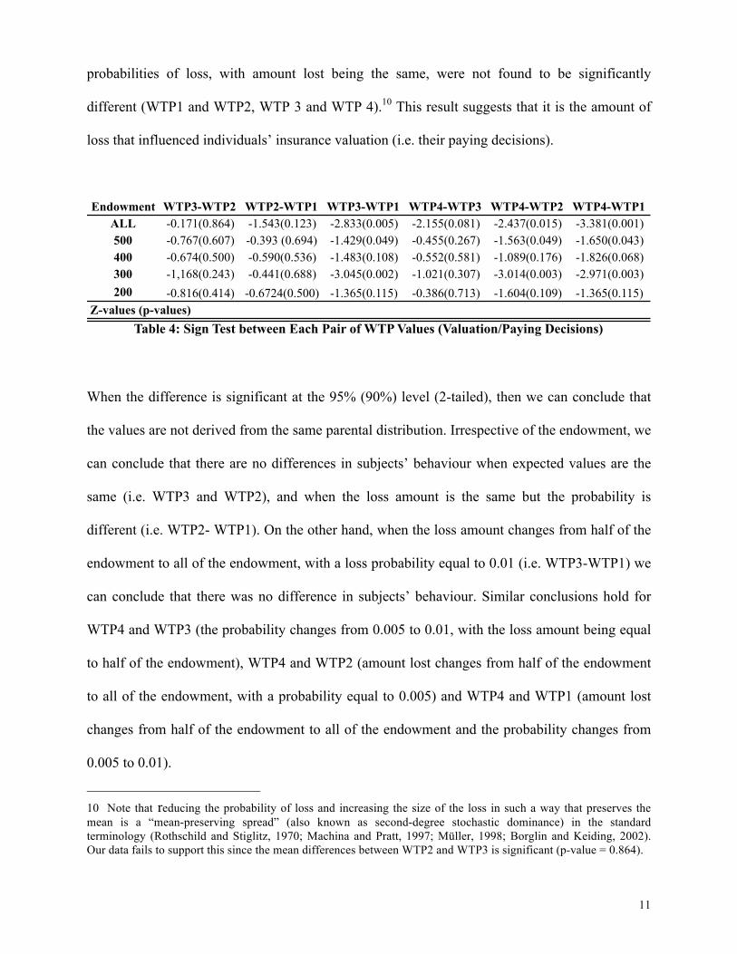
probabilities of loss, with amount lost being the same, were not found to be significantly

different (WTP1 and WTP2, WTP 3 and WTP 4).10 This result suggests that it is the amount of

loss that influenced individuals’ insurance valuation (i.e. their paying decisions).

When the difference is significant at the 95% (90%) level (2-tailed), then we can conclude that

the values are not derived from the same parental distribution. Irrespective of the endowment, we

can conclude that there are no differences in subjects’ behaviour when expected values are the

same (i.e. WTP3 and WTP2), and when the loss amount is the same but the probability is

different (i.e. WTP2- WTP1). On the other hand, when the loss amount changes from half of the

endowment to all of the endowment, with a loss probability equal to 0.01 (i.e. WTP3-WTP1) we

can conclude that there was no difference in subjects’ behaviour. Similar conclusions hold for

WTP4 and WTP3 (the probability changes from 0.005 to 0.01, with the loss amount being equal

to half of the endowment), WTP4 and WTP2 (amount lost changes from half of the endowment

to all of the endowment, with a probability equal to 0.005) and WTP4 and WTP1 (amount lost

changes from half of the endowment to all of the endowment and the probability changes from

0.005 to 0.01).

10 Note that reducing the probability of loss and increasing the size of the loss in such a way that preserves the mean is a “mean-preserving spread” (also known as second-degree stochastic dominance) in the standard terminology (Rothschild and Stiglitz, 1970; Machina and Pratt, 1997; Müller, 1998; Borglin and Keiding, 2002). Our data fails to support this since the mean differences between WTP2 and WTP3 is significant (p-value = 0.864).

Endowment WTP3-WTP2 WTP2-WTP1 WTP3-WTP1 WTP4-WTP3 WTP4-WTP2 WTP4-WTP1ALL -0.171(0.864) -1.543(0.123) -2.833(0.005) -2.155(0.081) -2.437(0.015) -3.381(0.001)500 -0.767(0.607) -0.393 (0.694) -1.429(0.049) -0.455(0.267) -1.563(0.049) -1.650(0.043)400 -0.674(0.500) -0.590(0.536) -1.483(0.108) -0.552(0.581) -1.089(0.176) -1.826(0.068)300 -1,168(0.243) -0.441(0.688) -3.045(0.002) -1.021(0.307) -3.014(0.003) -2.971(0.003)200 -0.816(0.414) -0.6724(0.500) -1.365(0.115) -0.386(0.713) -1.604(0.109) -1.365(0.115)

Z-values (p-values)Table 4: Sign Test between Each Pair of WTP Values (Valuation/Paying Decisions)

12

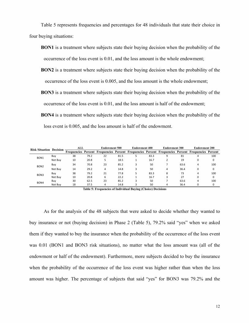
Table 5 represents frequencies and percentages for 48 individuals that state their choice in

four buying situations:

BON1 is a treatment where subjects state their buying decision when the probability of the

occurrence of the loss event is 0.01, and the loss amount is the whole endowment;

BON2 is a treatment where subjects state their buying decision when the probability of the

occurrence of the loss event is 0.005, and the loss amount is the whole endowment;

BON3 is a treatment where subjects state their buying decision when the probability of the

occurrence of the loss event is 0.01, and the loss amount is half of the endowment;

BON4 is a treatment where subjects state their buying decision when the probability of the

loss event is 0.005, and the loss amount is half of the endowment.

As for the analysis of the 48 subjects that were asked to decide whether they wanted to

buy insurance or not (buying decision) in Phase 2 (Table 5), 79.2% said “yes” when we asked

them if they wanted to buy the insurance when the probability of the occurrence of the loss event

was 0.01 (BON1 and BON3 risk situations), no matter what the loss amount was (all of the

endowment or half of the endowment). Furthermore, more subjects decided to buy the insurance

when the probability of the occurrence of the loss event was higher rather than when the loss

amount was higher. The percentage of subjects that said “yes” for BON3 was 79.2% and the

Frequencies Percent Frequencies Percent Frequencies Percent Frequencies Percent Frequencies PercentBuy 38 79.2 22 81.5 5 83.3 9 81 4 100Not1Buy 10 20.8 5 18.5 1 16.7 2 19 0 0Buy 34 70.8 23 85.2 3 50 7 63.6 4 100Not1Buy 14 29.2 4 14.8 3 50 4 36.4 0 0Buy 38 79.2 21 77.8 5 83.3 8 73 4 100Not1Buy 10 20.8 6 22.2 1 16.7 3 27 0 0Buy 30 62.5 23 85.2 3 50 7 63.6 4 100Not1Buy 18 37.5 4 14.8 3 50 4 36.4 0 0

Table 5: Frequencies of Individual Buying (Choice) Decisions

BON1

BON2

BON3

BON4

ALL Endowment 400 Endowment 300 Endowment 200Risk Situation Decision Endowment 500

13

percentage of subjects that said “yes” for BON2 was 70.8%, given that expected losses remained

the same. Given the potential amounts lost remaining the same, a higher percentage of subjects

wanted to buy insurance against BON1 (the risk situation with the probability of loss being 0.01,

and the loss amount being all of the endowment) than BON2 (the risk situation with the

probability of loss being 0.005, and the loss amount being all of the endowment) and similarly

more subjects wanted to buy BON3 (the risk situation with the probability of loss being 0.01, and

the loss amount being half of the endowment) than BON4 (the risk situation with the probability

of loss being 0.005, and the loss amount being half of the endowment). In sum, the frequency of

the buying decisions indicates that the probability of loss rather than the loss amount most

influenced subjects’ buying decisions. This conclusion, however, needs support from further

statistical analyses.

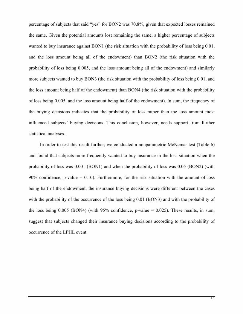
In order to test this result further, we conducted a nonparametric McNemar test (Table 6)

and found that subjects more frequently wanted to buy insurance in the loss situation when the

probability of loss was 0.001 (BON1) and when the probability of loss was 0.05 (BON2) (with

90% confidence, p-value = 0.10). Furthermore, for the risk situation with the amount of loss

being half of the endowment, the insurance buying decisions were different between the cases

with the probability of the occurrence of the loss being 0.01 (BON3) and with the probability of

the loss being 0.005 (BON4) (with 95% confidence, p-value = 0.025). These results, in sum,

suggest that subjects changed their insurance buying decisions according to the probability of

occurrence of the LPHL event.

14

The individual risk attitudes were calculated by taking the ratios of the WTP values to their

expected values (WTP/EV). A WTP/EV greater than 1 indicates risk aversion, equal to 1

indicates risk neutrality and smaller than 1 indicates a risk seeking attitude (see McClelland et

al., 1993 for further details on calculations). Accordingly, when each individual’s WTP/EV ratio

was calculated, we found that all subjects were risk averse, thus they all have WTP/EV ratios

greater than 1, which is consistent with well-known fourfold patterns of risk attitudes as

suggested by Prospect Theory (Kahneman and Tversky, 1979; Tversky and Kahneman, 1992;

Harbaugh, Krause, and Vesterlund, 2002). Intuitively, a risk averse individual would have been

more likely to state a threshold probability that is not much higher than the probabilities used to

calculate the expected values: 0.01 and 0.005. However, the mean values for the threshold

probabilities were found to be 9%, 3.7%, 5.5%, and 4.5% to buy insurance in the four loss

situations, BON1 to BON4, respectively, used in our experiment. These subjects stated way

higher threshold probabilities and thus, unfortunately, were not adequate for reasonable

interpretation.

In addition to the analyses explained above, we examined the effects of endowment,

gender, age, income, and threshold probability on individuals’ paying decisions and on their

buying decisions. We decided to use the risk situation with a probability of loss equal to 0.01 and

loss amount of all the endowment (WTP1) because it had been the most frequently used

Endowment BON1-BON2 BON1-BON3 BON2-BON4 BON1-BON4 BON2-BON3 BON3-BON4ALL 0.10 1.00 0.50 0.025 1.00 0.025500 0.10 1.00 0.50 0.025 1.00 0.025400 0.50 1.00 1.00 0.50 0.50 0.50300 0.50 1.00 1.00 0.50 1.00 0.50200

p"valuesFOR ALL CASES SUBJECTS BOUGTH, SO WE CANNOT CONDUCT THE TEST

Table 6: McNemar Test between Each Pair of Buying (Choice Decision)

15

probability and loss amount values in LPHL contexts (e.g., McClelland et al., 1993; Ganderton et

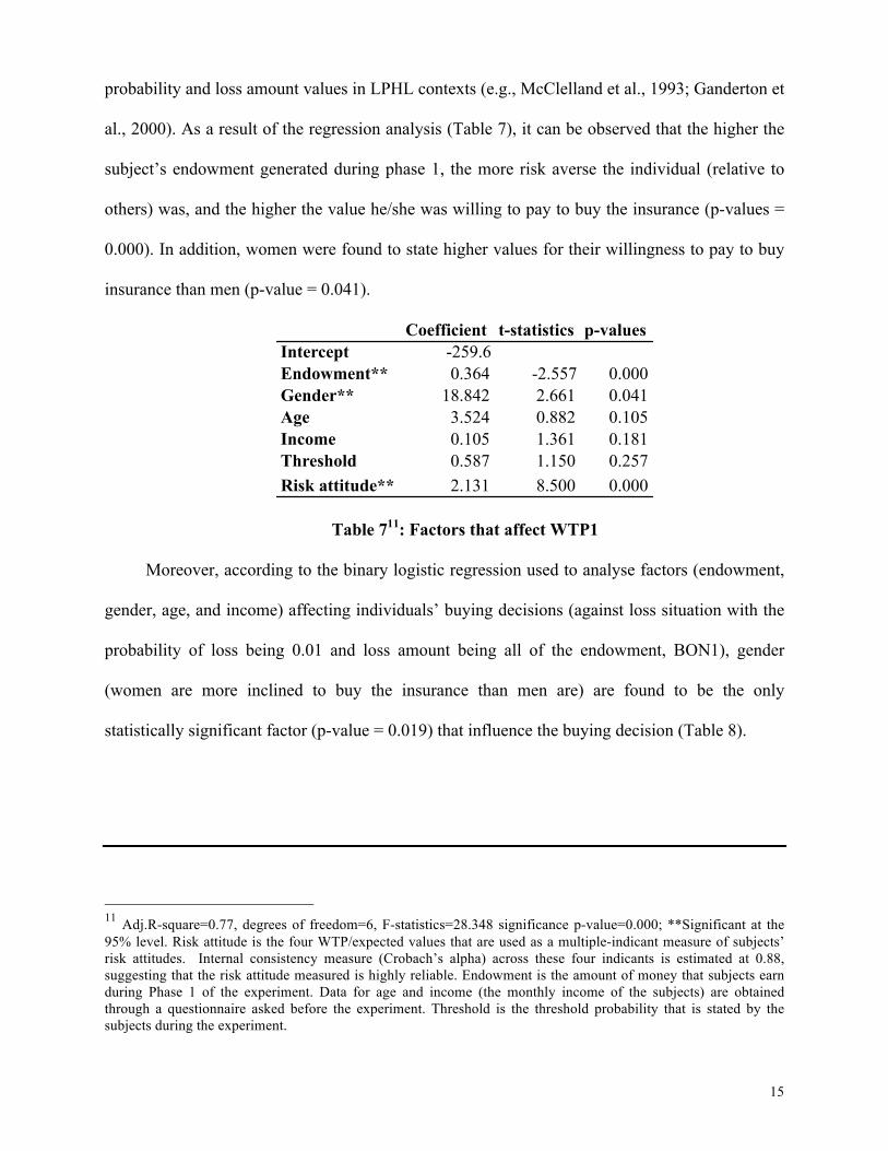
al., 2000). As a result of the regression analysis (Table 7), it can be observed that the higher the

subject’s endowment generated during phase 1, the more risk averse the individual (relative to

others) was, and the higher the value he/she was willing to pay to buy the insurance (p-values =

0.000). In addition, women were found to state higher values for their willingness to pay to buy

insurance than men (p-value = 0.041).

Table 711: Factors that affect WTP1

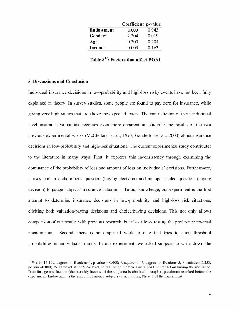
Moreover, according to the binary logistic regression used to analyse factors (endowment,

gender, age, and income) affecting individuals’ buying decisions (against loss situation with the

probability of loss being 0.01 and loss amount being all of the endowment, BON1), gender

(women are more inclined to buy the insurance than men are) are found to be the only

statistically significant factor (p-value = 0.019) that influence the buying decision (Table 8).

11 Adj.R-square=0.77, degrees of freedom=6, F-statistics=28.348 significance p-value=0.000; **Significant at the 95% level. Risk attitude is the four WTP/expected values that are used as a multiple-indicant measure of subjects’ risk attitudes. Internal consistency measure (Crobach’s alpha) across these four indicants is estimated at 0.88, suggesting that the risk attitude measured is highly reliable. Endowment is the amount of money that subjects earn during Phase 1 of the experiment. Data for age and income (the monthly income of the subjects) are obtained through a questionnaire asked before the experiment. Threshold is the threshold probability that is stated by the subjects during the experiment.

Coefficient t-statistics p-valuesIntercept -259.6Endowment** 0.364 -2.557 0.000Gender** 18.842 2.661 0.041Age 3.524 0.882 0.105Income 0.105 1.361 0.181Threshold 0.587 1.150 0.257Risk attitude** 2.131 8.500 0.000

16

Table 812: Factors that affect BON1

5. Discussions and Conclusion

Individual insurance decisions in low-probability and high-loss risky events have not been fully

explained in theory. In survey studies, some people are found to pay zero for insurance, while

giving very high values that are above the expected losses. The contradiction of these individual

level insurance valuations becomes even more apparent on studying the results of the two

previous experimental works (McClelland et al., 1993; Ganderton et al., 2000) about insurance

decisions in low-probability and high-loss situations. The current experimental study contributes

to the literature in many ways. First, it explores this inconsistency through examining the

dominance of the probability of loss and amount of loss on individuals’ decisions. Furthermore,

it uses both a dichotomous question (buying decision) and an open-ended question (paying

decision) to gauge subjects’ insurance valuations. To our knowledge, our experiment is the first

attempt to determine insurance decisions in low-probability and high-loss risk situations,

eliciting both valuation/paying decisions and choice/buying decisions. This not only allows

comparison of our results with previous research, but also allows testing the preference reversal

phenomenon. Second, there is no empirical work to date that tries to elicit threshold

probabilities in individuals’ minds. In our experiment, we asked subjects to write down the

12 Wald= 14.109, degrees of freedom=1, p-value = 0.000; R-square=0.46, degrees of freedom=5, F-statistics=7.258, p-value=0.000; *Significant at the 95% level, in that being women have a positive impact on buying the insurance. Date for age and income (the monthly income of the subjects) is obtained through a questionnaire asked before the experiment. Endowment is the amount of money subjects earned during Phase 1 of the experiment.

Coefficient p-valueEndowment 0.000 0.943Gender* 2.304 0.019Age 0.300 0.204Income 0.003 0.163

17

likelihood of the monetary loss that would make them consider buying insurance. The

experimental design also allowed us to determine individuals’ risk attitudes, which further

enabled us to see the effects of these threshold probabilities, risk attitudes, and some

demographic characteristics of subjects (such as income, gender, and age) on their buying and

paying insurance decisions.

Our results showed that when individuals were asked to state their willingness-to-pay for

insurance (paying decision), they perceived the risk to be higher in the case of a higher amount

of loss rather than a higher probability of loss. However, when individuals were asked whether

they would buy the insurance or not (buying decision), the outcome of the buy or not responses

supported the probability of loss rather than the loss amount on the individual’s decision making.

This finding supports Ganderton’s et al. (2000) conclusion. They also used buy or not questions

(rather than willingness to pay questions) when they stated the relative importance of probability

on individual insurance buying decisions.

In summation, an important contribution of this study is revealing the distinction between

the buying (choice) decision and the paying (valuation/pricing) decision embodied in the

different descriptions of willingness to reduce low-probability and high-loss risk. This result

seems supportive of the preference reversal phenomenon (individuals may consider different

kinds of information when they make choice versus pricing decisions) of which the significance

remains even in experiments with different structures (Pommerehne et al., 1982). In fact,

“regulatory agencies even distinguish between probabilistic (concerned with likelihood) and

deterministic (concerned with magnitude) risk assessments” (Kuhn and Budescu, 1996).

However, economic theory does not distinguish the risk reduction measures along these lines.

When people decide whether to buy insurance or not against events, they focus on lower

probability, thus, intention to buy without any concern about price of insurance is affected by the

18

probability of loss. This may be a possible reason why people do not prefer to insure themselves

against low-probability, high-loss events (e.g., natural disasters and bankruptcy). However, when

people pass the intention stage and decide to buy, they primarily take into account the high loss

amount for pricing insurance. Hence, once insurance companies convince individuals to buy

insurance by explaining the effectiveness or usefulness of insurance itself, rather than focusing

on the risk (because people take into account low probability of loss rather than high loss amount

and thus do not really worry about risk), they can persuade people to pay high amounts of money

to buy insurance (because people focus on high loss amount when making paying decisions). In

addition, all subjects were found to be risk averse, which is consistent with well-known fourfold

patterns of risk attitudes as suggested by Prospect Theory: risk averse for gains and risk seeking

for losses in high probability events, and risk averse for losses and risk seeking for gains in low

probability events. The threshold probabilities, on average, are much higher than the

probabilities used to calculate the expected values and seem to have no significant correlation

with any variable, providing no support for the prospective reference theory. In fact, the results

of the regression analysis indicate that threshold probability was an insignificant factor in

insurance valuations for both paying and buying decisions. The analysis also showed that

individuals’ initial endowment had a positive impact on the value of their willingness to pay.

Finally, it is important to note that being female had a positive impact on, both, individual

insurance buying decisions and paying decisions. This finding offers guidelines for businesses in

the insurance industry in motivating low-probability and high-loss risk mitigation.

The current study suggests that the inconsistent findings in prior research may be due to

differences in elicitation methods. For example, the studies that use dichotomous questions to

ask individuals’ insurance purchase decisions mostly found the probability of loss most

19

influenced the decision (e.g., Ganderton et al., 2000), which does not support the findings of

McClelland’s et al. (1993) study, which uses open-ended willingness to pay questions. For

further studies, insurance can be assumed to reduce the possible monetary loss to a certain level

rather than to zero. Various elicitation mechanisms (see Holt, 1986 for the drawbacks of paying

only one round) and loss situations with different probabilities and loss amounts could be used to

investigate the distinction between insurance payments and choice decisions to generalise the

results. The dichotomous versus open-ended questions approach used to elicit individual

protection valuation can be designed to enable the researcher to compare both risk attitude

measurements. The current experiment takes the expected values as the prices of the insurances

in order to gauge individuals’ self-determined threshold probabilities and different price levels

may contribute further information. Finally, an extended theoretical investigation is necessary to

support the findings of the current experiment’s results.

References

Arrow, K. J. (1996), “The theory of risk bearing: small and great risks,” Journal of Risk and Uncertainty 12(2/3), 103-111. Becker, G. M., M. E. De Groot, and J. Marschak, (1964), “Measuring utility by a single response sequential method,” Behavioral Science 9, 226-232. Borling, A., Hans Keiding (2002), “Stochastic dominance and conditional expectation-an insurance theoretical approach,” The Geneva Papers on Risk and Insurance Theory 27, 31-48. Brookshire, D. S., M. A. Thayer, J. Tschirhart - W. D. Schulze (1985), “A test of the expected utility model: evidence from earthquake risks,” Journal of Political Economy 93(2), 369-389. Camacho-Cuena, E., C. Seidl, A. Morone, (2005), “Comparing preference reversal for general lotteries and income distributions” Journal of Economic Psychology, vol. 26 (5), 682-710.

Camerer, C. F., H. Kunreuther (1989), “Decision processes for low probability events: policy implications,” Journal of Policy Analysis and Management 8(4), 565-592.

20

Camerer, C. (1995), Individual Decision Making, in J. H. Kagel, and A. E. Roth, Handbook of Experimental Economics, Princeton University Press, 587-616. Cook, P. J., D. A. Graham (1975), The Demand for Insurance and Protection: The Case of the Irreplaceable Commodity. Draft Report, Duke University, North Carolina. Di Mauro, C., and Maffioletti A. (2004), “Attitudes to risk and attitudes to uncertainty: Experimental evidence,” Applied Economics, 36, 357-72. Dong, W., H. C. Shah, F. Wong (1996), “A rational approach to pricing of catastrophe insurance,” Journal of Risk and Uncertainty 12(2/3), 201-219. Drehmann, M., J. Oechssler, A. Roider (2007), „Herding with and without payoff externalities-an internet experiment,” International Journal of Industrial Organization 25, 391-415. Etchart-Vincent, N. (2004), “Is probability weighting sensitive to the magnitude of consequences: an experimental investigation on losses,” Journal of Risk and Uncertainty 28 (3), 217-235. Fischbacher, U. (2007), “Zurich toolbox for readymade economic experiments,” Experimental Economics, 10, 171-178. Ganderton, P. T., D. S. Brookshire, M. McKee, S. Steward, H. Thurston (2000), “Buyinginsurance for disaster-type risks: experimental evidence,” Journal of Risk and Uncertainty 20 (3), 271-289. Greiner, B. (2004), An Online Recruitment System for Economic Experiments. In: Kremer, K., Macho, V. (Eds.). Grether, D.M. Plott, C. R. (1979), “Economic theory of choice and the preference reversal phenomenon,” American Economic Review 69 (4), 623-638. Harbaugh, W., K. Krause, L. Vesterlund, 2002. Prospect theory in choice and pricing tasks,” University of Oregon, Economics Department, Working papers, 27. Hershey, J. C. P. J.H. Schoemaker (1980), “Risk taking and problem context in the domain of losses: an expected utility analysis,” Journal of Risk and Insurance 47 (1), 111-132. Hey, J.D., J. Lee (2005), “Do subjects separate (or are they sophisticated)?,” Experimental Economics 8, 233-265. Hey, J.D., Morone, A., Schmidt, U., (2009) “Noise and Bias in Eliciting Preferences”, Journal of Risk and Uncertainty, vol. 39(3): 213-235.

Holt, C.A. (1986), “Preference reversals and the independence axiom,” American Economic Review 76 (3), 508-515. Kagel, J. H., A. E. Roth (1995), The Handbook of Experimental Economics, Princeton.

21

Kahneman, D., A. Tversky (1979), “Prospect theory, an analysis of decision under risk,” Econometrica 47, 263-291. Kuhn, K. M., Budescu D. V. (1996), “The relative importance of probabilities, outcomes, and vagueness in hazard risk decisions,” Organizational Behavior and Human Decision Processes 68 (3), 301-317. Kunreuther, H., P. Slovic (1978), “Economics, psychology, and protective behavior,” American Economic Review 68:2, Papers and Proceedings of the Ninetieth annual Meeting of the American Economic Association, 64-69. Laury, S. K. (2006), Pay one or pay all: random selection of one choice for payment. http://expecon.gsu.edu/workingpapers/GSU_EXCEN_working_paper_2006-24.pdf Machina, M.J., Pratt, J.W. (1997), “Increasing risk: some direct constructions,” Journal of Risk and Uncertainty 14, 103-127. McClelland, G. H., W. D. Schulze, B. Hurd (1990), “The effect of risk beliefs on property values: a case study of a hazardous waste site,” Risk Analysis 10(4), 485-97. McClelland, G. H., W. D. Schulze, D. L. Coursey (1993), “Insurance for low-probability hazards: a bimodal response to unlikely events,” Journal of Risk and Uncertainty 7, 95-116. McDaniels, T. L., M. S. Kamlet, G. W. Fischer (1992), “Risk perception and the value of safety,” Risk Analysis 12 (4), 495-503. Meroz, Y., Morone A. ,Morone P., (2012) “Eliciting environmental preferences of Ghanaians in the laboratory: An incentive compatible experiment” International Journal of Environment and Sustainable Development

Morgenstern, O. (1979), Some Reflections on Utility Theory, the Expected Utility Hypothesis and the Allais Paradox, M. Allais and O. Hagen, eds., Dorbrecht: D. Reidel. Morone, A., U. Schmidt, (2008) “An Experimental Investigation of Alternatives to Expected Utility Using Pricing Data”, Economics Bulletin, vol. 4(20): 1-12. Morone, A., (2008) “Comparison of Mean-Variance Theory and Expected-Utility Theory through a Laboratory Experiment”, Economics Bulletin, vol. 3(40), pages 1-7. Morone, A., (2010), “On price data elicitation: A laboratory investigation” The Journal of Socio-Economics, vol. 39(5): 540-545

22

Morone, A., Ozdemir O., (2012) “Displaying Uncertain information About Probability: Experimental Evidence” Bulletin of Economic Research, 2012. Morone, A., P. Morone, (2012), "Are small groups expected utility?," MPRA Paper 38198, University Library of Munich, Germany.

Müller, A. (1998), “Comparing risks with unbounded distributions,” Journal of Mathematical Economics 30, 229-239. Plott, C. R., Zeiler K.(2005), „The willingness to pay- willingness to accept gap, the “endownment effect”, subject misconceptions, and experimental procedures for eliciting valuations,” American Economic Review 95 (3), 530-45. Pommerehne, W.W., F., Schneider, P. Grether, C.R. Plott (1982), “Economic theory of choice and the preference reversal phenomenon: a reexamination/reply,” American Economic Review 72 (3), 569-576. Rothschild, M., Stiglitz, J.E.(1970), “Increasing risk: I. A. definition,” Journal of Economic Theory 2, 225-243. Segal, U. (1988), “Does the preference reversal phenomenon necessarily contradict the independence axiom?,” American Economic Review 78 (1), 233-236. Sjöberg, L. (1999), “Consequences of perceived risk: Demand for mitigation,” Journal of Risk Research 2, no.2: 129-149. Slovic, P., B. Fischhoff, S. Lichtenstein, B. Corrigan, B. Combs (1977), “Preference for insuring against probable small losses: insurance implications,” Journal of Risk and Insurance 44(2), 237-258. Slovic, P., B. Fischhoff, S. Lichtenstein (1980), Facts and fears: Understanding perceived risk. Societal risk assessments: how safe is safe enough? Edited by Richard C. Schwing and Walter Albers, Jr. Plenum Press, New York. Starmer, C., R. Sugden (1991), “Does the random-lottery incentive system elicit true preferences? An experimental investigation,” American Economic Review 81(4), 971-78. Thaler, R.H., Johnson E.J. (1999), “Gambling with the house money and trying to break even: the effects of prior outcomes on risky choice,” Management Science 36 (6), 643-60. Traub, S., C. Seidl, A. Morone, (2006), “Relative Deprivation, Personal Income Satisfaction, and Average Well-Being under Different Income Distributions” in M. McGillivray (ed.), Inequality, Poverty and Human Well-being, Palgrave, 2006.

23

Tversky, A., P. Slovic, and D. Kahneman (1990), “The Causes of Preference Reversal,” American Economic Review, 80, 204-217. Tversky, A., S. Sattath, and P. Slovic (1988), “Contingent weighting in judgment and choice,” Psychological Review 95: 371-84. Tversky, A., Kahneman D. (1981), “The framing of decisions and the psychology of choice,” Science 221,453-458. Viscusi, W. K., W. N. Evans (1990), “Utility functions that depend on health status: estimates and economic implications,” American Economic Review 80 (3), 353-74.