


![DETRENDED TOPOGRAPHIC DATA OF THE SOUTH … · surface, detailing the interior composition [3, 4], ... Conclusions: Detrended topographic data provide a quantifiable method for enhancing](https://static.fdocuments.in/doc/165x107/5adb1d647f8b9a6d318dabfc/detrended-topographic-data-of-the-south-detailing-the-interior-composition-3.jpg)
Languages
Pages
Legal

Multifractal Detrended Fluctuation Analysis ofInsole Pressure Sensor Data to Diagnose VestibularSystem DisordersBatuhan Günaydın
Istanbul Technical UniversitySerhat İkizoğlu ( [email protected] )
Istanbul Technical University
Research Article
Keywords: Vestibular disorders, non-stationary time series, multi-fractality, detrending, long-rangecorrelations, classi�cation
Posted Date: September 30th, 2021
DOI: https://doi.org/10.21203/rs.3.rs-934139/v1
License: This work is licensed under a Creative Commons Attribution 4.0 International License. Read Full License
1
Multifractal Detrended Fluctuation Analysis of
Insole Pressure Sensor Data to Diagnose Vestibular
System Disorders
Batuhan Günaydın1, Serhat İkizoğlu1 1Department of Control and Automation Engineering, Faculty of Electric and Electronics, Istanbul Technical University (ITU), Istanbul, Turkey
Corresponding author: Serhat İkizoğlu, Address: ITU Electric-Electronics Faculty, Control and Automation Eng. Dept., 34469 Maslak-Istanbul, Turkey; e-mail: [email protected]
Abstract – The vestibular system (VS) is a sensory system that has a vital function in human life
by serving to maintain balance. In this study, multifractal detrended fluctuation analysis (MFDFA)
is applied to insole pressure sensor data collected from subjects in order to extract features to
identify diseases related to VS dysfunction. We use the multifractal spectrum width as the feature
to distinguish between healthy and diseased people. It is observed that multifractal behavior is more
dominant and thus the spectrum is wider for healthy subjects, where we explain the reason as the
long-range correlations of the small and large fluctuations of the time series for this group. We
directly process the instantaneous pressure values to extract features in contrast to studies in the
literature where gait analysis is based on investigation of gait dynamics (stride time, stance time,
etc.) requiring long gait cycles. Thus, as the main innovation of this work, we detrend the data to
give meaningful information even for a relatively short-duration gait cycle. Extracted feature set
was input to fundamental classification algorithms where the Support-Vector-Machine (SVM)
performed best with an accuracy of 98.2% for the binary classification as healthy or suffering. This
study is a substantial part of a big project where we finally aim to identify the specific VS disease
that causes balance disorder and also determine the stage of the disease, if any. Within this scope,
the achieved performance gives high motivation to work more deeply on the issue.
Keywords – Vestibular disorders, non-stationary time series, multi-fractality, detrending, long-
range correlations, classification.
-------------------------------------------------------
Batuhan Günaydın (present address): Calibration Engineer at AVL Research & Engineering TR,
Abdurrahmangazi Mah., Atatürk Cad. No: 22 /11-12, 34885 Istanbul- Turkey.
2
1. INTRODUCTION
The vestibular system is a perceptual system with the mission of providing intel to our brain about spatial
orientation, head position and motion. Besides, it is also filled with motor functions to preserve balance, to
counterbalance head and body while we move and to keep our posture stable [1]. Even though there are numerous
studies about a number of issues in various branches in the medical field, it is hard to consider detection of
vestibular disorders among the prominent areas of interest. The lack of studies in such a crucial field of medicine
is the main motivation of this study.
To analyze and diagnose balance disorders, various methods have been experimented on different types of data.
Among those, human gait dynamics are frequently used to diagnose neurodegenerative diseases (NDDs) such as
Parkinson disease (PD), Huntington disease (HD) and amyotrophic lateral sclerosis (ALS). As an example, to
diagnose PD, Abdulhay et al. worked on gait dynamics. They filtered the force data and applied peak detection
and pulse duration measuring techniques to extract features such as stride time, stance time, swing time and foot
strike profile [2]. Daliri also used these features and added double support interval to extract even more features.
He then applied genetic algorithms to select appropriate features and classified NDDs with the obtained feature
set [3]. Sarbaz et al. exploited the semi periodic structure of human gait and its fractal properties to model PD and
healthy gait dynamics with sine-circle map method. They managed to distinct two patterns with the model
parameter “Ω” [4]. Zeng and Wong used radial basis function neural networks to obtain gait patterns and
performed classifications with various estimators making use of deterministic learning to diagnose NDDs [5].
We observe that studies on detecting VS dysfunctions causing balance disorder are not carried out as intensively
as they are concentrated on NDDs. In this area, the well-known computerized dynamic posturography (CDP) is
still the most widely used technique; however, alternative methods are spreading fast in recent years. Studies in
the literature do not only concentrate on the gait analysis, but we also meet different approaches. In this context,
Imai et al. analyzed eye rotation vectors of samples to diagnose benign paroxysmal positional vertigo (BPPV) [6].
Lang et al performed 3D motion analysis to evaluate locomotor pattern and body's oscillation during gait under
different conditions in VS patients [7]. Bergeron et al analyzed the effect of virtual reality tools on detection of
VS disorders from different aspects [8]. Sang-I et al measured the balance performance when responding to visual
stimuli in subjects with BPPV [9]. Auvinet et al applied dual task gait analysis to detect gait disorders related to
several diseases including VS-based in the elderly people [10].
In our study we decided to extract features related to gait. The main reason behind this decision was that we aimed
for wearable sensors to ensure that patients do not have to be tested in a clinical setting and are tracked in their
daily lives. Besides, respected academicians in the field of audiology also encouraged us to follow the way we
started as there are not sufficient studies conducted using the method we considered on VS disorder detection. In
the literature, gait analysis is carried out mainly based on three approaches. These are: Image processing, where
gait will be analyzed by processing the camera records; using force sensors, either placed under the sole of the
3
subject or by utilizing floor sensors; making use of inertial/motion sensors, placed on appropriate points on the
body [11, 12, 13]. The collected data will then be used to extract features based on both the frequency and time
domain analysis such as step length, step width, speed, foot ascension from ground etc. [14]. Within this frame,
Jarchi et al presented a review on accelerometry based gait analysis [15]. Ricciardi et al applied different machine
learning algorithms to classify Parkinsonism using gait analysis’ parameters where they used 16 features [16].
Sama et al. analyzed the body sensor data to find spatio-temporal properties of human gait [17]. Zhao et al.
developed a dual channel LSTM based multi-feature extraction method for gait analysis [18]. Tao et al reviewed
available wearable sensors and ambulatory gait analysis methods based on various wearable sensors [19].
In fact, the experimental setup and the raw data collected in many of the studies about gait analysis using insole
pressure sensors are quite similar with our work. However, as a novelty brought in our study, we used
instantaneous pressure data to extract features directly rather than to use these data to calculate specific time
intervals (such as stride time, stance time, swing time etc.) associated with the gait. We analyzed the changes in
the pressure values on each insole sensor to extract information about the change in the behavior of giving strength
on different parts of the foot during walking.
Regarding the feature extraction method, fractal/multifractal time series analysis, MFDFA and detrended
fluctuation analysis (DFA) have been applied on different fields/cases in the literature such as EEG, stock market,
wind speed, heart rate dynamics, precipitation amount, medical images, traffic, human gait etc. [20-27]. Common
characteristic of all these signals/data is that they either have fluctuations on a wide range of time scales or their
values show broad distributions so that their behavior will be described with a power law. As an application of
the fractal time series analysis on gait data, Hausdorff et al. illustrated that human walking and random walking
demonstrate severe correlations [28]. They claimed that healthy people have a more compact time series compared
to diseased people and they also observed a similar discrepancy between young and elder individuals, which was
later also supported by the study of Diosdado et al [29]. Kirschner et al. applied DFA and adaptive fractal analysis
(AFA) on human gait. To overcome the problem with short term data, they merged 5 walking sets with each
consisting of 25 strides [30]. Dutta et al. used MFDFA to analyze stride intervals of control, HD and PD groups.
They showed that there is a big difference in spectrum widths of diseased and healthy people [27].
In the whole of our project about identifying the specific disease behind the balance disorder sourcing from VS
problems, we investigate the contributions of features extracted from data collected by both the inertial and force
sensors and we also perform analysis both in frequency and time domain [14, 31, 32, 33]. The main reason behind
the choice of time series analysis method and specifically the multifractal analysis in this study is the fact that gait
data present multifractal scaling behavior as mentioned above. A careful literature research puts forth that
although human gait appears to have regular dynamics, it actually incorporates small and large fluctuations which
are long range correlated in healthy case [27-29]. In our study, this feature is expected to provide useful
information to capture important features to be used for classification. On the other hand, to extract useful
4
information from individual samples, in other words, to reveal small fluctuations, we need to detrend the data.
Therefore, among multifractal analysis we decided on MFDFA as the method to apply.
To summarize the contributions of our work: Quantitatively, studies to determine the diseases based on VS
dysfunction are insufficient in the literature. Additionally, almost all studies have focused on similar features of
gait analysis that require long gait cycles. This study searches for new features to identify VS related diseases
where we aim to increase the accuracy in the detection and also shorten the data acquisition period. In this context,
MFDFA has been applied to instantaneous pressure-sensor data collected from wearable insole sensors. This also
allows data to be obtained in daily life that helps the patient to escape the stress of the clinical environment and
thus avoids adverse effect of the process on the accuracy of the diagnosis.
After feature extraction by applying the MFDFA, a model was trained by the feature set using various
classification methods such as SVM, Decision Tree (DT), k-Nearest Neighbor (KNN) etc. To describe the content
and flow of the work clearly, the rest of this article is arranged as follows: In Section 2 the MFDFA is described
briefly. This section also provides detailed information about the data acquisition process. In Section 3 we submit
and discuss the numerical results of the experiments conducted. Finally, we draw conclusions from the study and
mention about the future work regarding the use of the outcomes of this study in the whole project.
2. MATERIALS & METHOD
2.1 APPLIED METHOD: THE MFDFA
Briefly, MFDFA consists of five steps. At the first step, the profile of the time series is calculated by subtracting
the mean value from each sample and taking the cumulative sum of the samples. As the second step, the new time
series or the so-called profile is divided into non-overlapping segments of equal lengths. Next, each segment gets
least square fitted and corresponding values of the regression curve are subtracted from the individual values
within the segment. Following this step, the variance of each segment is calculated. As the fourth step, qth order
fluctuation function is calculated for each segment. The steps two to four are repeated for different q and s
(segment size) values. At the final step, log-log plots of the qth order fluctuation function and segment sizes are
analyzed; scaling exponent and singularity strength are calculated and the multi-fractal spectrum is drawn. The
width of the spectrum demonstrates the amount of multi-fractality of the time series.
Below we summarize the mathematics behind this method which was developed by Kantelhardt et al. in 2002
[34].
Step 1: Determining the profile
Let us suppose a time series x(i) with i = 1…N (N: length of the series). Now, the profile is obtained as
5
𝑌(𝑖) = ∑[𝑥(𝑘) − 𝑥𝑎𝑣] for 𝑖 = 1 … 𝑁 𝑖𝑘=1 (1)
where 𝑥𝑎𝑣 is the mean of the time series.
Step 2: Dividing the profile into segments
The profile Y(i) of the length N is divided into Ns non- overlapping segments which are all equally sized with s.
But since in general N will not be an integer multiple of s, the procedure about the division of the time series into
segments will also be run backward in order to cover all samples; this is, starting with the last sample of the series
and propagate backward toward the first one. Thus, we finally have 2Ns segments, each of the size s.
Step 3: Detrending and Variance Calculation
As the next step, the variance of each segment is calculated. The variance is a measure of the power of the tendency
to deviate from the mean. For dynamic systems, where we cannot refer to a constant mean value, we are interested
in the deviation from the trend, so we need to determine the trend within the segment in order to speak about a
meaningful deviation. The trend is determined and a regression curve is obtained by least square fitting and then
for each sample, the value on this curve will be subtracted from the corresponding sample value within the
segment. This process is called detrending. The variance will then be calculated as
𝐹2(𝑣, 𝑠) = 1𝑠 ∑{𝑌[(𝑣 − 1)𝑠 + 𝑖]𝑠𝑖=1 − 𝑦𝑣(𝑖)}2 (2)
for 𝑣 = 1, …, Ns and
𝐹2(𝑣, 𝑠) = 1𝑠 ∑{𝑌[𝑁 − (𝑣 − 𝑁𝑠)𝑠 + 𝑖]𝑠𝑖=1 − 𝑦𝑣(𝑖)}2 (3)
for 𝑣 = Ns+1, …, 2Ns.
In these equations 𝑦𝑣(𝑖) is the least square fitted polynomial for each segment 𝑣. The choice of the degree m of
the polynomial is optional and case dependent; in our case we chose m=2, since the profiles were illustrating
piecewise near-parabolic behaviours. We also performed calculations for m=3 to verify our foresight and obtained
similar results as for m=2.
Step 4: Calculating the fluctuation function
Multi-fractality in time series is an indicator of the existence of small and large fluctuations in contrast to mono-
fractal time series, where 2nd order statistical moments give sufficient information about the series. Thus, for the
multifractal case, qth order statistical moments have to be considered where q is not limited with 2 [35].

6
𝐹𝑞(𝑠) = { 12𝑁𝑠 ∑[𝐹2(𝑣, 𝑠)]𝑞22𝑁𝑠𝑣=1 }1𝑞 (4)
Here, q can take any real value; for q →0, Eq. 5 is used since 1/q in Eq. 4 approaches to infinity for this condition
[27].
𝐹0(𝑠) = 𝑒𝑥𝑝 { 14𝑁𝑠 ∑ 𝑙𝑛 [𝐹2(𝑣, 𝑠)]2𝑁𝑠𝑣=1 } ~ 𝑠ℎ(0) (5)
where h(q) is the so-called Hurst exponent.
Step 5: This process is repeated for various s and q values, so that the relationship between Fq(s) and h(q) is
illustrated on log-log plot. If the series is long range correlated, we observe a power law behaviour as [27] 𝐹𝑞(𝑠)~𝑠ℎ(𝑞) It is obvious that if this scaling exists, ln(Fq(s)) will linearly depend on ln(s) with the slope of generalized Hurst
exponent h(q). Generally, for monofractal time series h(q) is identical for all q values; in other words, the
logarithmic relationship between Fq(s) and s is not dependant on q for monofractal time series [36]. Since
multifractal series cannot be expressed by a unique h(q), a spectrum of generalized Hurst exponents is required to
interpret the multifractality of time series.
In order to obtain the spectrum of generalized Hurst exponents or the so-called multifractal spectrum, we go the
following steps:
First, h(q) is related to the scaling exponent τ(q) via Equation 6 [28]. 𝜏(𝑞) = 𝑞ℎ(𝑞) − 1 (6)
For mono-fractal series, τ(q) depends linearly on q since h(q) is constant, whereas multifractal series illustrate
nonlinear relationship between τ(q) and q while h(q) varies.
Once the scaling exponent is found, the singularity strength α is calculated and the singularity spectrum f(α) is
defined as 𝛼 = 𝜏′(𝑞) = 𝑞ℎ′(𝑞) + ℎ(𝑞) (7) 𝑓(𝛼) = 𝑞𝛼 − 𝜏(𝑞) = 𝑞[𝛼 − ℎ(𝑞)] + 1 (8)
The multifractal spectrum width provides crucial information about the time series. The width of the spectrum
defines the range of the exponents and is calculated as 𝑊 = 𝛼𝑚𝑎𝑥 − 𝛼𝑚𝑖𝑛 (9)
7
In this study, W is taken as the feature to determine the class the subject belongs to.
2.2 DATA ACQUISITION PROCESS
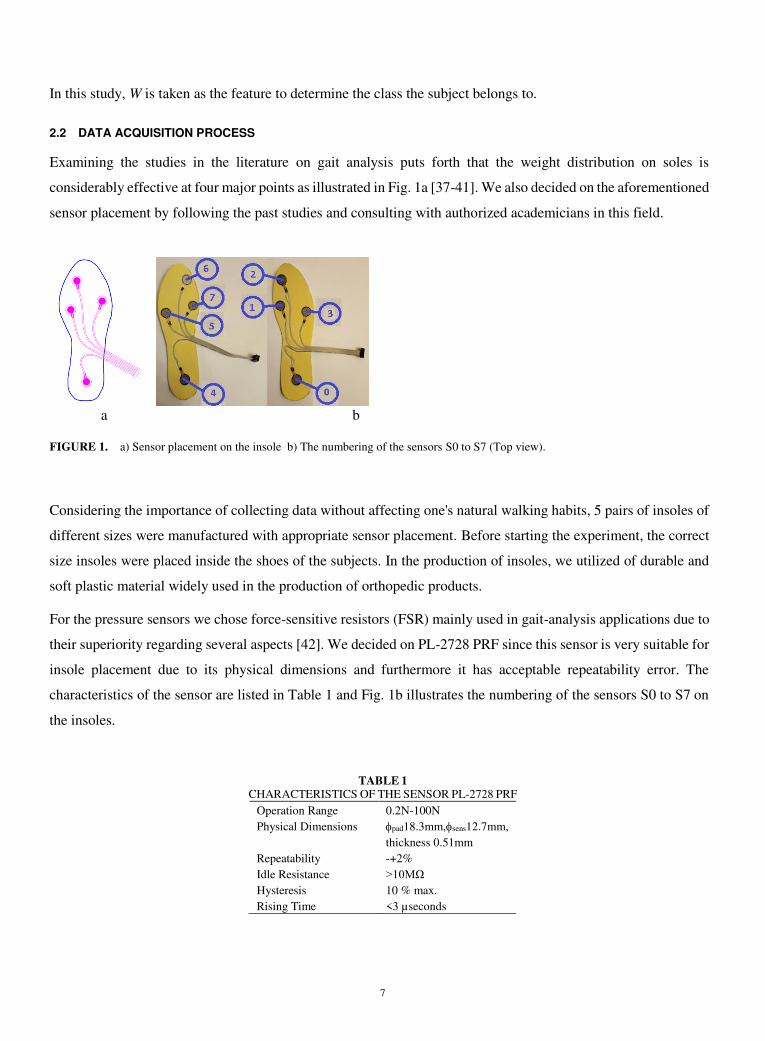
Examining the studies in the literature on gait analysis puts forth that the weight distribution on soles is
considerably effective at four major points as illustrated in Fig. 1a [37-41]. We also decided on the aforementioned
sensor placement by following the past studies and consulting with authorized academicians in this field.
a b
FIGURE 1. a) Sensor placement on the insole b) The numbering of the sensors S0 to S7 (Top view).
Considering the importance of collecting data without affecting one's natural walking habits, 5 pairs of insoles of
different sizes were manufactured with appropriate sensor placement. Before starting the experiment, the correct
size insoles were placed inside the shoes of the subjects. In the production of insoles, we utilized of durable and
soft plastic material widely used in the production of orthopedic products.
For the pressure sensors we chose force-sensitive resistors (FSR) mainly used in gait-analysis applications due to
their superiority regarding several aspects [42]. We decided on PL-2728 PRF since this sensor is very suitable for
insole placement due to its physical dimensions and furthermore it has acceptable repeatability error. The
characteristics of the sensor are listed in Table 1 and Fig. 1b illustrates the numbering of the sensors S0 to S7 on
the insoles.
TABLE 1 CHARACTERISTICS OF THE SENSOR PL-2728 PRF
Operation Range
Physical Dimensions
0.2N-100N
pad18.3mm,sens12.7mm,
thickness 0.51mm
Repeatability -+2%
Idle Resistance >10MΩ
Hysteresis 10 % max.
Rising Time <3 µseconds
8
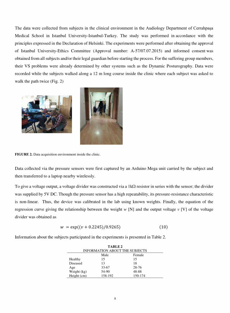
The data were collected from subjects in the clinical environment in the Audiology Department of Cerrahpaşa
Medical School in Istanbul University-Istanbul-Turkey. The study was performed in accordance with the
principles expressed in the Declaration of Helsinki. The experiments were performed after obtaining the approval
of Istanbul University-Ethics Committee (Approval number: A-57/07.07.2015) and informed consent was
obtained from all subjects and/or their legal guardian before starting the process. For the suffering group members,
their VS problems were already determined by other systems such as the Dynamic Posturography. Data were
recorded while the subjects walked along a 12 m long course inside the clinic where each subject was asked to
walk the path twice (Fig. 2)
FIGURE 2. Data acquisition environment inside the clinic.
Data collected via the pressure sensors were first captured by an Arduino Mega unit carried by the subject and
then transferred to a laptop nearby wirelessly.
To give a voltage output, a voltage divider was constructed via a 1k resistor in series with the sensor; the divider
was supplied by 5V DC. Though the pressure sensor has a high repeatability, its pressure-resistance characteristic
is non-linear. Thus, the device was calibrated in the lab using known weights. Finally, the equation of the
regression curve giving the relationship between the weight w [N] and the output voltage v [V] of the voltage
divider was obtained as 𝑤 = exp ((𝑣 + 0.2245)/0.9265) (10)
Information about the subjects participated in the experiments is presented in Table 2.
TABLE 2 INFORMATION ABOUT THE SUBJECTS
Male Female
Healthy 15 15
Diseased 13 18
Age 33-67 28-76
Weight (kg)
Height (cm)
54-90
158-192
48-88
150-174

9
The distribution of the diseases of suffering subjects is given in Table 3.
TABLE 3 THE DISTRIBUTION OF THE DISEASES OF SUFFERING SUBJECTS
Male Female
BPPV* 6 8
UVW* 3 4
Meniere 3 3
Vestibular Neuritis 1 3 *) BPPV- Benign paroxysmal positional vertigo, UVW-Unilateral vestibular weakness
The identification of all participants has been made anonymous for the publication of this paper.
3. RESULTS & DISCUSSION
In this section, the whole process is explained on a sample dataset. The captured data were first preprocessed
before features were extracted from them. At this stage, the data about the first and the last steps were removed
from the whole gait cycle data since these data are far from giving correct information; this is because the
mentioned steps do not involve in full dynamic behavior. Segment scales were set proportional to step sizes for
each subject. Hence, the segment lengths differ from subject to subject, but they are proportional to step sizes in
each case.
It is obvious that the corresponding pressure values will be around zero while the foot is in the air. The samples
taken during these intervals have to be removed from the whole dataset in order to consider the true time series
and thus avoid erroneous measurements. For this reason, precise thresholds were determined to detect that the
foot did not touch the ground.
Obviously, each subject weighs differently. On the other hand, we are interested in the deviation of the sample
values from the trend within the segment. It is necessary to handle relative deviations rather than absolute ones to
give a meaningful idea. Thus, we normalized each sensor dataset before proceeding to profiling. For the
normalization process the reference within each subject was taken as the sum of the readings of all sensors of one
foot at a moment the foot touches the ground. The assumption behind this idea is that the abovementioned
reference value is proportional to the weight of the subject.
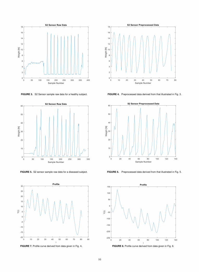
Fig. 3&4 and Fig. 5&6 illustrate sample raw and preprocessed data for healthy and diseased subjects, respectively
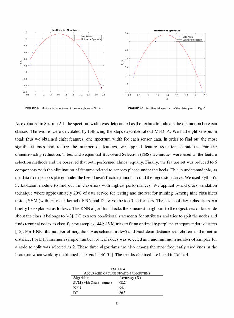
(Sensor S2). The corresponding profile curves are presented in Fig. 7&8. The multifractal spectrums for the data
and the corresponding profiles described in Section 2 are illustrated in Fig. 9&10 together with curve fittings of
2nd order polynomials.
10
FIGURE 3. S2 Sensor sample raw data for a healthy subject. FIGURE 4. Preprocessed data derived from that illustrated in Fig. 3.
FIGURE 5. S2 sensor sample raw data for a diseased subject. FIGURE 6. Preprocessed data derived from that illustrated in Fig. 5.
FIGURE 7. Profile curve derived from data given in Fig. 4. FIGURE 8. Profile curve derived from data given in Fig. 6.
11
FIGURE 9. Multifractal spectrum of the data given in Fig. 4. FIGURE 10. Multifractal spectrum of the data given in Fig. 6.
As explained in Section 2.1, the spectrum width was determined as the feature to indicate the distinction between
classes. The widths were calculated by following the steps described about MFDFA. We had eight sensors in
total; thus we obtained eight features, one spectrum width for each sensor data. In order to find out the most
significant ones and reduce the number of features, we applied feature reduction techniques. For the
dimensionality reduction, T-test and Sequential Backward Selection (SBS) techniques were used as the feature
selection methods and we observed that both performed almost equally. Finally, the feature set was reduced to 6
components with the elimination of features related to sensors placed under the heels. This is understandable, as
the data from sensors placed under the heel doesn't fluctuate much around the regression curve. We used Python’s
Scikit-Learn module to find out the classifiers with highest performances. We applied 5-fold cross validation
technique where approximately 20% of data served for testing and the rest for training. Among nine classifiers
tested, SVM (with Gaussian kernel), KNN and DT were the top 3 performers. The basics of these classifiers can
briefly be explained as follows: The KNN algorithm checks the k nearest neighbors to the object/vector to decide
about the class it belongs to [43]. DT extracts conditional statements for attributes and tries to split the nodes and
finds terminal nodes to classify new samples [44]; SVM tries to fit an optimal hyperplane to separate data clusters
[45]. For KNN, the number of neighbors was selected as k=5 and Euclidean distance was chosen as the metric
distance. For DT, minimum sample number for leaf nodes was selected as 1 and minimum number of samples for
a node to split was selected as 2. These three algorithms are also among the most frequently used ones in the
literature when working on biomedical signals [46-51]. The results obtained are listed in Table 4.
TABLE 4
ACCURACIES OF CLASSIFICATION ALGORITHMS
Algorithm Accuracy (%)
SVM (with Gauss. kernel) 98.2
KNN 94.4
DT 86.5
12
4. CONCLUSION
In this study, MFDFA was applied to insole pressure sensor data as a time-series based method to analyze human
gait to classify healthy and VS diseased people. In this context, the spectrum width was used as the feature to
distinguish between the classes. As the main contribution of this work, MFDFA was applied on detrended data,
which enables analysis with samples taken from a relatively short duration gait cycle. Data were collected from
totally eight insole resistive force sensors, four placed in each insole. The number of features were reduced to six
after using dimensionality reduction techniques. Multifractal properties were observed for both the healthy and
suffering groups; however, the spectrum was wider for the healthy group. The main reason behind this fact we
explain as the loss of correlation in the pressure data for VS diseased people. As we know, one main reason of
multi-fractality is the existence of different long range correlations of small and large fluctuations in the time
series. Thus, it is inevitable that healthy people present a wider spectrum since their gait is more regular and
correlated, while for the diseased people randomness dominates.
The six features each derived from one sensor dataset were used to train several machines for classification
between the two groups as ‘healthy’ or ‘suffering’. Among all, the SVM with Gaussian kernel performed best
with an accuracy of 98.2%. At this point, this accuracy is considered to be rather satisfactory. We strongly believe
that an increase in the number of subjects will have considerably positive effect on the accuracy. The study will
extend to distinguish between different VS-based diseases. We look for features of primary significance to be
used in this process. We plan a two-step process where the first step will be a binary classification as ‘healthy’ or
‘suffering’ and the second one will sub-classify between diseases in case the first step ends up with the decision
‘suffering’. The classification performance using the derived features based on multifractality of time series gives
big hope for the features to be used at least in the first step.
ACKNOWLEDGEMENT
The authors present their sincere thanks to Prof. Ahmet Ataş and Asst. Prof. Eyyup Kara from Audiology Dept.
of Cerrahpaşa Medical School-Istanbul who encouraged to start the work and provided full support for data
collection. The authors further offer many thanks to Tunay Çakar and Saddam Heydarov for their support during
the calibration of the sensors.
Funding: This study is a substantial part of a project titled “Development of Dynamic Vestibular System Analysis
Algorithm and Balance Detector Design” supported by the Scientific and Technological Research Council of
Turkey (TÜBİTAK) (Project no: 115E258).
13
REFERENCES
1. Khan S, Chang R. Anatomy of the vestibular system: A review. NeuroRehabilitation. 2013;32:437-443. doi:10.3233/NRE-130866.
2. Abdulhay E, Arunkumar N, Narasimhan K, Vellaiappan E, Venkatraman V. Gait and tremor investigation using machine learning techniques for the
diagnosis of Parkinson disease. Future Generation Computer Systems. 2018; 83;366-373. doi:10.1016/j.future.2018.02.009.
3. Daliri MR. Automatic diagnosis of neuro-degenerative diseases using gait dynamics. Measurement. 2012;45(7):1729-1734.
doi:10.1016/j.measurement.2012.04.013.
4. Sarbaz Y, Banaie M, Pooyan M, Gharibzadeh S, Towhidkhah F, Jafari A. Modeling the gait of normal and Parkinsonian persons for improving the diagnosis.
Neuroscience Letters. 2012;509(2):72-75. doi:10.1016/j.neulet.2011.10.002.
5. Zeng W, Wang C. Classification of neurodegenerative diseases using gait dynamics via deterministic learning. Information Sciences. 2015;317:246-258.
doi:10.1016/j.ins.2015.04.047.
6. Imai T, Takeda N, Uno A, Morita M, Koizuka I, Kubo T. Three-dimensional eye rotation axis analysis of benign paroxysmal positioning nystagmus. Orl.
2002;64(6):417-423. doi:10.1159/000067567.
7. Lang J, Ishikawa K, Hatakeyama K, et al. 3D body segment oscillation and gait analysis for vestibular disorders. Auris Nasus Larynx. 2013;40(1):18-24.
doi:10.1016/j.anl.2011.11.007.
8. Bergeron M, Lortie CL, Guitton MJ. Use of virtual reality tools for vestibular disorders rehabilitation: A comprehensive analysis. Advances in Medicine.
2015;1-9. doi:10.1155/2015/916735.
9. Lin SI, Tsai YJ, Lee PY. Balance performance when responding to visual stimuli in patients with benign paroxysmal positional vertigo (BPPV). Journal
of vestibular research: equilibrium & orientation. 2020. doi:10.3233/VES-200709.
10. Auvinet B, Touzard C, Montestruc F, Elafond A, Goeb V. Gait disorders in the elderly and dual task gait analysis: a new approach for identifying motor
phenotypes, Journal of Neuro-Engineering and Rehabilitation. 2017;14-17. doi:10.1186/s12984-017-0218-1.
11. Muro-De-La-Herran A, Garcia-Zapirain B, Mendez-Zorrilla A. Gait analysis methods: An overview of wearable and non-wearable systems, highlighting
clinical applications. Sensors. 2014;14(2):3362-3394. doi:10.3390/s140203362.
12. Caldas R, Mundt M, Potthast W, Neto FB, Markert B. A systematic review of gait analysis methods based on inertial sensors and adaptive algorithms.
Gait & Posture. 2017;57:204-210. doi:10.1016/j.gaitpost.2017.06.019.
13. Qiu S, Wang H, Li J, et al. Towards wearable-inertial-sensor-based gait posture evaluation for subjects with unbalanced gaits. Sensors. 2020;20(4):1193.
doi:10.3390/s20041193.
14. Ikizoğlu S, Heydarov S. Accuracy comparison of dimensionality reduction techniques to determine significant features from IMU sensor-based data to
diagnose vestibular system disorders. Biomedical Signal Processing and Control. 2020;61. doi:10.1016/j.bspc.2020.101963.
15. Jarchi D, Pope J, Lee TK, Tamjidi L, Mirzaei A, Sanei S. A review on accelerometry-based gait analysis and emerging clinical applications. IEEE Reviews
in Biomedical Engineering. 2018;11:177-194. doi:10.1109/rbme.2018.2807182.
16. Ricciardi C, Amboni M, Santis CD, et al. Using gait analysis’ parameters to classify Parkinsonism: A data mining approach. Computer Methods and
Programs in Biomedicine. 2019;180. doi:10.1016/j.cmpb.2019.105033.
17. Sama A, Pardo-Ayala DE, Cabestany J, Rodriguez-Molinero A. Time series analysis of inertial-body signals for the extraction of dynamic properties from
human gait. The 2010 International Joint Conference on Neural Networks (IJCNN). 2010;1-5. doi:10.1109/ijcnn.2010.5596663.
18. Zhao A, Qi L, Dong J, Yu H. Dual channel LSTM based multi-feature extraction in gait for diagnosis of Neurodegenerative diseases. Knowledge-Based
Systems. 2018;145:91-97. doi:10.1016/j.knosys.2018.01.004.
19. Tao W, Liu T, Zheng R, Feng H. Gait Analysis Using Wearable Sensors. Sensors. 2012;12(2):2255-2283. doi:10.3390/s120202255.
20. Easwaramoorthy D, Uthayakumar R. Estimating the complexity of biomedical signals by multifractal analysis. IEEE Students Technology Symposium
(TechSym). 2010. doi:10.1109/techsym.2010.5469188.
21. Han C, Wang Y, Xu Y. Efficiency and Multifractality Analysis of the Chinese Stock Market: Evidence from Stock Indices before and after the 2015 Stock
Market Crash. Sustainability. 2019;11(6):1699. doi:10.3390/su11061699.
22. Laib M, Golay J, Telesca L, Kanevski M. Multifractal analysis of the time series of daily means of wind speed in complex regions. Chaos, Solitons &
Fractals. 2018;109:118-127. doi:10.1016/j.chaos.2018.02.024.
23. Peng C, Havlin S, Hausdorff J, Mietus J, Stanley H, Goldberger A. Fractal mechanisms and heart rate dynamics. Journal of Electrocardiology. 1995;28:59-
65. doi:10.1016/s0022-0736(95)80017-4.
24. Zhang X, Zhang G, Qiu L, et al. A modified multifractal detrended fluctuation analysis (MFDFA) approach for multifractal analysis of precipitation in
Dongting Lake Basin, China. Water. 2019;11(5):891. doi:10.3390/w11050891.
25. Lopes R, Betrouni N. Fractal and multifractal analysis: A review. Medical Image Analysis. 2009;13(4):634-649. doi:10.1016/j.media.2009.05.003
26. Shang P, Lu Y, Kamae S. Detecting long-range correlations of traffic time series with multifractal detrended fluctuation analysis. Chaos, Solitons &
Fractals. 2008;36(1):82-90. doi:10.1016/j.chaos.2006.06.019.
14
27. Dutta S, Ghosh D, Chatterjee S. Multifractal detrended fluctuation analysis of human gait diseases. Frontiers in Physiology. 2013;4.
doi:10.3389/fphys.2013.00274.
28. Hausdorff JM, Ashkenazy Y, Peng C, Ivanov PC, Stanley H, Goldberger AL. When human walking becomes random walking: Fractal analysis and
modeling of gait rhythm fluctuations. Physica A: Statistical Mechanics and Its Applications. 2001;302(1-4):138-147. doi:10.1016/s0378-4371(01)00460-5.
29. Munoz-Diosdado A. Fractal and multifractal analysis of human gait. AIP Conference Proceedings. 2003. doi:10.1063/1.1615130.
30. Kirchner M, Schubert P, Liebherr M, Haas CT. Detrended fluctuation analysis and adaptive fractal analysis of stride time data in Parkinson's disease:
Stitching together short gait trials. PLoS ONE. 2014;9(1). doi:10.1371/journal.pone.0085787.
31. Heydarov S, İkizoğlu S, Şahin K, Kara E, Çakar T, Ataş A. Performance comparison of ML methods applied to motion sensory information for
identification of vestibular system disorders. ELECO 2017. 2017. Bursa, Turkey.
32. Ikizoğlu S, Şahin K, Atas A, Kara E, Çakar T. IMU acceleration drift compensation for position tracking in ambulatory gait analysis, Proceedings of the
14th International Conference on Informatics in Control, Automation and Robotics (ICINCO 2017). 2017;1:582-589. ISBN: 978-989-758-263-9.
33. Ikizoğlu S, Atasoy B. Chaotic approach based feature extraction to implement in gait analysis. Chaos and Complex Systems Springer Proceedings in
Complexity. 2020;67-72. doi:10.1007/978-3-030-35441-1_7.
34. Kantelhardt JW, Zschiegner SA, Koscielny-Bunde E, Havlin S, Bunde A, Stanley H. Multifractal detrended fluctuation analysis of nonstationary time
series. Physica A: Statistical Mechanics and Its Applications. 2002;316(1-4):87-114. doi:10.1016/s0378-4371(02)01383-3.
35. Ihlen EA. Introduction to multifractal detrended fluctuation analysis in Matlab. Frontiers in Physiology. 2012;3. doi:10.3389/fphys.2012.00141.
36. Vieten MM, Sehle A, Jensen RL. A novel approach to quantify time series differences of gait data using attractor attributes. PLoS ONE. 2013;8(8).
doi:10.1371/journal.pone.0071824.
37. Healy A, Burgess-Walker P, Naemi R, Chockalingam N. Repeatability of WalkinSense® in shoe pressure measurement system: A preliminary study. The
Foot. 2012;22(1):35-39. doi:10.1016/j.foot.2011.11.001.
38. Shu L, Hua T, Wang Y, Li Q, Feng DD, Tao X. In-shoe plantar pressure measurement and analysis system based on fabric pressure sensing array. IEEE
Transactions on Information Technology in Biomedicine. 2010;14(3):767-775. doi:10.1109/titb.2009.2038904.
39. Salpavaara T, Verho J, Lekkala J, Halttunen J. Wireless insole sensor system for plantar force measurements during sport events. Proceedings of IMEKO
XIX World Congress on Fundamental and Applied Metrology. 2009:2118–2123, Lisbon, Portugal.
40. Holleczek T, Ru A, Harms H, Tro G. Textile pressure sensors for sports applications. IEEE Sensors. 2010:732-737 doi:10.1109/icsens.2010.5690041.
41. Saito M, Nakajima K, Takano C, et al. An in-shoe device to measure plantar pressure during daily human activity. Medical Engineering & Physics.
2011;33(5):638-645. doi:10.1016/j.medengphy.2011.01.001.
42. Tahir AM, Chowdhury ME, Khandakar A, et al. A Systematic Approach to the Design and Characterization of a Smart Insole for Detecting Vertical
Ground Reaction Force (vGRF) in Gait Analysis. Sensors. 2020;20(4):957. doi:10.3390/s20040957.
43. Peterson L. K-nearest neighbor. Scholarpedia. 2009;4(2):1883. doi:10.4249/scholarpedia.1883.
44. James G, Witten D, Hastie T, Tibshirani R. Chapter 8: Tree-Based Methods. In An introduction to statistical learning with applications in R. New York:
Springer; 2017.
45. Geron A. Chapter 5: Support Vector Machines. In Hands-On Machine Learning with Scikit-Learn, Keras, and TensorFlow: Concepts, Tools, and
Techniques to Build Intelligent Systems. O'Reilly Media, Inc; 2019.
46. Saini I, Singh D, Khosla A. QRS detection using K-Nearest Neighbor algorithm (KNN) and evaluation on standard ECG databases. Journal of Advanced
Research. 2013;4(4):331-344. doi:10.1016/j.jare.2012.05.007.
47. Yean CW, Khairunizam W, Omar MI, et al. Analysis of the distance metrics of KNN classifier for EEG signal in stroke patients. 2018 International
Conference on Computational Approach in Smart Systems Design and Applications (ICASSDA). 2018. doi:10.1109/icassda.2018.8477601.
48. Bastos ND, Adamatti DF, Billa CZ. Decision tree to analyses EEG signal: A case study using spatial activities. Communications in Computer and
Information Science Computational Neuroscience. 2017:159-169. doi:10.1007/978-3-319-71011-2_13.
49. Shao M, Bin G, Wu S, Bin G, Huang J, Zhou Z. Detection of atrial fibrillation from ECG recordings using decision tree ensemble with multi-level features.
Physiological Measurement. 2018;39(9). doi:10.1088/1361-6579/aadf48.
50. Saccà V, Campolo M, Mirarchi D, Gambardella A, Veltri P, Morabito F. On the Classification of EEG Signal by Using an SVM Based Algorithm. 2018.
doi:10.1007/978-3-319-56904-8_26.
51. Lin Y, Wang C, Wu T, Jeng S, Chen J. Support vector machine for EEG signal classification during listening to emotional music. 2008 IEEE 10th
Workshop on Multimedia Signal Processing. 2008:127-130. doi:10.1109/mmsp.2008.4665061.
Top Related