


Languages
Pages
Legal

1 © Massachusetts Institute of Technology - Prof. de Weck and Prof. WillcoxEngineering Systems Division and Dept. of Aeronautics and Astronautics
Multidisciplinary System Multidisciplinary System Design Optimization (MSDO)Design Optimization (MSDO)
Sensitivity AnalysisLecture 8
1 March 2004
Olivier de WeckKaren Willcox
2 © Massachusetts Institute of Technology - Prof. de Weck and Prof. WillcoxEngineering Systems Division and Dept. of Aeronautics and Astronautics
Today’s TopicsToday’s Topics
• Sensitivity Analysis– effect of changing design variables– effect of changing parameters– effect of changing constraints
• Gradient calculation methods– Analytical and Symbolic– Finite difference– Adjoint methods– Automatic differentiation

3 © Massachusetts Institute of Technology - Prof. de Weck and Prof. WillcoxEngineering Systems Division and Dept. of Aeronautics and Astronautics
Standard Problem Definition Standard Problem Definition
1
2
min ( )
s.t. ( ) 0 1,..,
( ) 0 1,..,
1,..,
j
k
ui i i
J
g j m
h k m
x x x i n
xxx
For now, we consider a single objective function, J(x).There are n design variables, and a total of mconstraints (m=m1+m2).The bounds are known as side constraints.

4 © Massachusetts Institute of Technology - Prof. de Weck and Prof. WillcoxEngineering Systems Division and Dept. of Aeronautics and Astronautics
Sensitivity AnalysisSensitivity Analysis
• Sensitivity analysis is a key capability aside from theoptimization algorithms we discussed.
• Sensitivity analysis is key to understanding which design variables, constraints, and parameters are important drivers for the optimum solution x*.
• The process is NOT finished once a solution x* has been found. A sensitivity analysis is part of post-processing.
• Sensitivity/Gradient information is also needed by:– gradient search algorithms– isoperformance/goal programming– robust design
5 © Massachusetts Institute of Technology - Prof. de Weck and Prof. WillcoxEngineering Systems Division and Dept. of Aeronautics and Astronautics
Sensitivity AnalysisSensitivity Analysis
• How sensitive is the “optimal” solution J* tochanges or perturbations of the design variables x*?
• How sensitive is the “optimal” solution x* tochanges in the constraints g(x), h(x) andfixed parameters p ?

6 © Massachusetts Institute of Technology - Prof. de Weck and Prof. WillcoxEngineering Systems Division and Dept. of Aeronautics and Astronautics
Sensitivity Analysis: AircraftSensitivity Analysis: Aircraft
Questions for aircraft design:
How does my solution change if I• change the cruise altitude?• change the cruise speed?• change the range?• change material properties?• relax the constraint on payload?• ...

7 © Massachusetts Institute of Technology - Prof. de Weck and Prof. WillcoxEngineering Systems Division and Dept. of Aeronautics and Astronautics
Sensitivity AnalysisSensitivity Analysis
Questions for spacecraft design:
How does my solution change if I• change the orbital altitude?• change the transmission frequency?• change the specific impulse of the propellant?• change launch vehicle?• Change desired mission lifetime?• ...

8 © Massachusetts Institute of Technology - Prof. de Weck and Prof. WillcoxEngineering Systems Division and Dept. of Aeronautics and Astronautics
Gradient Vector Gradient Vector –– single objectivesingle objective
“How does the objective function Jvalue change as we change elementsof the design vector x?”
1
2
n
J
x
J
x
J
x
JCompute partial derivativesof J with respect to xi
i
J
xJ
Gradient vector points normalto the tangent hyperplane of J(x)
1x2x
3x

9 © Massachusetts Institute of Technology - Prof. de Weck and Prof. WillcoxEngineering Systems Division and Dept. of Aeronautics and Astronautics
Geometry of Gradient vector (2D)Geometry of Gradient vector (2D)
0 0.5 1 1.5 20
0.2
0.4
0.6
0.8
1
1.2
1.4
1.6
1.8
2
x1
x 2
Contour plot
3.1
3.1
3.1
3.253.
25
3.25
3.25 3.25
3.5
3.5 3.5
3.54
4
44
5
5
Example function:1 2 1 2
1 2
1,J x x x x
x x
21 1 2
22 1 2
11
11
J
x x xJ
J
x x x Gradient normal to contours

10 © Massachusetts Institute of Technology - Prof. de Weck and Prof. WillcoxEngineering Systems Division and Dept. of Aeronautics and Astronautics
Geometry of Gradient vector (3D)Geometry of Gradient vector (3D)2 2 21 2 3J x x x
1
2
3
2
2
2
x
J x
x
increasingvalues of J
1x2x
3x
Tangent plane1 2 32 2 2 6 0x x x
1 1 1Tox
2 2 2o
TJ
x
J=3
Example
Gradient vector points to larger values of J

11 © Massachusetts Institute of Technology - Prof. de Weck and Prof. WillcoxEngineering Systems Division and Dept. of Aeronautics and Astronautics
Taylor Series ExpansionTaylor Series Expansion
,k k nJ wherex x
Taylor Series Expansion of Objective Function
Tangentialhyperplaneat xo
Effect of curvature(2nd derivative)at xo
0 0 0 0 01( ) ( ) ( ) ( ) ( ) ( )( ) H.O.T.
2
T TJ J J 0x x x x x x x H x x x
first order term second order term

12 © Massachusetts Institute of Technology - Prof. de Weck and Prof. WillcoxEngineering Systems Division and Dept. of Aeronautics and Astronautics
Jacobian Matrix Jacobian Matrix –– multiple objectivesmultiple objectives
If there is more than one objective function, i.e.if we have a gradient vector for each Ji, arrange themcolumnwise and get Jacobian matrix:
1 2
1 1 1
1 2
2 2 2
1 2
z
z
z
n n n
J J J
x x x
J J J
x x x
J J J
x x x
J
1
2
z
J
J
J
J
n x z
z x 1

13 © Massachusetts Institute of Technology - Prof. de Weck and Prof. WillcoxEngineering Systems Division and Dept. of Aeronautics and Astronautics
NormalizationNormalization
In order to compare sensitivities from differentdesign variables in terms of their relative sensitivityit is necessary to normalize:
i
J
x ox
“raw” - unnormalized sensitivity = partialderivative evaluated at point xi,o
,
( )i o
i i i
xJ J J
x x J x oo
xx
Normalized sensitivity capturesrelative sensitivity
~ % change in objective per% change in design variable
Important for comparing effect between design variables

14 © Massachusetts Institute of Technology - Prof. de Weck and Prof. WillcoxEngineering Systems Division and Dept. of Aeronautics and Astronautics
Example: Dairy Farm ProblemExample: Dairy Farm Problem
With respect to which design variable is the
objective most sensitive?
“Dairy Farm” sample problem
L
R N
L – Length = 100 [m]N - # of cows = 10R – Radius = 50 [m]
fence
22
2 2
100 /
A LR R
F L R
M A N
C f F n N
I N M m
P I C
Parameters:f=100$/mn=2000$/cowm=2$/liter
xo
Assume that we are not at the optimal point x* !
COW COW
COW

15 © Massachusetts Institute of Technology - Prof. de Weck and Prof. WillcoxEngineering Systems Division and Dept. of Aeronautics and Astronautics
Dairy Farm SensitivityDairy Farm Sensitivity
• Compute objective at xo
• Then compute raw sensitivities
• Normalize
• Show graphically (optional)
36.6
2225.4
588.4
P
LP
JNP
R
10036.6
13092 0.2810
2225.4 1.7( ) 13092
2.2550588.4
13092
o
oJ J
J
xx
( ) 13092oJ x
Dairy Farm Normalized Sensitivities
0 0.5 1 1.5 2 2.5
L
N
R
Des
ign
Varia
ble

16 © Massachusetts Institute of Technology - Prof. de Weck and Prof. WillcoxEngineering Systems Division and Dept. of Aeronautics and Astronautics
Realistic Example: SpacecraftRealistic Example: Spacecraft
XY
Z
What are the design variables that are “drivers”of system performance ?
0 1 2
metersSpacecraftCAD model -60 -40 -20 0 20 40 60
-60
-40
-20
0
20
40
60
Centroid X [ m]C
entr
oid
Y [
m]
J2= Centroid Jitter on Focal Plane [RSS LOS]
T=5 sec
14.97 m
1 pixel
Requirement: J2,req=5 m
NASA Nexus Spacecraft Concept
Finite ElementModel
Simulation
“x”-domain “J”-domain

17 © Massachusetts Institute of Technology - Prof. de Weck and Prof. WillcoxEngineering Systems Division and Dept. of Aeronautics and Astronautics
Graphical RepresentationGraphical RepresentationGraphical Representation ofJacobian evaluated at designxo, normalized for comparison.
-0.5 0 0.5 1 1.5
Kcf
Kc
fca
Mgs
QE
Ro
lambda
zeta
I_propt
I_ss
t_sp
K_zpet
m_bus
K_rISO
K_yPM
m_SM
Tgs
Sst
Srg
Tst
Qc
fc
Ud
UsRu
J1: Norm Sensitivities: RMMS WFE
Des
ign
Var
iabl
es
o 1,o 1x /J * J / x
analyticalfinite difference
-0.5 0 0.5 1 1.5
Kcf
Kc
fca
Mgs
QE
Ro
lambda
zeta
I_propt
I_ss
t_sp
K_zpet
m_bus
K_rISO
K_yPM
m_SM
Tgs
Sst
Srg
Tst
Qc
fc
Ud
UsRu
J2: Norm Sensitivities: RSS LOS
xo /J2,o * J2 / x
dist
urba
nce
varia
bles
stru
ctur
alva
riabl
esco
ntro
lva
riabl
esop
tics
varia
bles
1 2
0
1 2
u u
o
cf cf
J J
R R
JJ
J J
K K
x
J1: RMMS WFE most sensitive to:Ru - upper wheel speed limit [RPM]Sst - star tracker noise 1 [asec]K_rISO - isolator joint stiffness [Nm/rad]K_zpet - deploy petal stiffness [N/m]
J2: RSS LOS most sensitive to:Ud - dynamic wheel imbalance [gcm2]K_rISO - isolator joint stiffness [Nm/rad]zeta - proportional damping ratio [-]Mgs - guide star magnitude [mag]Kcf - FSM controller gain [-]

18 © Massachusetts Institute of Technology - Prof. de Weck and Prof. WillcoxEngineering Systems Division and Dept. of Aeronautics and Astronautics
Analytical SensitivitiesAnalytical Sensitivities
If the objective function is known in closed form,we can often compute the gradient vector(s) in closedform (analytically, symbolically):
Example: 1 2 1 21 2
1,J x x x x
x x
21 1 2
22 1 2
11
11
J
x x xJ
J
x x x
Example
x1 = x2 =1
J(1,1)=3
0(1,1)
0J
Minimum
Analytical Gradient:
For complex systems analytical gradients are rarely available

19 © Massachusetts Institute of Technology - Prof. de Weck and Prof. WillcoxEngineering Systems Division and Dept. of Aeronautics and Astronautics
Symbolic DifferentiationSymbolic Differentiation
• Use symbolic mathematics programs• E.g. Matlab,Maple, Mathematica
EDU» syms x1 x2EDU» J=x1+x2+1/(x1*x2);EDU» dJdx1=diff(J,x1)dJdx1 =1-1/x1^2/x2EDU» dJdx2=diff(J,x2)dJdx2 = 1-1/x1/x2^2
construct a symbolic object
difference operator

20 © Massachusetts Institute of Technology - Prof. de Weck and Prof. WillcoxEngineering Systems Division and Dept. of Aeronautics and Astronautics
Finite Differences (I)Finite Differences (I)
Taylor Series expansion
Neglect second order and H.O.T.Solve for gradient vector
2' '' 2
2o o o o
xf x x f x xf x f x O x
xxo x+ xx- x
x xfFunction of a single variable f(x)
' o oo
f x x f xf x O x
x
Forward DifferenceApproximation to the
derivative
''
2
o o
xO x f
x x x
Truncation Error
0,x x

21 © Massachusetts Institute of Technology - Prof. de Weck and Prof. WillcoxEngineering Systems Division and Dept. of Aeronautics and Astronautics
Finite Differences (II)Finite Differences (II)
11 1 1 1 1
11 1 1 1 1
o o o
o
J x J x J x x J xJ J
x x x x x
J(x)
11x1
ox
11J x
1oJ x
true, analyticalsensitivity
finite differenceapproximation
1x
J
11x 1
ox-
x1
22 © Massachusetts Institute of Technology - Prof. de Weck and Prof. WillcoxEngineering Systems Division and Dept. of Aeronautics and Astronautics
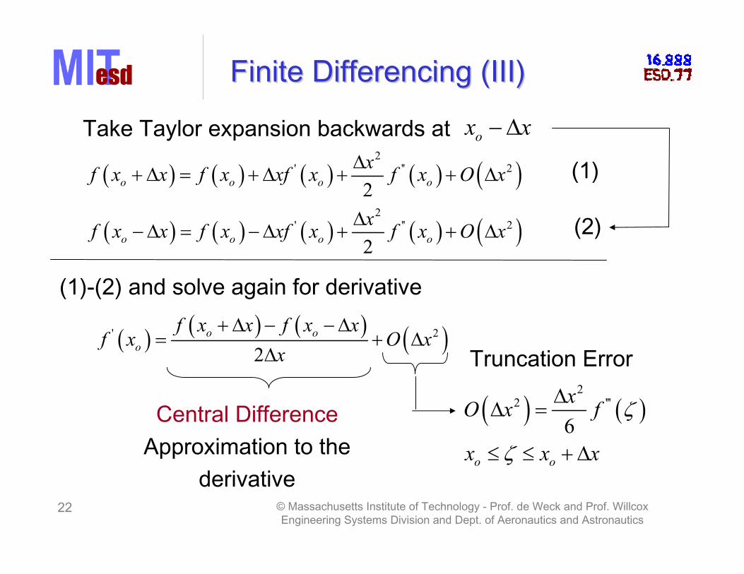
Finite Differencing (III)Finite Differencing (III)
Take Taylor expansion backwards at ox x
2' '' 2
2o o o o
xf x x f x xf x f x O x
2' '' 2
2o o o o
xf x x f x xf x f x O x (1)
(2)
(1)-(2) and solve again for derivative
' 2
2o o
o
f x x f x xf x O x
x
22 '''
6
o o
xO x f
x x x
Truncation Error
Central DifferenceApproximation to the
derivative

23 © Massachusetts Institute of Technology - Prof. de Weck and Prof. WillcoxEngineering Systems Division and Dept. of Aeronautics and Astronautics
Finite Difference OverviewFinite Difference Overview
xForward Difference
'( ) o oo
f x x f xf x
x
1st derivative 2nd derivative
2
2 2''( ) o o o
o
f x x f x x f xf x
x
xx
Central Difference2nd derivative1st derivative
'( )2
o oo
f x x f x xf x
x2
2''( ) o o o
o
f x x f x f x xf x
x
24 © Massachusetts Institute of Technology - Prof. de Weck and Prof. WillcoxEngineering Systems Division and Dept. of Aeronautics and Astronautics
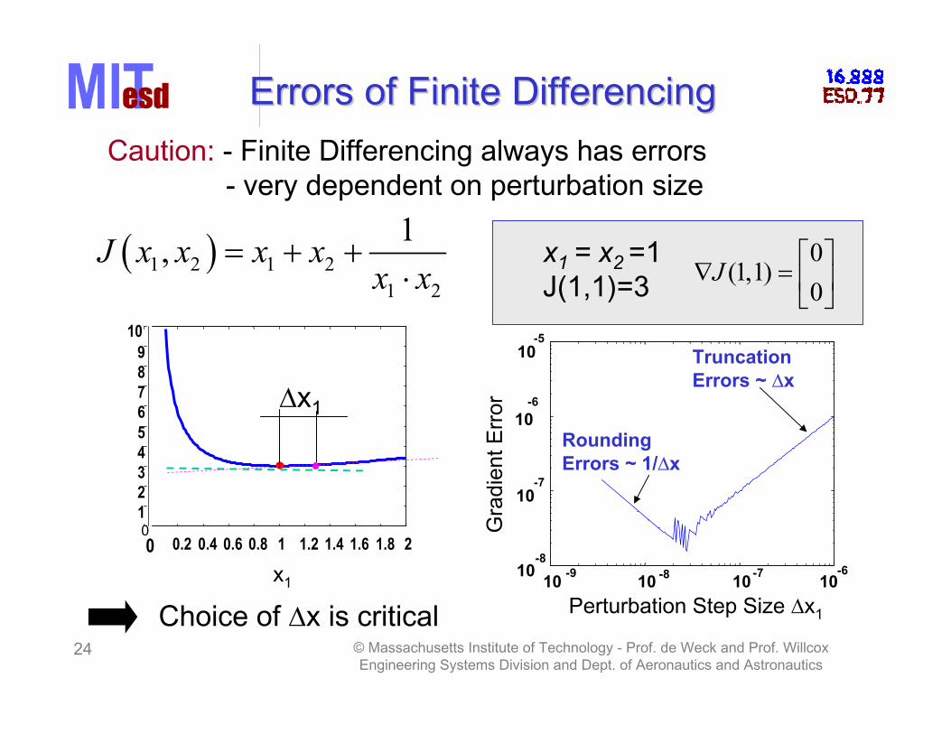
Errors of Finite DifferencingErrors of Finite DifferencingCaution: - Finite Differencing always has errors
- very dependent on perturbation size
1 2 1 21 2
1,J x x x x
x xx1 = x2 =1J(1,1)=3
0(1,1)
0J
0 0.2 0.4 0.6 0.8 1 1.2 1.4 1.6 1.8 20123456789
10
x1
x1
10 -9 10 -8 10-7 10-610
-8
10-7
10-6
10-5
TruncationErrors ~ x
RoundingErrors ~ 1/ x
Perturbation Step Size x1
Gra
dien
t Err
or
Choice of x is critical

25 © Massachusetts Institute of Technology - Prof. de Weck and Prof. WillcoxEngineering Systems Division and Dept. of Aeronautics and Astronautics
Perturbation Size Perturbation Size x Choicex Choice
• Error Analysis
• Significant digits (Barton 1992)
• Machine Precision
• Trial and Error – typical value ~ 0.1-1%
1/ 2
Ax f - Forward difference1/3
Ax f - Central difference
(Gill et al. 1981)
ox
theoretical function
computedvalues
~ x
A
10 qk kx xStep size
at k-th iterationq-# of digits of machinePrecision for real numbers

26 © Massachusetts Institute of Technology - Prof. de Weck and Prof. WillcoxEngineering Systems Division and Dept. of Aeronautics and Astronautics
Computational Expense of FDComputational Expense of FD
Cost of a single objective functionevaluation of Ji
iF J
Cost of gradient vector finitedifference approximation for Jifor a design vector of length n
in F J
Cost of Jacobian finitedifference approximation with z objective functions
iz n F J
Example: 6 objectives30 design variables1 sec per simcode evaluation
3 min of CPU timefor a single Jacobianestimate - expensive !
27 © Massachusetts Institute of Technology - Prof. de Weck and Prof. WillcoxEngineering Systems Division and Dept. of Aeronautics and Astronautics
Automatic DifferentiationAutomatic Differentiation
• Mathematical formulas are built from a finite set of basic functions, e.g. sin x, cos x, exp x
• Take analysis code in C or Fortran
• Using chain rule, add statements that generate derivatives of the basic functions
• Tracks numerical values of derivatives, does not track symbolically as discussed before
• Outputs modified program = original + derivative capability
28 © Massachusetts Institute of Technology - Prof. de Weck and Prof. WillcoxEngineering Systems Division and Dept. of Aeronautics and Astronautics
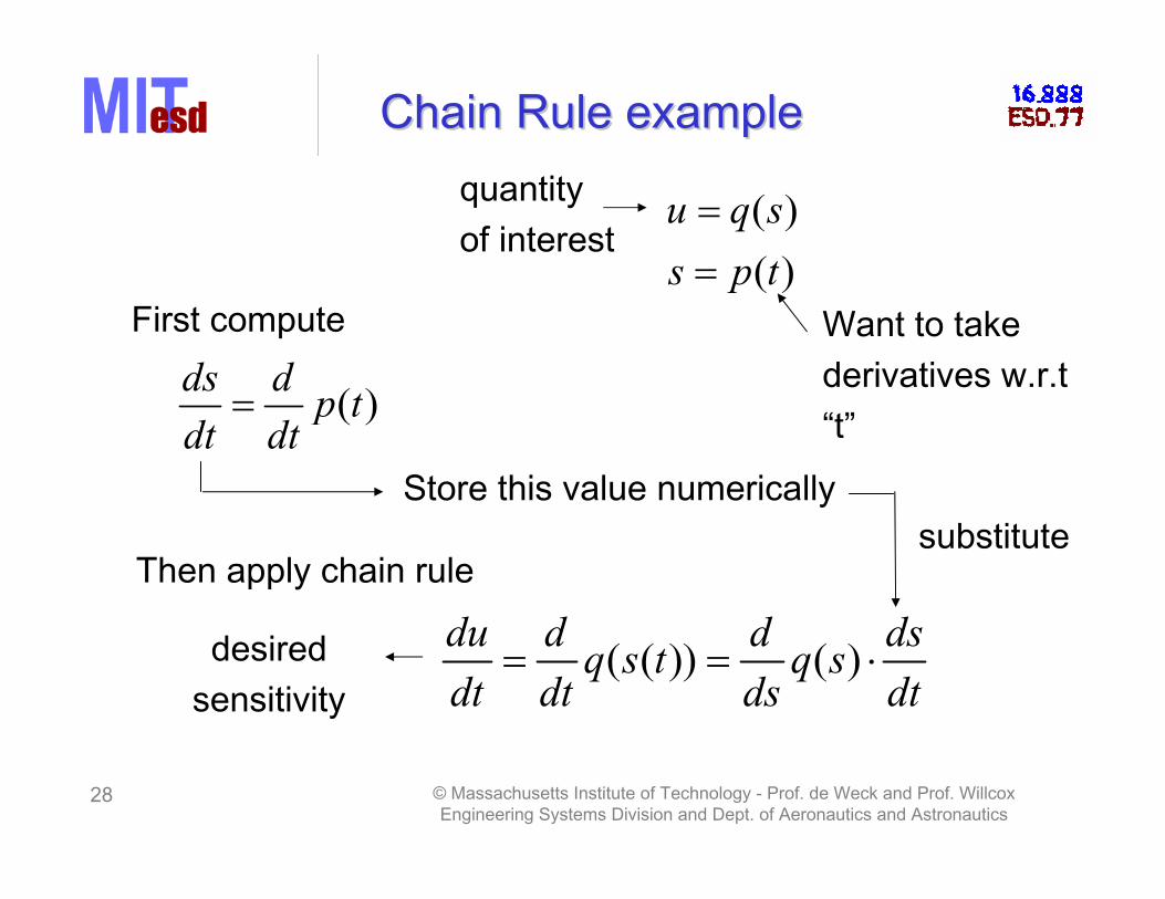
Chain Rule exampleChain Rule example
( )
( )
u q s
s p t
quantityof interest
First compute Want to takederivatives w.r.t “t”
( )ds d
p tdt dt
Store this value numerically
Then apply chain rule
( ( )) ( )du d d ds
q s t q sdt dt ds dt
substitute
desiredsensitivity

29 © Massachusetts Institute of Technology - Prof. de Weck and Prof. WillcoxEngineering Systems Division and Dept. of Aeronautics and Astronautics
Chain Rule Coding ExampleChain Rule Coding Example
hr = gm*eps/rho-0.5*g1*(ux*ux + vy*vy);
h_u[0] = -gm*eps/(rho*rho);
h_u[1] = -g1*ux;
h_u[2] = -g1*vy;
h_u[3] = gm/rho;
hi = (di*hr+hl)*d1;
hi_u[0] = (di*hr+hl)*d1_u[0]
+ d1*(di_u[0]*hr+di*h_u[0]);
• compute hrdifferentiate:• wrt rho• wrt ux• wrt vy• wrt eps

30 © Massachusetts Institute of Technology - Prof. de Weck and Prof. WillcoxEngineering Systems Division and Dept. of Aeronautics and Astronautics
Adjoint MethodsAdjoint Methods
• A way to get gradient information in a computationally efficient way
• Based on theory from controls• Applied extensively in aerodynamic design and
optimization• For example, in aerodynamic shape design, need
objective gradient with respect to shape parameters andwith respect to flow parameters
– Would be expensive if finite differences are used!• Adjoint methods have allowed optimization to be used
for complicated, high-fidelity fluids problems.
31 © Massachusetts Institute of Technology - Prof. de Weck and Prof. WillcoxEngineering Systems Division and Dept. of Aeronautics and Astronautics
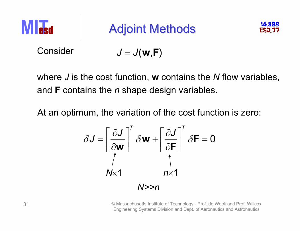
Adjoint MethodsAdjoint Methods
Consider
where J is the cost function, w contains the N flow variables,and F contains the n shape design variables.
( , )J J w F
At an optimum, the variation of the cost function is zero:
0T T
J JJ w F
w F
N 1 n 1
N>>n

32 © Massachusetts Institute of Technology - Prof. de Weck and Prof. WillcoxEngineering Systems Division and Dept. of Aeronautics and Astronautics
Adjoint MethodsAdjoint Methods
Fluid governing equations: ( , ) 0R w F
0R R
R w Fw F
We can append these constraints to the cost function using a Lagrange multiplier approach:
T
T T
T T
T T
J J R RJ
J R J R
w F w Fw F w F
w Fw w F F

33 © Massachusetts Institute of Technology - Prof. de Weck and Prof. WillcoxEngineering Systems Division and Dept. of Aeronautics and Astronautics
Adjoint MethodsAdjoint Methods
T TT T
J R J RJ w F
w w F F
Choose to satisfy the adjoint equation: T
R Jw w
equivalent to one flow solve
TT
J RJ F
F FThen does not depend
on the number of flow variables
total gradient of J
34 © Massachusetts Institute of Technology - Prof. de Weck and Prof. WillcoxEngineering Systems Division and Dept. of Aeronautics and Astronautics
Sensitivity AnalysisSensitivity Analysis
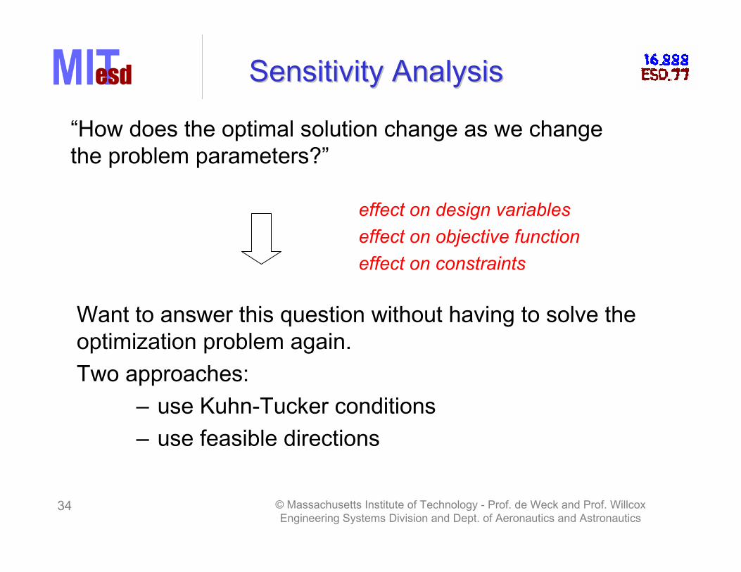
“How does the optimal solution change as we change the problem parameters?”
effect on design variableseffect on objective functioneffect on constraints
Want to answer this question without having to solve the optimization problem again.Two approaches:
– use Kuhn-Tucker conditions– use feasible directions

35 © Massachusetts Institute of Technology - Prof. de Weck and Prof. WillcoxEngineering Systems Division and Dept. of Aeronautics and Astronautics
ParametersParameters
Parameters p are the fixed assumptions.How sensitive is the optimal solution x* with respectto fixed parameters ?
Optimal solution:
x* =[ R=106.1m, L=0m, N=17 cows]TExample:
“Dairy Farm” sample problem
L
R N
fence
Fixed parameters:
Parameters:f=100$/m - Cost of fencen=2000$/cow - Cost of a single cowm=2$/liter - Market price of milk
How does x* change as parameterschange?
Maximize Profit
COW
COW COW

36 © Massachusetts Institute of Technology - Prof. de Weck and Prof. WillcoxEngineering Systems Division and Dept. of Aeronautics and Astronautics
Sensitivity AnalysisSensitivity Analysis
Recall the Kuhn-Tucker conditions. Let us assume that we have M active constraints, which are contained in the vector
*ˆ( *) ( ) 0
ˆ ( *) 0,
0,
j jj M
j
j
J g
g j M
j M
x x
x
ˆ( )g x
For a small change in a parameter, p, we require that the Kuhn-Tucker conditions remain valid:
(KT conditions)0
ddp

37 © Massachusetts Institute of Technology - Prof. de Weck and Prof. WillcoxEngineering Systems Division and Dept. of Aeronautics and Astronautics
Sensitivity AnalysisSensitivity Analysis
First, let us write out the components of the first equation:
* *ˆ( ) ( ) 0j jj M
J gx x
* *ˆ
( ) ( ) 0, 1,...,jj
j Mi i
gJi n
x xx x
Now differentiate with respect to the parameter p usingthe chain rule:
1
ni
k i
dY Y Y xdp p x p

38
© Massachusetts Institute of Technology - P
Prof. de Weck and Prof. WillcoxEngineering Systems Division and Dept. of Aeronautics and Astronautics
Sensitivity AnalysisSensitivity Analysis
* *ˆ
( ) ( ) 0jj
j Mi i
gJx x
x x ˆ ( *) 0jg x
differentiate wrt p:
22
1
22
ˆ
ˆ ˆ0
nj k
jk j Mi k i k
j j j
j M j Mi i i
gJ xx x x x p
g gJx p x p x p
1
ˆ ˆ0
nj j k
k k
g g xp x p
unknowns are and jixp p

39 © Massachusetts Institute of Technology - Prof. de Weck and Prof. WillcoxEngineering Systems Division and Dept. of Aeronautics and Astronautics
Sensitivity AnalysisSensitivity AnalysisIn matrix form we can write:
00T
A B c
B d
xn
M
Mn
22 ˆ jik j
j Mi k i k
gJA
x x x xˆ j
iji
gB
x22 ˆ j
ij Mi i
gJc
x p x pˆ j
j
gd
p
1
2
n
xp
xp
xp
x
1
2
M
p
p
p

40 © Massachusetts Institute of Technology - Prof. de Weck and Prof. WillcoxEngineering Systems Division and Dept. of Aeronautics and Astronautics
Sensitivity AnalysisSensitivity Analysis
We solve the system to find x and , then the sensitivity of the objective function with respect to p can be found:
TdJ JJ
dp px
dJJ p
dp(first-order
approximation)
px x
To assess the effect of changing a different parameter, we only need to calculate a new RHS in the matrix system.
41 © Massachusetts Institute of Technology - Prof. de Weck and Prof. WillcoxEngineering Systems Division and Dept. of Aeronautics and Astronautics
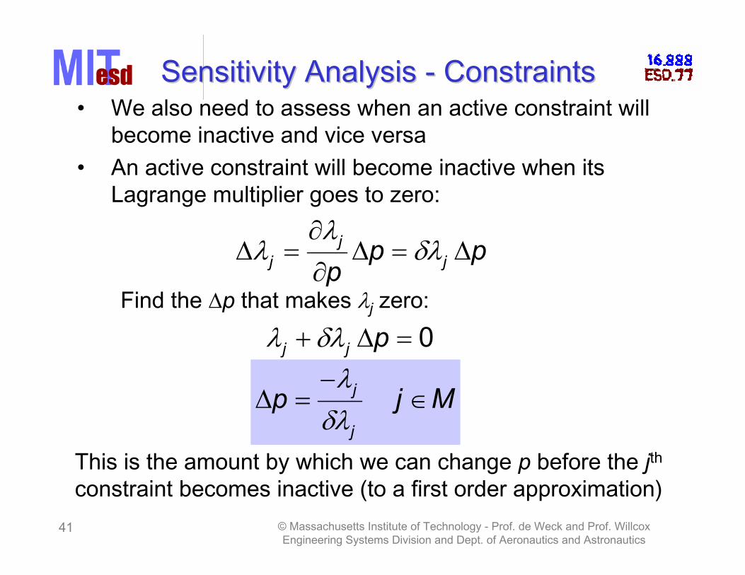
Sensitivity Analysis Sensitivity Analysis -- ConstraintsConstraints• We also need to assess when an active constraint will
become inactive and vice versa• An active constraint will become inactive when its
Lagrange multiplier goes to zero:
jj jp p
pFind the p that makes j zero:
0j j p
j
j
p j M
This is the amount by which we can change p before the jth
constraint becomes inactive (to a first order approximation)

42 © Massachusetts Institute of Technology - Prof. de Weck and Prof. WillcoxEngineering Systems Division and Dept. of Aeronautics and Astronautics
Sensitivity Analysis Sensitivity Analysis -- ConstraintsConstraintsAn inactive constraint will become active when gj(x)goes to zero:
( ) ( *) ( *) 0Tj j jg g p gx x x x
Find the p that makes gj zero:
( *)
( *)j
Tj
gp
g
xx x
for all j notactive at x*
• This is the amount by which we can change p before the jth
constraint becomes active (to a first order approximation)• If we want to change p by a larger amount, then the problem
must be solved again including the new constraint• Only valid close to the optimum

43 © Massachusetts Institute of Technology - Prof. de Weck and Prof. WillcoxEngineering Systems Division and Dept. of Aeronautics and Astronautics
Lecture SummaryLecture Summary
• Sensitivity analysis– Yields important information about the design space,
both as the optimization is proceeding and once the “optimal” solution has been reached.
• Gradient calculation approaches– Analytical and Symbolic– Finite difference– Automatic Differentiation– Adjoint methods
ReadingPapalambros – Section 8.2 Computing Derivatives
Top Related