


Languages
Pages
Legal


394
Multi-Objective Design Optimization of a Rudder, using Automated
CAE Model Set-Up with ANSA Pre-Processor
George Korbetis, BETA CAE Systems S.A., Thessaloniki/Greece, [email protected]
Dimitris Georgoulas, BETA CAE Systems S.A., Thessaloniki/Greece, [email protected]
Abstract
Components of great importance for the ship safety are subjected to extensive analyses to ensure
minimum failure risk and high performance. In such cases, the design process involves Finite Element
Method simulations with which the model behavior for several loading conditions is evaluated.
Analysts need to provide feedback to the designers regarding the simulation results and propose
design changes towards the achievement of the required product’s performance characteristics.
Following that, the designers have to propagate the proposed changes by updating the products
geometry. The automated definition of the CAE simulation model becomes essential during the above
design loop, because a great amount of engineering hours are saved. Through an automated process,
the analyst is able to produce CAE models for various disciplines and load cases, which are updated
for each design change of the product. This paper presents the implementation of an automated
process for the definition of a CAE model of a spade rudder with rudder trunk and the strength
analysis of it. The automated CAE model set-up capability of ANSA pre-processor is used to define
CAE models for static, contact and CFD analyses. ANSA, and µETA post-processor, which is
exploited for the extraction of responses from the solver results, are coupled to the modeFRONTIER
optimizer for the identification of the best rudder shape.
1. Introduction
The use of the Finite Elements Analysis becomes increasingly popular in marine design, since it can
give us valuable information on the strength, hydrodynamics, and model behavior of complicated
parts and assemblies. However it is always time consuming to set up and standardize a simulation
process within the design process. The pre- and post- processors of BETA CAE Systems, ANSA and
µETA, provide sophisticated tools in order to facilitate the FEA process. Time consuming tasks like
meshing, model simplification and mesh quality improvement have been replaced by automated
processes which save a lot of engineer working hours. Additionally, such tools guide the engineer to
set up the model in the most proper way and help him to overcome any human errors.
This paper demonstrates the suggested process of the definition of a strength analysis and the
application of the multi objective optimization during the design process on a ship’s rudder. A
simplified CFD (computational fluid dynamics) analysis calculates the maximum force applied on the
rudder’s surface. The calculated force is taken as the loading condition for the rudder’s structural
analysis. The static analysis is set up using automated processes like the results mapping, the contact
pair definition and the batch meshing which are provided by ANSA. Model shape parameterization is
performed by the ANSA Morphing Tool and the Optimization Task and different design variables are
defined to control the model. To investigate the model behavior, the structural analysis is coupled
with an optimization process. The first step of this process identifies the critical variables of the
increase of the model’s strength, while a second step performs a multi-objective optimization to find
the best combination of the input variables.
2. Problem definition
The case study model is a spade rudder with rudder trunk of a Handysize bulk carrier. The ship’s
length is 169 m and its maximum speed 15 knots. When the ship is fully loaded the whole rudder and
skeg are submerged beneath the sea. The rudder cross section is NACA 0015 and its main dimensions
are x1=3.56 m, x2=5.05 m, b=6.2 and A=26.7 m2, Fig.1. The rudder and stock material is steel with
Young’s Modulus 210 GPa, Yield stress 235 MPa and density 7.86⋅10-6
Kg/mm2.

Fig.1: Rudder sketch
The stock is supported by a THORDON elastomeric bearing of type SLX assembled on the rudder
truck. It is connected to the rudder’s body by a cone coupling which is welded on the body. The stock
uppermost part is clamped to a rotary valve which drives the rudder. The elastomeric bearing’s
Young’s Modulus is 440 MPa, its maximum working contact pressure 10-12 MPa.
The main force that strains the rudder is produced by the water flow around it. The maximum force
appears at the vessel’s full speed, when the rudder turns to the maximum angle of 35°. The weight and
buoyancy are considerably small in relation to the water flow force; therefore they are not taken into
account. To evaluate the force that is distributed to the whole surface of the rudder, a CFD analysis is
performed. The results from the CFD analysis are used as boundary conditions to the structural
analysis of the rudder assembly.
3. Model set-up
Two different FE models should be prepared for the structural and CFD analyses. Both models are
created by the initial geometry, however, different representations are defined for each model. Each
representation contains only the needed parts and entities for each analysis and the proper meshing
parameters, quality criteria, boundary conditions and auxiliary geometry (i.e. fluid domain). The
geometrical model is shown in Fig.2.
Fig.2: Geometrical model
x2
b1
x1
A

3.1. CFD analysis
The first load case is a CFD analysis performed in order to evaluate the pressure on the rudder body.
The first estimation of the pressure is done using a simplified model of the rudder. The effect of hull
and propeller on the water flow is not taken into account for this case study and the flow is considered
steady. For the definition of the CFD model, the outer skin of the rudder is isolated from the
geometrical model and assembled to the computational domain which represents an open ocean area.
3.1.1. Meshing definition
The rudder’s surface is meshed with a variable size triangular mesh. The boundary layer, generated on
the rudder and the fluid surface separation, consists of five layers of prisms, generated in absolute
mode with a growth factor of 1.2 and first height of 5 mm. A tetra mesh was generated on the fluid
domain with element length varying from 0.05 to 2 m. In the fluid domain and more specifically on
the area around the rudder, a fine mesh is required to increase the result’s accuracy. In this case a
special entity of ANSA, the Size Box, is defined in this area which constrains the element length of
the fluid domain that resides inside the Size Box volume at 0.1 m. The final model consists of
approximately 3,000,000 elements, Fig.3. The mesh is applied automatically on the model and fluid
domain through the ANSA Batch Meshing Tool.
Fig.3: CFD mesh
3.1.2. Results in META
For the CFD analysis, ANSYS FLUENT v13.0 is used. After about 1000 iterations conversion is
achieved. The static pressure is exported in ABAQUS format in order to feed the static analysis that
will take place later on.
The results of the solution can be viewed and evaluated through µETA (ver. 6.7.2), which supports
the read in of numerous CFD solvers results. As expected, the flow separates early on the rudder’s
surface, since the angle of attack is considerably high. µETA offers many ways to view CFD results
such as streamlines, vectors and contours as shown in Figs.4 to 7 and is capable of calculating many
factors and values like the Cd and Cl factors and the Yplus values.

Fig.4: Velocity in streamlines Fig.5: Yplus in contour plot
Fig.6: Pressure in contour plot Fig.7: Vorticity in contour plot
3.2. The static analysis
The second analysis calculates the strength of the rudder assembly and the contact pressure between
the bearing and the stock. The analysis is static, nonlinear and it is set up for the Abaqus 6.10. The
representation of the geometrical model that participates in the analysis is shown in Fig.8.
Fig.8: Structural model

3.2.1. Meshing definition
The rudder assembly is meshed with 1st order shell elements of mean element length 50 mm. Special
treatment is prescribed for holes where on these perimeters one zone of elements is applied. The
quality criteria that are used are listed on Table I. For the meshing process the ANSA Batch Meshing
Tool is used. In this tool the meshing parameters and quality criteria are prescribed for a meshing
scenario which is applied on the thin wall parts of the rudder and skeg. One more meshing scenario is
defined for the cone coupling. In that case three layers of PENTAS are created on the part’s conical
surface to ensure successful coupling with the stock, since penetration problems and difficulty to
converge may occur during solution. Above the layers, first-order solid elements (TETRAS) are
prescribed for the rest of the solid part. The Batch Meshing Tool runs and applies meshing and quality
improvement on all selected parts, according to the prescribed meshing scenarios without the need of
any user interaction. The meshed parts are shown in Figs.9 to 11.
Table I: Rudder meshing specifications
Quality criteria Shells Solids Calculation
Aspect ratio 3 Abaqus
Skewness 0.8 0.6 Abaqus
Warping 10 Ideas
Min. Length 15 15
Max. Length 70 70
Min. Angle Quads 45 Abaqus
Max. Angle Quads 135 Abaqus
Min. Angle Trias 30 Abaqus
Max. Angle Trias 120 Abaqus
Fig.9: Rudder body mesh Fig.10: Rudder skeg mesh
The rudder stock and the bearing are parts of great importance for this analysis and their results need
to be accurate. Thus, thin layers of HEXA elements are applied on the stock perimeter to ensure
accuracy of the desired results. In addition, the whole stock model is meshed with HEXA elements.
The HEXA meshing process is a semi-automatic process in ANSA since special entities, the Hexa
Boxes, are created around the stock model. Each box represents a meshing domain, in which meshing
parameters, such as node number, spacing and number of layers are defined. After the definition of
the Hexa Boxes the mesh is created automatically. Three layers of HEXA elements are applied on the
stock / bearing contact area with element length of 4.5 mm, while the rest of the part is meshed with
30 mm HEXA elements, Fig.12. The bearing is also meshed with HEXA elements. Since its geometry
is very simple there is no need to use the Hexa Boxes, Fig.13.

Fig.11: Cone coupling mesh
Fig.12: The stock mesh Fig.13: The bearing mesh
3.2.2. Defining boundary conditions
The structural analysis is limited to the rudder assembly, so the rest of the ship is considered rigid.
Thus, boundary conditions are applied on the upper nodes of the rudder skeg which constrain the
displacement and rotation in all degrees of freedom, Fig.14.
Fig.14: Boundary constraints of skeg Fig.15: Boundary constraints of stock
BOUNDARY
MPCs

The rotary valve is also considered as rigid body. The latter constrains the displacement of the stock at
all axes and the rotation of the Z axis. To represent this constraint, a BOUNDARY entity of Abaqus is
created in the center of the coupling which is connected to the stock coupling surface using rigid MPC
elements, Fig.15.
3.2.3. Automatic definition of contacts
The rudder stock is connected to the rudder by the cone coupling and supported on the rudder trunk
by the elastomeric bearing. These connections are simulated by CONTACT PAIR entities according
to Abaqus, in order to evaluate the pressure that occurs on the contact surfaces during loading. A
special tool of ANSA for this purpose identifies the mating surfaces of the candidate pairs so that the
user can decide whether to accept them and define the type of the coupling. Two contact pairs
represent the coupling of the stock with the cone flange, Fig.16. The type of the above pairs is defined
as TIE according to Abaqus, since no movement is expected in this area. The contact pair between the
stock and the bearing is defined as CONTACT, according to Abaqus, since the connection is not fixed
and small sliding is allowed, Fig.17. In this case, the actual area of contact and the distribution of the
pressure depend on the load case and the rigidity of the stock, trunk and bearing. A friction model is
applied with friction coefficient of 0.2.
Fig.16: Contact between cone coupling and stock Fig.17: Contact between bearing and stock
Fig.18: Mapping pressure from CFD to static models

3.2.4. Mapping the CFD results
The pressure applied on the rudder’s surface, which is calculated by the CFD analysis, is considered
as the loading condition for the static analysis. Therefore, the pressure results are exported from
Fluent to an Abaqus format file containing pressure values for each element. However, the mesh of
the rudder for the CFD analysis is not compatible with the one for the static analysis. In this case, the
pressure derived from the CFD analysis is mapped to the static analysis mesh by regenerating
equivalent pressure entities to the target elements. This is achieved with the use of the ANSA Results
Mapper, which is able to import results of any type from numerous solvers, Fig.18. To complete the
FE model that will be exported to Abaqus, the proper materials, shell and solid properties and header
are defined. Output requests are defined for strain, stress and contact pressure.
4. Optimization problem
An initial run of the FE Model reveals the parts and areas where maximum stress and pressure appear.
The µETA post-processor is used to identify the critical areas and create reports and statistics for all
parts. As shown in the following figures the maximum value for the Von Misses stress occurs on the
rudder trunk near to the supporting webs. The value 215 MPa which is close to the Yield stress makes
the increase of the truck’s thickness essential. Contact pressure results are read in µETA for the
bearing - stock coupling. The maximum pressures appear close to the bearing’s lower edge, Fig.20.
The maximum pressure value is 9 MPa which is acceptable. However, more uniform pressure
distribution is desired. Furthermore, the deflection of the rudder is measured at the lower nodes of the
model which is 32.4 mm.
Fig.19: Von Misses stress at rudder trunk Fig.20: Contact pressure at bearing
Fig.21: Deflection at rudder body Fig.22: Von Misses Stress at stock

In this case study the model’s behavior can be improved by modifying certain parameters that
correspond to the model’s shape and shell thickness. The target of the optimization is to minimize the
contact pressure on the bearing and the deflection of the rudder body. The maximum stress and the
total rudder mass should be kept within an acceptable range. The model’s improvement is performed
in two steps. First, a statistical analysis indicates which of the variables have big influence on the
model’s behavior and which would be the appropriate design space. Furthermore, a multi objective
optimization searches for the optimum solution.
4.1. Defining morphing parameters
The shaping of the geometrical or FE model is achieved by the ANSA Morphing Tool. This tool
provides several ways of morphing while ensuring smooth and controllable results. Special entities,
the Morphing Boxes, are created around the area of the model to be modified. As the shape of the
Morphing Boxes can be modified in several ways, the model surrounded by the Boxes follows the
modification. Thus, the shaping takes place. Morphing should be performed parametrically in order to
be driven by the optimization process. In this case Morphing Parameters which control the Morphing
Boxes and are connected to the design variables of the optimization problem are defined. Several
Morphing Parameters which control modifications of the model shape will be defined, Table II. Their
bounds are prescribed according to the minimum / maximum permissible values that derive from
technical specifications, model geometry and manufacturability.
Table II: The Morphing Parameters
Design Variable Minimum Initial Maximum
Bearing Outer Radius 302 350 350
Bearing Inner Radius 265 275 275
Bearing Length -300 0 300
Stock Radius 235 235 260
Holes Radius -50 0 34
Vertical Web Move 1 -290 0 45
Vertical Web Move 2 -100 0 200
Trunk Support Webs 10 18 25
Trunk 10 20 25
Rudder Blade Skin 10 15 20
Rudder Horizontal Webs 10 15 20
Rudder Vertical Webs 10 15 20
For the modification of the stock geometry Cylindrical Morphing Boxes are used which are ideal for
axi-symmetric models and the relative Morphing Parameters which control stock diameter between
rotary valve coupling and bearing, Fig.23. The same group of Cylindrical Morphing Boxes also
controls the thickness and length of the bearing using respective Morphing Parameters.
Fig.23: Cylindrical Morphing Boxes on the stock
bearing diameter
bearing length
stock diameter
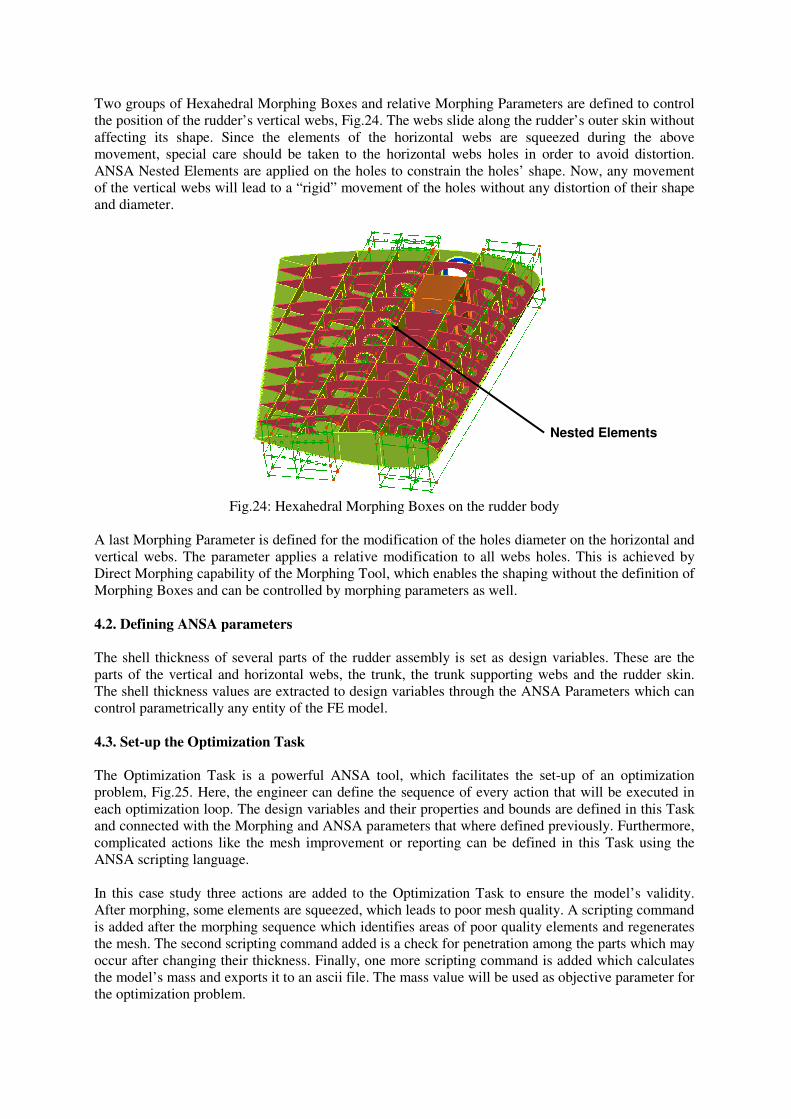
Two groups of Hexahedral Morphing Boxes and relative Morphing Parameters are defined to control
the position of the rudder’s vertical webs, Fig.24. The webs slide along the rudder’s outer skin without
affecting its shape. Since the elements of the horizontal webs are squeezed during the above
movement, special care should be taken to the horizontal webs holes in order to avoid distortion.
ANSA Nested Elements are applied on the holes to constrain the holes’ shape. Now, any movement
of the vertical webs will lead to a “rigid” movement of the holes without any distortion of their shape
and diameter.
Fig.24: Hexahedral Morphing Boxes on the rudder body
A last Morphing Parameter is defined for the modification of the holes diameter on the horizontal and
vertical webs. The parameter applies a relative modification to all webs holes. This is achieved by
Direct Morphing capability of the Morphing Tool, which enables the shaping without the definition of
Morphing Boxes and can be controlled by morphing parameters as well.
4.2. Defining ANSA parameters
The shell thickness of several parts of the rudder assembly is set as design variables. These are the
parts of the vertical and horizontal webs, the trunk, the trunk supporting webs and the rudder skin.
The shell thickness values are extracted to design variables through the ANSA Parameters which can
control parametrically any entity of the FE model.
4.3. Set-up the Optimization Task
The Optimization Task is a powerful ANSA tool, which facilitates the set-up of an optimization
problem, Fig.25. Here, the engineer can define the sequence of every action that will be executed in
each optimization loop. The design variables and their properties and bounds are defined in this Task
and connected with the Morphing and ANSA parameters that where defined previously. Furthermore,
complicated actions like the mesh improvement or reporting can be defined in this Task using the
ANSA scripting language.
In this case study three actions are added to the Optimization Task to ensure the model’s validity.
After morphing, some elements are squeezed, which leads to poor mesh quality. A scripting command
is added after the morphing sequence which identifies areas of poor quality elements and regenerates
the mesh. The second scripting command added is a check for penetration among the parts which may
occur after changing their thickness. Finally, one more scripting command is added which calculates
the model’s mass and exports it to an ascii file. The mass value will be used as objective parameter for
the optimization problem.
Nested Elements

Fig.25: Optimization task
4.4. Extracting responses from META
The objective parameters and constraints of the optimization problem are extracted from the results of
the structural simulation. To achieve this, a baseline run of the static analysis is performed and the
results are read in µETA. Through the Annotation tool of µETA, the maximum value of the contact
pressure on the bearing and the maximum stress and deflection on the rudder assembly are identified.
The OptimizerSetup tool of µETA is used to export the identified values into an ascii file of a special
format, Fig.26. The file is read from modeFRONTIER, www.modefrontier.com, and the values are set
as responses. The above sequence, of extracting the responses, is recorded automatically in a session
file in order to be reproduced in every optimization loop.
Fig.26: OptimizerSetup Tool
4.5. Coupling ANSA / META to modeFRONTIER
For this optimization problem the modeFRONTIER 4.4.1 is used which provides dedicated “nodes”
for ANSA and µETA. Thus, the coupling of the pre- and post- processing sequence is done without
the need of any scripting or customization. As the ANSA node is defined, the input variables are
automatically defined corresponding to the Design Variables that have been set in the ANSA
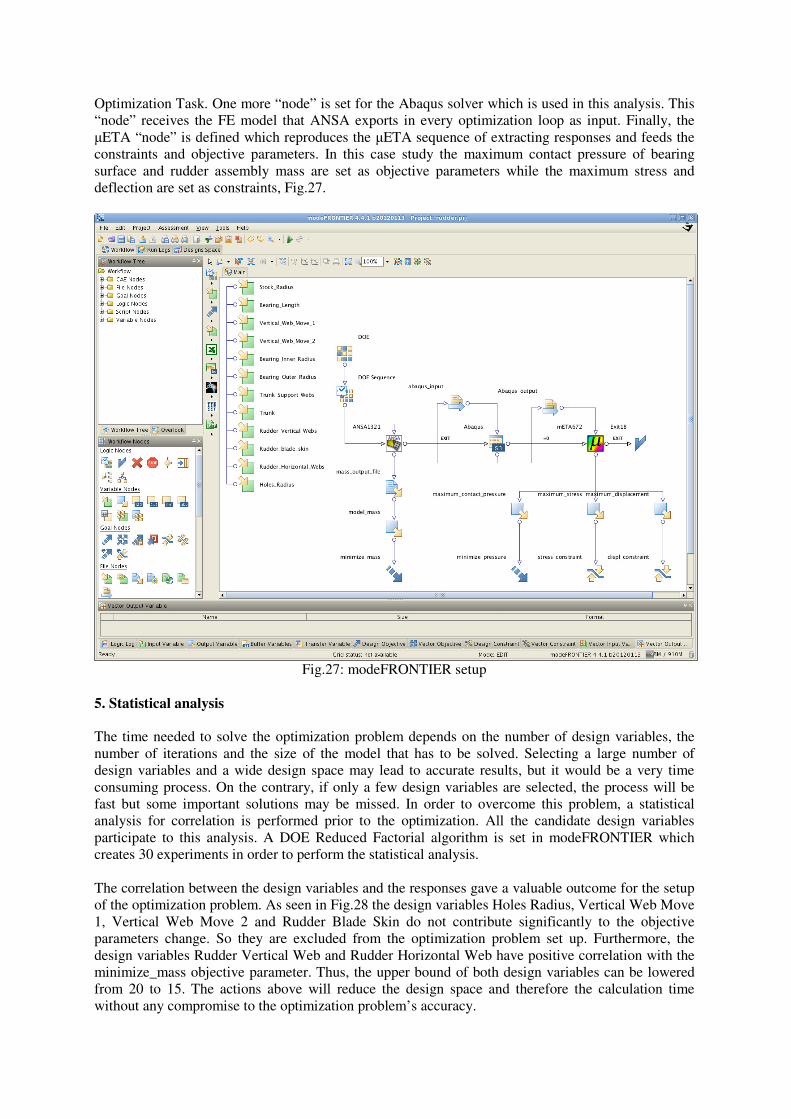
Optimization Task. One more “node” is set for the Abaqus solver which is used in this analysis. This
“node” receives the FE model that ANSA exports in every optimization loop as input. Finally, the
µETA “node” is defined which reproduces the µETA sequence of extracting responses and feeds the
constraints and objective parameters. In this case study the maximum contact pressure of bearing
surface and rudder assembly mass are set as objective parameters while the maximum stress and
deflection are set as constraints, Fig.27.
Fig.27: modeFRONTIER setup
5. Statistical analysis
The time needed to solve the optimization problem depends on the number of design variables, the
number of iterations and the size of the model that has to be solved. Selecting a large number of
design variables and a wide design space may lead to accurate results, but it would be a very time
consuming process. On the contrary, if only a few design variables are selected, the process will be
fast but some important solutions may be missed. In order to overcome this problem, a statistical
analysis for correlation is performed prior to the optimization. All the candidate design variables
participate to this analysis. A DOE Reduced Factorial algorithm is set in modeFRONTIER which
creates 30 experiments in order to perform the statistical analysis.
The correlation between the design variables and the responses gave a valuable outcome for the setup
of the optimization problem. As seen in Fig.28 the design variables Holes Radius, Vertical Web Move
1, Vertical Web Move 2 and Rudder Blade Skin do not contribute significantly to the objective
parameters change. So they are excluded from the optimization problem set up. Furthermore, the
design variables Rudder Vertical Web and Rudder Horizontal Web have positive correlation with the
minimize_mass objective parameter. Thus, the upper bound of both design variables can be lowered
from 20 to 15. The actions above will reduce the design space and therefore the calculation time
without any compromise to the optimization problem’s accuracy.

Fig.28: Statistical analysis results
6. Performing optimization
After the final adjustment of the design variables, the optimization problem is set up. The Multi
Objective Genetic Algorithm (MOGA II) is selected and the process runs for 360 iterations. The
feasible iterations are shown in the contact pressure vs. mass diagram, Fig.29, in grey color while
unfeasible ones in white. The bubbles diameter represents the maximum stress. The Pareto Frontier
appears which shows the best solutions for this case study. The optimum solution reduces contact
pressure for 12.5% and the mass for 7.98% while the maximum stress and the displacement are kept
below the acceptable values, Table III. The design variables values for the optimum solution are
shown on Table IV.
Fig.29: The contact pressure vs. mass diagram
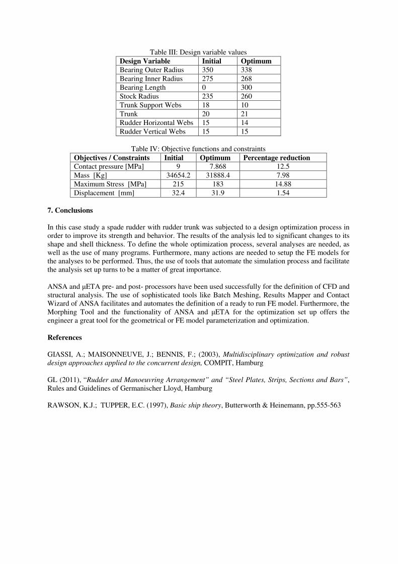
Table III: Design variable values
Design Variable Initial Optimum
Bearing Outer Radius 350 338
Bearing Inner Radius 275 268
Bearing Length 0 300
Stock Radius 235 260
Trunk Support Webs 18 10
Trunk 20 21
Rudder Horizontal Webs 15 14
Rudder Vertical Webs 15 15
Table IV: Objective functions and constraints
Objectives / Constraints Initial Optimum Percentage reduction
Contact pressure [MPa] 9 7.868 12.5
Mass [Kg] 34654.2 31888.4 7.98
Maximum Stress [MPa] 215 183 14.88
Displacement [mm] 32.4 31.9 1.54
7. Conclusions
In this case study a spade rudder with rudder trunk was subjected to a design optimization process in
order to improve its strength and behavior. The results of the analysis led to significant changes to its
shape and shell thickness. To define the whole optimization process, several analyses are needed, as
well as the use of many programs. Furthermore, many actions are needed to setup the FE models for
the analyses to be performed. Thus, the use of tools that automate the simulation process and facilitate
the analysis set up turns to be a matter of great importance.
ANSA and µETA pre- and post- processors have been used successfully for the definition of CFD and
structural analysis. The use of sophisticated tools like Batch Meshing, Results Mapper and Contact
Wizard of ANSA facilitates and automates the definition of a ready to run FE model. Furthermore, the
Morphing Tool and the functionality of ANSA and µETA for the optimization set up offers the
engineer a great tool for the geometrical or FE model parameterization and optimization.
References
GIASSI, A.; MAISONNEUVE, J.; BENNIS, F.; (2003), Multidisciplinary optimization and robust
design approaches applied to the concurrent design, COMPIT, Hamburg
GL (2011), “Rudder and Manoeuvring Arrangement” and “Steel Plates, Strips, Sections and Bars”,
Rules and Guidelines of Germanischer Lloyd, Hamburg
RAWSON, K.J.; TUPPER, E.C. (1997), Basic ship theory, Butterworth & Heinemann, pp.555-563
Top Related