


Languages
Pages
Legal

MONTE CARLO VALUATION OF WORST-OF AUTO-
CALLABLE EQUITY SWAPS
By
ALECSANDRI DE ALMEIDA SOUZA DIAS
CATÓLICA SCHOOL OF BUSINESS AND ECONOMICS
NOVA SCHOOL OF BUSINESS AND ECONOMICS
LISBOA, PORTUGAL
DECEMBER, 2011
Submitted to the Faculty of
Católica School of Business and Nova School of Business
in partial fulfillment of
the requirements for
the Degree of
MASTER IN FINANCE
ii
ABSTRACT
This thesis proposes a Monte Carlo valuation method for Worst-
of Auto-callable equity swaps. The valuation of this type of swap
usually requires complex numerical methods which are
implemented in “black-box” valuation systems. The method
proposed is an alternative benchmark tool that is relatively
simple to implement and customize. The performance of the
method was evaluated according to the variance and bias of the
output and to the accuracy when compared to a leading valuation
system in the market.

iii
MONTE CARLO VALUATION OF WORST-OF
AUTO-CALLABLE EQUITY SWAPS
Thesis Approved:
Thesis Adviser
Committee Member
Committee Member
Dean of Católica School of Business and Economics
Dean of Nova School of Business and Economics

iv
TABLE OF CONTENTS
Chapter Page
I. INTRODUCTION .......................................................................................................... 1
II. REVIEW OF LITERATURE ....................................................................................... 4
WORST-OF AUTO-CALLABLE STRUCTURES ......................................................... 4 VALUATION METHODS ............................................................................................ 8
GEOMETRIC BROWNIAN MOTION IN MULTI-ASSET STRUCTURES ................ 10
GENERATION OF RANDOM SAMPLES ................................................................. 14
PRICING OF EQUITY DERIVATIVES WITH MONTE CARLO ............................... 15
VARIANCE AND BIAS OF THE MONTE CARLO METHOD .................................. 15
III. METHODOLOGY .................................................................................................... 17
MONTE CARLO VALUATION OF WORST-OF AUTO-CALLABLE SWAP ........... 17
DATA COLLECTION PROCEDURES ....................................................................... 19
EXPERIMENTS TO TEST VARIANCE AND BIAS ................................................... 20
BENCHMARK ANALYSIS......................................................................................... 20
IV. RESULTS................................................................................................................... 22
VARIANCE REDUCTION .......................................................................................... 22
EFFECT OF DISCRETIZATION BIAS ....................................................................... 24
BENCHMARK RESULTS ........................................................................................... 25
V. CONCLUSION .......................................................................................................... 30
REFERENCES ................................................................................................................. 33

v
LIST OF TABLES
Table Page
1 ...................................................................................................................................... 26
2 ...................................................................................................................................... 28

vi
LIST OF FIGURES
Figure Page
1 ...................................................................................................................................... 23
2 ...................................................................................................................................... 24
3 ...................................................................................................................................... 27
4 ...................................................................................................................................... 27
1
CHAPTER I
INTRODUCTION
The purpose of this thesis is to provide a valuation method for exotic equity swaps that can be
used to assess the results provided by “black-box” valuation systems available in the market. The
first goal is to show how a complex financial instrument, such as one type of exotic equity swap,
can be valued using a simple, flexible and fast Monte Carlo numerical method. The second goal is
to investigate if the method can be used as a benchmark tool on the deployment of new valuation
systems in financial institutions. The thesis can be divided in two parts, one describing the
valuation method and evaluating its quality, and the other comparing the results of the method
with those of another valuation system.
Exotic equity swaps are structured financial instruments traded over-the-counter between
counterparties that want a tailor-made exposure to one particular underlying or to a set of
underlyings. These swap contracts are composed of a fixed income leg paying coupons typically
monthly, an equity leg paying the payoff of an exotic option at maturity of the contract, and a
funding leg paying a floating interest rate over the principal of the contract. The counterparty,
who wants exposure to the stock market, pays the coupons and in return receives the interest over
the principal and the payoff of the exotic option.
These swaps are also used to hedge the position of the issuer of an equity-linked note. An equity-
linked note is composed of a fixed income asset, such as a bond, and an equity instrument that
offers yield enhancement, with or without principal protection, for the investor.
This thesis will focus on a Worst-of auto-callable equity swap which has the returns of the equity
leg associated with the performance of a basket of stock, as opposed to an index or a single stock.

2
This equity swap is an auto-callable instrument with an exotic option, which combines a knock-in
barrier with a basket option. The knock-in barrier triggers the activation of the option when the
worst performing stock of the basket closes below the knock-in level. Upon the knock-in, the
payoff of the option corresponds to the payoff of a European put, but it is determined by the
worst-performing stock of a basket of stocks. The swap ceases to exist if the worst-performing
stock closes above strike in any observation date before maturity.
The valuation of the barrier put option with a basket of stocks is the critical part for the valuation
of the entire structure. Although approximations of closed-form solutions exists for different
types of barrier options as described in Haug (2006), there is no analytical solution for such
options based on three or more stocks.
The first research question of the thesis is to identify if it is possible to construct a Monte Carlo
method to value Worst-of auto-callable equity swaps, handling the simulation of prices for the
basket of stocks and the payoff of the barrier option.
Extensive research has been made on the numerical methods to price barrier options, or basket
options (Johnson, 1987), or auto-callable instruments (Fries, 2008). But, to the extent of this
research, none analyzed an instrument that combines these three features.
The second research question of the thesis is to determine if the proposed method is adequate to
serve as a benchmark tool by financial institutions deploying complex “black-box” valuation
systems provided by external parties.
The results obtained from this research shows that a simple Monte Carlo method can be a cost-
effective benchmark tool in the deployment of “black-box” valuation systems for exotic equity
swaps. The precision of the output can be controlled by increasing computational time, but there

3
is a trade-off between simplicity and precision that may prevent the model from being used as a
standalone valuation method.
The thesis is organized as it follows. Chapter 2 describes the theoretical framework behind the
valuation of Worst-of auto-callable swaps and the Monte Carlo simulation. Chapter 3 describes
the implementation details of the method and the experiments that were built to test the research
hypothesis. Chapter 4 shows the results of the experiments and the comparison with a leading
solution available in the market. Finally, Chapter 5 concludes with the discussion of the results
and proposes further applications and enhancements of the method.
4
CHAPTER II
REVIEW OF LITERATURE
The following sequence was used in the review of the relevant literature for this thesis: first, the
qualitative features of Worst-of auto-callable structures (Osseiran, 2010); second, the advantages
and disadvantages of the available valuation methods, described in Osseiran (2010), Johnson
(1987), Broadie (1997), Boyle (1989), Boyle (1997) and Hull (2012); third, the stochastic
framework to be used on the price simulation of multiple correlated stocks, described in
Glasserman (2003), Hull (2012) and Andersen (1998); fourth, the relevant sampling methods to
be included in the stochastic framework, described in Glasserman (2003) and Corwin (1996);
fifth, the actual pricing algorithm to value derivative securities with Monte Carlo methods
(Glasserman, 2003); and last, the mitigation of bias and variance derived from the Monte Carlo
method (Glasserman, 2003).
2.1 WORST-OF AUTO-CALLABLE STRUCTURES
Worst-of auto-callable securities are a relevant and important asset class in the realm of equity-
linked notes. Global market size data for this type of securities are limited, but data available
from the structured products market in Asia help to assess its importance. Wong (2011) showed
that the notional value of equity derivatives structured products, in Asia, reached U$100 billion in
2011, up 5% from 2010. Alone, South Korea market for worst-of auto-callable equity securities
amounted to U$27 billion in 2011, up 8% from 2010 (Lee, 2011).
Worst-of auto-callable securities are sold by investment banks and wholesale banks that have the
required valuation and risk management procedures to handle the additional operational
complexities and costs imposed by these structures. Major European banks, such as UBS and

5
Barclays, offer variants of these structures. For these banks, these securities serve as alternative
channels to capture liquidity with an attractive spread.
The target customers for these structures are institutional clients and high net-worth individuals.
Some of the arguments in favor of this positioning are that transaction costs and risk exposure of
these structures can be significantly higher than typical retail investment products.
These instruments are popular alternatives among high net-worth investors especially in periods
of high volatility. The investors who buy these instruments are interested on having an enhanced
coupon yield at the expense of principal losses in the event of significant bearish movements in
the market (Osseiran, 2010). In a financial perspective, these investors are selling volatility in
return for a potentially higher coupon.
The Worst-of auto-callable is a particularly complex auto-callable swap because it combines three
barrier levels: the auto-call level and the coupon level, which are monitored throughout the life of
the swap, and the knock-in level, which can be monitored only at maturity. The monitoring of the
auto-callable event can be discrete or continuous, but discrete monitoring is usually operationally
simpler to implement by financial institutions.
The swap pays, while not auto-called, periodical coupons if all stocks are equal or above their
coupon level at any observation date. When a swap is auto-called, in any observation date, the
coupon for the date is paid, but any future coupon cash flows or option payoffs are extinguished.
The payoff of the coupons in the observation date can be expressed (Osseiran, 2010):
{ }
{
} (2.1)

6
, are the auto-call level and coupon level, respectively, for each one of the j stocks. C is the
coupon rate. represents the stock prices for the j stocks at the observation , and
represents the stock prices for all observation dates prior to .
{
} is equal to 1 when the condition
is satisfied at for all j stocks, or else it is
equal to 0. If {
} equals 1, it means that the swap is eligible to coupon payment at the
current observation date.
{
} is equal to 1 when the condition
is satisfied at every prior observation date
for all j stocks, or else it is equal to 0. If {
} equals 0, it means that the swap has been
auto-called in a prior observation date.
The party that receives the coupons agrees to pay at maturity the difference between the notional
and the value of a portfolio of the worst performing stock of the basket. The portfolio of the worst
performing stock is worth, at maturity, the same as the notional if the embedded put option is not
activated, or the same as the notional multiplied by the performance of the worst performing
stock if the put option is activated. The put option is activated or knocked-in if at maturity any
stock in the basket is below its knock-in level. Typically, the knock-in level and the coupon level
are equal.
The performance of the worst performing stock:
{
}
j represents each individual stock inside the basket.

7
The redemption at maturity T:
( ) { }
{ }
(2.2)
, are the auto-call level and knock-in level respectively. Typically the coupon level and the
knock-in level are equal, consequently both are denoted by . represents the stock prices for
the j stocks at maturity , and represents the stock prices for all observation dates prior to
maturity.
{ } is equal to 1 when the condition is satisfied at maturity for any j stocks, or
else it is equal to 0. If { } equals 1, it means that the put option was activated, or knocked-
in at maturity.
{
} is equal to 1 when the condition
is satisfied at every prior observation date
for all j stocks, or else it is equal to 0. If {
} equals 0, it means that the swap has been
auto-called in a prior observation date.
The value of the cash-flow from the redemption at maturity implies the conditional probability of
the instrument not being auto-called in previous observation dates and the conditional probability
of being below the knock-in level.The formulas (2.1) and (2.2) provide values in absolute terms.
This thesis considers the side of the party that receives coupons and pays the redemption at
maturity, consequently the coupon payoffs are positive and redemption payoff is negative.
Therefore, the present value of the structured leg, which combines coupons and redemption, can
be represented as:
∑ (2.3)

8
2.2 VALUATION METHODS
A structure based on a single underlying could be replicated by a combination of digital options
(Osseiran, 2010) representing in each observation date the auto-call probability, the coupon
payment probability and the knock-in probability at maturity. These digital options in the case of
a single-name could be valued analytically using the risk-neutral probability calculation of the
Black-Scholes model (Hull, 2012).
In the case of multi-asset structures the replication using digital options is no longer
straightforward because the valuation requires the calculation of multivariate normal
probabilities. Closed form solutions for the valuation of multi-asset European options were
obtained by Johnson (1987), but his method does not handle the knock-in trigger or the auto-
callable event. Furthermore, the solution proposed by Johnson (1987) involves calculating
multivariate normal probabilities, for which numerical procedures or approximations would be
required anyway.
The alternative for the valuation of the Worst-of auto-callable is the usage of numerical methods
such as Monte Carlo simulation and binomial or trinomial trees. Monte Carlo simulation is one of
the methods for the valuation of complex derivative structures for at least three of the major
valuation systems available in the market: Numerix1, Bloomberg and Superderivatives
2. In 2011,
Worst-of auto-callable swaps were supported by Numerix and Superderivatives but not by
Bloomberg.
Boyle (1989) proposes a lattice valuation model for structures with several underlyings as an
alternative to Monte Carlo simulation. But the computational complexity of the methods grows
1 http://www.numerix.com/ 2 http://www.sdgm.com
9
exponentially with the number of underlying assets, because the implementation combines the
different states of nature in the binomial tree across all underlyings.
Broadie (1997) argues that Monte Carlo simulation is preferable to lattice methods when pricing
securities with multiple state variables, because the computational cost of Monte Carlo method
does not grows exponentially with the number of state variables. Boyle (1997) describes that the
convergence rate of Monte Carlo simulation, measured by the standard error, is independent of
the number of state variables, representing another advantage of Monte Carlo for high dimension
problems.
On the other hand, Broadie (1997) claims that Monte Carlo methods implement a forward
algorithm that presents limitations on pricing American style options, because these options
require a backward algorithm to handle early exercise conditions. Boyle (1989) shows that the
multivariate lattice method is particularly well suited for pricing American options.
Boyle (1997) points that one of the disadvantages of Monte Carlo methods is the large number of
scenarios needed to obtain a precise result for complex securities. Boyle (1997) also describes
three traditional variance reduction techniques: first, antithetic variate method, which implies
adding previously generated random samples with inverted sign; second, control variate method,
which uses the error obtained in the estimation of known quantities to reduce the error of the
simulation result; and third, the Quasi-Monte Carlo method, which will be described in detail in
section 2.4.
The structure analyzed in this thesis is well suited for Monte Carlo simulation, because it is a
European style security in a high dimension problem with multiple underlying assets. For
structures with 3 assets or more, Monte Carlo simulation should be easier to implement and
provide less computational complexity than the multivariate lattice method. Given that the Worst-
10
of Auto-callable swap analyzed is a European security, the benefits that multivariate lattice
method provides to price American style securities will not be relevant.
2.3 GEOMETRIC BROWNIAN MOTION IN MULTI-ASSET STRUCTURES
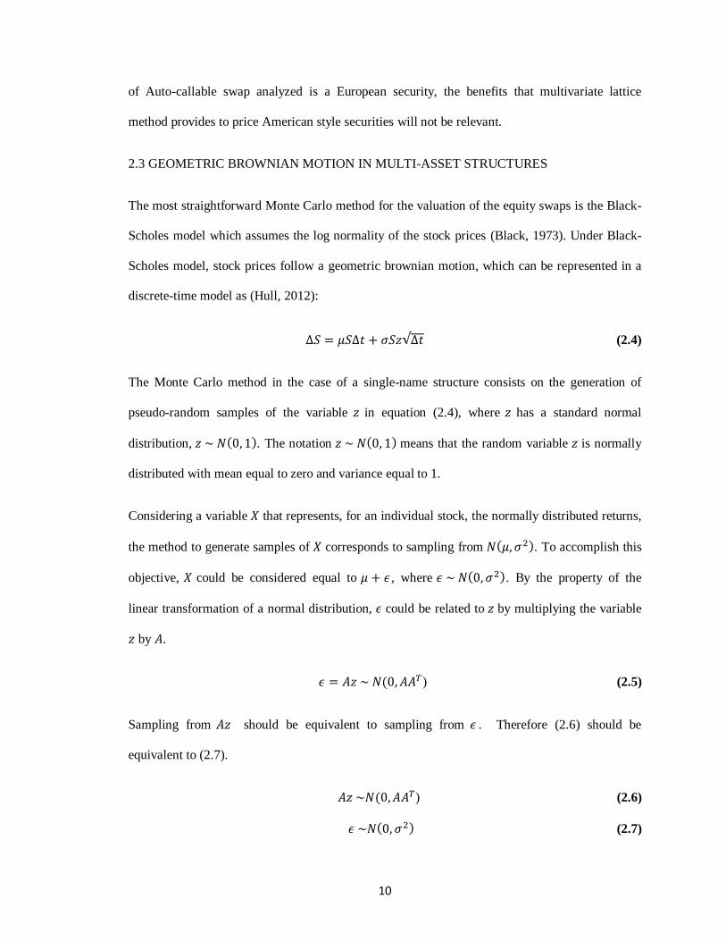
The most straightforward Monte Carlo method for the valuation of the equity swaps is the Black-
Scholes model which assumes the log normality of the stock prices (Black, 1973). Under Black-
Scholes model, stock prices follow a geometric brownian motion, which can be represented in a
discrete-time model as (Hull, 2012):
√ (2.4)
The Monte Carlo method in the case of a single-name structure consists on the generation of
pseudo-random samples of the variable in equation (2.4), where has a standard normal
distribution, ( ). The notation ( ) means that the random variable is normally
distributed with mean equal to zero and variance equal to 1.
Considering a variable that represents, for an individual stock, the normally distributed returns,
the method to generate samples of corresponds to sampling from ( ). To accomplish this
objective, could be considered equal to , where ( ). By the property of the
linear transformation of a normal distribution, could be related to by multiplying the variable
by .
( ) (2.5)
Sampling from should be equivalent to sampling from . Therefore (2.6) should be
equivalent to (2.7).
( ) (2.6)
( ) (2.7)
11
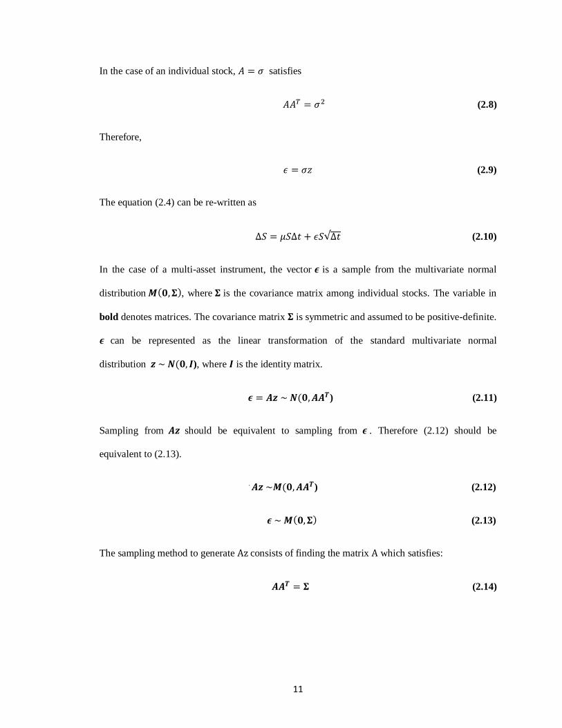
In the case of an individual stock, satisfies
(2.8)
Therefore,
(2.9)
The equation (2.4) can be re-written as
√ (2.10)
In the case of a multi-asset instrument, the vector is a sample from the multivariate normal
distribution ( ), where is the covariance matrix among individual stocks. The variable in
bold denotes matrices. The covariance matrix is symmetric and assumed to be positive-definite.
can be represented as the linear transformation of the standard multivariate normal
distribution ( ), where is the identity matrix.
( ) (2.11)
Sampling from should be equivalent to sampling from . Therefore (2.12) should be
equivalent to (2.13).
. ( ) (2.12)
( ) (2.13)
The sampling method to generate consists of finding the matrix which satisfies:
(2.14)

12
The Cholesky factorization described in Glasserman (2003) uses a lower triangular matrix of j
order which satisfies (2.14), for a covariance matrix symmetric and positive-definite. Below is
an example of for the case of 3 stocks in the basket.
[
] (2.15)
The multiplication of for its transpose gives
[
] (2.16)
The equation (2.14) is finally solved by making (2.16) equal to the covariance matrix and
resolving an algorithm that starts by finding and proceeds to the remaining elements of . For
instance and can be obtained by solving:
Matrix in this example can be expressed as:
[
]
[
√ (
)
(
)
√ (
)
√
(
)
(
(
)
√ (
)
)
]
(2.17)
Using (2.17) in (2.11), is given by:
[
] [
] [
] = [
] (2.18)
13
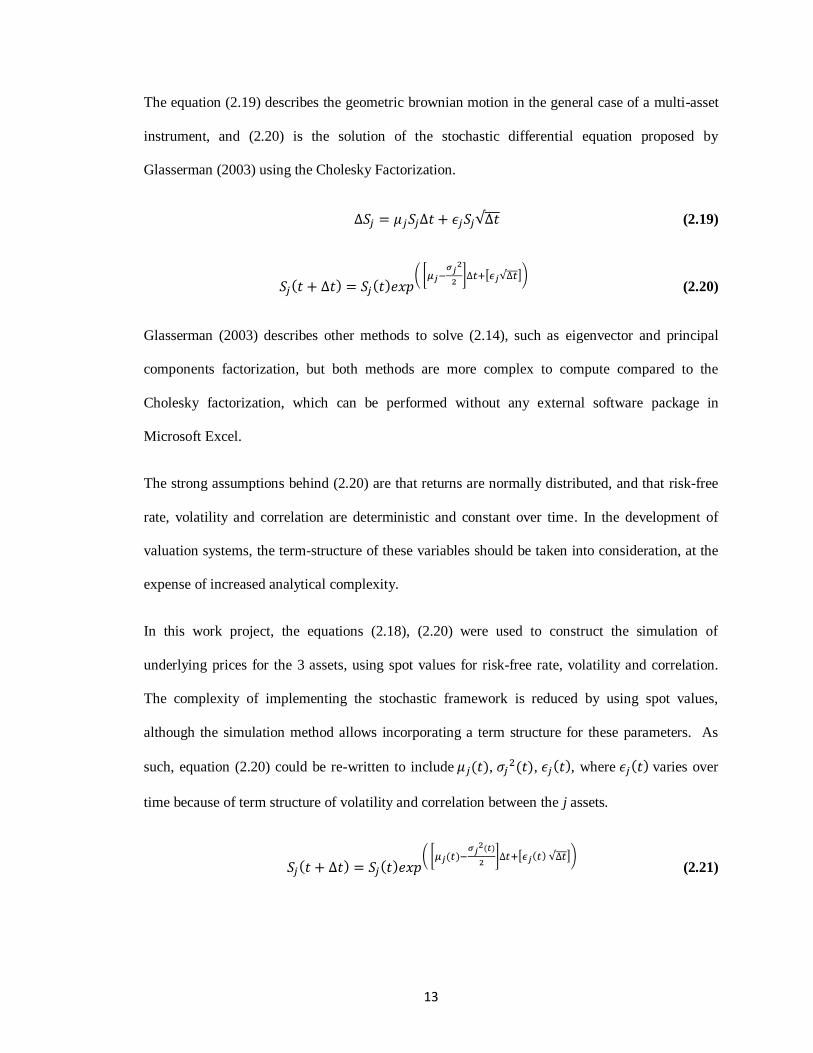
The equation (2.19) describes the geometric brownian motion in the general case of a multi-asset
instrument, and (2.20) is the solution of the stochastic differential equation proposed by
Glasserman (2003) using the Cholesky Factorization.
√ (2.19)
( ) ( ) ( [
] [ √ ])
(2.20)
Glasserman (2003) describes other methods to solve (2.14), such as eigenvector and principal
components factorization, but both methods are more complex to compute compared to the
Cholesky factorization, which can be performed without any external software package in
Microsoft Excel.
The strong assumptions behind (2.20) are that returns are normally distributed, and that risk-free
rate, volatility and correlation are deterministic and constant over time. In the development of
valuation systems, the term-structure of these variables should be taken into consideration, at the
expense of increased analytical complexity.
In this work project, the equations (2.18), (2.20) were used to construct the simulation of
underlying prices for the 3 assets, using spot values for risk-free rate, volatility and correlation.
The complexity of implementing the stochastic framework is reduced by using spot values,
although the simulation method allows incorporating a term structure for these parameters. As
such, equation (2.20) could be re-written to include ( ), ( ), ( ), where ( ) varies over
time because of term structure of volatility and correlation between the j assets.
( ) ( ) ( [ ( )
( )
] [ ( ) √ ])
(2.21)
14
A more complex way of treating volatility is to consider a volatility surface (Andersen, 1998),
where variance ( ( )) could be a deterministic function of time and price ( ). But the
strict implementation of this method would require the solution of Cholesky Factorization (2.17)
for every single point in the simulation, which would require computational resources beyond the
scope of a simple valuation method.
2.4 GENERATION OF RANDOM SAMPLES
The Monte Carlo method consists on simulating prices for the stocks, inside the structure, using
equation (2.20) and (2.18). The first step is to generate random samples for the vector , which is
normally distributed.
According to Glasserman (2003), pseudo-random samples are obtained applying the inverse
cumulative normal distribution over a random sample of the uniform distribution ( ).
denotes the inverse cumulative normal distribution.
(2.22)
Glasserman (2003) argues that modern pseudo-random generators are sufficiently good at
replicating genuine randomness.
There are other methods called Quasi-Monte Carlo methods, or low-discrepancy sequences,
which are alternatives to the pseudo-random generation, where samples are drawn from the
uniform distribution in a way that minimizes the relative dispersion among samples. As a result,
the sample space of the uniform distribution ( ) is covered with evenly dispersed
samples (Glasserman, 2003).
Despite the name, Quasi-Monte Carlo methods are completely deterministic, and Corwin (1996)
shows that Quasi-Monte Carlo is a more efficient numerical method to price securities than a
standard Monte Carlo, because the valuation results converges more rapidly as the number of

15
simulated scenarios increases. But the implementation of a low-discrepancy method in a simple
valuation model is far more complex than a pseudo-random method, as it requires special
libraries of software.
2.5 PRICING OF EQUITY DERIVATIVES WITH MONTE CARLO
The pricing of derivative securities with Monte Carlo uses the risk-neutral dynamics of the
simulated paths for the price of the underlying asset. The equation (2.20) is used to calculate the
paths for the prices of the j stocks, based on the samples generated through (2.22) and
transformed using (2.18). The payoff of the derivative is calculated for each path, and the
expected value of the discounted payoffs at risk-free rate provides the estimate for the price of the
security (Glasserman, 2003).
The pricing of the Worst-of auto-callable swap will be described in the following section in
greater detail, but it consists on generating paths for the prices of the underlyings in each
observation date and taking the average of the present value payoff of each path. Each simulated
path may or may not assume several cash flows until maturity, depending on the trigger of the
coupon payments before and at maturity and the payoff of the option at maturity.
2.6 VARIANCE AND BIAS OF THE MONTE CARLO METHOD
The efficiency of a Monte Carlo simulation is defined by the accuracy and precision of the
simulation output. Glasserman (2003) uses the central limit theorem to show that the error
between the unbiased expected value from a Monte Carlo simulation and the true value tends
to a normal distribution (
) as the number of simulated scenarios n increases, provided that
the simulation output is independently and identically distributed.

16
(
) (2.23)
is the variance calculated from the simulation output.
Therefore, it should be possible to reduce the variance of an unbiased simulation output by
increasing and consequently the computational time. But as Glasserman (2003) argues,
increasing computational time is not worthwhile if the simulation output converges to an
incorrect value – an error caused by the simulation discretization bias and other types of biases.
One of the sources of bias in the valuation method proposed for the Worst-of auto-callable swap
is the discretization error. The valuation method calculates the prices of the stocks only at the 12
observation dates, consequently in equation (2.20) is equal to 21 trading days. This choice of
is a matter of reducing computational time and complexity, allowing the method to be
implemented in a standard tool such as Microsoft Excel.
17
CHAPTER III
METHODOLOGY
The hypothesis in the first research question is that the simulation method is a feasible solution
for pricing Worst-of auto-callable swaps. The testing of this hypothesis requires building the
simulation method per se and analyzing the dispersion and bias of the results as well the
computational time needed.
The hypothesis in the second research question is that a simple valuation method is a cost-
effective solution as a benchmark tool for the deployment of complex valuation systems. To test
this hypothesis, valuation data collected from a black-box valuation system deployed in a
financial institution were compared to the prices obtained in the method developed in this thesis.
A linear regression analysis was used to determine if the proposed method is relevant to explain
the dispersion on the valuation data collected.
This Chapter is organized in the following sequence: in the first section, it is described the
proposed Monte Carlo Valuation for the Worst-of auto-callable swap and the model embedded in
the “black-box” valuation system; in the second section, the procedures used in the data
collection of the valuation samples are explained; in the third section, it is described the
experiment designed to test hypothesis ; in the fourth section, it is described the experiment
designed to test hypothesis .
3.1 MONTE CARLO VALUATION OF WORST-OF AUTO-CALLABLE SWAP
The swap analyzed in this thesis was contingent to 3 underlying stocks and had 12 observation
dates including maturity. The valuation of the swap was based on a discrete method which
simulated, for every observation date , prices for the 3 assets {
. Considering, for

18
a particular simulation run, that scenarios were simulated in every observation date for all
assets, 12 triplets of prices were obtained. The general representation of a triplet for scenario
in observation date is
[
] (3.1)
where i = 1 to 12 and n = 1 to N.
The stock prices of the triplets were obtained from the multi-asset geometric brownian motion
model (2.20). The model was calibrated using spot values for risk-free rate, volatility and
correlation, and was calculated using the Cholesky Factorization in (2.18) and the pseudo-
random numbers of in (2.22). Microsoft Excel was used to implement the model and the
simulation.
The payoff for a triplet was calculated using the coupon formula (2.1) and, for triplets at maturity,
the payoff also incorporated the redemption given by formula (2.2).
( )
( ) - { ( ) (3.2)
The expected payoff for each observation date is the average payoff of all N triplets simulated for
that observation date,
[ ( )] (3.3)
where n = 1 to N.
The final present value of the structured leg is the sum of the discounted expected payoffs of all
observation dates.
∑ (3.4)
19
The “black-box” valuation system, used as benchmark in this thesis, implements a Quasi-Monte
Carlo simulation for generating prices for the underlyings in the basket. The simulation
implements a multi-asset geometric brownian motion model, using an Eigenvector factorization
of the covariance matrix and Sobol sequences (low-discrepancy sequences) to feed the
simulation. Moreover, the system is able to simulate daily prices for the underlyings, reducing the
discretization effects in the output. These characteristics should allow for better precision and
better accuracy of the valuation output when compared to less sophisticated systems.
One potential source of issues in “black-box” valuation is the customization of the payoff
calculation for each type of structure in the portfolio of the financial institution. The financial
engineer responsible for the system customizes each structure inside the system by implementing
a script, written typically in proprietary programming language. This script controls how payoffs
are triggered and calculated during the simulation, affecting directly the output of the valuation.
Because of human intervention and complexity of the structures, the script can be a major source
of operational errors in deployed “black-box” systems.
3.2 DATA COLLECTION PROCEDURES
The output of the simulation collected in the analysis represents the estimation of the value of
structured leg of the swap, at the valuation date, calculated using (3.4). The data points for the
analysis were collected from a batch of predefined number of runs with different number of
scenarios simulated. The output of each run represented a data point, and the runs were executed
using different samples of , pseudo-randomly selected every new run using (2.22). The standard
deviation and average of the data point samples were calculated for each batch of runs. The
results displayed in the thesis represent the average and standard deviations of the structured leg
as a percentage of the notional of the swap.
20
3.3 EXPERIMENTS TO TEST VARIANCE AND BIAS
The hypothesis required an experiment to test if variance and bias could be reduced
increasing the number of simulated scenarios. Computational time of the method should be in
interval of minutes, as opposed to hours, for the method to be of practical use. Therefore,
hypothesis will be accepted if variance and bias can be controlled using a reasonable amount
of computational time.
The experiment consisted on increasing the number of runs and scenarios and computing the
impact on the variance of the simulation output. The expected result from the experiment was that
variance decreased as either the number of simulated scenarios increased or the number of runs
per batch increased.
A second experiment was built to analyze specifically the discretization bias caused by
equal to 21 trading days in (2.20). In the experiment, was reduced to 10 trading days in one
population and kept at 21 days in another population. The expected result from the experiment
was that the population with =10 days had a faster convergence and reduced bias compared
with the population with =21 days. For this experiment, identical samples of were used in
both populations in order to measure only the variance caused by the discretization effect. The
only difference in this respect was that with =10 days additional samples of were required in
the intermediate sampling points which were not part of the population with =21 days.
3.4 BENCHMARK ANALYSIS
The hypothesis required an experiment to compare the proposed method with a “black-box”
valuation method. This experiment intended to assess the magnitude of errors caused by all
differences between the methods used. These differences include discretization, calibration

21
(volatility, risk-free rate and correlation), but more importantly differences in the stochastic
model.
The experiment built consisted on getting as many diverse valuation data points as possible,
from one “black-box” system, and comparing with the corresponding result from the Monte Carlo
method. The “black-box” system used live market inputs to calibrate the valuation (correlation,
risk-free rate, spot prices and volatility), and these inputs were replicated identically to calibrate
the model.
The data collection happened throughout the summer of 2011, when a significant movement of
the market occurred, allowing a comparison over a wide range of spot prices, volatilities and
valuation prices. In this experiment, the output value from the method was the average of 10
simulation runs with 10.000 scenarios. A linear regression analysis using SPSS was performed
upon the experimental results to determine if the Monte Carlo method is statically significant to
predict the results of the “black-box” system. The valuation results were expressed as percentages
of the notional of the swap contract.
22
CHAPTER IV
RESULTS
This Chapter is organized in the following sequence: in the first section, it is showed the results of
experiment about the reduction of the variance of the simulation output; in the second
section, the results of experiment about the effects of discretization bias; in the third
section, it is analyzed the results of experiment about the fit of the numerical model to the
one “black-box” valuation system.
4.1 VARIANCE REDUCTION
The model created in Microsoft Excel performed well up to 10.000 simulated scenarios, with
computational time of 1 second for every run. For every scenario simulated, the model needs to
calculate 278 internal variables, which for a run with 10.000 scenarios yields to at least 2,7
million calculations in total. With 20.000 scenarios, Excel started to crash and function
abnormally because of its large memory consumption above 1GB, making almost impossible to
run the simulation in a Windows 7 machine with 4GB of memory.
The first result of experiment is the comparison of standard deviation of the data points of
(3.4) among different composition of batches: with different number of runs and different number
of scenarios simulated per run. All other inputs and characteristics of the swap were kept
constant.
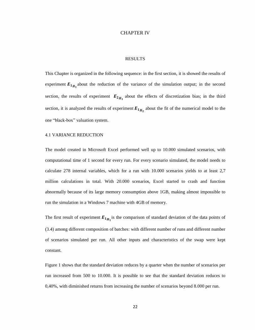
Figure 1 shows that the standard deviation reduces by a quarter when the number of scenarios per
run increased from 500 to 10.000. It is possible to see that the standard deviation reduces to
0,40%, with diminished returns from increasing the number of scenarios beyond 8.000 per run.
23
Another result is that the number of runs per batch has little influence on the reduction of
variance when a large number of scenarios per run is already used. On the other hand, for a lower
number of scenarios, batches as large as 50 runs deviates by at least 10 basis points from batches
with more than 250 runs.
Figure 1: Effects of different batch compositions on the standard deviation of the output
These findings have important implications for the computation time of the model: a batch
composed of 10 runs with 10.000 scenarios simulated will take about 10 seconds to execute
whereas a batch composed of 1.000 runs with 10.000 scenarios simulated will execute in 1.000
seconds, and yet no significant reduction in dispersion will be achieved in the latter case.

24
The results of experiment allow concluding that it is feasible to construct such a method, in
which variance can be controlled within a reasonable interval of computational time.
4.2 EFFECT OF DISCRETIZATION BIAS
In order to isolate and measure the effects of the discretization bias of the model, experiment
was conducted using a control population with =21 days (monthly sampling) and a test
population with =10 days (bi-weekly sampling). The pseudo-random samples for both
populations were kept the same for all runs, with the consideration that additional samples of
were required in the test population. All other characteristics of the swap were kept equal.
If there were no discretization bias, both populations were expected to provide the same results or
very similar results regardless of the number of simulated scenarios used, but in fact the results
showed in Figure 2 indicate that reducing discretization creates variation on the expected value of
the test population compared to the one of the control population. Moreover, this variation
reduces as the number of simulated scenarios is increased.
Figure 2: %error between valuations with monthly and with bi-weekly samplings

25
In Figure 2, the monthly data series represents the expected values measured by the model for the
control population =21 days, whereas the bi-weekly data series represents those measured for
the test population =10 days. The two data series converge as the number of simulated
scenarios is increased, demonstrating the possibility of reducing the discretization bias by
increasing the size of the simulation.
The data series that measures the was calculated by:
|
|
The reduction in the of the expected value in larger simulations follows the same pattern
of reduction as the standard deviation in Figure 2, demonstrating the possibility of controlling and
reducing both bias and variance in the simulation output.
The results from experiments and
confirms hypothesis that it is feasible to
construct a Monte Carlo method that allows to reduce both variance and discretization error to
levels below 1% of the notional. The recommended simulation setting is to use at least 10
simulations runs with 10.000 independently simulated scenarios.
4.3 BENCHMARK RESULTS
The experiment was conducted with one swap contract denominated in dollars containing 3
stocks also denominated in dollars. A regression analysis was performed to determine if the
valuation provided by the Monte Carlo method, obtained from 10 runs with 10.000 simulated
scenarios, could be used as a predictor for the valuation of one particular “black-box” valuation
system.

26
The system used in this experiment had been implemented in a financial institution that used it to
value Worst-of auto-callable swaps. The inputs used for the system calibration were copied to
calibrate the Monte Carlo method, and the system results were compared with the expected value
of the Monte Carlo method. Table 1 shows the 16 data points collected for the regression
analysis. The values were presented as percentages of the notional of the swap contract.
(X) Value (model)
% Notional
(Y) Value (System)
% Notional
(W ) = (X)-(Y) Error
%Notional
-1,9% -0,7% -1,2%
-1,7% -0,7% -1,0%
1,1% 0,2% 1,0%
1,1% 0,0% 1,0%
-0,3% -0,7% 0,4%
-15,4% -11,2% -4,2%
-32,5% -32,9% 0,4%
-28,1% -28,2% 0,2%
-24,8% -22,6% -2,2%
-27,4% -26,5% -0,9%
-8,4% -10,6% 2,2%
-17,9% -18,4% 0,5%
-20,9% -21,8% 0,9%
-20,8% -21,3% 0,4%
-18,8% -19,1% 0,3%
-40,1% -37,5% -2,6%
Table 1: Data points collected from the Valuation system and the Monte Carlo method
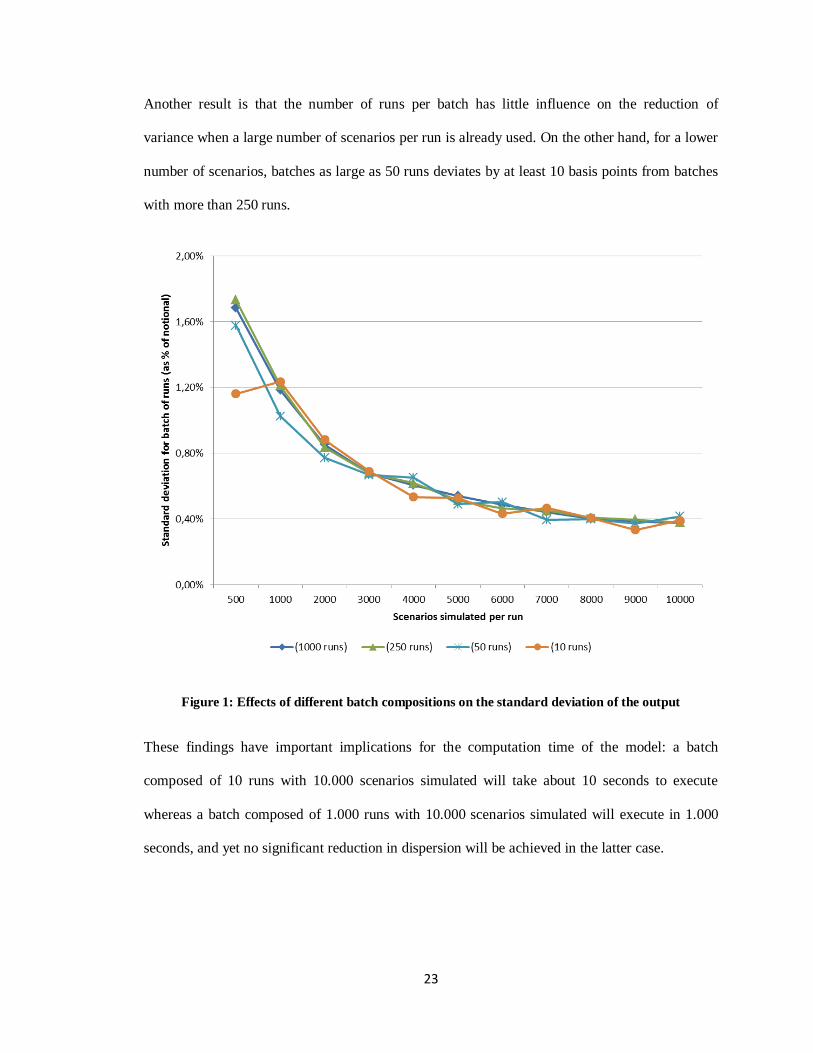
The scatter-plot in Figure 3 suggests that there is an important correlation between the valuation
of the model and the valuation of the system. The regression analysis in Table 2 indicates that the
correlation between the model and the system is statically significant (p equals 0,000) with a beta
of 0,991. Consequently, it is possible to reject the null hypothesis that the two valuations methods
are not correlated.
27
Figure 3: Scatter-plot of the System valuation as a function of the Model valuation
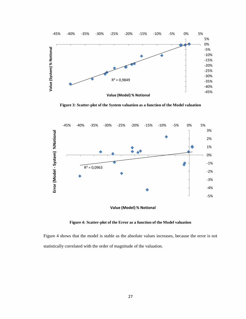
Figure 4: Scatter-plot of the Error as a function of the Model valuation
Figure 4 shows that the model is stable as the absolute values increases, because the error is not
statistically correlated with the order of magnitude of the valuation.
R² = 0,9849
-45%
-40%
-35%
-30%
-25%
-20%
-15%
-10%
-5%
0%
5%
-45% -40% -35% -30% -25% -20% -15% -10% -5% 0% 5%
Va
lue
(Sys
tem
) % N
oti
on
al
Value (Model) % Notional
R² = 0,0963
-5%
-4%
-3%
-2%
-1%
0%
1%
2%
3%
-45% -40% -35% -30% -25% -20% -15% -10% -5% 0% 5%
Erro
r (M
od
el -
Sys
tem
) %
No
tio
nal
Value (Model) % Notional

28
Model Summaryb
Model R R Square Adjusted R Square Std. Error of the Estimate
1 ,991a ,982 ,981 ,0160886
a. Predictors: (Constant), Value_Mode
b. Dependent Variable: Value_System
ANOVAb
Model Sum of Squares df Mean Square F Sig.
1 Regression ,186 1 ,186 719,282 ,000a
Residual ,003 13 ,000
Total ,190 14
a. Predictors: (Constant), Value_Mode
b. Dependent Variable: Value_System
Coefficientsa
Model
Unstandardized Coefficients
Standardized
Coefficients
t Sig. B Std. Error Beta
1 (Constant) -,002 ,007 -,227 ,824
Value_Mode ,979 ,036 ,991 26,819 ,000
a. Dependent Variable: Value_System
Table 2: SPSS regression analysis results of the System valuation and Model valuation
The alpha of regression analysis in Table 2 is not statistically significant, providing an indication
that there is not a bias in the results of one method when compared with the other. But the
average alpha of -0,2% is close to the order of magnitude of the typical profit obtained by
financial institutions on this operation, indicating a possible limitation to the usage of the Monte
Carlo method as a standalone valuation method.
One possible inference from the results above is that there is not a significant difference in the
stochastic model and the random simulation between the two methods. In fact, it is known that
29
the valuation system implements a multi-asset Black Scholes model using an Eigenvector
factorization and Sobol sequences (low-discrepancy sequences) to feed the simulation. In theory,
these methodologies are similar to the Cholesky factorization and pseudo-random numbers used
in the Monte Carlo method. Therefore, results were expected to be similar provided that the same
inputs were used.
This experiment confirms hypothesis that the Monte Carlo method is a cost-effective
benchmark tool for the valuation system under study. In the example of new structures or
modifications in the structure definition of the Worst-of auto-callable, the financial institution can
use this method to assess the correctness of the results provided by the valuation system.

30
CHAPTER V
CONCLUSION
This thesis started by discussing the difficulty that financial institutions have assessing the quality
of the output provided by “black-box” systems used in the valuation of complex financial
securities. Because a wide range of complex securities cannot be value in closed-form, it is
important that alternative valuation methods become available.
A Monte Carlo method was constructed to illustrate the case of valuing a Worst-of Auto-callable
swap. The Worst-of Auto-callable is an equity swap with a basket of underlying stocks and with
an embedded barrier option that provides a payoff in terms of the worst performing stock at
maturity. The exotic features of the instrument prevent its valuation in closed-form.
The thesis proposed a method based on a geometric brownian motion model that generated the
stock prices of as many underlyings as needed, taking into consideration the covariance among
them. The simulation of scenarios occurred generating pseudo-random numbers that fed the
stochastic model. The expected value of the structure was obtained from the probability-weighted
average of the payoff of each scenario simulated.
The method created was based on the theoretical framework researched and the term-sheet
specification of one Worst-of auto-callable swap with 3 underlying stocks. The access inside the
“black-box” system was not required in the creation of the method.
Microsoft Excel was chosen for the implementation, because the method needed to be fast, easy
to replicate and modify in order for it to be of practical use. Although Excel is not a robust tool
for large simulation with hundreds of thousands of scenarios simulated at once, it provided an

31
unmatched flexibility to the implementation. In Excel, the Cholesky factorization and pseudo-
random number generation were the alternative methods used to avoid expensive and additional
software packages.
Based on the two research questions raised, three experiments were built to analyze the method
and determine if it were a valid alternative to assess the quality of “black-box” valuation systems.
The results from the first experiment demonstrated that a pseudo-random method generates
variance in the valuation output that can be controlled increasing the number of scenarios
simulated or the number of simulation runs. In the case studied, the standard deviation using
10.000 scenarios was one fourth of the one using 500 scenarios, or 0,4% of the notional.
The second experiment showed that discretization bias is present on such stochastic models that
do not discriminate time intervals as smaller as possible. But it was demonstrated that the bias
effect was also reduced with an increase in the number of simulated scenarios.
The third experiment compared the results of the method with one particular valuation system
implemented in a financial institution, which trades Worst-of auto-callable swaps. The results of
the regression analysis demonstrated that the valuations of the methods were highly correlated,
encouraging the use of the method as a benchmark tool for “black-box” valuation systems.
Moreover, it became clear that although it is possible to control the intrinsic error of the model
caused by variance and bias, the size of the error is in the same order of magnitude of the profit
margin for the financial institution. Therefore, the method proposed could best serve as a cost-
effective benchmark tool on the deployment of new products or valuation systems rather than as a
standalone valuation tool.
Future enhancements of the method could include implementing low-discrepancy sequences or
other type of factorization. But the major gap in the current implementation of the model is to not

32
consider a volatility surface. As mentioned before, a volatility surface would require the
Cholesky factorization to be computed for every node simulated – approximately 2 million
additional computations in a structure with 3 assets. Microsoft Excel lacks robustness to
implement this enhancement, but the volatility surface could be implemented with a higher level
of discretization to meet Excel limitations. Further research could be conducted to investigate the
impact on valuation effectiveness of implementing such volatility surface.
The implementation in Excel allows for easy modifications in the number of assets and in the
calculation of the payoffs. The method described in this thesis can be applied, without major
modifications, to single name auto-callable swaps with barrier options or to similar Worst-of
structures, such as Worst-of reverse convertibles. For structures that have accrual mechanisms
that require daily monitoring of stock prices, the method could be used, but Excel would need to
be replaced by a more robust simulation tool.

33
REFERENCES
Andersen, L.B.G.; Brotherton-Ratcliffe, R. The equity option volatility smile: an implicit finite-
difference approach, Journal of Computational Finance, 1998, 2, p. 5-35.
Black, F.; Scholes, M. The Pricing of Options and Corporate Liabilities, Journal of Political
Economy, 1973, 81, p.637-659
Boyle, P.; Evnine, J.; Gibbs, S. Numerical evaluation of multivariate contingent claims, Review
of Financial Studies, 1989, 2, p.241-250
Boyle, P.; Broadie, M; Glasserman, P. Monte Carlo methods for security pricing, Journal of
Economic Dynamics and Control, 1997, 21, p.1267-1321
Broadie, M; Glasserman, P. Pricing American – style securities using simulation, Journal of
Economic Dynamics and Control, 1997, 21, p.1323-1352Corwin, J.; Boyle, P.; Tan, K. Quasi-
Monte Carlo Methods in Numerical Finance, Management Science, 1996, 42, p. 926-938
Fries, C.; Joshi, M. Conditional Analytic Monte-Carlo Pricing Scheme of Auto-Callable
Products, 2008
Glasserman, P. Monte Carlo Methods in Financial Engineering (Stochastic Modeling and
Applied Probability), Springer, 2003, p.39, 104
Johnson, H. Options on the maximum or minimum of several assets, Journal of Financial and
Quantitative Analysis, 1987, 22, p.227-823.
Haug, E.G. The Complete Guide to Option Pricing Formulas, McGraw-Hill, 2006

34
Hull, J.C. Options, Futures, and Other Derivative Securities, Pearson Education, 2012, p.287,
582, 587-588
Lee, J. Index-linked products and downside protection drive investor interest in Asia, Structured
Products, 2011, 12
Osseiran, A.; Bouzoubaa, M. Exotic Options and Hybrids, John Wiley & Sons, 2011
Wong, J. Asia Risk wealth rankings 2011, Asia Risk, 2011, 11

Top Related