


Languages
Pages
Legal


THE APPLICATION OFDIFFERENTIAL PULSE ANODIC
STRIPPING VOLTAMMETRY FORTHE DETERMINATION OF COPPER,
LEAD, ZINC AND CADMIUM INAIRBORNE PARTICULATE
MATTER.
MOHAMMED NAZEEM JAHED
Research dissertation submitted in fulfilment of the requirements for the
MASTERS DIPLOMA IN TECHNOLOGY (Chemistry)
in the Department of Physical Sciences at the
PENINSUIA TECHNIKON.
Date of Submission: January 1995
Promoter: Professor A M CROUCH

ACKNOWLEDGEMENTS
I would like to express my sincere thanks to:
Prof. A.M. Crouch for constant encouragement, help and invaluable advice
throughout this study.
Miss P. Robertson for assisting with the analysis.
Dr. W. T. Mabusela for proof reading this work.
Mrs A. Van Niekerk for typing this thesis.
Mr. B. Solomons and Mr. J. Peterse for their technical support.
Mr. J.H. De Bruyn and Mr. C.H. Le Roux for their technical support.
ESCOM for their financial support and for expressing an interest in this project.

LIST OF CONTENTS
Page
CHAPTER 1 Introduction
1.1 Historical Bacground of Polarography and Voltammetry 2
1.2 Polarography and Voltammetry 5
1.2.1 Differential Pulse Polarography 6
1.2.2 Anodic Stripping Voltammetry 6
1.3. Electrochemical Processes in Polarography and Voltammetry 8
1.3.1 Faradaic and Non-Faradaic Processes 8
1.3.2. Mass Transfer Processes 9
1.3.3 Charging Current 10
1.3.4 Diffusion Current 10
1.4 General Practical Considerations 12
1.5.0 Sample Collection 15
1.5.1 Particulate Pollutants 15
1.5.2 Filtration 16
1.6. Sample Preparation Methods 19
1.6.1 Dry Ashing Method 19
1.6.2 Dry Ashing with Additives 20
1.6.3 Oxidation with HN03 and H2S04 20
1.6.4 Oxidation with excited Oxygen 21
1.6.5 Destruction in a closed vessel at high pressure 22
ii

CHAYrER 2 :- Experimental
2.0. Instrumentation
2.1. Instrumental Parameters
2.2. Reagents and Equipment
2.3. Purification of Water
2.3.1 High Purity Water (HPW)
2.3.2 Ultra High Purity Water (UHPW)
2.3.3 Cleansing of Glassware
2.4. Standard Solutions
2.4.1 Ammonia-Ammonium Chloride Buffer Solution
2.4.2 Nitric Acid Solution (6 Molar)
2.4.3 Electrolyte Solution (0.1 Molar HCl)
2.5. Sample Collection
2.6 Digestion of Samples
2.6.1 Digestion Method 1
2.6.2. Digestion Method 2
2.7. Sample Analysis
2.8 Quantitation
Page
23
24
25
26
26
26
26
27
27
27
27
28
29
29
29
30
31
III

CHAPTER 3 :-Results and Discussion
Page
3.0. Contamination 32
3.l. Recovery studies: Digestion Method 35
3.2. Digestion Method 1: Applied to Air Samples 42
3.3. Recovery studies: Digestion Method 2 42
3.4. Digestion Method 2: Applied to Air Samples 46
3.5. Concentration Variations of Metallic Pollutants 52
3.6. Monthly Metal Averages 61
3.7. Meteorological Data for 1992 65
3.8. Meteorological Factors Influencing Air Pollution 73
CHAPTER 4.:- Conclusions
APPENDIX
REFERENCES
76
77
85
iv

DPASV
ASV
DME
a.u.
%RSD
LIST OF ABBREVIATIONS
Differential Pulse Anodic Stripping Voltammetry
Anodic Stripping Voltammetry
Dropping Mercury Electrode
arbitrary units
Percentage Relative Standard Deviation
v

SUMMARY
An analytical method using Differential Pulse Anodic Stripping Voltammetry was
developed for determining trace quantities of Cu, Pb, Cd and Zn in airborne
particulate matter. The levels of the metallic pollutants were evaluated against
meteorological data.
Instrumental parameters and sample processing were optimised for determining
the metals in the concentration range 1 to 40 ~g/l with a percentage relative
standard deviation (%RSD) less than 10%.
Airborne particulate matter was decomposed by heating in a mixture of
Hydrochloric and Sulphuric acids. Recovery studies were used to evaluate the
digestion procedure, in the absence of a suitable reference material. The
percentage recovery for the metals were between 95% and 100%. A total of 77
air samples were collected from January to December 1992, on the campus of the
Peninsula Technikon. The samples were collected over 24 hour periods by
filtration at a sampling rate of 20 liters per minute. The total average concentration
for the metals was 25.3 ~g1m3. No Cd was detected in any of the samples.
1

CHAPTERl
INTRODUCTION
1.1 HISTORICAL BACKGROUND OF VOLTAMMETRY
In the early 1920's J. Heyrovsky developed the technique of Polarography, from
which the field of Voltammetry was developed. Whilst attempting to measure the
amount of Copper plated onto a Platinum electrode Zbinden in 1931, found it
extremely difficult to weigh accurately the small amount of Copper which plated
out. He however, made a quantitative determination by measuring the amount of
current consumed during the electrochemical stripping of Copper from the
Platinum electrode. This was thus the birth of the concept of Stripping Analysis.
With the development of the Hanging Mercury Drop Electrode (HMDE) by
W.Kemula in the early 1950's, Kemula and other workers emphasised the
sensitivity attained with this technique, since Cadmium could then be determined
below the parts per billion range. The rapid advancements made in electronics
during the 1960's, coupled to a better understanding of the theoretical principles of
stripping analysis, spurred the manufacture of low cost instruments and as a
consequence, newer, more sensitive and inore reliable procedures were developed
in the 1970's, amongst which is Differential Pulse Anodic Stripping Voltamrnetry
(DPASV).
2

The last ten to fifteen years were marked by the introduction of computer
operated instruments which generated automated, rapid and reliable results and
further broadened the scope of Stripping analysis [1].
The low cost of instruments, the high sensitivity of the technique and the capability
of determining more than one metal in a single sample solution, prompted
scientists to apply the Anodic Stripping Voltammetry (ASY) technique to many
diverse areas of analysis. Typical examples include the determination of trace
quantities of metals such as Cu, Pb, Cd, Zn and Bi in ground and spring water [2],
rain water [3,4], natural waters and atmospheric precipitation [5]. These metals
have also been determined in clinical samples, namely blood [6], urine [7] and in
various biological materials [8,9,10,11,12].
The presence of metals in suspended airborne metals which have been
predominantly determined by Atomic Absorption spectroscopy [13,14,15] has also
been successfully determined by Anodic Stripping Voltammetry (ASY) [16,17].
Since heavy metals are not biodegradable, they are retained indefinitely in the
ecosystem and are considered to be the most harmful of pollutants. Some twenty
years ago Colovos and co - workers developed an Anodic Stripping Voltammetric
technique for determining Cd, Cu, Pb and Zn in airborne particulate matter. This
procedure involved collecting the particulate matter by filtration onto a membrane
filter (0.22 f!m) and decomposing the 'sample by low-temperature ashing in a
bomb. The results obtained were comparable to those obtained with Atomic
Absorption Spectroscopy [17]. Harrison and Winchester successfully used
Anodic Stripping Voltammetry for air pollution control studies [16], whilst other
workers monitored air samples adjacent to highways where the suspended
particulate matter comprised mainly of fuel combustion products [1]
3

Modem life demands of the Analyst to be able to determine trace amounts of
metals in complicated sample matrices. However, trace metal analysis requires the
successful contention in four analytical aspects, before valid results can be
obtained. These are:
1. Achieving sufficient sensitivity of the method Le. a sufficiently high signal to
noise ratio. With the advent of computer operated analytical instruments and solid
state electronics, analytical techniques such as Inductively Coupled Plasma Atomic
Emission Speetrometry [18] and Flameless Atomic Absorption Spectrometry [15]
are capable of sensitivities in the parts per billion range.
2. Achieving selectivity required to determine trace components of the system
in the presence of other substances at several orders of magnitude higher; this
problem is in many cases not solvable without the use of preliminary separation
methods. The use of chelating agents for example Dithiazone [19], and
Dimethylglyoxime [20], or in the form of ion-exchange resins [21], and the
technique of liquid-liquid extraction [22] is often helpful in the separation and pre
concentration of the metallic species.
3. Obtaining sufficiently pure chemicals so that the influence on the
experimental results due to contamination is minimized.
4. Acquiring a skill for working with extremely dilute solutions, since losses of
the analyte may readily occur through, for example, adsorption onto the walls of
the vessels, hydrolysis, etc. [23].
4

1.2 POLAROGRAPHY AND VOLTAMMETRY
In Voltammetry a linearly increasing voltage is applied to the cell and the current
generated is plotted as a function of the applied voltage. The current - voltage
curves are called Voltammograms. The cell consists of:
1. an electrolyte solution containing the analyte,
2. a reference electrode and
3. an indicator electrode.
When the indicator electrode is a Dropping Mercury Electrode (DME) the
technique is known as Polarography and the current-voltage curves are known as
Polarograms. The voltage applied to the cell is measured relative to a standard
reference electrode e.g. Saturated Calomel Electrode (SCE) [24].
The Dropping Mercury Electrode consists of a glass capillary attached to a
mercury reservoir. Drops of mercury fall from the capillary orifice at a constant
rate of between 5-20 drops per minute. This technique is often called
"Conventional" or "DC" (direct-current) polarography. DC polarography has a
detection limit between 1 and 5 x 10⁻⁶ M, whereas other polarographic
techniques, such as Differential Pulse Polarography, offer a lower detection limit,
namely 1 x 10⁻⁸ M [24].
5
1.2.1 DIFFERENTIAL PULSE POLAROGRAPHY
In Differential Pulse Polarography, a linearly increasing direct current voltage is
applied to the cell, and as the mercury drop nears the end of its life a pulse with
amplitude of 50 mV is superimposed onto the ramp voltage. The resultant current
is measured at the start and end of the pulse; the difference in the current at the
start and end of the pulse is plotted against the applied potential as a result the
polarogram obtained is a peak shaped curve, having a maximum close to the Half
Wave Potential [27]. Metals which form amalgams can be determined down to 1
x 10-9 M or even 1 x 10⁻¹⁰ M, by using Differential Pulse Polarography in
combination with Anodic Stripping Voltammetry [24].
1.2.2 ANODIC STRIPPING VOLTAMMETRY
Anodic Stripping Voltammetry involves a combination of a concentration step and
a stripping step. During the concentration step the solution is stirred or the
electrode rotated. A controlled potential is then applied at the HMDE, at a
potential more negative than the half wave potential of the metal ion. This leads
to the reduction of the metal ion, thus forming an amalgam. The reduced reaction
is allowed to take place over a fixed time period and under identical conditions.
The concentration step is followed by the stripping step. In this step the stirring is
stopped and the solution allowed to come to rest. The potential applied to the
electrode is then reversed Le. to potentials more positive than the half wave
potential of the metal ion. As the applied potential reaches the half wave potential
of the metal ion, oxidation of the amalgam occurs and the metal ion is stripped
from the amalgam back into solution.
6

This stripping step is performed using any polarographic technique. When the
polarographic technique is Differential Pulse Polarography, the technique is known
as Differential Pulse Anodic Stripping Voltammetry (DPASV) [27]. The high
sensitivity of the DPASV technique can be attributed to the high ratio of Faradaic
to Non Faradaic currents generated in the electrochemical cell.
7

1.3 ELECfROCHEMICAL PROCESSES IN VOLTAMMETRY AND
POLAROGRAPHY
1.3.1 FARADAIC AND NON-FARADAIC PROCESSES
Faradaic processes are those which involve the transfer of electrons across the
electrode-solution-interface and obey Faraday's Law hence redox reactions are
Faradaic processes. During these Faradaic processes a current, the Faradaic
current, is generated. Its magnitude is governed by the mass transfer process, the
technique being used, chemical kinetics, absorption, etc.
Non-Faradaic processes do not involve a transfer of electrons and hence do not
obey Faraday's Law. These include processes where no charge transfer occur
because they are thermodynamically or kinetically unfavourable, or where the
structure of the electrode solution interface changes with changing potential or
solution concentrations. Other Non-Faradaic processes are absorption and
desorption at the electrode.
The Total current iT which flows through the cell is the sum of the Faradaic and
Non-Faradaic currents [27]
8

1.3.2 MASS-TRANSFER PROCESSES
In voltammetry there are 3 common mass-transfer processes which occur. These
are:
1. Diffusion under the influence of a concentration gradient,
2. migration of charged ions in an electric field and
3. convection currents due to the motion of the solution or the electrode.
Diffusion of the electroactive species towards the surface of the mercury is the
only preferred transport process. All other modes of transport need to be
eliminated or reduced to a minimum.
The supporting electrolyte used in voltammetry decreases the resistance of the
solution and ensures that the eJectroactive species moves by diffusion and not
electrical migration across the cell. The supporting electrolyte may be an inorganic
salt (KCI, KN03, NaCl), or a mineral acid or base (HCI or NaOH). Where pH
control of the solution is essential, buffer systems such as citrate - citric acid or
acetate - acetic acid can be used. The ions of the electrolyte relieve the electric
fields but do not undergo an electrochemical reaction.
The convection currents are reduced by not stirring the solution or rotating the
electrode [26].
The current generated by the supporting electrolyte arises from a Non-Faradaic
process and is known as the Charging current.
9

1.3.3 CHARGING CURRENT
Even in the absence of reducible species in solution, a current must flow through
the cell to charge the double layer capacitance at the surface of each new growing
mercury drop. At the electrode-solution interface, charge separation takes place
which causes the interface to behave as a capacitor and as a consequence a current
is required to charge the capacitor; this current is called the Charging current. As
the mercury drop grows and detaches itself from the electrode, so does the current
flow through the system fluctuate. Thus the Charging current surges at the
beginning of each drop when a new capacitor must be charged. The magnitude of
these surges increases with applied potential, thereby producing a sloping baseline
[25].
1.3.4 DIFFUSION CURRENT
The diffusion current arises from a Faradaic process. The Ilkovic equation is
derived from the theory that the electroactive material is transported to the surface
of the DME by diffusion only and not by other mass-transfer processes [25].
10

The maximum diffusion current is given by:
(id)av =607 n CD1/2 mW t 1/6
where;
id = the average current (in micro amperes) flowing during the life of a
drop,
n = the number of equivalents per mole of the electrode reaction,
D = the diffusion coefficients of the electroactive substance in square
centimeters per second,
C :: the concentration of the electroactive material in millimoles per litre,
m = the mass flow rate of mercury through the capillary in milligrams per
second,
t :: the drop time in seconds.
The diffusion current is the difference between the current generated by the
electroactive species in solution and the Charging current. Its magnitude is
proportional to the concentration of active species in solution. The potential at
which the current is half the magnitude of the diffusion current is the Half Wave
Potential or E~. The EYi is independent of concentration and is a function of the
oxidation-reduction characteristics of the species being evaluated. The EYi can be
related to the Standard Electrode Potential (EO) and is used for identification of
species [24]. The high ratio Diffusion to Charging current is thus the major factor
for attaining the low detection limits, thus making DPASV technique suitable for
trace metal deterrninations.
11

1.4. GENERAL PRACrICAL CONSIDERATIONS
The purpose of this study is to develop an analytical procedure for determining
trace amounts of Cd, Pb, Cu and Zn in airborne particulate matter. Furthermore,
the influences of climatic factors on the concentrations of the metallic pollutants
are to be evaluated on a qualitative basis.
Differential Pulse Anodic Stripping Voltammetry, like other analytical techniques
is prone to problems which have to be addressed in order for creditable results to
be obtained. Some of these problems are discussed below.
A difficulty encountered in polarography and voltarnmetry is the presence of
dissolved oxygen in the analyte solution and must be removed prior to the
application of the technique. Oxygen interferes with the analysis because it is
electrochemically reducible, first to HZOZ and then subsequently to HZO (thus
producing large currents, which may react chemically with the analyte solutions).
The reduction ofoxygen is dependant on the pH of the solution.
First Step:
0z + ZH+ + Ze = HZOz (acidic medium)
0z + ZHZO + Ze =HZOZ + 2[OHr (neutral or
basic medium)
Second Step:
H202 + 2H+ +Ze = Z HZO (acidic medium)
HZOZ + Ze =Z [OHr (neutnil or basic medium)
12

The half wave potentials of the two step reduction of oxygen is observed at 0 and
-1 Volt relative to the Saturated Calomel Electrode. The dissolved oxygen is
removed from the analyte solution by bubbling high purity nitrogen gas through
the solution for 5-20 minutes [1,24].
The mercury electrode has an anodic potential limit of +0.25 mV which occurs as
a result of the oxidation of mercury. Hydrogen ions present in aqueous solutions
are readily reduced and liberate hydrogen. The potential at which hydrogen is
liberated is dependent upon the pH of the solution and there is a shift to a more
positive potential of +59 mV per pH unit. Cu can be affected by the oxidation
wave of mercury when making measurements at low pH in HCl medium, but the
problem can be avoided by working in HN03 medium [4]. Zn determinations
cannot be conducted at low pH since the reduction wave of hydrogen overlaps
with the stripping peak of Zn, thus the pH of the sample solution must be adjusted
to a pH greater or equal to 2 with an Ammonia-Ammonium CWoride buffer
solution [11].
The sensitivity of the DPASV technique can be improved by increasing the
deposition time, pulse amplitude, drop size, the stirring speed during the pre
concentration step and by decreasing the pulse repetition time. However, the
resolution decreases with increasing pulse amplitude, whereas with larger drops
and higher stirring speeds the drop becomes unstable and falls off prematurely.
The increase in deposition time may lead to the formation of inter metallic
compounds. At lower scan speeds (10 mV/s) the resolution between peaks
improve [28].
Variations which occur in the of rate of mass transfer to the HMDE during the pre
concentration step, together with variations in the surface area of new drops
13
forming, may result in non reproducible peaks. These variations can be corrected
for by making use of an internal standard such as Indium [29]. Peak: responses can
be evaluated by making use of a calibration curve [30] or the method of standard
additions. however, the presence of incompletely digested organic surface active
material tend to be adsorbed at the electrode surface thus affecting the rate of the
electrode process and consequently the current. This prohibits the use of
calibration curves, but favours the use of the method of standard addition for
evaluating the peak: responses [7].
14

1.5.0 SAMPLE COLLEcrION
In general, air samples may be collected in any area or location exposed to the
atmosphere. Samples may be collected in a busy parking lot, along a highway or
several meters above the ground. Air samples are collected to meet certain
objectives such as:
1. to evaluate the quality of air to which a community is exposed;
2. to establish the influence of certain emissions from certain sources on the
local quality of air;
3. the generation of information to assist in air pollution control management;
4. for research purposes such as the identification of chemical species from
emission sources [31].
1.5.1 PARTICULATE POLLUTANTS
Particulate Pollutants are emitted by a great variety of sources, both stationary and
mobile.
These pollutants are diverse in character and particle size varies from <0.1 (.lm to
> 100 (.lm. The major proportion of aerosols < 2(.lm are man made, including
sulphates formed from sulphur dioxide oxidation and lead from vehicle exhausts.
Particles of greater than 2 (.lm diameter are mostly natural (e.g. marine aerosol,
wind blown soil). The division should not be regarded as rigid, since man made
materials extends in size to >2 !lm and natural airborne material to below this
diameter.
15
Particulate pollutants may be sampled either from suspension in the air, by
filtration for example, or by collection of deposited particles as they fall out from
the atmosphere under gravitational influence, known as dustfall. Consequently,
the study of particulate pollution is simplified by division of particles into two
categories;
(a) suspended matter and
(b) depositable matter.
Metal pollutants are usually bound to suspended matter and may be collected by
Filtration [31].
1.5.2 FILTRATION
Air is drawn through a network of small pores or openings using a suction pump.
The filter medium may be a filter paper, sintered glass, a membrane or a granular
medium such as carbon or diatomaceous earth. The types of filter papers
commonly used are cellulose, glass fibre, membrane and nucleopore filters. The
type of filter paper chosen is dependent upon its suitability for a particular
application. The network of openings in glass fibre and cellulose filter papers are
formed by the overlapping of fibres whereas the openings in membrane and
nucleopore filter papers are pores of a controlled size (pore sizes less than 0.1 !-Lm
are available). Filter papers collect particles predominantly on their surfaces. As
the air stream passes through the filter medium, particles are separated by various
mechanisms such as:
1. Direct interception; the particles larger than the distances between the pores
or the fibres are separated.
16

2. Diffusion; this is the most efficient way of collecting small particles (less
than 0,4 Ilm), the particles diffuse from the air stream to the surface of the
filter medium and adhere to the surface by means of attractive forces.
3. Impactions; particles of intennediate diameter are collected as the air flows
through the pores, changes in the directions of the particles cause them to
impinge on the internal surfaces and are lodged on these surfaces.
4. Electrostatic forces, high efficiencies may be achieved if the filter medium
and the particles acquire static electrical charges.
The efficiency of the filter in capturing particles from the air being sampled is
important in the selection of the filter medium. As the particles are deposited on
the filter medium, the efficiency of sampling will vary with the velocity of
filtration, the size of the particles and the amount of material already collected.
Low velocity sampling improve the collection of smaller particles by diffusion,
whereas high sampling velocities decreases the efficiency of collection by
diffusion, but increases the efficiency of collection by impaction. At very high
sampling velocities the efficiency of collection may decrease due to the re
entrainment of particles previously deposited. Membrane and nucleopore filter
papers are more suited than glass fibre' and cellulose filter papers for collecting
particles less than 0,6 Ilm. The high efficiency and low resistance to air flow, make
glass fibre filter papers preferred, when using high volume air samples.
17

Generally the efficiency of sampling increases with the accumulation of particles
over the filtering surface. The resistance to flow increases with the mass
deposited, but at a rate smaller than the collection efficiency. In some cases it may
not be desirable to use filters having a high efficiency, since higher head loss may
occur, only Iow flow rates must be used and powerful sample pumps may be
required.
The filter materials contain both major and minor contaminants. This may vary
from one fonn to another. Ideally the filter medium used for sample collection
should be free of or have negligible amounts of the particular compound to be
determined. High blank concentrations in the filter paper result in large
imprecision's in the analysis. Blank concentrations are critical during sampling of
trace elements in the atmosphere. Membrane and nucleopore filter papers have a
very low ash content and low levels of background impurities, thus making these
filter papers well suited for sophisticated analytical work.
Blank filter contamination can be overcome by sampling larger volumes of air (e.g.
increasing the sampling volume or increasing the sampling time) or by cleaning the
filter media [31].
18

1.6. SAMPLE PREPARATION METHODS
Most analytical techniques require the sample to be in solution form so that high
sensitivity and better resolution may be obtained. However, samples are
frequently obtained in the solid form and the analyte to be determined must be
separated from the solid matrix and other species which may interfere with the
analysis. Discussed below are some of the decomposition methods which have
been used for the digestion of matrices prior to the application of the DPASV
technique.
1.6.1 DRY ASIDNG METHOD
The sample 1-5 g is heated in the presence of air in an open vessel. Heating is
done at a controlled temperature in a furnace. The vessels are usually made of
platinum, silica or porcelain. This method is popular for the determination of trace
metals. The furnace temperature is usually set between 500-550°C. Heating is
continued until a fine ash is obtained, which is taken up into solution with an acid,
filtered and the solution analysed. Decomposition is usually complete after 8-12
hrs. A major source of error with this method is the loss of volatile metals during
the decomposition process. The method is advantageous in that the blank levels
are low [32,33].
19

1.6.2 DRY ASHlNG WITH ADDITIVES
The efficiency of the dry ashing method is improved by the addition of an ashing
aid such as H2S04 or HN03' The additive is mixed with the sample prior to
decomposition in the furnace. These ashing aids assist to accelerate oxidation,
prevent the volatiIisation of certain compounds, and prevents reaction between the
compound and the crucible. When HZS04 is used as an ashing aid volatile
chlorides are converted into less volatile sulphates, thereby reducing losses of the
metal species [32,33].
1.6.3 OXIDATION WITH HN03 AND H2S04
A mixture of nitric and sulphuric acids is valuable for the destruction of the
organic material. The mixture of acids is poured onto the sample and the sample
heated between a temperature of ZOO-300°C. The nitric acid is added in excess (1
part H2S04 and 10 part HN03)' The sample is heated to dryness and allowed to
cool. More nitric acid is added and heated further. The addition of nitric acid and
heating may be repeated several times to ensure complete destruction of the
organic material. Samples containing cadmium are not lost during this procedure
but they are during the dry ashing method. The temperature of the digestion
mixture must not exceed 350°C. Digestion is complete when the solution is clear.
This method is suitable for breaking down organometallic metals for the
determination of the metals. Heating the solution too vigorously must be avoided
since splashing can occur which may lead to low recovery levels. The addition of
a large excess of HN03 at the onset of the digestion procedure ensures that no
charring occurs. The digestion method proceeds very rapidly as compared to dry
ashing methods.
20
There are many variations of this.method and other acids such as phosphoric,
hydrofluoric, percbloric acids, etc can be used [32,33,34].
1.6.4 OXIDATION WITH EXCITED OXYGEN
Oxygen at a pressure ofl-5 Torr, flows through a high frequency electric field and
generate oxygen atoms. The oxygen is excited by a radio frequency source and
flows onto the sample, which is placed close to the field. The temperature of the
sample is about 200°C, thus this technique is often referred to as "low
temperature ashing".
The reaction products and surplus atomic oxygen are pumped off and collected in
traps. The temperature required for the ashing depends largely on the electrical
power, oxygen pressure and on the nature ofthe sample.
Advantages of the technique are that several elements which are norma1ly lost by
conventional ashing procedures remain in the residue, because of the low
temperature reaction between the metals and reaction vessels are minimised thus
reducing contamination, higher recoveries ofthe metals are obtained.
Oxidation with excited oxygen is well suited for the determination of trace
elements in organic materials. A disadvantage is that the low oxygen pressure
results in a very slow rate of combustion, thus taking a long time (several hours to
days) to burn off 1 gram ofsubstance [6,32].
21
1.6.5 DESTRUCfION IN A CLOSED VESSEL AT HIGH PRESSURE
Decomposition of the organic substances in the presence of oxygen may be carried
out in a stainless steel bomb. The sample to be decomposed is crushed to a fine
powder or pressed to form a pellet. The sample is then placed into a crucible
made either of porcelain, silica or platinum, attached to the lid of the bomb. With
the lid in place oxygen fills the bomb and the sample is electrically ignited by
passing a current through a thin platinum wire which makes contact with the
sample.
The advantages of such a technique are that substances which are resistant
towards other digestion methods can be decomposed and the loss of metals
through volatilisation are easily controlled. However, contamination from the
bomb's ignition wire may occur, some material may be lost when excess oxygen is
blown off after the combustion. The bomb must be left for approximately 2 hours
before blowing off the excess oxygen [7,17,32].
The diverse characteristics of different matrices and the variety of decomposition
methods available emphasises the fact that there is no single standard
decomposition method. Each of the digestion techniques discussed above have
advantages and disadvantages which are intrinsic of the matrix that have to be
digested. The preferred digestion method must destroy the matrix completely,
with a minimum loss of the analyte and riot introduce additional impurities into the
sample. Such a digestion method is often chosen by trial and error and the
equipment available.
22

CHAPTER 2
EXPERIMENTAL
2.0 INSTRUMENTATION
The detennination of Cadmium, Lead, Copper and Zinc in airborne particulate
matter was performed by the Differential Pulse Anodic Stripping Voltammetric
technique.
The DPASV technique was performed with a polarographic analy:<rer (Amel model
433A) linked to an x-y plotter (Roland DXY-llOO), a printer (Seikosha model
SP-2000 Plus) and interfaced to a personal computer via an R232 cable. The
working electrode was a hanging mercury drop electrode and a standard Ag-AgCl
electrode filled with saturated KCl was used as the reference electrode; a platinum
wire (1 mm in diameter and 5 mm long) served as the counter electrode. The
various stages of the voltammetric technique were controlled by the software
supplied by the manufacturers of the polarographic system.
The sample solution in the polarographic cell was de-aerated prior to the
voltammetric determination by passing high purity nitrogen gas through the
solution. A variable Gilson micropipet was used for adding the standard metal
solutions into the electrochemical cell.
23

21fflsmUME~ALP~En~
The metals present in the sample solution were determined individually using the
following parameters:
Potential (mY) Cd Ph Cu Zn
Startinl! -800 -600 -300 -1200
End -300 -300 150 -800
Deposition -800 -600 -300 -1200
OTHER GENERAL PARAMETE~
Current offset (%) = 0
Scan speed (mV/s) = 5
Pulse repetition (s) = 0.5
Pulse amplitude (mY) = 50
Pulse width (ms) = 40
Sampling time (s) = 10
Deposition time (s) = 180
Purge time (s) = 600
Stirrer speed (r.p.m.) = 300
Number of cycles = 2
Drop size (a.u) = 20
Delay before sweep (s) = 10
24

22 REAGENTS AND EQUIPMENT
Nitric Acid 65% Puranal Riedel-de-Haen
Sulphuric Acid 98 % Puranal Riedel-de-Haen
Hydrochloric Acid 31-33 % Puranal Holpro Analytical
Ammonia 25 % Analar BDH
Buffer solutions (laboratory reagent, BDH):
(1) pH = 7.00 + 0.02
(2) pH =4.00 + 0.02
Atomic Absorption Standard Solutions:
(1) Copper (1000 ppm)
(2) Lead (1000 ppm)
(3) Cadmium (1000 ppm)
(4) Zinc (1000 ppm)
Sierra air sampling unit
MiIlipore filter papers (0.22 um) Cat. No. GSWP 04700
Analytical balance AE 163 (Mettler)
Beckrnann _31 pH meter
Coming general purpose combination electrode
Polyethylene scintillation vials (18 ml) were used as far as possible to store
samples.
25

2.3 PURIFICATION OF WATER
High purity and Ultra high purity distilled de-ionised water were prepared as
follows:
2.3.1 ffiGHPURITYWATER(HPW)
The distilled water obtained from a Pyrex still (Fisons) was passed through a Milli
Q water purification unit, until a resistivity of 18 mega- Ohms was attained; this
water was used for rinsing glassware and for preparing the 6 Molar nitric acid
solution used for cleaning glassware.
2.3.2 ULTRA HIGH PURITY WATER (UHPW)
Ultra High Purity Water (UHPW) was prepared by passing High Purity Water
(HPW) through an Elgastat UHQ water purification unit, until a resistivity of 18
Mega-ohrns was attained. This water was used for the preparation of the
electrolyte solution (0.1 M Hel), which in turn was used for preparing the sample
and standard solutions.
233 CLEANING OF GLASSWARE
All glassware and plastic containers were cleaned by soaking them in a 6 Molar
nitric acid solution for 1 week and then rinsing them thoroughly with high purity
distilled de-ionised water.
26
2.4 STANDARD SOLUTIONS
Standard solutions were prepared in polyethylene scintillation vials, by diluting the
atomic absorption standard solutions with the electrolyte as was necessary.
Dilution of the solutions were done on a weight per weight basis using an
analytical balance (Mettler AE 163). Standard solution concentrations ranged
from 1 ppm to 30 ppm.
2.4.1 AMMONIA-AMMONIUM CHLORIDE BUFFER SOLUTIONS
10 Molar NH3-NH4Cl buffer solution was prepared by diluting Ammonia (25%)
to 10 Molar with ultra high purity water and then adjusting the pH of this solution
to 9.2 with Hydrochloric acid (31-33%). This solution was used to adjust the pH
of sample solutions to between 2.1 and 3.00 prior to the determination of Zinc.
2.4.2 NITRIC ACID SOLUTION (6 MOLAR)
This solution was used for cleaning glassware and was prepared by diluting Nitric
acid (65%) with high purity distilled de-ionised water on a volume per volume
basis.
2.4.3 ELECTROLYTE SOLUTION (0.1 MOLAR HCL)
The electrolyte solution was prepared by diluting Hydrochloric acid (31-33%)
with ultra high purity distilled de-ionised water on a volume per volume basis.
27
2.5 SAMPLE COLLECfION
Suspended airborne particulate matter was collected onto Millipore filter papers
(0.22 !lm). The filter papers were supported by a plastic mesh, thus preventing
fragmenting of the papers.
Air samples were collected by drawing air through the filter papers at a rate of 20
liters per minute, using a Sierra air sampling unit. The air sampling unit was placed
40 meters from the main entrance gate of the Peninsula Technikon and positioned
at a height of 1.5 meters above the ground. The entire sampling unit was locked
in a steel casing, thereby preventing tampering with the instrument's settings. Air
samples were collected over 24 hour periods commencing and ending at 5 pm.
The filter papers were stored in petri dishes until they were ready for digestion.
All the meteorological data were supplied by the Weather Bureau at Pretoria. The
meteorological conditions were recorded at the D F Malan weather station which
is located at 33° 59' latitude and 36° longitude. This weather station is located 7
kilometers from the sampling site.
Minimum and maximum temperatures as well as rainfall were recorded at 8:00
hours. The wind speed, wind direction and relative humidity were recorded at
8:00, 14:00 and 20:00 hours daily and an average reading was calculated.
28

2.6 DIGESTION OF SAMPLES
2.6.1 DIGESTION METHOD 1
The sample, 0.5 ml Sulphuric acid (98%) and 5 ml Nitric acid were transferred to
a 10 ml volumetric flask and heated in a sand bath set at 160 °C for 24 hours. The
digested solution was made up to 10 ml with water and mixed well. A 3.0 ml
aliquot of this solution was then transfered to the polarographic cell and made up
to 10.0 ml with the electrolyte solution.
2.6.2 DIGESTION METHOD 2
The filter papers were digested according to a procedure described by Adeloju
[32] and adjustments in the amounts of acids used and decomposition
temperatures were made.
The filter paper was placed into a 125 ml Erlenmeyer flask and charged with 0.5
ml of Sulphuric acid (98%) and 5 ml of Nitric acid (65%). The flask and its
contents were heated on a hot plate set between 250 °C and 270 °C until Nitrogen
oxide fumes were given off. Two separate additions of 5.0 ml Nitric acid were
made, cooling the flask for 3 minutes between additions. Heating was continued
until all fumes dissappeared completely and the flask was allowed to cool to room
temperature.
The filter papers dissolved within the first 2 minutes of heating, giving a dark grey
coloured solution; as further additions of Nitric acid were made the solution
became colourless. The total time required for complete digestion varied between
6 to 8 hours.
29

The contents in the flask was made up to 50 g with the electrolyte solution. The
final solution was clear and colourless.
A 10 g aliquot of the sample solution was weighed into the polarographic cell and
analyzed immediately.
27 SA1\1PLE ANALYSIS
A 10 g aliquot of the sample solution was weighed into the polarographic cell and
de-aerated by bubbling high purity Nitrogen gas through the solution for 10
minutes. With the deposition potential set at -900 mV the sample was
electrolyzed for 5 minutes and scanned over a voltage range from -900 to 150
mY. The presence of Cd, Pb and Cu were revealed by stripping peaks appearing
at -680, -400 and -180 mV respectively. Each of the metals were then determined
individually, using the prescibed instrumental parameters and were determined in
the order Cd, Pb and Cu. The metals were quantified by the method of standard
addition.
For the determination of Zinc, the pH of the sample solution was adjusted between
2.10 and 2.70 with 10 Molar Ammonia-Ammonium Chloride buffer solution (pH
=9.2) and analyzed using the prescribed instrumental parameters. The stripping
peak of Zinc was observed at -1000 mV'-
Carryover of metals from one sample run to another was prevented by rinsing the
polarographic cell thoroughly with Ultra High purity water and then with the
electrolyte solution. A blank run consisting only of a 10 g aliquot of the
electrplyte solution was scanned from -900 to 150 mV and checked for spurious
peaks before the next sample was analyzed.
30

2.8 QUANTITATION
The concentration of the analytes were determined by the method of standard
additions. Peak height measurements were made from the baseline minima on
each side of the stripping voltarnmogram to its maximum height [29]. Each
measurement was made twice to ensure reproducibility, giving a total of 6
measurements; that is, two measurements before the addition of the standards and
two measurements for each of the two standards added [6]. The concentration of
analyte was calculated using the Standard Addition Formula:
C(std) x i x v x 1000C(unk) =
(i'- i) x V + v
where,
C(unk) = concentration of the final unknown solution.
C(std) = concentration of the standard solution.
V = volume of the sample solution.
v = volume of the standard solution added.
i = peak height of the unknown solution.
i' = peak height of the unknown solution + standard.
31

CHAPTER 3
RESULTS AND DISCUSSION
3.0 CONTAt'\tlINATION
Contamination can easily lead to extraneous results and therefore the levels of
metallic contaminants were determined in both the electrolyte solutions and the
filter papers.
The detection limit of the analytical method was governed by the amounts of
Copper and Zinc present in the electrolyte solution and the filter paper, since no
Cadmium or Lead were found in neither the electrolyte solutions nor the filter
papers. The electrolyte solutions which were evaluated for contaminants, were
prepared using two different grades of purified water, namely High Purity Water
(HPW) and Ultra High Purity Water (UHPW). 10.0 ml aliquots of the electrolyte
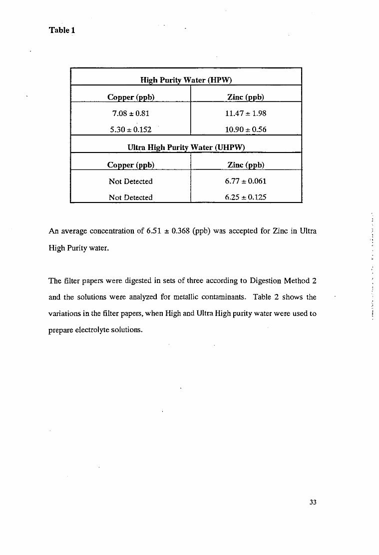
solutions were analyzed. Table 1 shows the differences in metallic concentrations
between the two grades of water.
32
Tablet
Hh!h Purity Water (HPW)
Copper (ppb) Zinc (oob)
7.08 ± 0.81 11.47 ± 1.98
5.30 ± 0.152 10.90 ± 0.56
Ultra High Purity Water (UHPW)
Copper (ppb) Zinc (ppb)
Not Detected 6.77 ± 0.061
Not Detected 6.25 ±0.125
An average concentration of 651 ± 0.368 (ppb) was accepted for Zinc in Ultra
High Purity water.
The filter papers were digested in sets of three according to Digestion Method 2
and the solutions were analyzed for metallic contaminants. Table 2 shows the
variations in the filter papers, when High and Ultra High purity water were used to
prepare electrolyte solutions.
33

Table 2
Hmh Purity Water (HPW)
Copper (ppb) Zinc (ppb)
6.70 ±0.603 30.74 ± 1.06
6.93 ± 0.79 33.61 ± 1.52
8.613 ± 0.362 28.32 ± 0.77
Ultra Hil!:h Purity Water (UHPW)
Copper (ppb) Zinc (ppb)
Not Detected 13.16 ± 1.06
Not Detected 18.27 ± 0.311
Not Detected 18.18 ± 0.339
3.00 ± 0.55 3240 ± 4.391
The results in Table 2 show that Zn was the major contaminant in the filter papers.
Although there is a reduction in the amounts of Copper and Zinc, when Ultra High
Purity Water was used, the possiblilty of an extraneous result appearing can not be
ruled out, since variations between individual filter papers do occur. However, the
values for Cu and Zn do not exceed 3 ppb and 33.61 ppb respectively for these
metals.
34

3.1 RECOVERY STUDIES
In order to evaluate the accuracy of an analytical method, a suitable reference
material of known metal concentration has to be subjected to the conditions set
out by the analytical method. Adeloju [32] used reference materials such as
animal muscle, bovine liver, oyster tissue and orchard leaves to compare the
recovery of metals from several wet digestion and dry ashing methods suited
speciffically for voltammetric trace metal analysis [32]. Ideally the matrix
composition of the matrix of the sample and the reference material should be the
same, so that any errors that may arise during the different stages of the analytical
method may be realised and assessed.
However, for this study no suitable reference material could be obtained. Instead
a recovery study of the metals from filter papers spiked with known amounts of
metals was evaluated. The percentage recovery of the metals give an indication of
the amount of metal released during the digestion procedure, which in turn
indicates whether or not the matrix which traps the metal has been completely
destroyed. The types of errors which may possibly arise from spiking a particular
matrix with the analyte metals are; inaccuracies in the actual spiking procedure
itself or adsorption onto the surfaces of the glass containers. Such errors lead to
lower recovery percentages. Conversely, higher recovery percentages are an
indication that contamination of the sample may have occured. Contamination of
this nature generally occurs as a consequence of impure reagents or carryover.
An airborne metal pollutant collected onto a filter paper medium must be viewed
as being surrounded by two matrices. The first being the organic or inorganic
moiety to which the metal is attached; as in the case Alkyl Lead compounds. The
second matrix is the filter paper itself onto which the metal pollutant is trapped.
These matrices must be removed so that the metal alone is available for analysis.
35

Interferences which occur from contributions by the matrix show up as
asymmetrical or distorted peaks in Voltammetric analysis.
Recovery studies using Digestion Methods 1 were performed and the recovery
percentages of the metals from the reagents and filter papers. With this digestion
method it was observed that a small volume of Sulphuric acid still remained in the
volumetric flask after digestion. The remaining acid was made up to 10.0 ml with
water. A 3.0 ml aliquot of this solution was then diluted to 10.0 ml with
electrolyte solution and then analyzed.
Tables 3 and 4 show the recovery percentages which were obtained. The metals
were determined simultaneously by scanning the sample solutions from -800 mV
to 100 mV. Zinc was not used in these recovery studies, since its half wave
potential (-1000 mV) occurs outside this voltage range; only the half wave
potentiaIs of Cadmium, Lead and Copper occur in this range and can thus be
determined simultaneously. Furthermore, the pH of the solution was 1.1 which is
not suitable for the determination of Zinc; a pH between 2.1 and 4.0 is required,
since the reduction wave of Hydrogen overlaps with the stripping peak of Zinc at
low pH values.
36

Table 3
Recoveries from Reagents
Number Metal Spike Recovery Recovery
(ppb) (ppb) (% )
Blank! Cd 0.9 1.49 165.56
Pb 0.9 0.76 84.44
Cu 4.5 3.59 79.78
Blank3 Cd 2.7 2.45 90.74
Pb 2.7 2.53 93.70
Cu 135 11.16 82.67
Blank 4 Cd 3.6 3.16 87.78
Pb 3.6 2.6 72.22
Cu 18.0 18.1 100.56
BlankS Cd 4.5 4.44 98.67
Pb 4.5 4.5 100.0
Cu 22.5 31.76 141.16
37

Table 4
Recoveries from Filter Papers
Number Metal Spike Recovery Recovery
(ppb) (ppb) ( %.)
Sample 1 Cd 0.9 1.54 171.11
Ph 0.9 0.81 90.00
Cu 4.5 6.93 154.00
Sample 3 Cd 2.7 2.53 93.70
Ph 2.7 2.61 96.67
Cu 13.5 15.52 114.96
Sample 4 Cd 3.6 3.28 91.11
Ph 3.6 3.11 86.39
Cu 18.0 17.52 97.33
SampleS Cd 4.5 4.12 91.56
Ph 4.5 4.54 100.89
Cu 22.5 25.91 115.16
38

Both sets of results show that extremely high recovery percentages were obtained
at the low spiked concentrations for Cadmium and Copper. This can be attributed
to contamination in the system, as a consequence of impure reagents or sample
carryover. In the case of the Cadmium results the contamination is due to carry
over, since no Cadmium was detected in neither the reagents nor the filter papers.
The contamination of Copper is largely due to the presence of this metal in the
background electrolyte, since High Purity Water and not Ultra High Purity Water
was used to prepare the electrolyte solution. However, the results in the above
tables should be appreciated when working with extremely dilute solutions since
the possibility of contamination errors occurring is large.
The results obtained in Tables 3 and 4 were calculated using the Standard
Addition Formula. These results were compared to those obtained from
Calibration Curves. The purpose of this comparison was to establish whether or
not an agreement existed between the two quantitative methods. The calibration
curves were set up by digesting a filter paper and making it up to 10 ml with
water. A 3 ml aliquot of this solution was then diluted to 10.0 ml with electrolyte
solution and transfered into the polarographic cell for analysis. The currents were
recorded as 10 f.ll amounts of standard metal solutions were added to the bulk
solution. Calibration curves such as those shown in the Appendix (Figures 1, 2
and 3) were generated for Copper, Lead and Cadmium. Table 5 shows the results
obtained from the Calibration Curves and Standard Addition Formula.
39

TableS
Standard Addition Formula vs Calibration Curve
Number Metal Formula Graph Percentage
(ppb) (ppb) Deviation
Blankl Cd 1.49 1.21 18.79
Pb 0.76 0.66 13.15
Cu 3.59 4.55 26.74
Blank 3 Cd 2.45 2.12 13.47
Pb 2.53 2.09 17.39
Cu 11.16 10.31 7.62
Blank 4 Cd 3.12 3.02 3.21
Pb 2.60 2.87 10.39
Cu 18.10 17.63 2.60
BlankS Cd 4.44 4.12 7.21
Pb 4.50 3.95 12.22
Cu 31.76 20.29 36.11
Sample 1 Cd 1.54 1.21 21.42
Pb 0.81 0.65 19.75
Cu 6.95 7.71 10.94
Sample 3 Cd 2.53 2.60 2.76
Pb 2.61 2.22 14.94
Cu 15.52 15.02 3.33
Sample 4 Cd 3.28 3.02 7.93
Pb 3.11 2.69 13.51
Cu 17.52 16.6 5.25
SampleS Cd 4.12 4.12 0.00
Pb 4.54 3.75 17.40
Cu 25.91 20.29 21.69
40

At these Iow concentrations of metals there is good agreement between the two
methods and the results show that measurement by either of the two quantitative
methods are equally valid Similar results were obtained by Komy [3] whilst
determining metals in rain water, in the concentration range 0.15 to 50 ug/l. Since
it was observed that the amount of residual Sulphuric acid remaining after
digestion varied from sample to sample it is to be expected that the characteristics
of the sample solution will also change. Thus variations in the results between the
methods of quantitation are to be expected. However, from the agreement in the
between the two quantitative methods it can be concluded that the destruction of
the filter paper matrix was complete.
41
3.2 DIGESTION METHOD 1: APPLIED TO AIR SAMPLES
The airborne particulate matter which was collected onto filter papers were
digested according to Digestion Method 1. The resulting solution after digestion
was a dark grey coloured solution containing fine particles. TIris observation
implied that the digestion was incomplete. When further additions of 2.0 ml of
Nitric acid were made the dark grey solution eventually became colourless. The
amount of Nitric acid added to the digestion solution varied from one sample to
another and up to 8.0 ml of Nitric acid had to be added in some instances. TIris
digestion method became time consuming and showed that the initial 5.0 ml Nitric
acid added was insufficient for the complete destruction of the matrices. Another
problem encountered with this method was that spot heating caused some of the
volumetric flasks to crack, thus making this method unsuitable for analysis. 1bis
digestion method was not pusued further for the digestion of airborne particulate
samples.
3.3 RECOVERY STUDIES: DIGESTION METHOD 2
Since it was observed that Digestion Method 1 was not suitable for the complete
destruction of the airborne particulate matter matrices, recovery studies evaluating
Digestion Method 2 had to be performed. In this digestion method a higher
temperature and larger volumes of acids were used. Tables 6 and 7 show the
recovery percentages of the metals from reagents and filter papers spiked with
known concentrations of the metals. The metals were determined using the
instrumental conditions set out in the experimental chapter.
42

Table 6
Recoveries from Reagents
Number Metal Spike Recovery (% )
(ppb) (ppb) Recovered
Sample 1 Cd 8.82 9.48 107.48
Pb 2.45 2.51 102.45
Cu 18.93 20.22 106.81
Zn 32.90 35.28 107.20
Sample 2 Cd 8.82 9.58 108.62
Pb 2.45 2.51 102.45
Cu 18.93 19.54 103.22
Zn 32.90 33.50 101.82
Sample 3 Cd 8.94 8.55 95.64
Pb 2.51 2.24 89.24
Cu 19.54 20.36 104.19
Zn 33.50 32.45 96.87
Sample 4 Cd 8.94 9.31 104.14
Pb 2.16 2.19 101.39
Cu 19.10 19.80 103.66
Zn 32.95 33.80 102.58
SampleS Cd 8.73 8.90 101.94
Pb 2.21 2.34 105.88
Cu 18.5 19.18 103.68
Zn 33.49 39.69 118.51
Sample 6 Cd 8.73 8.12 93.01
Pb 2.21 2.25 101.81
Cu 18.73 18.74 100.05
Zn 33.49 38.45 114.8143

Table 7
Recoveries from Filter Papers
Number Metal Spike Recovery Percentage
(oob) (oob) Recovered
Sample 1 Cd 8.86 8.68 98.41
Pb 2.17 2.25 103.69
Cu 18.38 19.41 105.60
Zn 33.10 36.46 110.15
Sample 2 Cd 8.86 8.60 97.07
Pb 2.17 2.25 103.69
Cu 18.38 20.04 109.03
Zn 33.10 33.58 101.48
Sample 3 Cd 8.87 8.24 92.90
Pb 2.27 2.27 100.00
Cu 19.65 26.47 134.71
Zn 32.91 32.86 99.85
Sample 4 Cd 8.87 8.24 92.90
Pb 2.24 2.21 98.66
Cu 19.65 19.35 98.68
Zn 32.91 33.86 98.85
SampleS Cd 9.05 9.74 107.62
Pb 2.22 2.35 105.86
Cu 19.08 19.95 104.56
Zn 32.78 37.70 115.01
Sample 6 Cd 9.05 9.95 109.94
Pb 2.22 2.29 103.15
Cu 19.08 19.57 102.57
Zn 32.78 46.09 140.60

The values of 134.71% and 140.60% for Cu and Zn in Table 7 were rejected and
the statistical analysis performed on the remaining data is given in Table 8.
TableS
Recoveries from Reagents
Metal Average (%) Std. Dev %RSD
Cd 101.76 6.316 6.21
Pb 100.54 5.759 5.73
Cu 103.60 2.164 2.09
Zn 107.23 7.901 7.37
Recoveries From Filter Papers
Metal Average (%) Std. Dev %RSD
Cd 99.81 7.330 7.34
Pb 102.51 2.670 2.60
Cu 104.09 3.824 3.67
Zn 105.07 7.132 6.79
The results in Table 8 show that high recovery percentages with relative standard
deviations below 10% are possible.
Adeloju [32], studied the recovery ofmetals, from different matrices, using several
digestion methods and found Digestion Method 2 gave recovery percentages
between 95% to 100%. The results obtained here confirm his findings.
+5

3.4 DIGESTION METHOD 2: APPLIED TO AIR SAMPLES
The digested sample solutions obtained by this method were colourless and
showed no undigested matter, this could be attributed to the higher digestion
temperature and the repeated additions of Nitric acid (5.0 ml aliquots). A typical
voltammogram (scanned between -900 to 150 mY) for the electrolyte solution
prior to sample analysis is shown in Figure 4 and the metals found in the sample
solution are shown by Figures 5 - 7. The symmetrical peaks are an indication that
the digestion of the matrices was complete. All airborne particulate samples were
thus digested using this method. A scan of the background electrolyte was
performed each time prior to the analysis of a new sample, in order to minimize
contamination from sample carryover.
46

VOLTAMMOGRAM of ELECTROLYTE
10 rnl of Electrolyte solution
IAMEL 4331,----------------~
I
I,
cr::::r.,
2
5 '---,-'----r-,-,--r--.---i--,--r---r---,-..,.----.-,----'
e .1 -e .1 -8.3 -e.5 -6.7 -8.9
POTENTIAL, U
Figure 4
47

VOLTAMMOGRAM of COPPER
(1) 10.034 ml Sample solution(2) 10.034 ml Sample solution + 18.64 ppb Cu(3) 10.034 ml Sample solution + 37.27 ppb Cu
IlUtE!. 433]
8
,
3
6L--'--,---.----r------r-..,.---,_--.-----,--_~...--J
8.1 -£J.1 -8.3 -a.S -8.7 -8.9
POT.ENTIAL, U
Figure 5
48

VOLTAMMOGRAM of LEAD
(1) 10.034 ml Sample solution(2) 10.034 ml Sample solution + 10.29 ppb Pb(3) 10.034 ml Sample solution + 20.58 ppb Pb
IAl1EL 4331
6
""' /1"cr::::L. I
, 18- 1\\)!- 11Z
w 28-
\¥Ia::a::::::J
3e - \luV3
46 I .. I . •e.1 -£I .1 -£I .3 -a.5 -5.7 -8.9
POTENTIAL, l)
Figure 6
49

VOLTAMMOGRAM of ZINC
(1) 10.046 ml Sample solution(2) 10.046 ml Sample solution + 60.12 ppb Zn(3) 10.046 ml Sample solution + 120.23 ppb Zn
IAMEL 4331 ,.---------------------,
, 18r-Z
W
G::
G:: 38
:::::>U
3
u-1
POT E· N T I A L ;
58 '-------.------.-----.......-----'-a.S
Figure 7
50

The Standard Addition Graphs in the Appendix (Figures 8, 9 and 10) were used to
to calculate the concentrations of the metals from the voltammograms above.
These results were compared to those calculated by using the Standard Addition
Formula. Table 9 show the agreement in the results between the graphical method
and the formula.
Table 9
Formula n Graphical Method
Metal Formula Graphical Method
Cu 14.15 ppb 14.50ppb
Pb 10.26 ppb 10.29ppb
Zn 49.93 ppb 52.55 ppb
The concentration of the metal per cubic meter of air was calculated using the
formula below:
Metal(ug/m3) =C(unk) x Factor ... 28.8 m3
where, Factor = total sample volume (ml) ... volume of sample aliquot (ml)
The total sample volume of air collected over a 24 hour period was 28.8 m3.
51

3.5 CONCENTRATION VARIATIONS OF METALLIC
POLLUTANTS
The Differential Pulse Anodic Stripping Voltammetric technique procedure
developed in the experimental section was used for the determination of airborne
metals in the atmosphere.
Analyses were performed on 77 samples, which were collected randomly from
February to December 1992. The samples were collected over a 24 hour period
and thus reflect the daily averages of the metals detected. Air samples were not
collected during January and June since the campus was closed for the summer
and winter holidays. All samples were collected from one monitoring site which
was located close to the main enterance gate of the campus. Since a high volume
of motor vehicles passes through the gates daily, it is expected the metal pollutants
are derived mainly from their emissions.
Copper, Lead and Zinc were the only metals that were detected; no Cadmium was
detected in any of these samples. Table 10 shows the results obtained for these
metals during the year 1992 and Figures 11 - 13 show graphical representations of
the metals found in the samples.
52

Table 10
Date Number Cu Pb Zn
(llg/m3) (llg/m3) (llg/m3)
February 17-18 1 ND 2.13 24.69
25-26 2 3.52 0.69 14.30
26-27 3 4.88 2.35 35.16
28-29 4 25.95 6.46 42.37
March 16-17 5 3.81 1.30 19.94
23-24 6 6.46 2.03 19.59
April 13-14 7 ND 1.38 17.74
22-23 8 ND 2.61 41.94
23-24 9 ND 0.61 14.09
28-29 10 3.48 2.39 NDMay 4-5 11 2.17 0.71 8.10
5-6 12 6.3 1.92 31.55
11-12 13 14.88 12.43 176.64
12-13 14 14.88 7.55 123.26
13-14 15 2.90 2.07 40.66
14-15 16 2.31 0.87 15.71
26-27 17 2.45 1.78 5.72
July 10-11 18 1.08 0.62 12.11
13-14 19 1.21 1.00 10.74
14-15 20 14.83 1.77 28.67
17-18 21 1.24 0.30 9.19
20-21 22 1.94 0.40 5.41
22-23 23 2.26 0.44 8.98
23-24 24 1.61 1.33 9.19
27-28 25 1.11 0.91 ND28-29 26 LlO 0.77 7.87
29-30 27 1.76 Ll6 12.38
53
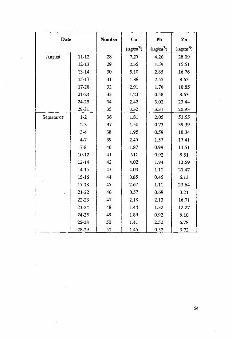
Date Number eu Ph Zn
(Jlg/m3) (Jlg/m3) (Jlg/m3)
August 11-12 28 7.27 4.26 28.09
12-13 29 2.35 1.59 15.51
13-14 30 5.10 2.85 16.76
15-17 31 1.88 2.55 8.63
17-20 32 2.91 1.76 10.85
21-24 33 1.23 0.58 8.63
24-25 34 2.42 3.02 23.44
29-31 35 3.32 3.31 20.93
September 1-2 36 1.81 . 2.05 53.55
2-3 37 1.50 0.73 39.39.3-4 38 1.95 0.59 10.34
4-7 39 2.45 1.57 17.41
7-8 40 1.87 0.98 14.51
10-12 41 ND 0.92 8.51
12-14 42 4.02 1.94 13.59
14-15 43 4.04 1.11 21.47
15-16 44 0.85 0.45 6.13
17-18 45 2.67 1.11 23.64
21-22 46 0.57 0.69 3.21
22-23 47 2.18 2.13 16.71
23-24 48 1.44 1.32 12.27
24-25 49 1.89 0.92 6.10
25-28 50 1.41 2.52 6.78
28-29 51 1.45 0.52 3.72
54

Date Number Cu Pb Zn
(1lg/m3) (p.g/m3) (llg/m3)
October 30-(Sept) 52 1.23 0.82 7.95
-1
1-5 53 1.34 1.08 7.19
5-6 54 1.85 1.06 31.05
7-8 55 1.57 0.48 6.46
8-10 56 1.05 1.05 8.65
10-12 57 0.81 0.55 3.71
12-13 58 1.09 0.89 30.15
13-14 59 1.67 0.89 14.08
14-15 60 0.77 0.21 0.44
15-19 61 0.82 ND 2.95
19-20 62 1.45 0.43 5.94
20-21 63 1.06 0.43 5.97
21-22 64 1.32 0.49 11.05
22-23 65 0.97 0.43 6.95
26-27 66 1.30 0.9 10.71
November 17-18 67 1.20 0.8 10.62
19-20 68 1.07 0.46 5.34
20-23 69 0.96 3.19 4.44
23-24 70 1.30 0.55 6.45
24-25 71 1.13 0.34 11.60
25-26 72 1.13 0.83 6.74
26-27 73 2.06 0.89 8.54
December 1-2 74 0.8 0.17 ND
2-3 75 1.12 0.59 3.95
7-8 76 ND 0.33 5.56
8-9 77" 0.49 0.33 23.35
55

CONCENTRATION PROFILE of COPPER
••3 '\ .
~ ~.--. .o L L L __L __-l 1 J I I' f 71~-,-·~i~ I - I
1 6 11 16 21 26 31 36 41 46 51 56 61 66 71 76
Sample NumberFIGURE 11
g.:
Copper (ug/m3)30
27 1 •I
24 ,-
21 ,-
18 ,-
151- 11 • •
12
9 1- I \ I \ 1\ •6

CONCENTRATION PROFILE of LEADLead (ug/m3 )
15 ,,-----------------------------,
12 ,-
91-
6' -+
-+
6
31-1 \ -+-+1\ A It
-++-+ -++ Io I I
1
~ FIGURE 12
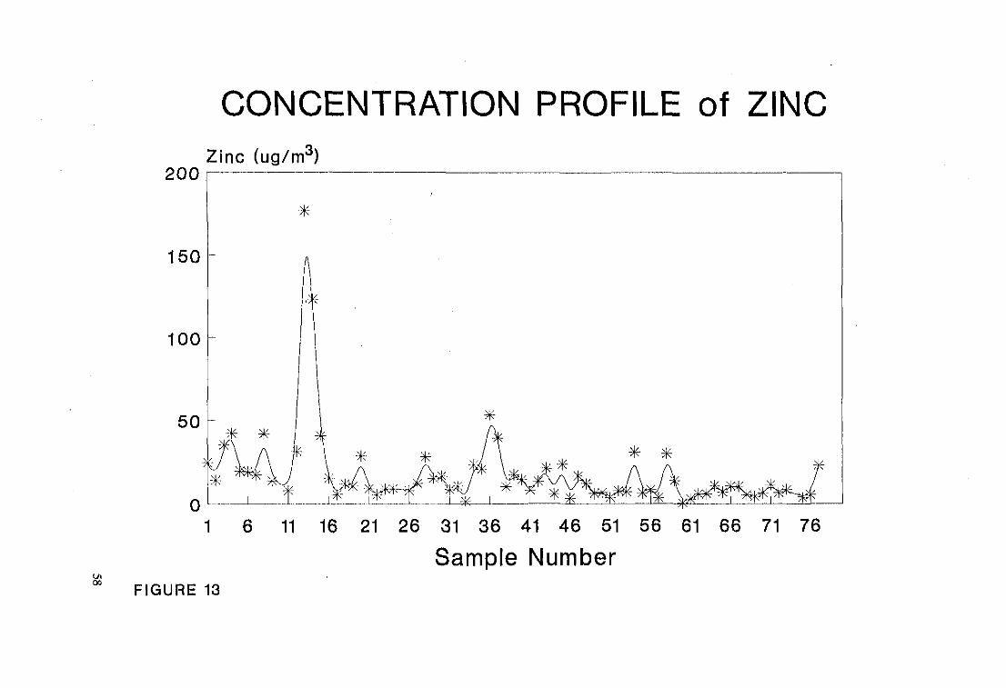
CONCENTRATION PROFILE of ZINC
200 ~~C (u~/m3)------
*150 .-
100
*501-
-l'~ ~JK \* * ;- '- , * *~ ~.~ 7\r .~ * -o l~_~ '-_~t :L~~**£'~1 *' -: ~ _:-:, -~~~~~
1 6 11 16 21 26 31 36 41 46 51 56 61 66 71 76
Sample NumberFIGURE 13
u,ao

The positions at which peaks occur relative to the sample number are tabulated in
Table 11. The positive and negative signs indicate the presence and absence of
peaks.
Table 11
Sample Number Copper Lead Zinc
1-6 + + +
11-16 + + +
18-21 + + +
26-31 + + +
33-36 + + +
41-46 + + +
46-51 - + +
51-56 - + +
56-61 - + +
These plots show that the peaks and troughs of the metals coincide closely with
each other, thereby indicating that the metals are emitted from a common source,
namely the emissions from motor vehicle exhaust systems. Analysis of exhaust gas
by Atomic Absorption Spectroscopy showed that eu and Zn are also emitted from
motor vehicle exhaust systems [37].
59
The average concentrations and standard deviations for the metals as determined
for the year 1992 are therefore; Cu (3.77 :!: 3.23), Pb (1.69 :!: 1.11) and Zn
(20.31:!: 14.7) micrograrns per cubic meter. Since the standard deviation indicates
the distribution about the mean it can be deduced that there is more than one
factor contributing towards the concentration of metals found in the atmosphere.
These factors can include the volume of traffic flow and or the climatic conditions.
60

3.6 MONTHLY METAL AVERAGES
The monthly average concentrations of the metals are given in Table 12 and
represented graphically by the bar graph in Figure 14.
Table 12
Month eu Pb Zn Total
(!1g!m3) (!1g!m3) (!1g!m3) (!1g!m3)
1
2 11S 2.9 29.1 43.5
3 5.1 1.7 19.8 23.6
4 3.48 1.7 24.6 29.8
5 6.3 3.9 57.4 67.6
6
7 2.8 0.9 11.6 15.3
8 3.3 2S 15.7 21.5
9 2.0 1.2 16.1 19.3
10 1.2 0.7 10.2 12.1
11 1.26 1.01 7.68 10.0
12 0.80 0.36 10.95 12.1
Average 3.77 . 1.69 20.31 25.6
Std. Dev. 3.23 1.11 14.7 17.87
61

Monthly AveragesCOPPER, LEAD and ZINC
Concentration (ug/m3 )6 0 ,-------~-----~~-----------~
50 ,.
40 ~
30 ,-
20 ,-
1: :,~~IY~I± LulilJ , IlJi.1JLJ ..JJ~
'"'"
Jan Feb Mar Apr May Jun Jul Aug Sep Oct Nov Dec
Month
_ Copper _ Lead Zinc
FIGURE 14

Higher concentrations of metal were found during the first half of the year than
during the second half. February showed an a extremely high eu result; this high
value was as a consequence of a veld fire which occured close to the campus on
the 28-29th of February. Cu is released during the combustion of plant material.
The total concentration of the metals for each month is shown in Figure 15. Since
it is not possible to obtained a true average background concentration for the
metals, the yearly average was used for this purpose (Average 25.6 flg!m3), thus
the increase or decrease in the metal concentrations during the year were
compared relative to this average.
63

Total Metal ConcentrationsConcentration (ug/m3 )
7 0 I------~--~---·--------·----------·-·-·----- 1
60
50 ,-
40 ,-
30'~ F:::'-:::;='J---~~"---I--·-i~-···'·_+--~--,-,,--_·_~~-- . ----~~----.............--~~~-~
~LL~_L_L, L_,---I] ,,,',~~_~_L_~_"o '-- __'- '--'--1
20-
10'
Jan Feb Mar Apr May Jun Jul Aug Sep Dct Nov Dec
Month
[---] Metals -.- Average
~
FIGURE 15

The variations in metal concentr<itions with different periods show that there are
factors which attribute towards this phenomenon. It is well known that the
atmosphere uses. meteorological mechanisms which aid in the removal of
pollutants. These mechanisms include stirring or turbulant diffusion,
photochemical transformations, by rainout or fallout [36].
3.7 METEOROLOGICAL DATA FOR 1992
The concentration of the metal pollutants was plotted against the meteorological
data, (temperature, wind speed, relative humidity and rainfall) in order to establish
whether or not any trends exist between the data. Figures 16 to 19 show the
plots obtained and the meteorological data are shown in Tables 13 to 15.
65

CONCENTRATION vs TEMPERATURE
10
20
15
25
,--,---15
,__El
--B~
20 ,. 0
10
o
40 ,-
Concentration (ug/m3 ) Temperature (QC)70 ,------- 130
60f---~~
30 ,-
50 ,-
Jan Feb Mar Apr May Jun Jul
MonthAug Sep Oct Nov Dec
---8- Maxi Temp. (QC) -*- Mini Temp. (QC) Metals
~FIGURE 16

CONCENTRATION vs RELATIVE HUMIDITY
40
60
80
I----r----r--i 20
I. L __J L.....J.... I I .1 L __..1--.I----1 I I I I I I I I I --.J 0
Concentration (ug/m3) Relative Humidity (0/0)70 1------------ = ~ 100
60
50
40
30
20
10
oJan Feb Mar Apr May Jun Jul Aug Sep Oct Nov Dec
Month
--u- at 8:00 -"*- at 14:00 ----(j- at 20:00
---[>--- Average (%) [~:J Metals
~FIGURE 17

CONCENTRATION vs RAINFALL
Rainfall (mm)-- 160
140
120
-. 100
80
60
40
20
o 0
10 .-
50 .-
Concentration (ug/m3)70,---
r=
20 .-
40 .-
30
60
Jan Feb Mar Apr May Jun Jul Aug Sep Oct Nov Dec
Month
--0-- Rainfall (mm) Metals
&lFIGURE 18

CONCENTRATION vs WIND SPEEDConcentration (ug/m3 )
70,Wind Speed (m/s)
------" 10
2
6
4
~ -18,.---
'~
--,~-=~"x
10'-
0' ~., I'-[! 1·1"1 ""I'....J I I~I )-1":1 I"-'I-';! 1:;:'1,·"1 1'<,'1':;;'-' "':1';110
Jan Feb Mar Apr May Jun Jul Aug Sep Oct Nov Dec
Month
50 .-
40 ,
30 ,
20 .-
60
-EJ-- at 8:00 --x- at 14:00 --0- at 20:00 -8- Average Cl Metals
$FIGURE 19

Table 13
Relative Humidity ( %.)
Month 8:00 14:00 20:00 Avel"32e
January 72 54 72 66
February 79 56 74 69
March 84 58 78 73
April 89 57 81 76
May 89 65 83 79
June 87 61 83 77
July 86 61 81 76
August 86 54 79 73
September 89 60 79 76
October 82 60 80 74
November 72 53 78 67
December 66 51 73 63
70

Table 14
Wind SDeed ( m1s )
Month 8:00 14:00 20:00 Ave~e
January 6.1 8.5 8.5 7.7
February 2.8 6.7 5.8 5.1
March 3.4 6.8 5.6 5.3
April 1.4 4.9 3.1 3.1
May 2.7 4.2 2.0 3.0
JUDe 33 6.0 3.6 4.3
July 3.2 5.6 3.6 4.1
August 1.7 4.7 2.7 3.0
September 2.1 5.7 3.8 3.9
October 5.2 8.4 6.2 6.6
November. 4.1 7.6 5.5 5.7
December 4.6 8.2 6.7 6.5
71

Table 15
Temperature eC)
Month Minimum Maximum Rainfall (mm)
January 16.8 25.5 1.4
February 16.2 26.2 29.5
March 15.4 25.5 13.0
April 11.1 21.9 85.8
May 93 18.9 51.2
June 7.5 17.6 145.1
July 7.8 16.6 91.7
August 6.7 17.8 43.3
September 9.1 17.8 62.3
October 11.2 20.6 77.1
November 12.4 23.5 10.7
December 14.6 24.3 5.2
72

3.8 METEOROLOGICAL FACfORS INFLUENCING AIR POLLUTION
The amount of pollutants entering the atmosphere is the largest factor influencing
air pollution. It has been observed that although emissions into the atmosphere
remain steady for long periods, large variations do occur from one day to the
other. These variations are a consequence of changes in certain atmospheric
conditions [35].
Figure 15, shows that the concentration of the metals are above the yearly average
value (25.3 j.l.glm3) during the first half of the year as compared to the below
yearly average in the second half. An increase in concentration occurs from March
to May, while a decrease occurs from August to November. The high
concentration of eu resulted in a larger total metal concentration for February.
Wind strength and Air stability are important atmospheric factors which affect the
dispersion of pollutants, since they determine how rapid pollutants are diluted with
the surrounding air once they have been emitted. A direct consequence of wind
speed is that; higher wind speeds remove pollutants more rapidly away from the
source, it also causes the air to be more turbulent thus diluting the pollutants with
the surrounding air. This effect is clearly demonstrated in Figure 19, where the
concentration increased from March to May with a corresponding decrease in the
wind speed. The converse is true for increasing wind speeds where the
concentration decreased from August to November (Figure 19).
73
When the air is unstable, the air currents carry smoke and exhaust fumes upwards
were it is mixed with the cleaner air and dispersed by the winds above. The
decrease in concentration with increasing temperature, from August to November
(Figure 16) corresponds to the formation of an unstable air currents which result
from a warmer surface temperature. The lower concentration of pollutants is
reinforced by the increase in wind speed from August to November (Figure 19).
The lower pollutant concentration for July as compared with that of August is due
to the higher wind speed for July. A stable air condition results in Temperature
Inversion, (cooler air layer is trapped by a warmer air layer above it) resulting in
the suppression of vertical mixing and dilution of pollutants. In such instances the
pollutant concentration remains high [35].
Rain, hail or combinations thereof are forms of precipitation. Precipitation result in
pollutants being removed from the atmosphere before dispersion has taken place.
The concentration of pollutants is at a maximum concentration during the initial
stages of rainfall [31]. It is therefore expected that the concentration of the
pollutants should be lower during months of higher rainfall. This effect is observed
in July, August, September and October (Figure 18).
The temperature of the atmosphere depends on the rate at which energy from the
sun reaches the earth. Temperature is not a constant and since it varies with
factors such as height, latitude, season, time of day, etc. During the day the solar
radiation is absorbed by the ground resulting in a warming of the earth's surface.
At night the radiation of energy by the earth's surface will result in its cooling and
result in an inversion layer. As a consequence pollutants accumulate during the
night a few hundred meters above the ground. These pollutants are then carried to
the ground in the morning as the earth's surface begins to warm; hence the
pollution level will thus be increased at morning time and then decrease as the day
becomes warmer [38]. Figure 16 indicates that the increase in concentration with
74

decreasing temperature is a result of temperature inversion which had occurred
during the day.
The relative humidity depends on the amount of water vapor required to saturate
the air and is influenced by temperature. Generally a decrease in temperature
increases the relative humidity, while an increase in temperature will result in a
decrease in the relative humidity [35]. When the humidity is low the
concentrations of suspended particulate pollutants increases; this accounts for the
increase in pollutant concentration observed from March to May in Figure 17.
High humidity, result in fog conditions, and can block solar heating of the ground
surface and result in an unstable air flow (the life of inversion layers is increased)
as consequence the concentration of the pollutants increases or remains high.
Figure 17 also shows that the pollutant concentration decreased from September
to November as the relative humidity decreased. Since the relative humidity is
low, the wind speed and temperature high for December is observed, a pollutant
concentration lower than November is expected, however this is not the case, thus
implying that a stable air condition has occurred as a result of temperature
inversion. It is apparent that temperature inversions occur mainly from December
to May whereas stable air conditions occur from July to November.
75

CHAPTER 4
CONCLUSIONS
An analytical procedure was developed, using Differential Pulse Anodic Stripping
Voltammetry technique as an analytical tool, for determining trace amounts of
metal pollutants in the atmosphere. This has been successfully applied for the first
time in the Republic of South Africa for airborne Copper, Lead and Zinc. These
metals were emitted from motor vehicle emissions traversing past the sampling
site.
The absence of a sediment after digestion and spurious peaks on the
voltammograms implied that digestion was complete. Although the method of
Standard Addition was used for quantitation, the use of a Calibration curve for
quantitation is possible, and must be optimized, since good agreement between the
two methods of quantitation was observed.
The variations in metal pollutants with the meteorological data has emphasized the
influence of climatic factors such as wind speed, temperature and relative humidity
in the cleansing of the atmosphere. Since the influence of climatic factors has been
treated on a qualitative basis, no quantitative mathematical model could be
generated. However, a quantitative evaluation is possible if the frequency of
monitoring is increased over a longer period and at more than one monitoring site.
The analysis time and sampling equipment for such a quantitative evaluation can
become extremely costly and was not actively pursued in this instance.
76

APPENDIX jjjjjjjjjjjjjjjjjjjjjjjjjjjjjjjjjjjjjjjjj
n jjjjjjjj

COPPERCALIBRATION CURVE
Current (uA)
•
•
•
30 3510 15 20 25
Concentration (ppb)5
//
./
11/vo.>--.----'--------'----------'------'-----'--------'-----
o
FIGURE 1
78

CADMIUMCALIBRATION CURVE
Current (uA)
I10 ~
(
I
7/
/
!
I5 f- /
1/I /i/
0/o 1 2 345
Concentration (ppb)6 7
FIGURE 2
79

LEADCALIBRATION CURVE
Current (uA)1.6
1
,-----------------/-/-y-'----,
1.4 ri
1.2
1
0.8 L
o 1 2 3 4 5
Concentration (ppb)6 7
FIGURE 3
80

COPPERSTANDARD ADDITION METHOD
Current (uA)4,-------------------:1
I
3~I
2
V1 ,
I
4010 20 30
Concentration (ppb)
io i -----'- --'-- '---__~
o
FIGURE 8
81

LEADSTANDARD ADDITION METHOD
Current (uA)40c---------------~___,
30
20
T
10 ~
255 10 15 20
Concentration (ppb)
o '---'__---'---__----'-__----' -'--_------.1
o
FIGURE 9
82

ZINCSTANDARD ADDITION METHOD
Current (uA)50.-----------------,
40 r
I
30 1
•
20
40 60 80 100 120 140
Concentration (ppb)20
•
10 1I
oI---'-------'---------'-----~---"-------'----~
o
FIGURE 10
83
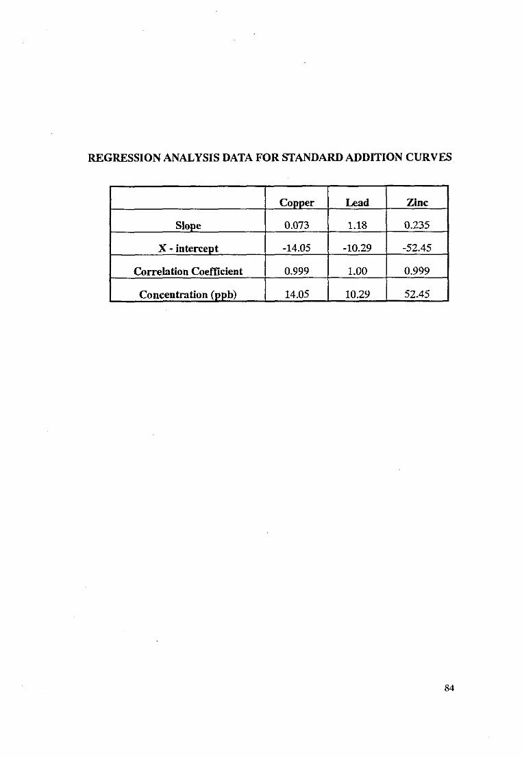
REGRESSION ANALYSIS DATA FOR STANDARD ADDITION CURVES
Copper Lead Zinc
Slope 0.073 1.18 0.235
X - intercept -14.05 -10.29 -52.45
Correlation Coefficient 0.999 1.00 0.999
Concentration (vpb) 14.05 10.29 52.45
84

REFERENCES
1 Stripping Analysis Principles, Instrumentation and Applications. Joseph
Wang, VHC Publishers Inc. (1985).
2. Ben-Bassat, A.H.I., Blindermann, J.M., Soloman, A., Anal. Chem. 47, 3,
534 (1975).
3. Komy, Z., Roekens, E., Van Grieken, R., Analytica Chemica Acta, 204,
179-187 (1988).
4. Vos, L., Komy, Z., Reggers, G., Roekens, E., Van Grieken, R., Analytica
Chemica Acta, 184, 271-280 (1986).
5. Numberg, H.W., Analytica ChemicaActa, 164, 1-21 (1984).
6. Valenta, P., Rutzel, H., Numberg, H.W., Stoepler, M., Z. Anal. Chern. 285,
25-34 (1977).
7. Nur Onar, A. and Temizer Aytekin., Analyst, 112,227 (1987).
8. Lippolis, M.T., Conialini, V., Galletti, G.c., Piccaglia, P., Analyst, 114,
1621 (1989).
9. Adeloju, S.B., Bond, A.M., Noble, M.L., Analytica Chemica Acta, 161,
303-314 (1984).
85

10. Adeloju, S.B., Bond, AM., Hughes, RC., Analytica Chemica Acta, 148, 55
(1983).
11. Adeloju, S.B., Bond, AM., Briggs, M.H., Anal. Chem. 57, 1386-1390
(1985).
12. Adeloju, S.B., Bond, AM., Briggs, M.H., Analytica Chemica Acta, 164,
181-194 (1984).
13. Yamashige, T., Yamamoto, M., Sunahara, H., Analyst, 114, 1071 (1989).
14. Pickford, CJ., Rossi, G., Analyst, 103,341-355 (1978).
15. Begnoche, RC., Risby, T.H., Anal. Chem. 47, 7,1041 (1975).
16. Harrison, P.R., Winchester, l.W., Atmospheric Enviroment, 5, 863-880
(1971).
17. Colovos, G., Wilson, G.S., Moyers, l., Analylica Chemica Acta, 64, 457
464 (1973).
18. Wandl, MA.E., Pougnett, MA-B.; Analyst, 111, 1249 (1986).
19. Beinrohr, E., Rojcek, l., Garaj, J., Analyst, 113, 1831 (1988).
20. Satake, M., Muira, l., Usami, S., Puri, B.K., Analyst, 114,813 (1989).
86
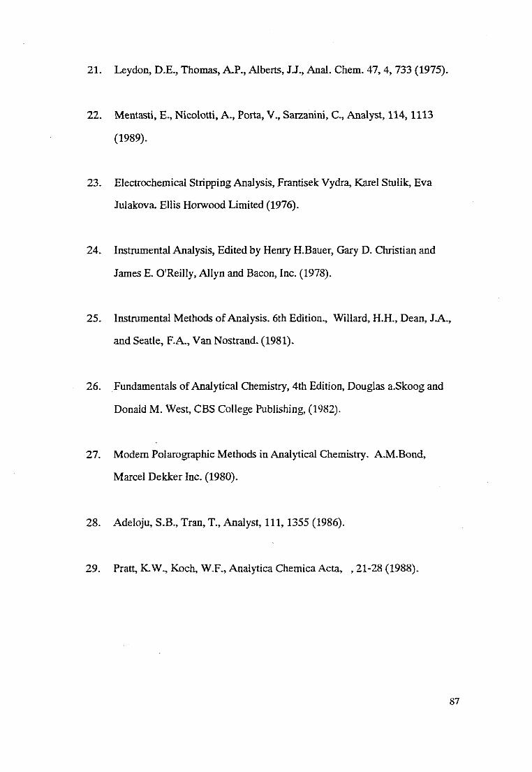
21. Leydon, D.E., Thomas, AP., Alberts, JJ., Anal. Chem. 47, 4, 733 (1975).
22. Mentasti, E., Nicolotti, A., Porta, V., Sarzanini, c., Analyst, 114, 1113
(1989).
23. Electrochemical Stripping Analysis, Frantisek Vydra, Karel Stulik:, Eva
Julakova. Ellis HOlWood Limited (1976).
24. Instrumental Analysis, Edited by Henry H.Bauer, Gary D. Christian and
James E. O'Reilly, Allyn and Bacon, Inc. (1978).
25. Instrumental Methods ofAnalysis. 6th Edition., Willard, H.H., Dean, JA.,
and Seatle, F.A., Van Nostrand. (1981).
26. Fundamentals ofAnalytical Chemistry, 4th Edition, Douglas a.Skoog and
Donald M. West, CBS College Publishing, (1982).
27. Modem Polarographic Methods in Analytical Chemistry. A.M.Bond,
Marcel Dekker Inc. (1980).
28. Adeloju, S.B., Tran, T., Analyst, 111, 1355 (1986).
29. Pratt, K.W., Koch, W.F., Analytica Chemica Acta, ,21-28 (1988).
87
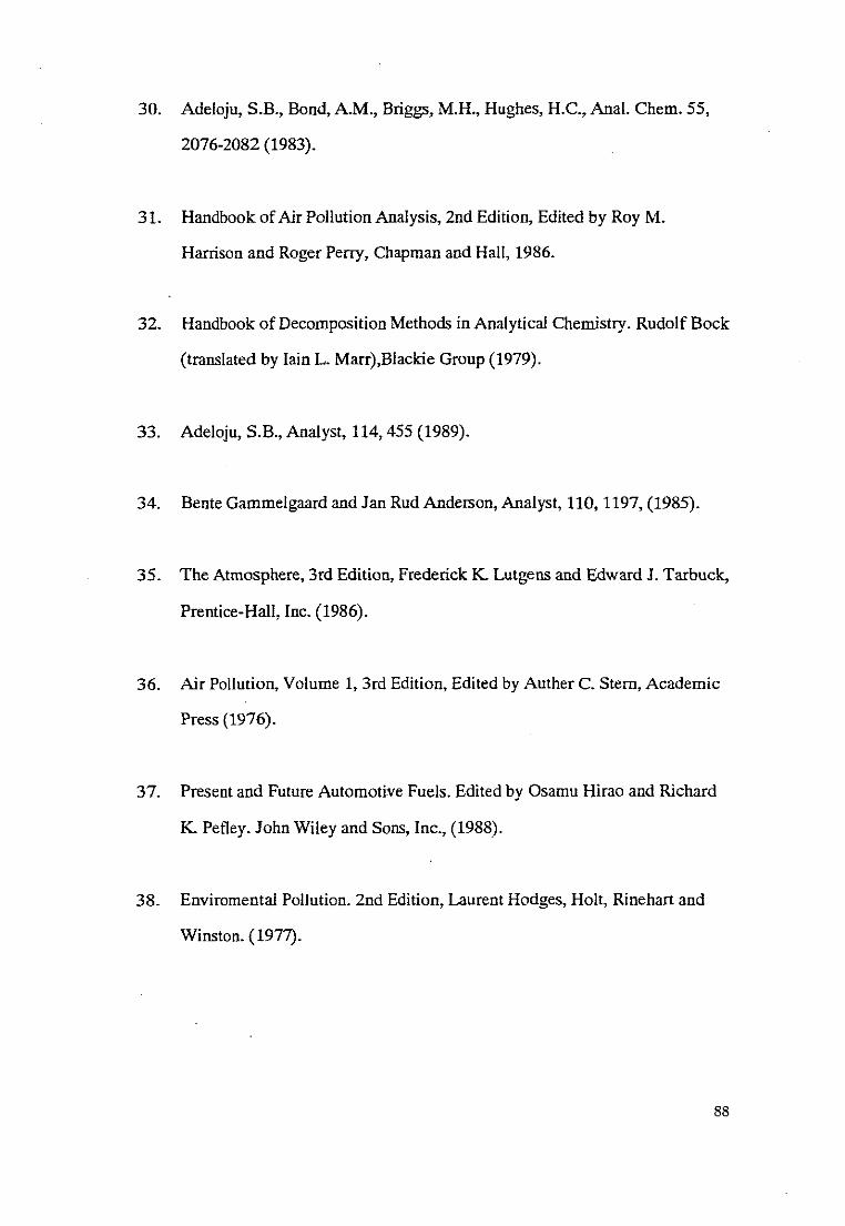
30. Adeloju, S.B., Bond, A.M., Briggs, M.H., Hughes, H.C., Anal. Chem. 55,
2076-2082 (1983).
31. Handbook of Air Pollution Analysis, 2nd Edition, Edited by Roy M.
Harrison and Roger Perry, Chapman and Hall, 1986.
32. Handbook of Decomposition Methods in Analytical Chemistry. Rudolf Bock
(translated by lain L. Marr),Blackie Group (1979).
33. Adeloju, S.B., Analyst, 114,455 (1989).
34. Bente Gammelgaard and Jan Rud Anderson, Analyst, 110, 1197, (1985).
35. The Atmosphere, 3rd Edition, Frederick K. Lutgens and Edward J. Tarbuck,
Prentice-Hall, Inc. (1986).
36. Air Pollution, Volume 1, 3rd Edition, Edited by Auther C. Stern, Academic
Press (1976).
37. Present and Future Automotive Fuels. Edited by Osamu Hirao and Richard
K. Pefley. John Wiley and Sons, Inc., (1988).
38. Enviromental Pollution. 2nd Edition, Laurent Hodges, Holt, Rinehart and
Winston. (1977).
88
Top Related