


Languages
Pages
Legal


Main elements, Cells, Frequency Reuse, Capacity, …
2

• Main Architecture – Cellular Network Architecture – History of Cellular Networks (1st, 2nd, 3rd and 4th Generation) – Operation of Cellular Systems
• Cellular Network Organization – Hexagonal Patterns – Frequency Reuse and Capacity
• Mobility Management – Handoff Strategies
• Traffic Engineering
3

u 1G: analog systems à not in use anymore"u 2G: GSM (introduced in 1992): FDMA/TDMA (900
and 1800MHz)"² 2.5G: with GPRS: packet switching, extended to E-GPRS
(nicknamed EDGE)"u 3G: UMTS (introduced in 2002): CDMA (2100 MHz)"
² 3.5G: with HSPDA (up to 14.4Mb/s); with HSPA+ (up to 84Mb/s) "
u 4G: LTE (being introduced in 2013): OFDMA (800 and 2600MHz, then technology neutrality); up to 100Mb/s"
• GPRS: General Packet Radio Service"• HSPDA: High Speed Downlink Packet Access"• LTE: Long Term Evolution"
4

Mobile Switching
Center
Public telephone network
Mobile Switching
Center
Components of Cellular Network Architecture
v connects cells to wired tel. net. v manages call setup (more later!) v handles mobility (more later!)
MSC
v covers geographical region v base station (BS) analogous to 802.11 AP v mobile users attach to network through BS v air-interface: physical and link layer protocol between mobile and BS
cell
wired network
5
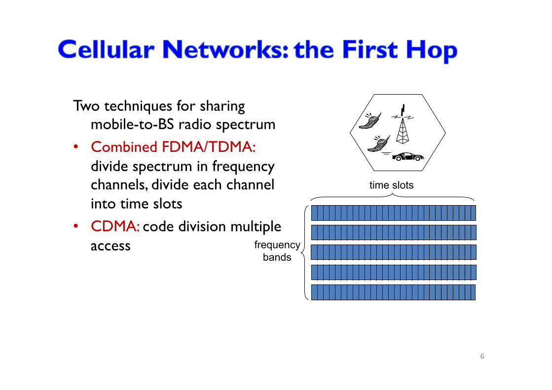
Two techniques for sharing mobile-to-BS radio spectrum
• Combined FDMA/TDMA: divide spectrum in frequency channels, divide each channel into time slots
• CDMA: code division multiple access frequency
bands
time slots
6

BSC BTS
Base transceiver station (BTS)
Base station controller (BSC)
Mobile Switching Center (MSC)
Mobile subscribers
Base station system (BSS)
Legend
2G (voice) Network Architecture
MSC Public telephone network
Gateway MSC
G
7
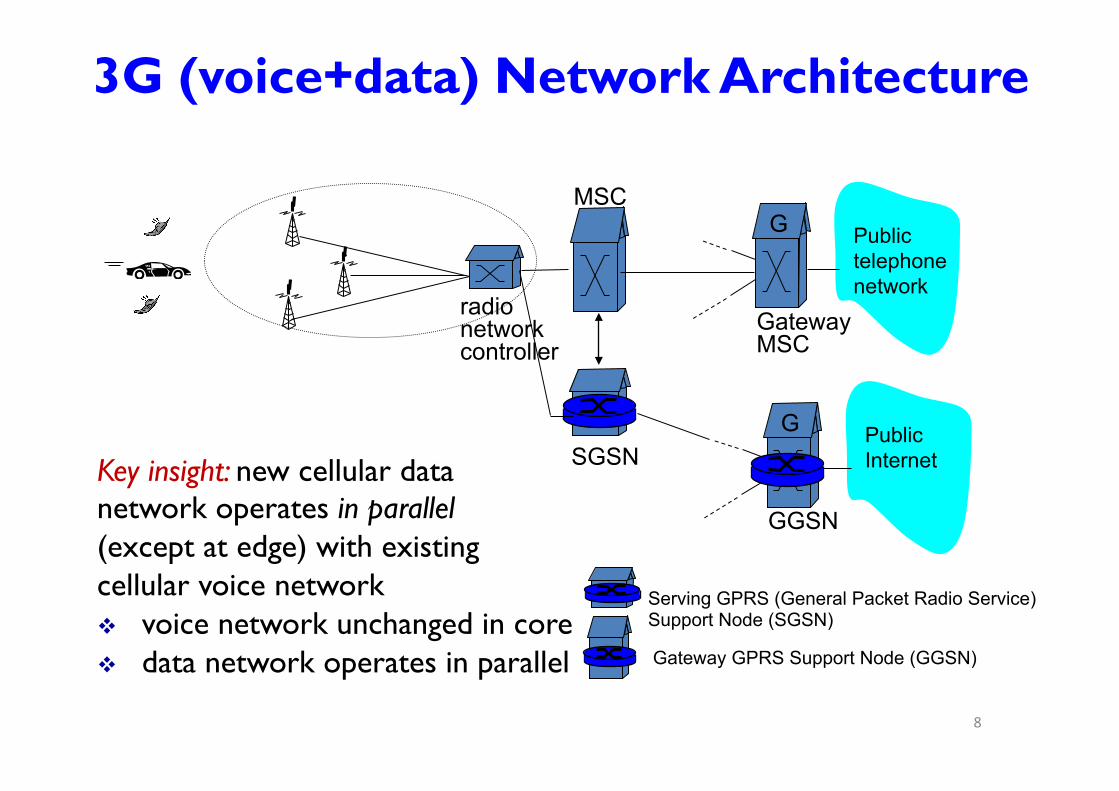
Serving GPRS (General Packet Radio Service) Support Node (SGSN)
Gateway GPRS Support Node (GGSN)
3G (voice+data) Network Architecture
radio network controller
MSC
SGSN
Public telephone network
Gateway MSC
G
Public Internet
GGSN
G
Key insight: new cellular data network operates in parallel (except at edge) with existing cellular voice network v voice network unchanged in core v data network operates in parallel
8
radio network controller
MSC
SGSN
Public telephone network
Gateway MSC
G
Public Internet
GGSN
G
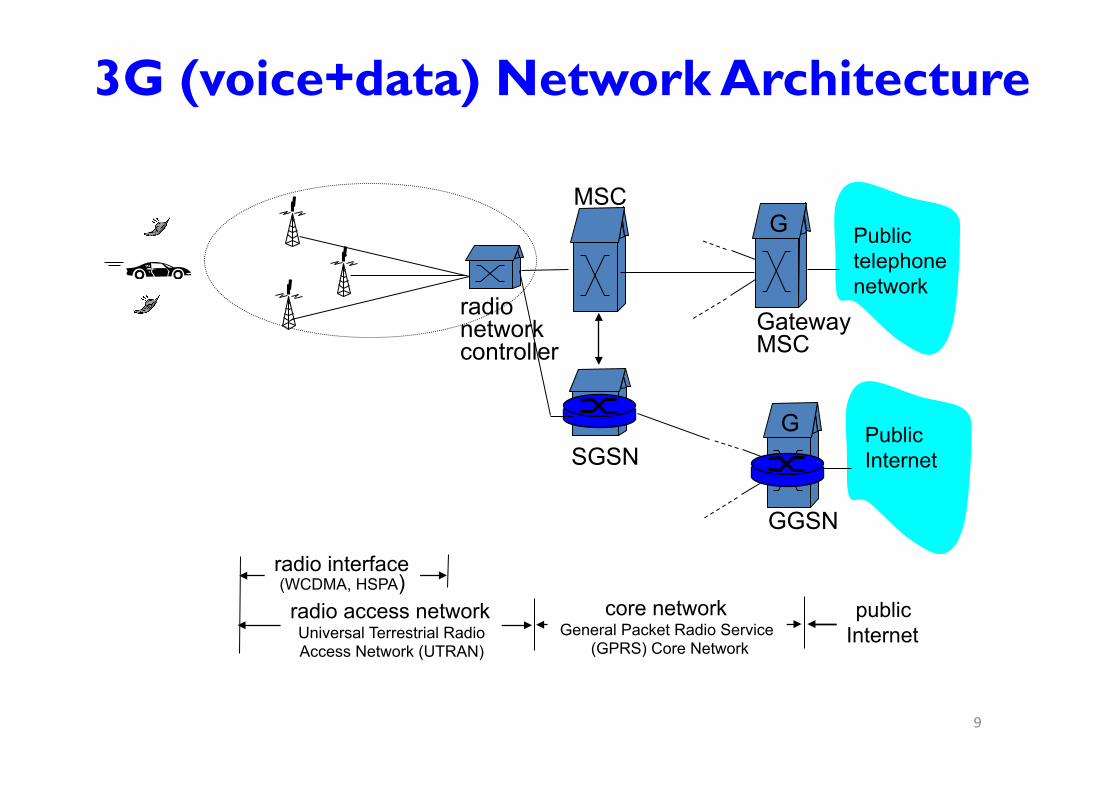
radio access network Universal Terrestrial Radio Access Network (UTRAN)
core network General Packet Radio Service
(GPRS) Core Network
public Internet
radio interface (WCDMA, HSPA)
3G (voice+data) Network Architecture
9

CDMA (IS-95A) GSM
CDMA (IS-95B) cdma 2000 1xEV-DO Rev 0/A/B
UMB 802.20
2G
2.5G
3G 3.5G
4G
GPRS E-GPRS EDGE
HSDPA FDD/TDD
TDMA IS-136
WCDMA FDD/TDD
TD-SCDMA LCR-TDD
HSUPA FDD/TDD
HSPA+ LTE E-UTRA
IEEE 802.16
Fixed WiMAX 802.16d
Mobile WiMAX 802.16e
WiBRO
IEEE 802.11
802.11g
802.11a
802.11g
802.11n
CDMA GSM/UMTS IEEE Cellular IEEE LAN
10
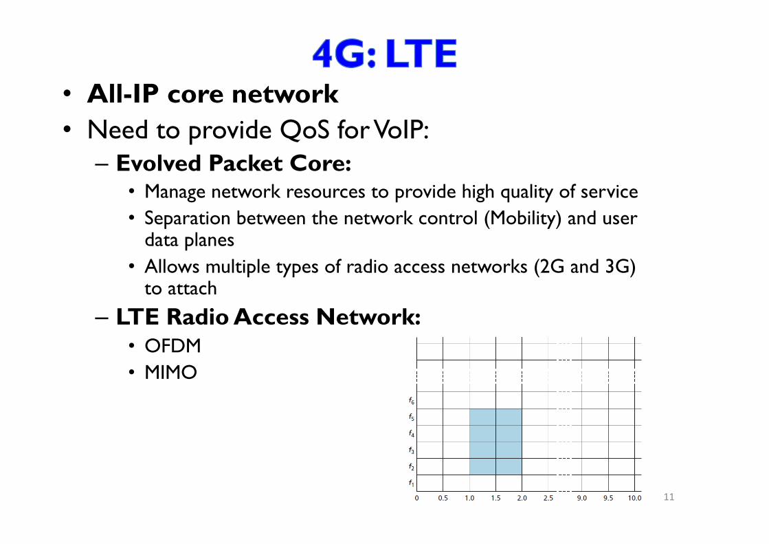
• All-IP core network • Need to provide QoS for VoIP:
– Evolved Packet Core: • Manage network resources to provide high quality of service • Separation between the network control (Mobility) and user
data planes • Allows multiple types of radio access networks (2G and 3G)
to attach – LTE Radio Access Network:
• OFDM • MIMO
11

12

13
In February 2007, the Japanese company NTT DoCoMo tested a 4G communication system prototype with 4×4 MIMO called VSF-OFCDM at 100 Mbit/s while moving, and 1 Gbit/s while stationary. NTT DoCoMo completed a trial in which they reached a maximum packet transmission rate of approximately 5 Gbit/s in the downlink with 12×12.

14

Tune on the strongest signal
BS
MSC Nr: 091x/xxxxxx
15

BS
MSC
Nr: 091x/xxxxxx Nr: 091x/xxxxxx
16

BS
MSC
Nr: 091x/xxxxxx? Nr: 091x/xxxxxx?
Nr: 091x/xxxxxx?
Nr: 091x/xxxxxx?
Note: paging makes sense only over a small area
17
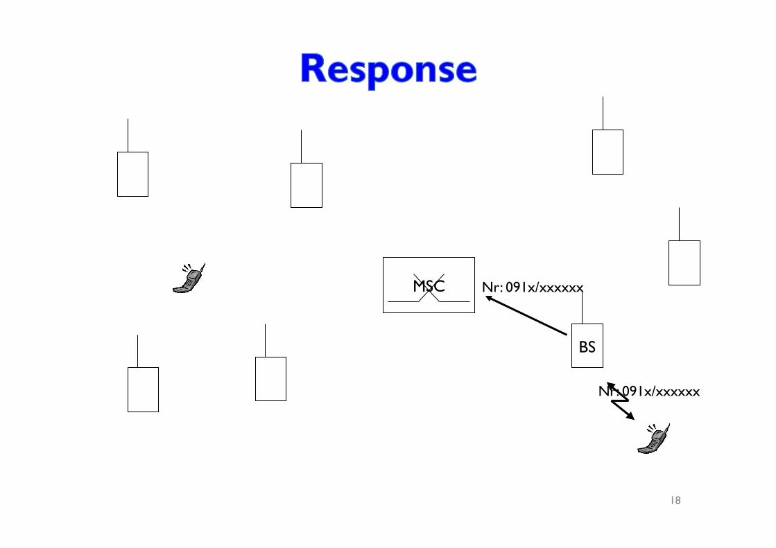
MSC
BS
Nr: 091x/xxxxxx
Nr: 091x/xxxxxx
18

MSC
BS Channel 47
Channel 47 Channel
68
Channel 68
19
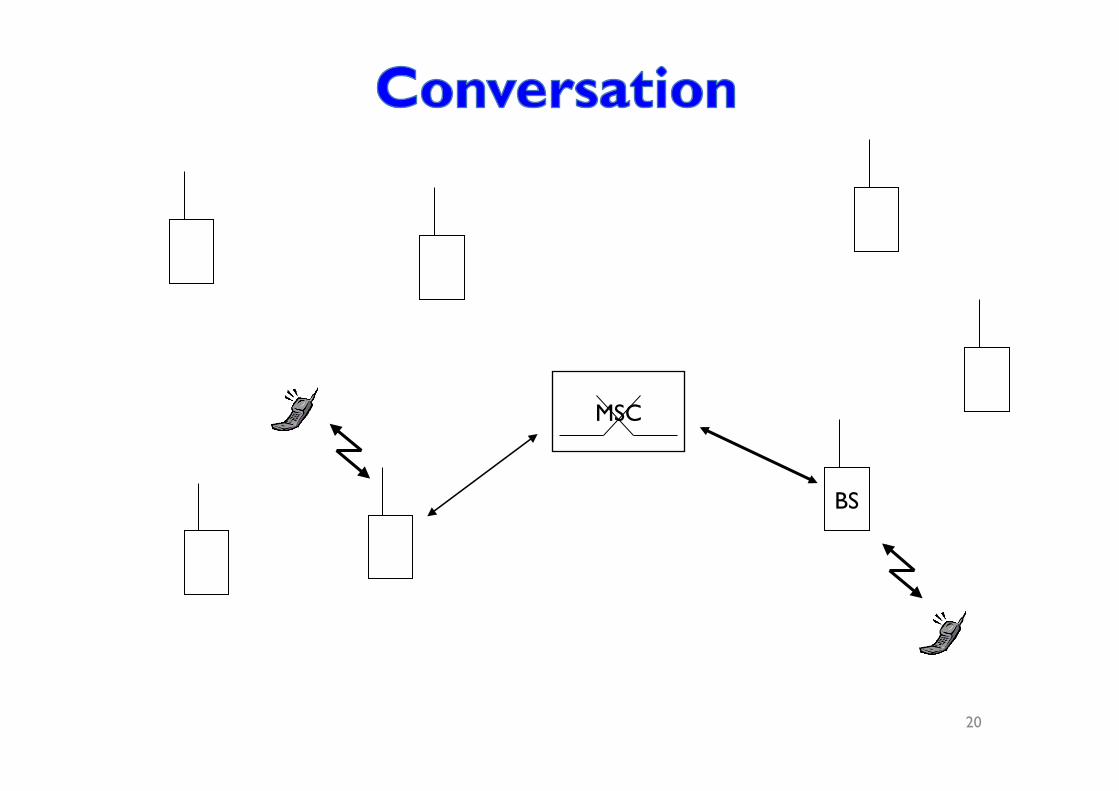
MSC
BS
20

MSC
BS
21

Caller Base Station
Switch Base Station Callee
Periodic registration Periodic registration
Service request Service request
Ring indication Ring indication
Page request Page request Paging broadcast Paging broadcast
Paging response Paging response
Assign Ch. 47 Tune to Ch.47
Assign Ch. 68 Tune to Ch. 68
Alert tone
User response User response Stop ring indication Stop ring indication
22
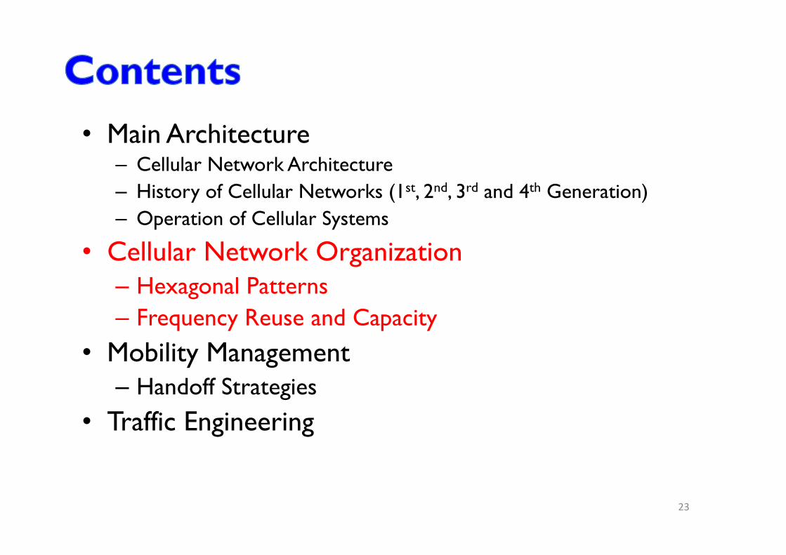
• Main Architecture – Cellular Network Architecture – History of Cellular Networks (1st, 2nd, 3rd and 4th Generation) – Operation of Cellular Systems
• Cellular Network Organization – Hexagonal Patterns – Frequency Reuse and Capacity
• Mobility Management – Handoff Strategies
• Traffic Engineering
23
24
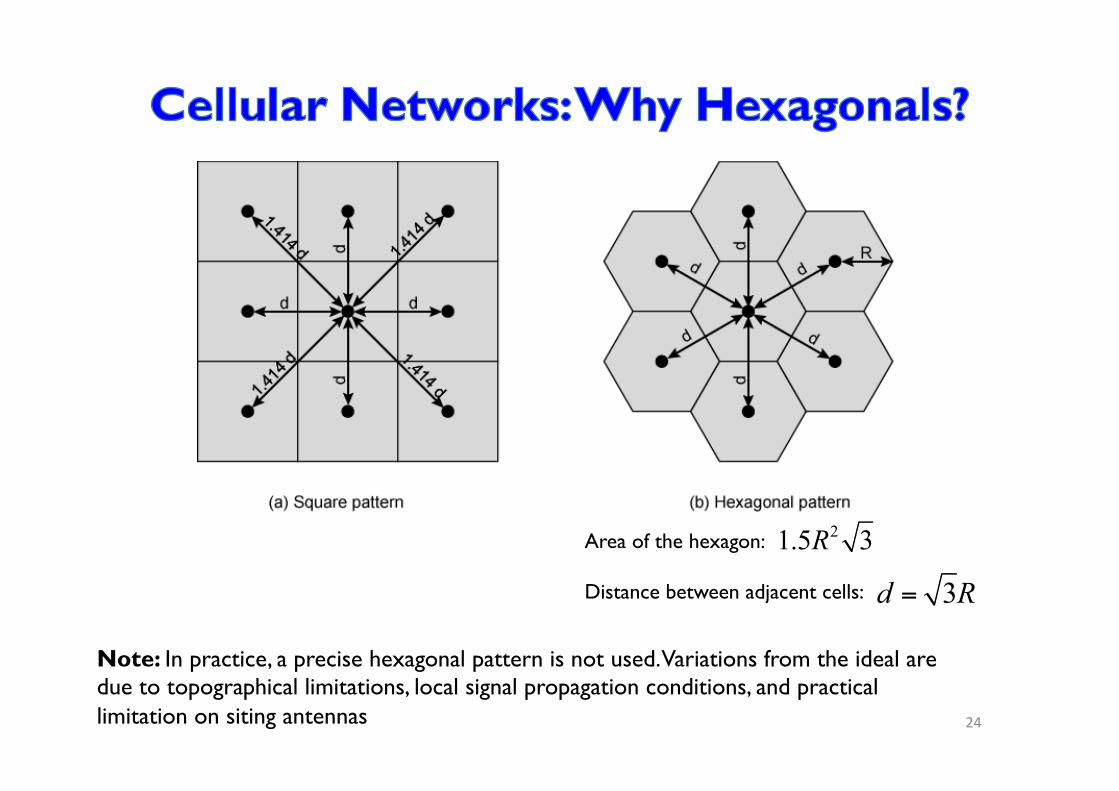
Note: In practice, a precise hexagonal pattern is not used. Variations from the ideal are due to topographical limitations, local signal propagation conditions, and practical limitation on siting antennas
21.5 3RArea of the hexagon: Distance between adjacent cells:
3d R=

q Covered area tesselated in cells o One antenna per cell o Cells are controlled by Mobile Switching
Centers
q A mobile communicates with one (or sometimes two) antennas
q Cells are modeled as hexagons q Cells interfere with each other
q To increase the capacity of the network, increase the number of cells
25
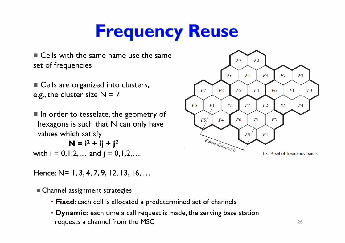
g Channel assignment strategies
• Fixed: each cell is allocated a predetermined set of channels • Dynamic: each time a call request is made, the serving base station requests a channel from the MSC
g Cells with the same name use the same set of frequencies g Cells are organized into clusters, e.g., the cluster size N = 7 g In order to tesselate, the geometry of hexagons is such that N can only have values which satisfy N = i2 + ij + j2
with i = 0,1,2,… and j = 0,1,2,… Hence: N= 1, 3, 4, 7, 9, 12, 13, 16, …
26

N: cluster size
i=2, j=0 i=2, j=1
i=3, j=2 27

28
Define u and v axis as above

29 The cell label:
i = 2

30 The cell label:
i = 3

31

• Sources of interference i Co-channel interference (same frequency)
– A call in a neighboring cell – Other base stations operating in the same frequency band – Non-cellular system leaking energy into the frequency band
i Adjacent channel interference (adjacent frequency) – Another mobile in the same cell
• Consequences of interference i On data channel:
– Crosstalk (voice) – Erroneous data (data transmission)
i On control channel: – Missed/dropped calls
32

33
A
R
D-R
D-R
D
D+R
D+R
D
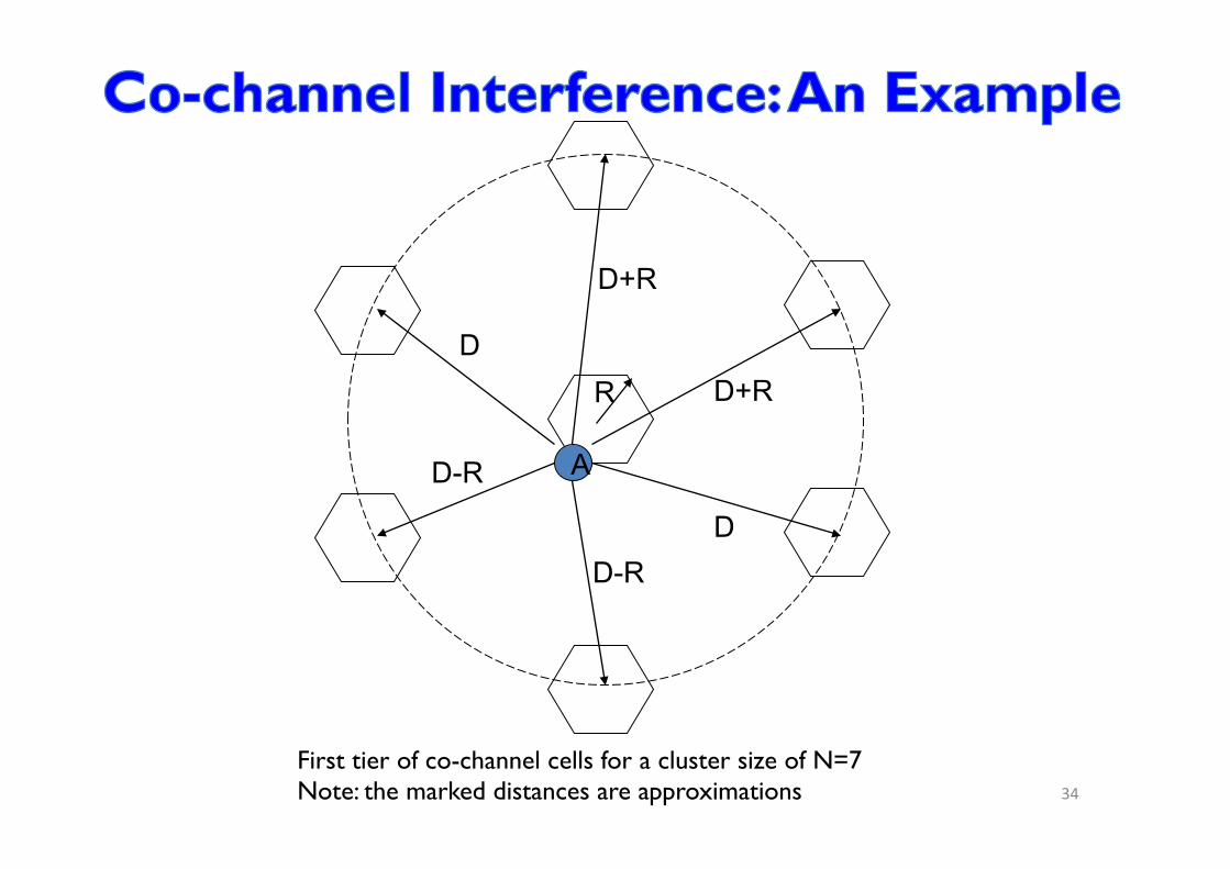
First tier of co-channel cells for a cluster size of N=7 Note: the marked distances are approximations 34

Approximation of the SIR at point A""""""Using the co-channel ratio""""""Numerical example: If N=7, gamma= 4, then q~4.6 and !
CI=
R −γ
2(D − R )−γ + 2D −γ + 2(D + R )−γ
CI≈ 49.56 ≈17.8 dB
35
q = D/R Freq. reuse factor
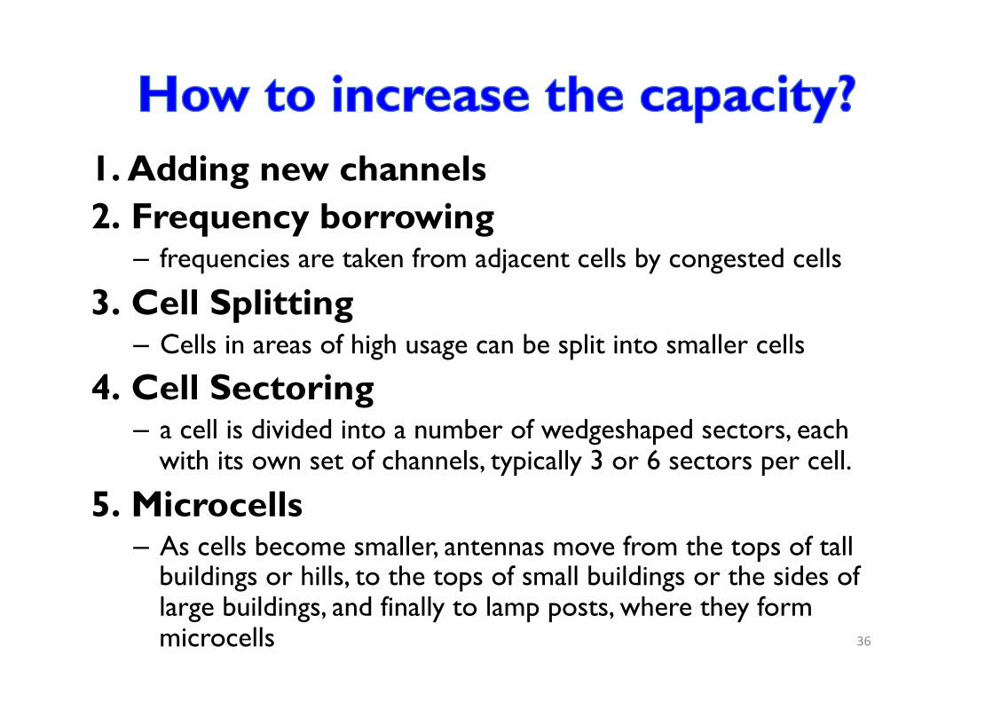
1. Adding new channels 2. Frequency borrowing
– frequencies are taken from adjacent cells by congested cells
3. Cell Splitting – Cells in areas of high usage can be split into smaller cells
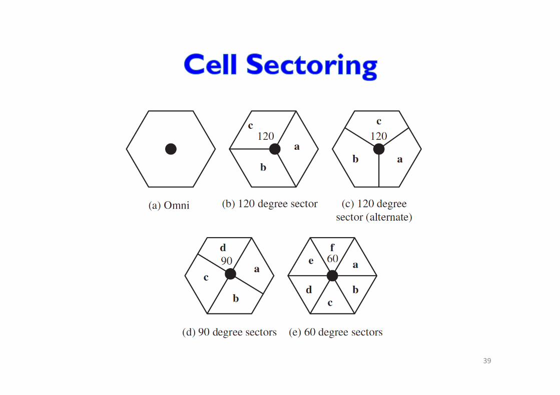
4. Cell Sectoring – a cell is divided into a number of wedgeshaped sectors, each
with its own set of channels, typically 3 or 6 sectors per cell.
5. Microcells – As cells become smaller, antennas move from the tops of tall
buildings or hills, to the tops of small buildings or the sides of large buildings, and finally to lamp posts, where they form microcells 36

37
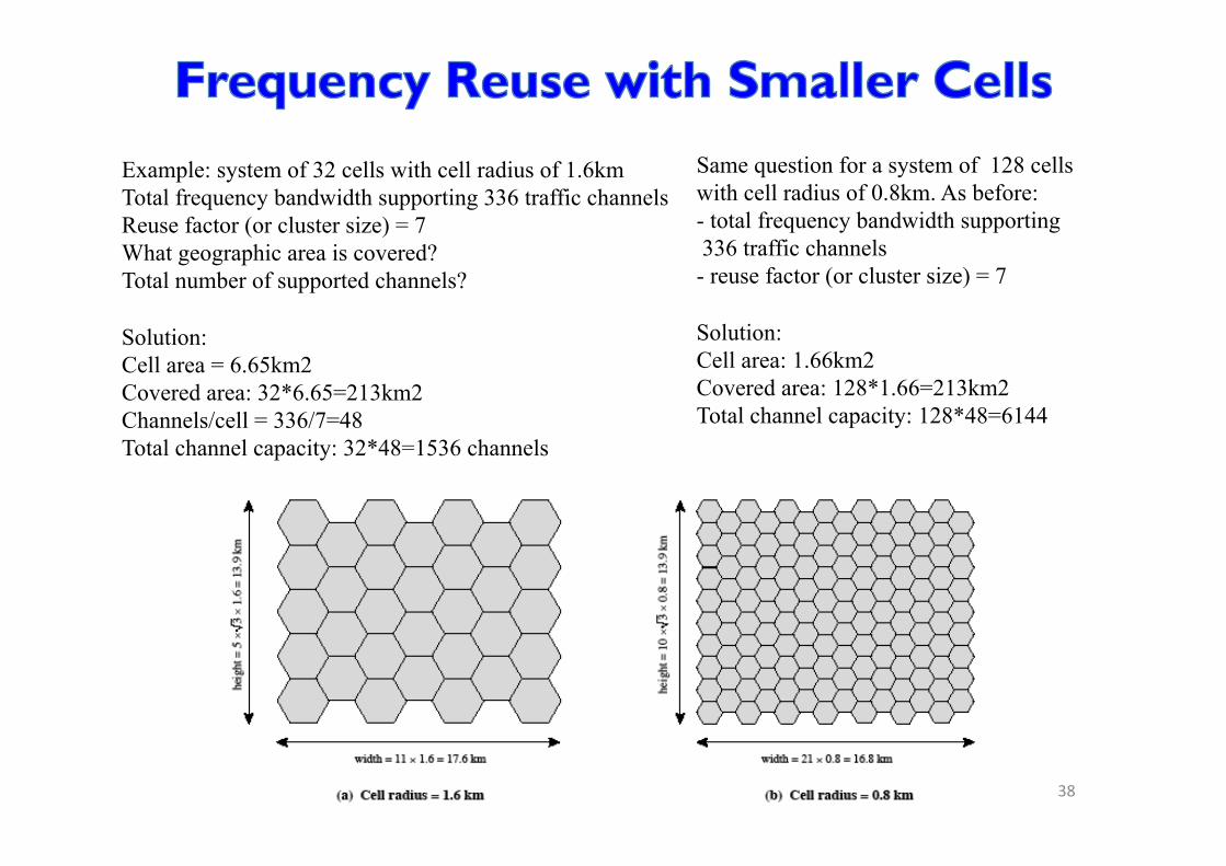
Example: system of 32 cells with cell radius of 1.6km Total frequency bandwidth supporting 336 traffic channels Reuse factor (or cluster size) = 7 What geographic area is covered? Total number of supported channels? Solution: Cell area = 6.65km2 Covered area: 32*6.65=213km2 Channels/cell = 336/7=48 Total channel capacity: 32*48=1536 channels
Same question for a system of 128 cells with cell radius of 0.8km. As before: - total frequency bandwidth supporting 336 traffic channels - reuse factor (or cluster size) = 7
Solution: Cell area: 1.66km2 Covered area: 128*1.66=213km2 Total channel capacity: 128*48=6144
38
39

• Main Architecture – Cellular Network Architecture – History of Cellular Networks (1st, 2nd, 3rd and 4th Generation) – Operation of Cellular Systems
• Cellular Network Organization – Hexagonal Patterns – Frequency Reuse and Capacity
• Mobility Management – Handoff Strategies
• Traffic Engineering
40

Components of Cellular Network Architecture
correspondent
MSC
MSC MSC MSC
MSC
wired public telephone network
different cellular networks, operated by different providers
recall:
41

• home network: network of cellular provider you subscribe to (e.g., Sprint PCS, Verizon) – home location register (HLR): database in home network
containing permanent cell phone #, profile information (services, preferences, billing), information about current location (could be in another network)
• visited network: network in which mobile currently resides – visitor location register (VLR): database with entry for
each user currently in network – could be home network
42

Public switched telephone network
mobile user
home Mobile
Switching Center
HLR home network
visited network
correspondent
Mobile Switching
Center
VLR
GSM: indirect routing to mobile
1 call routed to home network
2
home MSC consults HLR, gets roaming number of mobile in visited network
3
home MSC sets up 2nd leg of call to MSC in visited network
4
MSC in visited network completes call through base station to mobile
43

2. Receive the ID of the LA 3. Compare with stored ID
4. If different, update and ask for registration
Location area 1 (ID = 1) Location area 2 (ID = 2)
• Base stations periodically broadcast the ID of the LA • Users compare their last LA ID with the current ID, and transmits a registration message whenever the ID is different
• When there is an incoming call directed to a user, all cells within its current LA are paged
1. Change LA
5. Inform the HLR of the new LA ID
44

• Temporary Mobile Subscriber identifiers – TMSI – changed after crossing Location Area (LA) border or time-out trigger
LA 0 LA 1
LA 2
LA 3
Pseudo A
Pseudo B
Pseudo C
Pseudo D
45

Mobile Switching
Center
VLR
old BSS new BSS
old routing
new routing
GSM: Handoff with Common MSC
• handoff goal: route call via new base station (without interruption)
• reasons for handoff: – stronger signal to/from new BSS
(continuing connectivity, less battery drain)
– load balance: free up channel in current BSS
– GSM doesn’t mandate why to perform handoff (policy), only how (mechanism)
• handoff initiated by old BSS
46

Mobile Switching
Center
VLR
old BSS
1
3
2 4
5 6
7 8
new BSS
1. old BSS informs MSC of impending handoff, provides list of 1+ new BSSs
2. MSC sets up path (allocates resources) to new BSS
3. new BSS allocates radio channel for use by mobile
4. new BSS signals MSC, old BSS: ready 5. old BSS tells mobile: perform handoff to new
BSS 6. mobile, new BSS signal to activate new
channel 7. mobile signals via new BSS to MSC: handoff
complete. MSC reroutes call 8 MSC-old-BSS resources released
GSM: Handoff with Common MSC
47

BS1 BS2
A B
t
Received signal level
Level at B
Level at which handover is made (call transferred to BS2)
48

Hard: Communicate with one cell at a time Soft: Communicate with two cells simultaneously g TDMA & FDMA: Hard
– Could technically use soft handover, but would be costly as it would require multiple parallel radio modules
g CDMA: Soft
– Needed to avoid near-far problem (i.e., Detect weaker signal amongst strong signals)
49
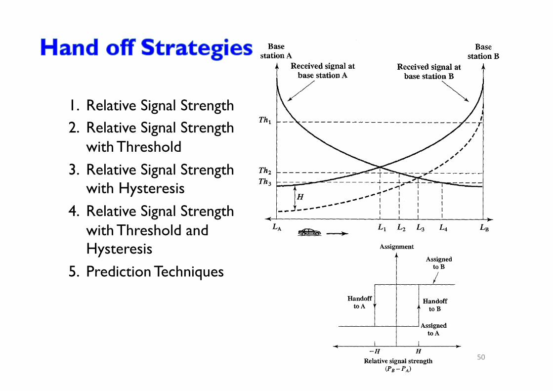
1. Relative Signal Strength 2. Relative Signal Strength
with Threshold 3. Relative Signal Strength
with Hysteresis 4. Relative Signal Strength
with Threshold and Hysteresis
5. Prediction Techniques
50

home network
Home MSC
PSTN
correspondent
MSC anchor MSC
MSC MSC
(a) before handoff
GSM: Handoff between MSCs
• Anchor MSC: first MSC visited during call - call remains routed through anchor MSC
• New MSCs add on to end of MSC chain as mobile moves to new MSC - optional path minimization step to shorten multi-MSC chain
51

home network
Home MSC
PSTN
correspondent
MSC anchor MSC
MSC MSC
(b) after handoff
§ Anchor MSC: first MSC visited during call - call remains routed through anchor MSC
§ New MSCs add on to end of MSC chain as mobile moves to new MSC - optional path minimization step to shorten multi-MSC chain
GSM: Handoff between MSCs
52

• Main Architecture – Cellular Network Architecture – History of Cellular Networks (1st, 2nd, 3rd and 4th Generation) – Operation of Cellular Systems
• Cellular Network Organization – Hexagonal Patterns – Frequency Reuse and Capacity
• Mobility Management – Handoff Strategies
• Traffic Engineering
53

• Consider a cell – has L potential subscribers (L mobile units) – Able to handle N simultaneous users (capacity of N
channels)
• If L <= N è The system is nonblocking system
• If L > N è The system is blocking
54
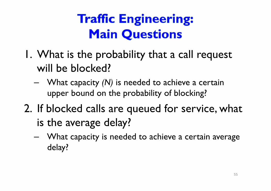
1. What is the probability that a call request will be blocked?
– What capacity (N) is needed to achieve a certain upper bound on the probability of blocking?
2. If blocked calls are queued for service, what is the average delay?
– What capacity is needed to achieve a certain average delay?
55

56
A = λ ⋅ h [Erlangs]
where h = The mean holding time per successful call λ = The mean rate of calls (connection requests) attempted per unit time N = Number of Servers
PrBlocking = Pr("call dropped because line busy") = Erlang-B(A ,N ) = A N
N ! A i
i !
!
"#
$
%&
i =0
N∑
57
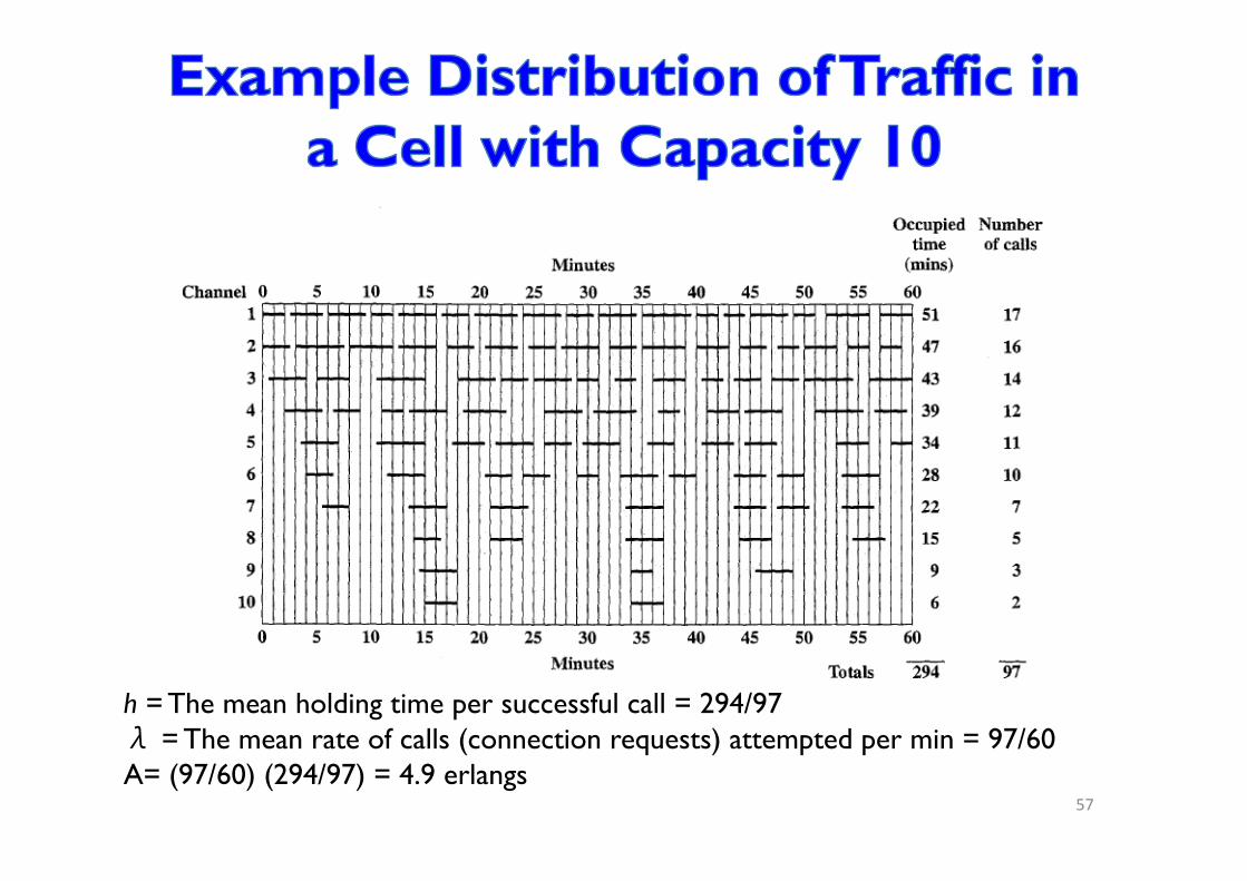
h = The mean holding time per successful call = 294/97 λ = The mean rate of calls (connection requests) attempted per min = 97/60 A= (97/60) (294/97) = 4.9 erlangs
58
Top Related