Download - Module 3 - UCSC Directory of individual web sitesdgbonett/docs/psyc214a/214AMod3.pdf · D.G. Bonett (3/2018) 3 which can be expressed more compactly as cov(e) = I n ⨂𝚺 where

D.G. Bonett (8/2018)

1

Module 3

Covariance Pattern Models for Repeated Measures Designs

Recall from Module 2 that the GLM can be expressed as

𝑦𝑖 = 𝛽0 + 𝛽1𝑥1𝑖 + 𝛽2𝑥2𝑖 + … + 𝛽𝑞𝑥𝑞𝑖 + 𝑒𝑖

where 𝑦𝑖 is the response variable score for participant i and 𝑒𝑖 is the prediction

error for participant i. In a random sample of n participants, there are n prediction

errors (𝑒1, 𝑒2, … , 𝑒𝑛). The GLM assumes that the n prediction errors are

uncorrelated. This assumption is reasonable in most applications because each

prediction error corresponds to a different participant, and it usually easy to design

a study such that no participant influences the response of any other participant.

In a repeated measures design, each participant provides r ≥ 2 responses. The

longitudinal design, the pretest-posttest design, and the within-subjects

experimental design are all special cases of the repeated measured design. In a

longitudinal design, the response variable for each participant is measured on two

or more occasions. In a pretest-posttest design, the response variable is measured

on one or more occasions prior to treatment and then on one or more occasions

following treatment. In a within-subjects experimental design, the response

variable for each participant is measured under all treatment conditions (usually

in counterbalanced order).

In a study with repeated measurements, the relation between the response variable

(y) and q predictor variables (𝑥1, 𝑥2, … 𝑥𝑞) for one randomly selected person can be

represented by the following covariance pattern model (CPM)

𝑦𝑖𝑗 = 𝛽0 + 𝛽1𝑥1𝑖𝑗 + … + 𝛽𝑠𝑥𝑠𝑖𝑗 + 𝛽𝑠+1𝑥𝑠+1𝑖 … + 𝛽𝑞𝑥𝑞𝑖 + 𝑒𝑖𝑗

where i = 1 to n and j = 1 to r. Note that the i subscript specifies a particular

participant and the j subscript specifies a particular occasion. Note also that

predictor variables 𝑥𝑠+1 to 𝑥𝑞 do not have a j subscript, as in a GLM, and describe

differences among the participants. These predictor variables are called time-

invariant predictor variables because their values will vary across participants but

remain constant over the r repeated measurements.

Predictor variables 𝑥1 to 𝑥𝑠 in the CPM have both an i subscript and a j subscript.

These predictor variables are called time-varying predictor variables because they

can vary over time and across participants. A CPM can have all time-invariant


2

predictors, all time-varying predictors, or a combination of time-invariant and

time-varying predictors.

The time-invariant and time-varying predictor variables can be indicator variables,

fixed or random quantitative variables, or any combination of indicator and

quantitative variables. The predictor variables can be squared variables to describe

quadratic effects or product variables to describe interaction effects. A product

variable can be a product of two time-varying predictor variables, a product of two

time-invariant predictor variables, or a product of a time-invariant predictor

variable and a time varying predictor variables.

The CPM has n x r prediction errors (𝑒11, … 𝑒1𝑟 , 𝑒21, … 𝑒2𝑟 , 𝑒𝑛1 … 𝑒𝑛𝑟). The r

prediction errors for each participant in the CPM are assumed to be correlated and

possibly also have unequal variances. The prediction errors for different

participants are assumed to be uncorrelated as in the GLM. The variances and

covariances of the prediction errors in a CPM can be represented by a prediction

error covariance matrix as described below.

Prediction Error Covariance Matrices

A prediction error covariance matrix is a symmetric matrix with variances of the

prediction errors in the diagonal elements and covariances among pairs of

prediction errors in the off-diagonal elements. In the GLM where the n prediction

errors are assumed to be uncorrelated and have the same variance, the prediction

error covariance matrix for the n x 1 vector of prediction errors (e) has the

following diagonal structure

cov(e) = [

𝜎2 0 ⋯ 00 𝜎2 … 0⋮ ⋮ ⋮0 0 ⋯ 𝜎2

]

which can be expressed more compactly as cov(e) = 𝜎2𝐈𝑛.

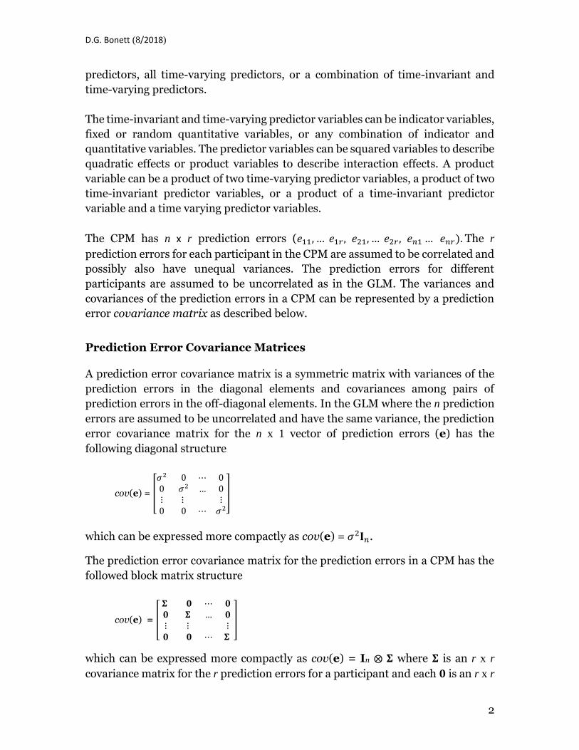
The prediction error covariance matrix for the prediction errors in a CPM has the

followed block matrix structure

cov(e) = [

𝚺 𝟎 ⋯ 𝟎𝟎 𝚺 … 𝟎⋮ ⋮ ⋮𝟎 𝟎 ⋯ 𝚺

]

which can be expressed more compactly as cov(e) = In ⨂ 𝚺 where 𝚺 is an r x r

covariance matrix for the r prediction errors for a participant and each 𝟎 is an r x r


3

matrix of zeros. The r x r covariance matrix (𝚺) is usually assumed to be identical

across the n participants.

The r variances and the r(r – 1)/2 covariances of the r prediction errors for

participant i [𝑒𝑖1, … , 𝑒𝑖𝑟] can be summarized in an r × r covariance matrix denoted

as 𝚺. For example, the covariance matrix for r = 3 is

𝚺 = [𝜎1

2

𝜎12

𝜎13

𝜎12

𝜎22

𝜎23

𝜎13

𝜎23

𝜎32]

where 𝜎12 is the prediction error variance for occasion 1, 𝜎2

2 is the prediction error

variance for occasion 2, 𝜎32 is the prediction error variance for occasion 3, 𝜎12 is the

covariance of prediction errors for occasions 1 and 2, 𝜎13 is the covariance of

prediction errors for occasions 1 and 3, and 𝜎23 is the covariance of prediction

errors for occasions 2 and 3.

The above covariance matrix is referred to as an unstructured covariance matrix

because there are no assumptions made regarding the values of the variances or

covariances. An unstructured covariance matrix requires the estimation of r

variances and r(r – 1)/2 covariances, or a total of r(r + 1)/2 parameters.

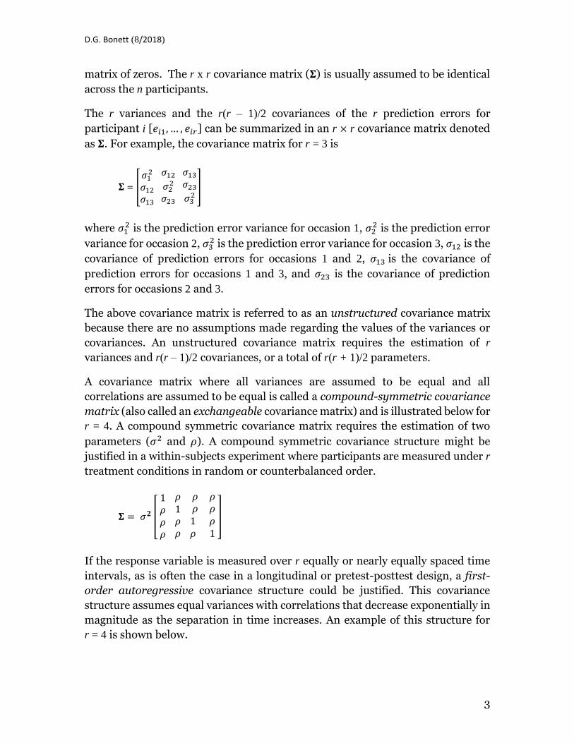
A covariance matrix where all variances are assumed to be equal and all

correlations are assumed to be equal is called a compound-symmetric covariance

matrix (also called an exchangeable covariance matrix) and is illustrated below for

r = 4. A compound symmetric covariance matrix requires the estimation of two

parameters (𝜎2 and 𝜌). A compound symmetric covariance structure might be

justified in a within-subjects experiment where participants are measured under r

treatment conditions in random or counterbalanced order.

𝚺 = 𝜎𝟐 [

1𝜌𝜌𝜌

𝜌 1 𝜌𝜌

𝜌 𝜌 𝜌 𝜌 1 𝜌 𝜌 1

]

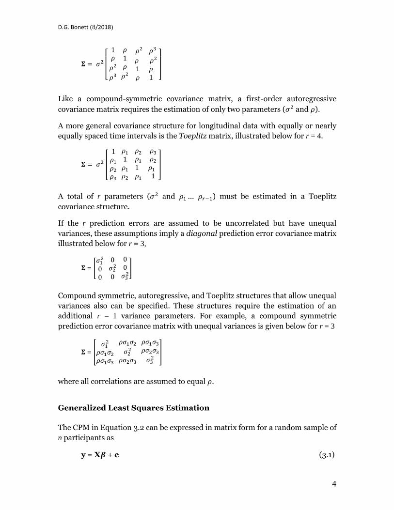
If the response variable is measured over r equally or nearly equally spaced time

intervals, as is often the case in a longitudinal or pretest-posttest design, a first-

order autoregressive covariance structure could be justified. This covariance

structure assumes equal variances with correlations that decrease exponentially in

magnitude as the separation in time increases. An example of this structure for

r = 4 is shown below.


4

𝚺 = 𝜎𝟐

[

1𝜌

𝜌2

𝜌3

𝜌 1 𝜌

𝜌2

𝜌2 𝜌3

𝜌 𝜌2

1 𝜌𝜌 1

]

Like a compound-symmetric covariance matrix, a first-order autoregressive

covariance matrix requires the estimation of only two parameters (𝜎2 and 𝜌).

A more general covariance structure for longitudinal data with equally or nearly

equally spaced time intervals is the Toeplitz matrix, illustrated below for r = 4.

𝚺 = 𝜎𝟐 [

1𝜌1

𝜌2

𝜌3

𝜌1

1 𝜌1

𝜌2

𝜌2 𝜌3

𝜌1 𝜌2

1 𝜌1

𝜌1 1

]

A total of r parameters (𝜎2 and 𝜌1 … 𝜌𝑟−1) must be estimated in a Toeplitz

covariance structure.

If the r prediction errors are assumed to be uncorrelated but have unequal

variances, these assumptions imply a diagonal prediction error covariance matrix

illustrated below for r = 3,

𝚺 = [𝜎1

2

00

0𝜎2

2

0

00𝜎3

2]

Compound symmetric, autoregressive, and Toeplitz structures that allow unequal

variances also can be specified. These structures require the estimation of an

additional r – 1 variance parameters. For example, a compound symmetric

prediction error covariance matrix with unequal variances is given below for r = 3

𝚺 = [𝜎1

2

𝜌𝜎1𝜎2

𝜌𝜎1𝜎3

𝜌𝜎1𝜎2

𝜎22

𝜌𝜎2𝜎3

𝜌𝜎1𝜎3

𝜌𝜎2𝜎3

𝜎32

]

where all correlations are assumed to equal 𝜌.

Generalized Least Squares Estimation

The CPM in Equation 3.2 can be expressed in matrix form for a random sample of

n participants as

y = X𝜷 + e (3.1)


5

where y is an nr x 1 vector of observations, X is a nr x q + 1 design matrix, 𝜷 is a

q + 1 x 1 vector of parameters (containing one y-intercept and q slope coefficients),

and e is nr x 1 vector of prediction errors.

The OLS estimate of 𝜷 (Equation 2.19) is appropriate if the prediction errors are

uncorrelated and have a common variance (i.e., cov(e) = 𝜎𝑒2𝐈𝑛). In the CPM, the

prediction error covariance matrix is cov(e) = In ⨂ 𝚺. Let �̂�= In ⨂ �̂� where �̂� is the

sample estimate of 𝚺. The sample estimate of 𝚺 is obtained by computing an OLS

estimate of 𝜷 (Equation 2.19) and the vector of estimated prediction errors using

Equation 2.20. The sample variances and covariances are then computed from

these estimated prediction errors. When the prediction errors are not assumed to

be uncorrelated or have equal variances, 𝜷 in Equation 3.1 is usually estimated

using generalized least squares (GLS) rather than OLS. The GLS estimate of 𝜷 is

�̂�GLS = (𝐗′�̂�−1𝐗)−1𝐗′�̂�−1𝐲. (3.2)

The GLS estimate of 𝜷 can be used to obtained a revised estimate of the estimated

prediction errors and a revised estimate of 𝚺 is computed from these revised

prediction errors. Equation 3.2 is recomputed using the revised �̂�= In ⨂ �̂�. This

process is continued until the GLS estimate of 𝜷 stabilizes.

The covariance matrix of �̂�GLS is

cov(�̂�GLS) = (𝐗′�̂�−1𝐗)−1 (3.3)

and the standard error of a particular slope estimate (𝛽𝑘) is equal to the square root of the kth diagonal element in Equation 3.3. An approximate 100(1 – 𝛼)% confidence interval for 𝛽𝑘 is given below.

�̂�𝑘 ± 𝑡𝛼/2;𝑑𝑓𝑆𝐸�̂�𝑘 (3.4)

The recommended df for Equation 3.4 uses a Satterthwaite df that has a

complicated formula. SAS and SPSS can be used to compute Equation 3.4 with a

Satterthwaite df.

A confidence interval for 𝛽𝑘 can be used to test H0: 𝛽𝑘 = b, where b is some numeric

value specified by the researcher. A directional two-sided test can be used to choose

H1: 𝛽𝑘 > b or H2: 𝛽𝑘 < b, or declare the results to be inconclusive.

Unlike the GLM, confidence interval methods are not currently available for

standardized slopes or semi-partial correlations in the CPM. Therefore, it is

especially important for the researcher to have a clear understanding of the metrics


6

of all variables in the CPM in order to properly interpret the scientific meaning or

practical implications of a confidence interval for 𝛽𝑘.

Centering the Predictor Variables

Consider a simple CPM that has only time (𝑥1) as a predictor variable

𝑦𝑖𝑗 = 𝛽0 + 𝛽1𝑥1𝑖𝑗 + 𝑒𝑖𝑗 (Model 1)

where 𝛽1 is the slope of the line relating 𝑥1 to y and 𝛽0 is the y-intercept. Suppose

𝑥1 was coded 1, 2, 3, 4, and 5 to represent five possible weeks when a participant

could be measured. With 𝑥1 coded this way, 𝛽0 describes the predicted y-score for

𝑥1 = 0 which would correspond to one week prior to the start of the study. If 𝑥1 had

instead been baseline centered so that 𝑥1 was coded 0, 1, 2, 3, and 4, then 𝛽0 would

describe the predicted y-score for the first week of the study. The time variable also

could be mean centered. If 𝑥1 is coded -2, -1, 0, 1, and 2 then 𝛽0 would describe the

predicted y-score for the third week of the study.

It is usually a good idea to mean center all time-invariant predictor variables.

Consider the following CPM that has one time-invariant predictor variable

𝑦𝑖𝑗 = 𝛽0 + 𝛽1𝑥1𝑖𝑗+ 𝛽2𝑥2𝑖 + 𝑒𝑖𝑗 (Model 2)

where 𝑥2𝑖 is the time-invariant score for participant i. As an example, if 𝑥1 is

baseline centered and 𝑥2𝑖 is the ACT score for participant i then 𝛽0 describes the

predicted y-score at week 1 for participants with an ACT score of 0. This y-intercept

is not meaningful because an ACT score of 0 is impossible. However, if the ACT

scores are mean centered, then 𝛽0 describes the predicted y-score at week 1 for

participants with an average ACT score. If a product of two time-invariant

predictor variables is included in the model to assess an interaction effect, the

time-invariant predictor variables should be mean centered before computing

product variable.

Time-varying predictor variables should be person centered rather than mean

centered. Consider the following CPM that adds a time-varying predictor variable

to Model 1

𝑦𝑖𝑗 = 𝛽0 + 𝛽1𝑥1𝑖𝑗 + 𝛽2𝑥2𝑖𝑗 + 𝑒𝑖𝑗 (Model 3)


7

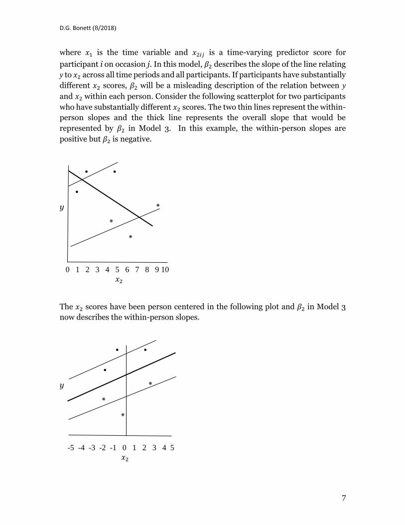
where 𝑥1 is the time variable and 𝑥2𝑖𝑗 is a time-varying predictor score for

participant i on occasion j. In this model, 𝛽2 describes the slope of the line relating

y to 𝑥2 across all time periods and all participants. If participants have substantially

different 𝑥2 scores, 𝛽2 will be a misleading description of the relation between y

and 𝑥2 within each person. Consider the following scatterplot for two participants

who have substantially different 𝑥2 scores. The two thin lines represent the within-

person slopes and the thick line represents the overall slope that would be

represented by 𝛽2 in Model 3. In this example, the within-person slopes are

positive but 𝛽2 is negative.

. .

.

y *

*

*

0 1 2 3 4 5 6 7 8 9 10

𝑥2

The 𝑥2 scores have been person centered in the following plot and 𝛽2 in Model 3

now describes the within-person slopes.

. .

.

y *

*

*

-5 -4 -3 -2 -1 0 1 2 3 4 5

𝑥2


8

When a time-varying predictor variable (𝑥2) has been person centered, the slope

coefficient for 𝑥2 describes the within-person relation between y and 𝑥2. Some of

the variability in y can usually be predicted by between-person differences in 𝑥2,

but these between-person differences are lost when 𝑥2 is person centered. This lost

information can be recovered by simply adding another predictor variable to the

model that represents the mean time-varying predictor score for each participant

as shown below in Model 4

𝑦𝑖𝑗 = 𝛽0 + 𝛽1𝑥1𝑖𝑗 + 𝛽2𝑥2𝑖𝑗 + 𝛽3𝑥3𝑖 + 𝑒𝑖𝑗 (Model 4)

where 𝑥2𝑖𝑗 is the person-centered time-varying predictor variable score for

participant i on occasion j and 𝑥3𝑖 is the mean time-varying predictor score for

participant i. Note that 𝑥3 is a time-invariant predictor variable. In Model 4, 𝛽2

describes the slope of the line relating y to 𝑥1 across time and within persons and

𝛽3 describes the slope of the line relating y to 𝑥2 across persons.

To illustrate the computation of 𝑥2 and 𝑥3 in Model 4, considered the following

hypothetical data for the first two participants where 𝑥1 is the time variable

(baseline centered) and 𝑥2 is a time-varying predictor variable. Participant 1 was

measured on three occasions and participant 2 was measured on four occasions.

Participant y x1 x2

1 15 0 7

1 19 1 9

1 22 2 11

2 23 0 16

2 27 1 19

2 34 2 25

2 35 3 28

The mean of the 𝑥2 scores for participant 1 is (7 + 9 + 11)/3 = 9 and the mean of the

𝑥2 scores for participant 2 is (16 + 19 + 25 + 28)/4 = 22. Subtract 9 from the 𝑥2 scores

for participant 1 and subtract 22 from the 𝑥2 scores for participant 2. The person

centered 𝑥2 scores are given below along with a new time-invariant variable (𝑥3)

that has the person means of 𝑥2.

Participant y x1 x2 x3

1 15 0 -2 9

1 19 1 0 9

1 22 2 2 9

2 23 0 -6 22

2 27 1 -3 22

2 34 2 3 22

2 35 3 6 22


9

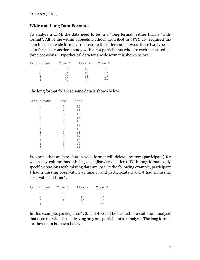
Wide and Long Data Formats

To analyze a CPM, the data need to be in a "long format" rather than a "wide

format". All of the within-subjects methods described in PSYC 204 required the

data to be in a wide format. To illustrate the difference between these two types of

data formats, consider a study with n = 4 participants who are each measured on

three occasions. Hypothetical data for a wide format is shown below.

Participant Time 1 Time 2 Time 3

1 10 14 15

2 15 18 17

3 12 13 19

4 14 20 22

The long format for these same data is shown below.

Participant Time Score

1 1 10

1 2 14

1 3 15

2 1 15

2 2 18

2 3 17

3 1 12

3 2 13

3 3 19

4 1 14

4 3 20

4 3 22

Programs that analyze data in wide format will delete any row (participant) for

which any column has missing data (listwise deletion). With long format, only

specific occasions with missing data are lost. In the following example, participant

1 had a missing observation at time 2, and participants 2 and 4 had a missing

observation at time 1.

Participant Time 1 Time 2 Time 3

1 10 -- 15

2 -- 18 17

3 12 13 19

4 -- 20 22

In this example, participants 1, 2, and 4 would be deleted in a statistical analysis

that used the wide format leaving only one participant for analysis. The long format

for these data is shown below.


10

Participant Time Score

1 1 10

1 3 15

2 2 18

2 3 17

3 1 12

3 2 13

3 3 19

4 3 20

4 3 22

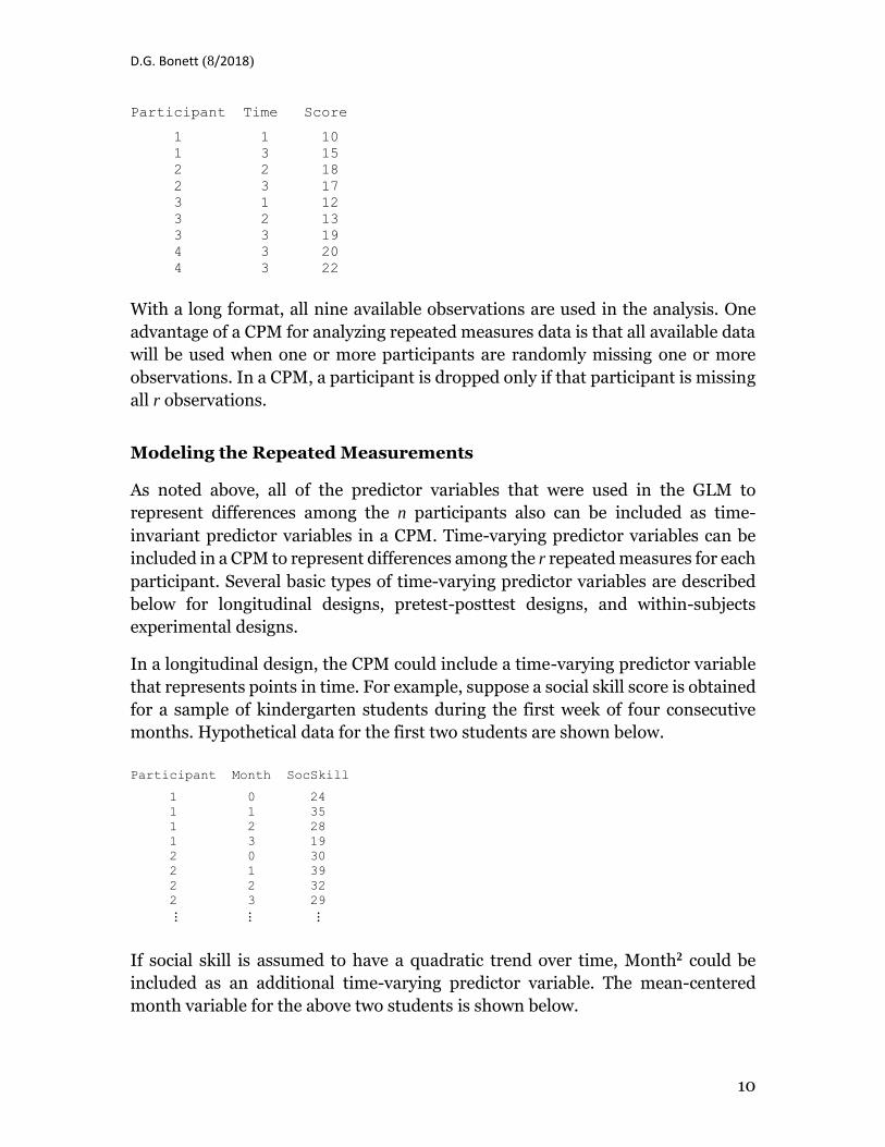
With a long format, all nine available observations are used in the analysis. One

advantage of a CPM for analyzing repeated measures data is that all available data

will be used when one or more participants are randomly missing one or more

observations. In a CPM, a participant is dropped only if that participant is missing

all r observations.

Modeling the Repeated Measurements

As noted above, all of the predictor variables that were used in the GLM to

represent differences among the n participants also can be included as time-

invariant predictor variables in a CPM. Time-varying predictor variables can be

included in a CPM to represent differences among the r repeated measures for each

participant. Several basic types of time-varying predictor variables are described

below for longitudinal designs, pretest-posttest designs, and within-subjects

experimental designs.

In a longitudinal design, the CPM could include a time-varying predictor variable

that represents points in time. For example, suppose a social skill score is obtained

for a sample of kindergarten students during the first week of four consecutive

months. Hypothetical data for the first two students are shown below.

Participant Month SocSkill

1 0 24

1 1 35

1 2 28

1 3 19

2 0 30

2 1 39

2 2 32

2 3 29

⋮ ⋮ ⋮

If social skill is assumed to have a quadratic trend over time, Month2 could be

included as an additional time-varying predictor variable. The mean-centered

month variable for the above two students is shown below.


11

Participant Month Month2 SocSkill

1 -1.5 2.25 24

1 -0.5 0.25 35

1 0.5 0.25 28

1 1.5 2.25 19

2 -1.5 2.25 30

2 -0.5 0.25 39

2 0.5 0.25 32

2 1.5 2.25 29

⋮ ⋮ ⋮ ⋮

A CPM model with only Month as a predictor variable implies a linear relation

between month and social skill as illustrated in Figure 3a. If Month2 is added to the

model, then the model implies a quadratic relation between month and social skill

as illustrated in Figure 3b.

In pretest-posttest designs, a dummy variable could be added to code treatment.

For example, suppose the social skill of each kindergarten student in the sample is

measured every month for two months before exposure to a social skill training

program and then every month for two months following training. Hypothetical

data for the first two students are shown below. Note that a dummy variable for

treatment is equal to 0 in months 1 and 2 and equal to 1 in months 3 and 4.

Participant Month Treatment SocSkill

1 0 0 24

1 1 0 35

1 2 1 28

1 3 1 24

2 0 0 30

2 1 0 39

2 2 1 32

2 3 1 30

⋮ ⋮ ⋮ ⋮

If a CPM for a longitudinal or pretest-posttest design only includes the Treatment

dummy variable as a predictor variable, the model implies a horizontal trend prior

to treatment and a jump after treatment that remains horizontal as illustrated in

Figure 3c. If both Month and the Treatment dummy variable are included as

predictor variables, the model implies a linear trend prior to treatment with a jump

following treatment with a linear trend following treatment that has the same slope

as during pretreatment time periods (see Figure 3d). If the pretreatment and

posttreatment slopes are expected to differ (see Figure 3e), then the product of

Month and Treatment can be added to the model as shown below.


12

Participant Month Treatment Month x Treatment SocSkill

1 0 0 0 24

1 1 0 0 35

1 2 0 0 28

1 3 1 3 24

1 4 1 4 35

2 0 0 0 30

2 1 0 0 39

2 2 0 0 32

2 3 1 3 30

2 4 1 4 39

⋮ ⋮ ⋮ ⋮ ⋮

In Figure 3e, there is a shift in the trend lines following treatment. If the

pretreatment slope is assumed to differ from the posttreatment slope but the two

lines are assumed to connect (see Figure 3f), this pattern can be modeled by

including only Month and Month x Treatment in the model.

(a) (b) (c)

Time Time Time

(d) (e) (f)

Time Time Time ________________________________________________

Figure 3. Examples of time trends

In within-subject experiments where participants are measured under all

treatment conditions in random or counterbalanced order, k – 1 dummy variables

are needed to represent the k-level treatment factor. For example, with k = 3

treatments, the data file would include two dummy variables as shown below with

hypothetical response variable scores for the first two participants.


13

Participant dummy1 dummy2 Score

1 1 0 61

1 0 1 57

1 0 0 78

2 1 0 54

2 0 1 62

2 0 0 48

⋮ ⋮ ⋮ ⋮

Time-varying covariates are random quantitative predictor variables that can be

included in longitudinal, pretest-posttest or within-subjects experimental designs.

For example, in the above within-subjects experiment, suppose the response

variable is the number of questions answered correctly after reading three short

reports. Participants vary in the length of time they read each report. If reading

time is related to reading comprehension, reading time could be included as a

time-varying covariate as illustrated below for the first two participants.

Participant dummy1 dummy2 Minutes Score

1 1 0 3.5 61

1 0 1 4.8 57

1 0 0 6.1 78

2 1 0 4.6 54

2 0 1 5.9 62

2 0 0 4.1 48

⋮ ⋮ ⋮ ⋮ ⋮

In longitudinal designs, lagged time-varying covariates are sometimes useful. A

one-period lagged covariate uses the value of the covariate at time t – 1 as the

predictor variable value at time t. For example, suppose a sample of first-year

college students agree to report their number of good friends and their loneliness

each month for six months. The researcher believes that the number of close

friends reported in the prior month is a predictor of loneliness in the current

month. Hypothetical friend and loneliness data are given below where the friend

variable has been lagged one month. With a one period lagged predictor variable,

the first time period (month = 0) is excluded from the analysis because the lagged

predictor variable value is usually unavailable at time 1.

Participant Month FriendsL1 Loneliness

1 1 2 46

1 2 3 44

1 3 2 44

1 4 4 38

1 5 6 30

2 1 3 37

2 2 3 35

2 3 4 30

2 4 4 28

2 5 5 20

⋮ ⋮ ⋮ ⋮


14

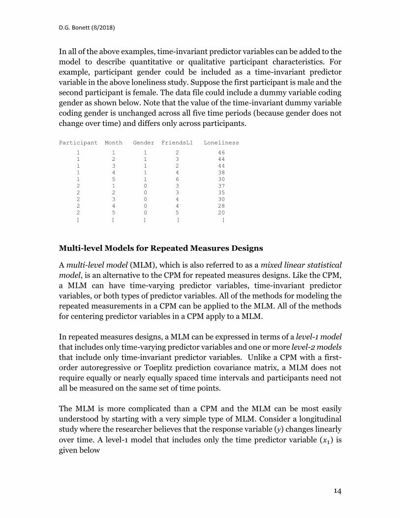
In all of the above examples, time-invariant predictor variables can be added to the

model to describe quantitative or qualitative participant characteristics. For

example, participant gender could be included as a time-invariant predictor

variable in the above loneliness study. Suppose the first participant is male and the

second participant is female. The data file could include a dummy variable coding

gender as shown below. Note that the value of the time-invariant dummy variable

coding gender is unchanged across all five time periods (because gender does not

change over time) and differs only across participants.

Participant Month Gender FriendsL1 Loneliness

1 1 1 2 46

1 2 1 3 44

1 3 1 2 44

1 4 1 4 38

1 5 1 6 30

2 1 0 3 37

2 2 0 3 35

2 3 0 4 30

2 4 0 4 28

2 5 0 5 20

⋮ ⋮ ⋮ ⋮ ⋮

Multi-level Models for Repeated Measures Designs

A multi-level model (MLM), which is also referred to as a mixed linear statistical

model, is an alternative to the CPM for repeated measures designs. Like the CPM,

a MLM can have time-varying predictor variables, time-invariant predictor

variables, or both types of predictor variables. All of the methods for modeling the

repeated measurements in a CPM can be applied to the MLM. All of the methods

for centering predictor variables in a CPM apply to a MLM.

In repeated measures designs, a MLM can be expressed in terms of a level-1 model

that includes only time-varying predictor variables and one or more level-2 models

that include only time-invariant predictor variables. Unlike a CPM with a first-

order autoregressive or Toeplitz prediction covariance matrix, a MLM does not

require equally or nearly equally spaced time intervals and participants need not

all be measured on the same set of time points.

The MLM is more complicated than a CPM and the MLM can be most easily

understood by starting with a very simple type of MLM. Consider a longitudinal

study where the researcher believes that the response variable (y) changes linearly

over time. A level-1 model that includes only the time predictor variable (𝑥1) is

given below


15

𝑦𝑖𝑗 = 𝑏0𝑖 + 𝑏1𝑖𝑥1𝑖𝑗 + 𝑒𝑖𝑗 (Model 5)

where the values of 𝑥1𝑖𝑗 are the time points at which participant i was measured.

For example, if participant 1 (i = 1) was measured on weeks 1, 2, 4, and 5 then 𝑥1𝑗1

would have values of 𝑥111 = 1, 𝑥112 = 2, 𝑥113 = 4, and 𝑥114 = 5; and if participant

2 (i = 2) was measured on weeks 1, 4, 6, 8, and 9 then 𝑥1𝑗2 would have values of

𝑥121 = 1, 𝑥122 = 4, 𝑥123 = 6, 𝑥124 = 8, and 𝑥125 = 9. Note that the time points need

not be equally spaced and different participants can be measured at different sets

of time points and different numbers of time points. Note also that the parameters

of the level-1 model contain an i subscript to indicate that each participant has their

own y-intercept (𝑏0𝑖) and slope (𝑏1𝑖) values. The prediction errors (𝑒𝑖𝑗) in the

level-1 model are typically assumed to be uncorrelated among participants and

have equal variances across participants and time (but this assumption can be

relaxed). Assuming equal variances, the variance of 𝑒𝑖𝑗 for all i and j is equal to 𝜎𝑒2.

The n participants are assumed to be a random sample from some specified study

population of N people. The level-1 model indicates that each of the N persons have

their own y-intercept and slope value. The level-1 model describes a random

sample of n participants and thus the 𝑏0𝑖 and 𝑏1𝑖 values (i = 1 to n) are a random

sample of a population of y-intercept and slope values. In the same way that a

statistical model describes a random sample of y scores, statistical models can be

used to describe a random sample of 𝑏0𝑖 and 𝑏1𝑖 values. The statistical models for

𝑏0𝑖 and 𝑏1𝑖 are called level-2 models.

The following level-2 models for 𝑏0𝑖 and 𝑏1𝑖 are the simplest type because they have

no predictor variables

𝑏0𝑖 = 𝛽0 + 𝑢0𝑖 (Model 6a)

𝑏1𝑖 = 𝛽1 + 𝑢1𝑖 (Model 6b)

where 𝑢0𝑖 and 𝑢1𝑖 are parameter prediction errors for the random values of 𝑏0𝑖

and 𝑏1𝑖, respectively. These parameter prediction errors can be correlated with

each other but they are assumed to be uncorrelated with the level-1 prediction

errors (𝑒𝑖𝑗). The n parameter prediction errors for 𝑏0𝑖 are assumed to be

uncorrelated with each other and have variances equal to 𝜎𝑢02 . Likewise, the n

parameter prediction errors for 𝑏1𝑖 are assumed to be uncorrelated with each other

and have variances equal to 𝜎𝑢12 . The value of 𝜎𝑢1

2 describes the variability of the 𝑏1𝑖

values in the population, and the value of 𝜎𝑢02 describes the variability of the 𝑏0𝑖


16

values in the population. The variability of the y-intercept values (𝑏0𝑖) is usually

interesting only if the variability of the slope values (𝑏1𝑖) is small. The graphs below

illustrate a sample of n = 5 participants where the slope variability is large (top)

and the slope variability is small (bottom).

Time

Time

In Model 6a, 𝛽0 is the population mean of the y-intercepts, and in Model 6b, 𝛽1 is

the population mean of the slope coefficients. MLM computer programs will

compute estimates of 𝛽0, 𝛽1, 𝜎𝑢02 , and 𝜎𝑢1

2 along with confidence intervals for 𝛽0, 𝛽1,

𝜎𝑢02 , and 𝜎𝑢1

2 . Confidence intervals for 𝜎𝑢0 and 𝜎𝑢1

, which are easier to interpret, are

obtained by taking the square roots of the confidence interval endpoints for 𝜎𝑢02

and 𝜎𝑢12 .

If the estimate of the slope variability (𝜎𝑢12 ) is small or uninteresting, this variance

can be constrained to equal 0 and then Model 6b reduces to 𝑏1𝑖 = 𝛽1. This level-2

model implies that the slope coefficient relating time to y is the same for everyone

in the population and equal to 𝛽1. If the confidence interval for 𝜎𝑢12 suggests that

𝜎𝑢12 is not small, this indicates that there is potentially interesting variability in the

slope coefficients among people in the study population. One or more predictor

variables can be included in Model 6b in an effort to explain some of the variability

in the slope coefficients.

In a MLM, the y-intercepts (𝑏0𝑖) are almost always assumed to be random. If the

confidence interval for 𝜎𝑢02 suggests that 𝜎𝑢0

2 is not small, this indicates that there

is potentially interesting variability in the y-intercepts among people in the study


17

population. One or more predictor variables can be included in Model 6a in an

effort to explain some of the variability in the y-intercepts.

The level-2 models can be substituted into the level-1 model to give the following

composite model

𝑦𝑖𝑗 = 𝛽0 + 𝛽1𝑥1𝑖𝑗 + 𝑒𝑖𝑗∗ (Model 7)

where 𝑒𝑖𝑗∗ = 𝑢0𝑖 + 𝑢1𝑖𝑥1𝑖𝑗 + 𝑒𝑖𝑗 is the composite prediction error for participant i at

time j. Although it was assumed that the level-1 prediction errors were

uncorrelated and homoscedastic, the composite prediction errors will be

correlated and could have unequal variances. Using covariance algebra (Appendix

of Module 2), the variance of 𝑒𝑖𝑗∗ at time j is

var(𝑒𝑖𝑗∗ ) = var(𝑢0) + 2𝑥1𝑗cov(𝑢0, 𝑢1) + 𝑥1𝑗

2 var(𝑢1) + var(e) (3.5)

and the covariance between two composite prediction errors at time 𝑗 and time 𝑗′

is

cov(𝑒𝑖𝑗

∗ , 𝑒𝑖𝑗′∗ ) = var(𝑢0) + (𝑥1𝑗 + 𝑥1𝑗′)cov(𝑢0, 𝑢1) (3.6)

The y-intercept (𝛽0) and the slope (𝛽1) in the composite model are identical to the

y-intercept (𝛽0) and slope (𝛽1) in a CPM that has only 𝑥1𝑖𝑗 as a time-varying

predictor variable. Unlike the CPM where the researcher can specify any type of

prediction error covariance structure (e.g., unstructured, Toeplitz, first-order

autoregressive), the MLM where the level-1 prediction errors are uncorrelated and

have equal variances has a composite prediction error covariance structure given

by Equations 3.5 and 3.6.

To illustrate the covariance structure implied by Equations 3.5 and 3.6, suppose

the estimates of var(𝑢0), var(𝑢1), cov(𝑢0, 𝑢1) and var(e), are 5.3, 2.4, -1.3, and 3.8,

respectively. Next, assume that the participants were measured on four equally

spaced time points with baseline centering so that 𝑥1𝑖1 = 0, 𝑥1𝑖2 = 1, 𝑥1𝑖3 = 2, and

𝑥1𝑖4 = 3. Plugging these values into Equations 3.5 and 3.6 gives the following 4 x 4

composite prediction error covariance matrix.

�̂� = [

9.14.02.71.4

4.0 8.9 1.40.1

2.7 1.4 1.4 0.1 13.5 − 1.2−1.2 22.9

]


18

With the assumption of a random y-intercept and a random slope, the resulting

composite prediction error covariance matrix assumes unequal variances that

decreases from 9.1 to 8.9 in periods 1 and 2 and then increases to 13.5 and 22.9 in

periods 3 and 4, respectively. Note also that the covariance between the measures

in periods 3 and 4 is assumed to be negative. This pattern of variances and

covariances could be very difficult to justify.

Treating the slope coefficient as random rather than fixed in a MLM can produce

a composite prediction error covariance structure that poorly approximates the

true composite prediction error covariance structure which in turn will give

misleading confidence interval and hypothesis testing results. The consequences

of treating a slope coefficient as random rather than fixed is most pronounced

when var(𝑢1) is large. One strategy is to reduce the value of var(𝑢1) by including

explanatory variables in the level-2 model. For example, suppose vocabulary size

is measured in a sample of preschool children each month for five consecutive

months. The slope coefficient for each child could vary considerable across

children (i.e., some children show large gains, some moderate gains, and others

very little gain) which would result in a large value of var(𝑢1). The researcher

suspects that younger children are more likely to have larger gains than older

children. The following level-2 models for Model 1 could then be specified.

𝑏0𝑖 = 𝛽0 + 𝛽02𝑥2𝑖 + 𝑢0𝑖 (Model 8a)

𝑏1𝑖 = 𝛽1 + 𝛽12𝑥2𝑖 + 𝑢1𝑖 (Model 8b)

where 𝑥2𝑖 is a time-invariant predictor variable that is equal to the age of child i at

the beginning of the study.

Any predictor variable that is used in the level-2 slope model is almost always used

in the level-2 y-intercept model because any variable that is related to the slope is

almost always related to the y-intercept. If age is a good predictor of the individual

slopes, then the var(𝑢1) could become much smaller compared to a level-2 model

that does not include age as a predictor variable.

Substituting Models 8a and 8b into the level-1 model (Model 7) gives the following

composite model

𝑦𝑖𝑗 = 𝛽0 + 𝛽1𝑥1𝑖𝑗 + 𝛽2𝑥2𝑖 + 𝛽12𝑥1𝑖𝑗𝑥2𝑖 + 𝑒𝑖𝑗∗ (Model 9)

where 𝑒𝑖𝑗∗ = 𝑢0𝑖 + 𝑢1𝑖𝑥1𝑖𝑗 + 𝑒𝑖𝑗. Note that the composite prediction error is the same

in Model 7. Note also that a level-2 predictor variable of a random slope coefficient

produces an interaction effect in the composite model. In this example, the


19

composite model includes an age x time interaction effect which describes a

relation between vocabulary size and time that depends on the child's age. The

parameters in Model 9 are identical to the parameters in a CPM (𝛽12 would be

labeled 𝛽3 in a CPM).

Suppose that when age is added to the level-2 models the estimates of var(𝑢0𝑖),

var(𝑢1), cov(𝑢0, 𝑢1) and var(e) are 3.5, 0.4, -0.05, and 1.7. Adding age in the level-2

models has reduced the estimate of var(𝑢1) from 2.4 to 0.4. The composite

prediction error covariance matrix with a baseline centered time variable is

�̂� = [

5.23.53.43.3

3.5 5.5 3.43.4

3.4 3.3 3.4 3.3 6.6 3.2 3.2 8.5

]

which now has similar variances and similar covariances. This covariance structure

assumes the variances increase over time from 5.2 to 8.5 which seems more

realistic than the previous example where the variances decreased and then

increased over time. This covariance structure, which also assumes that all

covariances are similar, would not be realistic in longitudinal and pretest-posttest

designs where the measurements obtained in adjacent time points are usually

more highly correlated than measurements separated by longer periods of time.

If the prediction errors in the level-1 model are assumed to be uncorrelated and

have equal variances, the composite prediction error covariance matrix in a MLM

will often be a poor approximation to the true composite prediction error

covariance matrix. To address this problem, MLM programs have options to

specify more realistic level-1 predictor error covariance structures. In longitudinal

and pretest-posttest designs, a first-order autoregressive prediction error structure

for the level-1 prediction errors usually gives a more realistic composite prediction

error covariance matrix. The level-1 prediction errors also could be assumed to

have unequal variances. Although MLM programs have options to specify more

general level-1 prediction error covariance structures, the parameter estimates of

these covariance structures are sometimes so highly correlated with the estimates

of 𝜎𝑢02 and 𝜎𝑢1

2 that the MLM program will not be able to provide unique estimates

of the covariance structure parameters and variances of the random y-intercepts

or random slopes. One strategy is to assume random y-intercepts and no random

slopes and then use the most general level-1 covariance structure that can be

estimated.


20

A Comparison Multi-level and Covariance Pattern Models

In a general MLM, the level-1 model can have multiple time-varying predictor

variables, and a level-2 model is specified for every parameter of the level-1 model.

Furthermore, each level-2 model can have no time-invariant predictor variables or

multiple time-invariant predictor variables. After the level-2 models are

substituted into the level-1 model, the resulting composite model will have the

same predictor variables as an equivalent CPM. Thus, MLM can estimate the same

parameters as a CPM. Unlike a CMP, a MLM also provides variance estimates of

the random coefficients. If the variance of any slope parameter in a MLM is large,

this suggest that the model is missing important interaction effects. Both the CPM

and the MLM can be implemented using "mixed linear model" programs in SAS,

SPSS, and R.

As noted previously, a CPM assumes every participant can be measured on the

same set of time points, and the first-order autoregressive and Toeplitz covariance

structures assume that the time points are equally or nearly equally spaced. In a

MLM, the time points can be unequally spaced and the time points need not be the

same for each participant.

The confidence interval and hypothesis testing methods in a CPM and MLM

require larger sample sizes in models where the prediction error covariance matrix

(in a CPM) or the composite prediction error covariance matrix (in a MLM) contain

many variance and covariance parameters to be estimated. In a MLM model with

only a random y-intercept, the composite prediction error covariance matrix has a

compound symmetric structure that requires the estimation of only two

parameters and this type of MLM can be applied in small samples even if the

number of repeated measurements is large. Of course, the compound symmetry

assumption could be unrealistic. Treating a slope coefficient as random will add

only two additional parameters (the variance of the random slope and the

covariance between the random y-intercept and the random slope) and could

produce a more realistic composite prediction error covariance matrix.

Alternatively, assuming a first-order autoregressive prediction error covariance

structure in the level-1 model could produce a more realistic composite prediction

error covariance structure.

If the covariance structure of the composite prediction errors in a MLM are a poor

approximation to the correct covariance structure, then the hypothesis testing and

confidence interval results for the parameters of the composite model could be

misleading.


21

The Akaike Information Criterion (AIC) can be used to assess the effects of

treating one or more random slope coefficients as random rather than fixed. The

AIC also can be used to assess the effect of using different level-1 prediction error

covariance structures in a MLM or different prediction error covariance structures

in a CPM. When comparing two models with the same predictor variables, the

model with the smaller AIC value suggests a more appropriate composite

prediction error structure. For example, if the AIC in a CPM for a first-order

autoregressive structure (with require the estimation of only two parameters) is

smaller than the AIC for an unstructured prediction error matrix, this could justify

the use of the first-order autoregressive covariance structure. If the true prediction

error covariance structure can be closely approximated by a simple covariance

structure, then the hypothesis testing and confidence interval results in a CPM

should perform better in small samples than a CPM that uses an unstructured

prediction error covariance matrix.

In repeated measures designs where a CPM and a MLM are both appropriate, one

recommendation is to use both models. First, the parameters of the CMP are

estimated using the most realistic prediction covariance matrix, such as an

unstructured, heteroscedastic Toeplitz, or heteroscedastic compound symmetric

prediction error covariance matrix. Next, a MLM could be used to obtain estimates

and confidence intervals for the variances of the random y-intercept and any

random slope coefficients. If the variance of any random slope coefficient is large,

this suggests the need for additional predictor variables in the level-2 models

which implies a need for additional interaction effects in the CPM.

Random Factors

All of the factors considered in Module 2 of PSYC 204 and Module 2 of this course

have been fixed factors because it was assumed that the factor levels used in the

study were deliberately selected and were the only factor levels of interest. In

comparison, the levels of a random factor are randomly selected from a large

superpopulation of M possible factor levels. The appeal of using a random factor

is that the statistical results apply to all M levels of the random factor even though

only a small subset of the factor levels are actually used in the study. With a fixed

factor, the statistical results apply only to the factor levels included in the study.

Recall that a factor can be a classification factor or a treatment factor. With a

classification factor, participants are classified into the levels of the factor based on

some existing characteristic of the participant. The levels of a classification factor

define different subpopulations of people. With a treatment factor, participants are

randomly assigned to the levels of the factor. A random factor can be a random


22

classification factor or a random treatment factor. Most random factors are

classification factors and only random classification factors will be illustrated here.

In studies where a large number (M) of subpopulations could be examined, such

as all schools in a state, all neighborhoods in a large city, or all branch offices of a

large organization, it could be costly or impractical to take a random sample of

participants from each of the M subpopulations. In these situations, the researcher

could randomly select k subpopulations from the superpopulation of M

subpopulations (e.g., schools, neighborhoods, branch offices) and then take a

random sample of 𝑛𝑗 participants from each of the k subpopulations. This type of

sampling is called two-stage cluster sampling.

A linear statistical model with one random factor and no other factors or covariates

is called a one-way random effects ANOVA model and the population means of

interest are 𝜇1, 𝜇2, … , 𝜇𝑀. Although only k of these M population means will be

estimated in the study, it is possible to obtain a confidence interval for the

superpopulation mean 𝜇 = (𝜇1 + 𝜇2 + … + 𝜇𝑀)/𝑀. With equal sample sizes per

group (and equal to n), a 100(1 − 𝛼)% confidence interval for 𝜇 is

�̂� ± 𝑡𝛼/2;(𝑘−1)√𝑀𝑆𝐴/𝑘𝑛 (3.7)

where �̂� = (�̂�1 + �̂�2 + … + �̂�𝑘)/𝑘 and MSA is the mean square estimate for the

between-subjects factor in a one-way ANOVA (see Module 2 of PSYC 204).

The standard deviation of the M population means is 𝜎𝜇 =√∑ (𝜇𝑗 − 𝜇)2𝑀𝑗=1 /𝑀 , which

is a measure of effect size because larger values of 𝜎𝜇 represent larger differences

among the population means. A standardized measure of effect size in designs with

a random factor is 𝜂2 = 𝜎𝜇2/(𝜎𝜇

2 + 𝜎𝑒2), where 𝜎𝑒

2 is the within-group error variance.

An estimate of 𝜎𝜇2 is

�̂�𝜇2 = (𝑀𝑆A – 𝑀𝑆E)/𝑛, (3.8)

an estimate of 𝜂2 is

�̂�2 = (𝑀𝑆A – 𝑀𝑆E)/[𝑀𝑆A + (𝑛 − 1)𝑀𝑆E], (3.9)

and an estimate of 𝜎𝑒2 is MSE where MSA and MSE are the mean square estimates

from a one-way ANOVA table. Recall from PSYC 204 that a confidence interval for

𝜂2 in the one-way ANOVA involved complicated computations. Surprisingly, a


23

confidence interval for 𝜂2 in the one-way random effects ANOVA can be hand

computed. The 100(1 − 𝛼)% lower (L) and upper (U) confidence limits for 𝜂2 are

L = (F/𝐹𝛼/2; 𝑑𝑓1,𝑑𝑓2 – 1)/( 𝑛 + F/𝐹𝛼/2; 𝑑𝑓1,𝑑𝑓2 – 1) (3.10a)

U = (F/𝐹1−𝛼/2; 𝑑𝑓1,𝑑𝑓2 – 1)/(𝑛 + F/𝐹1−𝛼/2; 𝑑𝑓1,𝑑𝑓2 – 1) (3.10b)

where F = MSA/MSE, 𝐹𝛼/2; 𝑑𝑓1,𝑑𝑓2 and 𝐹1−𝛼/2; 𝑑𝑓1,𝑑𝑓2 are critical F values with df1 =

k – 1 and df2 = k(n – 1). The qf function in R can be used to obtain these critical F

values.

The one-way random effect ANOVA can be expressed as special type of MLM. The

level-1 model can be expressed as

𝑦𝑖𝑗 = 𝜇𝑗 + 𝑒𝑖𝑗 (3.11)

where 𝜇𝑗 is the subpopulation mean for level j of the random factor. With randomly

selected factor levels, the 𝜇𝑗 values (j = 1 to k) are a random sample from the

superpopulation of 𝜇𝑗 values. A level-2 model for the random 𝜇𝑗 values is

𝜇𝑗 = 𝜇 + 𝑢𝑗 (3.12)

where 𝜇 is defined above and 𝑢𝑗 is a parameter prediction error that is assumed to

be uncorrelated with 𝑒𝑖𝑗. The variance of 𝜇𝑗 is 𝜎𝜇2 which also was defined above.

Substituting the level-2 model into the level-1 model gives the following composite

model

𝑦𝑖𝑗 = 𝜇 + 𝑒𝑖𝑗∗ (3.13)

where 𝑒𝑖𝑗∗ = 𝑒𝑖𝑗 + 𝜇𝑗. Using covariance algebra, the variance of 𝑒𝑖𝑗

∗ (for every value

of i and j) is equal to 𝜎𝜇2 + 𝜎𝑒

2, and the covariance between any two participants

within the same factor level is equal to 𝜎𝜇2. Thus, the correlation between two

participants within the same factor level is equal to 𝜎𝜇2/(𝜎𝜇

2 + 𝜎𝑒2), which was

defined above as 𝜂2 but is also called an intraclass correlation because it describes

the correlation between any two participant scores within the same factor level.

Mixed linear model programs can be used to obtain hypothesis tests and

confidence intervals for 𝜇 and 𝜎𝜇2.

One or more person-level predictor variables can be added to Equation 3.11. The

predictor variables can be indicator variables or quantitative variables. When all of


24

the predictor variables are quantitative, the resulting composite model is referred

to as a one-way random effect ANCOVA model. One or more group-level predictor

variables, which can be indicator variables or quantitative variables, can be added

to Equation 3.12 to explain some of the variability in the group means. Mixed linear

model programs are required to obtain hypothesis tests and confidence intervals

in these more general random factor models.

Assumptions

Hypothesis tests and confidence interval for the parameters of a CPM assume the

n participants have been randomly sampled from some population (the random

sampling assumption) and the responses from one participant are uncorrelated

with the responses of any other participant (the independence assumption). The r

responses from any single participant are not required to be uncorrelated, but any

structured prediction error covariance matrix in a CPM (e.g., compound

symmetric, first-order autoregressive, Toeplitz) specified by the researcher must

closely approximate the true variances and covariances among the r responses. The

first-order autoregressive and Toeplitz covariance structures that could be used in

a CPM assume equally or nearly equally spaced time points in longitudinal and

pretest-posttest designs. If the sample size is large enough, specifying an

unstructured prediction error covariance matrix is usually recommended. The

prediction errors are assumed to have an approximate normal distribution in the

population (the prediction error normality assumption). The prediction error

normality assumption is usually not a concern if the number of participants (n) is

greater than about 20.

The random sampling assumption, the independence assumption, and the

prediction error normality assumption are also required in a MLM. The composite

prediction error normality assumption is usually not a concern if the number of

participants (n) is greater than about 20. The variances of the random coefficients

are additional parameters in a MLM. Hypothesis tests and confidence intervals for

the random coefficient variances assume that the coefficient values in the

population have an approximate normal distribution (the random coefficient

normality assumption). Hypothesis tests and confidence intervals for the random

coefficient variances are very sensitive to minor violations of the random

coefficient normality assumption and increasing the sample size will not mitigate

the problem. Specifically, a confidence interval for a random coefficient variance

can have a true coverage probability that is far less than 1 – 𝛼 if the distribution of

person level coefficient values in the population are leptokurtic, regardless of

sample size. The widths of the confidence intervals for the variances of the random

parameters depend primarily on the sample size (n) rather than r. A large sample


25

size is usually needed to obtain a usefully narrow confidence interval for a random

coefficient variance. One of the advantages of the MLM over the CPM is the ability

to assess the variability of the random intercept and slopes but this advantage is

diminished given the random coefficient normality assumption of the MLM.

The assumptions for a random effects ANOVA model include all the assumptions

for the fixed-x GLM described in Module 2 in addition to several other important

assumptions. The consequences of violating the GLM assumptions also hold in the

random effects ANOVA model. In addition to the GLM assumptions, the random

effects ANOVA model assumes that the factor levels have been randomly selected

from a definable superpopulation of factor levels. If this assumption cannot be

justified, then the confidence interval for the superpopulation mean (Equation 3.7)

will be uninterpretable. The random effects ANOVA model also assumes that the

superpopulation distribution of means has an approximate normal distribution.

Violating this assumption is usually not a problem for Equation 3.7 if k (the number

of factor levels) greater than about 30. However, the confidence interval for 𝜂2 can

have a true coverage probability that is far less than 1 – 𝛼 if the superpopulation

means are leptokurtic regardless of sample size. The parameter prediction errors

(𝑢𝑗) are assumed to be uncorrelated with the person-level prediction errors (𝑒𝑖𝑗).

Violating this assumption will introduce bias into the estimate of 𝜂2 regardless of

sample size.

In repeated measures studies where either a CPM or a MLM could be used, a CPM

with the least restrictive prediction error covariance matrix (e.g., heteroscedastic

Toeplitz or unstructured) should be used to estimate the composite model

parameters. If the sample size is sufficiently large and the random coefficient

normality assumption is plausible, a MLM could be used next to obtain confidence

intervals for the variances of the random coefficients. A large variance for any

random slope indicates the omission of important interaction effects and the need

for additional research to discover these interaction effects. When designing a

longitudinal or pretest-posttest, the researcher should plan to measure each

participant on the same set of equally or nearly equally spaced time points, so that

a CPM can be used, and obtain a sample size that is large enough to use an

unrestricted prediction error covariance matrix in the CMP. Using the smallest

number of time points needed to assess the effects of the time-varying predictor

variables will improve the small-sample performance of the confidence interval

and hypothesis tests when using an unrestricted prediction error covariance

structure.