


Languages
Pages
Legal


Modeling Volatility of S&P 500 Index Daily Returns:
A comparison between model based forecasts and implied volatility
Huang Kun
Department of Finance and Statistics
Hanken School of Economics
Vasa
2011
HANKEN SCHOOL OF ECONOMICS
Department of: Finance and Statistics Type of work: Thesis
Author: Huang Kun Date: April, 2011
Title of thesis:
Modeling Volatility of S&P 500 Index Daily Returns: A comparison between model
based forecasts and implied volatility
Abstract:
The objective of this study is to investigate the predictability of model based
forecasts and the VIX index on forecasting future volatility of S&P 500 index daily
returns. The study period is from January 1990 to December 2010, including 5291
observations.
A variety of time series models were estimated, including random walk model,
GARCH (1,1), GJR(1,1) and EGARCH (1,1) models. The study results indicate that GJR
(1,1) outperforms other time series models for out-of-sample forecasting. The forecast
performance of VIX, GJR(1,1) and RiskMetrics were compared using various
approaches. The empirical evidence does not support the view that implied volatility
subsumes all information content, and the study results provide strong evidence
indicating that GJR (1,1) outperforms VIX and RiskMetrics for modeling future
volatility of S&P 500 index daily returns.
Additionally, the results of the encompassing regression for future realized
volatility at 5-, 10-, 15-, 30- and 60-day horizons, and the results of the encompassing
regression for squared return shocks suggest that the joint use of GJR (1,1) and
RiskMetrics can produce the best forecasts.
By and large, our finding indicates that implied volatility is inferior for future
volatility forecasting, and the model based forecasts have more explanatory power for
future volatility.
Keywords: volatility, S&P 500, GARCH, GJR, RiskMetrics, implied volatility

CONTENTS
1 Introduction………………………………………………………………………………………………………2
2 Literature Review……………………………………………………………………………………………….6
3 The CBOE Volatility Index – VIX………………………………………………………………………16
3.1 Implied Volatility……………………………………………………………………………………….16
3.2 The VIX Index……………………………………………………………………………………………17
4 Time Series Models for Volatility Forecasting…………………………………………………… 19
4.1 Random Walk Model………………………………………………………………………………….19
4.2 The ARCH(q) Model……………………………………………………………………….………… 19
4.3 The GARCH (p,q) Model………………………………………………………………….…………20
4.3.2 The Stylized Facts of Volatility……………………………………………….…………21
4.4 The GJR (p,q) Model…………………………………………………………………………………23
4.5 The EGARCH (p,q) Model…………………………………………………………………………..24
4.6 RiskMetrics Approach…………………………………………………………………………………25
5 Practical Issues for Model-building……………………………………………………………………26
5.1 Test ARCH Effect………………………………………………………………………………………26
5.2 Information Criterion…………………………………………………………………………………27
5.3 Evaluating the Volatility Forecasts……………………………………………………………….27
5.3.1 Out-of-sample Forecast………………………………………………………………………..27
5.3.2 Traditional Evaluation Statistics…………………………………………………………..28
6 Data………………………………………………………………………………………………………………30
6.1 S&P 500 Index Daily Returns………………………………………………………………………30
6.1.1 Autocorrelation of S&P 500 Index Daily Returns……………………………………32
6.1.2 Testing ARCH Effect of S&P 500 Index Daily Returns……………………………33
6.2 Properties of the VIX Index…………………………………………………………………………34
6.3 Study on S&P 500 Index and the VIX Index………………………………………………….34
6.3.1 Cross-correlation between S&P 500 Index and the VIX Index……………….34

6.3.2 S&P 500 Index Daily Returns and the VIX Index………………………………..37
7 Estimation and Discussion……………………………………………………………………………….43
7.1 Model Selection…………………………………………………………………………………………43
7.2 Test Numerical Accuracy of GARCH Estimates……………………………………………45
7.3 Estimates of Models…………………………………………………………………………………..46
7.4 BDS Test…………………………………………………………………………………………………...49
7.5 Graphical Diagnostic………………………………………………………………………………….51
8 Forecast Performance of Model Based Forecasts and VIX…………………………………..53
8.1 Out-of-sample Forecast Performance of GARCH Models……………………………..53
8.2 In-sample Forecast Performance of VIX……………………………………………………..54
8.3 Comparing Predictability of Time Series Models and VIX…………………………….56
8.3.1 Correlation between Realized Volatility and Volatility Forecasts…………59
8.3.2 Regression for In-sample Realized Volatility……………………………………..60
8.3.3 Residual Tests for Regression of In-sample Realized Volatility……………64
8.3.4 Regression for Out-of-sample Realized Volatility………………………………67
8.3.5 Residual Tests for Regression of Out-of-sample Realized Volatility…….70
8.3.6 Encompassing Regression for Realized Volatility………………………………72
8.3.7 Average Squared Deviation……………………………………………………………..75
8.3.8 Regression for Squared Return Shocks……………………………………………76
8.3.9 Encompassing Regression for Squared Daily Return Shocks……………..78
9 Conclusion…………………………………………………………………………………………………….80
References………………………………………………………………………………………………………….81
Appendix A. VIX and Future Realized Volatility…………………………………………………….86
Appendix B. Out-of-sample Forecast Performance on Realized Volatility………………..89
Appendix C. Residuals from Regression for Out-of-sample Realized Volatility…………91
TABLES
Table 1.Summary statistics for S&P 500 index daily returns 31
Table 2 Test for ARCH effect in S&P 500 daily index returns 33
Table 3. Summary statistics of the VIX index 34
Table 4. Cross-correlation between S&P 500 index daily returns and
implied volatility index 35
Table 5. Regression results for VIX changes and S&P 500 index daily returns 38
Table 6. Information criteria for estimated GARCH (p,q) models 44
Table 7. The summary statistics of estimated volatility models 47
Table 8. BDS test for serial independence in residuals 50
Table 9. Forecast Performance of GARCH models 53
Table 10. In-sample forecast performance of VIX and GARCH specifications 55
Table 11 Correlation between Realized Volatility and Alternative Forecasters 59
Table 12. Performance of regression for in-sample realized volatility 61
Table 13. Forecast performance on out-of-sample realized volatility 63
Table 14. Residual tests for regression for in-sample realized volatility 66
Table 15. Performance of regression for out-of-sample realized volatility 68
Table 16. Residual tests for regression for out-of-sample realized volatility 71
Table 17. Encompassing regression for realized volatility 74
Table 18. The average squared deviation from alternative approaches 76
Table 19. Regression results for squared return shocks 77
Table 20. Encompassing regression results for squared return shocks 78
FIGURES
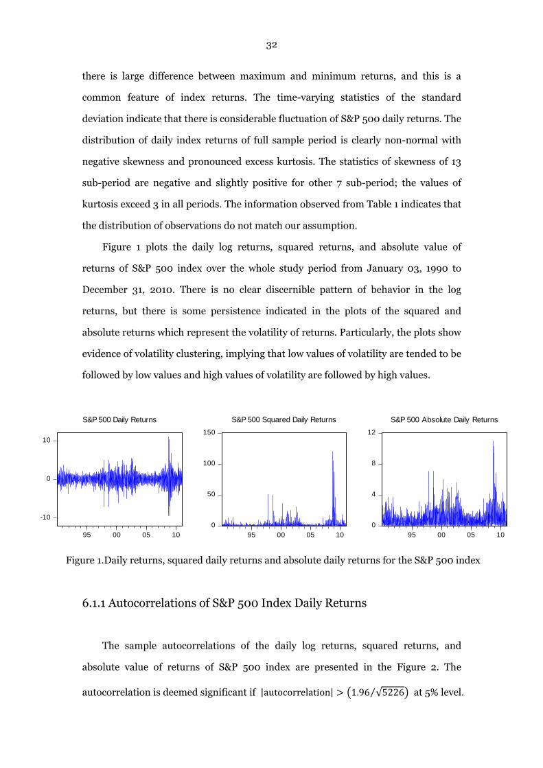
Figure 1.Daily returns, squared daily returns and absolute daily returns
for the S&P 500 index 32
Figure 2. Autocorrelation of , and | | for S&P 500 index 33
Figure 3. S&P 500 Index (logarithm) and the VIX Index 36
Figure 4. S&P 500 index daily returns and the VIX index 41
Figure 5 S&P 500 index absolute daily returns and the VIX index 42
Figure 6. Estimates from various GARCH (p,q) models 45
Figure 7. Graphical residual diagnostics from GARCH (1,1) to S&P 500 returns 52
2
1 Introduction
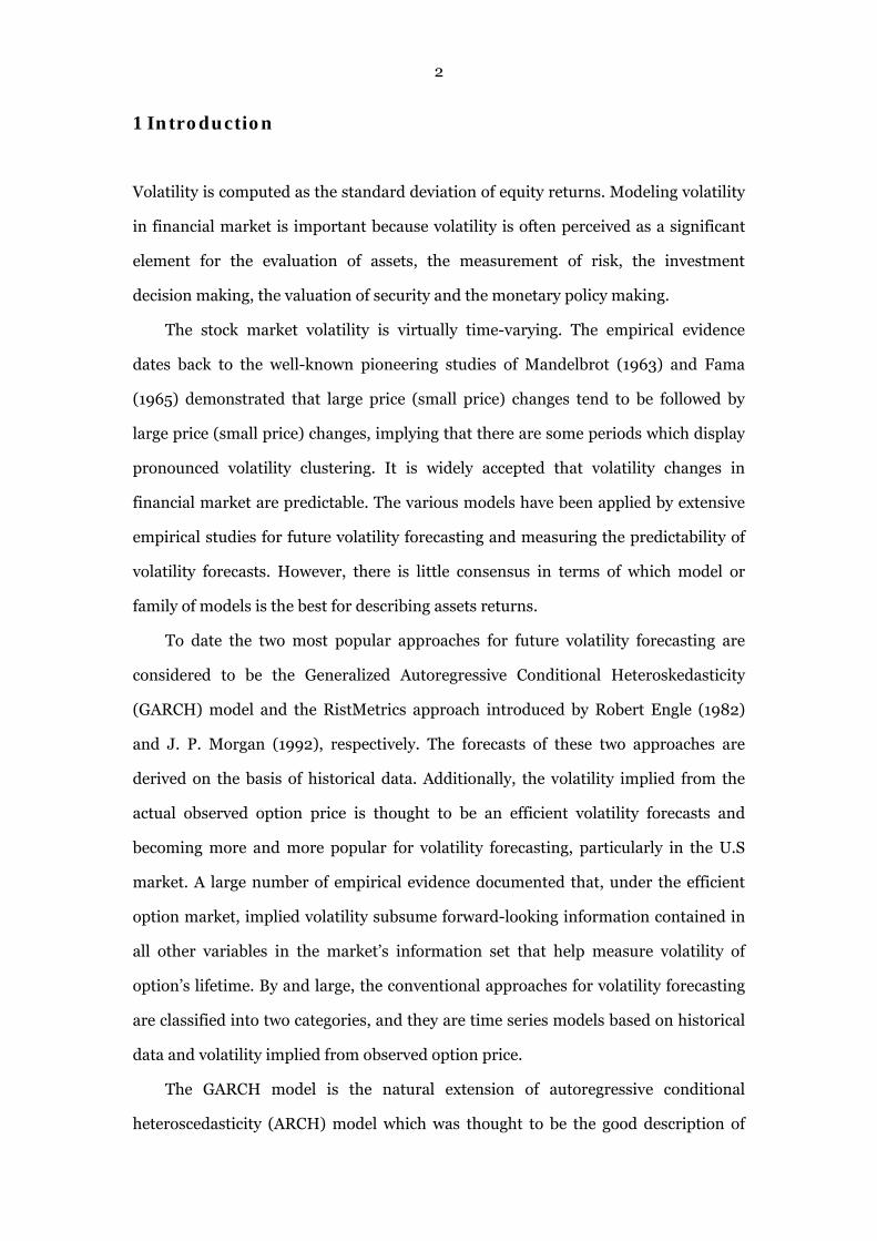
Volatility is computed as the standard deviation of equity returns. Modeling volatility
in financial market is important because volatility is often perceived as a significant
element for the evaluation of assets, the measurement of risk, the investment
decision making, the valuation of security and the monetary policy making.
The stock market volatility is virtually time-varying. The empirical evidence
dates back to the well-known pioneering studies of Mandelbrot (1963) and Fama
(1965) demonstrated that large price (small price) changes tend to be followed by
large price (small price) changes, implying that there are some periods which display
pronounced volatility clustering. It is widely accepted that volatility changes in
financial market are predictable. The various models have been applied by extensive
empirical studies for future volatility forecasting and measuring the predictability of
volatility forecasts. However, there is little consensus in terms of which model or
family of models is the best for describing assets returns.
To date the two most popular approaches for future volatility forecasting are
considered to be the Generalized Autoregressive Conditional Heteroskedasticity
(GARCH) model and the RistMetrics approach introduced by Robert Engle (1982)
and J. P. Morgan (1992), respectively. The forecasts of these two approaches are
derived on the basis of historical data. Additionally, the volatility implied from the
actual observed option price is thought to be an efficient volatility forecasts and
becoming more and more popular for volatility forecasting, particularly in the U.S
market. A large number of empirical evidence documented that, under the efficient
option market, implied volatility subsume forward-looking information contained in
all other variables in the market’s information set that help measure volatility of
option’s lifetime. By and large, the conventional approaches for volatility forecasting
are classified into two categories, and they are time series models based on historical
data and volatility implied from observed option price.
The GARCH model is the natural extension of autoregressive conditional
heteroscedasticity (ARCH) model which was thought to be the good description of

3
stock returns and an efficient technique for estimating and analyzing time-varying
volatility in stock returns. The seminal ARCH (q) model was pioneered by Engle
(1982), representing a function of the squared returns of the past q periods and
formulating the conditional variance of returns via maximum likelihood procedure
rather than making use of the sample standard deviation. However, there are some
limitations of ARCH (q) model. For example, how to decide the appropriate number
of lags of the squared residual in the model; the large value of q may induce a non-
parsimonious conditional variance model; non-negative constraints might be
violated.
Some problems of ARCH (q) model can be overcome by GARCH (p,q) model
which incorporates the additional dependencies on p lags of the past volatility and
the variance of residuals is modeled by an autoregressive moving average ARMA (p,q)
process replacing the AR (q) process of ARCH (q) model. GARCH (p,q) model is
widely used in practice. The extensive empirical evidence suggest that GARCH (p,q)
model is a more parsimonious model than ARCH (q) model and provides a
framework for deeper time-varying volatility estimation. One of outstanding features
of the GARCH (p,q) model is that it can effectively remove the excess kurtosis in
returns. Particularly, GARCH (1,1) model is widely recognized as the most popular
framework for modeling volatilities of many financial time series.
However, the standard symmetric GARCH (p,q) model also has some
underlying limitations. For instance, the requirement that the conditional variance is
positive may be violated for the estimated model. The only way to avoid this problem
is to place the constraints for coefficients to force them to be positive. The second
limitation is that it cannot explain the leverage effect, although it has good
performance for explaining volatility clustering and leptokurtosis in a time series.
Thirdly, the direct feedback between the conditional mean and conditional variance
is not allowed by the standard GARCH (p,q) model.
In order to overcome the limitations of the standard symmetric GARCH (p,q)
model, a number of extensions have been introduced, such as the asymmetric GJR
(p,q) and EGARCH (p,q) models which can better capture the dynamics of time series

4
and make the modeling more flexible.
As another conventional approach for volatility forecasting, implied volatility is
the volatility implied from observed option price and computed by option pricing
formulas, such as the Black-Scholes formula which is widely used in practice. As we
know, the required parameters for computing option price using Black-Scholes model
are stock price, strike price, risk free interest rate, time to maturity, volatility as well
as dividend. Being the unique unknown parameter, implied volatility is thought to be
the representation of the future volatility by consensus because option is priced on
the basis of future payoffs.
Today, implied volatility indices have been constructed and published by stock
exchange in many countries, and it is widely recognized that implied volatility index
has superior predictability for future stock market volatility. A common question
regarding to implied volatility is whether the option price subsumes all relevant
information about future volatility. The large number of empirical evidence from
previous studies (e.g., Fleming, Ostdiek and Whaley 1995, Christensen and Prabhala
1998, Giot 2005a, Giot 2005b, Corrado and Miller, JR. 2005, Giot and Laurent 2006,
Frijns, Tallau and Tourani-Rad 2008, Becker, Clements and McClelland 2009,
Becker, Clements and Coleman-Fenn 2009, Frijns, Tallau and Tourani-Rad 2010)
demonstrate that implied volatility is a forward-looking measure of market volatility.
However, the poor predictive power of implied volatility was also indicated by some
studies, such as Day and Lewis (1992), Canina and Figlewski (1993), Becker,
Clements and White (2006), Becker, Clements and White (2007) and Becker and
Clements (2008).
The objective of our study is to investigate whether the model based forecasts or
the CBOE volatility index (the VIX index published by Chicago Board Options
Exchange) is superior on forecasting future volatility of S&P 500 index daily returns
The data used for our study ranges from January 1990 to December 2010. There are
several reasons why we consider the use of the VIX index. First, it is on the basis of
S&P 500 index which is considered to be the core index for the U.S equity market.
Second, VIX is widely believed as the market’s expectation of S&P 500 index. Third,
5
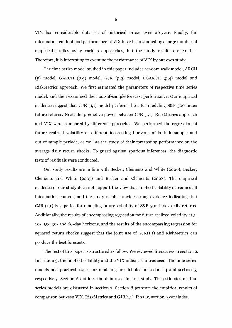
VIX has considerable data set of historical prices over 20-year. Finally, the
information content and performance of VIX have been studied by a large number of
empirical studies using various approaches, but the study results are conflict.
Therefore, it is interesting to examine the performance of VIX by our own study.
The time series model studied in this paper includes random walk model, ARCH
(p) model, GARCH (p,q) model, GJR (p,q) model, EGARCH (p,q) model and
RiskMetrics approach. We first estimated the parameters of respective time series
model, and then examined their out-of-sample forecast performance. Our empirical
evidence suggest that GJR (1,1) model performs best for modeling S&P 500 index
future returns. Next, the predictive power between GJR (1,1), RiskMetrics approach
and VIX were compared by different approaches. We performed the regression of
future realized volatility at different forecasting horizons of both in-sample and
out-of-sample periods, as well as the study of their forecasting performance on the
average daily return shocks. To guard against spurious inferences, the diagnostic
tests of residuals were conducted.
Our study results are in line with Becker, Clements and White (2006), Becker,
Clements and White (2007) and Becker and Clements (2008). The empirical
evidence of our study does not support the view that implied volatility subsumes all
information content, and the study results provide strong evidence indicating that
GJR (1,1) is superior for modeling future volatility of S&P 500 index daily returns.
Additionally, the results of encompassing regression for future realized volatility at 5-,
10-, 15-, 30- and 60-day horizons, and the results of the encompassing regression for
squared return shocks suggest that the joint use of GJR(1,1) and RiskMetrics can
produce the best forecasts.
The rest of this paper is structured as follow. We reviewed literatures in section 2.
In section 3, the implied volatility and the VIX index are introduced. The time series
models and practical issues for modeling are detailed in section 4 and section 5,
respectively. Section 6 outlines the data used for our study. The estimates of time
series models are discussed in section 7. Section 8 presents the empirical results of
comparison between VIX, RiskMetrics and GJR(1,1). Finally, section 9 concludes.
6
2 Literature Review
The predictability of ARCH (q) model on volatility of equity returns has been studied
by extensive literature. However, the empirical evidence indicating the good forcast
performance of ARCH (q) model are sporadic. The previous studies by Franses and
Van Dijk (1996), Braisford and Faff (1996) and Figlewski (1997) examined the
out-of-sample forecast performance of ARCH (q) models, and their study results are
conflict. However, the common ground of their studies is that the regression of
realized volatility produce a quite low statistic of R2. Since the average R2 is smaller
than 0.1, they suggested that ARCH (q) model has weak predictive power on future
volatility.
There is a variety of restrictions influencing the forecasting performance of
ARCH models. The frequency of data is one of restrictions, and it is an issue widely
discussed in preceding papers. Nelson (1992) studied ARCH model and documented
that the ARCH model using high frequency data performs well for volatility
forecasting, even when the model is severely misspecified. However, the
out-of-sample forecasting ability of medium- and long-term volatility is poor.
The existing literature regarding to the study on GARCH type models can be
classified into two categories, and they are the investigation on the basic symmetric
GARCH models and the GARCH models with various volatility specifications.
Wilhelmsson (2006) investigated the forecast performance of the basic GARCH
(1,1) model by estimating S&P 500 index future returns with nine different error
distributions, and found that allowing for a leptokurtic error distribution leads to
significant improvements in variance forecasts compared to using the normal
distribution. Additionally, the study also found that allowing for skewness and time
variation in the higher moments of the distribution does not further improve
forecasts.
Chuang, Lu and Lee (2007) studied the volatility forecasting performance of the
standard GARCH models based on a group of distributional assumptions in the
context of stock market indices and exchange rate returns. They found that the

7
GARCH model combined with the logistic distribution, the scaled student’s t
distribution and the Riskmetrics model are preferable both stock markets and foreign
exchange markets. However, the complex distribution does not always outperform a
simpler one.
Franses and van Dijk (1996) examined the predictability of the standard
symmetric GARCH model as well as the asymmetric Quadratic GARCH and GJR
models on weekly stock market volatility forecasting, and the study results indicated
that the QGARCH model has the best forecasting ability on stock returns within the
sample period.
Brailsford and Faff (1996) investigated the predictive power of various models on
volatility of the Australia stock market. They tested the random walk model, the
historical mean model, the moving average model, the exponential smoothing model,
the exponential weighted moving average model, the simple regression model, the
symmetric GARCH models and two asymmetric GJR models. The empirical evidence
suggested that GJR model is the best for forecasting the volatility of Australia stock
market returns.
Chong, Ahmad and Abdullah (1999) compared the stationary GARCH,
unconstrained GARCH, non-negative GARCH, GARCH-M, exponential GARCH and
integrated GARCH models, and they found that exponential GARCH (EGARCH)
performs best in describing the often-observed skewness in stock market indices and
in out-of-sample (one-step-ahead) forecasting.
Awartani and Corradi (2005) studied the predictability of different GARCH
models, particularly focused on the predictive content of the asymmetric component.
The study results show that GARCH models allowing for asymmetries in volatility
produce more accurate volatility predictions.
Evans and McMillan (2007) studied the forecasting performance of nine
competing models for daily volatility for stock market returns of 33 economies. The
empirical results show that GARCH models allowing for asymmetries and
long-memory dynamics provide the best forecast performance.

8
By and large, the extensive empirical studies and evidence demonstrated that
GARCH models allowing for asymmetries perform very well for modeling future
volatility.
EWMA model is also a widely used technique for modeling and forecasting
volatility of equity returns in financial markets, and the well-known RiskMetrics
approach is virtually the variation of EWMA. A great deal of existing studies using
EWMA model on various markets demonstrated that EWMA model has different
performance.
Akgiray (1989) first examined the forecast performance of EWMA technique on
volatility forecasting for stocks on the NYSE. The study also examined predictability
of ARCH and GARCH models. The finding indicated that EWMA model is useful for
forecasting time series, however, the GARCH model performs best for forecasting
volatility.
Tse (1991) studied volatility of stock returns of Japanese market during the
period of 1986 to 1989 using ARCH, GARCH and EWMA models. The study results
revealed that the EWMA model outperforms ARCH and GARCH models for volatility
forecasting of stock returns in Tokyo Stock Exchange during the sample period.
Tse and Tung (1992) investigated monthly volatility movements in Singapore
stock market using three different volatility forecasting models which are the naive
method based on historical sample variance, EWMA and GARCH models. The study
results suggested that EWMA model is the best for predicting volatility of monthly
returns for Singapore market.
Wash and Tsou (1998) investigated the volatility of Australian index from
January 1, 1993 to December 31, 1995 using a variety of forecasting techniques, and
they are historical volatility, an improved extreme-value method, the ARCH/GARCH
class of models, and EWMA model. The hourly data, daily data and weekly data were
used, respectively. The finding indicated that the EWMA model outperforms other
volatility forecasting techniques within the sample period.
Galdi and Pereira (2007) examined and compared efficiency of EWMA model,
GARCH model and stochastic volatility (SV) for Value at Risk (VaR). The empirical
9
results domonstrated that VaR calculated by EWMA model was less violated than by
GARCH models and SV for a sample with 1500 observations.
Patev, Kanaryan and Lyroudi (2009) studied volatility forecasting on the thin
emerging stock markets, and their study primarily focused on Bulgaria stock market.
Three different models which are RiskMetrics, EWMA with t-distribution and EWMA
with GED distribution were employed for investigation. The study results suggested
that both EWMA with t-distribution and EWMA with GED distribution have good
performance for modeling and forecasting volatility of stock returns of Bulgaria
market. They also concluded that EWMA model can be effectively used for volatility
forecasting on emerging markets.
Implied volatility is another popular issue which has attracted a great deal of
attention by empirical research. Particularly, the information content of implied
volatility is the subject of many studies and it has been well documented that implied
volatility is an efficient volatility forecast and it subsumes all information contained
in other variables. The predictability of model based forecasts and implied volatility
have been compared by a number of studies, and the objective is to find out the
answer for whether implied volatility or model based forecasts is superior for future
volatility forecasting.
The implied volatility from index option has been widely studied but the study
results are conflict. The studies by Day and Lewis (1992), Canina and Figlewski
(1993), Becker et al. (2006), Becker et al. (2007) and Becker and Clements (2008)
demonstrated that historical data subsumes important information that is not
incorporated into option prices, suggesting that implied volatility has poor
performance on volatility forecasting. However, the empirical evidence from the
studies by Poterba and Summers (1986), Sheikh (1989), Harvey and Whaley (1992),
Fleming, Ostdiek and Whaley (1995), Christensen and Prabhala (1998), Blair, Poon
and Taylor (2001), Poon and Granger (2001), Mayhew and Stivers (2003), Giot
(2005 a), Giot (2005 b), Corrado and Miller, JR. (2005), Giot and Laurent (2006),
Frijns et al. (2008), Becker, Clements and McClelland (2009), Becker, Clements and
Coleman-Fenn (2009) and Frijns et al. (2010) documented that the implied

10
volatilities from index options can capture most of the relevant information in the
historical data.
The implied volatility index (VIX) from CBOE is a widely used index option for
empirical research on implied volatility in practice. The VIX index was the volatility
implied from the option price of S&P 100 index, and the calculation method has been
changed since 2003. Today, the VIX index is computed by the option price from S&P
500 index. Therefore, the literature regarding to the empirical studies on VIX can be
classified into two categories: VIX based on S&P 100 index and VIX based on S&P
500 index.
Most studies found that the volatility implied by S&P 100 index option prices to
be a biased and inefficient forecast of future volatility and to contain little or no
incremental information beyond that in past realized volatility.
Day and Lewis (1992) examined the volatility implied from the call option prices
of S&P 100 index of the period from 1985 to 1989 by the use of the cross-sectional
regression. The information content of implied volatility was compared to the
conditional volatility of GARCH and EGARCH models of both in-sample and
out-of-sample periods. The information content of implied volatility of in-sample
period was examined by the likelihood ratio of the nested conditional volatility
GARCH and EGARCH models augmented with implied volatility as an exogenous
variable. The out-of-sample forecast performance of implied volatility and GARCH
and EGARCH models was studied by running the regression for the ex post volatility
on implied volatility and the volatility forecasts from GARCH and EGARCH models.
The study results show that implied volatility is biased and inefficient. The drawback
of their study may be the use of overlapping samples to predict one-week ahead
volatility of options which have the remaining life up to 36-day.
Canina and Figlewski (1993) showed that implied volatility has no virtual
correlation with future return volatility and does not incorporate information
contained in recent observed volatility. According to the analysis by Canina and
Figlewski (1993), one reason for producing their study results could be the use of S&P
100 index options (OEX) and the index option markets process volatility information

11
inefficiently. The second reason is that the Black-Scholes option pricing model may
be not suitable for pricing index options since prohibitive transaction costs associated
with hedging of options in the cash index market. However, the Black-Scholes model
does not require continuous trading in cash markets. Christesen and Prabhala (1998)
mentioned that Constantinides (1994) have argued that transaction costs have no
first-order effect on option prices. Therefore, transaction costs cannot interpret the
apparent failure of the Black-Scholes model for the OEX options market. It seems
that the study results of Canina and Figlewski (1993) refute the basic principle of
option pricing theory. (Christesen and Prabhala 1998)
The study by Christensen and Prabhala (1998) was the development of the study
by Canina and Figlewski (1993). They reinvestigated the relation between implied
volatility and realized volatility of the OEX options market, and they found the
different study results. Their finding indicates that implied volatility outperforms
past volatility in forecasting future volatility and subsumes the information content of
past volatility in some of their specifications. Christensen and Prabhala (1998) argued
that the reason causing their study results to be different from Canina and Figlewski’s
(1993) is that they used a longer volatility series, and ‘this increases statistical power
and allows for evolution in the efficiency of the market for OEX index options since
their introduction in 1983’. Their sample data ranges from November 1983 to May
1995 which equals to 11.5 year. However, the data used by Canina and Figlewski
(1993) was from March 15, 1983 to March 28, 1987, and this period preceded the
October 1987 crash. Christensen and Prabhala (1998) documented that there was a
regime shift around the crash period, and implied volatility is more biased before the
crash. The second reason is that they used monthly data to sample the implied and
realized volatility series, while the daily data was used by Canina and Figlewski
(1993). The lower frequency of data enables them to ‘construct volatility series with
nonoverlapping data with exactly one implied and one realized volatility coving each
time period’, and their ‘nonoverlapping sample yields more reliable regression
estimates relative to less precise and potentially inconsistent estimates obtained from
overlapping samples used in previous work’.
12
Blair et.al (2001) compared ARCH models and VIX based on S&P 100 index
using both daily index returns and intraday returns. The data ranges from November
1983 to May 1995, and it spans a time period of 139 months which is approximately
11.5 years. The study results indicate VIX performs very well on volatility forecasting
and the volatility forecasts are unbiased.
The technique for computing VIX was improved in 2003. Since the new
computation is based on the option price of S&P 500 index rather than S&P 100
index, therefore, the evaluation of the performance of VIX on forecasting future
volatility of S&P 500 index became the subject of most empirical research. However,
the results of various studies are also conflict.
Corrado and Miller, JR. (2005) studied implied volatility indices VIX, VXO as
well as VXN which are based on S&P 500, S&P 100 and Nasdaq 100 indices,
respectively. The study period spans 16 years from January 1988 to December 2003.
They compared the results of OLS regression to the estimates derived from
instrument variable regression, and the study results documented that implied
volatility indices VIX, VXO and VXN dominate historical realized volatility.
Particularly, VXN is nearly unbiased and it can produce more efficient forecasts than
realized volatility.
Giot and Laurent (2006) investigated information content of both VIX and VXO
implied volatility indices. The data used for their study ranges from January 1990 to
May 2003. The information content was evaluated by running an encompassing
regression of the jump/continuous components of historical volatility, and implied
volatility was augmented as an additional variable. The study results show that
implied volatility subsumes most relevant volatility information. They also indicated
that the addition of the jump/continuous components can hardly affect the
explanatory power of the encompassing regression.
Becker, Clements and McClelland (2009) examined information content of VIX
by seeking the answers for two questions. First, whether the VIX index subsumes
information regarding to how historical jump activity contributed to the price
volatility; second, whether the VIX reflects any incremental information pertaining to
13
future jump activity relative to model based forecasts. The empirical results of their
study provide the affirmative answers for these two questions.
Becker, Clements and Coleman-Fenn (2009) compared model based forecasts
and VIX. They argued that the unadjusted implied volatility is inferior. However, the
transformed VIX augmented with the volatility risk-premium can have the same good
performance as model based forecasts.
The study results of Becker et al. (2006), Becker et al. (2007) and Becker and
Clements (2008) refute the hypothesis of VIX being an efficient volatility forecast.
The same data set was used for these three studies, ranging from January 1990 to
October 2003. The study results indicate that there is significant and positive
relationship between VIX and future volatility, but the VIX is an inefficient volatility
forecast.
There are several determinant variables for computing the implied volatility,
such as the index level, risk free interest rate, dividends, contractual provisions of the
option and the observed option price. The measurement errors of these variables may
lead to the biased estimation of implied volatilities. Since the implied volatilities used
by early studies contain relevant measurement errors whose magnitudes are
unknown, therefore, this may be the primary reason leading to the conflicting study
results of various studies.
In addition, the biasness of implied volatility estimation can also be induced by
some other factors. For example, the relatively infrequent trading of the stocks in the
index; the use of closing prices which have different closing times of stock and
options markets; the bid or ask price effects which may cause the first order
autocorrelation of the implied volatility series to be negative.
Comparing to index option, the study based on the individual stock options is
sporadic. The studies by Latané and Rendleman (1976) was conducted with
expectation of favoring implied volatility, however, the results are less overwhelming
due to these studies predate the development of conditional heteroskedasticity
models and applied naive models of historical volatility.

14
Lamoureux and Lastrapes (1993) examined implied volatility based on the
option prices of 10 stocks of a 2-year short period from April 1982 to March 1984.
They demonstrated that implied volatility is biased and inefficient, and the GARCH
model performs better on modeling the conditional variance. Additionally, they also
found that when implied volatility was included as a state variable in the GARCH
conditional variance equation, historical return shocks still provided important
additional information beyond that reflected in option prices. Their study results are
difficult to interpret because they used overlapping samples to examine one day
ahead forecasting ability of implied volatility computed from options that have a
much longer remaining life which is up to 129 trading days.
Based on the theory and methodology of the study by Lamoureux and Lastrapes
(1993), Mayhew and Stivers (2003) examined 50 firms with the highest option
volume traded on the CBOE between 1988 and 1995, and they used the daily time
series of the volatility index (VIX) from CBOE. During this period, the VIX
represented the implied volatility of an at-the-money option based on the S&P 100
Index with 22 trading days to expiration. Their study results show that the implied
volatility outperforms GARCH specification. In addition, when implied volatility is
added to the conditional variance equation, it captures most of all of the relevant
information in past return shocks, at least for stocks with actively-traded options.
Furthermore, they documented that return shocks from period 2 and older
provide reliable incremental volatility information for only a few firms in the
sample.Finally, they also found that the implied volatility from equity index options
provides incremental information about firm-level conditional volatility. For the
most of the firms, index implied volatility contains information beyond that in past
returns shocks, suggesting an alternative method for modeling volatility for stocks
without traded options. For a small part of firms with less actively-traded individual
options, the index implied volatility provides incremental information beyond the
own firm’s implied volatility. Therefore, the equity index options appear to impound
systematic volatility information that is not available from less liquid stock options.

15
Frijns et al. (2008) and Frijns et al. (2010) studied return volatility of
Australian stock market of different period. Due to there is no implied volatility index
published by Australian Stock Exchange, Frijns et al. (2010) computed the implied
volatility index namely AVX on the basis of the European style index options traded
on the Australian Securities Exchange. The approach of constructing AVX is similar
to the way of computing VIX by CBOE. The distinctive feature is that the implied
volatilities of eight near-the-money options were combined into a single
at-the-money implied volatility index with a constant time to maturity of three
months (Frijns et al. 2010: 31). Therefore, the computed AVX is considered to be the
forecasted future return volatility of S&P/ASX 200 over the subsequent three months.
The study results demonstrated that implied volatility outperforms RiskMetrics and
GARCH and provides important information for forecasting future return volatility of
Australian stock market. Furthermore, it is proposed that AVX could be valuable
information to investors, corporations and financial institutions.
To summarize, the empirical results of immediate studies favor the conclusion
that implied volatility are more efficient and informative for forecasting future
volatility of assets returns.

16
3 The CBOE Volatility Index-VIX
3.1 Implied Volatility
Implied volatility is a prediction of process volatility rather than the estimate, and its
horizon is given by the maturity of the option. In a constant volatility framework,
implied volatility is the volatility of underlying asset price process that implicit in the
market price of an option according to a particular model. If the process volatility is
stochastic, implied volatility is considered to be the average volatility of the
underlying asset price process that is implicit in the market price of an option
(Alexander, 2001:22).
The market price of options can be computed using various models. A simple
model namely Black-Scholes model is widely used for European options pricing in
practice. In practice, the theoretical market price and real price of option may differ
from each other, whereas application of implied volatility can make these two prices
equivalent (Alexander, 2001). A recognized fact is that different options on the same
underlying asset can generate various implied volatilities. Furthermore, using
different data can induce the irreconcilably different inferences of parameters value.
Since implied volatilities are thought of the market’s forecast of the volatility
implied from the underlying asset of an option, the calculation of an implied volatility
is closely associated with the option valuation model. Blair et al. (2001) argued that
the inappropriate use of option valuation model can lead to mis-measurement in
implied volatilities. For example, if implied volatilities of S&P 500 index option are
calculated by an European model then error will be caused by the omission of the
early exercise option due to is an American style option. In addition, Harvey and
Whaley (1992) showed that if the option pricing model includes the early exercise
option and the timing and level of dividends are assumed to be constant, then the
option will be priced by error so that implied volatilities will be mis-measured.

17
3.2 The VIX Index
The VIX index was introduced by the Chicago Board Options Exchange (CBOE)
in 1993. By using the implied volatilities of various near-the-money options on the
S&P 100 index, Whaley (1993) introduced the VIX index on the basis of a synthetic
at-the-money option with a constant time to maturity of one-month, and
demonstrated that the VIX index is not only an efficient index for market volatility,
but also could be employed for hedging purpose by introducing options and futures
on the VIX. The current calculation approach of VIX was changed since September
22, 2003, and it is now calculated from the bid and ask quotes of options on S&P 500
index rather than S&P 100 index. The S&P 500 index is the most popular underlying
asset as well as the most widely used benchmark in the U.S market
Before changing the calculation approach, the VIX index based on S&P 100
index is a weighted index of American implied volatilities derived from eight
near-the-money, near-to-expiry, S&P 100 call and put options, and it was considered
to be able to eliminate smile effects and most of problems of mis-measurement. It
used the binominal valuation methods with trees that are adjusted to reflect the
actual amount and timing of anticipated cash dividends. The midpoint of the most
recent bid/ask quotes are used to calculate the option price and this way was
considered to be able to avoid problems inducing by bid/ask bounce. Both call and
put options were used in order to increase the amount of information and eliminate
problems caused by mis-measurement of underlying index and put/call option
clientele effects. VIX based on S&P 100 index represents a hypothetical option that is
at-the-money and had a constant 22 trading days (30 calendar days) to expiry. It
employed pairs of near-the-money exercise prices which are barely above and below
the current index price. Otherwise, a pair of times to expiry was also used, one is at
least eight calendar days to expiration and another one is the following contract
month. Blair et al. (2001) showed that although VIX is robust to mis-measurement, it
is still a biased predictor of subsequent volatility due to a trading time adjustment
that typically multiplies conventional implied volatilities by approximately 1.2.

18
The new calculation approach makes the VIX index to be much closer to the real
financial practices and become the practical standard for trading and hedging
volatility. It is widely accepted and considered to be the market’s expected volatility
of the S&P 500 index. Since the computation augments a wide range of exercise
prices, the VIX index based on S&P 500 index become more robust. In addition, VIX
is computed directly from option prices rather than seeking it by the use of the
Black-Scholes option pricing model (Ahoniemi 2006). The popularity of VIX are
developing rapidly and it has become the main index for the U.S stock market
volatility. So far, VIX has been a tradable asset for both option and futures with
6-year history.
In terms of CBOE proprietary information (2009), VIX is computed by the
at-the-money and out-of-the-money call and put option prices using the formula
2 ∆ 1
1 1
where σ denotes VIX divided by 100, T is time to maturity, r is the risk free interest
rate, F is the forward index level computed by the index option prices, denotes
the first strike below the forward index level (F), is the strike price of ith
out-of-the-money option (a call if ; a put if ; both call and put if
), stands for the midpoint of the bid-ask spread for each option with
strike , ∆ is the interval between strike prices and it is calculated by the
difference between the strike on either side of divided by two, /2.
Since VIX forecasts 30-day volatility of S&P 500 index, the near-term and
next-term put and call options of the first two contract months are used to compute
VIX. For near-term options, the time to maturity should equal one week at least so
that can minimize the potential pricing anomalies which could happen near the time
to maturity. If the expiration date of the near-term options is less than one week,
then must roll to the next two contract months (CBOE proprietary information
2009).

19
4 Time Series Models for Volatility Forecasting
4.1 Random Walk Model
Perhaps the random walk model is the simplest one for modeling volatility of a
time series. Under the efficient market hypothesis, the stock price indices are
virtually random. The standard model for estimating the volatility of stock returns
using ordinary least square method is the random walk model based on the historical
price:
2
where denotes the stock index return at time t; μ is the average return under the
efficient market hypothesis, and it is expected to be equal to zero; is the error
term at time t, and its auto-covariance should equal to zero over time.
4.2 The ARCH (q) Model
Engle (1982) introduced the autoregressive conditional heteroskedasticity ARCH
(q) model and documented that the serial autocorrelated squared returns
(conditional heteroskedasticity) can be modeled using an ARCH (q) model. The
framework of the ARCH (q) model is:
3
4
5
where denotes the conditional mean given information set available at time

20
1; represents a sequence of iid random variables with mean equals zero and
unit variance. The constraints of parameters that 0 and 0 1 , … ,
ensure the conditional variance is non-negative.
The equation (5) for can be expressed as an AR (q) process for the squared
residuals:
6
where is a martingale difference sequence (MDS) since 0
and it is assumed that ∞ (Zivot 2008:4). The condition for to be
covariance stationary is that the sum of all parameters of past residuals
1, … , should be smaller than unity. The measurements of persistence of and
are ∑ and 1 ∑⁄ , respectively.
4.3 The GARCH (p,q) Model
The generalized ARCH (GARCH) model, proposed by Bollerslev (1986), is the
extension of ARCH model. It is based on the assumption that the conditional
variance to be dependent upon previous own lags, and it replaces the AR (q)
representation in equation (5) with an ARMA (p,q) process:
7
where the parameter constraints 0 0, 1, , and 0 1, ,
assure that σ 0. The equation (7) together with equation (3) and (4) is known as
the basic GARCH (p,q) model. If 0, the GARCH (p,q) model became an ARCH(q)
model. In the interest of the coefficient estimates of the GARCH term to be identified
at least one of parameters 1, … , must be significant from zero. For the
basic GARCH (p,q) model, the squared residuals behave like an ARMA process. It
21
is required that ∑ ∑ 1 for the covariance stationarity. The
unconditional variance of is computed as :
1 ∑ ∑
8
In practice, the GARCH (1, 1) model comprising only three parameters in the
conditional variance equation is sufficient to capture the volatility clustering in the
data. The conditional variance equation of GARCH (1,1) model is
9
Due to , the equation (9) can be rewritten as
10
The equation (10) is an ARMA (1,1) process for , and it is followed by many
properties of GARCH (1,1) model. For instance, the persistence of the conditional
volatility is captured by , and the constraints 1 assures the
covariance stationarity. The covariance stationary GARCH (1,1) model has an
ARCH ∞ representation with , and the unconditional variance of is
1⁄ . (Zivot, 2008:6)
4.3.1 The Stylized Facts of Volatility
The stylized facts about the volatility of economic and financial time series have
been studied extensively. The most important stylized facts are known as volatility
clustering, leptokurtosis, volatility mean reversion and leverage effect.
The volatility clustering can be interpreted by GARCH (1,1) model of equation (9).
For many daily or weekly financial time series, a distinctive feature is that the

22
coefficient estimate of the GARCH term approximates 0.9. This implies that the large
(small) value of the conditional variance will be followed by the large (small) value.
The same discursion can be derived by the ARMA representation of GARCH models
in equation (10), i.e. the large changes in will be followed by the large changes,
and small changes in will be still followed by small changes. (Zivot, 2008)
Compared to the normal distribution, the distributions of the high frequency
data usually have fatter tails and excess peakedness at the mean. This fact is known
as leptokurtosis, and it suggests the frequent presence of the extreme values. The
kurtosis is a statistic for measuring the peak of a distribution of time series compared
to a normal distributed random variables with constant mean and variance, and it is
calculated by a function of residuals and their variance :
kurtosis = (11)
The kurtosis of a normal distribution is three and the excess kurtosis which equals to
kurtosis minus three is zero. The normal distribution with zero excess kurtosis is
known as mesokurtic. A distribution with the excess kurtosis larger than three is
referred to as leptokurtic, and the distribution is said to be platykurtic if the excess
kurtosis is smaller than three.
Sometimes financial markets experience excessive volatility, however, it seems
that the volatility can ultimately go back to its mean level. The unconditional variance
of the residuals of the standard GARCH (1,1) model is computed by
1⁄ . In order to clarify that the volatility can be finally driven back
to the long run level, we consider the interpretation by rewriting the ARMA
representation in equation (10):
12
by successively iterating k times,

23
13
where γ is a moving average process. Due to 1 is required for a
covariance stationary GARCH (1,1) model, approach zero as k increase
infinitely. Although may deviate from the long run level at time t, will
approach zero as k becomes larger, and this implies that the volatility will eventually
go back its long run level σ . The half-life of a volatility shock suggests the average
time for | | to decrease by one half, and it is measured by 0.5⁄ .
Therefore, the speed of mean reversion is dominated by , i.e. if the value of
1, the half-life of a volatility shock will be very long; if 1, the
GARCH model is non-stationary and the volatility will ultimately explode to infinity
as k increases infinitely (Zivot 2008:8).
The standard GARCH (p,q) model enforce a symmetric response of volatility to
positive and negative shocks because the conditional variance equation of the
standard GARCH (p,q) model is a function of the lagged residuals but not their signs,
i.e. the sign will be lost if the lagged residuals are squared (Brooks, 2008). Therefore,
the standard GARCH (p,q) model cannot capture the asymmetric effect which is also
known as the leverage effect in the distribution of returns. One alternative is
modeling the conditional variance equation augmented with the asymmetry. Another
approach is allowing the residuals to have an asymmetric distribution (Zivot 2008).
In order to overcome this limitation of the standard GARCH (p,q) model, a number
of extensions have been built such GJR and the exponential GARCH (EGARCH)
models.
4.4 The GJR (p,q) Model
The GJR (p,q) model is built with the assumption that the unexpected changes in
the market returns have different effects on the conditional variance of returns.
Compared to the basic GARCH (p,q) model, the GJR (p,q) model augments with an

24
additional term which is used to account for the possible asymmetries. The function
form of the conditional variance is given by:
(14)
where I (.) represents the dummy variable that takes value one if 0 ,
otherwise zero. If γ 0, the leverage effect exhibits and suggests that the negative
shocks will have a larger impact on conditional variance than positive shocks; if γ 0,
the news impact is asymmetric. Since the conditional variance should be positive,
therefore, the constraints of parameters are 0, 0, 0 and 0 .
When 0, the model is still admissible even if γ 0. The model is stationary
if γ 2 1 .
4.5 The EGARCH (p,q) Model
The exponential GARCH (EGARCH) model introduced by Nelson (1991)
incorporates the leverage effect and specifies the conditional variance in the
logarithmic form. The conditional variance equation of the EGARCH model is
expressed as:
| |
15
If 0 or there is arrival of good news, the total effect of is 1 | |; if
0 or there is arrival of bad news, the total effect of is 1 | |.
The EGARCH model has three advantages over the basic GARCH model. First,
since the conditional variance is modeled in the logarithmic form, the variance will
always be positive even if the parameters are negative. With appropriate condition of
the parameters, this specification captures the fact that a negative shock leads to a
higher conditional variance in the next period than a positive shock. Second,

25
asymmetries are allowed in the EGARCH model. If the relationship between volatility
and returns is negative, the parameter of the asymmetry term, , will be negative.
Third, the EGARCH model is stationary and has finite kurtosis if 1. Thus,
there is no restriction on the leverage effect that the model can represent imposed by
the positivity, stationarity or the finite fourth order moment restrictions.
4.6 RiskMetrics Approach
The RiskMetrics approach was introduced by J.P. Morgan (1992). It is a
variation of the exponentially weighted moving average (EWMA) model which can be
expressed as
1∞
16
where denotes the average return estimated by observations and it is assumed to
be zero by RiskMetrics approach as well as many empirical studies. is the decay
factor determining the weights given to recent and older observations. The
determination of the value of is important. Although can be estimated, it is
often conventionally restricted to be 0.94 for daily data and 0.97 for monthly data,
and such weights are recommended by RiskMetrics approach. To be explicit, the
specification of RiskMetrics model is
1 (17)
26
5 Practical Issues for Model-building
5.1 Test ARCH Effect
Volatility clustering is caused by the autocorrelation in squared and absolute
returns or in the residuals from the estimated conditional mean equation (Zivot,
2008). There are different approaches for testing the ARCH effect, and two
conventional methods are Ljung-Box (1978) statistic and Lagrange multiplier (LM)
test suggested by Englie (1982).
Denoting the i-lag autocorrelation of the squared or absolute returns by , the
Ljung-Box statistic is computed as:
2̂
~ 18
The statistic of LM test is given by
· ~ 19
where q represents the number of restrictions placed on the model, T denotes the
number of total observations, and is from the regression of the equation (6). The
hypothesis of LM test is:
H : 0 (suggesting there is no ARCH effect)
H : 0 (suggesting there is ARCH effect)
Lee and King (1993) documented that the LM test can also be used to test the GARCH
effects. Lumsdaine and Ng (1999) argued that the LM test could fail if the conditional
mean equation is specified inappropriately and this can lead to serial autocorrelation
of the estimated residuals as well as the squared estimated residuals.

27
5.2 Information Criterion
An important issue regarding to the model-building is the determination of
orders of ARCH and GARCH terms of the conditional variance equation. Due to
GARCH model can be considered as an ARMA process for squared residuals,
therefore, the conventional information criteria can be used for model selection.
Three widely used information criteria are Akaike information criterion (AIC),
Bayesian information criterion (SBIC) and Hanna-Quinn criterion (HQIC), and their
respective algebraic expressions are:
2 20
21
2 22
where denotes the variance of residuals, T represents the sample size, k is the
total number of the estimated parameters, i.e. 1 for a GARCH (p,q)
model. The model with the smallest value of AIC, SBIC and HQIC is considered to be
the best one. However, a common practice is that it is difficult to beat the GARCH (1,1)
model.
5.3 Evaluating the Volatility Forecasts
5.3.1 Out-of-sample Forecast
The predictability of the estimated models is often evaluated by the
out-of-sample forecast performance. Two common approaches used for
out-of-sample forecasts are known as recursive forecast and rolling forecast. The

28
recursive forecast has a fixed initial estimation date, and the sample is increased by
one and model is re-estimated at each time. For the L step ahead forecasts, this
process is continued until no more L step ahead forecasts can be computed. The
rolling forecast has a fixed length of the in-sample period used for estimating the
model, i.e., both the start and the end estimation dates should increase by one and
the model is re-estimated at each time. For the L step ahead forecasts, this process is
continued until no more L step ahead forecasts can be computed. (Brooks, 2008)
5.3.2 Traditional Evaluation Statistics
In most empirical studies, four error measurements are widely used to evaluate
the forecast performance of the estimated models. They are known as the root mean
square error (RMSE), the mean absolute error (MAE), the mean absolute percent
error (MAPE), and Theil’s U-statistic. These measurements are expressed as:
1
1 23
1
1 24
100
1⁄ 25
26
where T represents the number of total observations and is the first
out-of-sample forecast observation. Therefore, the model is estimated by the
29
observations from 1 to ( 1 , and observations from to T are used for the
out-of-sample forecasting. and denote the actual and the estimated
conditional variance at time t, respectively. is obtained from a benchmark model
which is often a simple model such as the random walk model.
RMSE provides a quadratic loss unction. A distinctive feature of RMSE is that it
is particularly useful if the estimates errors are extremely large and they can cause
the serious problems. However, if there are large estimates errors but they cannot
lead to the serious problems, then, this becomes the disadvantage of RMSE. (Brooks,
2008)
MAE measures the average absolute forecast error. Although the function form
of RMSE and MAE are simple, but they are inconstant to scale transformations, and
their symmetric characteristics imply that it is not very realistic and inconceivable in
some cases. (Yu, 2002)
MAPE measures the percentage error, i.e. its value is restricted between zero and
one hundred percent. MAPE has an advantage which is useful to compare the
performance of the estimated models and the random walk model. For a random
walk in the log level, the criterion MAPE is equivalent to one. Therefore, an estimated
model with the MAPE which is smaller than one is considered to be a better one than
random walk model. However, if the series take on the absolute value which is
smaller than one, then MAPE is not reliable. (Brooks, 2008)
Since one term of the function of Theil’s U-statistic is the estimated conditional
variance from the benchmark model, therefore, the estimates errors is standardized.
The U-statistic can be used to compare the estimated model and the benchmark
model. If U-statistic equals to one, it suggests that the estimated model has the same
accuracy as the benchmark model. If U-statistic is smaller than one, then the
estimated model is considered to be better than the benchmark model (Brooks,
2008). Comparing to MAE, Theil’s U-statistic is constant to scalar transformation,
but it is symmetric (Yu, 2002)
30
6 Data
The data used for our empirical study are daily returns and daily implied volatilities
of S&P 500 Index of 5291 trading days of a 21-year period. The in-sample period
ranges from 3 January 1990 to 31 December 2009 providing 5039 daily observations,
followed by the out-of-sample period from 2 January 2010 to 31 December 2010
comprising with 252 daily observations.
6.1 S&P 500 Index Daily Returns
Daily returns from the S&P 500 index are defined in the standard way by the
natural logarithm of the ratio of consecutive daily closing levels. Index returns are
adjusted for dividends. Denoting the price at the end of trading day t by , the log
return or continuously compounded return is computed as:
100 log ⁄ (27)
Table 1 shows some standard summary statistics of both full sample and the
yearly sub-period along with the Jarque-Bera test for normality. The latter is defined
as:
·6
324
28
where S and K represent the sample skewness and kurtosis, respectively. Our null
hypothesis is that the observations are iid (identically and independently) normal
distribution. JB is asymptotically distributed as chi-square with two degrees of
freedom. As can be seen, the average daily returns of full sample period is 0.024%
and daily (annual) standard deviation is 1.17% (18.57%). As is expected for a time
series of returns, the average daily returns of both full sample period and all
sub-period are close to zero, and most of them are slightly positive. It is obvious that

31
Table 1.Summary statistics for S&P 500 index daily returns
Period Obs. Mean Max. Min. Median Std. Dev. Skewness Kurtosis JB
All 5291 0.02366 10.9572 -9.46951 0.05222 1.17112 -0.19939 11.86668 17367.04
1990 252 -0.03392 3.13795 -3.07110 0.10574 1.00134 -0.16909 3.62153 5.257010
1991 252 0.09268 3.66421 -3.72717 -0.00908 0.89962 0.17191 4.95451 41.35232
1992 254 0.01720 1.54441 -1.87401 0.00475 0.60972 0.05634 3.23772 0.732460
1993 253 0.02695 1.90943 -2.42929 0.00867 0.54192 -0.17885 5.41942 63.05525
1994 252 -0.00616 2.11232 -2.29358 0.01293 0.62069 -0.29147 4.27654 20.67846
1995 252 0.11647 1.85818 -1.55830 0.09443 0.49127 -0.07153 4.08430 12.56164
1996 254 0.07264 1.92519 -3.13120 0.05538 0.74320 -0.61248 4.75474 48.46755
1997 251 0.10761 4.98869 -7.11275 0.18832 1.14970 -0.67569 9.42657 451.0362
1998 252 0.09381 4.96460 -7.04376 0.14023 1.28147 -0.61991 7.72505 250.5634
1999 252 0.07078 3.46586 -2.84590 0.03313 1.13707 0.06162 2.86455 0.352110
2000 252 -0.04242 4.65458 -6.00451 -0.03791 1.40018 0.00075 4.38816 20.23325
2001 248 -0.05635 4.88840 -5.04679 -0.06114 1.35822 0.02048 4.44777 21.67631
2002 252 -0.10561 5.57443 -4.24234 -0.17836 1.63537 0.42507 3.66104 12.17688
2003 252 0.09291 3.48136 -3.58671 0.12758 1.07374 0.05323 3.75894 6.166869
2004 252 0.03417 1.62329 -1.64550 0.06359 0.69883 -0.11016 2.86226 0.708838
2005 252 0.01173 1.95440 -1.68168 0.05587 0.64773 -0.01553 2.84928 0.248659
2006 251 0.05087 2.13358 -1.84963 0.09829 0.63098 0.10281 4.15534 14.40212
2007 251 0.01382 2.87896 -3.53427 0.08083 1.00926 -0.49408 4.44814 32.14436
2008 253 -0.19206 10.9572 -9.46951 0.00000 2.58401 -0.03373 6.67544 142.4539
2009 252 0.08361 6.83664 -5.42620 0.18690 1.71760 -0.06047 4.85098 36.12797
2010 252 0.04774 4.30347 -3.97557 0.07988 1.13778 -0.21103 4.95993 42.20451
32
there is large difference between maximum and minimum returns, and this is a
common feature of index returns. The time-varying statistics of the standard
deviation indicate that there is considerable fluctuation of S&P 500 daily returns. The
distribution of daily index returns of full sample period is clearly non-normal with
negative skewness and pronounced excess kurtosis. The statistics of skewness of 13
sub-period are negative and slightly positive for other 7 sub-period; the values of
kurtosis exceed 3 in all periods. The information observed from Table 1 indicates that
the distribution of observations do not match our assumption.
Figure 1 plots the daily log returns, squared returns, and absolute value of
returns of S&P 500 index over the whole study period from January 03, 1990 to
December 31, 2010. There is no clear discernible pattern of behavior in the log
returns, but there is some persistence indicated in the plots of the squared and
absolute returns which represent the volatility of returns. Particularly, the plots show
evidence of volatility clustering, implying that low values of volatility are tended to be
followed by low values and high values of volatility are followed by high values.
Figure 1.Daily returns, squared daily returns and absolute daily returns for the S&P 500 index
6.1.1 Autocorrelations of S&P 500 Index Daily Returns
The sample autocorrelations of the daily log returns, squared returns, and
absolute value of returns of S&P 500 index are presented in the Figure 2. The
autocorrelation is deemed significant if |autocorrelation| 1.96 √5226⁄ at 5% level.
-10
0
10
95 00 05 10
S&P 500 Daily Returns
0
50
100
150
95 00 05 10
S&P 500 Squared Daily Returns
0
4
8
12
95 00 05 10
S&P 500 Absolute Daily Returns

33
As can be seen, the log returns show no evidence of serial correlation, while the
autocorrelation of squared and absolute returns are alternate between positive and
negative. Further, the decay rates of the sample autocorrelations of squared and
absolute returns appear to be slow, and this is the evidence of long memory behavior.
Figure 2. Autocorrelation of , and | | for S&P 500 index
6.1.2 Testing ARCH Effect of S&P 500 Index Daily Returns
The test of the presence of ARCH effect is conducted by Ljung-Box test
computed from daily squared returns, and LM test for different lags of residuals of
estimation of S&P 500 index daily returns. The summary statistics is presented in
Table 2. The results of both the Ljung-Box and the LM tests are statistically
significant and indicate that there is presence of ARCH effect in S&P 500 daily index
returns, showing the evidence of volatility clustering.
Table 2 Test for ARCH effect in S&P 500 daily index returns
lag 1 5 10 15
Ljung-Box 225.51 2089.4 4097.0 5762.2
(0.0000) (0.0000) (0.0000) (0.0000)
LM 220.59 1208.01 1379.53 1529.60
(0.0000) (0.0000) (0.0000) (0.0000)
Notes: p-values are in parentheses
-.4
.0
.4
5 10 15 20
S&P 500 Daily Returns
acf
-.8
-.4
.0
.4
5 10 15 20
S&P 500 Squared Daily Returnsac
f
-.6
-.4
-.2
.0
.2
5 10 15 20
S&P 500 Absolute Daily Returns
acf
34
6.2 Properties of the VIX Index
Although VIX has potential flaw, compared to other implied volatility indices, it
can eliminate most of the problems of mis-measurement. Therefore, we use it as our
measure for S&P 500 index implied volatility. Adjusted daily values of VIX at the
close of option trading are used.
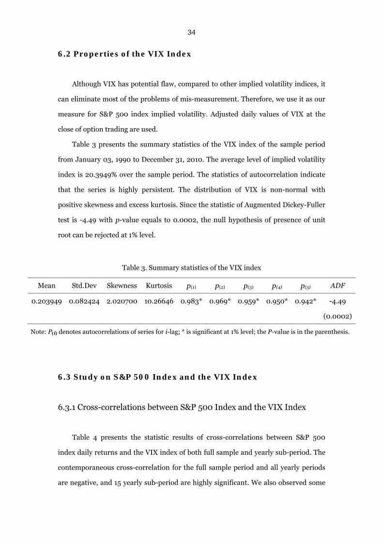
Table 3 presents the summary statistics of the VIX index of the sample period
from January 03, 1990 to December 31, 2010. The average level of implied volatility
index is 20.3949% over the sample period. The statistics of autocorrelation indicate
that the series is highly persistent. The distribution of VIX is non-normal with
positive skewness and excess kurtosis. Since the statistic of Augmented Dickey-Fuller
test is -4.49 with p-value equals to 0.0002, the null hypothesis of presence of unit
root can be rejected at 1% level.
Table 3. Summary statistics of the VIX index
Mean Std.Dev Skewness Kurtosis p(1) p(2) p(3) p(4) p(5) ADF
0.203949 0.082424 2.020700 10.26646 0.983* 0.969* 0.959* 0.950* 0.942* -4.49
(0.0002)
Note: P(i) denotes autocorrelations of series for i-lag; * is significant at 1% level; the P-value is in the parenthesis.
6.3 Study on S&P 500 Index and the VIX Index
6.3.1 Cross-correlations between S&P 500 Index and the VIX Index
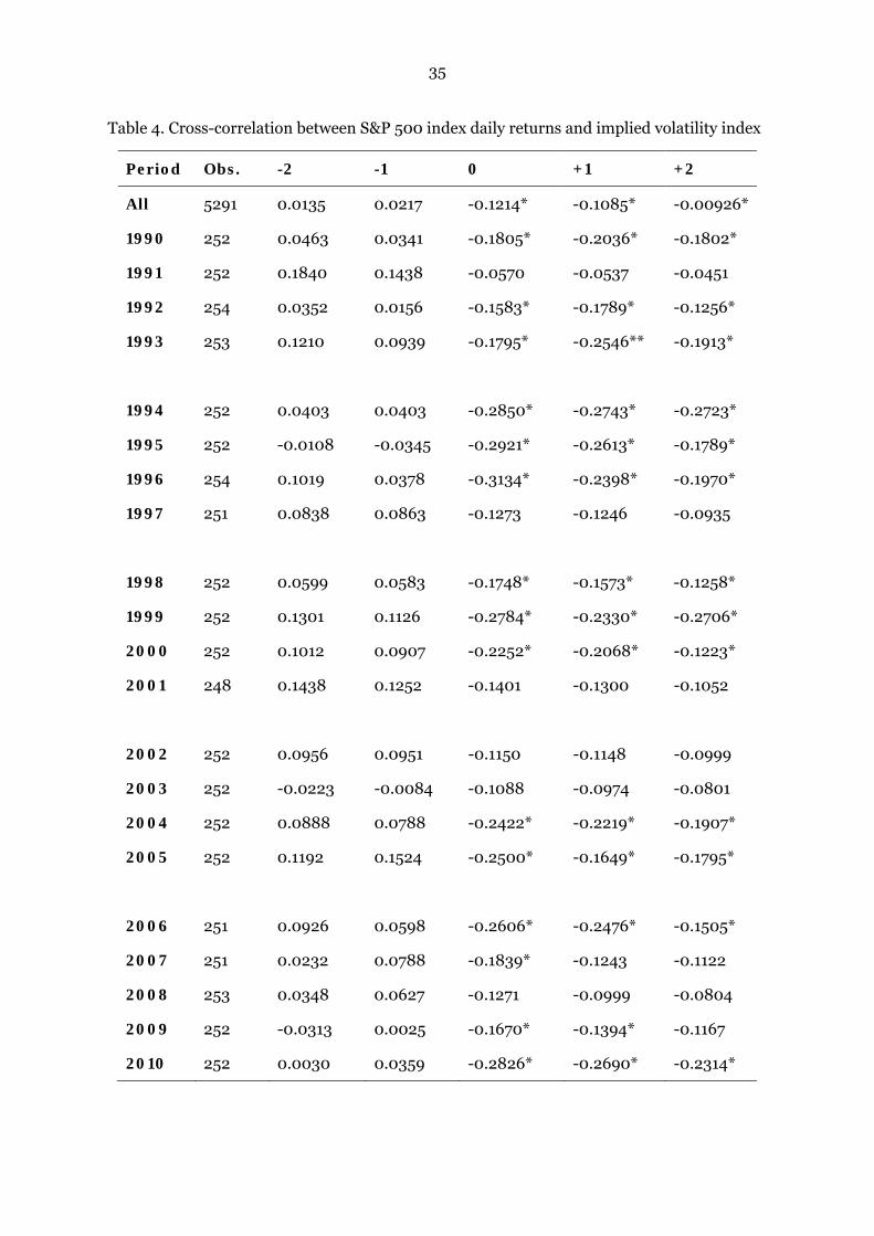
Table 4 presents the statistic results of cross-correlations between S&P 500
index daily returns and the VIX index of both full sample and yearly sub-period. The
contemporaneous cross-correlation for the full sample period and all yearly periods
are negative, and 15 yearly sub-period are highly significant. We also observed some
35
Table 4. Cross-correlation between S&P 500 index daily returns and implied volatility index
Period Obs. -2 -1 0 +1 +2
All 5291 0.0135 0.0217 -0.1214* -0.1085* -0.00926*
1990 252 0.0463 0.0341 -0.1805* -0.2036* -0.1802*
1991 252 0.1840 0.1438 -0.0570 -0.0537 -0.0451
1992 254 0.0352 0.0156 -0.1583* -0.1789* -0.1256*
1993 253 0.1210 0.0939 -0.1795* -0.2546** -0.1913*
1994 252 0.0403 0.0403 -0.2850* -0.2743* -0.2723*
1995 252 -0.0108 -0.0345 -0.2921* -0.2613* -0.1789*
1996 254 0.1019 0.0378 -0.3134* -0.2398* -0.1970*
1997 251 0.0838 0.0863 -0.1273 -0.1246 -0.0935
1998 252 0.0599 0.0583 -0.1748* -0.1573* -0.1258*
1999 252 0.1301 0.1126 -0.2784* -0.2330* -0.2706*
2000 252 0.1012 0.0907 -0.2252* -0.2068* -0.1223*
2001 248 0.1438 0.1252 -0.1401 -0.1300 -0.1052
2002 252 0.0956 0.0951 -0.1150 -0.1148 -0.0999
2003 252 -0.0223 -0.0084 -0.1088 -0.0974 -0.0801
2004 252 0.0888 0.0788 -0.2422* -0.2219* -0.1907*
2005 252 0.1192 0.1524 -0.2500* -0.1649* -0.1795*
2006 251 0.0926 0.0598 -0.2606* -0.2476* -0.1505*
2007 251 0.0232 0.0788 -0.1839* -0.1243 -0.1122
2008 253 0.0348 0.0627 -0.1271 -0.0999 -0.0804
2009 252 -0.0313 0.0025 -0.1670* -0.1394* -0.1167
2010 252 0.0030 0.0359 -0.2826* -0.2690* -0.2314*
36
significant cross-correlations at other leads for various yearly periods but not for any
lags.
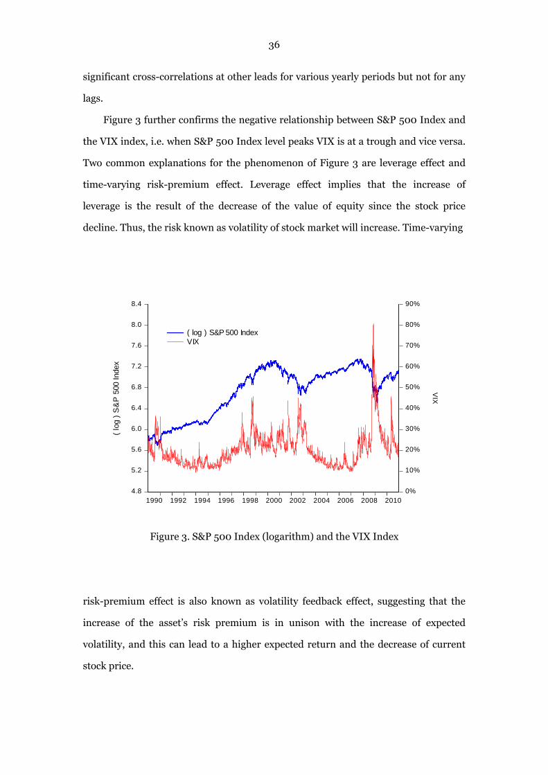
Figure 3 further confirms the negative relationship between S&P 500 Index and
the VIX index, i.e. when S&P 500 Index level peaks VIX is at a trough and vice versa.
Two common explanations for the phenomenon of Figure 3 are leverage effect and
time-varying risk-premium effect. Leverage effect implies that the increase of
leverage is the result of the decrease of the value of equity since the stock price
decline. Thus, the risk known as volatility of stock market will increase. Time-varying
Figure 3. S&P 500 Index (logarithm) and the VIX Index
risk-premium effect is also known as volatility feedback effect, suggesting that the
increase of the asset’s risk premium is in unison with the increase of expected
volatility, and this can lead to a higher expected return and the decrease of current
stock price.
4.8
5.2
5.6
6.0
6.4
6.8
7.2
7.6
8.0
8.4
0%
10%
20%
30%
40%
50%
60%
70%
80%
90%
1990 1992 1994 1996 1998 2000 2002 2004 2006 2008 2010
( log ) S&P 500 IndexVIX
( log
) S
&P
500
Inde
xV
IX

37
6.3.2 S&P 500 Index Daily Returns and the VIX Index
The relationship between stock market returns and implied volatility index was
first investigated by Fleming et al. (1995) for US stock market, and the presence of
significant negative and asymmetric relationship was demonstrated. The VIX index is
widely recognized as an effective proxy for expected volatility. Since VIX was
calculated by the option prices of S&P 100 index before 2003, therefore, it is
interesting to study the contemporaneous relationship between S&P 500 index daily
returns and the VIX index using 21-year historical data, and we want to confirm
whether the relationship between S&P 500 index and its based VIX is still negative
and asymmetric.
By following Fleming et al. (1995), we ran a regression of S&P 500 index daily
returns and contemporaneous daily VIX changes on leads and lags. In order to
evaluate whether there is an asymmetric contemporaneous relationship between S&P
500 index returns and the VIX index, the absolute daily returns at a lag of zero is
included. Additionally, the VIX at a lag of one is also included for controlling for
first-order autocorrelation. The regression has the form:
∆ | | ∆ 29
In line with previous empirical studies by Fleming et al. (1995), Frijns et al.
(2008) and Frijns et al. (2010), the parameter of is expected to be negative. If
is positive and significant, the relationship between S&P 500 index returns and
changes in VIX is asymmetric.
Table 5 presents the regression results for VIX changes and intertemporal S&P
500 index daily returns for the full sample and yearly sub-periods. For the full sample
period, the value of parameter of is same as our expectation. The highly
significant with a t-statistic of -90.43 confirms the negative contemporaneous
relationship between VIX changes and S&P 500 index daily returns. The positive and
significant with t-statistic of 9.62 shows the evidence for asymmetric relationship
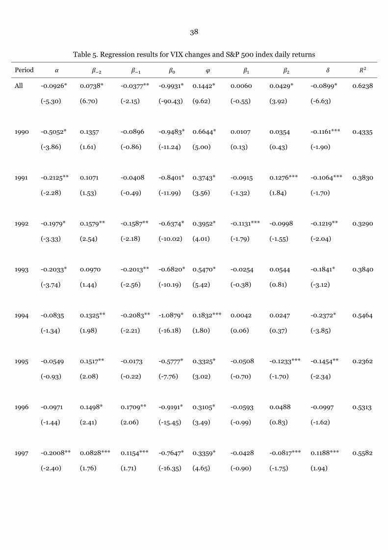
38
Table 5. Regression results for VIX changes and S&P 500 index daily returns
Period
All -0.0926*
(-5.30)
0.0738*
(6.70)
-0.0377**
(-2.15)
-0.9931*
(-90.43)
0.1442*
(9.62)
0.0060
(-0.55)
0.0429*
(3.92)
-0.0899*
(-6.63)
0.6238
1990 -0.5052*
(-3.86)
0.1357
(1.61)
-0.0896
(-0.86)
-0.9483*
(-11.24)
0.6644*
(5.00)
0.0107
(0.13)
0.0354
(0.43)
-0.1161***
(-1.90)
0.4335
1991 -0.2125**
(-2.28)
0.1071
(1.53)
-0.0408
(-0.49)
-0.8401*
(-11.99)
0.3743*
(3.56)
-0.0915
(-1.32)
0.1276***
(1.84)
-0.1064***
(-1.70)
0.3830
1992 -0.1979*
(-3.33)
0.1579**
(2.54)
-0.1587**
(-2.18)
-0.6374*
(-10.02)
0.3952*
(4.01)
-0.1131***
(-1.79)
-0.0998
(-1.55)
-0.1219**
(-2.04)
0.3290
1993 -0.2033*
(-3.74)
0.0970
(1.44)
-0.2013**
(-2.56)
-0.6820*
(-10.19)
0.5470*
(5.42)
-0.0254
(-0.38)
0.0544
(0.81)
-0.1841*
(-3.12)
0.3840
1994 -0.0835
(-1.34)
0.1325**
(1.98)
-0.2083**
(-2.21)
-1.0879*
(-16.18)
0.1832***
(1.80)
0.0042
(0.06)
0.0247
(0.37)
-0.2372*
(-3.85)
0.5464
1995 -0.0549
(-0.93)
0.1517**
(2.08)
-0.0173
(-0.22)
-0.5777*
(-7.76)
0.3325*
(3.02)
-0.0508
(-0.70)
-0.1233***
(-1.70)
-0.1454**
(-2.34)
0.2362
1996 -0.0971
(-1.44)
0.1498*
(2.41)
0.1709**
(2.06)
-0.9191*
(-15.45)
0.3105*
(3.49)
-0.0593
(-0.99)
0.0488
(0.83)
-0.0997
(-1.62)
0.5313
1997 -0.2008**
(-2.40)
0.0828***
(1.76)
0.1154***
(1.71)
-0.7647*
(-16.35)
0.3359*
(4.65)
-0.0428
(-0.90)
-0.0817***
(-1.75)
0.1188***
(1.94)
0.5582
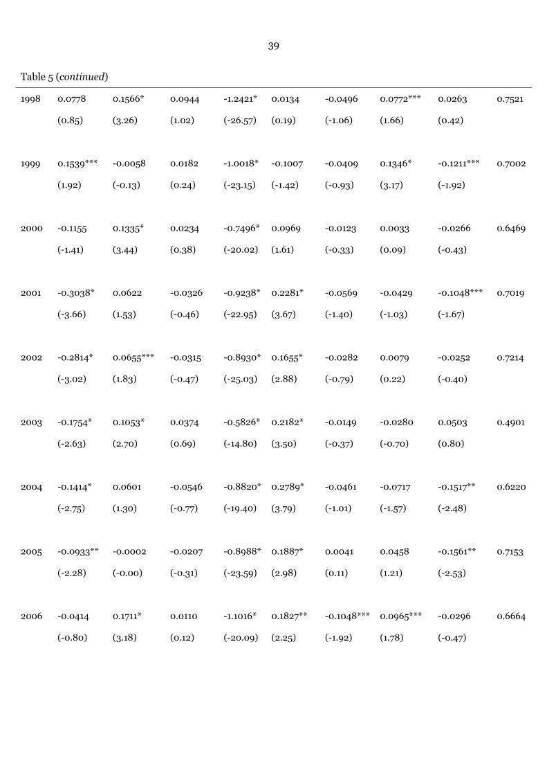
39
Table 5 (continued)
1998 0.0778
(0.85)
0.1566*
(3.26)
0.0944
(1.02)
-1.2421*
(-26.57)
0.0134
(0.19)
-0.0496
(-1.06)
0.0772***
(1.66)
0.0263
(0.42)
0.7521
1999 0.1539***
(1.92)
-0.0058
(-0.13)
0.0182
(0.24)
-1.0018*
(-23.15)
-0.1007
(-1.42)
-0.0409
(-0.93)
0.1346*
(3.17)
-0.1211***
(-1.92)
0.7002
2000 -0.1155
(-1.41)
0.1335*
(3.44)
0.0234
(0.38)
-0.7496*
(-20.02)
0.0969
(1.61)
-0.0123
(-0.33)
0.0033
(0.09)
-0.0266
(-0.43)
0.6469
2001 -0.3038*
(-3.66)
0.0622
(1.53)
-0.0326
(-0.46)
-0.9238*
(-22.95)
0.2281*
(3.67)
-0.0569
(-1.40)
-0.0429
(-1.03)
-0.1048***
(-1.67)
0.7019
2002 -0.2814*
(-3.02)
0.0655***
(1.83)
-0.0315
(-0.47)
-0.8930*
(-25.03)
0.1655*
(2.88)
-0.0282
(-0.79)
0.0079
(0.22)
-0.0252
(-0.40)
0.7214
2003 -0.1754*
(-2.63)
0.1053*
(2.70)
0.0374
(0.69)
-0.5826*
(-14.80)
0.2182*
(3.50)
-0.0149
(-0.37)
-0.0280
(-0.70)
0.0503
(0.80)
0.4901
2004 -0.1414*
(-2.75)
0.0601
(1.30)
-0.0546
(-0.77)
-0.8820*
(-19.40)
0.2789*
(3.79)
-0.0461
(-1.01)
-0.0717
(-1.57)
-0.1517**
(-2.48)
0.6220
2005 -0.0933**
(-2.28)
-0.0002
(-0.00)
-0.0207
(-0.31)
-0.8988*
(-23.59)
0.1887*
(2.98)
0.0041
(0.11)
0.0458
(1.21)
-0.1561**
(-2.53)
0.7153
2006 -0.0414
(-0.80)
0.1711*
(3.18)
0.0110
(0.12)
-1.1016*
(-20.09)
0.1827**
(2.25)
-0.1048***
(-1.92)
0.0965***
(1.78)
-0.0296
(-0.47)
0.6664
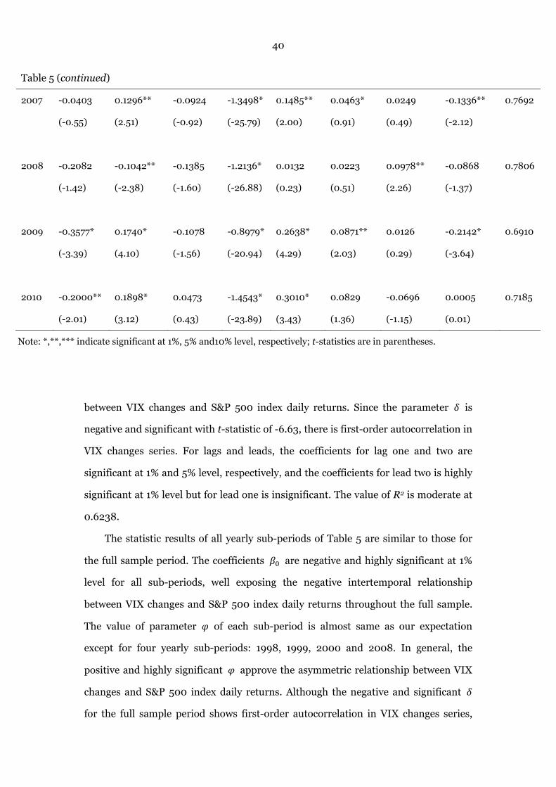
40
Table 5 (continued)
2007 -0.0403
(-0.55)
0.1296**
(2.51)
-0.0924
(-0.92)
-1.3498*
(-25.79)
0.1485**
(2.00)
0.0463*
(0.91)
0.0249
(0.49)
-0.1336**
(-2.12)
0.7692
2008 -0.2082
(-1.42)
-0.1042**
(-2.38)
-0.1385
(-1.60)
-1.2136*
(-26.88)
0.0132
(0.23)
0.0223
(0.51)
0.0978**
(2.26)
-0.0868
(-1.37)
0.7806
2009 -0.3577*
(-3.39)
0.1740*
(4.10)
-0.1078
(-1.56)
-0.8979*
(-20.94)
0.2638*
(4.29)
0.0871**
(2.03)
0.0126
(0.29)
-0.2142*
(-3.64)
0.6910
2010 -0.2000**
(-2.01)
0.1898*
(3.12)
0.0473
(0.43)
-1.4543*
(-23.89)
0.3010*
(3.43)
0.0829
(1.36)
-0.0696
(-1.15)
0.0005
(0.01)
0.7185
Note: *,**,*** indicate significant at 1%, 5% and10% level, respectively; t-statistics are in parentheses.
between VIX changes and S&P 500 index daily returns. Since the parameter is
negative and significant with t-statistic of -6.63, there is first-order autocorrelation in
VIX changes series. For lags and leads, the coefficients for lag one and two are
significant at 1% and 5% level, respectively, and the coefficients for lead two is highly
significant at 1% level but for lead one is insignificant. The value of R2 is moderate at
0.6238.
The statistic results of all yearly sub-periods of Table 5 are similar to those for
the full sample period. The coefficients are negative and highly significant at 1%
level for all sub-periods, well exposing the negative intertemporal relationship
between VIX changes and S&P 500 index daily returns throughout the full sample.
The value of parameter of each sub-period is almost same as our expectation
except for four yearly sub-periods: 1998, 1999, 2000 and 2008. In general, the
positive and highly significant approve the asymmetric relationship between VIX
changes and S&P 500 index daily returns. Although the negative and significant
for the full sample period shows first-order autocorrelation in VIX changes series,
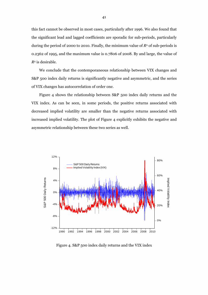
41
this fact cannot be observed in most cases, particularly after 1996. We also found that
the significant lead and lagged coefficients are sporadic for sub-periods, particularly
during the period of 2000 to 2010. Finally, the minimum value of R2 of sub-periods is
0.2362 of 1995, and the maximum value is 0.7806 of 2008. By and large, the value of
R2 is desirable.
We conclude that the contemporaneous relationship between VIX changes and
S&P 500 index daily returns is significantly negative and asymmetric, and the series
of VIX changes has autocorrelation of order one.
Figure 4 shows the relationship between S&P 500 index daily returns and the
VIX index. As can be seen, in some periods, the positive returns associated with
decreased implied volatility are smaller than the negative returns associated with
increased implied volatility. The plot of Figure 4 explicitly exhibits the negative and
asymmetric relationship between these two series as well.
Figure 4. S&P 500 index daily returns and the VIX index
-12%
-8%
-4%
0%
4%
8%
12%
0%
20%
40%
60%
80%
1990 1992 1994 1996 1998 2000 2002 2004 2006 2008 2010
S&P 500 Daily ReturnsImplied Volatility Index (VIX)
Implied V
olatility IndexS&
P 5
00 D
aily
Ret
urns

42
The relationship between S&P 500 index absolute daily returns and the VIX
index are also examined, and the time series plot is presented by Figure 5. It is
obvious that there is close relationship between S&P 500 index absolute daily returns
and VIX because these two time series broadly move in unison during the sample
period. Therefore, VIX performs well for capturing market volatility of S&P 500
index returns.
Figure 5 S&P 500 index absolute daily returns and the VIX index
0%
2%
4%
6%
8%
10%
12%
14%
16%
18%
0%
10%
20%
30%
40%
50%
60%
70%
80%
90%
1990 1992 1994 1996 1998 2000 2002 2004 2006 2008 2010
Implied Volati l i ty Index (VIX)S&P 500 Absolute Daily Returns
S&
P 5
00 A
bsol
ute
Dai
ly R
etur
nsIm
plied Volatility Index

43
7 Estimation and Discussion
This section starts with the study on information criterion which is used for the
selection of orders of ARCH and GARCH terms of various GARCH (p,q) models.
Then, the numerical accuracy of the estimates of GARCH (p,q) models is examined by
comparing the estimates from GARCH (p,q) models to the estimates from ARCH (p)
models. Next, we detailed the coefficient estimates of respective GARCH (p,q) model
as well as the benchmark model (random walk model). In addition, the results of the
standard diagnostics for residuals from the estimated models are also analyzed.
Finally, we provide the study results for the standardized residuals of GARCH (p,q)
models by BDS test and graphical diagnostics.
7.1 Model Selection
The information criterion AIC, SBIC and HQIC of various GARCH (p,q) models
fitted to the daily returns of the S&P 500 index are presented in Table 6. When q=0,
the GARCH (p,q) model reduce to the pure ARCH (p) model.
The information of Panel A indicate that GARCH (4,0) which is equivalent to
ARCH (4) is selected by all information criterions. Panel B shows that GARCH (1,1) is
picked by SBIC and GARCH (2,2) is selected by both AIC and HQIC. For GJR (p,q)
model of Panel C, GJR (2,1) is selected by all information criterions. Finally, the
EGARCH (2,2) is picked by AIC and HQIC but EGARCH (2,1) is preferred by SBIC.
The ultimate column is the log likelihood of each model, and GARCH (4,0), GARCH
(2,2), GJR (2,2) and EGARCH (2,2) models are selected by the maximum value of log
likelihood.
It appears that AIC and HQIC can always provide the same information.
Information criterion is one of criterions for model selection, but it cannot perfectly
indicate whether the model with smallest value of AIC, SBIC or HQIC is the best one.
The performance of an estimated model is affected by many factors. Since the
GARCH (1,1) model is usually assumed to be the best one for modeling and
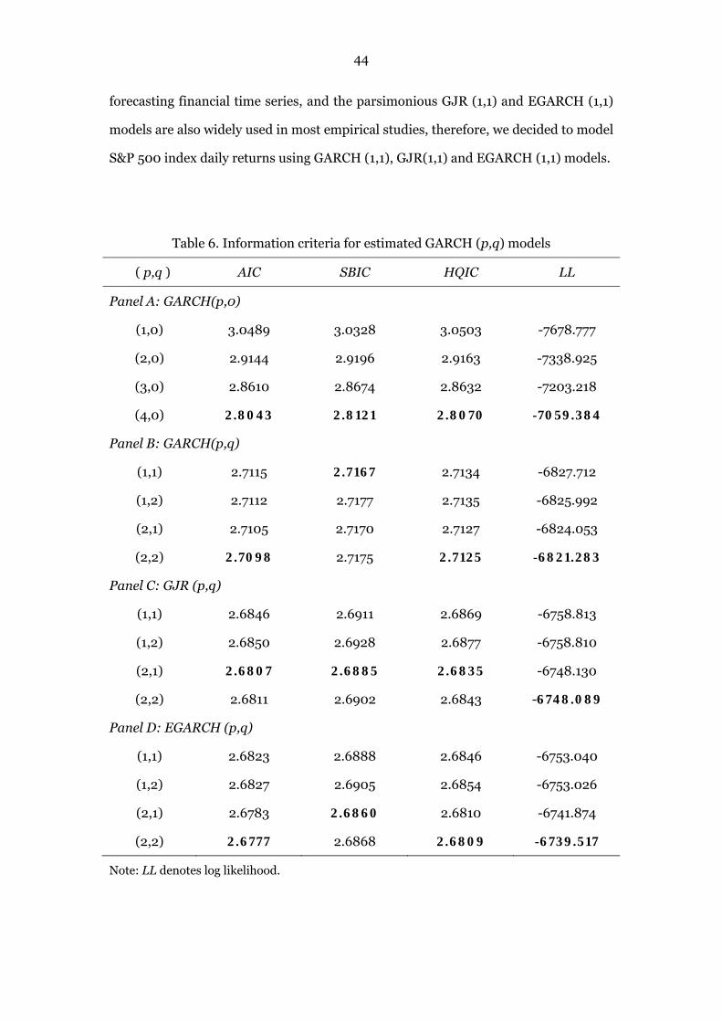
44
forecasting financial time series, and the parsimonious GJR (1,1) and EGARCH (1,1)
models are also widely used in most empirical studies, therefore, we decided to model
S&P 500 index daily returns using GARCH (1,1), GJR(1,1) and EGARCH (1,1) models.
Table 6. Information criteria for estimated GARCH (p,q) models
( p,q ) AIC SBIC HQIC LL
Panel A: GARCH(p,0)
(1,0) 3.0489 3.0328 3.0503 -7678.777
(2,0) 2.9144 2.9196 2.9163 -7338.925
(3,0) 2.8610 2.8674 2.8632 -7203.218
(4,0) 2.8043 2.8121 2.8070 -7059.384
Panel B: GARCH(p,q)
(1,1) 2.7115 2.7167 2.7134 -6827.712
(1,2) 2.7112 2.7177 2.7135 -6825.992
(2,1) 2.7105 2.7170 2.7127 -6824.053
(2,2) 2.7098 2.7175 2.7125 -6821.283
Panel C: GJR (p,q)
(1,1) 2.6846 2.6911 2.6869 -6758.813
(1,2) 2.6850 2.6928 2.6877 -6758.810
(2,1) 2.6807 2.6885 2.6835 -6748.130
(2,2) 2.6811 2.6902 2.6843 -6748.089
Panel D: EGARCH (p,q)
(1,1) 2.6823 2.6888 2.6846 -6753.040
(1,2) 2.6827 2.6905 2.6854 -6753.026
(2,1) 2.6783 2.6860 2.6810 -6741.874
(2,2) 2.6777 2.6868 2.6809 -6739.517
Note: LL denotes log likelihood.
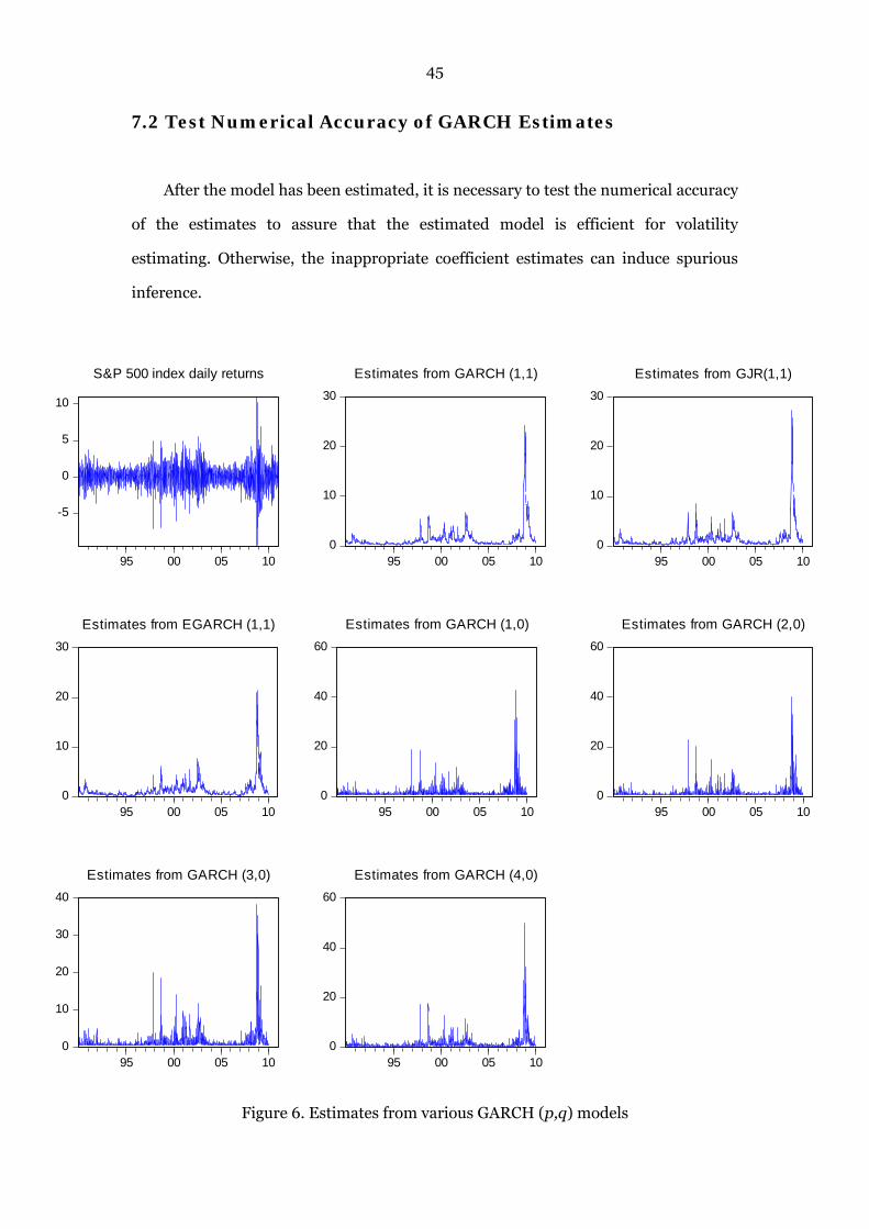
45
7.2 Test Numerical Accuracy of GARCH Estimates
After the model has been estimated, it is necessary to test the numerical accuracy
of the estimates to assure that the estimated model is efficient for volatility
estimating. Otherwise, the inappropriate coefficient estimates can induce spurious
inference.
Figure 6. Estimates from various GARCH (p,q) models
-5
0
5
10
95 00 05 10
S&P 500 index daily returns
0
10
20
30
95 00 05 10
Estimates from GARCH (1,1)
0
10
20
30
95 00 05 10
Estimates from GJR(1,1)
0
10
20
30
95 00 05 10
Estimates from EGARCH (1,1)
0
20
40
60
95 00 05 10
Estimates from GARCH (1,0)
0
20
40
60
95 00 05 10
Estimates from GARCH (2,0)
0
10
20
30
40
95 00 05 10
Estimates from GARCH (3,0)
0
20
40
60
95 00 05 10
Estimates from GARCH (4,0)

46
Zivot (2008) suggests that the numerical accuracy of model estimates can be
examined by comparing the volatility estimates of GARCH (1,1) model with the
volatility estimates from ARCH (p) models. If the volatility estimates from these
different models have the similar dynamics, then the coefficient estimates of models
are appropriate. By following Zivot (2008), we compared the graphical volatility of
GARCH (1,1), GJR (1,1) and EGARCH (1,1) to GARCH (1,0), GARCH (2,0), GARCH
(3,0) and GARCH (4,0) models.
As can be seen from Figure 6, all models perform well in capturing the observed
volatility clustering in S&P 500 index daily returns. In particular, they explicitly
describe the tremendous fluctuation of volatilities of the period from 2007 to 2009,
and this is a concussive financial period experienced the economic prosperity and
economic crisis. Comparing to GARCH (p,0) models ( p=1, 2, 3, 4) which are
equivalent to ARCH(p) models, the volatilities of GARCH(1,1), GJR(1,1) and
EGARCH(1,1) are much smoother and display more persistence. Since the estimated
volatility from these models exhibit the similar dynamics, thus, the estimates of
GARCH (1,1), GJR(1,1) and EGARCH(1,1) models are appropriate.
7.3 Estimates of Models
Table 7 presents the estimates of various models, and they are random walk
model, GARCH (1,1), GJR (1,1) and EGARCH (1,1) models. The second column
presents the estimated parameters and diagnostic results of random walk model. The
coefficient estimate of the constant term is close to zero and statistically insignificant.
The DW statistic shows the result of Durbin-Watson test and it is very close to 2,
suggests that there is no first order autocorrelation of residuals. However, the
Q-statistic and LM statistic from Ljung-box and ARCH-LM tests for the test of lag 10
indicate the presence of autocorrelation.
The coefficient estimates of conditional mean and conditional variance equation
of GARCH (1,1) model are shown in the third column of Table 7. We assumed that the
residuals for the S&P 500 daily returns are normal distributed. The coefficient
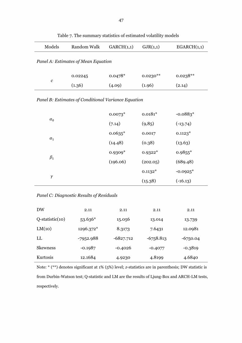
47
Table 7. The summary statistics of estimated volatility models
Models Random Walk GARCH(1,1) GJR(1,1) EGARCH(1,1)
Panel A: Estimates of Mean Equation
c 0.02245 0.0478* 0.0230** 0.0238**
(1.36) (4.09) (1.96) (2.14)
Panel B: Estimates of Conditional Variance Equation
0.0073* 0.0181* -0.0883*
(7.14) (9,85) (-13.74)
0.0635* 0.0017 0.1123*
(14.48) (0.38) (13.63)
0.9309* 0.9322* 0.9855*
(196.06) (202.05) (689.48)
0.1132* -0.0925*
(15.38) (-16.13)
Panel C: Diagnostic Results of Residuals
DW 2.11 2.11 2.11 2.11
Q-statistic(10) 53.636* 15.056 13.014 13.739
LM(10) 1296.372* 8.3173 7.6431 12.0981
LL -7952.988 -6827.712 -6758.813 -6750.04
Skewness -0.1987 -0.4026 -0.4077 -0.3819
Kurtosis 12.1684 4.9230 4.8199 4.6840
Note: * (**) denotes significant at 1% (5%) level; z-statistics are in parenthesis; DW statistic is
from Durbin-Watson test; Q-statistic and LM are the results of Ljung-Box and ARCH-LM tests,
respectively.
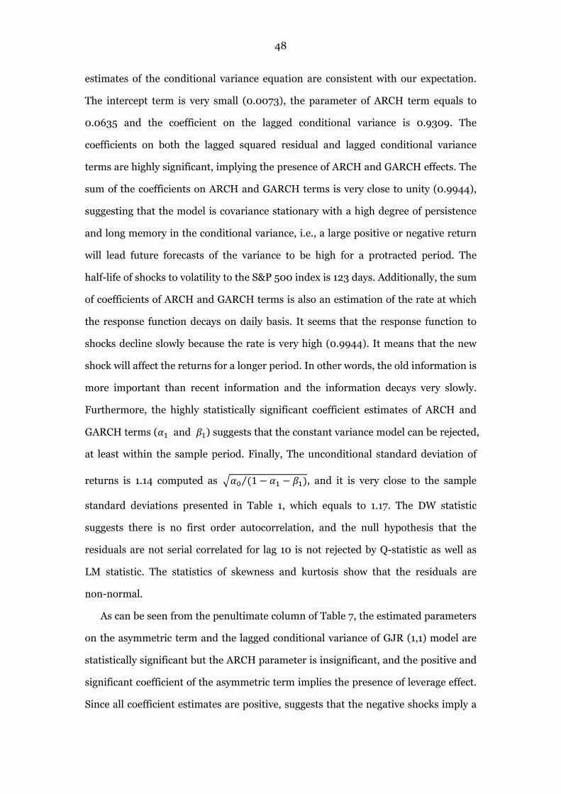
48
estimates of the conditional variance equation are consistent with our expectation.
The intercept term is very small (0.0073), the parameter of ARCH term equals to
0.0635 and the coefficient on the lagged conditional variance is 0.9309. The
coefficients on both the lagged squared residual and lagged conditional variance
terms are highly significant, implying the presence of ARCH and GARCH effects. The
sum of the coefficients on ARCH and GARCH terms is very close to unity (0.9944),
suggesting that the model is covariance stationary with a high degree of persistence
and long memory in the conditional variance, i.e., a large positive or negative return
will lead future forecasts of the variance to be high for a protracted period. The
half-life of shocks to volatility to the S&P 500 index is 123 days. Additionally, the sum
of coefficients of ARCH and GARCH terms is also an estimation of the rate at which
the response function decays on daily basis. It seems that the response function to
shocks decline slowly because the rate is very high (0.9944). It means that the new
shock will affect the returns for a longer period. In other words, the old information is
more important than recent information and the information decays very slowly.
Furthermore, the highly statistically significant coefficient estimates of ARCH and
GARCH terms ( and ) suggests that the constant variance model can be rejected,
at least within the sample period. Finally, The unconditional standard deviation of
returns is 1.14 computed as 1⁄ , and it is very close to the sample
standard deviations presented in Table 1, which equals to 1.17. The DW statistic
suggests there is no first order autocorrelation, and the null hypothesis that the
residuals are not serial correlated for lag 10 is not rejected by Q-statistic as well as
LM statistic. The statistics of skewness and kurtosis show that the residuals are
non-normal.
As can be seen from the penultimate column of Table 7, the estimated parameters
on the asymmetric term and the lagged conditional variance of GJR (1,1) model are
statistically significant but the ARCH parameter is insignificant, and the positive and
significant coefficient of the asymmetric term implies the presence of leverage effect.
Since all coefficient estimates are positive, suggests that the negative shocks imply a
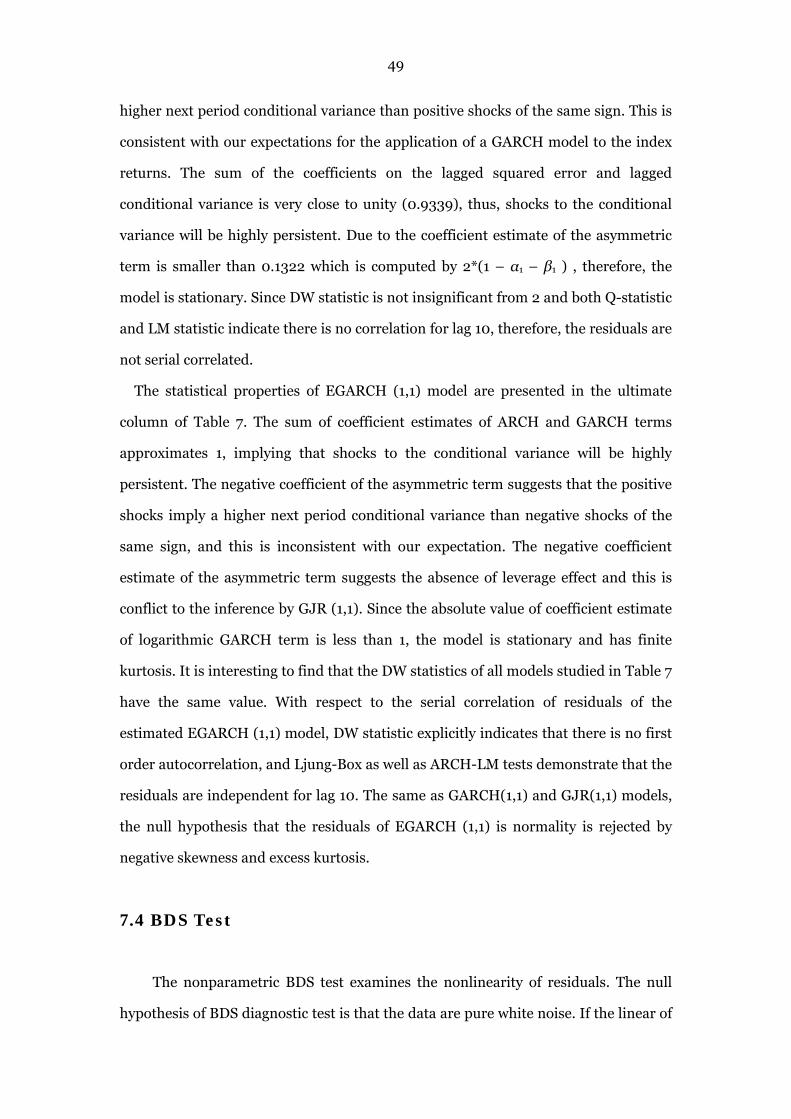
49
higher next period conditional variance than positive shocks of the same sign. This is
consistent with our expectations for the application of a GARCH model to the index
returns. The sum of the coefficients on the lagged squared error and lagged
conditional variance is very close to unity (0.9339), thus, shocks to the conditional
variance will be highly persistent. Due to the coefficient estimate of the asymmetric
term is smaller than 0.1322 which is computed by 2*(1 – α1 – β1 ) , therefore, the
model is stationary. Since DW statistic is not insignificant from 2 and both Q-statistic
and LM statistic indicate there is no correlation for lag 10, therefore, the residuals are
not serial correlated.
The statistical properties of EGARCH (1,1) model are presented in the ultimate
column of Table 7. The sum of coefficient estimates of ARCH and GARCH terms
approximates 1, implying that shocks to the conditional variance will be highly
persistent. The negative coefficient of the asymmetric term suggests that the positive
shocks imply a higher next period conditional variance than negative shocks of the
same sign, and this is inconsistent with our expectation. The negative coefficient
estimate of the asymmetric term suggests the absence of leverage effect and this is
conflict to the inference by GJR (1,1). Since the absolute value of coefficient estimate
of logarithmic GARCH term is less than 1, the model is stationary and has finite
kurtosis. It is interesting to find that the DW statistics of all models studied in Table 7
have the same value. With respect to the serial correlation of residuals of the
estimated EGARCH (1,1) model, DW statistic explicitly indicates that there is no first
order autocorrelation, and Ljung-Box as well as ARCH-LM tests demonstrate that the
residuals are independent for lag 10. The same as GARCH(1,1) and GJR(1,1) models,
the null hypothesis that the residuals of EGARCH (1,1) is normality is rejected by
negative skewness and excess kurtosis.
7.4 BDS Test
The nonparametric BDS test examines the nonlinearity of residuals. The null
hypothesis of BDS diagnostic test is that the data are pure white noise. If the linear of
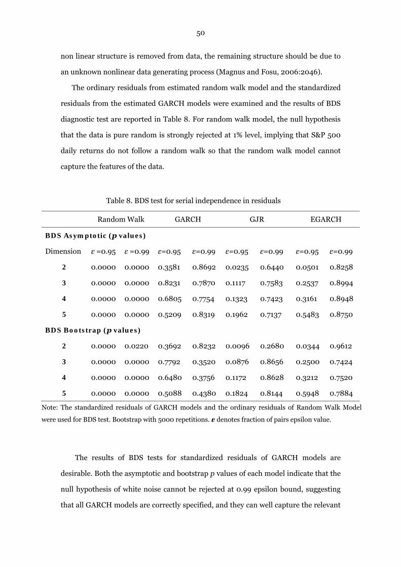
50
non linear structure is removed from data, the remaining structure should be due to
an unknown nonlinear data generating process (Magnus and Fosu, 2006:2046).
The ordinary residuals from estimated random walk model and the standardized
residuals from the estimated GARCH models were examined and the results of BDS
diagnostic test are reported in Table 8. For random walk model, the null hypothesis
that the data is pure random is strongly rejected at 1% level, implying that S&P 500
daily returns do not follow a random walk so that the random walk model cannot
capture the features of the data.
Table 8. BDS test for serial independence in residuals
Random Walk GARCH GJR EGARCH
BDS Asymptotic (p values)
Dimension ε =0.95 ε =0.99 ε=0.95 ε=0.99 ε=0.95 ε=0.99 ε=0.95 ε=0.99
2 0.0000 0.0000 0.3581 0.8692 0.0235 0.6440 0.0501 0.8258
3 0.0000 0.0000 0.8231 0.7870 0.1117 0.7583 0.2537 0.8994
4 0.0000 0.0000 0.6805 0.7754 0.1323 0.7423 0.3161 0.8948
5 0.0000 0.0000 0.5209 0.8319 0.1962 0.7137 0.5483 0.8750
BDS Bootstrap (p values)
2 0.0000 0.0220 0.3692 0.8232 0.0096 0.2680 0.0344 0.9612
3 0.0000 0.0000 0.7792 0.3520 0.0876 0.8656 0.2500 0.7424
4 0.0000 0.0000 0.6480 0.3756 0.1172 0.8628 0.3212 0.7520
5 0.0000 0.0000 0.5088 0.4380 0.1824 0.8144 0.5948 0.7884
Note: The standardized residuals of GARCH models and the ordinary residuals of Random Walk Model
were used for BDS test. Bootstrap with 5000 repetitions. ε denotes fraction of pairs epsilon value.
The results of BDS tests for standardized residuals of GARCH models are
desirable. Both the asymptotic and bootstrap p values of each model indicate that the
null hypothesis of white noise cannot be rejected at 0.99 epsilon bound, suggesting
that all GARCH models are correctly specified, and they can well capture the relevant
51
feature of S&P 500 index daily returns.
Additionally, the insignificant statistic of Ljung-Box and LM test for the
standardized residuals of GARCH models reported in Table 7 show that these models
are successful at modeling the serial correlation structure in the conditional mean
equation and conditional variance equation.
7.5 Graphical Diagnostics
We also examined the standardized residuals of the estimated GARCH models by
graphical diagnostics provided by Figure 7. As can be seen, the autocorrelation
function (ACF) of respective estimated model does not show significant
autocorrelation. The normal qq-plot of the standardized residuals of each estimated
model indicates the strong departures from normality.
In addition, the standard statistical diagnostics of Ljung-Box and Engle’s LM
tests of the estimated GARCH models in Table 7 show the consistent results with ACF
in Figure 7, suggesting that is there is no remaining ARCH effect, and the statistic of
skewness and kurtosis of each estimated model also confirm that the residuals are
non-normal.

52
Figure 7. Graphical residual diagnostics from GARCH (1,1) to S&P 500 returns
-.06
-.04
-.02
.00
.02
.04
.06
5 10 15 20 25 30 35
ACF of standardized residuals from GARCH(1,1)
-4
-2
0
2
4
-8 -4 0 4 8
Quantiles of standardized residuals from GARCH(1,1)
Qua
ntile
s of
Nor
mal
-.06
-.04
-.02
.00
.02
.04
.06
5 10 15 20 25 30 35
ACF of standardized residuals from GJR(1,1)
-4
-2
0
2
4
-8 -4 0 4
Quantiles of standardized residuals from GJR(1,1)
Qua
ntile
s of
Nor
mal
-.06
-.04
-.02
.00
.02
.04
.06
5 10 15 20 25 30 35
ACF of standardized residuals from EGARCH(1,1)
-4
-2
0
2
4
-8 -4 0 4
Quantiles of standardized residuals from EGARCH(1,1)
Qua
ntile
s of
Nor
mal

53
8 Forecast Performance of Estimated Models and VIX
The forecast performance of both time series models and the implied volatility index
(VIX) are discussed in this section. First, the out-of-sample forecast performance of
time series models is examined by the conventional error measurements. Next, the
in-sample forecast performance of implied volatility is studied by running a GARCH
model augmented with dummy variable and exogenous variable. Particularly, the
comparison of forecast performance between VIX, GJR(1,1) and RiskMetrics are
investigated by a variety of approaches.
8.1 out-of-sample Forecast Performance of GARCH Models
The out-of-sample forecast performance of estimated GARCH models are
evaluated by four conventional error measurements, and they are root mean square
error, mean absolute error, mean absolute percentage error and Theil’s U-statistic.
The model with the smallest statistic is considered to be the best for modeling the
conditional volatility of S&P 500 index daily returns.
As can be seen from Table 9, the estimated GARCH(1,1) is considered to be the
best model for out-of-sample forecasting since it has the smallest statistic of RMSE,
MAE and Theil’s U-statistic. If the models are evaluated by MAPE, then GJR (1,1) is
preferred.
Table 9. Forecast Performance of GARCH models
Models GARCH(1,1) GJR(1,1) EGARCH(1,1)
RMSE 1.1355 1.1357 1.1358
MAE 0.7946 0.7964 0.7964
MAPE 122.0995 107.4572 107.8961
Theil 0.9588 0.9795 0.9789

54
Theil’s U-statistics of each model is smaller than one, and this indicates that the
estimated models perform better than the benchmark model. However, the statistic
of MAPE of each model is more than 100%, suggesting that the benchmark model
outperforms the estimated models. Therefore, the result of the comparison between
the estimated models and the random walk model is mixing. It seems MAPE and
Theil’s U-statistic conflict in our test.
Due to the standard GARCH (1,1) cannot capture asymmetry of volatility, and
GJR (1,1) is indicated to be the best one by MAE, thus, GJR (1,1) will be further
studied and its forecast performance will be compared to VIX as well as RiskMetrics
approach.
8.2 In-sample Forecast Performance of VIX
We examined the in-sample forecast performance of VIX by following Blair et al.
(2001) and Frijns et al.(2008) by running the GARCH model augmented with dummy
variable and exogenous variable:
~ 0,
(30)
where denotes S&P 500 index daily return, is the average daily return, is the
random error component on mean level. We assume that is normally distributed
with a mean of zero and a conditional variance equals to . is a dummy variable
which equals to one if the innovation is negative and zero otherwise, and it is used
to capture the asymmetric impact of shocks on volatility.
Six different GARCH specifications are nested by equation (30) if we place
restrictions on it:
(1) if 0, equation (30) becomes a standard GARCH (1,1) model;

55
(2) if 0, equation (30) becomes a GJR (1,1) model which can capturing
asymmetric impact of shocks;
(3) if 0, is the only parameter for explaining the volatility
process;
(4) if 0, then equation (30) becomes a model consisted of VIX and
market shocks;
(5) if 0, then equation (30) includes asymmetry in market shocks;
(6) the equation (30) without any restrictions is a GJR model with implied
volatility which is an exogenous variable.
Table 10. In-sample forecast performance of VIX and GARCH specifications
LL excess LL
GARCH 0.0073* 0.9309* 0.0635* -6827.712
GJR-GARCH 0.0108* 0.9322* 0.0017 0.1103* -6758.813 68.899
VIX -0.5420* 0.0040* -6485.995 341.717
ARCH-VIX -0.0183* -0.0134** 0.0028* -6746.639 81.073
GJR-ARCH-VIX -0.1058* -0.0444* 0.0574* 0.0028* -6740.518 87.194
GJR-GARCH-VIX 0.0008 0.8520* -0.0344* 0.1684* 0.0002* -6703.526 124.186
Note: *(**) denote significant at 1% (5%) level. LL is the statistic of log-likelihood.
The in-sample forecast performance of different models nested in equation (30) are
presented in Table 10, including parameter estimates, the statistics of log-likelihood,
and the values of excess log-likelihood on the basis of the standard GARCH (1,1) in the
second row. The highly significant equals to 0.9309 of GARCH (1,1) model
confirms the strong persistence in volatility. The GJR-GARCH model with
asymmetric term performs better than GARCH (1,1) because the log-likelihood
increase by 69 approximately. Since the estimates of of GJR-GARCH model is
positive, thus the negative shocks imply a higher next period conditional variance.

56
The parameter estimates in the fourth row are for the restricted model which has
0 except for the parameter of . Thus, this model describes the
volatility process only with VIX series, and the large value of excess log-likelihood
(approximate 342) implies that this model performs better than GARCH (1,1). The
nested ARCH-VIX and GJR-ARCH-VIX models incorporate the shock terms into the
specifications, and it is interesting to find that they have the same value of which
equals to 0.0028 and highly significant at 1% level. However, the values of excess
log-likelihood of these two nested models indicate that GJR-ARCH-VIX performs
better, because it has larger excess value compared to the log-likelihood of the
standard GARCH (1,1). In addition, the coefficient of the shock term of
GJR-ARCH-VIX is highly significant at 1% but that of ARCH-VIX is significant at 5%.
The last row shows the estimated parameters of unrestricted model. It is obvious
that GJR-GARCH-VIX significantly improves the standard GARCH (1,1) and it
outperforms GJR-GARCH, ARCH-VIX and GJR-ARCH-VIX, since it has larger excess
log-likelihood. The parameter of is highly significant at 1% level. We also find
that the incorporation of this exogenous variable reduces the value of parameter of the
GARCH term of the standard GARCH (1,1) by approximately 0.08, suggesting that the
VIX series capture a part of persistence in the volatility process.
If comparing all these nested specifications, we find that the addition of VIX can
significantly improve the standard GARCH (1,1). Since the nested VIX model in fourth
row shows the largest excess log-likelihood, thus we conclude that the volatility
process can be reasonably described by VIX series.
8.3 Comparing Predictability of Time Series Models and VIX
In this section, the forecast performance of VIX is investigated as well as
compared to the forecasts performance of RiskMetrics approach and GJR (1,1) models
by running a regression of realized volatility. We consider the forecasting horizons at
5, 10, 15, 30 and 60 trading days. The objective is to investigate whether the VIX
series incorporates all information which has been included in the time series.

57
The time series plots of VIX and annualized future realized volatility over
different horizons are presented by the figures of Appendix A. It seems that VIX can
perfectly track the realized volatility at each horizon. It is obvious that the level of VIX
and realized volatility of each horizon are different, and VIX overestimate the realized
volatility at all horizons. Although the information from figures of Appendix A reveal
that VIX appears to have good forecast performance on realized volatility, we need to
confirm this fact by formal tests of running a regression of realized volatility.
Additionally, we need to investigate whether VIX is superior against other
approaches.
We define the realized volatility as the square root of the sum of S&P 500 index
squared daily returns which is computed as
31
where k denotes the number of trading days, is the squared daily return on day t.
The regression of the realized volatility is given by
, 32
where , denotes forecasts obtained from alternative approaches, and
5, 10, 15, 30, 60 .
In order to run the equation (32),we should primarily construct , series over
different horizons by alternative approaches. By following Giot (2005b) and Frijns et
al. (2008), the k-day forward-looking volatility forecasts on day t by VIX series is
computed as
360 33
58
RiskMetrics approach can be regarded as a simplified and restricted GARCH (1,1)
model. We assume that
1 (34)
where denotes the variance according to RiskMetrics approach, r is return of
S&P 500 index on day t, equals to 0.94 and it captures the persistence of volatility.
Due to the parameters 1 and should sum to one, a unit root is included by
model (51), implying that model (51) is a specific parameterization of Integrated
GARCH (1,1) model. The forecast obtained by model (51) is the forecasts for the next
day. In order to obtain the forecasts for longer horizon, the forecast measurement is
re-scaled and the k-day forward-looking forecast by following Frijns et al. (2008) can
be derived from
· 35
where is the daily forecast by RiskMetrics approach.
The forecasts based on GJR(1,1) model is given by equation (14), and one-day
ahead forward-looking forecast can be obtained by
36
For -day horizon ( 1), the forward-looking forecast can be computed as
0.5 37
The total volatility -day ahead can be derived from

59
, 38
After deriving the forecasts by these three different approaches, we first examine
the correlation between these forecasts and realized volatility at different horizons,
and our purpose is to confirm whether VIX is a better forecaster than other
approaches; then, the forecast performances are evaluated by running the regression
of realized volatility by equation (32). Furthermore, due to our sample data spans a
considerably long period, thus, the realized volatility at each horizon of both
in-sample and out-of-sample period are regressed.
8.3.1 Correlation between Realized Volatility and Volatility Forecasts
The correlation between future realized volatility and volatility forecasts from
respective forecaster at each forecasting horizon are reported in Table 11. It is obvious
that GJR (1,1) has the highest correlation with realized volatility at each horizon. VIX
has higher correlation compared to Riskmetrics approach in most cases except for the
60-day horizon. It is also interesting to find that the correlation between realized
volatility and GJR (1,1) increases for longer horizon. The information observed from
Table 11 implies that GJR (1,1) may performs best on realized volatility forecasting
against VIX and RiskMetrics approach.
Table 11 Correlation between Realized Volatility and Alternative Forecasters
5-day 10-day 15-day 30-day 60-day
VIX 0.7906 0.8141 0.8086 0.7762 0.7039
RiskMetrics 0.7486 0.7808 0.7813 0.7638 0.7135
GJR (1,1) 0.8482 0.9085 0.9311 0.9615 0.9796
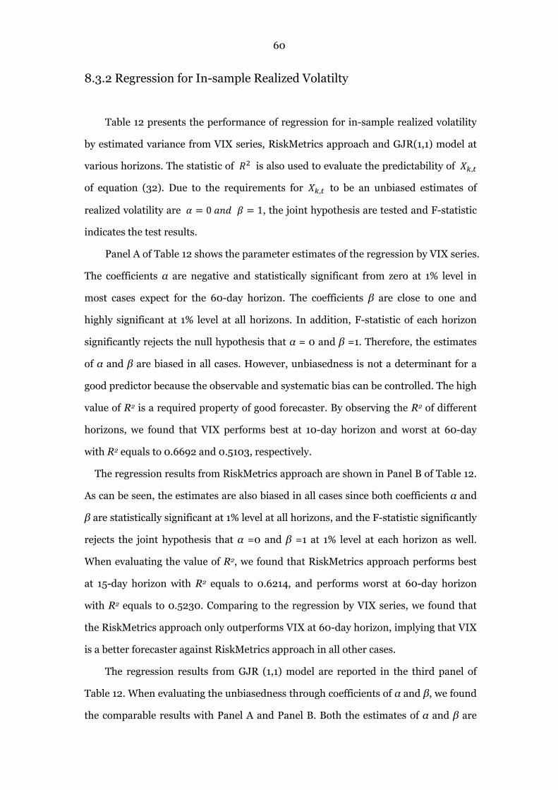
60
8.3.2 Regression for In-sample Realized Volatilty
Table 12 presents the performance of regression for in-sample realized volatility
by estimated variance from VIX series, RiskMetrics approach and GJR(1,1) model at
various horizons. The statistic of is also used to evaluate the predictability of ,
of equation (32). Due to the requirements for , to be an unbiased estimates of
realized volatility are 0 1, the joint hypothesis are tested and F-statistic
indicates the test results.
Panel A of Table 12 shows the parameter estimates of the regression by VIX series.
The coefficients α are negative and statistically significant from zero at 1% level in
most cases expect for the 60-day horizon. The coefficients β are close to one and
highly significant at 1% level at all horizons. In addition, F-statistic of each horizon
significantly rejects the null hypothesis that α = 0 and β =1. Therefore, the estimates
of α and β are biased in all cases. However, unbiasedness is not a determinant for a
good predictor because the observable and systematic bias can be controlled. The high
value of R2 is a required property of good forecaster. By observing the R2 of different
horizons, we found that VIX performs best at 10-day horizon and worst at 60-day
with R2 equals to 0.6692 and 0.5103, respectively.
The regression results from RiskMetrics approach are shown in Panel B of Table 12.
As can be seen, the estimates are also biased in all cases since both coefficients α and
β are statistically significant at 1% level at all horizons, and the F-statistic significantly
rejects the joint hypothesis that α =0 and β =1 at 1% level at each horizon as well.
When evaluating the value of R2, we found that RiskMetrics approach performs best
at 15-day horizon with R2 equals to 0.6214, and performs worst at 60-day horizon
with R2 equals to 0.5230. Comparing to the regression by VIX series, we found that
the RiskMetrics approach only outperforms VIX at 60-day horizon, implying that VIX
is a better forecaster against RiskMetrics approach in all other cases.
The regression results from GJR (1,1) model are reported in the third panel of
Table 12. When evaluating the unbiasedness through coefficients of α and β, we found
the comparable results with Panel A and Panel B. Both the estimates of α and β are
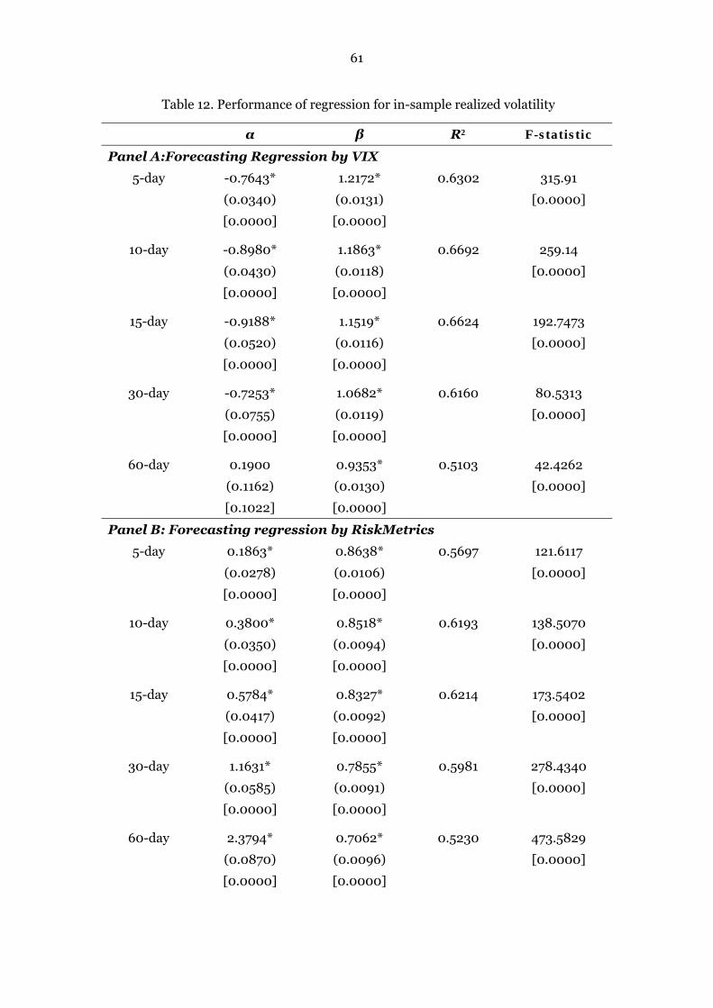
61
Table 12. Performance of regression for in-sample realized volatility
α β R2 F-statistic
Panel A:Forecasting Regression by VIX
5-day -0.7643*
(0.0340)
[0.0000]
1.2172*
(0.0131)
[0.0000]
0.6302 315.91
[0.0000]
10-day -0.8980*
(0.0430)
[0.0000]
1.1863*
(0.0118)
[0.0000]
0.6692 259.14
[0.0000]
15-day -0.9188*
(0.0520)
[0.0000]
1.1519*
(0.0116)
[0.0000]
0.6624 192.7473
[0.0000]
30-day -0.7253*
(0.0755)
[0.0000]
1.0682*
(0.0119)
[0.0000]
0.6160 80.5313
[0.0000]
60-day 0.1900
(0.1162)
[0.1022]
0.9353*
(0.0130)
[0.0000]
0.5103 42.4262
[0.0000]
Panel B: Forecasting regression by RiskMetrics
5-day 0.1863*
(0.0278)
[0.0000]
0.8638*
(0.0106)
[0.0000]
0.5697 121.6117
[0.0000]
10-day 0.3800*
(0.0350)
[0.0000]
0.8518*
(0.0094)
[0.0000]
0.6193 138.5070
[0.0000]
15-day 0.5784*
(0.0417)
[0.0000]
0.8327*
(0.0092)
[0.0000]
0.6214 173.5402
[0.0000]
30-day 1.1631*
(0.0585)
[0.0000]
0.7855*
(0.0091)
[0.0000]
0.5981 278.4340
[0.0000]
60-day 2.3794*
(0.0870)
[0.0000]
0.7062*
(0.0096)
[0.0000]
0.5230 473.5829
[0.0000]

62
Table 12 (continued)
Panel C:Forecasting Regression for GJR(1,1)
5-day -0.2043*
(0.0233)
[0.0000]
1.0250*
(0.0089)
[0.0000]
0.7248 90.7276
[0.0000]
10-day -0.2779*
(0.0247)
[0.0000]
1.0436*
(0.0067)
[0.0000]
0.8292 88.1022
[0.0000]
15-day -0.3350*
(0.0259)
[0.0000]
1.0500*
(0.0057)
[0.0000]
0.8705 99.4965
[0.0000]
30-day -0.4797*
(0.0269)
[0.0000]
1.0604*
(0.0042)
[0.0000]
0.9274 163.9572
[0.0000]
60-day -0.7058*
(0.0278)
[0.0000]
1.0689*
(0.0031)
[0.0000]
0.9605 321.7394
[0.0000]
Note: * denotes significant at 1% level; the statistics of parentheses are standard error; the
statistics of square brackets are P-value; F-statistic are used for the test of joint hypothesis α =
0 and β = 1.
highly significant at 1% level for all cases, and the joint hypothesis α = 0 and β =1 for
each horizon is also explicitly rejected by F-statistic. Therefore, the forecasts by GJR
(1,1) model are also biased forecasts for future volatility at all horizons. However,
comparing to the other two approaches, the coefficients α are more close to zero and
the coefficients β are more close to one at each horizon. With respect to the predictive
power of GJR (1,1) model, the largest value of R2 equaled 0.9605 appears at 60-day
horizon, and the smallest value of R2 equaled 0.7248 is obtained at 5-day horizon. It is
interesting to find that the value of R2 of GJR (1,1) model increases for longer horizon,
and the value of R2 are extremely high at each horizon. It appears that GJR (1,1) has
particular good forecast performance for the long forecasting horizon.

63
To summarize, comparing to VIX series and RiskMetrics approach, GJR (1,1) has
the highest value of R2 and coefficients β are more closer to unity at each horizon.
Consequently, GJR (1,1) model outperforms other approaches on regression for
realized volatility in the sample period, and this finding is consistent with information
observed from Table 11.
We further investigate the out-of-sample forecast performance of each model by
graphical volatility and the conventional error measurements. The figures of
Appendix B plot the out-of-sample volatility forecasts by each model at different
horizons and each model performs well for tracking the dynamics of future volatility.
The statistic of error measures are provided by Table 13, and the information of each
panel explicitly indicates that GJR (1,1) has the best forecast performance for future
realized volatility.
Table 13. Forecast performance on out-of-sample realized volatility
VIX RiskMetrics GJR(1,1)
Panel A: RMSE
5-day 0.8809 1.0256 0.8012
10-day 1.1243 1.2924 0.8287
15-day 1.4051 1.5418 0.8842
30-day 2.2093 2.2978 0.9979
60-day 3.1862 3.1815 0.8467
Panel B: MAE
5-day 0.71956 0.8186 0.6705
10-day 0.8821 1.0238 0.6413
15-day 1.0964 1.1812 0.6837
30-day 1.7227 1.6903 0.7764
60-day 2.6637 2.5519 0.7310
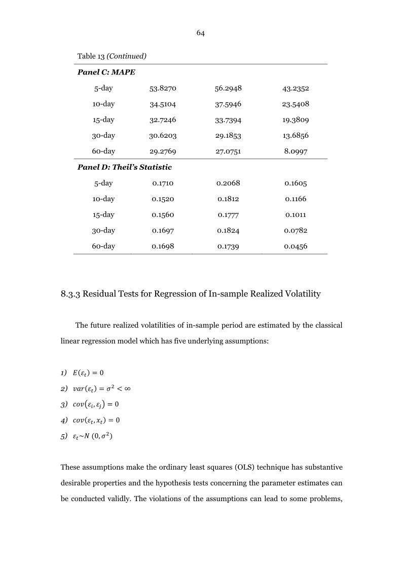
64
Table 13 (Continued)
Panel C: MAPE
5-day 53.8270 56.2948 43.2352
10-day 34.5104 37.5946 23.5408
15-day 32.7246 33.7394 19.3809
30-day 30.6203 29.1853 13.6856
60-day 29.2769 27.0751 8.0997
Panel D: Theil’s Statistic
5-day 0.1710 0.2068 0.1605
10-day 0.1520 0.1812 0.1166
15-day 0.1560 0.1777 0.1011
30-day 0.1697 0.1824 0.0782
60-day 0.1698 0.1739 0.0456
8.3.3 Residual Tests for Regression of In-sample Realized Volatility
The future realized volatilities of in-sample period are estimated by the classical
linear regression model which has five underlying assumptions:
1) 0
2) ∞
3) , 0
4) , 0
5) ~ 0,
These assumptions make the ordinary least squares (OLS) technique has substantive
desirable properties and the hypothesis tests concerning the parameter estimates can
be conducted validly. The violations of the assumptions can lead to some problems,

65
such as both the parameter estimates and the associated standard errors are wrong,
and the distributions assumed for the test statistic are not appropriate.
In order to confirm that the volatility forecasts are efficient and our inferences
based on the coefficient estimates of the regression for in-sample realized volatility
are correct, the residual diagnostic tests were conducted. Due to the coefficients α are
highly significant for all regressions, thus, the first assumption is not violated. In
other words, if a constant is included in the regression model, the first assumption
that the mean of the residuals equals to zero will never be violated. In terms of of
the fourth assumption, it denotes the independent variable of regression equation. If
the independent variable is stochastic and uncorrelated with residual, then the
estimates of OLS are consistent and unbiased.
Table 14 reports the diagnostic results of residuals of regression for in-sample
realilzed volatility. The second column shows the results for heteroskedasticity tests
by the White Test. The autocorrelation of residuals are examined by Durbin-Watson
Test and the results are presented in the third column. The correlation coefficients
between residual and regressor are listed in the fourth column. The statistic of
skewness and kurtosis of the next two columns describe the departures from
normality.
Unfortunately, the diagnostic results are undesirable. The null hypothesis that the
residuals are homoscedastic is explicitly rejected for all regressions at each horizon,
and the DW-statistic of each horizon indicates the presence of first order
autocorrelation of residuals. The correlation coefficients between residuals and
regressors are the same as our expectation. The statistics of skewness and kurtosis
imply that the distributions of residuals are non-normal in all cases. For such a long
in-sample period with 5287 observations, the violation of the normality assumption is
inconsequential.
66
Table 14. Residual tests for regression for in-sample realized volatility
W-statistic DW-statistic Corr( , Skewness Kurtosis
Panel A: Regression by VIX
5-day 689.86
[0.0000]
0.3678 0.0000 1.7703 13.7935
10-day 513.23
[0.0000]
0.1664 0.0000 2.2320 16.4138
15-day 377.04
[0.0000]
0.1294 0.0000 2.7128 21.2689
30-day 178.57
[0.0000]
0.0507 0.0000 3.5227 27.7184
60-day 48.87
[0.0000]
0.0167 0.0000 3.9749 28.3814
Panel B: Regression by RiskMetrics
5-day 559.77
[0.0000]
0.3698 0.0000 1.8001 14.6771
10-day 687.41
[0.0000]
0.1638 0.0000 1.8377 13.9682
15-day 589.31
[0.0000]
0.1397 0.0000 2.0736 16.2758
30-day 284.85
[0.0000]
0.0518 0.0000 2.8501 21.8930
60-day 91.20
[0.0000]
0.0154 0.0000 3.4874 24.0941
Panel A: Regression by GJR (1,1)
5-day 1003.478
[0.0000]
0.4566 0.0000 0.7187 10.9908
10-day 1178.237
[0.0000]
0.2247 0.0000 0.1098 11.3857
15-day 1132.649
[0.0000]
0.2163 0.0000 -0.2153 13.8315
30-day 1150.130
[0.0000]
0.1528 0.0000 -0.2749 15.0022
60-day 1568.914
[0.0000]
0.0464 0.0000 -0.2798 12.9577
Note: W-statistic is the result for heteroskedasticity test by the White Test; DW-statistic is the
result for first order autoccorelation test by the Durbin-Watson Test; Corr( , report the
correlation coefficients between residuals and regressors.

67
8.3.4 Regression for Out-of-sample Realized Volatility
The information observed from Table 14 suggests that the coefficient estimates of
regression for in-sample realized volatility may be wrong so that the inferences based
on analysis of coefficient estimates could be unreliable. In order to further investigate
the predictability of VIX, RiskMetrics and GJR (1,1), we run the OLS regression for
the realized volatility for the out-of-sample period.
Table 15 presents the coefficient estimates of regression for out-of-sample
realized volatility as well as R2 and F-statistic, and the latter one is the result of the
joint hypothesis test. Panel A shows the information of regression by VIX. The
coefficients α are negative at 5-, 10-, and 15-day horizons and they are statistically
significant at 1% level at most horizons except for the 15-day horizon. The estimates of
β are positive and highly significant at 1% level in most cases except for the 60-day
horizon. We also found that the coefficients α increases with longer horizons but the
coefficients β decreases with longer horizons, implying that VIX has weaker
explanatory power for longer horizon. Due to the estimates α is insignificantly from
zero and β is significant and close to one at 15-day horizon, it appears that VIX
performs best for 15-day ahead forecasts. However, F-statistic explicitly rejects the
joint null hypothesis that α = 0 and β = 1. In addition, this joint null hypothesis for
other cases are also rejected by F-statistic. Therefore, the estimates by α and β are
biased. The R2 decreases with longer horizon, suggesting that VIX has better
predictability at the shortest horizon. Our finding regarding performance of VIX
differs from the previous finding based on the regression for in-sample realized
volatility.
Panel B of Table 15 is the results of the regression by RiskMetrics approach of
out-of-sample period. As can be seen, the coefficients α are positive at all horizons and
they are statistically significant in most cases except for the 5-day horizon. The
parameter estimates of β are significant in most cases except for the 60-day horizon.
These findings are comparable with the results of Panel A. Particularly, the estimates
α increases with longer horizons but the estimates of β decreases for longer horizons.
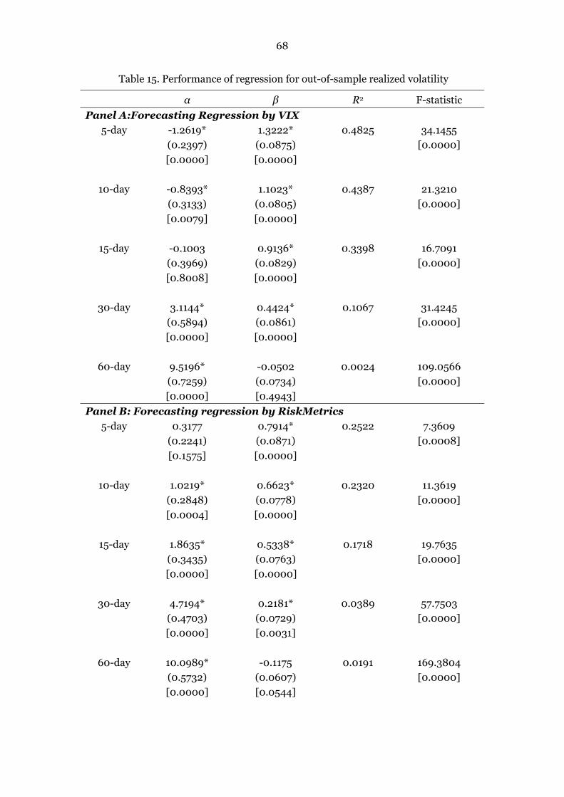
68
Table 15. Performance of regression for out-of-sample realized volatility
α β R2 F-statistic
Panel A:Forecasting Regression by VIX
5-day -1.2619*
(0.2397)
[0.0000]
1.3222*
(0.0875)
[0.0000]
0.4825 34.1455
[0.0000]
10-day -0.8393*
(0.3133)
[0.0079]
1.1023*
(0.0805)
[0.0000]
0.4387 21.3210
[0.0000]
15-day -0.1003
(0.3969)
[0.8008]
0.9136*
(0.0829)
[0.0000]
0.3398 16.7091
[0.0000]
30-day 3.1144*
(0.5894)
[0.0000]
0.4424*
(0.0861)
[0.0000]
0.1067 31.4245
[0.0000]
60-day 9.5196*
(0.7259)
[0.0000]
-0.0502
(0.0734)
[0.4943]
0.0024 109.0566
[0.0000]
Panel B: Forecasting regression by RiskMetrics
5-day 0.3177
(0.2241)
[0.1575]
0.7914*
(0.0871)
[0.0000]
0.2522 7.3609
[0.0008]
10-day 1.0219*
(0.2848)
[0.0004]
0.6623*
(0.0778)
[0.0000]
0.2320 11.3619
[0.0000]
15-day 1.8635*
(0.3435)
[0.0000]
0.5338*
(0.0763)
[0.0000]
0.1718 19.7635
[0.0000]
30-day 4.7194*
(0.4703)
[0.0000]
0.2181*
(0.0729)
[0.0031]
0.0389 57.7503
[0.0000]
60-day 10.0989*
(0.5732)
[0.0000]
-0.1175
(0.0607)
[0.0544]
0.0191 169.3804
[0.0000]

69
Table 15 (continued)
Panel C:Forecasting Regression by GJR(1,1)
5-day -0.2366
(0.1557)
[0.1300]
1.0337*
(0.0607)
[0.0000]
0.5416 4.7423
[0.0095]
10-day -0.1803
(0.1706)
[0.2916]
1.0189*
(0.0467)
[0.0000]
0.6645 2.3019
[0.1023]
15-day -0.1720
(0.1886)
[0.3629]
1.0153*
(0.0420)
[0.0000]
0.7124 1.7324
[0.1791]
30-day -0.0614
(0.7929)
[0.0000]
0.9945*
(0.0363)
[0.0000]
0.7724 1.0366
[0.3564]
60-day -0.0873
(0.2649)
[0.7422]
1.0069*
(0.0284)
[0.0000]
0.8669 0.2236
[0.8942]
Note: * denotes significant at 1% level; P-values are in square brackets.
Additionally, the R2 decreases with longer horizons as well. The same as VIX,
RiskMetrics approach has weaker explanatory power for future volatility for longer
horizon. Comparing to the regression for in-sample realized volatility by RiskMetric
approach, the information of Panel B shows the different performance of RiskMetrics
approach for forecasting out-of-sample realized volatility.
The performance of GJR (1,1) on regressing out-of-sample realized volatility are
presented by the third panel of Table 15. The coefficient estimates α are not
statistically insignificant from zero for all forecasting horizons. The estimates β are
close to one and highly significant at 1% level in all cases. The joint null hypothesis
that α = 0 and β =1 is not rejected by F-statistic at each horizon. Therefore, the
estimates by GJR (1,1) is unbiased and it has strong explanatory power for realized
volatility of the out-of-sample period. The value of R2 at each horizon is much higher
than the R2 of regression by VIX and RiskMetrics, and it increases with longer
70
horizons. Thus, GJR (1,1) has outstanding forecast performance for out-of-sample
realized volatility and outperforms VIX and RiskMetrics. Particularly, GJR (1,1)
performs better for longer forecasting horizon.
To summarize, the information observed from Table 15 demonstrates that the
forecast performance of respective approach on in-sample and out-of-sample realized
volatility is different at each forecasting horizon. However, the study results again
confirms that GJR (1,1) outperforms other approaches.
8.3.5 Residual Tests for Regression of Out-of-sample Realized Volatility
In order to confirm that the inferences based on analysis for information of Table
15 are convincible, the diagnostic tests for residuals of out-of-sample regression are
conducted and the diagnostic results are shown in Table 16. Panel A presents the
diagnostic results of residuals of regression by VIX. The W-statistic of the second
column are the results for heteroscedasticity test. As can be seen, the null hypothesis
that the residuals are homoscedastic is not rejected at 5- and 10-day horizons. The
DW-statistic from Durbin-Watson Test at each horizon indicates the presence of first
order autocorrelation of residuals and the results are undesirable. The correlation
coefficients of residuals and regressors equal to zero at all horizons, suggesting that
the estimates by OLS is consistent and unbiased. The statistic of skewness indicate
that the residuals are positively skewed at all horizons. The kurtosis at each horizon
reveals that the residuals are leptokurtic in most cases but platykurtic at 60-day
horizon. Thus, the normality assumption is violated.
The diagnostic results of Panel B of Table 16 are similar to the results of Panel A.
The residuals of regression by RiskMetrics are homoscedastic at 5- and 10-day
horizons documented by W-statistic of the second column. The presence of first order
autocorrelation of each horizon is confirmed by DW-statistic of the third column. The
residuals are uncorrelated with regressors since the correlation coefficients equal to
zero at each horizon. The normality assumption is violated because the residuals are
positively skewed and leptokurtic in most cases but platykurtic at 60-day horizon.

71
Table 16. Residual tests for regression for out-of-sample realized volatility
W-statistic DW-statistic Corr( , Skewness Kurtosis
Panel A: Regression by VIX
5-day 0.2196
[0.6394]
0.4846 0.0000 0.9849 4.5510
10-day 1.6266
[0.2022]
0.2285 0.0000 1.2872 5.2104
15-day 7.9010
[0.0049]
0.1534 0.0000 1.3408 4.9310
30-day 15.7494
[0.0001]
0.0598 0.0000 0.9751 3.5156
60-day 7.0272
[0.0080]
0.0678 0.0000 0.3166 1.7013
Panel B: Regression by RiskMetrics
5-day 0.0230
[0.8795]
0.4741 0.0000 0.8253 3.9860
10-day 2.3318
[0.1268]
0.2126 0.0000 0.9892 4.0637
15-day 8.2965
[0.0040]
0.1286 0.0000 0.9826 3.7893
30-day 18.9292
[0.0000]
0.0509 0.0000 0.8177 3.1486
60-day 37.7532
[0.0000]
0.0461 0.0000 0.1766 1.5969
Panel C: Regression by GJR(1,1)
5-day 6.4295
[0.0112]
0.7242 0.0000 0.4750 3.1025
10-day 3.5898
[0.0581]
0.3815 0.0000 0.5469 3.7150
15-day 1.9599
[0.1615]
0.1457 0.0000 0.6815 3.7572
30-day 1.9080
[0.1672]
0.1668 0.0000 0.7217 3.4385
60-day 9.3204
[0.0023]
0.2828 0.0000 0.3603 2.0008
Note: W-statistic is the result for heteroskedasticity test by the White Test; DW-statistic is the
result for first order autoccorelation test by the Durbin-Watson Test; Corr( , report the
correlation coefficients between residuals and regressors.
72
Panel C of Table 16 reports the residual tests results of regression by GJR (1,1) for
out-of-sample realized volatility. As can be seen from W-statistic of the second
column, the null hypothesis that the residuals are homoscedastic is not rejected in
most cases except for the 60-day horizon. DW-statistic confirms the first order
autocorrelation of residuals at each horizon. The correlation coefficients of residuals
and regressors show that they are independent of each other in all cases. The
normality assumption is violated since residuals are positively skewed and leptokurtic
in most cases.
The residuals from regression by respective approach at each horizon are plotted
by the figures of Appendix C. The information observed from these figures suggests
that the violation of normality assumption in each case appears to be induced by a
small number of very large positive or negative outliers of each case. Although
DW-statistic of all regressions indicate the presence of first order autocorrelation at
each horizon, the figures of Appendix C show that the residuals have no
autocorrelation over time at 5-, 10- and 15-day horizons, but the residuals are
positively correlated at 30- and 60-day horizons for all regressions.
By and large, the statistics of Table 16 demonstrates that GJR (1,1) performs
better than the other two approaches since the null hypothesis of heteroscedasticity
test is not rejected in most cases and the residuals of GJR (1,1) have a distribution that
is much closer to normality.
8.3.6 Encompassing Regression for Realized Volatility
In the interest of investigating whether the forecast performance of one approach
is superior than the other or whether two approaches complement each other, we run
the encompassing regression followed by Frijns et al. (2008). The form of the
regression is:
, , , 39

73
where , denotes realized volatility at different horizon, , and , are
forecasts from alternative approaches. The significance of and will reveal
whether one approach dominates the other. For instance, if is significant but
is not, it suggests that , performs better than , on future volatility forecasting.
If both and are significant, it implies that these two approaches are
complement each other and each of them has information not included by the other.
Table 17 reports the estimates of encompassing regression at different horizons,
as well as the statistic of R2. Panel A presents the encompassing regression results for
VIX against RiskMetrics approach. Both estimates of β1 and β2 are highly significant
at 1% level with P-values equal to 0.0000. Therefore, VIX and RiskMetrics approach
complement each other, indicating that using both approaches may achieve the best
forecast performance. This can be confirmed if we compare R2 of the regressions for
realized volatility by VIX and RiskMetrics, i.e. the value of R2 of encompassing
regression is larger than R2 of the regression for realized volatility by VIX or
RiskMetrics approach at all horizons.
The forecasting performance of VIX against GJR (1,1) model evaluated by
encompassing regression is presented in the Panel B of Table 17. We found the same
result with Panel A. The estimated parameters of both VIX and variance derived by
GJR (1,1) model at each horizon are highly significant, therefore, VIX and GJR (1,1)
model are complement each other. Since the value of R2 of encompassing regression
for VIX against GJR (1,1) are higher than the value of R2 of Table 15 of regression for
realized volatility by VIX or GJR (1,1) model at each horizon, thus, the joint use of
VIX and the variance from GJR (1,1) model may perform better for future volatility
forecasting.
Panel C of Table 17 shows the regression results for RiskMetrics approach
against GJR (1,1) model. Again, the coefficients of , and , are highly
significant at 1% level with P-values equal to 0.0000 in all cases, and α are negative
and significantly deviate from zero at all horizons. Therefore, the information of
Panel C indicates that RiskMetrics approach and GJR (1,1) model are complement
each other over all forecasting horizons. Comparing to the value of R2 of regression by
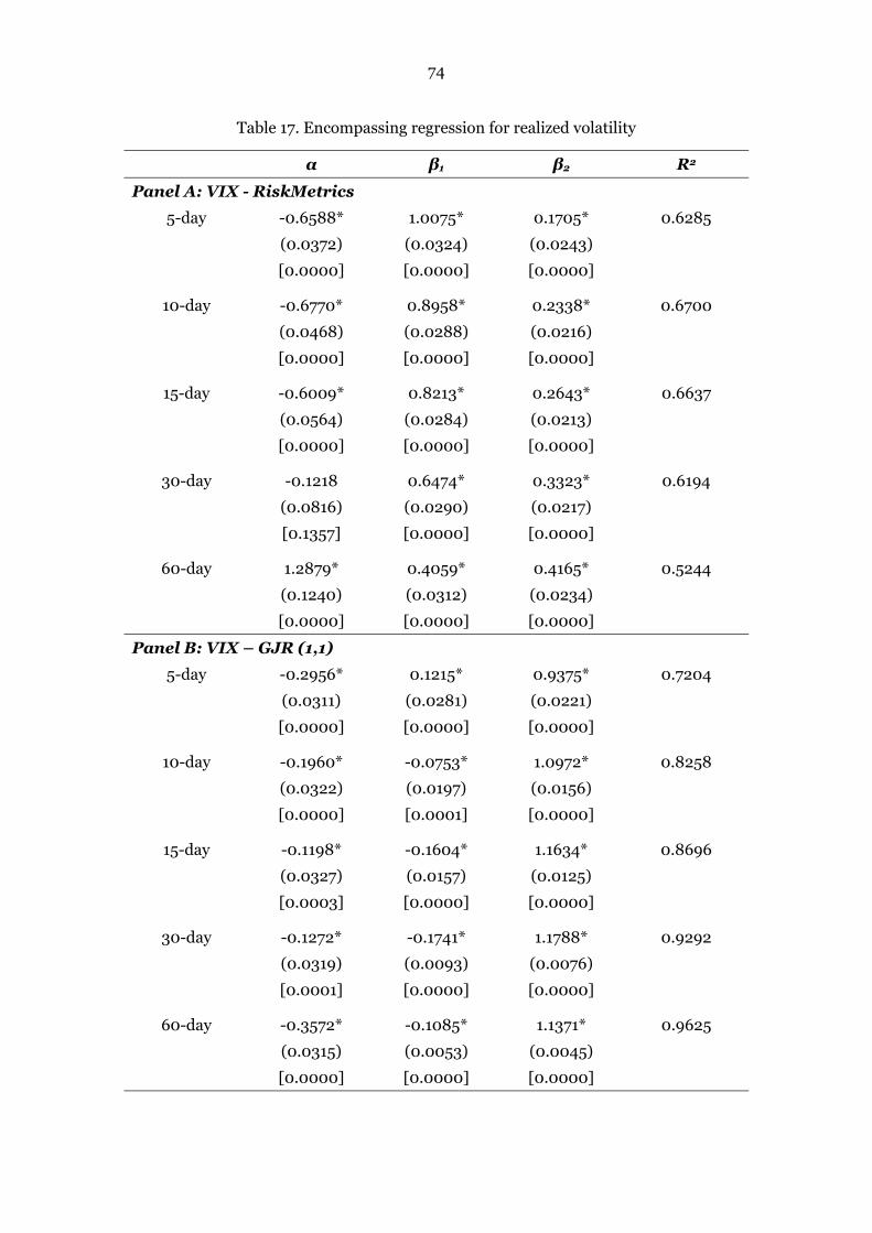
74
Table 17. Encompassing regression for realized volatility
α β1 β2 R2
Panel A: VIX - RiskMetrics
5-day -0.6588*
(0.0372)
[0.0000]
1.0075*
(0.0324)
[0.0000]
0.1705*
(0.0243)
[0.0000]
0.6285
10-day -0.6770*
(0.0468)
[0.0000]
0.8958*
(0.0288)
[0.0000]
0.2338*
(0.0216)
[0.0000]
0.6700
15-day -0.6009*
(0.0564)
[0.0000]
0.8213*
(0.0284)
[0.0000]
0.2643*
(0.0213)
[0.0000]
0.6637
30-day -0.1218
(0.0816)
[0.1357]
0.6474*
(0.0290)
[0.0000]
0.3323*
(0.0217)
[0.0000]
0.6194
60-day 1.2879*
(0.1240)
[0.0000]
0.4059*
(0.0312)
[0.0000]
0.4165*
(0.0234)
[0.0000]
0.5244
Panel B: VIX – GJR (1,1)
5-day -0.2956*
(0.0311)
[0.0000]
0.1215*
(0.0281)
[0.0000]
0.9375*
(0.0221)
[0.0000]
0.7204
10-day -0.1960*
(0.0322)
[0.0000]
-0.0753*
(0.0197)
[0.0001]
1.0972*
(0.0156)
[0.0000]
0.8258
15-day -0.1198*
(0.0327)
[0.0003]
-0.1604*
(0.0157)
[0.0000]
1.1634*
(0.0125)
[0.0000]
0.8696
30-day -0.1272*
(0.0319)
[0.0001]
-0.1741*
(0.0093)
[0.0000]
1.1788*
(0.0076)
[0.0000]
0.9292
60-day -0.3572*
(0.0315)
[0.0000]
-0.1085*
(0.0053)
[0.0000]
1.1371*
(0.0045)
[0.0000]
0.9625

75
Table 17 (continued)
Panel C: RiskMetrics – GJR (1,1)
5-day -0.2123*
(0.0216)
[0.0000]
-0.6575*
(0.0251)
[0.0000]
1.6798*
(0.0263)
[0.0000]
0.7517
10-day -0.2680*
(0.0220)
[0.0000]
-0.5443*
(0.0155)
[0.0000]
1.5789*
(0.0164)
[0.0000]
0.8582
15-day -0.3050*
(0.0225)
[0.0000]
-0.4560*
(0.0116)
[0.0000]
1.4927*
(0.0123)
[0.0000]
0.8972
30-day -0.4047*
(0.0230)
[0.0000]
-0.2872*
(0.0066)
[0.0000]
1.3293*
(0.0072)
[0.0000]
0.9443
60-day -0.5910*
(0.0243)
[0.0000]
-0.1521*
(0.0039)
[0.0000]
1.2027*
(0.0043)
[0.0000]
0.9687
Note: * denotes significant at 1% level; the standard errors are in parentheses;
P-values are in brackets.
each of them in Table 15, we found that the value of R2 of encompassing regression is
much higher. Consequently, the joint use of RiskMetrics approach and GJR (1,1)
model can achieve better forecast performance than using only one of them.
To summarize, we do not find the approach dominating the other by
encompassing regression. The information of the value of R2 observed from each
panel of Table 17 indicate that the forecasting for future volatility by jointly using
RiskMetrics approach and GJR (1,1) model performs best at all horizons.
8.3.7 Average Squared Deviation
Mayhew and Stivers (2003) examined forecast performance of implied volatility
and GARCH type models based on individual stocks by average squared deviation

76
(ASD). The basic idea of ASD approach is to discover the good forecaster by
comparing the average deviation between squared return shocks and estimated
volatility, and the forecaster with the lowest average deviation is considered to be the
best predictor against other approaches. By following Mayhew and Stivers (2003), we
use ASD approach to investigate the forecast performance of VIX, Riskmetrics
approach and GJR (1,1) model at different horizons. The ASD for the volatility
forecast of each model is expressed as:
1 40
where denotes the daily returns, is the average return, T is the number of
observations, and is the out-of-sample conditional variance derived from
alternative model.
Table 18. The average squared deviation from alternative approaches
VIX RiskMetrics GJR (1,1)
ASD 6.1253 6.2622 5.9929
As can be seen from Table 18, GJR (1,1) has the lowest average standard
deviation compared to VIX and RiskMetrics approach, respectively. The information
of Table 18 again documents that GJR (1,1) beats VIX and RiskMetrics approach for
volatility forecasting.
8.3.8 Regression for Squared Return Shocks
We run the regression for squared return shocks by out-of-sample conditional

77
volatility forecasts from VIX, RiskMetrics approach and GJR (1,1) model, respectively.
The objective is to examine which approach can well track the dynamics of daily
volatility. The regression has the form
41
where is the daily return on day t, denotes the average daily return, is the
conditional volatility forecasted by respective approach. The conditions for to be
an unbiased forecaster are α = 0 and β = 1.
Table 19. Regression results for squared return shocks
α β R2
VIX -2.9370*
(-4.4445)
[0.0000]
3.5538*
(6.5669)
[0.0000]
0.1471
RiskMetrics 0.3182
(1.0663)
[0.2873]
0.7427*
(3.8342)
[0.0002]
0.0555
GJR (1,1) 0.1954
(0.7355)
[0.4627]
0.8427*
(5.0624)
[0.0000]
0.0930
Note:* denotes significant at 1% level; t-statistics are in parentheses; P-values are in brackets.
Table 19 reports the parameter estimates for regression of squared return shocks
by out-of-sample volatility forecasts. As can be seen, the coefficient α is negative and
highly significant for regression by VIX, and positive and insignificant in other two
cases. The coefficients β are positive and highly significant at 1% level for all models.
Compared to the regression by VIX, the coefficients β of other two approaches are
more close to unity and the coefficients α are insignificant from zero. However, the
value of R2 of respective approach indicates that VIX outperforms other approaches
outstandingly.

78
8.3.9 Encompassing Regression for Squared Daily Return Shocks
In order to further investigate whether VIX dominates other approaches for
tracking dynamics of daily volatility, we run the encompassing regression for squared
daily return shocks. By following Mayhew and Stivers (2003), the form of the
encompassing regression is:
, , 42
where , is the volatility forecasted by VIX, and , is the volatility forecast from
other approaches.
Table 20. Encompassing regression results for squared return shocks
α β1 β2 R2
VIX-RiskMetrics -4.6452*
(-5.3597)
[0.0000]
6.1189*
(6.0492)
[0.0000]
-1.0265*
(-2.9833)
[0.0031]
0.1766
VIX-GJR(1,1) -5.3426*
(-4.3891)
[0.0000]
6.6711*
(4.6532)
[0.0000]
-1.0026**
(-2.3446)
[0.0198]
0.1655
Note: *, ** denotes significant at 1%, 5% level, respectively; t-statistics are in parentheses;
P-values are in square brackets.
Table 20 presents the parameter estimates of encompassing regression for
squared return shocks by VIX against other approaches, respectively. For regression
by volatility forecasts from VIX and RiskMetrics approach, the coefficient α is
negative and highly significantly deviate from zero, and both the parameter estimates
β1 and β2 are highly significant at 1% level. Therefore, VIX and RiskMetrics approach
are complement each other, suggesting that each of them contains information not
included by the other. For regression by VIX against GJR (1,1), the coefficient α is

79
also negative and highly significant at 1% level, the coefficient β1 is positive and
significant at 1% level, and the coefficient β2 is negative and significant at 5% level.
Consequently, the statistic demonstrates that VIX dominates GJR (1,1) at 1% level,
and these two approaches complement each other at 5% level. In addition, the
parameter estimates of β1 of both encompassing regression indicate that VIX has
stronger positive explanatory power. When evaluating the forecasting ability by the
value of R2 of each regression, the higher R2 of regression by jointly using VIX and
RiskMetrics outperforms the other.

80
9 Conclusion
The objective of this study is to examine the predictive power of model based
forecasts and the VIX index on forecasting future volatility of S&P 500 index daily
returns. The study period is from January 1990 to December 2010, including 5291
observations.
First, a variety of time series models were estimated, including random walk
model, GARCH (1,1), GJR(1,1) and EGARCH (1,1) models. The result of analysis for
the estimated models indicates that GJR (1,1) performs best for out-of-sample
forecast in sample period. Then, the forecast performance of VIX, GJR(1,1) and
RiskMetrics were compared using various approaches by following Frijns et al.(2008),
Giot (2005b) and Mayhew and Stivers (2003). The empirical results are detailed in
section 8.
The results of our study are in line with Becker, Clements and White (2006),
Becker, Clements and White (2007) and Becker and Clements (2008). The empirical
evidence does not support the view that implied volatility subsumes all information
content, and the study results provide strong evidence indicating that GJR (1,1)
outperforms VIX and RiskMetrics for modeling future volatility of S&P 500 index
daily returns. In addition, the results of the encompassing regression for future
realized volatility at 5-, 10-, 15-, 30- and 60-day horizons, and the results of the
encompassing regression for squared return shocks suggest that the joint use of
GJR(1,1) and RiskMetrics can produce the best forecasts.
By and large, our finding indicates that implied volatility is inferior for future
volatility forecasting, and the model based forecasts have more explanatory power for
future volatility.

81
References
Ahoniemi, K. (2006) Modeling and forecasting implied volatility – an econometric
analysis of the VIX index. Helsinki Center of Economic Research, discussion
paper, No.129.
Akgiray, V. (1989). Conditional heteroscedasticity in time series of stock returns:
Evidence and forecasts. Journal of Business, 62, 55-79.
Alexander, C. (2001) Market Models: A guide to financial data analysis. John Wiley
& Sons, Ltd.
Awartani, B. M. A. and Corradi, V. (2005).Predicting the volatility of the S&P-500
stock index via GARCH models: The role of asymmetries. International Journal
of Forecasting, 21, 167-183.
Becker, R. and Clements, A.E. (2008). Are combination forecasts of S&P 500 volatility
statistically superior? International Journal of Forecasting, 24, 122-133.
Becker, R., Clements, A.E. and Coleman-Fenn, C.A. (2009). Forecast performance of
implied volatility and the impact of the volatility risk premium. NCER Working
Paper Series.
http://www.ncer.edu.au/papers/documents/WPNo45.pdf
Becker, R., Clements, A.E. and McClelland, A. (2009). The jump component of S&P
500 volatility and the VIX index. Journal of Banking & Finance, 33, 1033-1038.
Becker, R., Clements, A.E. and White, S.I. (2006). On the informational efficiency of
S&P 500 implied volatility. North American Journal of Economics and Finance,
17, 139-153.
Becker, R., Clements, A.E. and White, S.I. (2007). Does implied volatility provide any
information beyond that captured in model-based volatility forecasts? Journal of
Banking & Finance, 31, 2535-2549.
Blair, B. J., Poon, Ser-H.and Taylor. S. J. (2001). Forecasting S&P 100 volatility: the
incremental information content of implied volatilities and high-frequency index
returns. Journal of Econometrics, 105, 5-26.
Bollerslev, T., Chou, R. Y. and Kroner, K. F. (1992). ARCH modeling in Finance: A
82
review of the theory and empirical evidence. Journal of Econometrics, 52, 1-2,
5-59.
Brailsford, T. J. and Faff, R. W. (1996).An evaluation of volatility forecasting
techniques.Journal of Banking and Finance, 20, 419-438.
Brooks, C. (2008). Introductory Econometrics for Finance.Cambridge University
Press.
Canina, L. and Figlewski, S. (1993). The information content of implied volatility.The
Review of Financial Studies, 6, 3, 659-681.
Chong, C. W., Ahmad, M. I. and Abdullah, M. Y. (1999). Performance of GARCH
models in forecasting stock market volatility. Journal of Forecasting, 18,
333-343.
Christensen, B. J. and Prabhala, N. R., (1998).The relation between implied and
realized volatility. Journal of Financial Economics, 50, 125-150.
Chuang, I. Y., Lu, J. R. and Lee, P. H. (2007). Forecasting volatility in the financial
markets: A comparison of alternative distributional assumptions. Applied
Financial Economics, 17, 1051-1060.
Corrado, C. and Miller, JR.T.W. (2005). The forecast quality of CBOE implied
volatility indexes. The Journal of Futures Markets, 25, 4, 339-373.
Day, T. E. and Lewis, C. M. (1992). Stock market volatility and the information
content of stock index options. Journal of Econometrics, 52, 267-287.
Evans, T. and McMillan, D. G. (2007). Volatility forecasts: The role of asymmetric and
long-memory dynamics and regional evidence. Applied Financial Economics, 17,
1421-1430.
Figlewski, S. (1997). Forecasting volatility. Financial Markets, Institutions and
Instruments, 6,1, 1-88.
Fleming, J., Ostdiek, B. and Whaley, R. E. (1995). Predicting stock market volatility: A
new measure. The Journal of Futures Markets, 15, 3, 265-302.
Franses, P. H. and van Dijk, R. (1996). Forecasting stock market volatility using
(non-linear) GARCH models.Journal of Forecasting, 15, 229-235.
Frijns, B., Tallau, C. and Tourani-Rad, A., (2008). The information content of implied
83
volatility: Evidence from Australia. 21st Australasian Finance and Banking
Conference 2008 Paper.
http://papers.ssrn.com/sol3/papers.cfm?abstract_id=1246142
Frijns, B., Tallau, C. and Tourani-Rad, A., (2010). Australian Implied Volatility Index.
The Finsia Journal of Applied Finance, 1, 31-35.
Galdi, F. C. and Pereira, L. M. (2007). Value at Risk (VaR) using volatility forecasting
models: EWMA, GARCH and Stochastic volatility. Brazilian Business Review, 4,1,
74-94.
Giot, P. (2005a). Relationships between implied volatility indexes and stock index
returns. Journal of Portfolio Management Spring 2005, 31, 3, 92-100.
Giot, P. (2005b). Implied volatility indexes and daily value at risk models. The
Journal of Derivatives, 12, 54-64.
Giot, P. and Laurent, S. (2006). The information content of implied volatility in light
of the jump/continuous decomposition of realized volatility. Working Paper.
http://www.core.ucl.ac.be/econometrics/Giot/Papers/implied4_8.pdf
Harvey, C. R. and Whaley, R. E. (1992). Dividends and S&P 100 Index Option
Valuation. The Journal of Futures Markets, 12, 123-137.
Latané, H. A. and Rendleman, R. J. (1976). Standard deviations of stock price ratios
implied in option prices. The Journal of Finance, 31, 2, 369-381.
Lamoureus, C. G. and Lastrapes, W. D. (1993). Forecasting stock-return variance:
Toward an understanding of stochastic implied volatilities. The Review of
Financial Studies, 6, 2, 293-326.
Lee, J.H.H. and King, M.L. (1993). A locally most powerful based score test for ARCH
and GARCH regression disturbances. Journal of Business and Economic
Statistics, 7, 259-279.
Lumsdaine, R.L. and Ng, S. (1999). Testing for ARCH in the presence of a possibly
misspecified conditional mean. Journal of Econometrics, 93, 257-279.
Magnus, F.J. and Fosu, O.A.E. (2006). Modelling and forecasting volatility of returns
on the Ghana stock exchange using GARCH models. American Journal of
Applied Sciences, 3 (10), 2042-2048.
84
Mayhew, S. and Stivers, C. (2003). Stock return dynamics, option volume, and the
information content of implied volatility. The Journal of Futures Markets, 23, 7,
615-646.
Nelson, D. B. (1992). Filtering and forecasting with misspecified ARCH models I:
getting the right variance with the wrong model. Journal of Econometrics, 52,
61-90.
Patev, P., Kanaryan, N. and Lyroudi, K. (2009). Modelling and forecasting the
volatility of thin emerging stock markets: the case of Bulgaria. Comparative
Economic Research, 12, 4, 47-60.
Poon, S. and Granger, C. (2001). Forecasting financial market volatility: A view.
Working paper, University of Strathclyde and University of California, Sen
Diego.
Poterba, J. M. and Summers, L. H. (1986). The persistence of volatility and stock
market fluctuations. American Economic Review, 76, 1142-1151.
Sheikh, A. M. (1989). Stock splits, volatility increases, and implied volatilities. The
Journal of Finance, 44, 1361-1372.
The CBOE Volatility Index – VIX. (2009). CBOE Proprietary Information. Chicago
Board Options Exchange, Incorporated.
http://www.cboe.com/micro/VIX/vixwhite.pdf
Tse, Y. K. (1991). Stock returns volatility in the Tokyo Stock Exchange. Japan and the
World Economy, 3, 285-298.
Tse, Y. K. and Tung, S. H. (1992). Forecasting volatility in the Singapore stock market.
Asia Pacific Journal of Management, 9(1), 1-13.
Walsh, D. M. and Tsou, G. Y. (1998). Forecasting index volatility: sampling interval
and non-trading effects. Applied Financial Economics, 8, 477-485.
Whaley, R. E. (1993). Derivatives on market volatility: hedging tools long overdue.
Journal of Derivatives, 1,1,71-84.
Wilhelmsson, A. (2006). GARCH forecasting performance under different
distribution assumptions. Journal of Forecasting, 25, 561-578.
Yu, J. (2002). Forecasting volatility in the New Zealand stock market. Applied

85
Financial Economics, 12, 193-202.
Zivot, E. (2008). Practical issue in the analysis of univariate GARCH models.
Handbook of Financial Time Series.

86
Appendix A
VIX and Future Realized Volatility
Figure A.1 VIX and annualized future realized volatility (5 trading days)
Figure A.2 VIX and annualized future realized volatility (10 trading days)
0%
20%
40%
60%
80%
100%
120%
1/1995 1/2000 1/2005 1/2010
Annualized Realized Volatility (5 trading days)VIX
0%
20%
40%
60%
80%
100%
1/1995 1/2000 1/2005 1/2010
Annualized Realized Volatility (10 trading days)VIX

87
Figure A.3 VIX and future realized volatility (15 trading days)
Figure A.4 VIX and annualized future realized volatility (30 trading days)
0%
20%
40%
60%
80%
100%
1/1995 1/2000 1/2005 1/2010
Annualized Realized Volatil ity (15 trading days)VIX
0%
10%
20%
30%
40%
50%
60%
70%
80%
90%
1/1995 1/2000 1/2005 1/2010
Annualized Realized Volatil ity (30 trading days)VIX

88
Figure A.5 VIX and annualized future realized volatility (60 trading days)
0%
10%
20%
30%
40%
50%
60%
70%
80%
90%
1/1995 1/2000 1/2005 1/2010
Annualized Realized Volatil ity (60 trading days)VIX
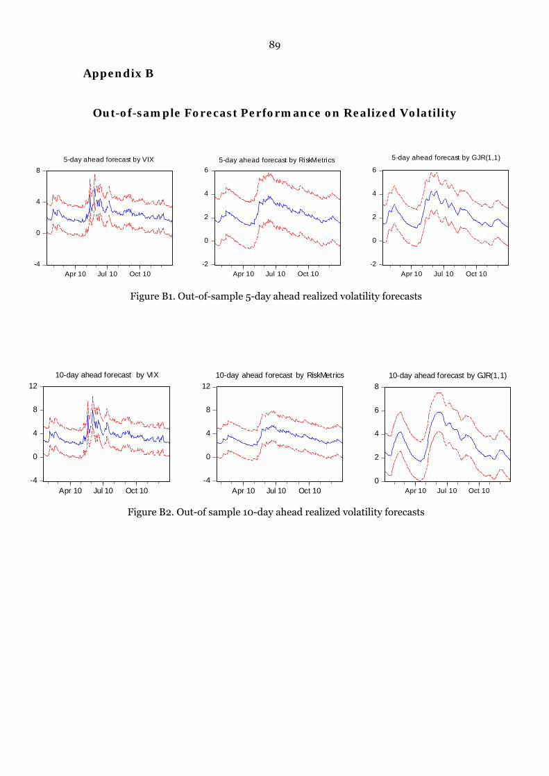
89
Appendix B
Out-of-sample Forecast Performance on Realized Volatility
Figure B1. Out-of-sample 5-day ahead realized volatility forecasts
Figure B2. Out-of sample 10-day ahead realized volatility forecasts
-4
0
4
8
Apr 10 Jul 10 Oct 10
5-day ahead forecast by VIX
-2
0
2
4
6
Apr 10 Jul 10 Oct 10
5-day ahead forecast by RiskMetrics
-2
0
2
4
6
Apr 10 Jul 10 Oct 10
5-day ahead forecast by GJR(1,1)
-4
0
4
8
12
Apr 10 Jul 10 Oct 10
10-day ahead forecast by VIX
-4
0
4
8
12
Apr 10 Jul 10 Oct 10
10-day ahead forecast by RiskMetrics
0
2
4
6
8
Apr 10 Jul 10 Oct 10
10-day ahead forecast by GJR(1,1)
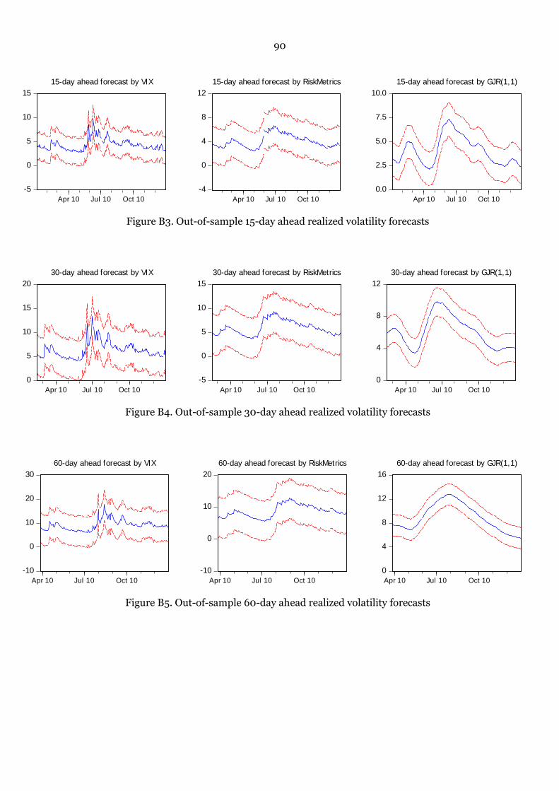
90
Figure B3. Out-of-sample 15-day ahead realized volatility forecasts
Figure B4. Out-of-sample 30-day ahead realized volatility forecasts
Figure B5. Out-of-sample 60-day ahead realized volatility forecasts
-5
0
5
10
15
Apr 10 Jul 10 Oct 10
15-day ahead forecast by VIX
-4
0
4
8
12
Apr 10 Jul 10 Oct 10
15-day ahead forecast by RiskMetrics
0.0
2.5
5.0
7.5
10.0
Apr 10 Jul 10 Oct 10
15-day ahead forecast by GJR(1,1)
0
5
10
15
20
Apr 10 Jul 10 Oct 10
30-day ahead forecast by VIX
-5
0
5
10
15
Apr 10 Jul 10 Oct 10
30-day ahead forecast by RiskMetrics
0
4
8
12
Apr 10 Jul 10 Oct 10
30-day ahead forecast by GJR(1,1)
-10
0
10
20
30
Apr 10 Jul 10 Oct 10
60-day ahead forecast by VIX
-10
0
10
20
Apr 10 Jul 10 Oct 10
60-day ahead forecast by RiskMetrics
0
4
8
12
16
Apr 10 Jul 10 Oct 10
60-day ahead forecast by GJR(1,1)

91
Appendix C
Residuals from Regressions for Out-of-sample Realized Volatility
-2
-1
0
1
2
3
4
4/2010 7/2010 10/2010
Residuals from Regression by VIX (5-day)
-2
0
2
4
6
4/2010 7/2010 10/2010
Residuals from Regression VIX (10-day)
-2
0
2
4
6
4/2010 7/2010 10/2010
Residuals from Regression by RiskMetrics (5-day)
-4
-2
0
2
4
6
4/2010 7/2010 10/2010
Residuals from Regression by RiskMetrics (10-day)
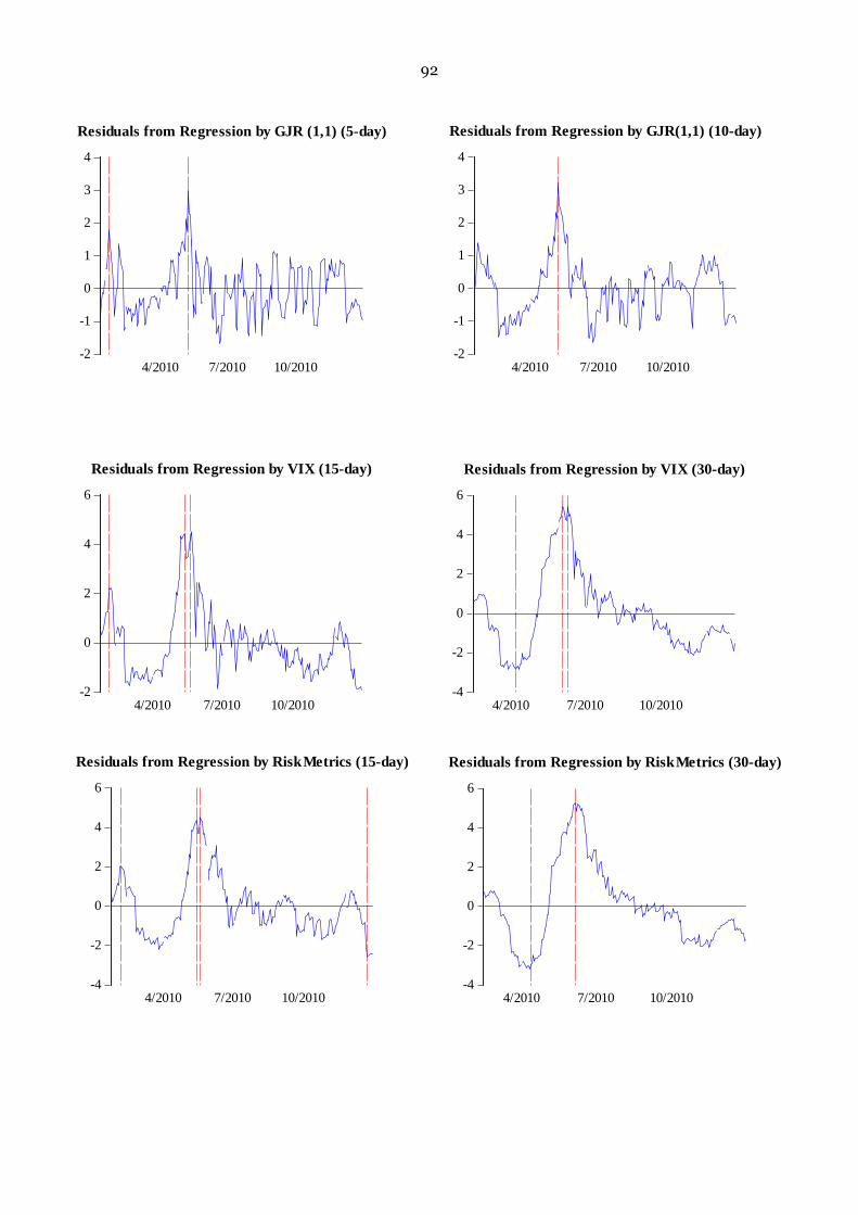
92
-2
-1
0
1
2
3
4
4/2010 7/2010 10/2010
Residuals from Regression by GJR (1,1) (5-day)
-2
-1
0
1
2
3
4
4/2010 7/2010 10/2010
Residuals from Regression by GJR(1,1) (10-day)
-2
0
2
4
6
4/2010 7/2010 10/2010
Residuals from Regression by VIX (15-day)
-4
-2
0
2
4
6
4/2010 7/2010 10/2010
Residuals from Regression by VIX (30-day)
-4
-2
0
2
4
6
4/2010 7/2010 10/2010
Residuals from Regression by RiskMetrics (15-day)
-4
-2
0
2
4
6
4/2010 7/2010 10/2010
Residuals from Regression by RiskMetrics (30-day)

93
-2
-1
0
1
2
3
4
4/2010 7/2010 10/2010
Residuals from Regression by GJR(1,1) (15-day)
-3
-2
-1
0
1
2
3
4/2010 7/2010 10/2010
Residuals from Regression by GJR(1,1) (30-day)
-4
-2
0
2
4
6
4/2010 7/2010 10/2010
Residuals from Regression by VIX (60-day)
-4
-2
0
2
4
4/2010 7/2010 10/2010
Residuals from Regression by RiskMetrics (60-day)
-2
-1
0
1
2
4/2010 7/2010 10/2010
Residuals from Regression by GJR(1,1) (60-day)
Top Related