


Languages
Pages
Legal


1
MODELING THE ECONOMICS OF BIODIVERSITY AND ENVIRONMENTAL
HETEROGENEITY
William Brock University of Wisconsin – Madison Department of Economics 1180 Observatory Drive Madison , WI 53706 United States [email protected] Ann Kinzig School of Life Sciences Arizona State University PO Box 874501 Tempe AZ 85287 USA [email protected] Charles Perrings School of Life Sciences Arizona State University PO Box 874501 Tempe AZ 85287 USA [email protected]
Correspondence to:
Charles Perrings School of Life Sciences Arizona State University PO Box 874501 Tempe AZ 85287 USA [email protected] Tel: 480 727 0472
Fax: 480 965 8087

2
Abstract
It has long been recognized that major drivers of biodiversity loss include both the
harvest of wild species and the conversion of habitat for productive purposes. While
habitat conversion explains a large part of the decline in native species occurring in wild
refugia, however, it ignores the impact of land use in the rest of the landscape. We
address the problem of anthropogenic biodiversity loss across the whole landscape by
modelling the connection between landscape heterogeneity, harvest intensity and the
level of biodiversity. If the system is extremely homogeneous, it is assumed that forces of
competitive exclusion will lead to a single surviving species. If the system is extremely
heterogeneous, it is assumed that multiple species can coexist, with each species
exclusively dominating the patch type to which it is best suited. Alongside the effects of
harvest/pest control, we consider the effect of land use on environmental heterogeneity,
and through that on species richness. We identify the externalities associated with each
activity and the potential for applying corrective measures.
JEL Classification: Q21.
Keywords: Biodiversity, environmental heterogeneity, externality
1. Posing the problem
The impact of economic activity on biodiversity has been evaluated from a number of
perspectives. The most compelling arguments address the link between economic activity
and the loss of natural habitats (e.g. Barbier and Schultz, 1997; Wilcove et al, 1998;
Polasky et al, 2004). Using the species-area relationship (Macarthur and Wilson, 1967),
such studies calculate the impact of economic activity on biodiversity from the proportion

3
of the land area that is converted to other uses, usually to agriculture or forestry. By
assumption, the converted area is lost as natural habitat, and is no longer available to
support species. The number of species that can continue to be supported is therefore
reduced.
While this approach has much to say about species loss in diminishing wildlife refugia,
however, it has little to say about species loss or persistence in the rest of the landscape.
Species can persist in human managed or dominated landscapes, though the species-area
approach described above assumes they cannot. Given the increasing human domination
of the biosphere, understanding how human activities alter biodiversity in worked and
altered landscapes is of growing importance (Perrings and Gadgil, 2003; Daily et al,
2000) and the consequences this has not just for the existence of species, but for the
effects on ecosystem functioning (Hooper et al, 2005; Naeem and Wright, 2003) and the
production of a range of ecosystem services and disservices (Millennium Ecosystem
Assessment, 2005; Barbier, 2007; Barbier et al, forthcoming; Perrings et al, forthcoming).
This poses a different modeling challenge. In this paper, we focus on one particular
ecological explanation of species richness – the heterogeneity of the landscape. This is
also related to land use, but unlike the conversion of habitats it addresses the causes and
consequences of biodiversity change not only in refugia, but across the whole landscape.
We are interested in the relationship between environmental heterogeneity, the intensity
with which species are harvested (or culled), and species diversity. Environmental
heterogeneity in this case refers to the ‘patchiness’ of the landscape, and is taken to be a

4
function of land use or the way that species are exploited. A heterogeneous landscape is
one in which distinct patches favor the existence of distinct species. While competitive
exclusion will reduce diversity in each patch, a high degree of heterogeneity between
patches leads to a high level of species diversity (Kinzig et al, 1999). Biodiversity – in
this case measured by both environmental heterogeneity and species richness – is a
function of the level of economic activity. Species richness may be reduced in two ways:
through ‘harvest’ and through reduced environmental heterogeneity. We show that where
the user cost of individual species is ignored, the privately optimal level of effort and
hence the privately optimal level of environmental heterogeneity will diverge from the
socially optimal level of effort and the socially optimal level of environmental
heterogeneity. We note that harvest effort comprises both the extraction of desirable
species and the control or removal of undesirable species. This is, to our knowledge, the
first attempt to understand the interactions between environmental heterogeneity and
species loss in the context of an economic model.
2. Modeling the relationship between species richness and environmental
heterogeneity
Consider the growth of the ith of m species. Suppressing time arguments, the equation of
motion for this species takes the form:
[1] ( )( ) ( )
( )( )1 ..1 ii
i i i i ii
e L Se L sds s r d adt K m e L Kϕ
⎡ ⎤⎛ ⎞⎛ ⎞⎛ ⎞−⎢ ⎥⎜ ⎟⎜ ⎟= − + − −⎜ ⎟⎜ ⎟⎜ ⎟⎢ ⎥⎜ ⎟⎝ ⎠⎝ ⎠⎝ ⎠⎣ ⎦
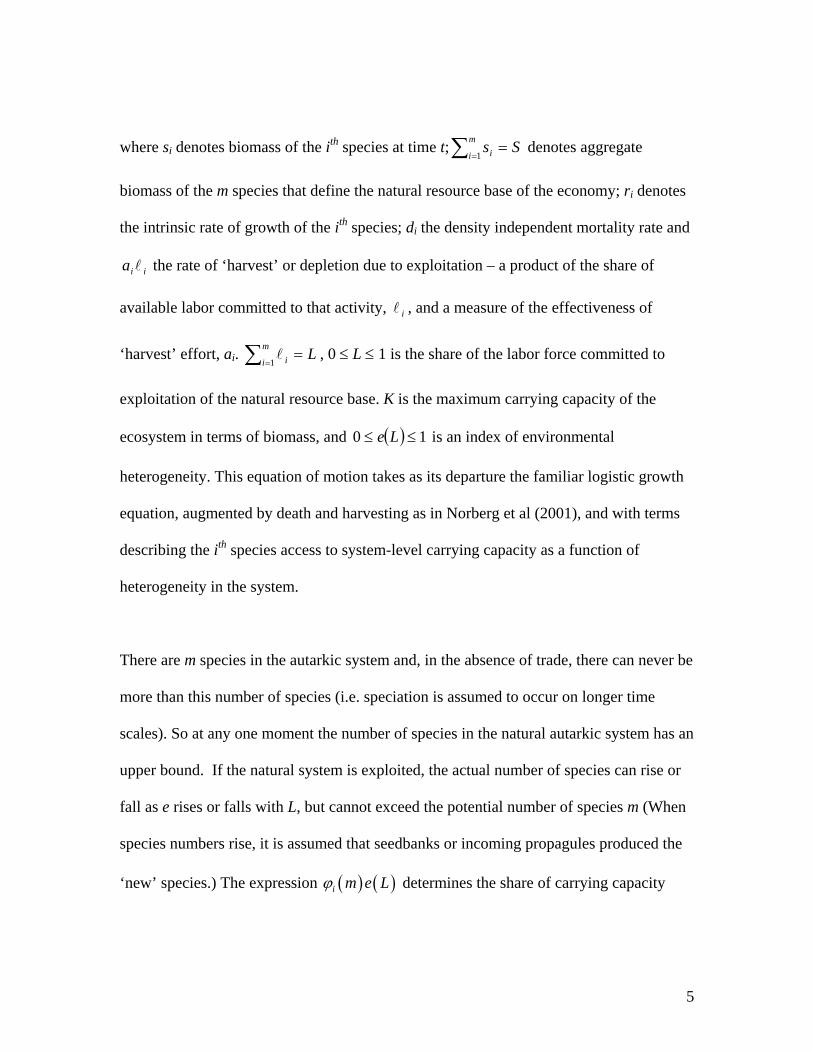
5
where si denotes biomass of the ith species at time t; Ssm
i i =∑ =1 denotes aggregate
biomass of the m species that define the natural resource base of the economy; ri denotes
the intrinsic rate of growth of the ith species; di the density independent mortality rate and
iia the rate of ‘harvest’ or depletion due to exploitation – a product of the share of
available labor committed to that activity, i , and a measure of the effectiveness of
‘harvest’ effort, ai. Lm
i i =∑ =1, 0 ≤ L ≤ 1 is the share of the labor force committed to
exploitation of the natural resource base. K is the maximum carrying capacity of the
ecosystem in terms of biomass, and ( ) 10 ≤≤ Le is an index of environmental
heterogeneity. This equation of motion takes as its departure the familiar logistic growth
equation, augmented by death and harvesting as in Norberg et al (2001), and with terms
describing the ith species access to system-level carrying capacity as a function of
heterogeneity in the system.
There are m species in the autarkic system and, in the absence of trade, there can never be
more than this number of species (i.e. speciation is assumed to occur on longer time
scales). So at any one moment the number of species in the natural autarkic system has an
upper bound. If the natural system is exploited, the actual number of species can rise or
fall as e rises or falls with L, but cannot exceed the potential number of species m (When
species numbers rise, it is assumed that seedbanks or incoming propagules produced the
‘new’ species.) The expression ( ) ( )i m e Lϕ determines the share of carrying capacity
6
accessed by the ith species. This depends on degree of heterogeneity of the landscape and
the number of competing species in the system.
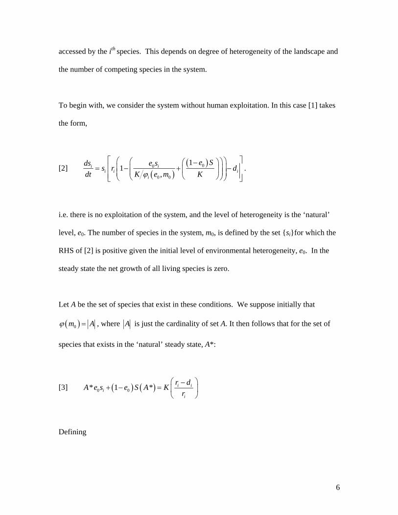
To begin with, we consider the system without human exploitation. In this case [1] takes
the form,
[2] ( )
( )00
0 0
11
,i i
i i ii
e Sds e ss r ddt K e m Kϕ
⎡ ⎤⎛ ⎞⎛ ⎞⎛ ⎞−⎢ ⎥= − + −⎜ ⎟⎜ ⎟⎜ ⎟⎜ ⎟⎜ ⎟⎢ ⎥⎝ ⎠⎝ ⎠⎝ ⎠⎣ ⎦
.
i.e. there is no exploitation of the system, and the level of heterogeneity is the ‘natural’
level, e0. The number of species in the system, m0, is defined by the set {si}for which the
RHS of [2] is positive given the initial level of environmental heterogeneity, e0. In the
steady state the net growth of all living species is zero.
Let A be the set of species that exist in these conditions. We suppose initially that
( )0m Aϕ = , where A is just the cardinality of set A. It then follows that for the set of
species that exists in the ‘natural’ steady state, A*:
[3] ( ) ( )0 0* 1 * i ii
i
r dA e s e S A Kr
⎛ ⎞−+ − = ⎜ ⎟
⎝ ⎠
Defining

7
[4] ⎟⎟⎠
⎞⎜⎜⎝
⎛ −=
i
iii r
drKg :
to be the maximum potential biomass of the ith species in the ‘natural’ state, we can
readily see the implications of environmental heterogeneity for the existence and
abundance of species in the system.
Let the m0 potential species in the system be labeled such that
0 01 2 1 0m mg g g g−> > > > > . Biologically, this tells us that species are competitively
ranked by their equilibrium abundance, implying that they are K-selected (K-strategists
outcompete r-strategists). A necessary though not generally sufficient condition for the
existence of the ith species is that gi > 0: that it’s net growth rate is positive. A sufficient
condition is that:
[5] ( ) [ ]( ) ( )0 10 0
1 ,1, 1
i ki i i k
gg e g gi e i eϕ=
> − =+ −∑
where [1,i] is the interval of indices between 1 and i . The sum is over the set of species
whose equilibrium abundance is not less than that of the ith species, and [ ]( )i,1φ is
evaluated on this set of species. For our leading special case [ ]( ) ii =,1φ and ig is the
average for that case. Note that [5] holds a fortiori for any set of m species, where
0m m i≥ ≥ . That is:

8
[6] ( ) [ ]( ) ( )0 10 0
1 ,1, 1
i ki i i k
gg e g gm e i eϕ=
> − =+ −∑
In the case just considered, A* is an interval A* = [1,m]. Note that, from [3],
[7] [ ]( ) ( )( )0
0
1 11,i is g e S
m eϕ= − −
where S is the aggregate biomass of the set of all living species, and [ ]( )m,1φ is evaluated
on that set. For the special case where A* = [1,m]:
[8] [ ]( ) ( ) ( )( )01 1 1
0
1 11,
m m mi i i ii i i
s K m d r m e sm eϕ= = =
= − − −∑ ∑ ∑
which yields:
[9] ( )
[ ]( ) ( )1
10 01, 1
mi im i
ii
K m d rs
m e m eϕ=
=
−=
+ −
∑∑
Substitution into [6] implies that
[10] [ ]( ) ( )
( )[ ]( ) ( )
10
0 0 0
1 11, 1, 1
mi ii
i i
K m d rs g e
m e m e m eϕ ϕ=
⎛ ⎞⎛ ⎞−⎜ ⎟⎜ ⎟= − −⎜ ⎟⎜ ⎟+ −⎜ ⎟⎜ ⎟⎝ ⎠⎝ ⎠
∑, i = 1,2,…,m

9
For si > 0 it follows that:
[11] ( )( )
[ ]( ) ( )1
00 0
11, 1
mi ii
i
K m d rg e
m e m eϕ=
⎛ ⎞−⎜ ⎟> − ⎜ ⎟+ −⎜ ⎟⎝ ⎠
∑, i = 1,2,…,m
But the same condition applies to each species added to the system after the first species,
hence a generally sufficient condition for the existence of the ith species is that:
[12] ( ) [ ]( ) ( )1
00 0
11, 1
ij jj
i
i d rg e K
i e i eϕ=
⎛ ⎞−⎜ ⎟> −⎜ ⎟+ −⎝ ⎠
∑
and 0m m≤ is the maximum value of i for which this condition holds.
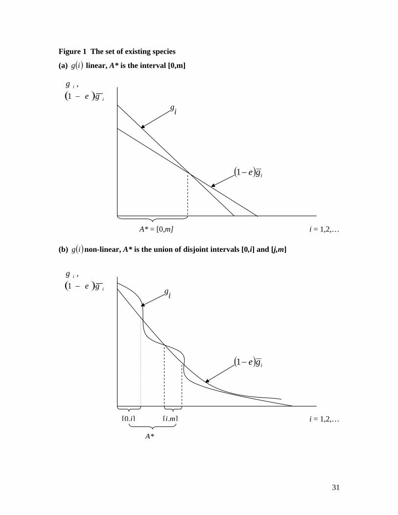
For the intuition behind this consider Figure 1, which graphs ( ) ii geg −1, against i =
1,2,…, assuming continuous species, and shows the set of points, i, for which
( ) ii geg −> 1 . The set, A*, for which this inequality holds is the set of all living species
in the system. Panel (a) illustrates a case where g(i) is linear, and panel (b) a case where
g(i) is non-linear. In panel (a) A* is the interval [0,m]. In panel (b) A* is the union of a
set of disjoint intervals, {[0,i], [j,m]}.
(Figure 1 about here)

10
In the perfectly heterogeneous case (e0 = 1), i.e. where the system is perfectly partitioned,
[12] collapses to a condition that the net growth rate of the competitive dominant species
in each niche is positive. In the perfectly homogeneous case (e0 = 0) the requirement
implies that i
gg
i
j ji
∑ => 1 which, given the ranking of the gi , is satisfied only for species
s1. That is, in the perfectly homogeneous case, competitive exclusion leaves only the first
ranked species in the system. The forgoing is summarized in the following proposition:
Proposition 1: Species existence in the natural system. In a physically closed system in
which the dynamics of the ith of m0 potential species are described by [2], where species
are competitively ranked by their equilibrium abundance, and where φ is evaluated at
[ ]( )m,1φ , a necessary and sufficient condition for the existence of that species in the
steady state is that: ( ) [ ]( ) ( ) 01,1
1 1 >⎟⎟⎟
⎠
⎞
⎜⎜⎜
⎝
⎛
−+
−−>
∑ =
eiem
rdiKeg
i
j jji φ
, where ⎟⎟⎠
⎞⎜⎜⎝
⎛ −=
i
iii r
drKg : .
It is straightforward to show that the number of species that exist is increasing in the
degree of environmental heterogeneity. To see this, consider the case where species are
continuous. Suppose that the set of potential species is [0,m0] and that, as before g(i) is
decreasing in i. We have:
[13] ( ) ( ) ( ) ( ) [ ]( ) ( ) ( )( )0 01, 1ds i r i
s i g i m e s i e Sdt K
ϕ= − − − , i ∈ [0,m0]

11
with
[14] ( )diisS ∫=
being the integral of s(i) over all existing species. It follows that if species i exists in the
steady state, then
[15] ( ) [ ]( ) ( ) ( )0 01, 1g i m e s i e Sϕ= + −
and the least productive of the surviving species – the species with the lowest ‘g’ value –
will solve:
[16] ( ) ( ) ( )01g m e S m= −
where ( )⋅φ is evaluated at the set of existing species [0,m], 0m m≤ , and where
[17] ( ) [ ]( ) ( ) ( )0 0 0
10, 1
m
S m g i dii e e mϕ
⎛ ⎞= ⎜ ⎟⎜ ⎟+ −⎝ ⎠
∫
In the special case where ( )m mϕ = this implies that
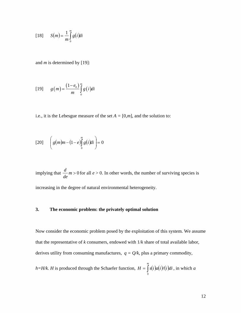
12
[18] ( ) ( )diigm
mSm
∫=0
1
and m is determined by [19]:
[19] ( ) ( ) ( )0
0
1 meg m g i di
m−
= ∫
i.e., it is the Lebesgue measure of the set A = [0,m], and the solution to:
[20] ( ) ( ) ( ) 010
=⎟⎟⎠
⎞⎜⎜⎝
⎛−− ∫ diigemmg
m
implying that 0d mde
> for all e > 0. In other words, the number of surviving species is
increasing in the degree of natural environmental heterogeneity.
3. The economic problem: the privately optimal solution
Now consider the economic problem posed by the exploitation of this system. We assume
that the representative of k consumers, endowed with 1/k share of total available labor,
derives utility from consuming manufactures, q = Q/k, plus a primary commodity,
h=H/k. H is produced through the Schaefer function, ( ) ( ) ( )∫=m
diiiaisH0
, in which a

13
measures the effectiveness of harvesting effort and L is the share of total labor committed
to harvesting S. One unit of Q is produced with 1/k share of labor, and the price of Q is
taken as the numeraire. Since the value of the marginal physical product of labor in
manufacturing is also equal to 1, the wage, w = 1. It follows that Q = 1-L.
The representative consumer solves the following problem: ),( qhuMax subject (a) to a
budget constraint, qkPHk += /1 , where PH is the domestic value of the aggregate
harvested natural resources, and (b) to the dynamics of S. Since both q and h are
‘essential’ it follows that u(0,q) = u(h,0) = 0 and the partial derivatives with respect to h,q
are infinite, i.e. Inada conditions hold. The social problem accordingly takes the
following general form:
[22] ( ){ }∫∞
=
−
0,
t
tL dteQHUMax ρ
subject to the equations of motion for the set of all species, [1], and to the structure of
property rights. Following Brander and Taylor (1997) we assume that the utility function
takes the specific form ( )ββ −1QHU , 0>′U . It then follows that WPH β= and
( )WQ β−= 1 , where P is the domestic price of aggregate harvest, H, and W comprises
both income from labor, Ls, and profits from firms producing H. Note that profits from
firms producing Q are zero by the assumption of constant returns, and wages are set equal
to unity.

14
To begin with, we consider the decision problem in decentralized competitive
equilibrium, assuming that firms internalize all spillovers except for those associated with
the impact of effort on environmental heterogeneity. Each firm exploits a particular
patch and selects the level of harvest effort to maximize steady-state profits from that
patch. To make the biodiversity consequences of economic activity quite transparent, we
consider the special case where future consumption is not discounted, i.e. 0=ρ , and
confine our attention to steady states. In this case the representative firm solves a problem
of the form:
[23] ( ) ( ) ( ) ( ) ( ) ( )iiiaiviPsMax i −=π
subject to [1], noting that v(i) defines the species-specific weight on the domestic price of
aggregate output, P. Hence Pv(i) can be thought of as the domestic price of the ith
harvested species.
The set of species that are actively harvested comprises all those i for which the value of
the marginal physical product of labor is positive at ( ) 0=i , i.e. for which ( ) 0>id
dπ at
( ) 0=i . In the case where the system is perfectly heterogeneous, that is where e = 1, we
can use the steady state formula for ( ) ( )( ) [ ]( )miigis ,1, φ= to show that a sufficient
condition for i to be in the set of harvested, living species is that:
[24] ( ) ( ) ( ) ( )( ) ( ) [ ]( )miridirKiaiPv ,1φ>−
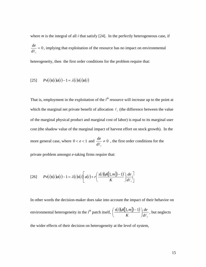
15
where m is the integral of all i that satisfy [24]. In the perfectly heterogeneous case, if
0=id
de , implying that exploitation of the resource has no impact on environmental
heterogeneity, then the first order conditions for the problem require that:
[25] ( ) ( ) ( ) ( ) ( ) ( )iaisiiaisiPv λ=−1
That is, employment in the exploitation of the ith resource will increase up to the point at
which the marginal net private benefit of allocation i (the difference between the value
of the marginal physical product and marginal cost of labor) is equal to its marginal user
cost (the shadow value of the marginal impact of harvest effort on stock growth). In the
more general case, where 10 << e and 0≠id
de , the first order conditions for the
private problem amongst e-taking firms require that:
[26] ( ) ( ) ( ) ( ) ( ) ( ) ( ) [ ]( )( )⎥⎦
⎤⎢⎣
⎡⎟⎠⎞
⎜⎝⎛ −
+=−id
deK
misriaisiiaisiPv 1,11 φλ
In other words the decision-maker does take into account the impact of their behavior on
environmental heterogeneity in the ith patch itself, ( ) [ ]( )( )id
deK
mis⎟⎠⎞
⎜⎝⎛ −1,1φ , but neglects
the wider effects of their decision on heterogeneity at the level of system,
16
( ) ( ) ( ) [ ]( ) ( ) djdde
KSjsmjrjsj
i
m
ij∫ ≠⎟⎠⎞
⎜⎝⎛ −,1φλ . Note that whether the impact on employment
in the resource sector is positive or negative depends on the sign of id
de . Although it is
generally the case that increasing exploitation of ecosystems reduces heterogeneity
through the development of monocultures, this is not always the case.
To obtain the supply curve for aggregate harvest, we evaluate ( ) ( ) ( ) ( ) ( )diisiiaivPHi∫=*
at ( )i* . The market clearing conditions for autarky (assuming that property rights are
well-defined) are, on the demand side:
[27] ( ) ( )P
PLP
PH s πββ
+==
1.*
and on the supply side:
[28] ( ) ( )( )PLLL ss *1* πβ +−=−
For any e in [0,1] competitive equilibrium will determine L* and hence e*, the latter
being the solution to ( )( )eLfe *= . It follows immediately that there may be many
competitive equilibria, but that they may also be welfare-ranked.
To see the effect of exploitation on biodiversity, we define the maximum potential
biomass of the ith of m harvested (discrete) species to be:

17
[29] : i i i ii
i
r d ag Kr
⎛ ⎞− −= ⎜ ⎟
⎝ ⎠
We expect to be able to define a similar cut-off rule for any allocation of harvest effort.
Ranking { }ig , as before, such that 1 2 0mg g g> > > > , we can obtain by similar
reasoning a sufficient condition on ig for the existence of the ith species as a function of
both the biological parameters, ri and di and the level and effectiveness of harvest effort,
iia :
[30] ( ) [ ]( ) ( )1
11, 1
i i ij
ii
d airg e K
m e i eϕ
=
+⎛ ⎞−⎜ ⎟⎜ ⎟> −
− −⎜ ⎟⎜ ⎟⎝ ⎠
∑
In this case, as before, we take the case where A is an interval, i.e. the case shown Figure
1(a). The algorithm used to identify the level of species richness is as follows: for a given
set of environmental conditions, e, set L = 0 and find the set of m species that satisfy
condition [18]. Then increase L until the value of L is found that reduces the number of
species from m to m-1. Continue in this manner until L = 1 at which point ( )( )1ig g e=
is the cut-off (marginal surviving) species. This may be summarized in the following:
Proposition 2: Species existence in an economically exploited system. In an economic
system based on the exploitation of up to m discrete species, ranked according to the

18
maximum potential biomass net of harvest, a necessary and sufficient condition for the
existence of the ith species in the steady state is that
( ) [ ]( ) ( )1
1 01, 1
i i ij
ii
d airg e K
m e i eϕ
=
+⎛ ⎞−⎜ ⎟⎜ ⎟> − >
− −⎜ ⎟⎜ ⎟⎝ ⎠
∑, where : i i i i
ii
r d ag Kr
⎛ ⎞− −= ⎜ ⎟
⎝ ⎠.
From the first order necessary conditions for the solution of the private problem where
firms are e-takers, we can identify the steady state implications for biodiversity of
different levels of environmental heterogeneity in the autarkic system. If the system is
extremely heterogeneous, (e = 1, L > 0), we have the following conditions on si and i :
[31] ⎟⎟⎠
⎞⎜⎜⎝
⎛ −−=
i
iiiii r
adrmKs
[32] ⎟⎟⎠
⎞⎜⎜⎝
⎛−⎟
⎠⎞
⎜⎝⎛ −= i
ii
ii d
Kms
ra
11
from which it is immediate that i is increasing in ri, the natural regeneration rate of the
ith species and decreasing in ai, the technical efficiency of harvest. In the extremely
homogeneous case, (e = 0), [31] and [32] are of the form:
[33] ( )
( )
,
0,
i i i ii m
ii
i m
r d aK g s grs
g s g
⎧ ⎛ ⎞− −=⎪ ⎜ ⎟= ⎨ ⎝ ⎠
⎪ ≠⎩

19
[36] ( )
( )
1 1 ,
0,
i i i mii
i m
Sr d g s ga K
g s g
⎧ ⎛ ⎞⎛ ⎞− − =⎪ ⎜ ⎟⎜ ⎟= ⎝ ⎠⎨ ⎝ ⎠⎪ ≠⎩
If the ith species has the highest ‘g’ value, or net regeneration potential, it will be the
competitive dominant species. If not it will be driven extinct. Similarly, the labor
committed to harvest the ith species will be equal to L if that species has the highest ‘g’
value, and will be zero otherwise.
Now consider the case where there is some environmental heterogeneity, and therefore
some biodiversity, i.e. where 0 < e < 1. We have that:
[35] ( )⎟⎟⎠
⎞⎜⎜⎝
⎛ −−
−=
KSe
rdr
mKs
i
iii
1
As the degree of environmental heterogeneity rises from the point at which the ith species
is able to coexist with other species, the steady state stock of that species first increases
and then declines. Moreover, if the system is subject to exploitation, L > 0, then the
steady state share of the labor force committed to harvest the ith species is:
[36] ( )
⎟⎟⎠
⎞⎜⎜⎝
⎛−⎟⎟
⎠
⎞⎜⎜⎝
⎛⎟⎠⎞
⎜⎝⎛ −+
−= ii
ii
i dK
Seemsr
a1
11
20
As before, it is immediate that i is increasing in ri, the natural regeneration rate of the ith
species and decreasing in ai, the technical efficiency of harvest. i is either decreasing or
increasing in e, as K
Semsi − is positive or negative. This is summarized in proposition 3
below:
Proposition 3: The effect of environmental heterogeneity in an economically exploited
system. If the system is extremely homogeneous (e = 0), the steady state stock of the sole
surviving species will converge to the maximum potential biomass of that species net of
harvest. All other species will be driven extinct. The share of the labor force committed
to harvest that species will be equal to L. If the system is extremely heterogeneous (e =
1), the steady state stock of the ith species will converge to the maximum potential
biomass of that species in the patch within which it is the competitive dominant species.
The share of the labor force committed to harvest the ith species will be increasing in the
natural regeneration rate rate of the ith species and decreasing in the technical efficiency
of harvest. For intermediate levels of heterogeneity, (0 < e < 1), the steady stock of
species that are competitive dominants in existing patches converge to their maximum
potential biomass net of ‘harvest’, and otherwise will fall to zero.
5. The economic problem: the socially optimal solution
The social decision-problem reflects the fact that while e depends on harvest effort by
each firm, it also affects environmental heterogeneity in the system as a whole, and

21
therefore the number of surviving species. Yet the firm may have no incentive to take this
into account. For a given value of e in [0,1] we define the harvest function:
[37] ( ) ∫=i iiii disavMaxeLh :;
in which ( ) 0,0 =eh for e ∈ [0,1]. If property rights are such that the representative firm
takes e as given, they solve the problem:
[38] ( ){ }LeLPhMaxL −; .
subject to Li i =∑ and [1]. The equilibrium associated with this structure of property
rights is defined as {L*,H*,P*(H),e*} such that
[39] ( ) ( ){ }QHUQH ,maxarg**, =
subject to
[40] ( )*1* HQHP π+=+
and L* is given by,
[41] ( ){ }LeLhPL −= *;*maxarg* .

22
Furthermore, the “rational point expectations” condition e* = e(L*) holds. If e(L) = e(0)
is a constant function, the social welfare optimum
[42] ( )( )LLhUL −= 1,0;maxarg*
is the same as L* in [41]. In general, a first order necessary condition for maximizing
social welfare with respect to L is:
[43] ( ) 0=−+ QLeLH UehhU .
In the equilibrium defined by [39] – [41], the term Leeh is absent: i.e. the representative
firm ignores its effect on heterogeneity. Note that the equilibrium defined by [39] – [41]
assumes full property rights to the set of natural resources, but not to the heterogeneity
and hence species richness of the general system.
Now consider the social problem confronting the resource extraction industry. The social
equivalent of the problem specified by [23] is
[44] ( )∫= −=m
i iiiiiSL diavPsMax0
π
subject to the steady state value of [1]. The first order necessary conditions for the
maximization of social profit include the requirement that:

23
[45] [ ]( )
⎥⎦
⎤⎢⎣
⎡⎟⎠⎞
⎜⎝⎛ −
+=−i
iiiiiiii d
deK
SsmrasasPv
,11
φλ , i = 1,2,…,m.
Note that by comparison with [26] this requires the ith firm to take account of the impact
that its effect on environmental heterogeneity has on all others in the industry, measured
by: [ ]( )
djdde
KSsm
rsi
m
ij
jjjj∫ ≠ ⎟⎟
⎠
⎞⎜⎜⎝
⎛ −,1φλ .
Proposition 4. If property rights to natural resources are defined, but exclude rights to
the heterogeneity of the system, then the competitive equilibrium will generate external
costs associated suboptimal levels of heterogeneity, defined by 0>i
ehU eH . For the
social profit maximization problem, the heterogeneity externality of the allocation of
( )i* is defined by: [ ]( )
djdde
KSsm
rsi
m
ij
jjjj∫ ≠ ⎟⎟
⎠
⎞⎜⎜⎝
⎛ −,1φλ .
To see the implications for biodiversity we suppose, without loss of generality, that there
are multiple species, i.e. e > 0, but that only one is economically valuable. We denote the
single valuable species j ∈ {1,2,…, m}and normalize its value. We then have
( ) ( ) jiiPvjPv ≠== ,0,1 . Consider again the problem defined by equations [44] and [1].
The first order conditions for the maximization of social profit for the unvalued species i
require that:

24
[46] [ ]( )
jidde
KSsm
rasi
iiiii ≠⎥
⎦
⎤⎢⎣
⎡⎟⎠⎞
⎜⎝⎛ −
+=− ,,1
1φ
λ
implying that the optimal ‘harvest’ of i, ( ) 0* ≥ih , satisfies:
[45] [ ]( )
jidde
KSsm
rshii
iiiii ≠⎥
⎦
⎤⎢⎣
⎡−⎟
⎠⎞
⎜⎝⎛ −
−= ,1,1*
λφ
.
Consider the conditions in which this term will be positive. From [1] the abundance of
the valued species is impacted by the existence of all other species, regardless of whether
it is the competitive dominant. Hence λi < 0 for all ji ≠ , and there exists an incentive to
‘harvest’ unvalued species. The two polar cases are where j = 1 (the valued species is the
most abundant) and j = m (the valued species is the least abundant). In both cases, the
abundance of the valued species is affected by the existence of competitor species, but
this effect is more significant in the second case. That is, the incentive to simplify the
system by reducing the abundance of unvalued species is stronger the less abundant (the
less competitive) is the valued species relative to other species.
Whether unvalued species are in fact ‘harvested’ depends on the relative strength of the
two terms on the RHS of [45]. If 0=idde , implying that harvest effort has no impact
on environmental heterogeneity at the margin, then 0<iλ is a sufficient condition for
0* >ih . However, if 0≠idde then whether the ith unvalued species is ‘harvested’
depends on the sign of idde and its relative abundance. If 0<idde , implying that
25
harvest effort homogenizes the system, then the optimal level of ‘harvest’ of the ith
unvalued species will be higher if that species has greater than average abundance, and
will be lower if it has less than average abundance. If, 0>idde implying that harvest
effort heterogenizes the system, then the optimal level of ‘harvest’ of the ith unvalued
species will be decreased if that species has greater than average abundance, and will be
increased if it has less than average abundance. In both cases, ‘harvest’ of the ith unvalued
species will fall to zero if [ ]( )
ii
iii d
deK
Ssmrs
λφ 1,1
≤⎟⎠⎞
⎜⎝⎛ −
.
The implications of this for environmental heterogeneity and biodiversity are direct.
Since the presence of unvalued competitor species imposes a social cost in the form of
the reduced abundance of valuable species, there is a positive incentive to reduce the
abundance of those competitors. Whether this leads to positive rates of harvest depends
on the impact of effort on heterogeneity. We summarize this in the following proposition:
Proposition 4. Homogenization and the harvest of unvalued species. If only some species
are positively valued, then since the abundance of those species is reduced by the
existence of unvalued competitors the shadow value of those species will be negative, λi
< 0 for all ji ≠ . This implies a positive incentive to reduce their abundance. If
0<idde , optimal level of ‘harvest’ of the ith unvalued species will be increased if that
species has greater than average abundance, and will be reduced if it has less than
average abundance. If 0>idde , then the optimal level of ‘harvest’ of the ith unvalued

26
species will be decreased if that species has greater than average abundance, and will be
increased if it has less than average abundance.
4. Discussion
The problem addressed in this paper is the economic causes and consequences of
biodiversity change across the whole landscape. While we accept that the loss of refugia
through, for example, the conversion of forests for agriculture is an important driver of
biodiversity loss, it is not the whole story. In this paper we attempt to model a more
general process. This is a process with two main strands. One is the adoption of land
uses that affect the niche structure of the ecosystem. The other is the direct ‘harvest’ of
species, either to exploit the properties of desirable species or to control undesirable
competitor species (‘weeds’). Both strands of the process involve market failure.
While we specify the general form of the growth functions for all potential species in the
system to accommodate the role of competitive exclusion in determining species richness
in environmentally heterogeneous landscapes, we do not specify the form of the function
e(L). How anthropogenic exploitation affects environmental heterogeneity is an
empirical question. Although we expect intensive high-input agriculture to lead to
homogeneous species-poor landscapes, the relationship between effort and environmental
heterogeneity is not necessarily monotonic. At relatively low levels of both heterogeneity
and effort it is possible that environmental heterogeneity is increasing in effort. We show
that if exploitation of the environment leads to its homogenization, and so to a loss of

27
biodiversity, the socially optimal level of effort committed to the harvest of the ith species
will be lower than if exploitation increases environmental heterogeneity. Moreover,
different species may be treated in different ways in the same system. The species
populating home gardens, for example, are exploited in fundamentally different ways
from the species exploited in large scale commercial agriculture, and the environmental
consequences of both activities are quite different.
The impact of declining environmental heterogeneity discussed in this paper includes the
effect of declining habitat noted in a number of studies (e.g. Polasky, Costello and
McAusland, 2004; Barbier and Shultze, 1997). In cases where increasing effort clearly
decreases environmental heterogeneity, the results in this paper are similar to those
identified in such studies. However, whereas these studies associate increasing levels of
effort with declining habitat, and therefore identify a monotonic negative relation
between effort and biodiversity, we allow the effect of effort on biodiversity to be either
positive or negative. Activities that make the environment more patchy increase the level
of species diversity, activities that make the environment more homogeneous have the
opposite effect. We have not considered a second important impact of the loss of
biodiversity associated with homogenization: the effect on the resilience of the general
system and its capacity to maintain productivity over a range of environmental conditions
(Loreau et al, 2003; Kinzig et al, 2006). Since our concern is to model biodiversity loss
itself, this is beyond the scope of the paper, but it is an important dimension of the value
of biodiversity externalities.

28
Once again, the distinction between the case in which decision-makers are free to ignore
the social cost of their access to natural resources and the socially optimal case are
transparent. In the general case, where decision-makers ignore the shadow value of
exploited species and the impact of private land use decisions on environmental
heterogeneity they will both overexploit species and generate a landscape that is less
environmentally heterogeneous than is socially optimal. Once the source and magnitude
of the externality has been identified, standard corrective instruments may be applied.
The aim of the modeling exercise reported here is to help understanding of biodiversity
externalities that include not just the contraction of wild refugia and overharvesting, both
of which have been addressed in the literature, but also the impacts of changes in
environmental heterogeneity. Since being ‘like one’s neighbor’ increases the risk of
extinction of species other than the competitive dominants, it involves an externality that
may be amongst the most important inadvertent drivers of biodiversity loss.

29
References
Barbier E.B. 2007. Valuing ecosystem services as productive inputs. Economic Policy 22
(49): 177–229.
Barbier E. and C. Schulz, 1997. Wildlife, biodiversity and trade, Environ. Devel. Econ. 2
(2): 145–172.
Brander J.A. and M.S.Taylor 1997. International trade and open-access renewable
resources: the small open economy case, Canadian Jnl. Econ. 30(3): 526-552.
Brock W.A. and A. Xepapadeas, 2004. Optimal management when species compete for
limited resources, J. Environ. Econ. Manage. 44(2): 189–220.
Daily G.C; S. Alexander, P.R. Ehrlich, L. Goulder, J. Lubchenco, P.A. Matson, H.A.
Mooney, S. Postel, S.H. Schneider, D. Tilman, G.M. Woodwell, 1997. Ecosystem
Services: Benefits Supplied to Human Societies by Natural Ecosystems Issues in
Ecology 1(2):1-18.
Hooper D. U., Chapin III , F. S., Ewel, J. J., Hector, A., Inchausti, P., Lavorel, S.,
Lawton, J. H., Lodge, D. M., Loreau, M., Naeem, S., Schmid, B., Setälä, H.,
Symstad, A. J., Vandermeer, J., and Wardle, D. A. 2005. Effects of biodiversity
on ecosystem functioning: a consensus of current knowledge. Ecological
Monographs 75 (1): 3-35.
Kinzig, A.P., S.A. Levin, J. Dushoff, and S. Pacala. 1999. Limiting similarity, species
packing, and system stability for hierarchical competition-colonization models.
The American Naturalist 153(4):371-383.
Kinzig, A.P., P. Ryan, M. Etienne, T. Elmqvist, H. Allison, and B.H. Walker. 2006.
Resilience and regime shifts: Assessing cascading effects. Ecology and Society
11(1): article 13 [online]
Loreau, M., N.Mouquet and A.Gonzalez. 2003. Biodiversity as spatial insurance in
heterogeneous landscapes. PNAS 22: 12765-12770.
MacArthur R.H. and E.O. Wilson. 1967. The Theory of Island Biogeography, Princeton
N.J., Princeton University Press.
Millennium Ecosystem Assessment (MA) 2005. Ecosystems and Human Well-Being:
Synthesis. Island press, Washington D.C.

30
Naeem, S. and J. P. Wright. 2003. Disentangling biodiversity effects on ecosystem
functioning: Deriving solutions to a seemingly insurmountable problem. Ecology
Letters 6: 567-579.
Norberg J., D.P. Swaney, J. Dushoff, J. Lin, R. Casagrandi and S.A. Levin 2001.
Phenotypic diversity and ecosystem functioning in changing environmentas: a
theoretical framework, Proceedings of the National Academy of Sciences 98(20):
11376-11381.
Perrings, C. and Gadgil, M. 2003. Conserving biodiversity: reconciling local and global
public benefits. In I. Kaul, P. Conceicao, K. le Goulven, and R.L. Mendoza R.L,
eds. Providing global public goods: managing globalization, pp. 532-555. Oxford
University Press, Oxford.
Polasky S., C. Costello and C. McAusland. 2004. On trade, land- use and biodiversity.
Journal of Environmental Economics and Management 48: 911-925.
Wilcove D. S., D. Rothstein, J. Dubow, A. Phillips, and E. Losos 1998. Quantifying
threats to imperilled species in the United States, Bioscience 48: 607-15.
31
Figure 1 The set of existing species
(a) ( )ig linear, A* is the interval [0,m]
(b) ( )ig non-linear, A* is the union of disjoint intervals [0,i] and [j,m]
ig
( ) ige−1
( ) i
i
geg
−1,
i = 1,2,… A* = [0,m]
ig
( ) ige−1
( ) i
i
geg
−1,
i = 1,2,…
A*
[0,i] [j,m]

32
Top Related