


Languages
Pages
Legal


Institute for Law and Justice 1018 Duke Street Alexandria, Virginia Phone: 703-684-5300 Fax: 703-739-5533
E-Mail: [email protected]
Modeling the Dynamics of Street Robberies
#2005-IJ-CX-0015
November 21, 2008
Prepared by
Elizabeth Groff
Temple University
Project Director
Tom McEwen
Institute for Law and Justice
Prepared for
Office of Justice Programs
National Institute of Justice
Modeling the Dynamics of Street Robberies
Abstract
Achieving a better understanding of the crime event in its context remains an important
research area in criminology that has major implications for making better policy and developing
effective crime prevention strategies. However, progress in this area has been handicapped by a lack of
micro-level data and modeling tools that can capture the dynamic interactions of individuals and the
context in which they occur. This research creates a conceptual model of street robberies that is based
on extant theory and empirical research. Four distinct versions of that conceptual model are
implemented using agent-based modeling software (ABMS). All of these versions incorporate core
elements of routine activity theory—a motivated offender, suitable target, and a lack of capable
guardians. From a research standpoint, this enables specific components of routine activity theory to
be explored within a controlled environment. Specifically, the core premise that changes in the social
structure have increased crime rates will be examined by varying the time spent away from home over
five different temporal experiments. While the original concept of social changes in routine activities
did not explicitly consider spatial aspects, this research draws from the geographic literature on activity
spaces and offender travel behavior. Inclusion of spatial aspects is accomplished by defining two
different types of agent movement—directed and random on two different landscapes – uniform grid
and street network. The focus of this study is on operationalizing theory to study the dynamic
interactions between individuals from which aggregate crime rates and crime patterns emerge.
Research conducted using simulation offers a cost-effective supplement to field research. When used in concert, the two methods focus investments in research by identifying strategies that simulation indicates are promising for further research via field experiments. Research conducted with simulation software offers the ability to examine a variety of policy questions related to crime prevention, policing strategies, and the best response to terrorist incidents. In the area of crime prevention, expensive policies suggested by Crime Prevention Through Environmental Design (CPTED) literature could be tested before investments in physical changes are made. Exploration of the components of the decision to offend (victim selection, guardianship, site characteristics, etc.) will suggest concrete policy direction to prevent crime. Different policing strategies can be tested (e.g., hot spots policing) to examine the rate and size of the resulting diffusion. Finally, simulation can be used to model the reactions of people during catastrophic events. The model developed here provides the foundation for additional, more richly specified models to be developed.

Table of Contents
Introduction .................................................................................................................................... 1
Theoretical Background .................................................................................................................. 5
Routine Activity Theory ............................................................................................................ 5
The Role of Urban Form, Place Characteristics, and Human Activity ....................................... 7
Offender Behavior................................................................................................................... 10
Challenges Encountered by Previous Research ...................................................................... 11
A Brief Introduction to Simulation Modeling ............................................................................... 16
Conceptual Model ......................................................................................................................... 19
Methodology ................................................................................................................................. 21
Agent Analyst- GIS/ABM Integration ...................................................................................... 22
Input Data ......................................................................................................................... 23
Model Parameters .................................................................................................................. 25
Experimentation – Systematic Manipulation of Society through Model Versions ................ 28
Implementation Details ................................................................................................................ 35
Agent Structure and Characteristics ................................................................................. 35
Agent Behavior .................................................................................................................. 38
Model Behavior ................................................................................................................. 42
Landscape Structure ......................................................................................................... 42
Creating Activity Spaces for the Civilian Agents in the Model................................................ 43
Challenges to Learning from Models: Calibration and Validation ............................................... 48
Analysis ......................................................................................................................................... 51

Findings ......................................................................................................................................... 54
Descriptive Analysis ................................................................................................................ 55
Spatial Pattern Differences ............................................................................................... 62
Hypotheses ............................................................................................................................. 65
Hypothesis 1: As the average time spent by civilians on activities away from home
increases, the aggregate rate of robbery will increase. ................................................... 65
H2: The temporal and spatio-temporal schedules of civilians while away from home
change the incidence of robbery events. ......................................................................... 70
H3: As the average time spent by civilians on activities away from home increases, the
spatial pattern of robberies will change. .......................................................................... 74
H4: The temporal and spatio-temporal schedules of civilians while away from home
change the spatial pattern of robbery events. ................................................................. 85
Sensitivity Test Results ...................................................................................................... 90
Summary of Findings............................................................................................................... 91
Explanations for the Emergent Patterns................................................................................. 97
Extending the Model ............................................................................................................... 99
Findings from the Enhanced Model Version .................................................................. 105
Implications for Policy and Practice ............................................................................................ 107
Dissemination of Methodology and Findings ............................................................................. 112
References .................................................................................................................................. 114
Appendix 1: Technical Aspects of Activity Spaces and Agent Movement ..................................... 1
Data Structure to Support Agent Movement in the Model ..................................................... 1
Preparation of Data to Support the Implementation of Agent Movement ....................... 1
Random Movement: Identification of Neighboring Nodes ..................................................... 2
Directed Movement: Step 1 - Creating Activity Spaces ........................................................... 4

Associating Street Nodes with Areal Boundaries ............................................................... 5
Compute Actual Distributions and Agent Distributions of Activities ................................. 6
Randomly Allocate Activity Nodes to Agents ..................................................................... 7
Directed Movement: Step 2 - Identification of Path Taken Among Activity Nodes ................ 8
Directed Movement: Step 3 – Creating a Temporal Schedule ................................................ 9
Appendix 2: Street Robbery Model Documentation: Simple Version .......................................... 1
Appendix 3: Street Robbery Model Documentation: Temporal and Activity Space Versions ..... 1
Appendix 4: Java Code for Proportionately Allocating Agent Homes, Jobs and Activities ............ 1
Appendix 5: Visual Basic Code for Finding the Shortest Path and Outputting a List of Nodes
Traveled .......................................................................................................................................... 1
Appendix 6: Street Random and Grid Random Version Code ....................................................... 1
Appendix 7: Temporal Version Code ............................................................................................. 1
Appendix 8: Activity Space Version Code ...................................................................................... 1
Appendix 9: Extended Activity Space Version Code ...................................................................... 1

Modeling the Dynamics of Street Robbery 1
Modeling the Dynamics of Street Robberies
Introduction Achieving a better understanding of the crime event in its context remains an important
research area in criminology that has major implications for making better policy and
developing effective crime prevention strategies. However, progress in this area has been
handicapped by a lack of modeling tools that can capture the dynamic interactions of
individuals and the context in which they occur. Agent-based models offer the ability to do just
that. An agent-based simulation implemented in the framework of a computational laboratory
offers several advantages (Dibble, 2003; Epstein & Axtell, 1996; Gilbert & Terna, 1999). First,
agent-based models allow heterogeneity among individuals that more closely approximates the
variety found in life. Second, the agents and the landscape can be held constant or
systematically varied in order to provide a level of control impossible to attain using traditional
social science methods. Third, the combination of heterogeneous agents and control enables
the researcher to conduct a variety of experiments using different conditions or applying
various prevention scenarios and then to evaluate outcomes for minimal cost compared to
experiments in the real world.
Previous attempts to explain observed crime rates or individual-level victimization have
been based on routine activity theory and relied on a variety of methodologies. Some of the
studies used macro-level data (e.g., city, nation) (Miethe, Stafford, & Long, 1987; Osgood,
Wilson, O'Malley, Bachman, & Johnston, 1996) and others relied on survey data collected from
individuals (i.e., micro-level) (Cohen, Kluegel, & Land, 1981; Kennedy & Forde, 1990; Miethe &

Modeling the Dynamics of Street Robbery 2
McDowall, 1993; Rountree & Land, 1996; R. Sampson, J. & Lauritsen, 1990; R. J. Sampson &
Wooldredge, 1987). Another group of studies combined information about individuals (micro-
level) and the areas in which they lived (macro-level) to represent routine activities within a
social structure (Clarke & Cornish, 1985; Cornish & Clarke, 1986; Walsh, 1986). Although these
studies have contributed to the overall body of knowledge, they have produced inconsistent
empirical support for routine activity theory. These studies suffer from three main
shortcomings: inadequate attention to the spatio-temporal structure of routine activities;
measurement issues; and failure to capture the dynamic interactions of individuals and the
context in which they occur.
This research addresses the issues encountered in earlier studies by designing and implementing an
agent-based model for exploring the contextual aspects of individual crime events and how they
culminate in emerging crime patterns. This initial research focuses on street robbery with a weapon for
three reasons1. The crime of street robbery offers several advantages for this study: 1) it is an
instrumental crime and thus more likely than expressive crimes to involve a rational decision process
(Cohen & Felson, 1979); 2) street robbery is by definition restricted to the street or some other exposed
area rather than in a residence or business and thus involves the public intersection of offender and
target in space and time; 3) police presence is assumed to be more effective against street level crime
then crimes that take place indoors (e.g., domestic violence).
The model is informed by several of the opportunity theories in criminology and two
geographical theories. Opportunity theories include routine activity theory (Clarke & Cornish,

Modeling the Dynamics of Street Robbery 3
1985), rational choice theory (P. Brantingham & P. Brantingham, 1981a; P. J. Brantingham &
Brantingham, 1984) and environmental criminology (Horton & Reynolds, 1971). From
geography we incorporate research on activity spaces (Hägerstrand, 1970, 1973) and time
geography (Cohen & Felson, 1979).
The research is motivated by the need for tools that allow theory strengthening and
exploration of policy alternatives in a cost effective manner. Simulation modeling holds the
promise of facilitating the development of better theories and providing a new way to the
policy implications of research ‘in silica’. Specific to crime prevention, simulation models could
be used to: (1) identify situational characteristics that create the potential for crime to occur;
and (2) test the impact of policy changes on in silica crime rates. The situational elements of
the convergence of offender and victim at a specific place and time can be simulated via agent-
based modeling software. As the initial foray into this area, this study focuses on the
development of a computational laboratory for modeling some simple, dynamic interactions
between individuals from which aggregate crime rates and patterns of crime emerge. Once
this model is built, it can be extended to serve as a laboratory for testing other facets of
criminological theory and police practice at the micro level. In this first set of models, there is
no attempt to incorporate the motivations behind either criminality or guardianship. More
complex issues such as those will be addressed in later studies using the basic framework
developed here. The results of this and subsequent experiments will inform crime prevention
1 The author is grateful to Marcus Felson for pointing out that the model actually represents interactions more similar to those for a street robbery with a weapon. Robberies without a weapon tend to have more than one perpetrator and a model should include those co-offenders.

Modeling the Dynamics of Street Robbery 4
strategies and contribute to the body of knowledge in both environmental criminology and
situational crime prevention.
The goal of this research is to provide additional insight into routine activity theory and
its underlying assumptions. While the research method shows significant promise for assisting
with theory development and for exploring and strengthening existing theory, its utility for
predicting outcomes is still uncertain. Much work remains to be done regarding the calibration
and validation of such models with imperfect empirical data (Axelrod, 2006; Gilbert & Terna,
1999; Gilbert & Troitzsch, 2005). Readers are cautioned that the outcome of the effort was not
designed to provide the ability to predict crime rates. Rather, the knowledge gained is
important to increasing our understanding of the central role of convergence in setting the
stage for street robberies to occur. The research also clearly demonstrates the importance of
the street network and of spatio-temporal constraints on activity spaces in structuring outcome
patterns of street robbery events. These findings highlight important factors that should be
included in empirical studies.
This report begins with the theoretical background for the proposed research including
the challenges that exist in trying to test a micro level theory using macro level data. This is
followed by an introduction to simulation modeling as a methodology that addresses many of
those issues. The next section describes the methodology including the specific hypotheses to
be tested and a detailed specification of the model. The expected results are then discussed.
Analytical techniques that will be employed to test the results are presented. A discussion of
the implications for policy and practice is offered as well as an agenda for further research.

Modeling the Dynamics of Street Robbery 5
Theoretical Background Fortunately, there is rich, theoretical background literature to guide the development of
an agent-based model. Traditionally, criminological theory has focused on the individual and
understanding the root causes of individual criminality. More recently, a number of
criminologists have addressed the specific situation in which the offender makes the decision to
offend. In particular, routine activity theory (P. J. Brantingham & Brantingham, 1991),
environmental criminology (Clarke & Cornish, 1985) and rational choice theory (Cohen &
Felson, 1999) embody this line of research. These more modern theories draw from the
classical school of criminology proposed by Beccaria (1764, translated 1963). Beccaria was the
first to suggest that criminals act in their own self-interest and rationally consider the potential
costs and benefits before committing a crime2. While this view fell out of favor in the 1800s
and most of the 1900s, it was reinvigorated and expanded by the above theorists3.
Routine Activity Theory
Opportunity theories build on the assumption that the decision to offend is an active
one and based on perceived risk versus perceived gain but expand their focus to include the
contextual elements of the crime event. Routine activity theory captured this enlarged focus by
identifying three elements necessary for a crime to occur:(1) a motivated offender, (2) a
2 In addition, Beccaria (Hindelang, Gottfredson, & Garofalo, 1978) believed that punishment would only be effective if it had the following characteristics: certainty, severity (in proportion to the crime), and celerity (administered promptly).
3 Lifestyle theory (Meier, Kennedy, & Sacco, 2001) was also an important theory under the rubric of opportunity theories that is pertinent to micro-level modeling. As is the more recent criminal event perspective (CEP) (Akers, 2000; Cullen & Agnew, 1999; Vold, Bernard, & Snipes, 2002) However, space constraints prohibit a full examination. Three books on the theoretical foundations of criminology offer a more complete overview of opportunity theories (1986).

Modeling the Dynamics of Street Robbery 6
suitable victim, and (3) the absence of capable guardians4. Cohen and Felson (1979) postulate
that simply having a motivated offender, a suitable target, and the lack of a capable guardian at
the same place and time is enough for a crime to occur. However, if even one of the three
elements is missing, a successful crime will not occur. They go on to conjecture that if all three
elements are present, crime may increase even if the proportion of motivated individuals and
the proportion of suitable targets remains the same.
That is, if the proportion of motivated offenders or even suitable targets were to
remain stable in a community, changes in routine activities could nonetheless alter
the likelihood of their convergence in space and time, thereby creating more
opportunities for crimes to occur. Control therefore becomes critical. If control
through routine activities were to decrease, illegal predatory activities could then be
likely to increase … p.258-259.
As is apparent from the quote above, Cohen and Felson (1979) view routine activities
(defined as time spent away from home) as the key dynamic element determining aggregate
crime rates because it affects all three componentslevels of guardianship and the mobility of
both motivated offenders and suitable targets. Changes in routine activities directly impact the
frequency of convergence among these elements that in turn, increase or decrease overall
crime rates. In fact, they go further and suggest that the relationship between the convergence
of the elements and crime rates is not additive but rather multiplicative (1987, p. 913). If the
4 There have been extensions to the theory since the original formulation. In 1987, Felson extended the model to include the importance of place. The concept of guardianship was refined by Felson (1995b) to include the role of intimate handlers and by Eck (Miethe & McDowall, 1993; R. J. Sampson & Wooldredge, 1987) to include the role of place managers. These additions are beyond the scope of the initial models but will represent important enhancements to subsequent models.

Modeling the Dynamics of Street Robbery 7
convergence rate of motivated offenders and suitable targets without capable guardians
increased by some percentage, the resulting crime rate would increase by much more.
Two notions in routine activity theory are of particular interest for this proposal. First,
the idea that crime can increase without increasing the supply of any one of the three elements
simply by changing the amounts of time individuals spend away from home can be explored. In
routine activity theory, changes in social structure drive changes in routine activity. For
example, the movement away from home-centered activity to other locations has both
removed people as guardians of property and increased their personal exposure. Second, the
spatially undefined concept of routine activities as defined by Cohen and Felson (1979) can be
compared to activity spaces that are spatially defined. In Cohen and Felson’s (1979) original
work they conceptualize routine activities in terms of social structure, as occurring either at
home or away from home but the spatial patterns of those activities are never explicitly
addressed. For example, they discuss how home-centered routine activities such as playing
games have been replaced with a variety of activities outside the home (e.g., attending
concerts, working out at the gym, etc.) but do not explore how the spatial patterns inherent in
routine activities might facilitate the convergence of suitable target and motivated offender.
The Role of Urban Form, Place Characteristics, and Human Activity One of the core concepts in routine activity theory involves the necessity of the convergence of
victims and offenders in space and time. The specific ‘where’ and ‘when’ of convergence stems from
the routine behavior patterns of each actor involved. Thus representing the spatio-temporal patterns in
human behavior that facilitate convergence is a critical element to the testing routine activity theory.

Modeling the Dynamics of Street Robbery 8
Individual travel patterns involve a complex space-time balancing act. Scholars have long recognized
that capturing only a single dimension leaves more questions than are answered.
Several significant areas of research can contribute to our understanding of human spatial
behavior. Zipf’s “Principle of Least Effort” (as summarized in Felson 1987) offers a view of human
behavior which states that, in general “people tend to find the shortest route, spend the least time, and
seek the easiest means to accomplish something” (Chorley & Haggett, 1967; Hägerstrand, 1973; Harvey,
1969; Horton & Reynolds, 1971). The spatio-temporal aspects of this simple observation have been
more fully explored and structured by a variety of geographers. In fact, the importance of incorporating
space and time in models of human behavior has long been recognized (Aitken, Cutter, Foote, & Sell,
1989; Gold, 1980; Golledge & Timmermans, 1990; Timmermans & Golledge, 1990; Walmsley & Lewis,
1993).
More specifically, work in the field of behavioral geography provides a well thought-out
foundation for examining the spatio-temporal structure of routine activities in general. Behavioral
geography recognizes the importance of interactions between humans and their environment as the
source of explanation for observed spatial patterns (Hägerstrand, 1970). Within behavioral geography,
time geography (Horton & Reynolds, 1971) and activity space research (Thrift & Pred, 1981) are most
relevant to this undertaking.
The time-geography perspective takes into account the spatio-temporal aspects of human
behavior as situated within the larger social processes (1970; 1975). Hagerstrand (Hägerstrand, 1970)
created this perspective and put forward a conceptual structure for undertaking such studies. In time-
geography, time and space are components of every action and interaction. One cannot be considered
without the other. Individuals travel to various locations along paths. They operate with a known
domain and points at which individuals stop their spatial movement (e.g. work, school, recreation) for a

Modeling the Dynamics of Street Robbery 9
time are referred to as stations. A large part of human interaction occurs at stations. None of these
elements are static, for example, domains and bundles can change as people change jobs or as their
circumstances change (Pred, 1996).
Individual’s travel patterns are influenced by constraints (temporal, economic and spatial) on
their ability to take advantage of opportunities for housing, employment, recreation etc. As a
consequence of including both opportunities and constraints, time-geography offers the potential for
specifying the necessary conditions for all types of human interactions (Pred, 1996). Time-geography
also recognizes the importance of examining both events and nonevents. Focusing on individual
opportunities and constraints as they play out within a particular context is essential to understanding
why events occur sometimes and not others. Another important element of time-geography is the
acknowledgement that examining space-time yields a different and more complete representation of a
situation than the traditional method of studying temporal variation or patterns in space individually
(2006). The joint examination of space-time is critical to improving understanding of human activity.
Ratcliffe (1971) notes the utility of these principles in explaining criminal behavior.
Work done by Horton and Reynold’s (Golledge, 1978; Golledge & Stimson, 1997) on the
concepts of action space and activity space has had considerable influence. Action space includes the
entire set of locations and paths with which an individual is familiar. Activity space, on the other hand, is
more restricted and only includes the places that an individual interacts with in the course of his or her
daily activities. From an activity space viewpoint, home tends to be the dominant node and travel tends
to be concentrated along certain routinely frequented paths. Frequently traveled paths may be
important factors in determining aggregate crime patterns because they bring offenders and victims
together in space and time.
Modeling the Dynamics of Street Robbery 10
Related research examining how individuals acquire spatial knowledge provides similar findings
to activity space research and both are relevant to the current undertaking. The notion of anchorpoints
was developed as part of the body of research on how people learn their way around the urban
environment (Golledge & Stimson, 1997). They found that locations such as home, work and routinely
visited shopping places provide anchorpoints in the knowledge acquisition process. People tend to learn
about the areas between and around anchorpoints first. Over time, a spread effect occurs as people
learn more details about the areas immediately surrounding and along the routes to and from their
anchor points (Cohen & Felson, 1979; Cohen et al., 1981; Felson, 1987; Felson & Clarke, 1998). In this
way, an individual’s knowledge about the urban environment increases incrementally. Logically, those
individual’s with more anchorpoints or with anchorpoints that are more dispersed will have more
extensive knowledge of the urban environment.
Together this collection of research provides a strong basis for conceptualizing routine activity
spaces of individuals as a set of places and the paths between those places. Specifically, the places
consist of a home, a main node (e.g. work, school, etc.), and at least two places that are visited
frequently such as a gym, grocery store, dry cleaner, class etc. The paths among the places are
structured by the street network.
Offender Behavior
As previously mentioned, routine activity theory pays little attention to the source of
the offender’s motivation. In fact, in their own research, Cohen and Felson, (Clarke & Cornish,
1985) assume a supply of motivated offenders and focus on suitable targets and capable
guardians. The complex phenomenon of guardianship is not examined in detail and is
operationalized as presence versus absence. When people are at home, they function as

Modeling the Dynamics of Street Robbery 11
guardians for the property and are personally safer. When they leave, the victimization
potential of both the property (to burglary) and the person (to personal crime) increases.
This research draws upon rational choice perspective to model the decision to offend
(Akers, 2000; Cullen & Agnew, 1999; Felson, 1987; Vold et al., 2002). Rational choice
perspective is based on the economic principle of expected utility where each individual’s
decisions are predicated upon balancing projected benefits against projected costs of activities.
However, Clarke and Cornish (1985) explicitly recognize the importance of situation in
determining the decision to offend. They argue that an individual makes the decision to
commit a particular offense based on the characteristics of the specific situation using bounded
rationality (i.e., the usually imperfect knowledge of the moment as filtered by the particular
cognitive ability of the individual). Clarke and Cornish identify two distinct decision
modelscriminal involvement and commission of a specific crime. This research is only
concerned with the decision to commit a specific crime and assumes the decision to become
involved in the criminal enterprise has already been made.
Challenges Encountered by Previous Research
The crime reduction potential of the routine activity approach is widely recognized
(Cohen, 1981; Messner & Blau, 1987; Miethe, Hughes, & McDowall, 1991). Because this
approach focuses on the situation and not the motivations of the actors, it is easier to generate
concrete implications for both policy and practice. Accordingly, there have been many
attempts over the last 25 years to empirically validate routine activity theory with varying
degrees of success. Some have been conducted using only macro-level data to approximate the
Modeling the Dynamics of Street Robbery 12
construct of routine activities (Miethe et al., 1987; Osgood et al., 1996). Others have relied on
survey data collected from individuals (Cohen et al., 1981; Kennedy & Forde, 1990; Miethe &
McDowall, 1993; Rountree & Land, 1996; R. Sampson, J. & Lauritsen, 1990; R. J. Sampson &
Wooldredge, 1987), and still others have combined micro- and macro-level variables to
represent routine activities within a social structure (Kennedy & Forde, 1990; Miethe &
McDowall, 1993). These studies have found inconsistent support for the theory. In addition,
they suffer from three main shortcomings related to failure to consider the spatio-temporal
structure of routine activities, measurement issues, and inability to represent patterns
emerging from individual-level interactions.
Although the importance of spatio-temporal elements in routine activities is often
acknowledged, the spatial structure and timing of these activities has been widely overlooked.5
Indeed none of these studies attempted to model the dynamic, spatio-temporal interaction of
offenders, victims, and potential guardians at the micro level. In a commendable effort, two
studies attempted to address these issues through the inclusion of gross measures of timing
(e.g., breaking out daytime from nighttime activities) (Cohen et al., 1981; Miethe et al., 1991; R.
J. Sampson & Wooldredge, 1987). However, the spatio-temporal structure of routine activities
is a core component of routine activity theory and deserves more comprehensive
measurement. Since the characterization of routine activities of victims, offenders, and
5 Studies using traditional methods did not explicitly test the geographical and temporal aspects of routine activities at the micro-level. Two studies (Dibble, 2003, 2006; Epstein & Axtell, 1996; Gilbert & Terna, 1999) emphasized how opportunity structure changed across areas but neither measured how the spatial structure of routine activities impacted the observed distribution of crime.

Modeling the Dynamics of Street Robbery 13
guardians is crucial to testing their impact on the spatial structure of observed crime rates, it is
a central piece of this research.
A variety of measurement issues arise when attempting to test routine activity theory
(1993, p. 77). As Bursik and Grasmick note “it has been notoriously difficult to collect reliable
and valid indicators of its central components” (Eck, 1995a). Other measurement issues
include: ecological fallacy; overlapping operationalization of constructs; difficulty with
adequately measuring the construct of routine activities; and a reliance on official data and
victimization surveys that have widely-recognized flaws. When tests are done using macro-
level data, they are susceptible to the ecological fallacy that states that the characteristics of an
area cannot be accurately inferred to individuals. Consequently, macro-level data are
unsuitable for testing a micro-level theory such as routine activity (Miethe et al., 1991; Miethe
et al., 1987). Regardless of the level of analysis, all studies have struggled with measuring the
construct of routine activities as isolated from other constructs being measured. This problem
is closely related to more general issues that have arisen when attempting to clearly link
empirically measured variables to particular constructs (e.g., single person households are
associated with less informal social control and with less guardianship).6 These issues make it
difficult to test the theory because data issues rather than theoretical ones can be used to
dispute contrary evidence (Gove, Hughes, & Geerken, 1985). In addition, the reliance on official
data and victimization surveys, which have widely-recognized flaws, makes conclusions drawn
from studies using those sources suspect (Eck, 1995a).

Modeling the Dynamics of Street Robbery 14
Finally, all of the previous tests reviewed here suffer from a failure to model the
complex and dynamic interactions of individuals that produce observed crime patterns.
Routine activity theory is essentially a micro-level theory with macro-level implications; it
characterizes crime patterns as resulting from the decisions of individuals made in the context
of a particular situation (Liu, Wang, Eck, & Liang, 2005). The methods used in previous studies
were simply not able to accommodate the complex, non-linear nature of individual-level
interactions and the manner in which crime rates emerge from those interactions (Dibble,
2003; Epstein & Axtell, 1996; Gilbert & Terna, 1999). Testing routine activity theory requires a
method that is capable of modeling the dynamic, spatio-temporal interaction of offenders,
victims, and potential guardians at the micro level. The combination of agent-based models
and GIS offers just such a model.
This research advocates a slightly different approach to exploring the foundations of
routine activity theory: computational laboratories using agent-based models. As mentioned
earlier, computational laboratories enable the researcher to study dynamic processes over time
under controlled, repeatable conditions (Boruch, 1997; Sherman & Weisburd, 1995). In order
to better understand the role of routine activities in the convergence in space and time of a
motivated offender, suitable target, and lack of a capable guardian, we need to be able to
model how the individual decisions of heterogeneous agents translate into aggregate rates of
crime. Thus, computational laboratories enable the first direct exploration of Cohen and
Felson’s core assertion that changes in routine activities cause changes in crime rates. As
6 For a thorough review of these types of issues please consult Cohen (1981) and Miethe, Hughes et

Modeling the Dynamics of Street Robbery 15
previously noted, earlier research was limited to using indirect measures of the core elements.
However, computational laboratories allow the researcher to directly manipulate the level of
routine activities. Computational laboratories also allow the researcher to vary one aspect of
the study while holding all others constant, giving a level of control usually not obtainable in
research with human subjects. In this case, each experiment holds the number of motivated
offenders and suitable targets constant, only the amount of time spent at home will vary for
the agents in the model. Finally, computational laboratories make possible the use of agents
with characteristics that are randomly assigned eliminating the possibility of systematic bias.
An advantage of randomized experimental designs is they minimize the potential for systematic
bias between groups (Gilbert & Terna, 1999; Ostrom, 1988), a trait shared by well-designed
agent-based models.
This research specifically examines two aspects of routine activity theory. One is the
core assertion that changes in the structure of routine activities increase crime. This will be
explored using five different levels of time spent away from home. The other aspect that is
examined concerns the impact of geography on routine activity theory. Specifically, does
change in the spatial structure of routine activities cause changes in crime rates or crime
patterns? Three types of agent travel are used across two different landscapes (i.e., uniform
grid and the street network) as the base for a total of twenty experiments examining the impact
of spatial behavior (each type of travel is run across all five levels of time spent away from
home and on the two landscapes).
al. (1991).

Modeling the Dynamics of Street Robbery 16
A Brief Introduction to Simulation Modeling Simulation modeling offers an alternative method for capturing the dynamic interactions
among individuals taking place at the micro level and their relationship to macro level patterns.
Some researchers view simulation as a third way of conducting social science research in
addition to the more traditional verbal and mathematical/statistical representation of theories
(Dowling, 1999; Eck, 2005; Eck & Liu, 2008a; O'Sullivan, 2004). In this tradition, simulation
allows for the exploration and elaboration of theory (Gilbert & Terna, 1999). Like other
modeling approaches, simulation modeling involves the creation of a simplified representation
of a social phenomenon (Dibble, 2003; Epstein & Axtell, 1996; Gilbert & Terna, 1999). The most
familiar type of model is a statistical one (e.g., a regression model) in which input data are ‘run’
via a statistical program and values are output that describe the relationships among the input
data. In contrast, simulation models are themselves computer programs that incorporate the
critical aspects of the social phenomenon being modeled. The program is run and the output
data are analyzed, often via standard statistical techniques. Simulation modeling has two main
advantages over statistical models. It allows heterogeneity among individuals that more closely
approximates the variety found in everyday life and is able to accommodate the non-linear
relationships present in dynamic and complex interactions (Epstein & Axtell, 1996; Gilbert &
Troitzsch, 1999).
Agent-based modeling (ABM) is one type of simulation. ABM employs a bottom-up
approach; agents are imbued with unique characteristics and general behavioral rules and
macro-level patterns emerge from their interactions (O'Sullivan & Haklay, 2000, p. 13). An
agent “can be thought of as an autonomous, goal-directed software entity” (Brown, Riolo,

Modeling the Dynamics of Street Robbery 17
Robinson, North, & Rand, 2005; O'Sullivan & Haklay, 2000). Agents most often represent
people but can also correspond to organizations, neighborhoods, governments etc. The
characteristics of agents can be randomly assigned so that specific societal averages are
produced and the possibility of systematic bias is all but eliminated. Individual agents in the
model interact with each other based on a set of decision rules. Their characteristics are
dynamically changed as a result of those interactions. Traditionally, agents interact in an
artificial world, although the value of leveraging GIS data to provide a ‘real’ landscape is gaining
recognition since artificial landscapes do not take into account the impact of the environment
on agent behavior (Dibble, 2003, 2006; Epstein & Axtell, 1996; Gilbert & Terna, 1999; Macy &
Willer, 2002).
Additional scientific rigor is achieved when simulation models are implemented within a
computational laboratory framework (2001).7 Computational laboratories enable experiments
to be conducted and replicated. Aspects of the agents, society, and the landscape can be held
constant or systematically varied in order to provide a level of control impossible to attain using
traditional social science methods. These characteristics of computational laboratories
facilitate the creation of a variety of simulated experiments, featuring different conditions or
applying various prevention scenarios, which are then evaluated. An added advantage is that
compared to empirical research, simulations have minimal cost.
7 The term computational laboratory refers to the software tools to create and evaluate models through systematic experimentation and descriptive analysis of output data (Axelrod, 2006).

Modeling the Dynamics of Street Robbery 18
Recently, a small body of research has emerged that makes use of simulation models to
explore crime-related issues. Work by Epstein, Steinbruner and Parker (2001) on civil violence
and Wilhite (P. L. Brantingham & Brantingham, 2004; P. L. Brantingham & Groff, 2004) on
protection and social order provide interesting approaches to modeling how the interactions of
individual agents are related to emerging patterns of violence or protection. Within
criminology, work has begun on conceptualizing the application of simulation in environmental
criminology (Eck, 2005) and explaining crime patterns (Birks, Donkin, & Wellsmith, 2008). ABM
is being applied to study both physical (Gunderson & Brown, 2003) and cyber crime (Wang,
2005; Wang, Liu, & Eck, 2004), and some researchers are combining ABM with other
technologies. One example implements a general model of crime on a GIS-based raster grid
(Liu et al., 2005). Another study, based on routine activity theory, employs cellular automata to
study street robbery in one neighborhood (Eck & Liu, 2004). Rather than offering competing
paradigms, these approaches represent a healthy variety of complementary approaches (Eck &
Liu, 2008b). Simulation in criminology is the subject of a recent book (E. R. Groff & Mazzerole,
2008) and a special issue of the Journal of Experimental Criminology (Brown et al., 2005).
The approach taken in this research emphasizes exploration of the mechanisms involved in
street robbery not the prediction of the rate or pattern of street robbery. In doing so, the
research extends previous efforts in several ways. First, the steps involved in building and
applying a simulation model are thoroughly explained to aid in replication. Second, a set of
experiments is conducted to provide the first direct test, albeit in an artificial society, of Cohen
and Felson’s core assertion that shifts in routine activities away from home, increases crime
rates. Each experiment holds the number of motivated offenders and suitable targets constant,

Modeling the Dynamics of Street Robbery 19
only the amount of time spent at home varies for the agents in the model. Third, software
integrating ABM and GIS is used to explore how agent travel on a real street network impacts
the frequency of convergence of the elements necessary for a crime to occur. GIS software
excels at managing data about space and ABM is superior at keeping track of time; together
they allow exploration of space-time relationships. Finally, the new approach allows
examination of how the convergence of heterogeneous agents translates into aggregate rates
of street robbery.
Conceptual Model The preceding review of research identifies the basic elements represented in the
conceptual model (see boxes in Figure 1). The conceptual model identifies two classes of
people, civilians and police. Civilians have activity spaces and can take on different roles (i.e.,
offender, victim, or guardian) depending on the particular situation. Police exist only as agents
of formal guardianship. Civilians with criminal propensity can potentially take on any one of
three roles, offender, victim or guardian. Civilians without criminal propensity can be either
victims or guardians. In addition to criminal propensity, each civilian in the model has a unique
set of characteristics that include wealth and employment status.
Two other spatial elements are important to convergence of people in a model of street
robbery. One is the activity spaces of the people and the other is the network of streets
available for travel. The size and form of activity spaces is influenced by the distribution of
residential housing, jobs, schools, retail, and services. Each civilian has a unique activity space

Modeling the Dynamics of Street Robbery 20
reflecting the places they visit. 8 Once convergence occurs, factors such as guardianship and
suitability of target are considered by the offender when making the decision whether or not to
commit a robbery.
8 This simplistic view of human spatial behavior does not consider the role of trip purpose in determining timing or mode of travel. Mode of travel is an important determinant of exposure (i.e. risk of victimization) and should be incorporated in future models.

Modeling the Dynamics of Street Robbery 21
Figure 1: Conceptual Model of Crime
Methodology This section describes the methodology for ‘situating’ simulation models including software,
data, movement and activity space formulation that is used in the research. Recent
developments in technology and increased data availability at the micro-level support this
approach to modeling individual-level phenomena. The move to object-oriented architecture
provides the technical foundation for the integration of GIS and ABM. Specifics about the

Modeling the Dynamics of Street Robbery 22
software package used to implement the methodology are related. In addition, the data used
to inform agent movement and the activity spaces of the agents is described. Next, the
implementation of random and directed movement of agents in the model is explained. The
details of how agent activity spaces are constructed so they reflect the actual distributions of
homes, jobs and opportunities for retail, recreation, and services are provided. Finally, the
design of the experiments used to test routine activity theory is discussed.
Agent Analyst- GIS/ABM Integration
The method uses a new software package, Agent Analyst, which integrates GIS and ABM to
provide a platform for the dynamic modeling of individuals across space and time.9 This
package follows the middleware approach in which the temporal relationships are handled by
the ABM software and the topological relationships are managed by the GIS (Dibble, 2003;
Epstein & Axtell, 1996; Gilbert & Terna, 1999). Agent Analyst combines two of the most
popular packages for ABM and GIS, the Recursive Porous Agent Simulation Toolkit (Repast) and
ArcGIS. To make the software easier to use, Agent Analyst is built using the rapid development
version of Repast called Repast for Python Scripting (RepastPy) which has a graphical user
interface that automates much of the programming to create the framework of a model. Agent
Analyst is designed to be added into ArcGIS as a toolbox. Once the toolbox is added in ArcGIS,
individual models can access shapefiles allowing: 1) individual agents to become spatially aware
and 2) the visualization of agent movement and decision outcomes (e.g. locations of crimes).
9 Agent Analyst under development as a partnership between ESRI and Argonne National Laboratories; they are the parent companies of ArcGIS and Repast respectively. Agent Analyst is free but currently available by request only. The website for Repast is http://repast.sourceforge.net/.
Modeling the Dynamics of Street Robbery 23
The integration of GIS and ABM enables the exploration of how individual decisions by
heterogeneous agents translate into aggregate rates of street robbery. ABM permits the
researcher to: 1) collect data about the characteristics of each individual present during an
interaction; 2) randomly assign characteristics to agents greatly reducing the possibility of
systematic bias; 3) allow agents to make independent decisions within behavioral guidelines;
and 4) systematically vary one attribute while holding all others constant to undertake
controlled, repeatable experiments (U.S. Census Bureau, 2000). GIS makes it possible to take
into account how the characteristics of the real environment (i.e. street network, distribution of
homes, jobs and activities) impact the activity spaces of agents. In addition, it provides the
ability explore the role of routine activities in facilitating the space-time convergence of a
motivated offender and a suitable target, without a capable guardian present.
Because of its roots in RepastPy, there are several challenges to developing a model using
the beta version of Agent Analyst used in this research. First, the version only supports
interaction with shapefiles, not geodatabases or network data sets. Thus, dynamic routing
along a street network is unavailable for this version. The debugging tools are extremely
limited. Only error messages are provided. Finally, would-be modelers must become familiar
with a unique subset of Python syntax and any Java classes that are needed. However, Python
is a much less demanding language than Java which speeds programming.
Input Data

Modeling the Dynamics of Street Robbery 24
The initial implementation of the model is situated in Seattle, Washington which provides
the data for the street model landscape and the agent activity spaces.10 In addition to input
data, a number of parameters are set in the model. Finally, a variety of outcome data
describing individual-, place- and societal-level characteristics are collected during the ABM
model runs.
Four datasets describing conditions in Seattle are used to inform the activity spaces of
agents in the model: 1) total population; 2) total employment; 3) total potential activities and 4)
streets11. Block group level population figures are used to describe the distribution of
residences across Seattle (Axelrod, 2006). Employment data are used to describe the number
of employees per zip code area.12 Total potential activity locations are quantified through the
use of retail and service establishments (e.g. grocery stores, convenience stores, dry cleaners,
10 A uniform grid landscape is also used as a ‘null’ model. The grid landscape is constructed so that the number of intersections in the grid is as close as possible to the number in the street network. See the section on creating a uniform landscape for more details.
11 The three data sets are at different spatial resolutions. Data on population is at the census block group level. Data on activities arrived as address points and is aggregated to the block group level of analysis. Data describing total employment is only available for zip codes. Since zip codes are much larger than block groups, the data on job locations is not as precise as that for block groups. This is a minor limitation since the goal is to distribute job locations of agents proportionately and not exactly. No attempt is made to model commuting patterns coming into or going out of Seattle.
12 Employment data are from the 2002 County Business Patterns dataset. Employment data are not available by block group, only by zip code. Since there far fewer zip codes (n=56) than block groups (n=570) in Seattle, the employment data is less precise than the block group data. Specifically, the areal units to which jobs are aggregated are much larger than block groups and thus the potential for allocating agents in a way that is not reflected by the actual distribution of employment is higher. This is a minor limitation since the goal is to distribute job locations of agents proportionately, not exactly.

Modeling the Dynamics of Street Robbery 25
gyms etc.).13 The final input data set the street network which is derived from the King County
Street Network Database (SND) file and is used to structure the agent’s movements.
In addition to the input data describing Seattle, a number of parameters are set prior to the
model run. The twelve parameters in the implementation model and the rationale for their
initial settings are described in detail in the next section. One type of parameter used is
random number seeds. Using explicit random number seeds provides the ability to replicate
the model behavior over subsequent runs and is essential to using simulation as a laboratory
for experimentation (Liu et al., 2005).
The outcome data from the simulation are collected for individual civilians, street
nodes/places, and for the society as a whole. Data are collected at intervals during the model
and at the completion of each model run. These data are written to two types of files, text files
and shape files. In a simulation model, the modeler controls the data that are collected and
how frequently they are written to a file. There is a computational cost each time the program
writes to a file that must be balanced with the need for information about the model run.
Model Parameters
In addition to the input data describing Seattle, twelve exogenous parameters are set prior
to the model run.14 Table 1 describes and provides the rationale for each of the parameters
13 A total of 18,024 service or retail establishments exist in Seattle. The following SIC codes are included in the analysis: 52; 53; 54; 55; 56; 57; 58; 59; 72; 7991; 7992; 7993; 7997; 7999; 82; 83; 84; 8661.
14 The values of several of these parameters are assigned using random number generators (RNGs). In simulation models, random numbers have two main functions: 1) provide a stochastic element into what would otherwise be deterministic models of human behavior and 2) enable the replication of model results through assignment of a random number seed at the start of a simulation. The seed is
Modeling the Dynamics of Street Robbery 26
values in the model versions. The Extended Version builds on the three original versions of the
model (i.e., Street Random, Temporal, and Activity Space). The choice of parameter values is a
critical aspect of all models that deserves special attention because of the potential impacts on
the model outcomes. Parameterization of simulation models, while often based on empirical
data, must sometimes rely on the experience of the researcher (Axelrod, 2006; Epstein & Axtell,
1996). For this study, every attempt is made to assign realistic model parameter values, but in
cases where there was no evidence available a simplified representation was chosen to
establish a baseline (e.g. wealth distribution) (Bureau of Labor Statistics, 2003).
the starting point for all random numbers that are produced during the course of a model run. A particular seed produces the same sequence of numbers each time. This attribute enables testing of the robustness of model outcomes since in simulation modeling the results of a single model run are vulnerable to being atypical (Ropella, Railsback, & Jackson, 2002). This research applies an explicit random number seed based on the Mersenne Twister algorithm, currently considered to be the most robust available, as the basis for all random number distributions used in the model (SPSS, 2002).

Modeling the Dynamics of Street Robbery 27
Table 1: Parameters in the Model
Variable Rationale
Society Level
All models
Number of Agents = 1,000
Represents a balance between ensuring there are enough agents so
that interactions can occur and the computational overhead from
using more agents
Number of Cops = 200
Chosen to ensure that cops would be present at some of the
convergences that occur across the 16,035 places in Seattle.
Unemployment Rate = 6%
The unemployment rate of six percent is based on the 2002
unemployment rate for Seattle (Visher & Roth, 1986).15
Rate of Criminal Propensity =
20%
Given that 20% of the population has committed a crime, 20% of
civilians are assigned criminal propensity using a uniform distribution
(Ropella et al., 2002).
Time To ReOffend = 60
Parameter value chosen as a starting point since the author could find
no empirical data on which to base time to reoffend..
Random Number Seed = 100
(seed also tested at 200,
300, 400 and 500)
An explicit random number seed based on the Mersenne Twister
(MT) algorithm is used as the basis for all random number
distributions used in the model. MT is currently considered to be the
most robust in the industry (2001).
Agent Level
Initial Wealth = 50 Initial wealth is assigned with a mean of 50 and a standard deviation
of 20 units.
Wealth received each
payday = 5
No empirical evidence available.
Wealth exchanged during No empirical evidence available.16
15 Since the jobs data are from 2002, the corresponding year’s unemployment rate is used.

Modeling the Dynamics of Street Robbery 28
robbery = 1
Situation Level
Guardianship Perception =
U(-2,2)
The guardianship perception value can add or subtract zero, one or
two guardians from the actual number present. This represents the
stochastic element in the offender’s perception of the level of
guardianship present.
Suitable Target Perception =
U(-1,1)
The value in suitable target can increase or decrease the suitability or
leave it unchanged. This enables the offender to sometimes decide a
target is not suitable even when they have more wealth.
Experimentation – Systematic Manipulation of Society through Model Versions
This model builds on the work by Epstein, Steinbruner, and Parker (2001) on civil
violence and Wilhite (Axelrod, 2006; Lenntorp, 1978) on social order. However, the proposed
model is focused on exploring the effect of changes in routine activities on aggregate crime
levels and rate of individual victimization. Two different landscapes are examined, grid and
street. Routine activities are divided into two main components: temporal and spatial.
Temporally, the activity spaces of agents are manipulated in two ways. The most
straightforward is changing the time spent away from home. In other words, the society of
agents spends progressively more time away from home to test routine activity theory’s main
premise that as time away from home increasing crime will increase even if the numbers of
motivated offenders and capable guardians remain constant. This is done by randomly
assigning each agent a time to spend away from home so that the society achieves a particular
16 A request to the Seattle Police Department for the average amount of cash taken during street robberies remains unanswered.

Modeling the Dynamics of Street Robbery 29
average (i.e., 30%, 40%, etc.). This basic version is tested on both the uniform grid (Grid
Random) and street (Street Random) landscapes.
The second temporal manipulation has to do with the assignment on time schedules to
each agent. Time schedules represent the temporal constraints that individuals must consider
in their daily activities and the changes in the risk of street robbery based on the setting. For
example, an agent who is at work cannot victimize or be a victim of street robbery since they
are inside a building and by definition a street robbery cannot occur. Employed agents are at
risk for a smaller proportion of their day because they spend at least eight hours at work which
the model assumes is indoors.
The spatial behavior of the agents is systematically altered between model versions.
Their movement can either be random or directed across space. Under random movement, the
agents move one block each tick of the model (i.e., move from one node to a randomly selected
adjacent node). In the directed movement versions, each agent is assigned an activity space
consisting of specific places to visit and an amount of time to spend at each place (more details
on how this was accomplished are in the next section). Three core model versions (i.e., artificial
societies) are created by mixing and matching temporal and spatial components (Table 2:
Description of the Model Versions). Each of these versions tests a more complex
representation of activity spaces. For example,
Grid Random to Street Random: Tests the effect of the street network on robbery patterns.

Modeling the Dynamics of Street Robbery 30
Street Random to Street Random with Temporal constraints: Tests the effect of adding temporal constraints to random movement.
Temporal Constraints to Activity Space: Tests the effect of adding spatial constraints to the temporal ones.
Activity Space version to the ‘Extended’ version: Tests the effect of adding complexity in the model. Specifically, it tests the effect of adding: a more realistic number of potential activity spaces that vary daily; a realistic income distribution to the model; and changing the risk status of traveling agents so they are not at risk (assumes automobile travel).
Although the project originally called for one grid random model to be built, the role of
the street network and human activity was too strong to ignore. So we began by building the
Street Random, Temporal and Activity Space versions and then added a Grid Random (describe
above) and began testing of an Extended Activity Space version. As a result the volume of work
in this document goes far beyond the scope of the original proposal. The Extended version of
the Activity Space (Extended Activity Space) model was developed in response to peer review
comments regarding the original three models. This version makes several changes to the
model at once and then tests to see whether those changes alter the outcome of the model.
Results from that model are not discussed until the end of the document since it is subjected to
only a subset of the tests.

Modeling the Dynamics of Street Robbery 31
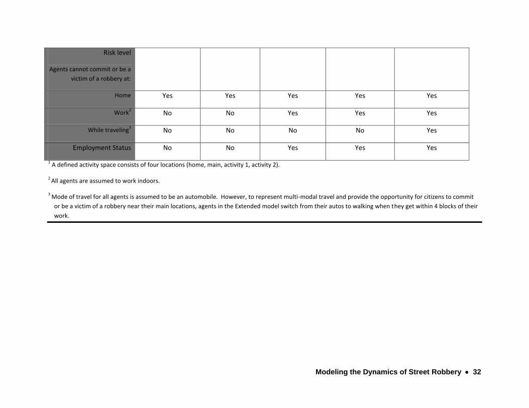
Table 2: Description of the Model Versions
Simple Grid Simple Street Temporal Activity Space Extended Model
Landscape Uniform Grid Street network Street network Street network Street network
Distribution of Civilians Random Random Random Assigned Assigned
Distribution of Police Random Random Random Random Random
Civilian Movement Random Random Random Defined Activity
Space1 (1 employed,
1 unemployed)
Defined Activity
Space1
(5 employed, 5
unemployed
Police Movement Random Random Random Random Random
Civilian Characteristics
Criminal Propensity Randomly assigned
to 20%
Randomly
assigned to 20%
Randomly assigned
to 20%
Randomly assigned
to 20%
Randomly assigned to
20%
Initial Wealth Randomly assigned Randomly
assigned
Randomly assigned Randomly assigned Based on income of
home block group
Pay Flat amount Flat amount Flat amount Flat amount Proportionate to
original wealth
Activity Space No No Temporal schedule Spatio-temporal Spatio-temporal
Modeling the Dynamics of Street Robbery 32
Risk level
Agents cannot commit or be a
victim of a robbery at:
Home Yes Yes Yes Yes Yes
Work2 No No Yes Yes Yes
While traveling3 No No No No Yes
Employment Status No No Yes Yes Yes
1 A defined activity space consists of four locations (home, main, activity 1, activity 2).
2 All agents are assumed to work indoors.
3 Mode of travel for all agents is assumed to be an automobile. However, to represent multi-modal travel and provide the opportunity for citizens to commit
or be a victim of a robbery near their main locations, agents in the Extended model switch from their autos to walking when they get within 4 blocks of their
work.

Modeling the Dynamics of Street Robbery 33
In order to test the impact of changes in routine activities on aggregate crime rates, the amount
of time spent away from home varies over five different experiments and across three different types of
activity spaces (no constraints, temporal constraints, spatio-temporal constraints) (Table 3). In other
words, each of the experimental conditions involves one type of activity space/constraint and one level
of time spent away from home (e.g. random movement when the society spends 40 percent of time
away from home vs. directed movement with spatio-temporal constraints when 40 percent of time is
spent away from home). Data on victimization are collected at the individual level and aggregated. The
first two hypotheses address the incidence of street robbery and the last two its spatial distribution:
H1: As the average time spent by civilians on activities away from home increases, the aggregate rate of robbery will increase.
H2: The temporal and spatio-temporal schedules of civilians while away from home change the incidence of robbery events.
H3: As the average time spent by civilians on activities away from home increases, the spatial pattern of robberies will change.
H4: The temporal and spatio-temporal schedules of civilians while away from home change the spatial pattern of robbery events.
The first hypothesis tests the core assertion of routine activity theory when agents have
temporal and spatio-temporal schedules. The second hypothesis examines the effect of adding
temporal and then spatio-temporally defined activity spaces on the incidence of street robbery.
The third hypothesis compares the outcome distributions of street robberies of the
experimental conditions (i.e. as society spends more time away from home) to one another.
The fourth hypothesis explores the impact of changing the structure of routine activities on the

Modeling the Dynamics of Street Robbery 34
spatial distribution of crime events. Since this is the first test of the effect of spatio-temporal
schedules on the spatial pattern of street robberies, hypotheses 3 and 4 do not describe the
potential outcome pattern but simply note it will be different.
These tests proceed in a systematic fashion, with each condition representing an
increase in the societal average for time spent on routine activities away from the home. All of
the percentages represent an average time spent away from home for the agent population as
a whole; individual agents have different times spent away from home.
Table 3: Experimental Conditions
Version of
Model
Average Time Spent Away From Home
C1 C2 C3 C4 C5
Grid Random 30% 40% 50% 60% 70%
Street Random 30% 40% 50% 60% 70%
Temporal 30% 40% 50% 60% 70%
Activity Space 30% 40% 50% 60% 70%
Extended AS 30% 40% 50% 60% 70%
Hours per week ≈50 ≈67 ≈84 ≈101 ≈118
Random number generators play an important dual role in agent-based models by
providing the stochastic elements in the model and enabling scientific experimentation. Both
uniform and normal random number distributions are used for decision-making in the model.
For example, random numbers play a key role in representing uncertainty in the current
knowledge about how individuals evaluate guardianship and target suitability. When a random
number seed is defined at the start of a simulation the random number generator produces the
Modeling the Dynamics of Street Robbery 35
same sequence of random numbers each time the model is run making experiments
repeatable. This characteristic forms the basis for using simulation as a laboratory for
experimentation because it enables any differences in the outcome variable to be attributed to
the manipulated variable and not to other sources (Aitken et al., 1989; Gold, 1980; Golledge &
Timmermans, 1990; Timmermans & Golledge, 1990; Walmsley & Lewis, 1993).
The five major components of the model: agent structure and characteristics, agent
behavior, agent activity spaces, model behavior, and landscape structure are addressed in the
Implementation Details section that appears next.
Implementation Details
Agent Structure and Characteristics
A complete description of the agents included in the model and their roles is necessary
before proceeding. There are two types of agents in the model: police officers and civilians.
Police officers have only one role while civilians can take on three different roles. The particular
role a civilian agent takes is driven by the contextual dynamics of the specific interaction.
Police officer agents are described first because of their relatively simple structure and
characteristics.
The only role of police officer agents is that of a formal guardian.17 Lack of a formal
guardian in routine activity theory is one of the elements that are necessary for a crime to
17 This research follows the strategy of making the model as simple as possible. Thus making the police officer agents one dimensional is one of many simplifying assumptions that are made in the model versions.
Modeling the Dynamics of Street Robbery 36
occur. Thus in the model, the presence of a police officer agent prevents a crime from
occurring. To accomplish their mission of crime prevention, police officer agents move one link
on the street network per minute of a day. This movement is random. Police officers never
commit crimes in this model and they are never targets. Officers in the model work 24 hours of
a day, 365 days a year. There are 200 police officers in each model version. This is a much
higher ratio that would be found in Seattle but it allows representation of the maximum effect
that police officers could be expected to have on street robbery. Manipulation of the number
of police officers is a fertile area of research with important policy implications and thus
deserves further exploration. For example, future studies could examine questions such as, if
we put a police officer on every corner, would we eradicate street robbery? 18
The civilian agents are members of the general population of the city. A civilian agent
can take on three types of roles: offender, target, or informal guardian. All civilian agents
within a model version follow the same basic set of rules. At the start of the simulation, all
civilian agents are randomly assigned an employment status, wealth level, criminal propensity
indicator, and an allocation of time to spend away from home. The constraints on spatio-
temporal activity spaces are determined by the model version.
The perception of an agent as a suitable target is an important aspect of routine activity
theory. Part of perception is the anticipated reward from robbing a particular target. To
accommodate this aspect, each civilian agent in the model is assigned an initial level of wealth
18 The assumptions of the model would have to be changed in order to test this hypothesis. Interestingly, a single model run in which there were the same number of police officers as citizens showed a decrease but not an eradication of crime..

Modeling the Dynamics of Street Robbery 37
and employed agents receive paychecks twice a month. Civilian agents are either employed or
unemployed. The employment status is randomly assigned to assume a 6 percent
unemployment rate. Every month, 3 percent of unemployed agents become employed and are
replaced by a new random selection of employed agents who become unemployed. It is
important to note that the employment status is assigned independently of the latent criminal
propensity indicator; civilians with criminal propensity can be employed in the model, as they
are in life. The methodology for assigning wealth is consistent across the four original models;
wealth is distributed using a normal distribution (mean=50, sd=30). Each employed agent
receives a flat paycheck of five units of wealth every other week.
Following routine activity theory, there is no attempt to model criminal motivation; it is
simply assumed to exist in some portion of the population. In order to ensure a constant level
of motivated offenders, 20 percent of the civilian agent population is assigned a “criminal
propensity” indicator. Agents with a criminal propensity designation will follow the same rules
as other civilian agents but will be the only civilian agents who evaluate each situation they
encounter and make the decision whether or not to offend based on guardianship and
availability of suitable targets. The specific structure of the decision to offend is outlined in the
section below on agent behavior. Thus the decision to commit an offense is a dynamic one and
contextually driven.
According to routine activity theory, it is the proportion of time spent away from home
during the course of routine activities that increases crime. In order to represent this concept
in the experiment, each of the civilian agents is randomly assigned percentages of time to stay

Modeling the Dynamics of Street Robbery 38
away from home so that the average for the model is a specific number. This assignment is
done using a normal distribution. For example, in the 40 percent scenario each of the civilian
agents would be randomly assigned a percentage of time to be away from home that would
result in a mean for the model of 40 percent (Table 4).
Table 4: Sample Assignment of Time Away From Home for 40 Percent Experimental
Condition
Status
Away*
At Home
Activity 1
or Work
Activity 2
Activity 3
Travel
Agent 1 U 26% 74% 20% 1% 2% 2%
Agent 2 E 45% 55% 24% 8% 7% 6%
Agent 3 E 60% 40% 26% 15% 9% 10%
Agent 4 U 81% 19% 24% 22% 30% 5%
Agent 5 E 53% 47% 30% 17% 3% 3%
Agent 6 U 30% 70% 3% 13% 10% 4%
Agent 7 U 25% 75% 10% 5% 2% 8%
Agent 8 U 11% 89% 8% 1% 1% 1%
Agent 9 E 41% 59% 30% 2% 4% 5%
Agent 10 E 28% 69% 24% 3% 1% 3%
Average 40% 60%
*Time ‘Away’ from home is the sum of the time spent at the three activity nodes. U = Unemployed, E = Employed
Agent Behavior
For each minute of the model, every agent with criminal propensity (one at a time)
considers the following aspects of a situation at a node (Figure 2: Model of Decision to Offend):
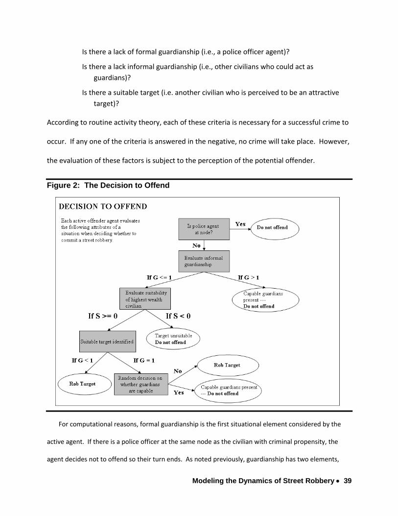
Modeling the Dynamics of Street Robbery 39
Is there a lack of formal guardianship (i.e., a police officer agent)?
Is there a lack informal guardianship (i.e., other civilians who could act as
guardians)?
Is there a suitable target (i.e. another civilian who is perceived to be an attractive
target)?
According to routine activity theory, each of these criteria is necessary for a successful crime to
occur. If any one of the criteria is answered in the negative, no crime will take place. However,
the evaluation of these factors is subject to the perception of the potential offender.
Figure 2: The Decision to Offend
For computational reasons, formal guardianship is the first situational element considered by the
active agent. If there is a police officer at the same node as the civilian with criminal propensity, the
agent decides not to offend so their turn ends. As noted previously, guardianship has two elements,

Modeling the Dynamics of Street Robbery 40
formal guardianship by police officer agents and informal guardianship by other agents at the node.
Informal guardianship is evaluated by counting the number of other civilian agents at the node and
subtracting one. This is necessary since the potential victim cannot be an informal guardian for
themselves. Uncertainty in how offenders perceive the ‘capableness’ of the other civilians is
incorporated into the formula through the addition of a stochastic term PG that can either increase or
decrease the active agent’s perception of the level of guardianship in a situation.
G = ((NA – 2) + PG) (1)
If G < 1, then there is a lack of capable guardians so condition evaluates to True
If G = 1, then make a random decision – condition could evaluate to True or False
If G > 1, then capable guardianship is present so condition evaluates to False
Where:
G = Guardianship
NA= number of agents at node
PG = Perception of capability of guardians who are present (uniform random number
between -2 and 2)
In reality, the presence of capable guardians is most likely evaluated along a continuum. On
one end of the continuum a police officer is present on the street corner. At the other end, the
potential offender is alone with a suitable target. More frequently, situations are somewhere
in between. It is likely that potential offenders are evaluating the potential guardianship of a
situation using a variety of criteria including presence of place managers (security guards,
parking lot attendants, etc.), number of other people on the street, characteristics of
neighborhood, etc. By incorporating a stochastic element in the potential offender’s decision-

Modeling the Dynamics of Street Robbery 41
making process in situations where there is some informal guardianship, the model is able to
more realistically represent uncertainty in how guardianship is evaluated.
Finally, the active agent considers whether there are suitable targets at the node. All other
civilians who are away from home and at the same node are evaluated using wealth as the
primary criteria for identifying a suitable target (2).
S = (WT) - (WA) + PS (2)
If S >= 0, then there is a suitable target so condition evaluates to True
If S < 0, then no suitable target present so condition evaluates to False
Where:
S = Perceived suitableness of target
WT = wealth of target
WA = wealth of active agent (potential offender)
PS = Offender perception of target suitability (uniform random value between -1 and 1)
If at least one other agent’s wealth exceeds the active agent’s wealth, the evaluation of the
civilian with the highest wealth continues via the formula above. The error term PS represents
the influence of other factors on the offender’s perception of the relative suitableness of a
target and its value can either increase or decrease the perceived suitability of the target. It is
worth noting that other agents with criminal propensity who are at the node are included in the
active agent’s evaluation and can become victims. If S < 0, there is not suitable target at the
node, and the active agent does not commit robbery.

Modeling the Dynamics of Street Robbery 42
To recap, for situations in which there is a suitable target, the decision to offend hinges on
the level of informal guardianship. If G < 1, then there is there is a lack of capable guardians so
the decision is to rob the suitable target identified. If G > 1, the amount of guardianship is too
high, and the decision is not to offend. But if G = 1, the decision could go either way. In these
cases, the active agent makes a random decision whether to commit the street robbery. When
an agent commits a robbery, one unit of wealth is taken from the victim and transferred to the
offender. Once each civilian with criminal intent has evaluated their situation, the model time
advances, agent properties (i.e., wealth, victimizations, offenses etc.) are updated, agents
move, and the decision structure is repeated.
Model Behavior
In addition to the behavior of civilians and police officers, there are several general rules
of behavior that underpin the structure of the model. During each minute of the model run and
in random order, every agent with ‘criminal propensity’ (i.e., a potential offender) evaluates
their situation using the equations defined in section 3.4. Only the agents with ‘criminal
propensity’ are able to make the decision to offend. The role a civilian agent takes in each turn
is dynamically determined by the presence or absence of a police officer and the number and
relative wealth of the other civilian agents. Any civilian agent can play the role of suitable
target or informal guardian depending on the other agents present.
Landscape Structure
Two types of landscapes are used depending on the version of the model. A uniform
grid serves at the landscape for the Simple Grid version. The uniform grid has 15,975 nodes

Modeling the Dynamics of Street Robbery 43
which makes its density very similar to the overall density of the street network in Seattle.19
Each node on the grid is analogous to a street corner and each link is analogous to a street
segment. The uniform grid version serves a critical function in the modeling process; it serves as
a null model to the rest of the model versions by supplying a ‘random’ outcome to which we
can compare outcomes that use parameters of interest such as the street network. By
comparing the results of the Simple Grid to those of the Simple Random version we can say
exactly how much effect using a GIS-based street network has on the results of the model. In
addition, any differences in emerging patterns can be attributed to the change in landscape.
The rest of the versions all use the Seattle street network which consists of 16, 035 nodes (i.e.,
street intersections).20
Creating Activity Spaces for the Civilian Agents in the Model
One of the core concepts in routine activity theory involves the necessity of the
convergence of victims and offenders in space and time. The specific ‘where’ and ‘when’ of
convergence stems from the routine behavior patterns of each actor involved. Thus
representing the spatio-temporal aspects of human behavior that facilitate convergence is a
critical element in modeling street robbery events since it is the interactions between humans
and their environment that serve as the source of explanation of observed spatial patterns
(Horton & Reynolds, 1971).
19 The uniform grid was generated in ArcGIS 9.2.
20 Please see Appendix A for the technical details that necessitated the use of street intersections rather than street segments as the basic travel landscape. Appendix A also contains the details of creating
Modeling the Dynamics of Street Robbery 44
A large quantity of research is available to inform agent movement and routine activities
in the model and that research suggests people tend to have an area within which they conduct
their daily activities. Some researchers term this area an activity space (Miller, 1991), some call
it a potential path area (Hägerstrand, 1970, 1975), and others a domain (Hägerstrand, 1970,
1975). This area encompasses both the locations that are visited and the paths taken among
those locations. Different perspectives have their own terms for these locations and paths.
Locations that are visited are called stations (P. J. Brantingham & P. L. Brantingham, 1981; P. L.
Brantingham & Brantingham, 1993; Lynch, 1960; Miller, 1991), nodes (Golledge, 1978; Golledge
& Stimson, 1997), or anchorpoints (Hägerstrand, 1970, 1975; Lynch, 1960). These are the
places where the majority of human interaction occurs. The particular routes taken among the
locations are termed paths (Hägerstrand, 1970). None of these elements are static, for
example, the shape and size of areas (i.e. activity spaces) can change as people change jobs (i.e.
nodes) or as their circumstances change (E. R. Groff, 2008b).
Regardless of the terminology, home tends to be the dominant place in any activity
space. Travel tends to be concentrated along certain routinely frequented paths. Frequently
traveled paths may be important factors in determining aggregate crime patterns because they
bring offenders and victims together in space and time. Individual’s travel patterns are
influenced by constraints (i.e., temporal, economic and spatial) on their ability to take
advantage of opportunities for housing, employment, recreation etc
a landscape and activity spaces as well as more information on agent movement along a vector network..

Modeling the Dynamics of Street Robbery 45
Together this collection of research provides a strong basis for conceptualizing routine
activity spaces of individuals as a set of places and the paths between those places. Five types
of activity spaces are included in the model; each adds complexity and is associated with a
different version of the model: Grid Random, Street Random, Temporal, Activity Space, and
Extended Activity Space (previously described in Table 2). In two of the model versions (i.e.,
Grid Random and Street Random) civilians travel randomly and either at home (i.e., not at risk)
or not at home (i.e., at risk). Agents assigned to a random movement pattern move randomly
from node to node. They are randomly distributed at the beginning of the simulation and begin
the next day at the node where they ended the previous one. The Temporal version adds a
temporal schedule that changes the risk level of the agent to reflect their activity but retains
random travel. In the other two versions they have a directed travel route that reflects a
defined activity space (i.e., Activity Space and Extended Activity Space).
Agents in the directed movement versions (i.e., with defined activity spaces) always
begin a model day at their home. They have a total of four places in each of their activity
spaces consisting of a home, main (workplace if employed or main hangout otherwise), and two
recreation nodes. The term recreation is used loosely to represent grocery stores, coffee
shops, gyms, retail stores, parks etc. Agents always take the shortest path between assigned
nodes and the path among assigned places is calculated using a geographic information system
prior to the model run.
In the Activity Space version, routine activity spaces are implemented as a set of nodes
(places) and paths (list of places traversed when traveling from one node to another). See
Modeling the Dynamics of Street Robbery 46
Appendix 1 for the technical details of how activity spaces were created. As in life, each agent
has a routine activity space that consists of a set of places that are visited each day.
Specifically, each civilian agent is assigned four places representing a home, a main activity
(e.g., work, school etc.) and two other activities (e.g., recreation, social, and retail places). The
places are assigned based on the distributions of population, jobs and activities in Seattle (e.g.,
if 10% of the population lives in a particular block group then 10% of the agents are assigned to
that block group) (O'Sullivan, 2004; Oreskes, Shrader-Frechette, & Belitz, 1994). In this way, the
size and form of activity spaces is influenced by the distribution of residential housing, jobs,
schools, retail and services.21 Activity Space agents have two potential activity; one activity
space to use while employed and another while unemployed. Employed and unemployed
activity spaces are identical except that the work location is dropped from the unemployed
path and a new activity location is added.
In order to incorporate travel time into the daily routine (i.e., Temporal, Activity Space and
Extended Activity Space versions), the total travel time among assigned nodes is calculated and
subtracted from the total available for allocation. The remaining time is then allocated among
the four nodes. The time to be spent at home (allocated earlier in the model) is subtracted
from the remaining time. Finally, time spent at work and the two recreation nodes is assigned
using a random distribution. For employed agents, one location is work and the other two are
recreation locations. Unemployed agents have three recreation locations. When an agent’s
21 The agent activities are attached to a series of street intersections rather than street addresses or street blocks. The use of street intersection reflects a software limitation. Repast cannot read network or geodatabase files from ArcGIS.

Modeling the Dynamics of Street Robbery 47
employment status changes, the work node is either added or subtracted (and replaced by a
new activity node) and the allocation of time is recalculated. The agents’ initial travel
destination is based on their daily routine. Civilian agents proceed along travel nodes, in doing
so they pass along the same network and nodes as other civilians and as police officer agents.
As previously noted, the average time spent away from home is systematically varied in each of
the five experimental conditions but is randomly allocated to individual civilian agents within
each experimental condition.
One difference between the original four models and the Extended Activity Space version is
that under the original versions a traveling agent could perpetrate or become victims of a crime
but under the Extended Activity Space version they are not at risk while traveling. The only
exception is when employed agents are near (within four blocks of) their work place they
switch to walking and thus are at risk of street robbery. This is necessary to reflect some risk at
workplaces. Otherwise, the trip to work would involve no risk since they would be traveling to
and from the location by car and then be inside once they arrived.
Absolute risk of committing or being a victim of a street robbery is closely tied to the
temporal and spatio-temporal aspects of activity spaces. Civilians in the Temporal, Activity
Space and Extended Activity Space models share the same temporal schedule for activities and
travel and consequently those agents spend the same amount of time ‘at risk’ for street
robbery. Employment status also affects risk in the Temporal and Activity Space versions of the
model by changing the amount of time spent at the three activity nodes (but not the overall
time spent away from home) and the amount of wealth that an agent receives. In the case of

Modeling the Dynamics of Street Robbery 48
the Activity Space version, employment status also determines the spatial configuration of the
agent’s activities (i.e., the locations of the places that are visited).
Challenges to Learning from Models: Calibration and Validation Before turning to the results of the theoretical experiments outlined here, it is prudent
to examine some of the challenges in learning from simulation models especially those for
which prediction is the goal. The main challenge is termed the equifinality problem and is not
unique to simulation but involves all numerical models (2004). The equifinality problem
concerns the fact that more than one model can produce the same result. Thus, even the best
calibrated and most rigorously tested models can account for the same observed outcome
using different mechanism. In response, O’Sullivan (O'Sullivan, 2004, pp., 291) suggests the
following approach.
“It is clear that assessment of the accuracy of a model as a representation must rest on argument about how competing theories are represented in its workings, with calibration and fitting procedures acting as a check on reasoning. So, while we must surely question the adequacy of a model that is incapable of generating results resembling observational data, we can only make broad comparisons between competing models that each provide ‘reasonable’ fits to observations. Furthermore, critical argument and engagement with underlying theories about processes represented in models is essential: no purely technical procedure can do better than this.” (Batty & Torrens, 2005)
Another challenge to validating simulations of crime is lack of a reliable dependent
variable (Eck & Liu, 2008a). Official crime data are most frequently used but they reflect an
unknown fraction of the actual crime events that occur. A simulation model is set up to
generate actual numbers of crime; as if all crimes were reported by victims and all were judged

Modeling the Dynamics of Street Robbery 49
valid by police. Thus simulation models are built to reflect all crime while official crime data
captures an unknown portion of total crimes committed. In this situation, we could build the
correct simulation model to predict all crime (i.e., reported crime + ‘dark figure’ of crime) and it
would look incorrect when compared with official crime data.
An alternate approach is to evaluate the plausibility of the patterns and numbers of
crime produced by models. Under this standard, model results are judged on how well they
reproduce the general characteristics of crime patterns and volume (Eck & Liu, 2008a; Liu et al.,
2005). Specifically, to be credible the crime patterns produced would have to have the
following characteristics: 1) spatially concentrated rather than dispersed (i.e., a few locations
should have many crimes and many locations should have just a few); 2) include both repeat
offenders and repeat victims; and 3) have a similar magnitude (Batty & Torrens, 2005; Dowling,
1999; O'Sullivan, 2004; Oreskes et al., 1994).
The potential for learning is a product of the entire model building process from
formalization of theories, to sensitivity testing and calibration, to comparison with observed
data: under this framework models are heuristic devices, representations that can aid in
understanding and illuminate mechanisms at work for further study (Manson, 2001; O'Sullivan,
2004). Although the current research emphasizes the representation of theory in models, and
how we can learn from that process, it also takes issues of calibration and validation seriously
and these are discussed next.i Choices of the parameter values and distributions used in the
model are included under the rubric of calibration. Explorations of the parameter space assist
with the understanding of mechanisms at work in the model. While the concept of validation is

Modeling the Dynamics of Street Robbery 50
centered on the level of confidence we can have in a model, namely do both the mechanisms
and the results of the model reflect reality (or at the very least the reality of imperfect data).
Validation involves comparing model results to actual data.
Related to calibration, the choice of parameter values is a critical aspect of modeling
that deserves special attention because of the potential impacts on the model outcomes.
Modelers try to use theoretically-based empirical values whenever possible and plausible ones
when empirical ones are not available. Some modelers use sensitivity testing to quantify the
robustness of the model results (Liu et al., 2005, 208; Oreskes et al., 1994). This is
accomplished by systematically varying the initial parameters and the random number seed
and testing the impact on the model results. Others use calibration to “fit a real data set”
(Axelrod, 2006). In this process, the parameters are systematically changed to attempt to
match the empirical data pattern and intensity.
This study evaluates the robustness of the findings through the systematic variation of
five of the key parameter values and by varying the random number seed used across the new
versions of the model. The five parameter values are systematically increased (i.e. number of
police, time to wait before able to re-offend, initial wealth distribution, perception of target
suitability random term, and the perception of guardianship random term), the model runs are
repeated for all five experimental conditions, and a one-way ANOVA (ANalysis Of VAriance) is
applied to analyze the results. Finally, the entire sensitivity testing process of varying the five
parameter values is repeated four more times using different random number seeds to test the
effect of changing the random number seed on the outcomes of the model.

Modeling the Dynamics of Street Robbery 51
Sensitivity testing demonstrates the original and the new model versions are robust to
changes in parameters and random number seeds. The absolute number of robberies increased
or decreased depending on the parameter being varied. However, findings related to routine
activity theory’s core proposition remain consistent across the vast majority of the tests lending
additional support for robustness of the model even as parameters are varied. The two
exceptions are found in one of the random number seed tests and the time spent away from
home. One of the random number seed variations produces a significant result for the Activity
Space version. Otherwise, the results of the model are shown to be robust to changes in the
random number seed. Increasing the time an agent with criminal propensity has to wait to
commit another street robbery makes the ANOVA for the Temporal version non significant and
points to the importance of timing in the decision to offend.
Analysis Both traditional and spatial analysis techniques are used to examine the results of the
model runs. Descriptive statistics such as mean, median and standard deviation are used to
characterize the results of each of the experiments. As is customary practice, an ANOVA is
applied to determine if there is a significant difference among the robbery rates (RobRate) for
the five experimental conditions(Bailey & Gatrell, 1995; Mitchell, 1999; Williamson et al., 2001).
In an ANOVA, the mean number of street robberies for all the citizens in the model are
compared across experimental conditions. If the differences are significant, then we can say
with some confidence that as time spent away from home increases, crime also increases. The
number of robbery victimizations for each civilian agent in the model is the response variable.
Modeling the Dynamics of Street Robbery 52
A sample size of five thousand observations across five experimental conditions provides a very
powerful design. Thus increasing the sample size to ten thousand or twenty thousand should
not change any findings of significant differences among the groups. Finally, the resulting
spatial patterns of robbery events are examined.
At the agent level, descriptive statistics are generated to test the relationships among
time spent away from home (AwayTime), total number of victimizations (TotVict), and total
number of robberies committed (TotOff). These statistics are examined for the total population
and then just for agents with and without criminal propensity. These measures are collected
via log files that can be instructed to collect additional information to inform future research.
These log files are then imported into a spreadsheet (Excel) and a statistical package (SPSS) for
further analysis.
Two approaches to describing the spatial distribution of street robberies are taken. A visual
comparison is made of the resulting crime patterns using a kernel density. Kernel density
surfaces offer a means of evaluating the existence of global trends in the distribution of street
robberies and for comparing the relative density of robberies across experimental conditions.
To create a kernel density, a temporary grid is laid over the entire study area and a density
value for each cell in the grid is computed using a circular ‘neighborhood’ (Bailey & Gatrell,
1995; Levine, 2005).22
22 The term kernel refers to size of the ‘neighborhood’ (also called bandwidth) that is taken into account when computing the density. The total number of street robberies within the bandwidth are summed and divided by the area under the circle. The resulting value is assigned to the current cell.

Modeling the Dynamics of Street Robbery 53
In addition to the kernel density, formal tests of the spatial distribution of crime events are
employed using Ripley’s K function. The total numbers of robberies, robberies deterred, and
agents who visit are collected for each node in the network. Ripley’s K is applied to compare
the clustering of robberies and visits to places at different scales. Typically, the K function for
complete spatial randomness (CSR) is helpful in identifying whether the observed pattern is
significantly different than what would be expected from a random distribution (Levine, 2005).
A known weakness of comparing the observed distributions to CSR is that most human-
generated patterns are non-random (e.g., population, housing, etc.) (Eck, Gersh, & Taylor,
2000; Sherman, Gartin, & Buerger, 1989; Weisburd, Bushway, Lum, & Yang, 2004).
In this research, CSR cannot be used to evaluate the clustering in street robbery events
because the locations at which data are collected are constrained to a fixed set of locations
representing the intersections in Seattle.23 Since the CSR algorithm randomly places points
anywhere within the study area boundary, it would be inappropriate to compare the clustering
in robberies and number of visits, which are constrained to the street nodes, to a randomly
generated CSR. However, a K function can be generated from the pattern of street nodes thus
revealing the extent of the clustering intrinsic to the street network. Comparing the K function
for street intersections to CSR answers the question of whether the intersections are more
clustered than would be expected under CSR. Taking this one step further, the K function for
street robberies can be compared to the one for intersections to find out if robberies are more
clustered than the street intersections.
23 Thanks to Ned Levine for pointing out this issue.
Modeling the Dynamics of Street Robbery 54
Another aspect of the same discussion involves the role of the street nodes in structuring
the initial distribution of police and civilians since they too can only be allocated to a street
node (and not to any location within Seattle). In this way, the structure of the street network
conditions both the original distribution of agents and their movement. Since the agents are
randomly assigned to nodes and they move randomly during the simulation, the distribution of
robberies should be similar to that of the network nodes if space alone determines where
street robberies occur. To check this, the K function for nodes is compared to the K functions
for both robberies and visits.
The impact of schedule constraints on the spatial distribution of street robbery is evaluated
by comparing the findings from the Simple version to those from the Temporal and Activity
Space versions across the five experimental conditions using kernel density and Ripley’s K. All
of these measures are distance-based and characterize the spatial patterning of the street
robbery locations as conditioned by the pattern of street nodes. The robustness of all the
findings is then evaluated through the systematic variation of five of the key parameter values
and by varying the random number seed used across the new versions of the model.
Findings This section summarizes the findings of the analyses just described. First descriptive
model outcomes are expressed by examining both place- and societal-level attributes to
characterize differences in the results from the model runs of the five versions across the five
experimental conditions. Next, the results pertinent to each of the hypotheses are discussed.

Modeling the Dynamics of Street Robbery 55
Descriptive Analysis
This successful implementation of a theoretically-based, geographically-aware model of
street robbery capitalizes on the recent development of Agent Analyst which allow a simulation
model to be ‘situated’ on an extant rather than an artificial landscape and in doing so provides
a more realistic context to the model behavior. However, the effect of ‘situating’ simulation is
an open question. This research quantifies the impact of realistic landscapes by comparing the
differences in the incidence and pattern of street robberies when the same model is run on a
uniform grid versus an actual street network. Societal level changes in the number of street
robberies, the frequency of convergence of agents in space-time (i.e. opportunities for street
robbery), and the number of crimes deterred by the police for all versions of the model are in
line with what routine activity theory would expect; all the values increase steadily with time
spent away from home (Table 5). While the overall trends across models are consistent,
significant differences in volume exist by model version. The results from each version are
summarized and then compared.
The Street Random version has the highest number of robberies and the steepest
increases as time spent away from home increases. The Grid Random version has the next
highest number of street robberies although both versions are significantly higher than either
the Temporal or Activity Space versions of the model. Temporal version has the fewest
robberies and an identical slope as the Activity Space version. Together these results point to
the importance of the street network to increasing robbery by increasing the number of
convergences. They also illustrate the critical role of a time schedule in lowering the incidence
of street robberies regardless of the time spent away from home. The addition of a spatially-

Modeling the Dynamics of Street Robbery 56
constrained schedule to the Temporal version increases the number of street robberies. This
outcome is most likely related to the rate of convergence (i.e. presence of motivated offender
and suitable target at same place-time) which tends to be highest in the Activity Space version
and lowest in the Temporal version.
Results from this research also show that deterrence (i.e. number of times the presence
of a police agent prevents a robbery from taking place) increases for all model versions as the
societal time spent away from home increases and the relationships among the versions are
identical to those for convergence. This supports Cohen and Felson’s (1979) hypothesis that
the frequency of convergence impacts the potential for deterrence. Whenever there are more
convergences there are by definition more times a police agent can function as an agent of
formal guardianship.
These findings illustrate the separate impact of a temporal schedule and a defined
activity space on the frequency of convergences across the three models. Agents who travel
randomly but have a temporal schedule experience the fewest number of convergences
because the time they are ‘at risk’ is less than the agents in the Simple version. When a spatial
element is added (i.e. agents have defined activity spaces), it increases the frequency of
convergence because agent’s homes, jobs and activities are clustered as opposed to randomly
allocated across Seattle as in the other versions. Increasing convergence translates into more
street robberies for agents in the Activity Space version.
Beginning with the comparison of the same model on a grid landscape versus a street
network, the results clearly demonstrate that the street network itself has a measurable effect

Modeling the Dynamics of Street Robbery 57
on the number and pattern of street robberies. When situated on a street network, society
experiences roughly ten percent more convergences and robberies than when it exists on a
uniform grid (Table 5). This outcome is most likely due to the funneling effect of the street
network on human activity; it increases the number of times people converge.

Modeling the Dynamics of Street Robbery 58
Table 5: Societal-level Model Outcomes
Experimental Condition
30% 40% 50% 60% 70%
Target time to spend away
from home, minutes
(hours)
432
(7.2)
576
(9.6)
720
(12)
864
(14.4)
1008
(16.8)
Actual time spent away
from home
437.2 (G)
436.9 (S)
427.8 (T)
427.7 (AS)
580.2 (G)
580.2 (S)
572.5 (T)
572.3 (AS)
723.5 (G)
723.5 (S)
717.0 (T)
716.9 (AS)
866.8 (G)
866.8 (S)
861.6 (T)
861.5 (AS)
1010.1 (G)
1010.1 (S)
1006.2 (T)
1006.2 (AS)
Total Robberies 50,373 (G)
54,637 (S)
12,807 (T)
32,326 (AS)
68,624 (G)
76,032 (S)
13,671 (T)
34,628 (AS)
87,458 (G)
95,219 (S)
15,183 (T)
38,331 (AS)
106,317 (G)
118,085 (S)
16,196 (T)
41,266 (AS)
124,902 (G)
139,007 (S)
17,181 (T)
46,085 (AS)
Total Convergences 1,324,238 (G)
1,454,341 (S)
736,787 (T)
1,889,899 (AS)
1,839,695 (G)
2,050,761 (S)
1,013,814 (T)
2,663,961 (AS)
2,366,854 (G)
2,631,149 (S)
1,285,568 (T)
3,446,132 (AS)
2,878,678 (G)
3,238,760 (S)
1,579,963 (T)
4,260,133 (AS)
3,404,249 (G)
3,835,299 (S)
1,880,647 (T)
5,018,754 (AS)
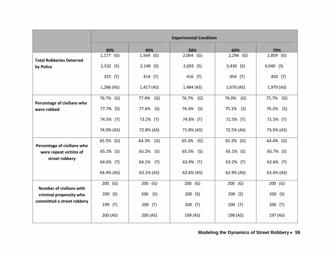
Modeling the Dynamics of Street Robbery 59
Experimental Condition
30% 40% 50% 60% 70%
Total Robberies Deterred
by Police
1,177 (G)
1,532 (S)
325 (T)
1,286 (AS)
1,564 (G)
2,148 (S)
414 (T)
1,417 (AS)
2,064 (G)
2,693 (S)
416 (T)
1,484 (AS)
2,296 (G)
3,430 (S)
454 (T)
1,670 (AS)
2,859 (G)
4,040 (S)
450 (T)
1,979 (AS)
Percentage of civilians who
were robbed
76.7% (G)
77.7% (S)
74.5% (T)
74.0% (AS)
77.4% (G)
77.6% (S)
73.2% (T)
72.8% (AS)
76.7% (G)
76.4% (S)
74.6% (T)
71.8% (AS)
76.0% (G)
75.1% (S)
72.5% (T)
72.5% (AS)
75.7% (G)
76.2% (S)
71.5% (T)
73.5% (AS)
Percentage of civilians who
were repeat victims of
street robbery
65.5% (G)
65.2% (S)
64.6% (T)
64.4% (AS)
64.3% (G)
65.2% (S)
64.1% (T)
63.1% (AS)
65.3% (G)
65.5% (S)
63.9% (T)
62.6% (AS)
65.2% (G)
65.1% (S)
63.2% (T)
62.9% (AS)
64.4% (G)
65.7% (S)
62.6% (T)
63.4% (AS)
Number of civilians with
criminal propensity who
committed a street robbery
200 (G)
200 (S)
199 (T)
200 (AS)
200 (G)
200 (S)
200 (T)
200 (AS)
200 (G)
200 (S)
200 (T)
199 (AS)
200 (G)
200 (S)
200 (T)
198 (AS)
200 (G)
200 (S)
200 (T)
197 (AS)

Modeling the Dynamics of Street Robbery 60
(G) Grid Random (S) Street Random (T) Temporal (AS) Activity Space (EAS) Extended Activity Space

61 Modeling Street Robbery
A comparison of the Street Random version to the Temporal version reveals even
more striking differences. When time constraints and their associated variation in risk
status are added to the model the number of robberies declines by precipitously at 30%
time spent away from home. This decrease clearly demonstrates the importance of
time people are at risk as an important factor in crime rates. There are also far fewer
convergences of motivated offenders and potential targets because agents are at risk of
victimization/offending less. There is only slight variation in the percentage of agents
that are victims and repeat victims of crime so the change must be in the degree of
victimization among those agents who are repeat victims; the number of victimizations
among repeat victims is lower in the Temporal version.
Comparing the Temporal version with the Activity Space version reveals even more
striking differences. This comparison specifically examines the effect of considering the
distribution of opportunities via routine activity spaces on street robbery. In the Street
Directed travel version, the number of convergences increases by 27 percent (Table 5).
Agents are coming into contact more frequently because their activities reflect the
clustered nature of opportunities and because those activities are routine rather than
random. However, both the number of street robberies and percentage of civilians who
are robbed decrease in the Street Directed version. This seeming anomaly is due to the
following process, as citizens with criminal propensity get more wealth than those
without, fewer crimes occur because there are fewer suitable targets.

62 Modeling Street Robbery
Spatial Pattern Differences
In addition to differences in the absolute number of robberies among the model
versions, the patterns of street robberies produced by the model versions are markedly
different. If we look at the distribution of crime in the street random model we see a
skewed distribution with most places having relatively few robberies (Figure 3).
However, there are slightly more places with two robberies than with one (a finding that
is not consistent with real crime distributions).
Figure 3: Frequency Distribution of Street Robberies from Street Random
Version
In contrast, the distribution of crime across places in the grid random version is even
less like the typical empirical crime distribution. While still right skewed, it is much less
skewed than the output from the Street Random version and could be termed a

63 Modeling Street Robbery
truncated normal (Figure 4). There are fewer places with 0, 1, or 2 robberies than with
three robberies. The crime pattern generated from the grid landscape is very dispersed
with about 94 percent of all nodes experiencing at least one street robbery as compared
to the only about 83 percent of street nodes.
Figure 4: Frequency Distribution of Street Robberies from Grid Version
The frequency of street robberies across places from the Temporal version has a
more traditional shape (Figure 5). The number of robberies drops very off quickly as the
number of places increases.

64 Modeling Street Robbery
Figure 5: Frequency Distribution of Street Robberies from Temporal
Version
The activity space model comes closest to a realistic distribution of crime across
places (Figure 6). The number of places with only one robbery is the highest and drops
off quickly. Very few places have very high numbers of robbery events.

65 Modeling Street Robbery
Figure 6: Frequency Distribution of Street Robberies from Street Directed
Version
Hypotheses
The purpose of the model creation was to test four different hypotheses. The
results of those tests are discussed next.
Hypothesis 1: As the average time spent by civilians on activities away from home
increases, the aggregate rate of robbery will increase.
A One-Way ANOVA is applied to the means of the five experimental conditions
to determine if the average number of robberies increases as the time spent away from
home increases. The results of the ANOVA indicate significant differences for the Grid

66 Modeling Street Robbery
Random, Street Random and Temporal versions (Table 7).24 So overall, only the results
of the Activity Space version did not support routine activity theory’s core proposition.
24 Because of the positive skew to the distribution of robberies, additional tests regarding the equality of means are conducted. Both the Brown-Forsythe and the Welch tests for equality of the means are significant at .000. These tests are preferable to the F test when the equality of variances assumption is violated as it is here (Newton & Rudestam, 1999; Shannon & Davenport, 2001).

67 Modeling Street Robbery
Figure 7: ANOVA for Street Robbery Events across Versions and
Experimental Conditions
Proportion of Time Spent Away From Home
Condition
1
(30%)
Condition
2
(40%)
Condition
3
(50%)
Condition
4
(60%)
Condition
5
(70%)
Number of civilians N=1,000 N=1,000 N=1,000 N=1,000 N=1,000
Grid Random ***
Mean
(Standard Deviation)
50.37
(93.36)
68.62
(129.08)
87.46
(166.46)
106.32
(204.25)
124.90
(241.19)
Street Random ***
Mean
(Standard Deviation)
54.64
(101.99)
76.03
(144.15)
95.22
(182.35)
118.09
(228.14)
139.01
(270.06)
Temporal Model ***
Mean
(Standard Deviation)
12.81
(17.54)
13.67
(19.35)
15.18
(22.42)
16.20
(24.34)
17.18
(26.64)
Activity Space Model
Mean
(Standard Deviation)
32.33
(87.69)
34.63
(103.26)
38.33
(129.42)
41.27
(148.5)
46.09
(174.90)
*** Difference among one or more of the groups is significant at P <= .000.

68 Modeling Street Robbery
Additional tests using Tamhane’s T2 are employed to identify which groups
differed significantly (Table 8).25 Comparing each group, in turn, to the other four
groups reveals that there are differences between the conditions in the Grid Random,
Street Random and Temporal versions.26 While all but two comparisons for the Grid
Random and Street Random versions were significant, only three of the between-group
differences are significant for the Temporal version; between the 30% and both the 60%
and 70% conditions as well as between the 40% and the 70% condition. Thus, the effect
of a temporal activity schedule is to reduce the number of significant differences
between the experimental conditions.
25 Tamhane’s T2 is used because it does not assume equal variances. A test for homoscedasticity showed the variances are not equal across the five experimental conditions. The Levene statistic is significant indicating the variances are significantly different among the groups. However, ANOVA is robust in the face of this violation when the group sizes are equal which they are in this research (Calthrope, 1993; Duaney & Plater-Zyberk, 1993; Nelessen, 1994).
26Tamhane’s T2 is only applied to those versions in which there were significant differences for the version as a whole.

69 Modeling Street Robbery
Figure 8: Post Hoc Tests of Mean Differences by Experimental Condition
(seed = 100)
(I) Randomization
Condition
(J) Randomization
Condition
Mean difference
(I - J)
Standard
error
Significance
30% Time away 40% Time away
(G) a -18.25 5.04 .003
(S) a -21.39 5.58 .001
(T) -.86 .83 .970
50% Time away
(G) a -37.09 6.04 .000
(S) a -40.58 6.61 .000
(T) -2.38 .90 .081
60% Time away
(G) a -55.94 7.10 .000
(S) a -63.45 7.903 .000
(T) a -3.39 .949 .004
70% Time away
(G) a -74.53 8.18 .000
(S) a -84.37 9.13 .000
(T) a -4.37 1.01 .000
40% Time away 50% Time away
(G) a -18.83 6.66 .046
(S) -19.19 7.351 .088
(T) -.51 .936 .676
60% Time away

70 Modeling Street Robbery
(G) a -37.69 7.64 .000
(S) a -42.05 8.534 .000
(T) -2.53 .983 .098
70% Time away
(G) a -56.28 8.65 .000
(S) a -62.98 9.681 .000
(T) a -3.51 1.041 .008
50% Time away 60% Time away
(G) -18.86 8.33 .213
(S) -22.87 9.236 .126
(T) -1.01 1.046 .983
70% Time away
(G) a -37.44 9.27 .001
(S) a -43.79 10.305 .000
(T) -2.00 1.101 .515
60% Time away 70% Time away
(G) -18.59 9.99 .479
(S) -20.92 11.180 .470
(T) -.98 1.141 .993
a Significant differences were found between experimental conditions I and J at p < .05.
H2: The temporal and spatio-temporal schedules of civilians while away from home
change the incidence of robbery events.
This hypothesis explores whether the versions of the model produce significantly
different numbers of street robberies for each of the experimental conditions (e.g.

71 Modeling Street Robbery
whether the number of robberies under the 30% time away condition for the Street
Random version were significantly different than those under the Grid Random,
Temporal, or the Activity Space versions). The results of the ANOVA indicate there are
significant differences between the rates of street robbery for four versions of the
model. However, a post hoc analysis reveals the differences between the Grid Random
and Street Random models were not significant under any experimental condition.
While the differences between those two models and the Temporal and Activity Space
models were significant under all five experimental conditions (Table 9). In other words,
regardless of the amount of time spent away from home or landscape type, including
the temporal and spatial components of activity spaces resulted in significantly different
robbery rates. These results support the separate importance of both time, and space
when modeling routine activities.

72 Modeling Street Robbery
Table 9: Post Hoc Tests of Mean Differences Between the Same
Experimental Condition in Different Model Versions (Seed = 100)
(I) Version (J) Version Mean difference
(I - J)
Standard
error
Significance
Street Random Temporal
30% Time Away a 41.83 3.272 .000
40% Time away a 62.36 4.599 .000
50% Time away a 80.84 5.810 .000
60% Time away a 101.89 7.255 .000
70% Time away a 121.83 8.582 .000
Activity Space
30% Time Away a 22.31 4.253 .000
40% Time away a 41.40 5.607 .000
50% Time away a 56.89 7.071 .000
60% Time away a 76.82 8.608 .000
70% Time away a 92.92 10.175 .000
Grid Random
30% Time Away 4.26 4.37 .909
40% Time away 7.41 6.12 .785
50% Time away 7.76 7.81 .901
60% Time away 11.77 9.68 .782
70% Time away 14.11 11.45 .772
Temporal Activity Space
30% Time Away a -19.52 2.828 .000
40% Time away a -20.96 3.322 .000
50% Time away a -23.15 4.154 .000

73 Modeling Street Robbery
60% Time away a -25.07 4.758 .000
70% Time away a -28.90 5.594 .000
Grid Random
30% Time Away a -37.57 3.00 .000
40% Time away a -54.95 4.13 .000
50% Time away a -72.28 5.31 .000
60% Time away a -90.12 6.51 .000
70% Time away a -107.72 7.67 .000
Activity Space Grid Random
30% Time Away a -18.05 4.05 .000
40% Time away a -34.00 5.23 .000
50% Time away a -49.13 6.67 .000
60% Time away a -65.05 7.99 .000
70% Time away a -78.82 9.42 .000
a Significant differences were found between model versions I and J at p < .05.

74 Modeling Street Robbery
H3: As the average time spent by civilians on activities away from home increases, the
spatial pattern of robberies will change.
A tabular view of the spatial distribution of agent movement and robberies offers
descriptive evidence in support of this hypothesis (Table 10). The outcome measures reveal
both increases in concentration and spread of street robberies as time spent away from home
increases. Mean robberies per node are lowest in the Temporal model followed by the Activity
Space model. For all the model versions, as time spent away from home increases, the
percentage of places with one or more robberies and the percent of places with more than one
robbery increase steadily.
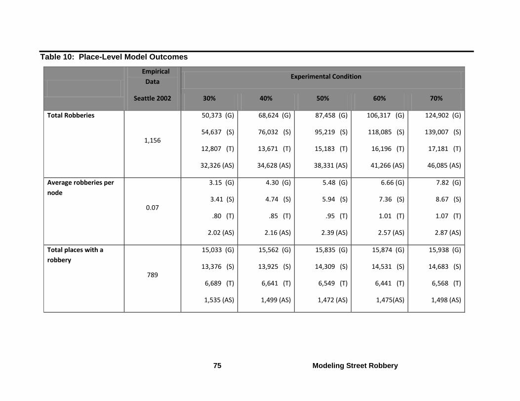
75 Modeling Street Robbery
Table 10: Place-Level Model Outcomes
Empirical
Data Experimental Condition
Seattle 2002 30% 40% 50% 60% 70%
Total Robberies
1,156
50,373 (G)
54,637 (S)
12,807 (T)
32,326 (AS)
68,624 (G)
76,032 (S)
13,671 (T)
34,628 (AS)
87,458 (G)
95,219 (S)
15,183 (T)
38,331 (AS)
106,317 (G)
118,085 (S)
16,196 (T)
41,266 (AS)
124,902 (G)
139,007 (S)
17,181 (T)
46,085 (AS)
Average robberies per
node
0.07
3.15 (G)
3.41 (S)
.80 (T)
2.02 (AS)
4.30 (G)
4.74 (S)
.85 (T)
2.16 (AS)
5.48 (G)
5.94 (S)
.95 (T)
2.39 (AS)
6.66 (G)
7.36 (S)
1.01 (T)
2.57 (AS)
7.82 (G)
8.67 (S)
1.07 (T)
2.87 (AS)
Total places with a
robbery
789
15,033 (G)
13,376 (S)
6,689 (T)
1,535 (AS)
15,562 (G)
13,925 (S)
6,641 (T)
1,499 (AS)
15,835 (G)
14,309 (S)
6,549 (T)
1,472 (AS)
15,874 (G)
14,531 (S)
6,441 (T)
1,475(AS)
15,938 (G)
14,683 (S)
6,568 (T)
1,498 (AS)

76 Modeling Street Robbery
Percent of places with a
robbery
5.9%
94.1% (G)
83.4% (S)
41.7% (T)
9.6% (AS)
97.4% (G)
86.8% (S)
41.4% (T)
9.4% (AS)
99.1% (G)
89.2% (S)
40.8% (T)
9.2% (AS)
99.4% (G)
90.6% (S)
40.2% (T)
9.2% (AS)
99.8% (G)
91.6% (S)
41.0% (T)
9.3% (AS)
Total places with more
than one robbery
189
12,478 (G)
11,157 (S)
3,130 (T)
1,179 (AS)
14,387 (G)
12,175 (S)
3,183 (T)
1,171 (AS)
15,296 (G)
12,995 (S)
3,225 (T)
1,128 (AS)
15,533 (G)
13,303 (S)
3,254 (T)
1,134 (AS)
15,789 (G)
13,572 (S)
3,197 (T)
1,142 (AS)
Percent of places with
more than one robbery
1.2%
79.8% (G)
69.6% (S)
19.5% (T)
7.4% (AS)
90.1% (G)
75.9% (S)
19.9% (T)
7.3% (AS)
95.5% (G)
81.0% (S)
20.1% (T)
7.0% (AS)
97.2% (G)
83.0% (S)
20.3% (T)
7.1% (AS)
98.8% (G)
84.6% (S)
19.9% (T)
7.1% (AS)
(G) Grid Random (S) Street Random (T) Temporal (AS) Activity Space

77 Modeling Street Robbery
Another way of characterizing how increasing time spent away affects the spatial pattern of
robberies is via a kernel density.27 Three maps describe the spatial pattern of robberies that
emerges for each version of the model at the 30 percent and 70 percent conditions (Figures 7, 8
and 9). Under the three versions of the model that run on the street network (i.e., the Street
Random, Temporal and Activity Space), as civilians spend more time away from home, the
robbery concentration at existing places increases while new areas emerge (Figures 7 and 8).28
An effect that is most likely due to the increased frequency of the convergence of the elements
necessary for a crime to occur. Greater time spent away from home simply increases the
chance of convergence at those places.
While the Grid Random version of the model exhibits increases in overall incidence of
victimization, it does not exhibit ‘hot spots’ or much differentiation in amount of victimization
from place to place regardless of the amount of time spent away from home; victimization is
close to homogenous across the study area at both time conditions (Figure 9). Overall, this
simple visual inspection of the map series indicates support for the third hypothesis in all four
model versions and illustrates the importance of considering the landscape and the spatio-
temporal structure of routine activities.
27 The purpose of the kernel density surface use here is to represent the overall changes in intensity across the city of Seattle. Therefore, a bandwidth of 1,320 feet (one quarter mile) and a cell size of 100 feet are the basis for all kernel density surfaces. The quarter mile distance is often employed to represent the potential walking area for individuals in urban areas and by extension their potential area of interaction around a given point (Mitchell, 1999). The surfaces are generated in ArcGIS version 9.1 and the output is in robberies per square mile (Levine, 2005).
28 Kernel density maps of the 30, 40, 50 and 60 percent conditions are not shown here but are available from the author.

78 Modeling Street Robbery
Figure 7: Kernel Density Surface under the 30% condition for Street Random, Temporal and Activity Space

79 Modeling Street Robbery
Figure 8: Kernel Density Surface under the 70% condition for Street Random, Temporal and Activity Space

80 Modeling Street Robbery
Figure 9: Kernel Density Surface for Grid Random versions of the Model at 30% and 70% Conditions

81 Modeling Street Robbery
Ripley’s K offers a more formal test of the form of the distribution across versions and
experimental conditions.29 Figure 10 compares the concentration of street robberies under all
five of the experimental to the concentration of the street network’s nodes and to a reference
distribution describing the amount of concentration that would be expected under CSR.30
Street nodes are significantly more concentrated then would be expected under CSR. Results of
the Ripley’s K function indicate that there is a high degree of concentration in street robbery
locations across all five conditions.
The Grid Random version produces very different results (Figure 10d). As expected the
robberies are more dispersed than the robberies using a street landscape. The street robbery
distribution lines for the Simple (Figure 10a) and Temporal (Figure 6b) versions of the model are
very similar to the one for street nodes in general and to each other. In the Simple version of
the model, robberies are most concentrated when society spends 30% of time away from home
and the concentration decreases as time spent away from home increases while the 70%
condition is the most clustered for the Temporal version. Temporal version robberies track the
clustering in street nodes until about a quarter of mile when they become and then remain
more clustered at all distances. The one exception is for condition 50 which exhibits the same
level of clustering as the street nodes at distances less than about one mile and greater than
29 The reported Ripley’s K functions are generated using CrimeStat III. No edge correction is applied since approximately three quarters of the perimeter of Seattle is bounded by water.
30 The CSR K function distribution is generated by using a uniform random number generator to create 100 distributions with the same N as the observed distribution, in this case N=16,035 (Maguire, Batty, & Goodchild, 2005; Manson, 2001; Ropella et al., 2002; Sargent, 1999). A significance level of p < .05 is used. The random distribution generated under CSR is truly random in that any location can be selected, not just an intersection.

82 Modeling Street Robbery
two miles. The Activity Space K function lines are significantly more clustered than the street
nodes from less than a block on ward and under all five experimental conditions (Figure 10c).
Unlike the Temporal and Simple versions, there is very little variation among the individual
experimental condition lines for the Activity Space version.

83 Modeling Street Robbery
Figure 10: Ripley’s K Analysis: Effect of Time Spent Away from Home for Model
Produced and Real Robbery Events
(a) Street Random
0
1000
2000
3000
4000
5000
6000
215
1288
2362
3435
4509
5583
6656
7730
8803
9877
10950
12024
13097
14171
15245
16318
17392
18465
19539
20612
Distance Bins (Feet)
L(t
)
Cond 30
Cond 40
Cond 50
Cond 60
Cond 70
Street Nodes
Robberies 2002
(b) Temporal
0
1000
2000
3000
4000
5000
6000
215
1288
2362
3435
4509
5583
6656
7730
8803
9877
10950
12024
13097
14171
15245
16318
17392
18465
19539
20612
Distance Bins (Feet)
L(t
)
Cond 30
Cond 40
Cond 50
Cond 60
Cond 70
Street Nodes
Robberies 2002
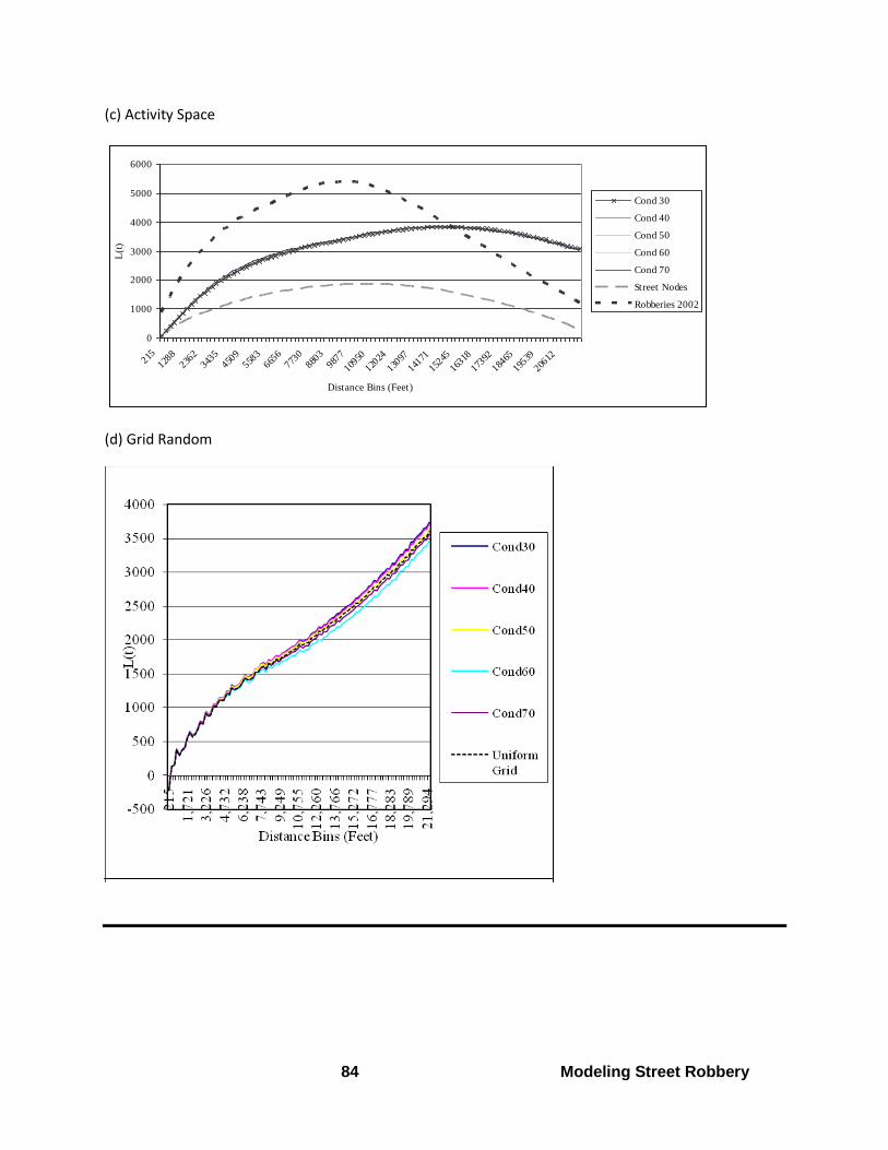
84 Modeling Street Robbery
(c) Activity Space
0
1000
2000
3000
4000
5000
6000
215
1288
2362
3435
4509
5583
6656
7730
8803
9877
10950
12024
13097
14171
15245
16318
17392
18465
19539
20612
Distance Bins (Feet)
L(t
)
Cond 30
Cond 40
Cond 50
Cond 60
Cond 70
Street Nodes
Robberies 2002
(d) Grid Random

85 Modeling Street Robbery
An additional analysis of the distribution of visits (i.e. number of times a civilian agent is
at a node) to separate the clustering in street robbery from clustering due to everyday travel
patterns shows that the patterns for visits and robberies are very similar across all model
versions with robberies exhibiting slightly more clustering than would be expected based on the
network. This provides evidence of the existence of additional factors, beyond routine travel,
that are contributing to the greater concentration of street robbery events.31
H4: The temporal and spatio-temporal schedules of civilians while away from home change
the spatial pattern of robbery events.
The second spatial hypothesis (fourth hypothesis overall) explores the impact of
systematically adding temporally and spatially explicit components to the agent behavior on the
spatial distribution of street robberies. Looking back at Table 10, there is significant variation
among the versions and the more time that is spent away from home, the bigger the disparity
among the versions.
Of the versions that use the street network, the Street Random version has the highest
proportions of both, followed by the Temporal version. The Activity Space model has the most
concentrated distribution. Less than 10% of all nodes in Activity Space version ever have a
robbery. In addition, the tabular results highlight the differences between the random version
of the model run on a uniform grid and the same version run on the street network (i.e., Street
Random). A minimum of 94.1% of all nodes have one or more street robberies and that rises to
99.8% by the 70% condition. The percent of places which are repeat victims rises from 79.8% at
31 Due to space constraints the kernel density and Ripley’s K results for the analysis of visits are not

86 Modeling Street Robbery
the 30% condition to 98.8% at the 70% condition. That means that the Uniform Random model
has almost universal repeat victimization of places which the model versions based on the
street network range only from a low of 7.1% for the Activity Space to a high of 84.6% for the
Street Random version (at 70%).
Kernel density maps (Figures 7, 8, and 9 shown earlier) reveal the existence of intra-
version and inter-version differences in the spatial patterns of street robbery that persist from
the as time spent away from home increases. In general, the Simple condition has fewer
clusters then the Temporal version but the clusters represent higher density areas, regardless
of the experimental condition (Figures 7 and 8). The location of the densest clusters are in the
same general area (e.g. in and near the downtown) for both versions but the distribution for
the rest of the city is very different. The Simple model has more clusters in the southern part of
the city and the Temporal Activity Space has more in northern Seattle. As the only spatially-
defined version, the Activity Space version has a pattern distinctly different from the other
versions; one that reflects the unchanging activity spaces of the agents in the model. At the
opposite end of the spectrum, the Uniform Grid outcome pattern is very different from the
other three versions (Figure 9).
Kernel density maps confirm that street robberies are more dispersed under the Grid
Random version than the Street Random version and that the spatial pattern to a large extent
reflects the underlying street pattern (Figures 7 and 8). Where the street network is denser,
the likelihood of people converging and a crime happening is higher. The Grid Random pattern
included in the paper but are available upon request from the author.

87 Modeling Street Robbery
is in stark contrast to other versions and the drastic shift in spatial pattern shows the
importance of the street network in structuring human activity (Figure 9).
There are also significant differences in the spatial pattern of street robberies between the
three street-based versions. The Street Directed version of the model produces more clustered
crime patterns. Much smaller proportions of nodes have a single robbery (9 versus 83 percent)
or multiple robberies (7 versus 79 percent) in the Street Directed version versus the Street
Random version (Table 6). Once again, the kernel density maps confirm the change in the
pattern of clustering between versions. The pattern from the Street Directed version is
extremely clustered along high volume pathways that represent areas of greatest routine
activity. Both the changes in incidence and pattern revealed by the results are in line with
empirical findings related to the characteristics of crime patterns.
Previous research has clearly established that crime is clustered rather than dispersed in
space (Manson, 2001). Violent crime tends to be even more concentrated in even fewer areas.
These empirical patterns reflect the uneven distributions of opportunities for transportation,
housing, recreation, and employment. Given the above findings, the outcome of the Street
Directed version of the model most closely matches we would expect based on empirical data.
The other versions also produce plausible results. That is we would expect random movement
on a uniform grid to produce a more dispersed pattern of crime than random movement on a
street network just by virtue of varying densities of streets in different parts of the city. Finally,
a landscape that clusters opportunities and structures human activity on a street network
would be expected to produce the most clustered and thus most realistic pattern of street

88 Modeling Street Robbery
robbery events. Thus the results of the model confirm the importance of ‘situating’ simulation
when modeling crime events.
Another way to examine the differences in the spatial pattern of street robberies
produced by the addition of time and then time-space to the civilian’s activities is to use the
Ripley’s K calculated earlier but compare the distributions produced by the model versions at
the 30 and the 70 percent experimental conditions (Figure 11).32 The street robbery pattern
produced by the Activity Space version is significantly more clustered than under the Street
Random (Simple) or Temporal version than would be expected based on the street node
network regardless of experimental condition. This result is reasonable because the Activity
Space version specifically restricts civilians to pre-defined activity spaces for the duration of the
model run.
32 Only the 30 and 70 percent graphs are included in the paper. Results from the 40, 50, and 60 percent conditions are available from the author.

89 Modeling Street Robbery
Figure 11: Ripley’s K Analysis: Distribution of Street Robberies by Model Version
(a) Condition 30: Society Spends 30 Percent of Time Away From Home
(b) Condition 70: Society Spends 70 Percent of Time Away From Home

90 Modeling Street Robbery
On the other hand, the pattern of clustering in the Street Random (Simple) and
Temporal versions relative to one another changes depending on time spent away from home
(Figure 11a and 11b). Although both are more clustered then the street nodes at distances
under two miles, the strength of that clustering varies with experimental condition. The Street
Random (Simple) version exhibits higher levels of clustering at distances under two miles for 30
percent condition. At 70 percent the results are identical at shorter distances but after about a
mile they two versions switch roles and the Temporal version exhibits greater clustering
because of the smaller activity spaces. Overall, temporal constraints reduce clustering in the
distribution at distances between one-half and two miles but only in societies in which civilians
spend up to half of their time away from home. In sum, adding spatial constraints produces a
much larger effect than adding temporal ones.
Evaluation of the Grid Random version offers additional information. The pattern of
robberies in the Grid Random version is essentially identical under both regardless of the time
spent away from home (Figure 11). The only thing that changes is the intensity of crime. This
result reinforces the role of the street network in shaping the pattern of robberies.
Sensitivity Test Results
Sensitivity testing is essential to quantifying the robustness of the model results and is
conducted by varying the initial parameters and the random number seed (2006). The values of
five of the parameters (i.e. number of police, time to wait before able to re-offend, initial
wealth distribution, perception of target suitability random term and the perception of
guardianship random term) are increased; the model runs repeated for all five experimental
conditions; and a one-way ANOVA applied to analyze the results. While the absolute number of

91 Modeling Street Robbery
street robberies increased or decreased depending on the parameter being varied, in all cases
the original significant differences between the groups remained, demonstrating the
robustness of model results to changes in initial parameters. Finally, the entire sensitivity
testing process of varying the five parameter values is repeated four more times using different
random number seeds to test the effect of changing the random number seed on the outcomes
of the model.
An analysis of the output demonstrates that model results are robust to changes in the
random number seed.33 All of the model versions are robust to changes in parameters and
random number seeds. The absolute number of robberies increased or decreased depending
on the parameter being varied. However, between group differences remain consistent across
all the tests (i.e. differences in Temporal are significant and those in Activity Space are not
except for one, see below) lending additional support for robustness of the model even as
parameters are varied. One of tests varying the random number seed did produce a significant
result for the Activity Space version which is the only difference from the base model results.
Otherwise, the results of the model were shown to be robust to changes in the random number
seed.34
Summary of Findings
Three major findings emerge from these efforts. First, support for routine activity theory’s
core proposition depends on the type of schedule constraints placed on the agents. When
33 The results of the sensitivity tests with random number seeds of 200, 300, 400 and 500 are available upon request.

92 Modeling Street Robbery
agents have no constraints on their travel or when they have only temporal constraints (i.e. the
Uniform Random or Street Random and Temporal versions), the number of street robberies
increases as the agents spend more time away from home. However, when the agents are
assigned spatio-temporally defined activity spaces, the incidence of street robbery still
increases but the differences among the experimental conditions are not statistically
significant. Therefore, the findings provide support for routine activity theory’s core
proposition but not when the agent’s activity spaces are spatially constrained. This finding also
provides evidence of the importance of the spatial component of routine activity in structuring
where and with whom convergences occur.
The finding of non significance for the Activity Space version has theoretical implications. It
demonstrates that spatial constraints counteract the influence of increasing time spent away
from home. Not completely, since crime continues to increase with time spent away from
home in the Activity Space version. However, enough to reduce the differences between the
experimental conditions and render them non significant. Thus it is the spatio-temporal
etiology of routine activity, and not just the gross amount of time spent away from home, that
underpins macro level robbery rates.
The implementation of activity spaces in the model is one potential source of explanation
for the lack of significant findings for the Activity Space version. The maximum of two only
potential activity spaces (i.e. when employed and when unemployed) constrains the spatial
extent of agent travel to an unrealistic degree. Consequently, during any model run specific
34 All numeric results are available upon request from the author.

93 Modeling Street Robbery
agents can only converge with the relatively few other agents whose activity spaces intersect
their own. While activity spaces are somewhat static, it is the degree to which activity spaces
are constrained that is the issue. In the model, the repeated interaction of the same agents
quickly causes the offender agents to gain more wealth than the civilian agents, so that no
crime occurs when only two civilians converge and the offender has more wealth. As a result,
increasing convergences do not translate into higher numbers of robbery. While this
phenomenon is present in all three versions of the model, it is most pronounced in the Activity
Space version. Figure 12 shows the precipitous drop in daily robbery statistics for all three
versions. Three potential strategies that may ameliorate this phenomenon are to: 1) make the
wealth distribution for citizens reflect criminal propensity by assigning offenders lower wealth;
2) increase the number of civilian agent activity spaces available for agents; and 3) boost the
number of civilian agents in the model.
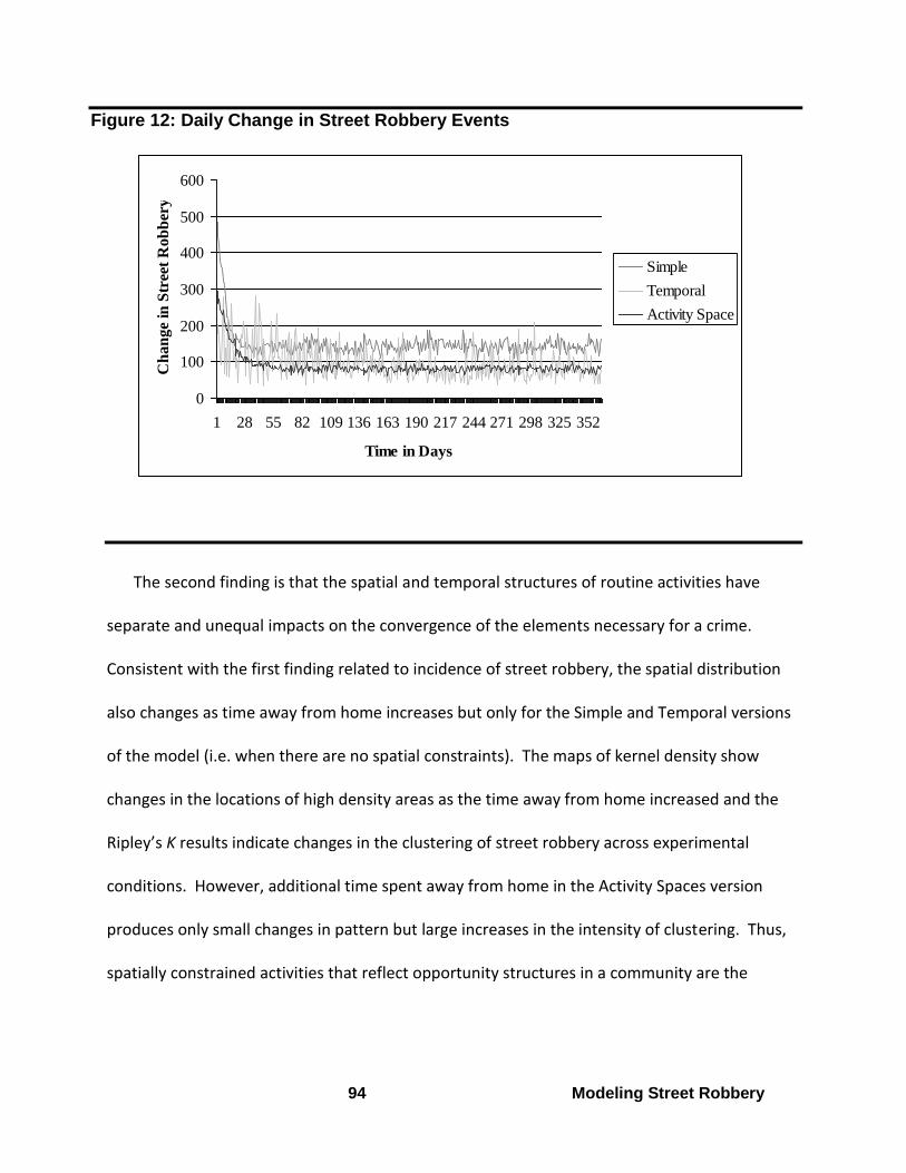
94 Modeling Street Robbery
Figure 12: Daily Change in Street Robbery Events
0
100
200
300
400
500
600
1 28 55 82 109 136 163 190 217 244 271 298 325 352
Time in Days
Ch
an
ge
in S
tree
t R
ob
ber
y
Simple
Temporal
Activity Space
The second finding is that the spatial and temporal structures of routine activities have
separate and unequal impacts on the convergence of the elements necessary for a crime.
Consistent with the first finding related to incidence of street robbery, the spatial distribution
also changes as time away from home increases but only for the Simple and Temporal versions
of the model (i.e. when there are no spatial constraints). The maps of kernel density show
changes in the locations of high density areas as the time away from home increased and the
Ripley’s K results indicate changes in the clustering of street robbery across experimental
conditions. However, additional time spent away from home in the Activity Spaces version
produces only small changes in pattern but large increases in the intensity of clustering. Thus,
spatially constrained activities that reflect opportunity structures in a community are the

95 Modeling Street Robbery
source of generally stable hotspots that increase in intensity as time spent away from home
increases.
Thirdly, temporal and spatio-temporal constraints have a differential influence on the
incidence of street robbery. As compared to the Simple version, in which agents are either at
home or not at home, the addition of temporal schedules for civilian agents reduces the
incidence of street robbery by about 77% and changes the distribution of street robbery events.
This result provides evidence in support of Ratcliffe’s (Miller, 1991) hypothesis that temporal
constraints are a major source of observed patterns of opportunity-based crime. When spatially
defined activity spaces are added to the model and the temporal schedule for each agent is
held constant, the separate and even larger impact of space is clearly demonstrated. Spatio-
temporally constrained schedules significantly increase the incidence of street robbery as
compared to agents with a temporal schedule only and radically change the distribution of
street robbery events. The clustering in the spatial distribution of robberies is higher than the
other versions and more linear in nature due to concentration along the major travel routes
among homes, jobs and activities.
Fourthly, the street network is of critical importance in shaping the spatial pattern of street
robberies. While the total number of street robberies under Grid Random and Street Random
were not significantly different, the spatial pattern varied considerably. The pattern of Street
Random robberies exhibits clustering which is a characteristic of empirical street robbery
patterns. Thus, in two models with exactly the same agent behavior but different landscapes,
the only possible explanation for the difference in pattern is the street network.

96 Modeling Street Robbery
These findings regarding differences by type of schedule constraints are consistent across
all five experimental conditions. In other words, regardless of time spent away from home, the
type of schedule (i.e. simple, temporal or spatio-temporal) produces significantly different
numbers and patterns of street robbery. Thus, the impact of temporal and spatio-temporal
constraints on activity is robust with regard to time spent away from home.
There are several potential explanations for these findings that originate from the
construction of the model and the experiments. The changes in incidence and pattern could be
related to the amount of time the agents are ‘at risk’. The addition of a temporal schedule
reduces both the time that civilian agents are ‘at risk’ of being victimized and the time that
civilians with criminal propensity have to offend. In this way, temporal schedules constrain the
activities of both offenders and non-offenders and directly influence the number and pattern of
convergences. Differences in time ‘at risk’ do not explain the increase in street robberies
between the Temporal and Activity Space versions because the temporal schedule is held
constant between the two.
The explanation for differences between the Temporal and Activity Space versions of the
model lies in the clustered nature of human activity that is reflected in the Activity Space
version of the model. The homes of civilian agents are concentrated in certain areas, they
travel to jobs that are clustered in other areas and they participate in activities that have yet
another, but still clustered, distribution. The road network acts to amplify this result in that
agents traveling to the same area tend to be routed along the same major roads. In this way,
the implementation of spatio-temporal routine activity spaces following time geographic

97 Modeling Street Robbery
principles acts to increase overlap in activity spaces which in turn, increases the frequency of
convergence. One interesting side effect of this increased concentration is that police agents
who are randomly assigned to patrol in those high concentration areas are able to deter more
crimes than when civilian agents are only temporally constrained but randomly distributed (as
in the Temporal version of the model). This finding has implications for achieving a better
understanding the relationship between police patrol strategies and crime.
Explanations for the Emergent Patterns
Explanations for the findings just described have their roots in the simple rules
governing agent behavior and interaction. The separate influences of temporal and spatio-
temporal schedules and the movement rules of the agents underlie the finding that time and
space each have an effect on the incidence and spatial distribution of street robbery events
stems. Temporal schedules reduce the time agents are ‘at risk’. Agents with a temporal
schedule spend time at their activity nodes which means they are not vulnerable to street
robbery for as much time and they travel shorter distances each day. These changes to their
behavior directly impact the number of times they end up at a place where a crime might occur
(i.e. the number of convergences) and thus, the rate of street robbery in society. They also
change the spatial distribution of robbery events by making the potential path space of the
agents in the Temporal version smaller.
Adding a spatially-defined activity space to temporally-defined agents yields a version of
the model in which the civilians have the same time ‘at risk’ compared to agents in the
Temporal version but travel among a set of places that reflect the distribution of homes, jobs

98 Modeling Street Robbery
and activities in Seattle. Empirically-informed spatio-temporal activity spaces in the Activity
Space version of the model increase convergences in two ways. First, they increase the
clustering of homes, jobs and activity nodes as compared to a random distribution. As a result,
civilians are funneled along many of the same roads to reach many of the same areas. Second,
the use of a defined activity space embodies the routine nature of daily travel and its restriction
to a potential path area in which individuals can travel to all the required locations within their
time schedule (Kwan, 1998; Weber & Kwan, 2002). Civilians following these predefined paths
are by definition then going to converge only with other civilians’ paths that physically
intersect. In this way, spatially-defined activity spaces act to: 1) concentrate the activities of
agents sharing the same activity space; and 2) increase the frequency of convergence of agents
in the model; and 3) increase the deterrence effect of police who are in those high
concentration areas.
Adding a spatially-defined activity space produced results that did not support RAT’s
premise that as time spent away from home increases, crime will increase. The explanation for
this finding is probably in the implementation of the model rather than the theory itself.
Currently, the activity spaces of civilians are unrealistically consistent which concentrates their
interaction to one daily path. While this type of activity space may be accurate for some small
proportion of individuals, accessibility research indicates there is typically more variety in daily
paths (Bureau of Labor Statistics, 2003). As a consequence of this concentrated interaction in
the model, the same civilians with and without criminal propensity meet again and again. As
the civilians with criminal propensity accumulate more wealth than the non-criminal civilians,
especially in situations where there are only two agents (criminal and non-criminal civilian), no

99 Modeling Street Robbery
crime will occur. Thus while the frequency of convergence in the model continues to increase
dramatically, the rise in street robberies is much slower and there are not significant
differences as society spends more time away from home.
Increasing the variety of agent paths or increasing the number of agents in the
population might produce a finding consistent with routine activity theory but was not part of
the original work done here.
Extending the Model
Using the initial grant support of NIJ, we developed an additional version of the model
of street robbery, Extended Activity Space version. The Extended Activity Space Model (EAS)
incorporates lessons learned from the shortcomings of the other versions, comment and
suggestions from audiences at professional conferences, and suggestions from peer reviewers.
The EAS attempts to produce crime patterns that are similar to real street robbery events in
Seattle, WA. While the characteristics of the patterns produced by the original Activity Space
version are closest to those of real robberies in Seattle (i.e., they are concentrated in a
relatively few places), the model predicts far too many crime events. Using the feedback
sources mentioned above we made a series of changes to the activity space model to improve
our representation of human behavior. This section discusses those changes in detail and
provides a summary of the results.
A series of five major changes were made to the Activity Space version of the model that
reflected lessons learned from the original three versions. These changes consist of: 1) add
more potential activity spaces for each agent (5 potential activity spaces while employed and

100 Modeling Street Robbery
five while unemployed); 2) tie the wealth of the agent to the block group in which they live; 3)
change the amount of money agents get paid to their initial wealth ranking (low, medium, or
high income); 4) change the amount of money that is taken in a robbery to reflect a percentage
of the victim’s current wealth; 5) have criminality assigned to only low and middle income
agents – high income agents unlikely to look to street robbery for income; and 6) assume car
travel and change the time agents are ‘at risk’ so that agents are not at risk while driving, only
at destination. Each of these changes is explained in the next sections (Table 11).

101 Modeling Street Robbery
Table 11: Comparison of Parameters in the Original and Extended Versions
Variable Rationale
Society Level
All models
Number of Agents = 1,000
Represents a balance between ensuring there are enough agents so
that interactions can occur and the computational overhead from
using more agents
Number of Cops = 200
Chosen to ensure that cops would be present at some of the
convergences that occur across the 16,035 places in Seattle.
Unemployment Rate = 6%
The unemployment rate of six percent is based on the 2002
unemployment rate for Seattle (Visher & Roth, 1986).35
Rate of Criminal Propensity =
20%
Given that 20% of the population has committed a crime, 20% of
civilians are assigned criminal propensity using a uniform distribution
(Ropella et al., 2002).
Time To ReOffend = 60
Parameter value chosen as a starting point since the author could find
no empirical data on which to base time to reoffend..
Random Number Seed = 100
(seed also tested at 200,
300, 400 and 500)
An explicit random number seed based on the Mersenne Twister
(MT) algorithm is used as the basis for all random number
distributions used in the model. MT is currently considered to be the
most robust in the industry (Reppetto, 1976).
Agent Level
Original Extended
Societal Time Spent Away
From Home = 30% (40%,
50%, 60%, 70%)
Assigned based on a normal distribution with a mean of 432 minutes
(for the 30% condition) and a standard deviation of 10% of the mean
(sd = 43).36
35 Since the jobs data are from 2002, the corresponding year’s unemployment rate is used.
36The time spent away from home is systematically varied to test the core proposition of routine activity that as time spent away from home increases crime will increase.

102 Modeling Street Robbery
Initial
Wealth = 50
Initial
Wealth
varies by
home block
group
Initial wealth is assigned with a
mean of 50 and a standard
deviation of 20 units.
Initial wealth assigned by class:
Low - 0 – $34,999
Med -$35,000 to $64,999
High -$64,999 and up
Wealth
received
each payday
= 5
Wealth
received
each payday
proportional
No empirical evidence available. Wealth received each payday
proportional to beginning wealth
Wealth
exchanged
during
robbery = 1
Wealth
exchanged
during
robbery
varies
No empirical evidence
available.37
Wealth exchanged during
robbery 10% of victim’s current
wealth
Situation Level
Original Extended
Guardianship
Perception =
U(-2,2)
Guardianship
Perception =
U(-4,4)
The guardianship perception
value can add or subtract zero,
one or two guardians from the
actual number present. This
represents the stochastic
element in the offender’s
perception of the level of
guardianship present.
The guardianship perception
value can add or subtract zero,
one, two, three, or four
guardians from the actual
number present. This represents
the stochastic element in the
offender’s perception of the level
of guardianship present.
Suitable
Target
Perception =
U(-1,1)
Suitable
Target
Perception =
U(-
1,000,1,000)
The value in suitable target can increase or decrease the suitability or
leave it unchanged. This enables the offender to sometimes decide a
target is not suitable even when they have more wealth.
37 A request to the Seattle Police Department for the average amount of cash taken during street robberies remains unanswered.
103 Modeling Street Robbery
The most important change was to add more potential activity spaces and thereby increase
the potential size and change the shape of agent activity in the model. To get five different
paths for each agent when employed and when unemployed, 15,000 nodes instead of the 3,000
nodes that were selected for the original model were proportionately selected. Those nodes
were then randomly allocated to the agent’s five different potential activity spaces. The
program to find the shortest path among the locations was updated and applied to the new
activity spaces. The lists of nodes were loaded into the agent objects in Agent Analyst and the
Agent Analyst code was changed to allow each agent to randomly select a set of locations to
visit in that day. So instead of each civilian agent having only two (Activity Space version) , they
now have a have a total of ten potential activity spaces that are randomly selected each day
based on employment status. Employed and unemployed activity spaces remain identical
except that the work location is dropped from the unemployed path and a new activity location
is added.
The second major change was to tie the income levels of agents to the area in which
they reside. This enabled the agent ‘society’ to more closely mirror the empirical distribution of
wealth in Seattle. Block groups were assigned to be high, medium or low income using the
actual income categories from the 2000 census.38 Agents assigned to live in a block group were
also assigned a wealth from the distribution for that neighborhood. For example, an agent
38 Low income neighborhoods ranged from 0 – 34,999 (18.6% of all block groups, mean = $18,594, SD = $3,951), medium income neighborhoods ranged from $35,000 to $64,999 (57.5% of all block groups, mean = $48,098, SD $3,661) and high income neighborhoods consisted of $64,999 and up (23.9% of all block groups, mean = $119,776, SD = $8,263).

104 Modeling Street Robbery
from a low income neighborhood was assigned a wealth amount from a normal distribution
with a mean of $18,594 and a standard deviation of $3,951.
Pay was changed so that it reflected the beginning income level of the agent. So an
agent with a $30,000 annual income would be paid half as much as an agent making $60,000
during the model run. Unemployed agents are not paid. This enhancement was also intended
reflect the geographical distribution of ‘suitable targets’/opportunities for street robbery.
Related to the changes in income and pay, the assignment of criminality was limited to
only those agents who resided in low and middle income neighborhoods – high income
neighborhood residents were considered unlikely to look to street robbery for income. In
addition, the amount of money taken in a robbery was changed from a static amount to reflect
a percentage of the victim’s current wealth.
Another enhancement was to change the risk status to be more realistic. The EAS
version assumes the primary mode of transportation to be personal automobile but now allows
for the fact that many people park their cars and walk one to four blocks. In the enhanced
model, agents within one to four nodes (the actual number is randomly selected each time)
change their travel speed and their risk status to reflect the change from automobile travel to
walking (i.e., they slow down and become ‘at risk’ of committing or being a victim of a street
robbery). In a related change, unemployed agents are ‘at risk’ at their main mode since the
model no longer assumes they are inside a building.
Together these changes represented a comprehensive upgrade of the model. We then
tested the outcomes to see how well the new model version did.
105 Modeling Street Robbery
Findings from the Enhanced Model Version
The purpose of the enhanced model version was to discover whether the model could
be used for policy exploration specifically testing the effects of different policing strategies. In
order for the model to used for such policy exploration it needed to produce results that were
clustered in space at roughly the same magnitude as street robberies occurred in Seattle. Since
the main goal of this exploration was to find out if the model could meet the two criteria just
stated, the testing of this model varied from the experimental conditions of the other models.
Testing was begun at the 30% experimental condition and only if the numbers were plausible
would the testing proceed to the other conditions.
So beginning with the 30% condition and holding all but the enumerated changes constant
the Extend Activity Space version of the model produced fewer robberies (n = 19,457) than the
Activity Space version (n = 32,326). Unfortunately, the actual number of street robberies in
Seattle is 1,156. While the changes to the program increased its representational validity, they
did not decrease the number of street robberies to anywhere close to the ‘real’ rate. In
addition, they did not result in a ‘spread’ of hot spot areas beyond the downtown (Figure 13).
Together, the inability to generate a similar pattern or rate of street robbery mean that the
model cannot be validated and thus is of debatable suitability for further use as a tool for
evaluating the policy implications of changes to patrol etc. Further work is needed on the
model before it is ready for those sorts of applications.

106 Modeling Street Robbery
Figure 13: Comparison of Kernel Density for Activity Space (cond=30) and Extended Activity Space (cond=30)

107 Modeling Street Robbery
Implications for Policy and Practice This demonstration of modeling criminal behavior at the individual level provides an
alternative method for exploring the basic assumptions of routine activity theory. Previous
attempts to operationalize the theoretical constructs have been hampered by a lack of data
about individual’s routine activities and other situational characteristics and the lack of tools
capable of modeling individual interactions across space and time. Consequently, they have
provided mixed evidence of the veracity of routine activity theory. This research is able to
model the basic components of routine activity theory through the use of agent-based
modeling. In an agent-based model, single aspects of the behaviors of agents can be
manipulated while all others are held constant. In addition, the landscape can be held constant
across models. This research focus implemented only an initial model and represents only a
‘bare-bones’ version of what could be done in future simulations.
Although the model is simple, its implementation accomplishes several essential
functions. First, this effort establishes a foundation for further, more complex explorations of
criminal behavior. The agents and police officers developed for this research have the core
behaviors that are essential to the creation of richer representations of behavior. Second, the
software used for model development is open source, the code for the street model is provided
as is documentation. Tothether these provide a transparency to the model that is rarely found
and which should facilitate the work of future researchers who wish to replicate the results or
build on this effort. Third, the theoretical aspects of routine activities are multi-layered. This
model implements the coarsest level. Subsequent models will incorporate finer details using

108 Modeling Street Robbery
this model as a platform. Fourth, the model offers a set of results that can be evaluated and
discussed to determine necessary changes and serve as a starting point for further research. In
this way the model acts as a ‘straw man’ which will stimulate discussion about changes and
enhancements. Finally and maybe most importantly in the long run, the model demonstrates
how we can explore the impact of human behavior in an artificial environment to better
understand the formation of crime patterns. As models become more accurate, they will
provide forums for exploring the impact of policy decisions.39 This is particularly important in
the social sciences when policy makers must often choose between competing strategies.
While this model is not be ready for prediction, it demonstrates the potential of agent
based modeling. With additional work on the parameters and the analytical capability of this
base model we could potentially examine a variety of policy questions related to crime
prevention, policing strategies, and response to terrorist incidents. Computational laboratories
can be used to test the veracity of theoretical assumptions in advance of empirical research.
This strategy has the potential to be far more cost-effective because new policies can be
‘tested’ within the simulation and only those that show promise funded for field research.
In the area of crime prevention, policies suggested by Crime Prevention through
Environmental Design (CPTED) and opportunity theories can be studied intensively. The
physical design and access control strategies suggested by CPTED are often very expensive
(Gottfredson & Hirschi, 1990). Simulation saves money by helping to identify the strategies
39 We are indebted to the anonymous NIJ reviewers in the spring of 2004 for suggesting we emphasize the utility of computational laboratories for evaluation of policy choices.

109 Modeling Street Robbery
with the highest potential for success on the ground. The quantitative output of the
simulations can be used in preliminary cost-benefit analyses to evaluate new methods.
Opportunity theories have hypothesized about the elements necessary for a crime to
occur as well as the physical and social environment. In a computational laboratory each one of
these components can be analyzed while the others are held constant.40
In this way the often confounding effects of variables can be separated. For instance,
the decision to offend can be studied intensively. Instead of having criminal propensity as a
presence/absence trait, criminality could be assigned randomly and in various strengths.
Criminal tendency could then be used as a variable in a more complex equation describing the
decision to offend in a particular situation.
Agents could ‘learn’ from the relative success of previous decisions and use that
information in future decisions. For instance, agents could have the ability to ‘recognize’ other
agents with whom they come in contact at a node. Each time two agents come in contact with
one another the concurrence could be stored for future reference. This information would be
called upon when an agent is making the decision to offend. Social control theory (Eck, 1995a)
postulates that if the agent ‘knows’ another agent at the scene, the probability that the agent
will commit the crime is reduced because of informal social control. The possibility of being
recognized probably also has an effect. Disaggregating the factors involved in the decision to
40 The other components are not actually held constant but rather the same random number algorithm is used for each experiment so that each run is the ‘same’ as the last. Thus we can be sure that any change in the outcome is due to the purposeful change being made and not due to other, unknown factors.

110 Modeling Street Robbery
offend is necessary to gain a better understanding of each individual factor and how they
interact.
Another important facet of opportunity is the issue of guardianship. Questions
concerning the role of place managers (Felson, 1986) and intimate handlers (P. Brantingham &
P. Brantingham, 1981b, 1981c; P. J. Brantingham & Brantingham, 1984; P. L. Brantingham &
Brantingham, 1993) as guardians could be tested in a computational laboratory. In fact, the
entire phenomena of guardianship could be dissected in such a laboratory because of the
ability to hold factors constant. A researcher could change the weightings of agents
representing guardianship (e.g. police officers, known agents, place managers, etc.) to
determine the effect on the decision to offend.
In addition to examining the agents’ interactions with one another, their interaction
with the environment could also be studied. One intriguing aspect is to study the effect of
urban form on the physical configuration of routine activities undertaken by the agents.
Theory holds that criminals, as well as other individuals, become familiar with areas and their
associated opportunities for crime via the travel routes they use in their own routine activities
(E. Groff, 2008; E. Groff & Birks, 2008; E. R. Groff, 2007a, 2007b, 2008a, 2008b). This
assumption could be tested in a computational laboratory. Another area of research concerns
the journey to crime. A computational laboratory enables agents to be assigned behavioral
rules and then allow patterns of behavior to emerge. In this way, research could allow the
comfort zone of an offender to emerge from the simulation. Comparing the functional

111 Modeling Street Robbery
distributions from the simulations with those from empirical research could test the veracity of
the patterns observed.
Related to police patrol strategies, the distribution of agents and/or police officers
across the landscape could be changed and the effect on macro-level crime patterns observed.
For example, a simple experiment that changes the initial geographic distribution of agents
(e.g., random vs. clustered vs. uniform) would provide interesting information about the effect
of changes in population distribution on emerging crime patterns. These types of models could
be also be used to test the effectiveness of different patrol patterns on crime reduction (e.g.,
hot spot policing). For example, a researcher could use the results of the previous simulation
(and the same random number seed) to assign police officers to small areas with high crime and
see how the pattern/rate of crime changes. Spatial statistics could be used to compare
resulting patterns and more rigorously test the significance of the results. The optimum
number of police officers for a particular jurisdiction could be explored by comparing the crime
levels at varying force sizes.41 Diffusion is another area related to police effectiveness that
could be examined in new depth with computational laboratories.
In an agent-based model we are not limited to comparing only individuals or society,
analysis can be done at the level of neighborhood or place. In addition, the modeling itself
could be done at the neighborhood level and the impact of neighborhood changes in
41 We are indebted to the anonymous reviewer for suggesting that experiments could be conducted to find the optimal ratio of police officers to citizens using simulation.

112 Modeling Street Robbery
demographics, socioeconomics, and physical characteristics could be tested for their effect on
citywide patterns.
The potential of the computational laboratory for theoretical testing and exploration is
is just beginning to be explored. As described earlier, as the first attempt to test routine activity
theory within an agent based computational laboratory this effort provides a foundation for
additional, more accurately and richly specified models to be developed. These advanced
models have the potential to produce concrete, public policy relevant findings to address the
situational elements of crime since opportunity theories by definition concentrate on aspects of
the crime event that can be changed far more quickly and easily than ones involving the root
causes of criminal motivation.
Dissemination of Methodology and Findings We have attempted to publicize and make available both the methodology and the
custom models available to a wide variety of researchers to facilitate the adoption of the
methodology. This research relies on commercial software, ArcGIS, SPSS and Excel as well as a
free, open source software extension to ArcGIS, Agent Analyst, to create a computational
laboratory and analyze the results. All software code is part of Appendices 1-3 that contain the
documentation of the model. Digital versions of the code are also being delivered on a DVD.
Anyone can download Agent Analyst software from
http://www.institute.redlands.edu/agentanalyst/AgentAnalyst.html.
The findings from this work were presented at the American Society of Criminology (to
reach the academic community) and the Academy of Criminal Justice Sciences (to reach

113 Modeling Street Robbery
practitioners). There have been a total of six publications from the research activities funded
by NIJ (E. Groff, 2008; E. R. Groff, 2007a, 2007b, 2008a, 2008b). One of these lays out the use
of simulation to explore theory (E. R. Groff, 2007a), another discusses the technical aspects of
achieving agent travel on a realistic vector network (E. R. Groff, 2007b), two other report results
from models (E. R. Groff, 2008a, 2008b), and the final two discuss potential applications to
inform policy (E. Groff, 2008; E. Groff & Birks, 2008). ESRI will be publishing a book about using
Agent Analyst software and two chapters will be directly related to this research.
114 Modeling Street Robbery
References Aitken, S. C., Cutter, S. L., Foote, K. E., & Sell, J. L. (1989). Environmental Perception and
Behavioral Geography. In Wilmott & Gaile (Eds.), Geography in America (pp. 218-238).
Akers, R. L. (2000). Criminological Theories: Introduction, Evaluation, and Application. Los
Angeles: Roxbury Publishing Company.
Axelrod, R. (2006). Simulation in the Social Sciences. In J.-P. Rennard (Ed.), Handbook of
Research on Nature-Inspired Computing for Economy and Management (Vol. 1, pp. 90-
100). Hershey, PA: Idea Group.
Axelrod, R. (Forthcoming). Advancing the Art of Simulation in the Social Sciences. In J.-P.
Rennard (Ed.), Handbook of Research on Nature Inspired Computing for Economy and
Management. Hershey, PA: Idea Group.
Bailey, T. C., & Gatrell, A. C. (1995). Interactive Spatial Data Analysis. Essex: Longman Group
Limited.
Batty, M., & Torrens, P. M. (2005). Modelling and Prediction in a Complex World. Futures, 37,
745-766.
Beccaria, C. (1963). On Crimes and Punishments (H. Paolucci, Trans.). Upper Saddle River:
Prentice-Hall.
Birks, D., Donkin, S., & Wellsmith, M. (2008). Synthesis over Analysis: Towards an Ontology
for Volume Crime Simulation. In J. Eck & L. Liu (Eds.), Artificial Crime Analysis
Systems: Using Computer Simulations and Geographic Information Systems (pp. 160-
192). Hershey, PA: Idea Group.
Boruch, R. F. (1997). Randomized Experiments for Planning and Evaluation. Thousand Oaks,
CA: Sage Publications.
Brantingham, P., & Brantingham, P. (1981a). Environmental Criminology. Prospect Heights, IL:
Waveland Press, Inc.
Brantingham, P., & Brantingham, P. (1981b). Introduction to the 1991 Reissue: Notes on
Environmental Criminology. In P. Brantingham & P. Brantingham (Eds.), Environmental
Criminology (pp. 1-6). Prospect Heights: Waveland Press Inc.
Brantingham, P., & Brantingham, P. (1981c). Notes on the Geometry of Crime. In P.
Brantingham & P. Brantingham (Eds.), Environmental Criminology (pp. 27-54). Prospect
Heights, IL: Waveland Press, Inc.
Brantingham, P. J., & Brantingham, P. L. (1981). Notes on the Geometry of Crime. In P.
Brantingham & P. Brantingham (Eds.), Environmental Criminology (pp. 27-54). Prospect
Heights, IL: Waveland Press, Inc.
Brantingham, P. J., & Brantingham, P. L. (1984). Patterns in crime. New York Macmillan.
Brantingham, P. J., & Brantingham, P. L. (1991). Introduction to the 1991 Reissue: Notes on
Environmental Criminology. In P. Brantingham & P. Brantingham (Eds.), Environmental
Criminology (pp. 1-6). Prospect Heights: Waveland Press Inc.
Brantingham, P. L., & Brantingham, P. J. (1993). Nodes, Paths and Edges: Considerations on
the Complexity of Crime and the Physical Environment. Journal of Environmental
Psychology, 13, 3-28.
Brantingham, P. L., & Brantingham, P. J. (2004). Computer Simulation as a Tool for
Environmental Criminologists. Security Journal, 17(1), 21-30.

115 Modeling Street Robbery
Brantingham, P. L., & Groff, E. R. (2004). The Future of Agent-Based Simulation in
Environmental Criminology. Paper presented at the American Society of Criminology,
Nashville, TN.
Brown, D. G., Riolo, R., Robinson, D. T., North, M., & Rand, W. (2005). Spatial Process and
Data Models: Toward Integration of Agent-Based Models and GIS. Journal of
Geographic Systems, 7, 25-47.
Bureau of Labor Statistics. (2003). Metropolitan Area Employment and Unemployment:
January 2003. 2006, from www.bls.gov/news.release/archives/metro_03262003.pdf
Bursik, R. J. J., & Grasmick, H. G. (1993). Neighborhoods and Crime: The Dimensions of
Effective Community Control. New York, NY Lexington Books.
Calthrope, P. (1993). The Next American Metropolis: Ecology, Community and the American
Dream. New York: Princeton Architectural Press.
Chorley, R. J., & Haggett, P. (Eds.). (1967). Models in Geography. London: Methuen & Co.
Clarke, R. V., & Cornish, D. B. (1985). Modeling Offender's Decisions: A Framework for
Research and Policy. In M. Tonry & N. Morris (Eds.), Crime and Justice: An Annual
Review of Research, Volume 6. Chicago: University of Chicago Press.
Cohen, L. E. (1981). Modeling Crime Trends: A Criminal Opportunity Perspective. Journal of
Research in Crime and Delinquency, 18, 138-163.
Cohen, L. E., & Felson, M. (1979). Social Change and Crime Rate Trends: A Routine Activity
Approach. American Sociological Review, 44, 588-608.
Cohen, L. E., & Felson, M. (1999). Routine Activity Theory. In F. T. Cullen & R. Agnew (Eds.),
Criminological Theory: Past to Present (pp. 258-268). Los Angeles, CA: Roxbury
Publishing Company.
Cohen, L. E., Kluegel, J. R., & Land, K. C. (1981). Social Inequality and Predatory Criminal
Victimization: An Exposition and Test of a Formal Theory. American Sociological
Review, 46, 505-524.
Cornish, D. B., & Clarke, R. V. (1986). Introduction. In D. B. Cornish & R. V. Clarke (Eds.),
The Reasoning Criminal: Rational Choice Perspectives on Offending (pp. 1-13). New
York: Springer-Verlag.
Cullen, F. T., & Agnew, R. (Eds.). (1999). Criminological Theory: Past to Present. Los
Angeles, CA: Roxbury Publishing Company.
Dibble, C. (2003). Theory in a Complex World: GeoGraph Computational Laboratories.
submitted Nystrom 2003.
Dibble, C. (2006). Computational Laboratories for Spatial Agent-Based Models. In L. Tesfatsion
& K. L. Judd (Eds.), Handbook of Computational Economics, Vol 2: Agent-Based
Computational Economics (Vol. 2). Amsterdam: Elsevier.
Dowling, D. (1999). Experimenting on Theories. Science in Context, 12(2), 261-273.
Duaney, A., & Plater-Zyberk, E. (1993). The Neighborhood, the District and the Corridor. In P.
Katz (Ed.), The New Urbanism: Toward an Architecture of Community. New York:
McGraw-Hill.
Eck, J. E. (1995a). Examining Routine Activity Theory: A Review of Two Books. Justice
Quarterly, 12(4), 783-797.
Eck, J. E. (1995b). A General Model of the Geography of Illicit Retail Marketplaces. In J. E. Eck
& L. Weisburd David (Eds.), Crime and Place (pp. 67-93). Monsey, NY: Willow Tree
Press.

116 Modeling Street Robbery
Eck, J. E. (2005). Using Crime Pattern Simulations to Elaborate Theory. Paper presented at the
American Society of Criminology, Toronto.
Eck, J. E., Gersh, J. S., & Taylor, C. (2000). Finding Crime Hot Spots Through Repeat Address
Mapping. In V. Goldsmith, P. McGuire, G., J. H. Mollenkopf & T. A. Ross (Eds.),
Analyzing Crime Patterns: Frontiers of Practice (pp. 49-64). Thousand Oaks, CA: Sage
Publications.
Eck, J. E., & Liu, L. (2004). Routine Activity Theory in a RA/CA Crime Simulation. Paper
presented at the American Society of Criminology, Nashville, TN.
Eck, J. E., & Liu, L. (2008a). Varieties of Artificial Crime Analysis: Purpose, Structure, and
Evidence in Crime Simulations. In J. E. Eck & L. Liu (Eds.), Artificial Crime Analysis
Systems: Using Computer Simulations and Geographic Information Systems (pp. 413-
432). Hershey, PA: IGI Global.
Eck, J. E., & Liu, L. (Eds.). (2008b). Artificial Crime Analysis Systems: Using Computer
Simulations and Geographic Information Systems. Hershey, PA: IGI Global.
Epstein, J. M., & Axtell, R. (1996). Growing Artificial Societies. Washington DC: Brookings
Institution Press.
Epstein, J. M., Steinbruner, J. D., & Parker, M. T. (2001). Modeling Civil Violence: An Agent-
Based Computational Approach (Working Paper). Washington DC: Center on Social and
Economic Dynamics, Brookings Institution.
Felson, M. (1986). Linking Criminal Choices, Routine Activities, Informal Control, and
Criminal Outcomes. In D. B. Cornish & R. V. Clarke (Eds.), The Reasoning Criminal:
Rational Choice Perspectives on Offending (pp. 119-128). New York: Springer-Verlag.
Felson, M. (1987). Routine Activities and Crime Prevention in the Developing Metropolis.
Criminology, 25(4), 911-931.
Felson, M., & Clarke, R. V. (1998). Opportunity Makes the Thief: Practical Theory for Crime
Prevention (No. 98). London, UK: Home Office, Policing and Reducing Crime Unit.
Gilbert, N., & Terna, P. (1999). How to Build and Use Agent-based Models in Social Science.
Retrieved 9-30-2003, 2003, from http://web.econ.unito.it/terna/deposito/gil_ter.pdf
Gilbert, N., & Troitzsch, K. G. (1999). Simulation for the Social Scientist. Buckingham: Open
University Press.
Gilbert, N., & Troitzsch, K. G. (2005). Simulation for the Social Scientist (Second ed.).
Buckingham: Open University Press.
Gold, J. R. (1980). An Introduction to Behavioural Geography. New York: Oxford University
Press.
Golledge, R. G. (1978). Learning About Urban Environments. In T. Carlstein, D. Parkes & N. J.
Thrift (Eds.), Making Sense of Time (pp. 76-98). New York: John Wiley & Sons.
Golledge, R. G., & Stimson, R. J. (1997). Spatial Behavior: A Geographical Perspective. New
York: Guilford Press.
Golledge, R. G., & Timmermans, H. (1990). Applications of Behavioural Research on Spatial
Problems I: Cognition. Progress in Human Geography, 14, 57-99.
Gottfredson, M., & Hirschi, T. (1990). A General Theory of Crime. Stanford, CA: Stanford
University Press.
Gove, W. R., Hughes, M., & Geerken, M. (1985). Are Uniform Crime Reports a Valid Indicator
of the Index Crimes? An Affirmative Answer with Minor Qualifications. Criminology,
23, 451-501.

117 Modeling Street Robbery
Groff, E. (2008). Simulating Crime to Inform Theory and Practice. In S. Chainey & L. Tompson
(Eds.), Crime Mapping Case Studies: Practice and Research (pp. 133-141): John Wiley
& Sons.
Groff, E., & Birks, D. (2008). Simulating Crime Prevention Strategies: A Look at the
Possibilities. Policing: A Journal of Policy and Practice, 1(0), 1-10.
Groff, E. R. (2007a). Simulation for Theory Testing and Experimentation: An Example Using
Routine Activity Theory and Street Robbery. Journal of Quantitative Criminology, 23(2),
75-103.
Groff, E. R. (2007b). 'Situating' Simulation to Model Human Spatio-Temporal Interactions: An
Example Using Crime Events. Transactions in GIS, 11(4), 507-530.
Groff, E. R. (2008a). Adding the Temporal and Spatial Aspects of Routine Activities: A Further
Test of Routine Activity Theory. Security Journal, 21, 95-116.
Groff, E. R. (2008b). Spatio-Temporal Aspects of Routine Activities and the Distribution of
Street Robbery. In L. Liu & J. Eck (Eds.), Artificial Crime Analysis Systems: Using
Computer Simulations and Geographic Information Systems (pp. 226-251). Hershey, PA:
Idea Group.
Groff, E. R. (Forthcoming-a). Simulation for Theory Testing and Experimentation: An Example
Using Routine Activity Theory and Street Robbery. Journal of Quantitative Criminology.
Groff, E. R. (Forthcoming-b). 'Situating' Simulation to Model Human Spatio-Temporal
Interactions: An Example Using Crime Events. Transactions in GIS.
Groff, E. R. (Manuscript available from author). The Spatio-Temporal Aspects of Routine
Activities and Crime.
Groff, E. R., & Mazzerole, L. (2008). Simulated Experiments and their Potential Role in
Criminology and Criminal Justice. Journal of Experimental Criminology, 4(3).
Gunderson, L., & Brown, D. (2003). Using a Multi-Agent Model to Predict Both Physical and
Cyber Crime. Retrieved 11/12/03, 2003, from
http://vijis.sys.virginia.edu/publication/SMCMultiAgent.pdf
Hägerstrand, T. (1970). What about people in regional science? Papers of the Regional Science
Association, 24, 7-21.
Hägerstrand, T. (1973). The Domain of Human Geography. In R. J. Chorley (Ed.), Directions in
Geography (pp. 67-87). London: Methuen.
Hägerstrand, T. (1975). Space, Time, and Human Conditions. In A. Karlqvist, L. Lundqvist & F.
Snickars (Eds.), Dynamic Allocation of Urban Space (pp. 3-14). Farnborough: Saxon
House.
Harvey, D. (1969). Explanation in Geography. London: Edward Arnold Publishers.
Hindelang, M. J., Gottfredson, M. R., & Garofalo, J. (1978). Victims of Personal Crime.
Cambridge, MA: Ballinger.
Horton, F. E., & Reynolds, D. R. (1971). Action Space Differentials in Cities. In H. McConnell
& D. Yaseen (Eds.), Perspectives in Geography: Models of Spatial Interaction (pp. 83-
102). Dekab, IL: Northern Illinois University Press.
Kennedy, L. W., & Forde, D. R. (1990). Routine Activities and Crime: An Analysis of
Victimization in Canada. Criminology, 28(1), 137-151.
Kwan, M.-P. (1998). Space-time and Intregral Measures of Individual Accessibility: A
Comparative Analysis Using a Point-based Framework. Geographical Analysis, 30, 191-
216.
118 Modeling Street Robbery
Lenntorp, B. (1978). A Time-Geographic Simulation Model of Individual Activity Programmes.
In T. Carlstein, D. Parkes & N. J. Thrift (Eds.), Human Geography and Time Geography
(pp. 162-199). New York: Halsted Press.
Levine, N. (2005). CrimeStat: A Spatial Statistics Program for the Analysis of Crime Incident
Locations (v 3.0). Washington DC: Ned Levine & Associates, Houston, TX, and the
National Institute of Justice.
Liu, L., Wang, X., Eck, J., & Liang, J. (2005). Simulating Crime Events and Crime Patterns in
RA/CA Model. In F. Wang (Ed.), Geographic Information Systems and Crime Analysis
(pp. 197-213). Singapore: Idea Group.
Lynch, K. (1960). The Image of the City. Cambridge, MA: M.I.T. Press.
Macy, M. W., & Willer, R. (2002). From Factors to Actors: Computational Sociology and
Agent-Based Modeling. Annual Review of Sociology, 28, 143-166.
Maguire, D. J., Batty, M., & Goodchild, M. F. (Eds.). (2005). GIS, Spatial Analysis, and
Modeling. Redlands, CA: ESRI Press.
Manson, S. M. (2001). Calibration, Verification, and Validation (Section 2.4). In D. C. Parker, T.
Berger, S. M. Manson & W. J. M. (mng. ed. (Eds.), Agent-based Models of Land-use and
Land-cover change (pp. 31-36): http://www.csiss.org/resources/maslucc/ABM-
LUCC.pdf (last accessed March 14,2005).
Meier, R. F., Kennedy, L. W., & Sacco, V. F. (2001). Crime and the Criminal Event Perspective.
In R. F. Meier, L. W. Kennedy & V. F. Sacco (Eds.), The Process and Structure of
Crime: Criminal Events and Crime Analysis (Vol. 9, Advances in Criminological
Theory, pp. 1-28). New Brunswick, NJ: Transaction Publishers.
Messner, S. F., & Blau, J. R. (1987). Routine Leisure Activities and Rates of Crime: A Macro-
Level Analysis. Social-Forces, 65(4), 1035-1052.
Miethe, T. D., Hughes, M., & McDowall, D. (1991). Social Change and Crime Rates: An
Evaluation of Alternative Theoretical Approaches. Social Forces, 70(1), 165-185.
Miethe, T. D., & McDowall, D. (1993). Contextual Effects in Models of Criminal Victimization.
Social Forces, 71, 741-759.
Miethe, T. D., Stafford, M. C., & Long, J. S. (1987). Social Differentiation in Criminal
Victimization: A Test of Routine Activities/Lifestyle Theories. American Sociological
Review, 52(2), 184-194.
Miller, H. J. (1991). Modelling Accessibility Using Space-Time Prism Concepts Within
Geographical Information Systems. International Journal Geographical Information
Systems, 5(3), 287-301.
Mitchell, A. (1999). The ESRI Guide to GIS Analysis (Vol. Volume 1: Geographic Patterns &
Relationships). Redlands, CA: Environmental Systems Research Institute Press.
Nelessen, A. C. (1994). Visions for a New American Dream: Process, Principle and an
Ordinance to Plan and Design Small Communities. Chicago: Planners.
Newton, R. R., & Rudestam, K. E. (1999). Your Statistical Consultant: Answers to Your Data
Analysis Questions. Thousand Oaks: Sage.
O'Sullivan, D. (2004). Complexity Science and Human Geography. Transactions of the Institute
of British Geographers, 29, 282-295.
O'Sullivan, D., & Haklay, M. (2000). Agent-based Models and Individualism: Is the World
Agent-Based? Environment and Planning A, 32(8), 1409-1425.
Oreskes, N., Shrader-Frechette, K., & Belitz, K. (1994). Verification, Validation, and
Confirmation of Numerical Models in the Earth Sciences. Science, 263(5147), 641-646.

119 Modeling Street Robbery
Osgood, D. W., Wilson, J. K., O'Malley, P. M., Bachman, J. G., & Johnston, L. D. (1996).
Routine Activities and Individual Deviant Behavior. American Sociological Review, 61,
635-655.
Ostrom, T. M. (1988). Computer Simulation: The Third Symbol System. Journal of
Experimental Psychology, 24, 381-392.
Pred, A. (1996). The Choreography of Existence: Comments on Hagerstrand's Time-Geography
and Its Usefulness. Economic Geography, 53, 207-221.
Ratcliffe, J. H. (2006). A Temporal Constraint Theory to Explain Opportunity-based Spatial
Offending Patterns. Journal of Research in Crime and Delinquency, 6(3), 261-291.
Reppetto, T. A. (1976). Crime Prevention Through Environmental Policy: "A Critique".
American Behavioral Scientist, 20(2), 275-288.
Ropella, G. E., Railsback, S. F., & Jackson, S. K. (2002). Software Engineering Considerations
for Individual-Based Models. Natural Resource Modeling, 15(1), 5-22.
Rountree, P. W., & Land, K. C. (1996). Burglary Victimization, Perceptions of Crime Risk, and
Routine Activities: A Multilevel Analysis Across Seattle Neighborhoods. Journal of
Research in Crime and Delinquency, 33(2), 147-180.
Sampson, R., J., & Lauritsen, J. L. (1990). Deviant Lifestyles, Proximity To Crime, and the
Offender-Victim Link in Personal Violence. Journal of Research in Crime and
Delinquency, 27(2), 110-139.
Sampson, R. J., & Wooldredge, J. (1987). Linking Micro and Macro Dimensions of
Victimization Models. Journal of Quantitative Criminology, 3(4), 371-393.
Sargent, R. G. (1999). Validation and Verification of Simulation Models. Paper presented at the
Winter Simulation Conference, Phoenix, AZ.
Shannon, D. M., & Davenport, M. A. (2001). Using SPSS to Solve Statistical Problems: A Self-
Instruction Guide. Upper Saddle River, NJ: Prentice-Hall Inc.
Sherman, L. W., Gartin, P., & Buerger, M. E. (1989). Hot Spots of Predatory Crime: Routine
Activities and the Criminology of Place. Criminology, 27(1), 27-55.
Sherman, L. W., & Weisburd, D. (1995). General Deterrent Effects of Police Patrol in Crime
`Hot Spots': A Randomized, Controlled Trial. Justice Quarterly, 12(4), 625-648.
SPSS. (2002). SPSS for Windows (Version Release 11.5.0). Chicago: SPSS Inc.
Thrift, N. J., & Pred, A. (1981). Time-Geography: A New Beginning. Progress in Human
Geography, 5(2), 277-286.
Timmermans, H., & Golledge, R. G. (1990). Applications of Behavioural Research on Spatial
Problems II: Preference and Choice. Progress in Human Geography, 14, 311-354.
U.S. Census Bureau (Cartographer). (2000). Census 2000: Summary Tape File 1 (SF1)
Visher, C. A., & Roth, J. A. (1986). Participation in Criminal Careers. In A. Blumstein, J. Cohen,
J. A. Roth & C. A. Visher (Eds.), Criminal Careers and "Career Criminals" (Vol. I, pp.
211-291). Washington DC: National Academy Press.
Vold, G. B., Bernard, T. J., & Snipes, J. B. (2002). Theoretical Criminology. Oxford: Oxford
University Press.
Walmsley, D. J., & Lewis, G. J. (1993). People and Environment: Behavioral Approaches in
Human Geography. Essex: Longman Scientific & Technical.
Walsh, D. (1986). Victim Selection Procedures Among Economic Criminals: The Rational
Choice Perspective. In D. B. Cornish & R. V. Clarke (Eds.), The Reasoning Criminal:
Rational Choice Perspectives on Offending (pp. 39-52). New York: Springer-Verlag.

120 Modeling Street Robbery
Wang, X. (2005). Spatial Adaptive Crime Event Simulation With RA/CA/ABM Computational
Laboratory. Unpublished PhD, University of Cincinnati, Cincinnati.
Wang, X., Liu, L., & Eck, J. (2004). A Spatial Dynamic Simulation of Crime Using Agent-based
Modeling. Paper presented at the Association of American Geographers, Philadelphia,
PA.
Weber, J., & Kwan, M.-P. (2002). Bringing Time Back In: A study on the Influence of Travel
Time Variations and Facility Opening Hours on Individual Accessibility. The
Professional Geographer, 54, 226-240.
Weisburd, D., Bushway, S., Lum, C., & Yang, S.-M. (2004). Trajectories of Crime at Places: A
Longitudinal Study of Street Segments in the City of Seattle. Criminology, 42(2), 283-
321.
Wilhite, A. (2001). Protection and Social Order. Paper presented at the Computational
Economics and Finance Meeting, Yale University.
Williamson, D., Mclafferty, S., McGuire Philip, G., Ross, T. A., Mollenkopf, J. H., Goldsmith,
V., et al. (2001). Tools in the Spatial Analysis of Crime. In A. Hirschfield & K. Bowers
(Eds.), Mapping and Analysing Crime Data: Lessons from Research and Practice (pp.
187-203). London: Taylor & Francis.
Top Related