


Languages
Pages
Legal


KTH Institute of Technology
Master Thesis
Modelica Driven Power SystemModeling, Simulation and Validation
Examiner:
Prof. Luigi Vanfretti
Supervisor:
Tetiana Bogodorova
Author: Le Qi
SmarTS Lab, Department of Electrical Power Engineering
School of Electrical Engineering
September 2014


Acknowledgements
I would like to express my gratitude to everyone who has helped me during the master
project and writing of this thesis. First of all, I would like to thank Prof.Dr.-Ing. Luigi
Vanfretti for giving me this opportunity as his Master thesis student, and all valuable
suggestions and guidance in the academic studies. In addition, I would like to thank my
supervisor Tetiana Bogodorova, for her patient assistance and friendly encouragement
from the beginning to the end of the project.
To continue, I would like to thank all the members of the KTH SmarTS Lab who helped
me and supported me in the duration of this project. Without the help from the group
members, the completion of the present thesis would not have been possible.
Finally, I would like to thank my beloved family for their support, as well as all the friends
from BJTU and KTH. Thank you for giving me all the valuable advices and help me go
through everything.
This research project was supported by the iTesla Collaborative R&D project funded by
the European Commission.
Le Qi, September 2014
iii

Abstract
Power system simulation is an important tool for the planning and operation of electric
power systems. With the growth of large-scale power systems and penetration of new
technologies, the complexity of power system simulation has increased. In this back-
ground, achievement of valuable simulation results in the simulation has become one of
the important research questions in electrical power engineering field.
The most effective solution of this question is to develop accurate models for the power
system. However, the complexity and diversity of power system components make the
accurate modelling difficult while the simulation is time consuming. To cope with the
problem, powerful modelling language which can realize not only accurate model repre-
sentation, but increase computational efficiency of model simulation is required.
In this thesis, power system modelling and simulation is achieved using an object-oriented,
equation-based modelling language, Modelica. Firstly, some essential component mod-
els in power systems are developed in Modelica. The software-to-software validation
of the models are performed. To serve this purpose, different software environments
are exploited depending on software used for the model development. Moreover, four
different-scale test systems are implemented, simulated and validated with the developed
models. Through the investigation of the simulation results, the performances of Modelica
in undertaking power system simulations are evaluated.
In addition, since imprecise parameter values in the models are also problematic for accu-
rate model representation, system identification is performed to obtain accurate parame-
ter values for the models. The parameters of a model are identified based on measurement
data. This thesis also illustrates the application of Modelica on model exchange, and the
combination of Modelica and FMI technology on system identification.
Finally, examples of application of the RaPId Toolbox on measurement-based power
system identification are provided.
v


Contents
List of Figures xi
Notations xiii
1 Introduction 1
1.1 Background . . . . . . . . . . . . . . . . . . . . . . . . . . . . . . . . . . 1
1.1.1 Power system modelling and simulation . . . . . . . . . . . . . . . 1
1.1.2 Power system modelling software . . . . . . . . . . . . . . . . . . 2
1.1.3 Power system model validation . . . . . . . . . . . . . . . . . . . 3
1.1.4 New challenges . . . . . . . . . . . . . . . . . . . . . . . . . . . . 5
1.2 Problem definition . . . . . . . . . . . . . . . . . . . . . . . . . . . . . . 7
1.3 Objectives . . . . . . . . . . . . . . . . . . . . . . . . . . . . . . . . . . . 8
1.4 Contributions . . . . . . . . . . . . . . . . . . . . . . . . . . . . . . . . . 9
1.5 Overview of the report . . . . . . . . . . . . . . . . . . . . . . . . . . . . 9
2 Modelica based modelling, simulation and model validation 11
2.1 Introduction to Modelica . . . . . . . . . . . . . . . . . . . . . . . . . . . 11
2.2 Main characteristics . . . . . . . . . . . . . . . . . . . . . . . . . . . . . . 12
2.3 Application example . . . . . . . . . . . . . . . . . . . . . . . . . . . . . 14
2.3.1 Classes and connectors . . . . . . . . . . . . . . . . . . . . . . . . 15
2.3.2 Declarations and equations . . . . . . . . . . . . . . . . . . . . . . 16
2.3.3 Initialization of models . . . . . . . . . . . . . . . . . . . . . . . . 17
2.4 Simulation parameters . . . . . . . . . . . . . . . . . . . . . . . . . . . . 17
vii
Contents CONTENTS
3 Modelling of Power System Components in Modelica 21
3.1 Introduction . . . . . . . . . . . . . . . . . . . . . . . . . . . . . . . . . . 21
3.2 Power system components modelling principles . . . . . . . . . . . . . . . 22
3.3 Implementation of models in Modelica . . . . . . . . . . . . . . . . . . . 23
3.3.1 Synchronous generators . . . . . . . . . . . . . . . . . . . . . . . . 23
3.3.1.1 Forth Order . . . . . . . . . . . . . . . . . . . . . . . . . 24
3.3.1.2 Sixth Order . . . . . . . . . . . . . . . . . . . . . . . . . 25
3.3.2 Turbine Governor . . . . . . . . . . . . . . . . . . . . . . . . . . . 26
3.3.3 Excitation system . . . . . . . . . . . . . . . . . . . . . . . . . . . 27
3.3.4 Power system stablizer . . . . . . . . . . . . . . . . . . . . . . . . 29
3.3.5 Load tap changer . . . . . . . . . . . . . . . . . . . . . . . . . . . 29
3.4 Model validation . . . . . . . . . . . . . . . . . . . . . . . . . . . . . . . 30
3.4.1 Software-to-software validation . . . . . . . . . . . . . . . . . . . 31
3.4.1.1 Generator and turbine governor . . . . . . . . . . . . . . 31
3.4.1.2 Excitation system and PSS . . . . . . . . . . . . . . . . 32
3.4.1.3 LTC . . . . . . . . . . . . . . . . . . . . . . . . . . . . . 34
3.4.2 Validation results . . . . . . . . . . . . . . . . . . . . . . . . . . . 35
3.4.2.1 Forth Order generator . . . . . . . . . . . . . . . . . . . 35
3.4.2.2 Sixth Order generator . . . . . . . . . . . . . . . . . . . 36
3.4.2.3 Turbine governor . . . . . . . . . . . . . . . . . . . . . . 36
3.4.2.4 Excitation system . . . . . . . . . . . . . . . . . . . . . 36
3.4.2.5 PSS . . . . . . . . . . . . . . . . . . . . . . . . . . . . . 37
3.4.2.6 LTC . . . . . . . . . . . . . . . . . . . . . . . . . . . . . 37
4 Modelling and Dynamic Simulation of Power Systems in Modelica 39
4.1 Introduction . . . . . . . . . . . . . . . . . . . . . . . . . . . . . . . . . . 39
4.2 Power system modelling principles . . . . . . . . . . . . . . . . . . . . . . 40
4.3 KTH Nordic 32 system . . . . . . . . . . . . . . . . . . . . . . . . . . . . 43
4.3.1 System overview . . . . . . . . . . . . . . . . . . . . . . . . . . . 43
4.3.2 Model and data . . . . . . . . . . . . . . . . . . . . . . . . . . . . 44
4.3.3 Simulation and validation . . . . . . . . . . . . . . . . . . . . . . 49
Contents ix
4.4 IEEE Nordic 32 system . . . . . . . . . . . . . . . . . . . . . . . . . . . . 51
4.4.1 System overview . . . . . . . . . . . . . . . . . . . . . . . . . . . 51
4.4.2 Model and data . . . . . . . . . . . . . . . . . . . . . . . . . . . . 52
4.4.3 Simulation and validation . . . . . . . . . . . . . . . . . . . . . . 55
4.5 iGrGen - Greece Generator system . . . . . . . . . . . . . . . . . . . . . 58
4.5.1 System overview . . . . . . . . . . . . . . . . . . . . . . . . . . . 58
4.5.2 Model and data . . . . . . . . . . . . . . . . . . . . . . . . . . . . 59
4.5.3 Simulation and validaion . . . . . . . . . . . . . . . . . . . . . . . 60
4.6 INGSVC - SVC part of National grid system . . . . . . . . . . . . . . . . 62
4.6.1 System overview . . . . . . . . . . . . . . . . . . . . . . . . . . . 62
4.6.2 Model and data . . . . . . . . . . . . . . . . . . . . . . . . . . . . 63
5 System identification 65
5.1 Introduction . . . . . . . . . . . . . . . . . . . . . . . . . . . . . . . . . . 65
5.1.1 System identification using Modelica and FMI . . . . . . . . . . . 66
5.1.2 Optimization algorithms . . . . . . . . . . . . . . . . . . . . . . . 67
5.1.3 Power system parameter estimation . . . . . . . . . . . . . . . . . 68
5.2 Parameter estimation case 1: Turbine parameters of iGrGen system model 71
5.2.1 Experiment set-up . . . . . . . . . . . . . . . . . . . . . . . . . . 71
5.2.2 Results . . . . . . . . . . . . . . . . . . . . . . . . . . . . . . . . . 73
5.3 Parameter estimation case 2: SVC parameters of INGSVC system model 75
5.3.1 Experiment set-up . . . . . . . . . . . . . . . . . . . . . . . . . . 75
5.3.2 Results . . . . . . . . . . . . . . . . . . . . . . . . . . . . . . . . . 75
6 Discussion 81
6.1 Modelica . . . . . . . . . . . . . . . . . . . . . . . . . . . . . . . . . . . . 81
6.1.1 Modelling, simulation and validation of system components . . . . 81
6.1.2 Modelling and simulation of power systems . . . . . . . . . . . . . 82
6.1.3 Model exchange . . . . . . . . . . . . . . . . . . . . . . . . . . . . 82
6.2 System identification with RaPId toolbox . . . . . . . . . . . . . . . . . . 83
7 Conclusion and future work 85
Contents CONTENTS
7.1 Conclusions . . . . . . . . . . . . . . . . . . . . . . . . . . . . . . . . . . 85
7.2 Future work . . . . . . . . . . . . . . . . . . . . . . . . . . . . . . . . . . 86
A Models and validation results 87
A.1 Model information . . . . . . . . . . . . . . . . . . . . . . . . . . . . . . 87
A.1.1 Synchronous generator model . . . . . . . . . . . . . . . . . . . . 87
A.1.2 Turbine governor . . . . . . . . . . . . . . . . . . . . . . . . . . . 88
A.1.3 Excitation system . . . . . . . . . . . . . . . . . . . . . . . . . . . 90
A.1.4 Power system stablizer . . . . . . . . . . . . . . . . . . . . . . . . 90
A.1.5 Load tap changer . . . . . . . . . . . . . . . . . . . . . . . . . . . 91
A.2 Validation results . . . . . . . . . . . . . . . . . . . . . . . . . . . . . . . 92
A.3 Models validated vs Simulink . . . . . . . . . . . . . . . . . . . . . . . . 98
A.4 Models validated vs PSAT . . . . . . . . . . . . . . . . . . . . . . . . . . 99
A.5 Models validated vs PSS/E . . . . . . . . . . . . . . . . . . . . . . . . . 101
B Experiences in modelling and simulation of large-scale power systems 103
B.1 Critical Steps . . . . . . . . . . . . . . . . . . . . . . . . . . . . . . . . . 103
B.1.1 Preparation . . . . . . . . . . . . . . . . . . . . . . . . . . . . . . 103
B.1.2 Modelling . . . . . . . . . . . . . . . . . . . . . . . . . . . . . . . 104
B.1.3 Simulation and validation . . . . . . . . . . . . . . . . . . . . . . 105
B.2 Solutions to possible problems . . . . . . . . . . . . . . . . . . . . . . . . 106

List of Figures
1.1 Validation loops for system models [1] . . . . . . . . . . . . . . . . . . . . 5
2.1 Icon and diagram view of transformer model . . . . . . . . . . . . . . . . 15
2.2 Text view of transformer model . . . . . . . . . . . . . . . . . . . . . . . 15
2.3 Connection of two models using PwPin connectors . . . . . . . . . . . . . 16
2.4 Simulation parameters in Dymola . . . . . . . . . . . . . . . . . . . . . . 19
3.1 Block diagram of turbine governor model TG1 [2] . . . . . . . . . . . . . 26
3.2 Block diagram of excitation system model EXAC1 [3] . . . . . . . . . . . 28
3.3 Excitation system model EXAC1 in Modelica . . . . . . . . . . . . . . . 28
3.4 Block diagram of PSS model PSS2B [3] . . . . . . . . . . . . . . . . . . . 29
3.5 PSS model PSS2B in Modelica . . . . . . . . . . . . . . . . . . . . . . . . 30
3.6 Block diagram of LTC model . . . . . . . . . . . . . . . . . . . . . . . . 31
3.7 Reference model for generator and TG models in PSAT . . . . . . . . . . 32
3.8 Modelica model for generator and TG models in Dymola . . . . . . . . . 32
3.9 Reference model for excitation system and PSS models in PSS/E . . . . 33
3.10 Modelica model for excitation system and PSS models in Dymola . . . . 33
3.11 Reference model for LTC model in Simulink . . . . . . . . . . . . . . . . 34
3.12 Modelica model for LTC model in Dymola . . . . . . . . . . . . . . . . . 35
4.1 Icon view and diagram view of hydro power plant model in Modelica . . 43
4.2 KTH Nordic 32 system [4] . . . . . . . . . . . . . . . . . . . . . . . . . . 45
4.3 Turbine governor Type II model [2] . . . . . . . . . . . . . . . . . . . . . 47
4.4 AVR Type III model [2] . . . . . . . . . . . . . . . . . . . . . . . . . . . 47
4.5 OEL model [2] . . . . . . . . . . . . . . . . . . . . . . . . . . . . . . . . . 47
4.6 KTH Nordic 32 system model in Modelica . . . . . . . . . . . . . . . . . 48
4.7 Distribution bus voltages in KTH Nordic 32 system . . . . . . . . . . . . 50
4.8 Generator terminal voltages in KTH Nordic 32 system . . . . . . . . . . 51
4.9 Generator rotor speeds in KTH Nordic 32 system . . . . . . . . . . . . . 51
4.10 Saturation characteristics [5] . . . . . . . . . . . . . . . . . . . . . . . . . 53
4.11 Model of exciter, PSS and OEL [5] . . . . . . . . . . . . . . . . . . . . . 54
4.12 Model of speed governor and turbine [5] . . . . . . . . . . . . . . . . . . 54
4.13 Diagram and icon view of transformer-LTC model . . . . . . . . . . . . . 55
4.14 Connection of LTC to the system model . . . . . . . . . . . . . . . . . . 55
4.15 Distribution bus voltages in IEEE Nordic 32 system . . . . . . . . . . . . 56
4.16 Generator terminal voltages in IEEE Nordic 32 system . . . . . . . . . . 56
xi
List of Figures LIST OF FIGURES
4.17 LTC operations in IEEE Nordic 32 system . . . . . . . . . . . . . . . . . 57
4.18 One-line diagram of iGrGen system . . . . . . . . . . . . . . . . . . . . . 58
4.19 PSS Type II model [2] . . . . . . . . . . . . . . . . . . . . . . . . . . . . 59
4.20 iGrGen system model in Modelica . . . . . . . . . . . . . . . . . . . . . . 61
4.21 Bus voltages in iGrGen system . . . . . . . . . . . . . . . . . . . . . . . 61
4.22 Generator power in iGrGen system . . . . . . . . . . . . . . . . . . . . . 62
4.23 Generator mechanical power and field voltage in iGrGen system . . . . . 62
4.24 INGSVC system . . . . . . . . . . . . . . . . . . . . . . . . . . . . . . . . 63
4.25 INGSVC system model in Dymola . . . . . . . . . . . . . . . . . . . . . . 63
5.1 Operation principle of RaPId toolbox . . . . . . . . . . . . . . . . . . . . 66
5.2 Simulink model with FMU of Modelica model . . . . . . . . . . . . . . . 70
5.3 Main GUI of RaPId toolbox . . . . . . . . . . . . . . . . . . . . . . . . . 71
5.4 Modelica model of iGrGen system for system identification . . . . . . . . 72
5.5 Injected signals to the system . . . . . . . . . . . . . . . . . . . . . . . . 73
5.6 Simulation result and measurement data for the iGrGen system with 0.2Hz and -0.2 Hz frequency deviation (R = 0.3201, Ts = 15.5085) . . . . . . 74
5.7 Simulink model with FMU of INGSVC system Modelica model . . . . . . 76
5.8 Simulation result and measurement data for the INGSVC system (α0 =0.2012, K = 33.3301) . . . . . . . . . . . . . . . . . . . . . . . . . . . . . 77
5.9 Statistical analysis for parameter estimation results . . . . . . . . . . . . 78
5.10 Simulation result and measurement data for the INGSVC system (α0 =0.1985, K = 33.2044) . . . . . . . . . . . . . . . . . . . . . . . . . . . . . 79
5.11 Simulation result and measurement data for the INGSVC system (α0 =0.2076, K = 32.6558) . . . . . . . . . . . . . . . . . . . . . . . . . . . . . 79
A.1 Validation results of forth order generator model . . . . . . . . . . . . . . 93
A.2 Validation results of sixth order generator model . . . . . . . . . . . . . . 94
A.3 Validation results of turbine governor model . . . . . . . . . . . . . . . . 96
A.4 Validation results of excitation system model . . . . . . . . . . . . . . . . 97
A.5 Validation results of power system stabilizer model . . . . . . . . . . . . 97
A.6 Validation results of load tap changer model . . . . . . . . . . . . . . . . 97
A.7 Validation results of excitation system model . . . . . . . . . . . . . . . . 98
A.8 Validation results of gorvernor and turbine model . . . . . . . . . . . . . 99
A.9 AVR Type II model [2] . . . . . . . . . . . . . . . . . . . . . . . . . . . . 99
A.10 Validation results of AVR Type II model . . . . . . . . . . . . . . . . . . 99
A.11 Validation results of OXL model . . . . . . . . . . . . . . . . . . . . . . . 100
A.12 Validation results of shunt model . . . . . . . . . . . . . . . . . . . . . . 100
A.13 Speed governor IEEEG1 model [3] . . . . . . . . . . . . . . . . . . . . . . 101
A.14 Validation results of shunt model . . . . . . . . . . . . . . . . . . . . . . 101

Notations
PSAT Power System Analysis Tool
PSS/E Power System Simulator for Engineer
EMT Electro Magnetic Transient
FMU Functional Mock-up Unit
FMI Functional Mock-up Interface
DAE Differential Algebraic Equations
ODE Order Differential Equations
ODAE Overdetermined Differential Algebraic Equations
AVR Antomatic Voltage Regulator
TG Turbine Governor
PSS Power System Stablizer
AVR Antomatic Voltage Regulator
GUI Graphic User Interface
CLI Command Line Interface
PF Particle Filter
PSO Particle Swarm Optimization
xiii

Chapter 1
Introduction
1.1 Background
1.1.1 Power system modelling and simulation
The design, construction and operation of electric power systems is carried out to achieve
three main goals: the quality of supply, safety of operation and economy [6]. To achieve
the objectives, power system modelling and simulation are two steps this thesis is focused
on. Power system simulation has to be performed to assess the response of the system
after changes or influence of disturbances. Power system simulation can be classified into
two main categories:
• Static Simulation. Static power system simulation, commonly known as power
flow analysis, is essentially the computation of a system equilibrium, in which all
parameters and variables are assumed to be constant during the observation period.
Static simulation is fast, but the dynamic evolution between the before and after
disturbance is neglected.
• Dynamic simulation. Dynamic power system simulation is essentially the com-
putation of system response through time. The dynamic simulation can cover dif-
ferent kinds of time-scales: slowly changing dynamic corresponding to normal load
1

2 Chapter 1 Introduction
change or the action of automation controls, and transient dynamic corresponding
to electromechanical oscillations of machines, actions of primary voltage and speed
controls [6, 7]. Corresponding to different dynamics, dynamic simulation can be
further classified according to the specific time-scale.
In Contrast with static simulation, since dynamic simulation focuses on the system
evolution between before and after disturbance, it is always time consuming.
To obtain satisfactory and valuable simulation results, the models of components and
systems used in the simulation are playing important roles. Different kinds of models are
designed to meet different simulation requirements. The emphasis of modelling, and the
level of models’ complexity mainly depends on the type of studies to be carried out [8].
Here include some commonly used models:
• Electro-Magnetic Transient (EMT) models. This kind of model reflects the electro-
magnetic behavior of power system components. Relevant studies are the analysis
of transients after asymmetrical faults, or operations of power electronics converters
[9]. EMT model is the most detailed type of power system models.
• Phasor models. This kind of model is used in positive sequence time-domain simu-
lation, which utilizes a simplified representation of power system components [8, 9].
• Quasi Steady State models. This kind of model uses a further simplified repre-
sentation of power system components, which can be used in long-term dynamic
simulation.
Specific types of model are used to perform simulations to meet different study require-
ments. Traditionally, domain-specific simulation tools are used in different cases of power
system simulations. In this thesis, the models are developed for power system dynamic
simulations.
1.1.2 Power system modelling software
According to specific kind of studies, the traditional used software tools can be classified
into the following three categories:
Chapter 1 Introduction 3
• Electro-mechanical transient simulation tools: PSS/E, Eurostag, Simpow, PSAT,
etc. This kind of software tools mainly simulates and investigates the response of
system after large or small disturbances, such as short-circuit fault, opening of
transmission lines, loads and generators. These tools also study the system ability
to maintain stable operation [2, 3].
• Electro-magnetic transient (EMT) simulation tools: EMTP-RV, PSCAD/EMTDC,
etc. EMT simulation tools mainly studies the electro-magnetic transient of the sys-
tem after large or small disturbances, in the time scale between microseconds and
seconds.
Electro-magnetic transient simulation must take the magnetic and nonlinear char-
acteristics of the devices into consideration. The devices include generators, trans-
formers and inductors. Thus the models used in this kind of tools are described by
algebraic, differential and partial differential equations. The simulation is achieved
by utilizing numerical methods [10].
• Combination tools: DIgSILENT PowerFactory, SimPowerSystems, etc. This
kind of simulation software tools consider the first two cases synthetically, and can
provide simulation results in a broader time range [11].
Combination tools provide us the possibilities of obtain more detailed and accurate
simulation solutions. However, the combination tools are limited available, and the
libraries integrated in the tools are commonly closed for modifications, which limit
the flexibility of the simulation to some extent. Furthermore, the simulation con-
sidering both electro-mechanical and electro-magnetic transient is time consuming,
especially for large systems [12].
1.1.3 Power system model validation
Validation of power system models is an essential step to make sure the models are accu-
rate. Since models are the foundation of power system simulations, they must represent
all necessary aspects of power system correctly to predict power system performance. If

4 Chapter 1 Introduction
a particular model can not represent the observed phenomena on the power system with
accuracy, the study performed on that model will have no confidence.
In this thesis, the models are validated against two kinds of reference: measurement data
and simulation results from power system simulation software. For measurement-based
validation, presently there is no systematic model validation process can be taken through
for entire interconnected power system models. The current approach to model validation
is limited to individual power system components. However, component level validation
is a crucial step and necessary part of system wide measurement-based model validation
[1, 13].
Figure 1.1 illustrates the validation loop for power system models. The process can be
divided into three main steps:
1. Collect measurement data. The measurement data includes both steady-state power
flow data, and also dynamic system responses to the disturbances.
2. Adjusting the conditions in the power system model to match the collected data
of the actual power system. This step is the major task of the validation. The
model should represent the initial steady-state conditions for the moment in time
just prior to the event that is used for the validation. After a specific event (e.g.
disturbance), various aspects of a model should be matched with the measurement
data: node voltages, angles, and key inter-tie power flows during and after event.
3. Make refinement to the model. The refinement of model can be performed both in
model structure and parameters.
In this thesis, most models are validated against provided reference model, which are
developed in software environment other than Modelica. Normally identical test systems
are implemented in two environments (Modelica environment and reference software),
and simulation results from reference software are used to replace the measurement data
in the loop shown in figure 1.1.

Chapter 1 Introduction 5
Figure 1.1: Validation loops for system models [1]
1.1.4 New challenges
With the rapid development of smart-grid technologies, simulation of power systems is
facing new challenges. The problem mainly lies in the following four aspects:
• The expansion of the grid. Large-scale power systems are constructed by the inter-
connection of small networks. These large power systems always include a consider-
able number of variables and DAE equations. For instance, the western European
main transmission grid (ECTE area) include 15226 buses and 21756 branches, 3483
synchronous machines and 7211 other models (equivalent of distribustion systems,

6 Chapter 1 Introduction
induction motors and loads). There are 146239 DAE states in total [7]. The simu-
lation of this kind of power systems will be apparently very time-consuming.
• The need of information sharing and exchanging. The operation of large-scale power
systems needs the coordination of multiple transmission system operators (TSOs).
In this case, the harmonization of operational methods and procedures are critical.
However, most TSOs across Europe are using different software tools with specific
data format and strong coupling of models and numerical solvers. Since the diver-
gences between different software are not acceptable, it is required to re-implement
and tune the models in each software to achieve consistent simulation results, which
is apparently inefficient. Therefore, there is a need for a standardized simulation
tool to achieve the information exchange and modelling consistency between soft-
ware tools [14, 15].
• The utilization of increasing number of control components. In recent years control
components are playing important roles in the operation of power systems. For
instance, the generators in one single power plant are controlled by excitation sys-
tems, over excitation limiters, voltage regulators, power system stabilizers, speed
governors and turbines.
Control components not only control the operation of devices where they are in-
stalled, but also will affect the response of system after disturbances. To give an
example, it can be found in voltage stability analysis that the operation of over
excitation limiters may lead to voltage collapse after disturbance [5]. Therefore, it
is necessary to consider the effects of these components in the simulation, which
will surely increase the computation burden.
• The penetration of new devices. With the development of power electronic tech-
nologies, FACTS and HVDC devices have been developed to increase the operation
efficiency and reliability of power systems. In addition, the increasing numbers of
wind power plants and hybrid electrical cars are also penetrating into the grids.
This kind of new devices will also bring new questions to power system modelling
and simulation.
Chapter 1 Introduction 7
In summary, even though there are many approaches available for power system modelling
and simulation, the need of new simulation tools is still increasing.
1.2 Problem definition
As elaborated in Section 1.1, an approach to achieve accurate and fast power system
simulation is needed. In order to meet this demand, a new modelling and simulation
tool, Dymola, based on the Modelica language is adopted in this project. In general, to
evaluate the validity of the chosen approach, a number of power system simulation tests
should be conducted, and the simulation results should be validated.
A few attempts for power system modelling and simulation using Modelica has been
made in recent years [16–19]. However, some libraries are not complete or closed for
modifications, which means one can not modify or improve the models. For this reason, it
is necessary to develop a new power system library in which modification and maintenance
are available. Presently, such power system library is under development at SmarTS Lab
within the FP7 iTesla project [20].
In order to conduct specific experiments in the test system, additional models for the
corresponding devices should be included to the power system library. For instance, the
model of load tap changers (LTC) is required for the voltage stability tests. At the same
time, to obtain the best simulation results, the models must be mathematically correct
and have a good match with the actual behavior. The software-to-software validation will
be done between Modelica-based models and the reference software in which the power
system components were developed.
In order to guarantee that the components models can function well in simulations of
large-scale systems, some representative test systems should be implemented, and simu-
lation will be conducted to these test systems. The test system models are also validated
against references.
Additionally, since another objective to adopt Modelica is to serve as a solution to the
problem of model exchange and co-simulation between different software environments,
8 Chapter 1 Introduction
the application examples of model exchanging are required to prove the feasibility of the
solution.
The problems this thesis focuses on are:
• Make a contribution to the development of Modelica power system library by pro-
viding validated models.
• Provide validated test system models to be used in model validation tasks primarily,
and other tasks related to dynamic security assessment in FP7 iTesla project.
• Apply system identification methods for estimation and calibration of power system
components parameters based on the measurements.
1.3 Objectives
In order to deal with the problems listed in Section 1.2, the following objectives were set:
• Perform a literature review.
• Be familiar with the Modelica language and usage of Dymola.
• Learn the model implementation specifics, develop the models for the components,
and perform software-to-software validations by developing small-scale system mod-
els.
• Implement test system models with developed component models, and perform
software-to-software validation.
• Perform measurement-based model validation if no generic model parameters spec-
ified in the reference.
• Propose methods to improve the simulation speed and accuracy for large system
models in Dymola.
The objectives will be achieved in order to evaluate Modelica-based modelling advantages,
and will be the foundation of future work in the area of dynamic security assessment.
Chapter 1 Introduction 9
1.4 Contributions
This thesis project is a part of the European Project iTesla, in particular work packages
3.3 and 3.4. All the information in this report is a direct contribution towards it.
The model developed in this thesis contribute to the Power-System Open-Source Modelica
library, which is being developed in collaboration with “Grupo AIA (Spain)”, “RTE
(France)” and “KTH SmarTS Lab”, with Prof. Luigi Vanfretti as work-package leader.
In addition, the test power system models developed in this thesis will be used in model
validation tasks and other tasks related to dynamic security assessment in iTesla project.
1.5 Overview of the report
The report will be divided into three parts:
• Introduction to Modelica and Dymola.
• Power system modelling and simulation using Modelica-based tools: implementa-
tion of power system models, power system simulation and validation, also param-
eter identification of the power system components.
• Discussion and evaluation of the results.
The first part is the overview of the thesis contents. In Chapter 2, an introduction to the
Modelica-based tools is provided.
The main part of the thesis is dedicated to the practical application of Modelica in power
system. Firstly in Chapter 3, the concrete procedures of implementing and validating
models for components is presented, and validation results is provided. A few represen-
tative models are selected to show the procedures.
Secondly, the experiences of modelling and simulating large power systems are presented
in Chapter 4. Four system models of different scale are implemented and validated, with

10 Chapter 1 Introduction
the simulation results analyzed. At last in Chapter 5, applications of measurement-based
system identification methods for parameter estimation are provided.
The last part is the conclusion part of this thesis. The application of Modelica is discussed
and assessed, and the experiences of power system simulation and model validation using
Modelica are summarized.
Chapter 2
Modelica based modelling,
simulation and model validation
2.1 Introduction to Modelica
Modelica is an object-oriented, declarative, multi-domain language for the modelling of
complex systems, such as the physical systems containing mechanical, electrical, hy-
draulic, thermal, electric power or process-oriented sub-components, and also the control
elements of the sub-components [21].
Modelica language is designed to support effective library development and model ex-
change. It is a modern language built on a causal modeling with mathematical equations
and object-oriented constructs to achieve the reuse of modelling knowledge [21].
The Modelica language is developed by the non-profit Modelica Association. The Mod-
elica Association also has developed free Modelica Standard Library that includes about
1360 generic model components and 1280 functions in various domains. Now the library
is updated to the version 3.2.1.
A lot of commercial and free software tools based on Modelica is now available for in-
dustrial and academic usage, as summarized in Table 2.1. The main difference between
11

12 Chapter 2 Modelica based modelling, simulation model validation
different software is the interface and solvers. While some open-source environments (e.g.
Scicos) are using a sub-set of Modelica for component modelling.
Table 2.1: Software environment based on Modelica
Commercial software Free software
AMESim JModelica.org
Dymola OpenModelica
CyModelica Scicos
Wolfram SystemModeler
SimulationX
MapleSim
In this thesis, Dymola was chosen as the modelling and simulation environment. Com-
pared with other Modelica environments, Dymola is more user-friendly, and has efficient
implementation of solvers which allows faster simulation of the large systems. It enables
the users to create a graphical representation of physical systems, which is advantageous
in the implementation of power system networks.
Moreover, models in Dymola can be exported into the FMU format which can be perceived
by other software (e.g. Simulink), meaning it is possible to realize co-simulation and
information exchange with other simulation tools.
2.2 Main characteristics
The motivation of adopting Modelica as the modelling language is that it owns many
unique capabilities which are beneficial to power system modelling, as summarized as
following:
1. Object-oriented. Power systems are composed of plenty kinds of components,
therefore it will be convenient to model the components independently, based on

Chapter 2 Modelica based modelling, simulation model validation 13
the specific description of each component. Traditional object-oriented modelling
language such as C++ and Java, support programming with operations on stored
data. The stored data of program include variable values and object data. The
numbers of object often change dynamically.
Different from these languages, Modelica is object-oriented in a different way: it
emphasizes structured mathematical modelling [22]. Modelica is object-oriented by
using a general class concept, which unifies classes and general sub-typing into a
single language construct. This facilitates reuse of components and evolution of
models.
2. Re-usability. As mentioned above, Modelica is object-oriented in a general class
concept, with variables and parameters of each class defined locally. Thus the
models in Modelica are independent of the environment where they are developed.
Except through connectors, all information in a model is independent from the
environment.
This characteristics of Modelica will simplify the modelling of large power systems,
for the model of each components can be reused without being changed or affected
by the introduction of other components.
3. Equation-based. In Modelica, the dynamic model properties are described in a
declarative way through equations [22]. The use of logarithms is allowed, but in a
way to regard the algorithm section as a system of equations.
This characteristic of Modelica offers the possibility of modelling power system
components and networks directly with equations. In most cases, power systems
are represented by Differential Algebraic Equations (DAE) system in the form of
equation 2.1: x = f(x, y)
0 = g(x, y)
(2.1)
Where x is the vector of differential variables, y is the vector of algebraic equations
and x denotes the derivative of x with respect to time. The derivative equations
describe the constrains imposed by network topology, while the derivative equations
describe the dynamic phenomena affecting transients [16].
14 Chapter 2 Modelica based modelling, simulation model validation
The equations can be directly declared to represent the model in Modelica, which
guarantees both the accuracy and flexibility of modelling. In addition, since the
models are acasual and there exists no assignment statements, no certain data flow
is prescribed, so a better reuse of models are permitted.
4. Multi-domain modelling. Power system is a hybrid system contains not only
electrical components, but also mechanical, hydraulic, thermal and control com-
ponents [23]. Therefore there is a need to develop models with components from
different domains. In Modelica, the components from different domains (e.g. hydro
turbines and generators) can be connected and co-simulated without affecting each
other.
5. Model exchange. Today’s simulation tools do not allow model exchange (espe-
cially on equation-level), which leads to differences in simulation results between
tools. In Modelica, the dynamic models can be stored as Functional Mock-up Units
(FMU), and utilized by other modelling and simulation environments. The models
are independent of the target simulator for they do not use a simulator specific
header file as in other approaches.
2.3 Application example
This section shows an example of Modelica’s main constructs used to specify DAEs en-
countered in power system models. Figure 2.1 and 2.2 show the icon, text and diagram
view of a transformer model respectively. In icon view, the graphic appearance of the
model can be designed. In text view, the parameters, variables and equations will be
defined by code. In diagram view, the user can drag and drop existing models (model of
connectors in this example) to construct a new model. When the content of any view is
changed, other two will be changed simultaneously.
There are three important principles to be considered in the model development: the
concept of class and connectors, declarations and equations, and initialization of models.

Chapter 2 Modelica based modelling, simulation model validation 15
Figure 2.1: Icon and diagram view of transformer model
Figure 2.2: Text view of transformer model
2.3.1 Classes and connectors
Modelica is object-oriented by using the “class” concept to represent models. Normally,
one class can be regarded as a independent model. The collection of basic models can
form a “library”, and the models in library can be connected or assembled into implement
new models.
Models are connected by connectors. Connectors are special Modelica classes, which de-
fine the rules for the connection of two or more components [16]. As shown in Figure
2.1, connector models are used for the connection of transformer and other power sys-
tem components. Two models of connectors are commonly used: PwPin connectors for
electrical components and Impin connectors for non-electrical components.

16 Chapter 2 Modelica based modelling, simulation model validation
In order to connect components “electrically” by PwPin connectors, variables vr, vi and
ir, ii are defined to present the real and imaginary parts of the voltage and current
respectively. Two types of connection rules are applied to connect the variables: equality
rule is applied to voltage variables, and sum-to-zero rule is applied to current variables,
as stated in Figure 2.3 and equation 2.2:
Figure 2.3: Connection of two models using PwPin connectors
pin1.vr = pin2.vr
pin1.vi = pin2.vi
pin1.ir + pin2.ir = 0
pin1.ii+ pin2.ii = 0
(2.2)
2.3.2 Declarations and equations
As shown in Figure 2.2, a Modelica model is composed of an equation section and a
declaration section. In equation section the equations of the model are specified. In
declaration section parameters and variables are declared according to their data type.
In this example, no additional variable is declared, so the variables in the connector model
(p.vr, p.vi, p.ir, p,ii) are the variable of the transformer model. All declared variables
are function of the independent variable time. The variable time is a built-in variable
available to all models.
In addition, the equations of a model follow the synchronous data flow principle: all
variables keep their current values until they are explicitly changed, and in every time
point the realtion described by the equation must be fulfilled [16, 24].

Chapter 2 Modelica based modelling, simulation model validation 17
2.3.3 Initialization of models
Before the simulation for a model is started, initialization takes place to assign consistent
values for all variables presented in the model [16]. During this procedure, the derivatives
(der(x)) are considered as unknown algebraic variables [25]. If a models has derivative
expressions, the number of algebraic variables is larger than the number of equations in
initialization problem. Thus additional constrains have to be provided in the initialization
process.
In most cases, the model is initialized from a steady state, which means to set dx/dt = 0 as
initial state. Then the initial value x0 can be obtained by solving f(x, t) = 0. Initialization
can be done by adding initial equation in equation section, and also by using start = value
expression in declaration section.
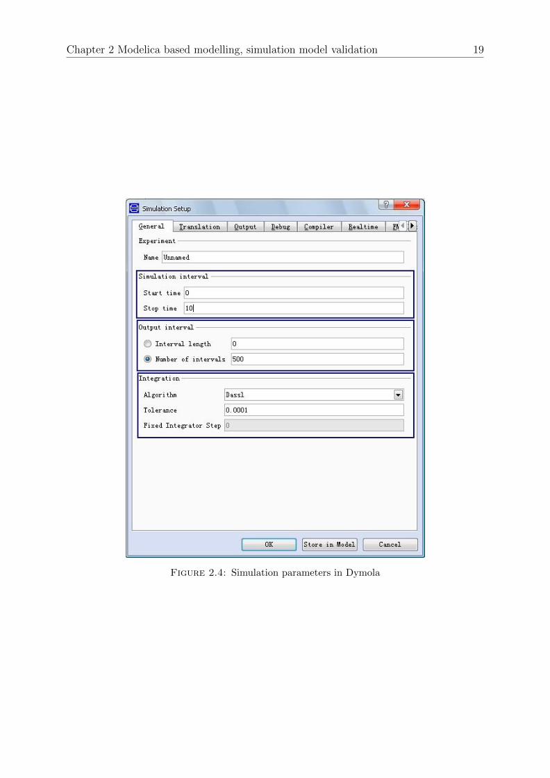
2.4 Simulation parameters
The setting of simulation parameters is important before starting the simulation. The
setting will affect the simulation result to a large extent. There are three groups of
simulation parameters:
1. Simulation interval. The time interval of simulation is set by start time and stop
time, as shown in Figure 2.4.
2. Output interval. The length of output intervals can be set in two ways: intervals
length and number of intervals, as shown in Figure 2.4. One can get smooth plots
by setting small interval length, but the simulation time will increase; on the other
hand if interval length is too large, the plot may be distorted to some extent, but
the simulation time will decrease.
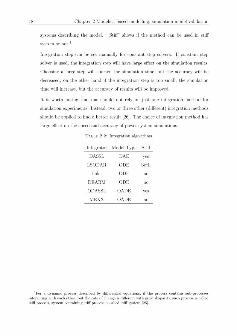
3. Integration algorithm. Dymola provides a number of different integration meth-
ods for the simulation of dynamic systems. The commonly used algorithms are
summarized in Table 2.2. In the table, “model type” means the type of equation
18 Chapter 2 Modelica based modelling, simulation model validation
systems describing the model. “Stiff” shows if the method can be used in stiff
system or not 1.
Integration step can be set manually for constant step solvers. If constant step
solver is used, the integration step will have large effect on the simulation results.
Choosing a large step will shorten the simulation time, but the accuracy will be
decreased; on the other hand if the integration step is too small, the simulation
time will increase, but the accuracy of results will be improved.
It is worth noting that one should not rely on just one integration method for
simulation experiments. Instead, two or three other (different) integration methods
should be applied to find a better result [26]. The choice of integration method has
large effect on the speed and accuracy of power system simulations.
Table 2.2: Integration algorithms
Integrator Model Type Stiff
DASSL DAE yes
LSODAR ODE both
Euler ODE no
DEABM ODE no
ODASSL OADE yes
MEXX OADE no
1For a dynamic process described by differential equations, if the process contains sub-processesinteracting with each other, but the rate of change is different with great disparity, such process is calledstiff process, system containing stiff process is called stiff system [26].
Chapter 2 Modelica based modelling, simulation model validation 19
Figure 2.4: Simulation parameters in Dymola


Chapter 3
Modelling of Power System
Components in Modelica
3.1 Introduction
This chapter presents the detailed modelling procedures and validation results of power
system components in Modelica. The objective of the modelling is to create correct and
reusable models that can function well with other power system models. Since some
basic models (e.g. buses, transmission lines, transformers etc.) are available from former
works [27], the emphasis of this thesis is on the modelling of control components in power
system.
In order to model the components correctly, the modelling are based on other software,
which are used as references. The referenced software in this thesis are PSAT, PSS/E
and Simulink. Since the ways reference software working are completely different from
Modelica, a new modelling approach needs to be taken. The steps to achieve a successful
modelling are as following:
1. Read the specification of the model, understand the conceptual background of the
model.
2. Identify the equations that describe the dynamic behaviour of the model.
21

22 Chapter 3 Modelling of Power System Components in Modelica
3. Write the model in Modelica.
4. Initialize the model.
5. Perform software-to-software validation of the Modelica model against the reference
model.
In order to present the basic processes, a few models are presented in this chapter. The
models include:
• Synchronous generator models (reference software: PSAT)
• Turbine governor TG1 (reference software: PSAT)
• Excitation system EXAC1 (reference software: PSS/E)
• Power system stabilizer (reference software: PSS/E)
• Load tap changers (reference software: Simulink)
The rest models and validation results can be found in appendix A.
3.2 Power system components modelling principles
As stated above, the objective of modelling is to create correct and reusable models for
power system components. To achieve this objective, the following principles need to be
followed:
• Define the model in the most direct and easiest way. Modelica allows
defining a model using other models, thus when constituent models are available, the
user can simply connect models together to form a new model, without transferring
the entire model into equations. Therefore the first step of modelling is to find the
most direct way to represent the model.

Chapter 3 Modelling of Power System Components in Modelica 23
• Define and state parameters, constants, and variables clearly. In Modelica,
constants do not change with time and cannot be modified; whereas parameters
are constant with time but can be modified; and variables are varied with time
and commonly used in equations. The type of model inputs and outputs must be
defined and stated distinctly.
• Place the parameters on the top layer of a model block. In order to reuse
the models conveniently, the model parameters must be displayed on the top layer
of the block to be modified easily. Especially for the models made up of other
components, parameters of the constituent components must be propagated onto
the top layer.
• Use connectors as input and output interfaces. The model inputs and outputs
must be verified before the modelling, and corresponding types of connectors are
used as interface to other models.
• Select the proper initialization method. One can initialize models either
through auxiliary parameters, or through initial equations.
• Design the model appearance concisely. The model should be one simple
block. If the model is formed by connecting other models, one must aggregate them
in one block or icon.
• Organize the models in packages. Package is an easy method to organize
models in a structured way. Models can be grouped of similar type in one package,
which makes it easier to find a particular model in the applications.
3.3 Implementation of models in Modelica
3.3.1 Synchronous generators
This section describes the modelling of synchronous generators. Two different generator
models are implemented according to the mathematical models in PSAT [2]. In PSAT

24 Chapter 3 Modelling of Power System Components in Modelica
generator models, various simplifications can be applied, and the models are divergent
from the basic model with only classical swing equation to an eight order model with
field saturation. In the two models presented in this section, the dynamic of transient
and sub-transient voltage are additionally considered. The models differ mainly in the
differential equations.
The algebraic equation system for synchronous generator models is specified in Appendix
A.1.1, as shown in equation A.2 - A.7.
3.3.1.1 Forth Order
The variables and parameters of the forth order generator model are detailed in Table
A.1 and A.2. Other than parameters and variables, auxiliary parameters are defined to
initialize the variables. The models are initialized after power flow computations. Once
the power flow solution are determined, v0, θ0, p0, q0, and v0f at the generator bus are
used for initializing the variables. The initial values of variables are specified in Table
A.3.
In this model, besides the classical electro-mechanical model, lead-lag functions are used
for modelling the d and q-aixs inductances. Electromagnetic flux dynamics is neglected,
thus leading to a fourth order system in the state variables δ, ω, e′q and e′d. The differential
equations are:
δ = Ωb(ω − 1)
ω = (Pm − P −D(ω − 1))/M
e′q = (−e′q − (xd − x′d)id + v∗f )/T′d0
e′d = (−e′d + (xq − x′q)iq)/T ′q0
(3.1)
Where
Ωb = 2πfn
v∗f = vf +Kω(ω − 1)−Kp(P − P0)(3.2)
Chapter 3 Modelling of Power System Components in Modelica 25
The voltage and current link is described by the equation:
e′q = vq + raiq + x′did
e′d = vd + raid − x′qiq(3.3)
Equation A.2 - A.7 and 3.1 - 3.3 form the equations of forth order generator model.
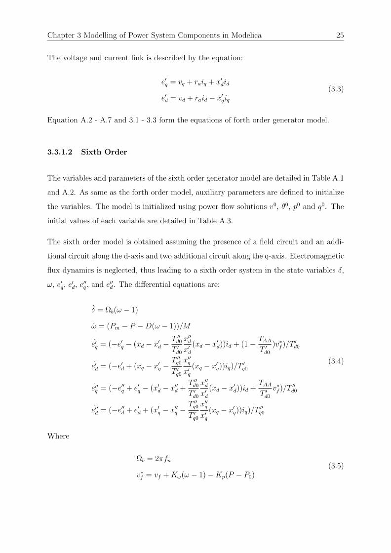
3.3.1.2 Sixth Order
The variables and parameters of the sixth order generator model are detailed in Table A.1
and A.2. As same as the forth order model, auxiliary parameters are defined to initialize
the variables. The model is initialized using power flow solutions v0, θ0, p0 and q0. The
initial values of each variable are detailed in Table A.3.
The sixth order model is obtained assuming the presence of a field circuit and an addi-
tional circuit along the d-axis and two additional circuit along the q-axis. Electromagnetic
flux dynamics is neglected, thus leading to a sixth order system in the state variables δ,
ω, e′q, e′d, e
′′q , and e′′d. The differential equations are:
δ = Ωb(ω − 1)
ω = (Pm − P −D(ω − 1))/M
e′q = (−e′q − (xd − x′d −T ′′d0T ′d0
x′′dx′d
(xd − x′d))id + (1− TAAT ′d0
)v∗f )/T′d0
e′d = (−e′d + (xq − x′q −T ′′q0T ′q0
x′′qx′q
(xq − x′q))iq)/T ′q0
e′′q = (−e′′q + e′q − (x′d − x′′d +T ′′d0T ′d0
x′′dx′d
(xd − x′d))id +TAAT ′d0
v∗f )/T′′d0
e′′d = (−e′′d + e′d + (x′q − x′′q −T ′′q0T ′q0
x′′qx′q
(xq − x′q))iq)/T ′′q0
(3.4)
Where
Ωb = 2πfn
v∗f = vf +Kω(ω − 1)−Kp(P − P0)(3.5)

26 Chapter 3 Modelling of Power System Components in Modelica
e′′q = vq + raiq + x′′did
e′′d = vd + raid − x′′q iq(3.6)
3.3.2 Turbine Governor
Turbine governors define the primary frequency control of synchronous machines. The
turbine governor model (TG1) implemented in Modelica is shown in Figure 3.1. The
reference model is originally developed in PSAT. As shown in the block diagram, the
model has three input signals: the actual rotor speed ω, the reference rotor speed ωref ,
and the reference active power pref . Output of the model is the mechanical power Pm to
be applied to generator.
The governor regulates the speed of the generator by comparing its output with a prede-
fined reference. When R 6= 0 and R <∞, the governor regulates the speed proportionally
to its power rate. In the mechanical part, two lead-lag filters are used to stand for the
servo motor and the reheat mechanism.
Figure 3.1: Block diagram of turbine governor model TG1 [2]
The variables and parameters of the turbine governor model are detailed in Table A.4
and A.5. Auxiliary parameters are also defined to initialize the variables of the model.
The initial values of each variable are the values at the equilibrium point (e.g. ω0 and
p0). The initialization parameter are detailed in Table A.6.
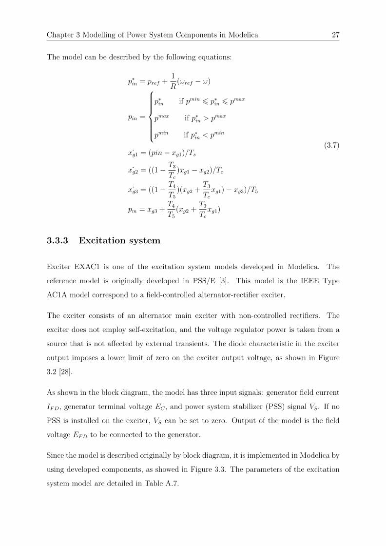
Chapter 3 Modelling of Power System Components in Modelica 27
The model can be described by the following equations:
p∗in = pref +1
R(ωref − ω)
pin =
p∗in if pmin 6 p∗in 6 pmax
pmax if p∗in > pmax
pmin if p∗in < pmin
˙xg1 = (pin− xg1)/Ts
˙xg2 = ((1− T3Tc
)xg1 − xg2)/Tc
˙xg3 = ((1− T4T5
)(xg2 +T3Tcxg1)− xg3)/T5
pm = xg3 +T4T5
(xg2 +T3Tcxg1)
(3.7)
3.3.3 Excitation system
Exciter EXAC1 is one of the excitation system models developed in Modelica. The
reference model is originally developed in PSS/E [3]. This model is the IEEE Type
AC1A model correspond to a field-controlled alternator-rectifier exciter.
The exciter consists of an alternator main exciter with non-controlled rectifiers. The
exciter does not employ self-excitation, and the voltage regulator power is taken from a
source that is not affected by external transients. The diode characteristic in the exciter
output imposes a lower limit of zero on the exciter output voltage, as shown in Figure
3.2 [28].
As shown in the block diagram, the model has three input signals: generator field current
IFD, generator terminal voltage EC , and power system stabilizer (PSS) signal VS. If no
PSS is installed on the exciter, VS can be set to zero. Output of the model is the field
voltage EFD to be connected to the generator.
Since the model is described originally by block diagram, it is implemented in Modelica by
using developed components, as showed in Figure 3.3. The parameters of the excitation
system model are detailed in Table A.7.

28 Chapter 3 Modelling of Power System Components in Modelica
Figure 3.2: Block diagram of excitation system model EXAC1 [3]
Figure 3.3: Excitation system model EXAC1 in Modelica
Chapter 3 Modelling of Power System Components in Modelica 29
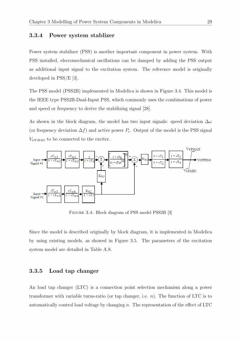
3.3.4 Power system stablizer
Power system stabilizer (PSS) is another important component in power system. With
PSS installed, elecromechanical oscillations can be damped by adding the PSS output
as additional input signal to the excitation system. The reference model is originally
developed in PSS/E [3].
The PSS model (PSS2B) implemented in Modelica is shown in Figure 3.4. This model is
the IEEE type PSS2B-Dual-Input PSS, which commonly uses the combinations of power
and speed or frequency to derive the stabilizing signal [28].
As shown in the block diagram, the model has two input signals: speed deviation ∆ω
(or frequency deviation ∆f) and active power Pe. Output of the model is the PSS signal
VOTHSG to be connected to the exciter.
Figure 3.4: Block diagram of PSS model PSS2B [3]
Since the model is described originally by block diagram, it is implemented in Modelica
by using existing models, as showed in Figure 3.5. The parameters of the excitation
system model are detailed in Table A.8.
3.3.5 Load tap changer
An load tap changer (LTC) is a connection point selection mechanism along a power
transformer with variable turns-ratio (or tap changer, i.e. n). The function of LTC is to
automatically control load voltage by changing n. The representation of the effect of LTC

30 Chapter 3 Modelling of Power System Components in Modelica
Figure 3.5: PSS model PSS2B in Modelica
transformer is particularly important for the analysis of slow voltage collapse phenomena
[29].
The dynamic of LTC is described by a discrete tap changing logic. To keep the load
voltage in the deadband [Vmin, Vmax] p.u., the LTC adjusts the transformer ratios in the
range [nmin, nmax] over N positions (thus from one position to the next, the ratio varies
by (nmax − nmin)/(N − 1)).
The LTC has intentional delays. When the load voltage leaves the deadband at time
t0, the first tap change takes place at time t0 + τ1 and the subsequent changes at times
t0 + τ1 + kτ2 (k = 1, 2, ...). The delay is reset to τ1 after the controlled voltage has re-
entered (or jumped from one side to the other of) the deadband. The values of τ1 and τ2
differ from one transformer to another in order to avoid unrealistic tap synchronization
[5].
The LTC model implemented in Modelica is shown in Figure 3.6. As shown in the block
diagram, input and output of the model are the load voltage vl and turns-ratio n. The
parameters of the LTC model are detailed in Table A.9.
3.4 Model validation
To assure the accuracy of modelling, software-to-software validation is carried out by
designing different test scenarios. This procedure requires to compare outputs of two

Chapter 3 Modelling of Power System Components in Modelica 31
Figure 3.6: Block diagram of LTC model
validation systems given the same input and the same system structure (parameters). A
correct model will provide a one to one match between the corresponding output signals.
3.4.1 Software-to-software validation
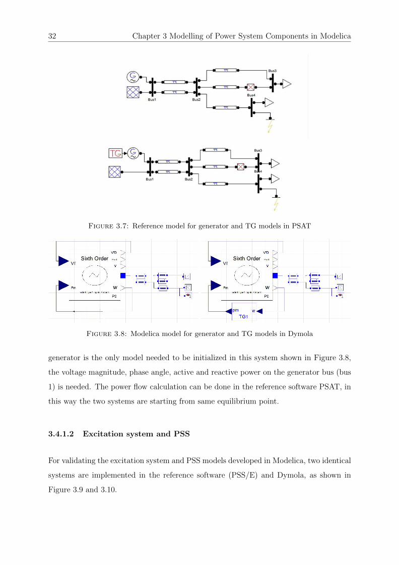
3.4.1.1 Generator and turbine governor
For validating the generator and TG models developed in Modelica, two identical systems
are implemented in the reference software (PSAT) and Dymola, as shown in Figure 3.7
and 3.8. The model of generator and TG model are connected to a 4-bus-system with
two constant PQ loads. To investigate the dynamic response of the models, two kinds of
disturbance are applied to the system:
1. A three-phase short-circuit fault lasting 100ms is located on bus 4.
2. One of the parallel transmission lines between bus 2 and bus 4 is tripped for 100ms
from t = 3s to t = 3.1s.
This structure was chosen in order to avoid locating the fault directly on the generator
terminal, thus the fault is less severe.
In order to commence the dynamic simulation, the model needs to be initialized. Power
flow solution can be used to present the equilibrium point before the disturbance. Since
32 Chapter 3 Modelling of Power System Components in Modelica
Figure 3.7: Reference model for generator and TG models in PSAT
Figure 3.8: Modelica model for generator and TG models in Dymola
generator is the only model needed to be initialized in this system shown in Figure 3.8,
the voltage magnitude, phase angle, active and reactive power on the generator bus (bus
1) is needed. The power flow calculation can be done in the reference software PSAT, in
this way the two systems are starting from same equilibrium point.
3.4.1.2 Excitation system and PSS
For validating the excitation system and PSS models developed in Modelica, two identical
systems are implemented in the reference software (PSS/E) and Dymola, as shown in
Figure 3.9 and 3.10.

Chapter 3 Modelling of Power System Components in Modelica 33
Figure 3.9: Reference model for excitation system and PSS models in PSS/E
Figure 3.10: Modelica model for excitation system and PSS models in Dymola
Similar to the validation system for generator and TG models, the system is a 4-bus-
system with one sixth order generator and two constant PQ loads. However in order to
simplify the simulation process in PSS/E, one of the disturbances is omitted. In another
words, only the short-circuit fault on bus 4 is applied to the system. The fault is also
lasting for 100ms.
Power flow solution is used in the initialization process of the system similarly. The data
of voltage magnitude, phase angle, active and reactive power on the generator bus (bus
1) is used. The power flow calculation are performed in the reference software PSS/E, so
that the two systems are starting from the same equilibrium point.
34 Chapter 3 Modelling of Power System Components in Modelica
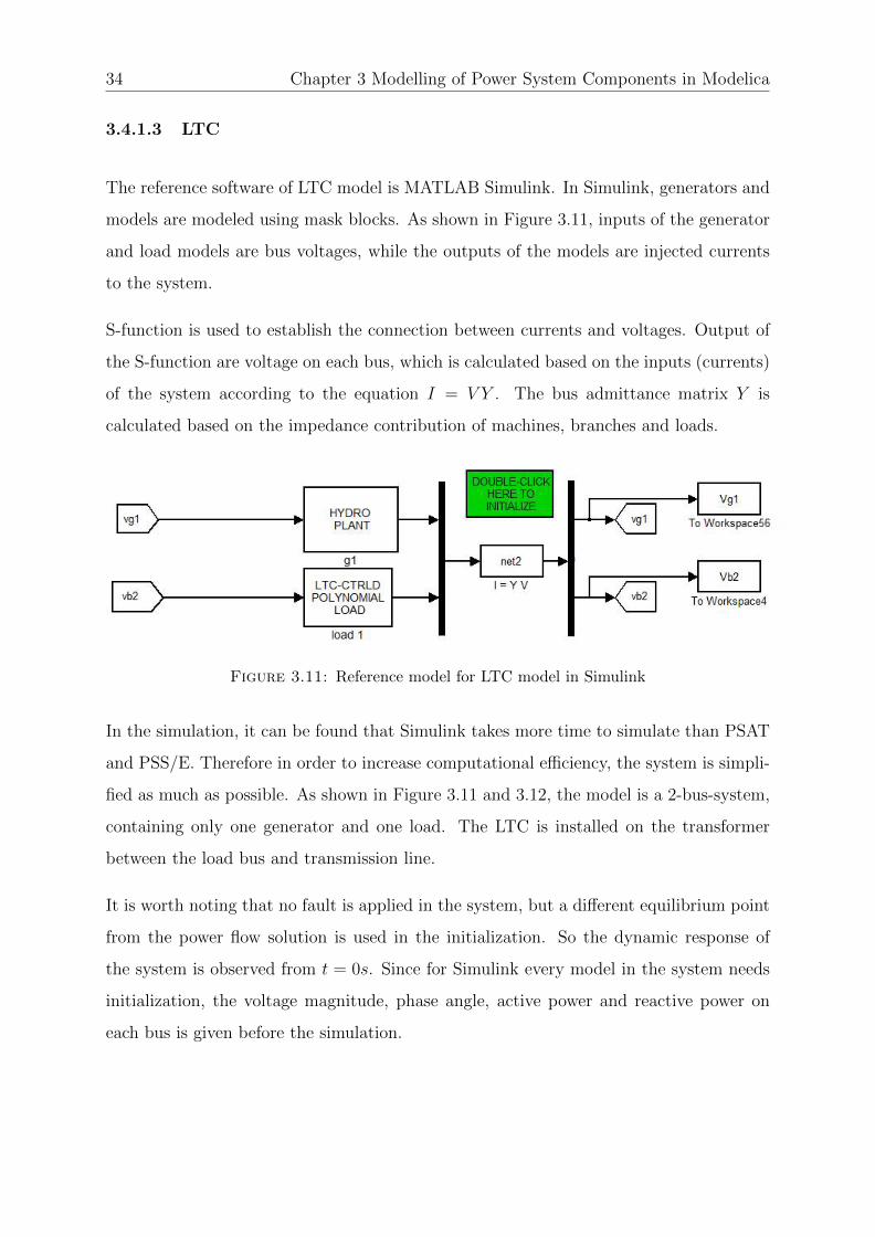
3.4.1.3 LTC
The reference software of LTC model is MATLAB Simulink. In Simulink, generators and
models are modeled using mask blocks. As shown in Figure 3.11, inputs of the generator
and load models are bus voltages, while the outputs of the models are injected currents
to the system.
S-function is used to establish the connection between currents and voltages. Output of
the S-function are voltage on each bus, which is calculated based on the inputs (currents)
of the system according to the equation I = V Y . The bus admittance matrix Y is
calculated based on the impedance contribution of machines, branches and loads.
Figure 3.11: Reference model for LTC model in Simulink
In the simulation, it can be found that Simulink takes more time to simulate than PSAT
and PSS/E. Therefore in order to increase computational efficiency, the system is simpli-
fied as much as possible. As shown in Figure 3.11 and 3.12, the model is a 2-bus-system,
containing only one generator and one load. The LTC is installed on the transformer
between the load bus and transmission line.
It is worth noting that no fault is applied in the system, but a different equilibrium point
from the power flow solution is used in the initialization. So the dynamic response of
the system is observed from t = 0s. Since for Simulink every model in the system needs
initialization, the voltage magnitude, phase angle, active power and reactive power on
each bus is given before the simulation.

Chapter 3 Modelling of Power System Components in Modelica 35
Figure 3.12: Modelica model for LTC model in Dymola
3.4.2 Validation results
In this section the validation results of the models described above are presented. In
the results outputs from the reference software and Dymola are compared. When the
corresponding output signals match each other, one can say the model is validated.
Validation results of all models can be found in Appendix A.
3.4.2.1 Forth Order generator
For the forth order generator model, the output signals compared are active power P , re-
active power Q, d-axis transient voltage e′d, q-axis transient voltage e′q, generator terminal
voltage vg and rotor speed ω. The plots are shown in Figure A.1.
Discussion: After the disturbances applied at t = 3s and t = 12s, the two systems
response in the identical way. Since the model provide an one-to-one match between
the corresponding output signals, the forth order generator model can be concluded as
validated.

36 Chapter 3 Modelling of Power System Components in Modelica
3.4.2.2 Sixth Order generator
For the sixth order generator model, the output signals compared are active power P ,
reactive power Q, d-axis transient voltage e′d, q-axis transient voltage e′q, d-axis sub-
transient voltage e′′d, q-axis sub-transient voltage e′′q , generator terminal voltage vg and
rotor speed ω. The plots are shown in Figure A.2.
Discussion: After the disturbances applied at t = 3s and t = 12s, the output signals
match each other perfectly, including the sub-transient response. Thus the sixth order
generator model can be concluded as validated.
3.4.2.3 Turbine governor
For the turbine governor model TG1, the compared output signals are Pm and ω. Pm
is the mechanical power applied to generator, which is the only output of the governor
model; while ω is the generator rotor speed, which is the state variable directly controlled
by the governor. The plots are shown in Figure A.3.
Discussion: The outputs from two systems are identical. After the disturbances applied
at t = 3s and t = 12s, the turbine governor controls the mechanical power to stabilize
the rotor speed. After 15 seconds, the rotor speed is stabilized at ω = 1 p.u., and
the mechanical power is stabilized at Pm = 0.16 p.u., equal to the values before the
disturbances.
It is worth noting that the CPU-time for integration is 0.525 seconds in Dymola, while
is 15.9799 seconds in PSAT. It can be seen that Modelica allowed a reduction of the
integration step without increasing the computation time, thus providing smoother and
more accurate results.
3.4.2.4 Excitation system
For the excitation system model EXAC1, the compared output signals are vf and vg.
vf is the field voltage applied to generator, which is the only output of the excitation
Chapter 3 Modelling of Power System Components in Modelica 37
system. vg is generator terminal voltage, which is the state variable directly controlled
by the excitation system. The plots are shown in Figure A.4.
Discussion: The two systems response in the identical way. After the short-circuit
fault applied at t = 2s, the terminal voltage vg decreases instantaneously. To recover
the system voltage, the excitation system increases field voltage vf , then the generator
terminal voltage is controlled and stabilized at vg = 1 p.u. after 3 seconds.
It can be observed that there exist small differences between the initial conditions in
Figure A.4. The reason of the different initial condition is that the initialization processes
of generator models in Modelica model and PSS/E model are not exactly the same.
However it can be seen that after 0.5’s fluctuation, the steady-state condition before
disturbance of two system models are the same. The deviation does not influence the
validation of excitation system model.
3.4.2.5 PSS
For the power system stabilizer model PSS2B, the outputs of PSS model Upss are com-
pared. The plots are shown in Figure A.5.
Discussion: As seen in Figure A.5, the two output signals match well. After the short-
circuit applied at t = 2s, the PSS is activated to provide stabilizing signal; after t = 8s,
the oscillation in the system is damped, resulting in Upss turning back to 0.
3.4.2.6 LTC
For the load tap changer model LTC, the compared output signals are vload and rb. vload
is the load bus voltage, while rb is the transformer ratio controlled by LTC. The plots are
shown in Figure A.6.
Discussion: As shown in Figure A.6, the output signals from two systems match well.
Since the initial value of Vload is above the deadband, the LTC adjusts the transformer
ratios from rb = 1. The first tap change takes place at t = t0 + t1 + τ1 = 0 + 10 = 10s,
and the subsequent changes at times t0 + τ1 + kτ2 (k = 1, 2, · · · ) = 15s, 20s, 25s, · · · .

38 Chapter 3 Modelling of Power System Components in Modelica
After the actions of LTC, the load bus voltage is adjusted at vload = 0.996 p.u., which is
within the deadband.
The CPU-time for integration is 0.435 seconds in Dymola, while is 28 seconds in Simulink.
It is proved that Modelica computation power allows a reduction of the integration step
without increasing the computation time.

Chapter 4
Modelling and Dynamic Simulation
of Power Systems in Modelica
4.1 Introduction
With necessary component models prepared, it is theoritically feasible to implemente and
simulate integral power system models in Modelica. This chapter presents the experiences
of power system modelling and dynamic simulation in Modelica.
In this thesis, four systems of different scale are implemented. The systems models will
be used in future work in studying different aspect of problem, such as voltage stability
analysis, instability detection and control.
• KTH Nordic 32 system: a conceptualization of the Swedish power system and its
neighbors circa 1995, with some adjustment of the system model [4].
• IEEE Nordic 32 system: the IEEE Nordic 32 voltage stability test model
• iGrGen system: a model of a generator plant in Greece
• INGSVC system: a model of a sub-set of National Grid’s network including two
SVCs
39

40 Chapter 4 Modelling and Dynamic Simulation of Power Systems in Modelica
The test systems are originally developed in different softwares. For instance, KTH Nordic
32 system model was developed in PSAT, whereas INGSVC system model was described
specifically in PowerFactory. In the modelling process, the original models implemented
in other software are regarded as references.
Software-to-software validation of the system models is done through the comparison of
simulation results from different software. Given the same system structure, component
model and critical system data, the system in Modelica should response in a same manner
as the reference system. Nevertheless, it is worth noting that for large scale systems, it
is more difficult than small scale systems to obtain exactly same responses. In this case
the criterion of validation should be revised on a case-by-case basis.
4.2 Power system modelling principles
As stated above, the objective of modelling is to create integral and correct test system
models which can be used as benchmark systems in different studies. To achieve the
objectives, the following five principles need to be followed:
1. The study purposes of the test system need to be determined
Test systems for one particular study should include specific representation of power
system elements that have significant impact on the study. Therefore the usage of test
systems must be determined clearly at the start of modelling to avoid omitting important
elements. For instance, the IEEE Nordic 32 system is designed for voltage stability
analysis and security assessment. Therefore the system model should include elements
with the following characteristics [30–32]:
• Generator characteristics with excitation system models and its operating limits.
Over excitation limiter (OEL) should be explicitly represented in order to account
for the enforcement of generator limits.
• Transmission system reactive compensating devices characteristics or network com-
pensation devices such as shunt capacitors, regulated shunt compensation, and series
capacitors. Effect of transmission level LTC transformers should be accounted.

Chapter 4 Modelling and Dynamic Simulation of Power Systems in Modelica 41
• Load characteristics with voltage dependence of loads and load restoration mech-
anisms (through the actions of load tap changers on transformers feeding the dis-
tribution system, and other load restoration mechanism such as those involving
thermostat and some other load regulation devices). It is also important to account
the effects of reactive power sources in the distribution systems.
• Other protection and controls which include armature overcurrent protection, trans-
mission line overcurrent protection, reactive power source controls, and undervolt-
age load shedding.
Depend on different power system characteristics and prevailing operation conditions, it
may be also necessary to include frequency dependence of loads, explicit model of auto-
matic generation control (AGC), phase-shifting regulators, account the effect of adjustable
ratio of generator step-up transformers and secondary voltage control.
2. Make appropriate simplification to the system model
Modern interconnected electric power systems cover very large geographic areas, include
a large amount of electrical or non-electrical devices. To do one particular kind of study
in the systems, it is neither practical nor necessary to model in detail the entire inter-
connected system [33]. It is common practice to represent parts of the system by some
form of simplified model. The desired characteristics of the simplified model depends on
its application and usage.
For most applications, two simplification approaches are commonly used. The first one is
network simplification using equivalent techniques. In this approach, the interconnected
power systems are partitioned into a studied area that needs to be well represented, and
external areas that can be replaced by equivalent models [34]. Through this approach,
the scale of the system can be reduced significantly.
The second commonly used approach is simplification of generator models. Generator
is one of the most complex models in power system modelling. Thus by simplifying the
model into several reduced orders, the amount of state variables in the system model will
be decreased.
42 Chapter 4 Modelling and Dynamic Simulation of Power Systems in Modelica
3. Use power flow solution to initialize the system model
The simulation of power system commonly starts from a equilibrium point, in which
the system status can be presented by power flow solutions. The power flow calculation
can be done in the reference software. To initialize the system model conveniently, the
initialization parameters should be placed on top level of the system model.
4. The configuration of system model should be concise and compact
In the modelling of large scale power systems, it is important to organize the model in
a concise and compact manner. It is common to include dozens of buses and hundreds
of components in one system model, only one fault in the connection will lead to failed
simulation. Thus for the convenience of double checking the configuration of the model
should be as concise and compact as possible.
5. Implement the system model in a hierarchical approach
Modelica provides the possibility to implement power system models in a hierarchical
way. Because of Modelica models can be implemented by connecting other models, some
parts of power system (such as power plant models with generators and other control
elements, and transformers with LTC) can be integrated into one compact model and
used in the modelling of system. Figure 4.1 shows an example of hydro power plant
model in Modelica. The models of generator, hydro turbine and speed governor are
integrated into the hydro plant model, which can be used directly in the modelling of
power system.
The system models are originally developed in PSAT, Simulink and Powerfactory. Since
the modelling method in reference software are different from Modelica, a new set of
procedures needs to be followed . The steps to achieve a successful modelling are as
following:
1. Read the specification of the system. If detailed component models are not provided,
select components to be included in the system model according to the application
and use.
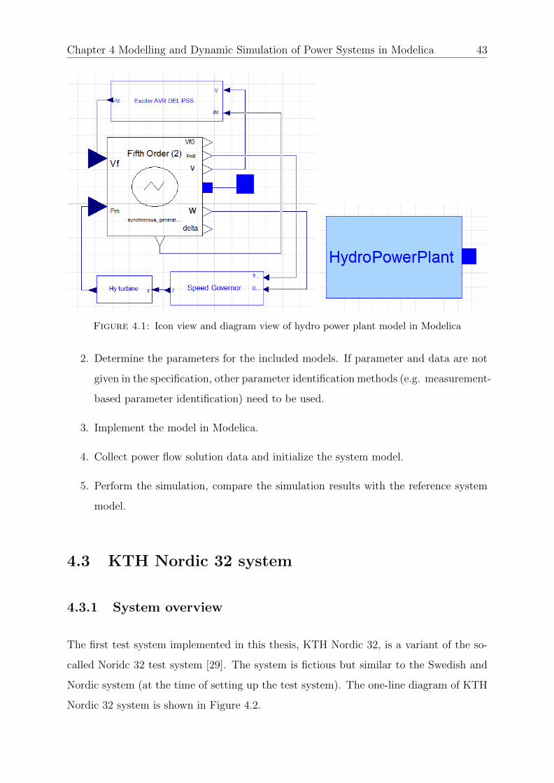
Chapter 4 Modelling and Dynamic Simulation of Power Systems in Modelica 43
Figure 4.1: Icon view and diagram view of hydro power plant model in Modelica
2. Determine the parameters for the included models. If parameter and data are not
given in the specification, other parameter identification methods (e.g. measurement-
based parameter identification) need to be used.
3. Implement the model in Modelica.
4. Collect power flow solution data and initialize the system model.
5. Perform the simulation, compare the simulation results with the reference system
model.
4.3 KTH Nordic 32 system
4.3.1 System overview
The first test system implemented in this thesis, KTH Nordic 32, is a variant of the so-
called Noridc 32 test system [29]. The system is fictious but similar to the Swedish and
Nordic system (at the time of setting up the test system). The one-line diagram of KTH
Nordic 32 system is shown in Figure 4.2.

44 Chapter 4 Modelling and Dynamic Simulation of Power Systems in Modelica
The system involves 20 generators, 32 transmission and 22 distribution buses, for a total
of 74 buses. The test system is divided into four areas:
• “North” with hydro generation and some load
• “Central” with much load and thermal power generation
• “Equiv” connected to the “North”, it includes a simple equivalent of an external
system
• “South” with thermal generation, rather loosely connected to the rest of the system
Among the 20 generators in the system, 12 of which are hydro generators located in
the North and Equivalent areas, whereas the rest are thermal generators located in the
Central and South area. The system is heavily loaded with large transfers essentially
from North to Central areas, which easily leads to system instabilities.
The nominal frequency is 50 Hz. Frequency is controlled by the speed governors in the
hydro power plant in the North and Equiv areas. G20 is an equivalent generator, with a
large participation in primary frequency control. The thermal units of the Central and
South areas do not participate in this control.
The maximum power that can be delivered to the Central loads is strongly influenced
by the reactive power capabilities of the Central and some of the Northern generators.
Their reactive power limits are enforced by over excitation limiters (OELs). If, after a
disturbance (such as a line outage), the power that need to be delivered is larger than
the generator limits, voltage instability will be resulted.
The KTH Nordic 32 system is originally implemented in PSAT, which is considered as
reference for the system model in Modelica.
4.3.2 Model and data
1. Buses: The system has 52 node buses, 20 of which are generator buses. There are
four level of voltages; 15 kV for generator buses, 20kV for distribution buses, 130
kV, 220 kV and 400 kV for transmission buses.
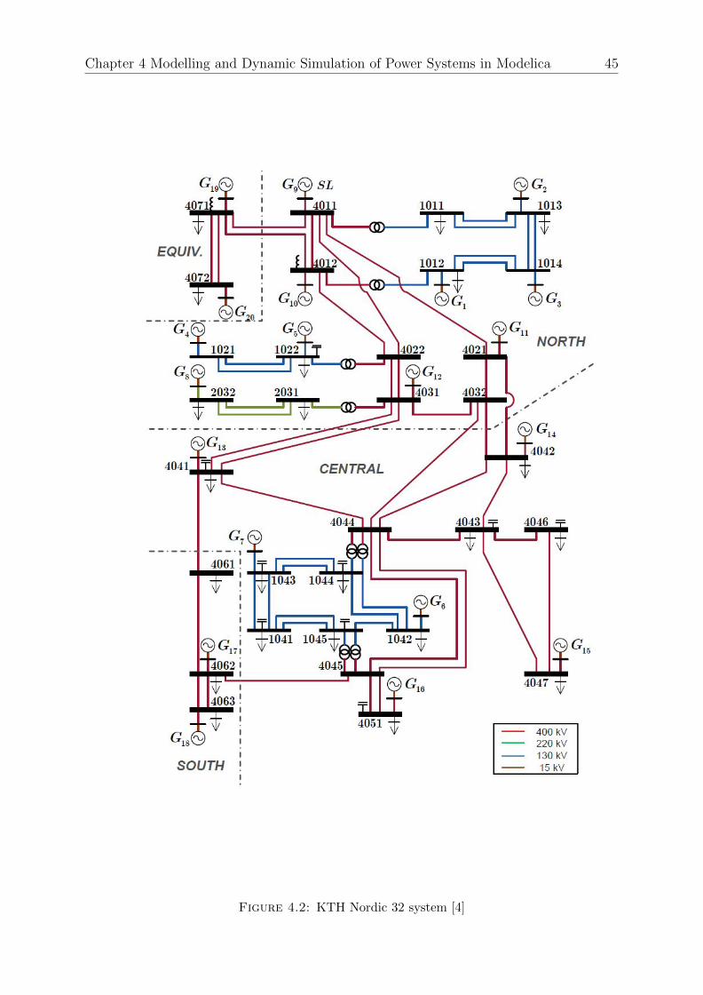
Chapter 4 Modelling and Dynamic Simulation of Power Systems in Modelica 45
Figure 4.2: KTH Nordic 32 system [4]

46 Chapter 4 Modelling and Dynamic Simulation of Power Systems in Modelica
2. Transmission lines: The system has 52 transmission lines in total. The trans-
mission line model is based on the π-equivalent circuit. The values for resistance r,
reactance x and susceptance b are in per unit. Shunt conductance is not considered
in this model.
3. Loads: The loads in the system are modeled as constant impedance loads. In
the initialization of the model, with node voltage magnitude U0, load active power
P0 and reactive power Q0 from power flow solution are transformed into constant
impedances Rl and Xl:
P0 =RlU
20
R2l +X2
l
, Q0 =XlU
20
R2l +X2
l
(4.1)
4. Shunts: The system has 11 shunts, 9 of which are capacitor banks and the rest are
inductor banks. The capacitive shunts are represented by positive susceptance b,
whereas the inductive shunts are represented by negative b. The description of the
shunt model can be seen in appendix A.4.
5. Synchronous generators: Two synchronous generator models are used in the
system: three rotor windings for the salient-pole machines of hydro power plants
(Order V Type 2) and four windings for the round-rotor machines of thermal power
plants (Order VI). All data follows Van Cutsem’s proposed data [35], except for the
nominal apparent power of G18 that is changed to 1600 MVA. Saturation effects are
neglected.
6. Turbine governors: Two types of turbine governors are employed in the system.
TG Type I is used for the thermal generators while TG Type II is used for the hydro
generators. The data for hydro TGs is provided in [35], whereas recommended
values are applied for the thermal TGs. The TG Type II model is depicted in
Figure 4.3, and the TG Type I model is described in Chapter 3.3.2.
7. Automatic voltage regulators: Automatic voltage regulators (AVR) are used
for all generators to control the field voltage vf . The AVR model used in the system
is AVR Type III [2]. The AVR model is depicted in Figure 4.4, and the parameters
are the recommended values provided in [36].
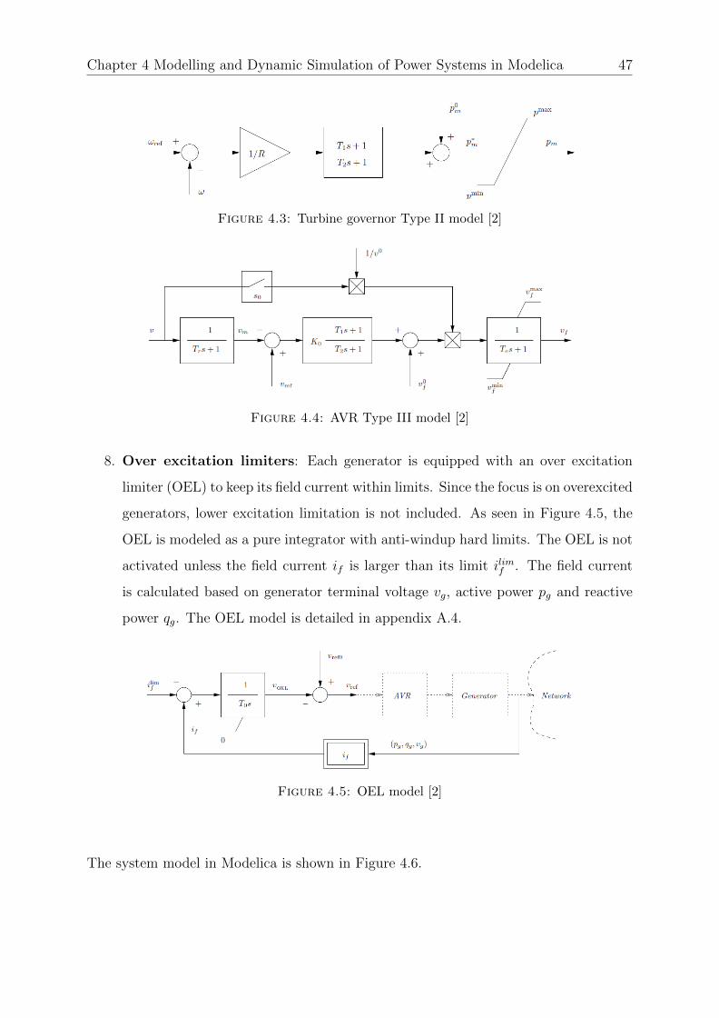
Chapter 4 Modelling and Dynamic Simulation of Power Systems in Modelica 47
Figure 4.3: Turbine governor Type II model [2]
Figure 4.4: AVR Type III model [2]
8. Over excitation limiters: Each generator is equipped with an over excitation
limiter (OEL) to keep its field current within limits. Since the focus is on overexcited
generators, lower excitation limitation is not included. As seen in Figure 4.5, the
OEL is modeled as a pure integrator with anti-windup hard limits. The OEL is not
activated unless the field current if is larger than its limit ilimf . The field current
is calculated based on generator terminal voltage vg, active power pg and reactive
power qg. The OEL model is detailed in appendix A.4.
Figure 4.5: OEL model [2]
The system model in Modelica is shown in Figure 4.6.

48 Chapter 4 Modelling and Dynamic Simulation of Power Systems in Modelica
Figure 4.6: KTH Nordic 32 system model in Modelica
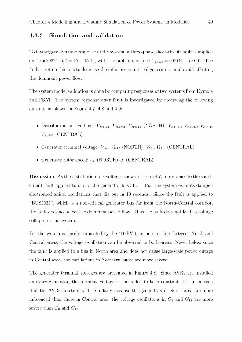
Chapter 4 Modelling and Dynamic Simulation of Power Systems in Modelica 49
4.3.3 Simulation and validation
To investigate dynamic response of the system, a three-phase short-circuit fault is applied
on “Bus2032” at t = 15− 15.1s, with the fault impedance Zfault = 0.0001 + j0.001. The
fault is set on this bus to decrease the influence on critical generators, and avoid affecting
the dominant power flow.
The system model validation is done by comparing responses of two systems from Dymola
and PSAT. The system response after fault is investigated by observing the following
outputs, as shown in Figure 4.7, 4.8 and 4.9:
• Distribution bus voltage: VB4022, VB2032, VB4012 (NORTH) VB1041, VB1043, VB1045
VB4041 (CENTRAL)
• Generator terminal voltage: VG8, VG12 (NORTH) VG6, VG13 (CENTRAL)
• Generator rotor speed: ω8 (NORTH) ω6 (CENTRAL)
Discussion: As the distribution bus voltages show in Figure 4.7, in response to the short-
circuit fault applied to one of the generator bus at t = 15s, the system exhibits damped
electromechanical oscillations that die out in 10 seconds. Since the fault is applied to
“BUS2032”, which is a non-critical generator bus far from the North-Central corridor,
the fault does not affect the dominant power flow. Thus the fault does not lead to voltage
collapse in the system.
For the system is closely connected by the 400 kV transmission lines between North and
Central areas, the voltage oscillation can be observed in both areas. Nevertheless since
the fault is applied to a bus in North area and does not cause large-scale power outage
in Central area, the oscillations in Northern buses are more severe.
The generator terminal voltages are presented in Figure 4.8. Since AVRs are installed
on every generator, the terminal voltage is controlled to keep constant. It can be seen
that the AVRs function well. Similarly because the generators in North area are more
influenced than those in Central area, the voltage oscillations in G8 and G12 are more
severe than G6 and G13.
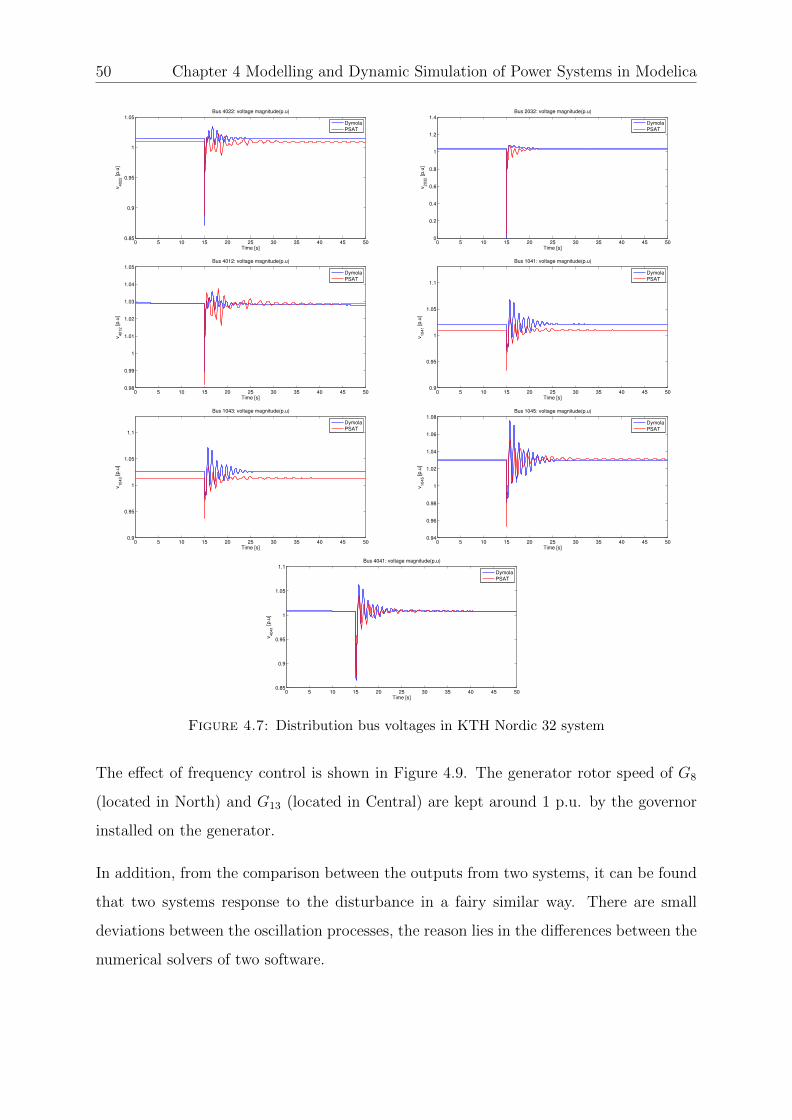
50 Chapter 4 Modelling and Dynamic Simulation of Power Systems in Modelica
0 5 10 15 20 25 30 35 40 45 500.85
0.9
0.95
1
1.05
Time [s]
v4022 [
p.u
]Bus 4022: voltage magnitude(p.u)
Dymola
PSAT
0 5 10 15 20 25 30 35 40 45 500
0.2
0.4
0.6
0.8
1
1.2
1.4
Time [s]
v2032 [
p.u
]
Bus 2032: voltage magnitude(p.u)
Dymola
PSAT
0 5 10 15 20 25 30 35 40 45 500.98
0.99
1
1.01
1.02
1.03
1.04
1.05
Time [s]
v4012 [
p.u
]
Bus 4012: voltage magnitude(p.u)
Dymola
PSAT
0 5 10 15 20 25 30 35 40 45 500.9
0.95
1
1.05
1.1
Time [s]
v1041 [
p.u
]
Bus 1041: voltage magnitude(p.u)
Dymola
PSAT
0 5 10 15 20 25 30 35 40 45 500.9
0.95
1
1.05
1.1
Time [s]
v1043 [p.u
]
Bus 1043: voltage magnitude(p.u)
Dymola
PSAT
0 5 10 15 20 25 30 35 40 45 500.94
0.96
0.98
1
1.02
1.04
1.06
1.08
Time [s]
v1045 [
p.u
]
Bus 1045: voltage magnitude(p.u)
Dymola
PSAT
0 5 10 15 20 25 30 35 40 45 500.85
0.9
0.95
1
1.05
1.1
Time [s]
v4041 [p.u
]
Bus 4041: voltage magnitude(p.u)
Dymola
PSAT
Figure 4.7: Distribution bus voltages in KTH Nordic 32 system
The effect of frequency control is shown in Figure 4.9. The generator rotor speed of G8
(located in North) and G13 (located in Central) are kept around 1 p.u. by the governor
installed on the generator.
In addition, from the comparison between the outputs from two systems, it can be found
that two systems response to the disturbance in a fairy similar way. There are small
deviations between the oscillation processes, the reason lies in the differences between the
numerical solvers of two software.
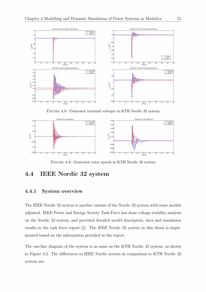
Chapter 4 Modelling and Dynamic Simulation of Power Systems in Modelica 51
0 5 10 15 20 25 30 35 40 45 500
0.2
0.4
0.6
0.8
1
1.2
1.4
Time [s]
vg8 [p.u
]
Generator 8: terminal voltage magnitude(p.u)
Dymola
PSAT
0 5 10 15 20 25 30 35 40 45 500.7
0.75
0.8
0.85
0.9
0.95
1
1.05
1.1
Time [s]
vg12 [p.u
]
Generator 12: terminal voltage magnitude(p.u)
Dymola
PSAT
0 5 10 15 20 25 30 35 40 45 500.97
0.98
0.99
1
1.01
1.02
1.03
1.04
1.05
1.06
1.07
Time [s]
vg6 [p.u
]
Generator 6: terminal voltage magnitude(p.u)
Dymola
PSAT
0 5 10 15 20 25 30 35 40 45 500.85
0.9
0.95
1
1.05
1.1
Time [s]
vg13 [p.u
]
Generator 13: terminal voltage magnitude(p.u)
Dymola
PSAT
Figure 4.8: Generator terminal voltages in KTH Nordic 32 system
0 5 10 15 20 25 30 35 40 45 500.985
0.99
0.995
1
1.005
1.01
1.015
Time [s]
ωG
8 [p.u
]
Generator 8: rotor speed(p.u)
Dymola
PSAT
0 5 10 15 20 25 30 35 40 45 500.997
0.998
0.999
1
1.001
1.002
1.003
1.004
1.005
Time [s]
ωG
13 [p.u
]
Generator 13: rotor speed(p.u)
Dymola
PSAT
Figure 4.9: Generator rotor speeds in KTH Nordic 32 system
4.4 IEEE Nordic 32 system
4.4.1 System overview
The IEEE Nordic 32 system is another variant of the Nordic 32 system with some models
adjusted. IEEE Power and Energy Society Task Force has done voltage stability analysis
on the Nordic 32 system, and provided detailed model description, data and simulation
results in the task force report [5]. The IEEE Nordic 32 system in this thesis is imple-
mented based on the information provided in the report.
The one-line diagram of the system is as same as the KTH Nordic 32 system, as shown
in Figure 4.2. The differences in IEEE Nordic system in comparison to KTH Nordic 32
system are:

52 Chapter 4 Modelling and Dynamic Simulation of Power Systems in Modelica
• Saturation is modelled in all machines.
• Different generator control elements (governors and excitation systems) are used.
• Power system stabilizers (PSS) are included in the excitation system.
• Load tap changers (LTCs) aiming at restoring distribution voltages are included.
The IEEE Nordic 32 system is originally implemented in Simulink, which is considered
as reference model in Modelica.
4.4.2 Model and data
The models of buses, transmission lines and shunts are the same as in KTH Nordic 32
system, the description can be seen in Section 4.3.2. In this section only different models
are focused on.
1. Synchronous generators: Salient-pole generators are represented by Order V
Type 2 model, whereas round-rotor generators of thermal plants are represented by
Order VI model. Saturation is modelled in all generators. The standard saturation
curve relating the no-load armature voltage Vnl and field current ifd is given in
Figure 4.10. The saturation characteristics is given by:
k =|AB||AC|
= 1 +m(Vnl)n (4.2)
The following data apply to all generators:
• For Vnl = 1 p.u., k = 1.1 which yields 1.1 = 1 +m and hence m = 0.1
• For Vnl = 1.2 p.u., k = 1.3 which yields 1.3 = 1 + 0.1 × 1.2n and hence
n = 6.0257
• Unsaturated leakage reactance Xl = 0.15 p.u. in both axes.
2. Exciter, PSS and OEL:
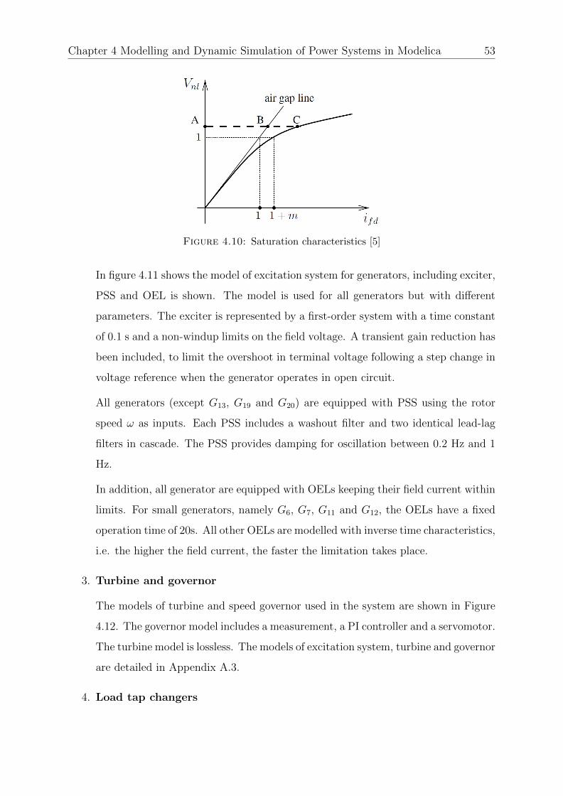
Chapter 4 Modelling and Dynamic Simulation of Power Systems in Modelica 53
Figure 4.10: Saturation characteristics [5]
In figure 4.11 shows the model of excitation system for generators, including exciter,
PSS and OEL is shown. The model is used for all generators but with different
parameters. The exciter is represented by a first-order system with a time constant
of 0.1 s and a non-windup limits on the field voltage. A transient gain reduction has
been included, to limit the overshoot in terminal voltage following a step change in
voltage reference when the generator operates in open circuit.
All generators (except G13, G19 and G20) are equipped with PSS using the rotor
speed ω as inputs. Each PSS includes a washout filter and two identical lead-lag
filters in cascade. The PSS provides damping for oscillation between 0.2 Hz and 1
Hz.
In addition, all generator are equipped with OELs keeping their field current within
limits. For small generators, namely G6, G7, G11 and G12, the OELs have a fixed
operation time of 20s. All other OELs are modelled with inverse time characteristics,
i.e. the higher the field current, the faster the limitation takes place.
3. Turbine and governor
The models of turbine and speed governor used in the system are shown in Figure
4.12. The governor model includes a measurement, a PI controller and a servomotor.
The turbine model is lossless. The models of excitation system, turbine and governor
are detailed in Appendix A.3.
4. Load tap changers
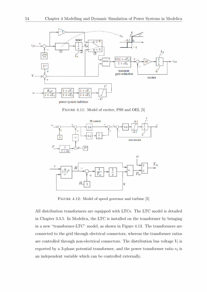
54 Chapter 4 Modelling and Dynamic Simulation of Power Systems in Modelica
Figure 4.11: Model of exciter, PSS and OEL [5]
Figure 4.12: Model of speed governor and turbine [5]
All distribution transformers are equipped with LTCs. The LTC model is detailed
in Chapter 3.3.5. In Modelica, the LTC is installed on the transformer by bringing
in a new “transformer-LTC” model, as shown in Figure 4.13. The transformers are
connected to the grid through electrical connectors, whereas the transformer ratios
are controlled through non-electrical connectors. The distribution bus voltage Vl is
exported by a 3-phase potential transformer, and the power transformer ratio rb is
an independent variable which can be controlled externally.

Chapter 4 Modelling and Dynamic Simulation of Power Systems in Modelica 55
The transformer-LTC model is connected with a LTC model in the manner shown
in Figure 4.14. Based on the value of Vl, LTC adjusts the transformer ratio to
control the distribution bus voltage.
Figure 4.13: Diagram and icon view of transformer-LTC model
Figure 4.14: Connection of LTC to the system model
4.4.3 Simulation and validation
To investigate dynamic response of the system, a three-phase short-circuit fault is applied
on “Bus2032” at t = 40 − 40.1s, with fault impedance Zfault = 0.0001 + j0.001. By
applying the fault on bus 2032, critical generators will not be affected seriously, and
dominant power flow will not be influenced.

56 Chapter 4 Modelling and Dynamic Simulation of Power Systems in Modelica
The system model validation is done by comparing responses of two systems from Dymola
and Simulink. The system response after fault is investigated by observing the following
outputs, as shown in Figure 4.15, 4.16 and 4.17:
• Distribution bus voltage: VB4022, VB4032 (NORTH) VB1044, VB1045 (CENTRAL)
• Generator terminal voltage: VG14, VG15 (CENTRAL)
• LTC operation: Transformer 1 connecting bus 1011 and load 1, transformer 17
connecting bus 4051 and load 51
0 10 20 30 40 50 60 70 800.9
0.92
0.94
0.96
0.98
1
1.02
1.04
1.06
Time [s]
v1044 [p,u
]
Bus 1044: voltage magnitude(p.u)
Simulink
Dymola
0 10 20 30 40 50 60 70 800.92
0.94
0.96
0.98
1
1.02
1.04
1.06
Time [s]
v1045 [p,u
]
Bus 1045: voltage magnitude(p.u)
Simulink
Dymola
0 10 20 30 40 50 60 70 800.88
0.9
0.92
0.94
0.96
0.98
1
1.02
Time [s]
v4022 [p,u
]
Bus 4022: voltage magnitude(p.u)
Simulink
Dymola
0 10 20 30 40 50 60 70 800.85
0.9
0.95
1
1.05
1.1
Time [s]
v4032 [p,u
]
Bus 4032: voltage magnitude(p.u)
Simulink
Dymola
Figure 4.15: Distribution bus voltages in IEEE Nordic 32 system
0 10 20 30 40 50 60 70 800.95
1
1.05
1.1
Time [s]
vg14 [p,u
]
Generator 14: terminal voltage magnitude(p.u)
Simulink
Dymola
0 10 20 30 40 50 60 70 800.95
1
1.05
1.1
Time [s]
vg15 [p
,u]
Generator 15: terminal voltage magnitude(p.u)
Simulink
Dymola
Figure 4.16: Generator terminal voltages in IEEE Nordic 32 system
Discussion: As shown by distribution bus voltages in Figure 4.17, in response to the
distribution applied on bus 2032 at t = 40 − 40.1s, the system exhibits damped elec-
tromechanical oscillations that die out in 15 seconds. Since the fault is applied in North
area, the voltages in Central buses are less influenced than Northern buses.

Chapter 4 Modelling and Dynamic Simulation of Power Systems in Modelica 57
25 30 35 40 45 50 55 60 65 70 75
0.94
0.95
0.96
0.97
0.98
0.99
1
1.01
1.02
1.03
Time [s]
Transmission bus 1011: voltage magnitude (pu)
Distribution bus 11: voltage magnitude (pu)
Branch 1: magnitide of transformer ratio
30 35 40 45 50 55 60 65 70 75 80
0.96
0.98
1
1.02
1.04
1.06
1.08
Time [s]
Transmission bus 4051: voltage magnitude (pu)
Distribution bus 51: voltage magnitude (pu)
Branch 17: magnitide of transformer ratio
Figure 4.17: LTC operations in IEEE Nordic 32 system
In Figure 4.16, generator terminal voltages are controlled to keep constant. Compared
with the generator terminal voltages of KTH Nordic 32 system shown in Figure 4.8, it
can be found that when the same disturbance is applied on Nordic 32 system, although
generators are equipped with different excitation system and governor models, effects of
the control are similar.
In addition, from the comparison between the outputs from two systems in Dymola and
Simulnk, it can be seen that two systems response to the disturbance in a fairy similar
way. The small deviations between the oscillation processes are caused by the differences
between numerical solvers in two softwares.
Consideration of LTC operations is a major difference between KTH Nordic 32 and IEEE
Nordic 32 system. To present the effect of LTC operations, the dynamics of transformer
ratio and distribution bus voltage are shown in Figure 4.17. The figures show the success-
ful attempt of LTC to bring distribution voltages back within the [0.99, 1.01] deadband.
The solid and dashed lines in the figure are distribution and transmission bus voltages
respectively. As seen in the figure, when distribution bus voltage is above the limitation,
LTC will keep changing the transformer ratio after a certain delay, until distribution bus
voltage is within the acceptable range.

58 Chapter 4 Modelling and Dynamic Simulation of Power Systems in Modelica
4.5 iGrGen - Greece Generator system
4.5.1 System overview
The Greece generator system is a Combined Cycle Power Plant (CCPP). The power plant
consists of a gas turbine, a steam turbine and a synchronous generator on a single shaft
arrangement. The one-line diagram of iGrGen system is shown in Figure 4.18.
Figure 4.18: One-line diagram of iGrGen system
As the figure shows, the step–up transformer (STEP UP TR) connects the generator to
the 400 kV busbar (HV BUS) with a overhead transmission line. The system also includes
auxiliary loads (medium voltage motors), which are connected to the 6.6 kV busbar (MV
BUS). The auxiliary load bus connects to the generator with an auxiliary transformer
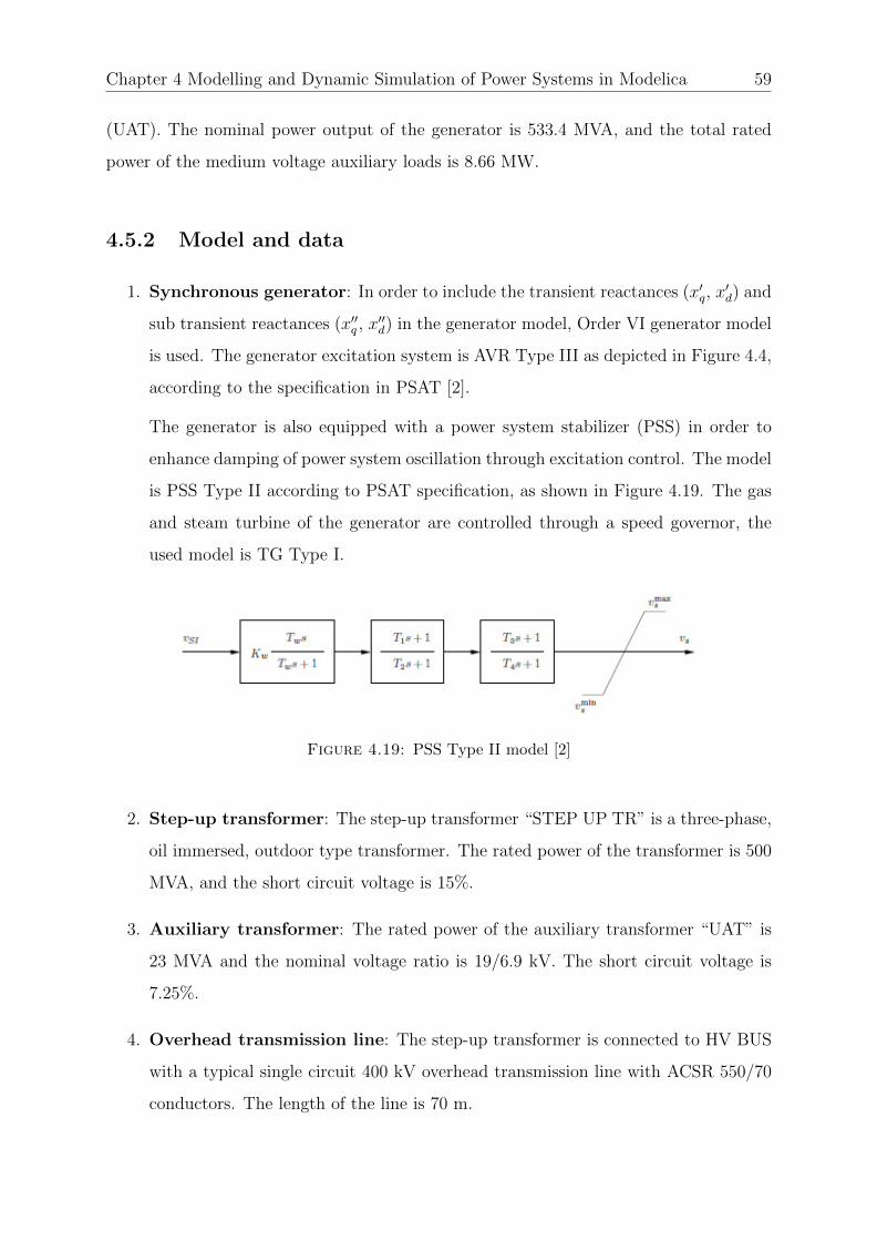
Chapter 4 Modelling and Dynamic Simulation of Power Systems in Modelica 59
(UAT). The nominal power output of the generator is 533.4 MVA, and the total rated
power of the medium voltage auxiliary loads is 8.66 MW.
4.5.2 Model and data
1. Synchronous generator: In order to include the transient reactances (x′q, x′d) and
sub transient reactances (x′′q , x′′d) in the generator model, Order VI generator model
is used. The generator excitation system is AVR Type III as depicted in Figure 4.4,
according to the specification in PSAT [2].
The generator is also equipped with a power system stabilizer (PSS) in order to
enhance damping of power system oscillation through excitation control. The model
is PSS Type II according to PSAT specification, as shown in Figure 4.19. The gas
and steam turbine of the generator are controlled through a speed governor, the
used model is TG Type I.
Figure 4.19: PSS Type II model [2]
2. Step-up transformer: The step-up transformer “STEP UP TR” is a three-phase,
oil immersed, outdoor type transformer. The rated power of the transformer is 500
MVA, and the short circuit voltage is 15%.
3. Auxiliary transformer: The rated power of the auxiliary transformer “UAT” is
23 MVA and the nominal voltage ratio is 19/6.9 kV. The short circuit voltage is
7.25%.
4. Overhead transmission line: The step-up transformer is connected to HV BUS
with a typical single circuit 400 kV overhead transmission line with ACSR 550/70
conductors. The length of the line is 70 m.
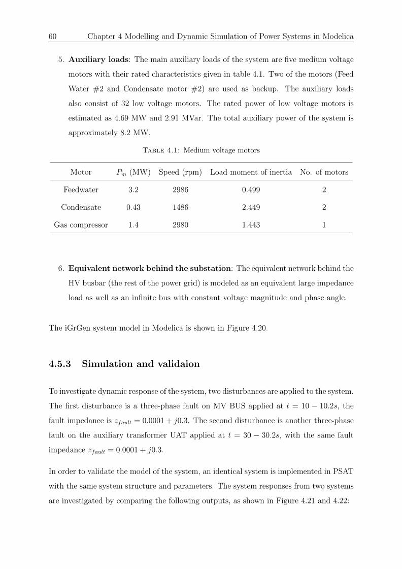
60 Chapter 4 Modelling and Dynamic Simulation of Power Systems in Modelica
5. Auxiliary loads: The main auxiliary loads of the system are five medium voltage
motors with their rated characteristics given in table 4.1. Two of the motors (Feed
Water #2 and Condensate motor #2) are used as backup. The auxiliary loads
also consist of 32 low voltage motors. The rated power of low voltage motors is
estimated as 4.69 MW and 2.91 MVar. The total auxiliary power of the system is
approximately 8.2 MW.
Table 4.1: Medium voltage motors
Motor Pm (MW) Speed (rpm) Load moment of inertia No. of motors
Feedwater 3.2 2986 0.499 2
Condensate 0.43 1486 2.449 2
Gas compressor 1.4 2980 1.443 1
6. Equivalent network behind the substation: The equivalent network behind the
HV busbar (the rest of the power grid) is modeled as an equivalent large impedance
load as well as an infinite bus with constant voltage magnitude and phase angle.
The iGrGen system model in Modelica is shown in Figure 4.20.
4.5.3 Simulation and validaion
To investigate dynamic response of the system, two disturbances are applied to the system.
The first disturbance is a three-phase fault on MV BUS applied at t = 10 − 10.2s, the
fault impedance is zfault = 0.0001 + j0.3. The second disturbance is another three-phase
fault on the auxiliary transformer UAT applied at t = 30 − 30.2s, with the same fault
impedance zfault = 0.0001 + j0.3.
In order to validate the model of the system, an identical system is implemented in PSAT
with the same system structure and parameters. The system responses from two systems
are investigated by comparing the following outputs, as shown in Figure 4.21 and 4.22:
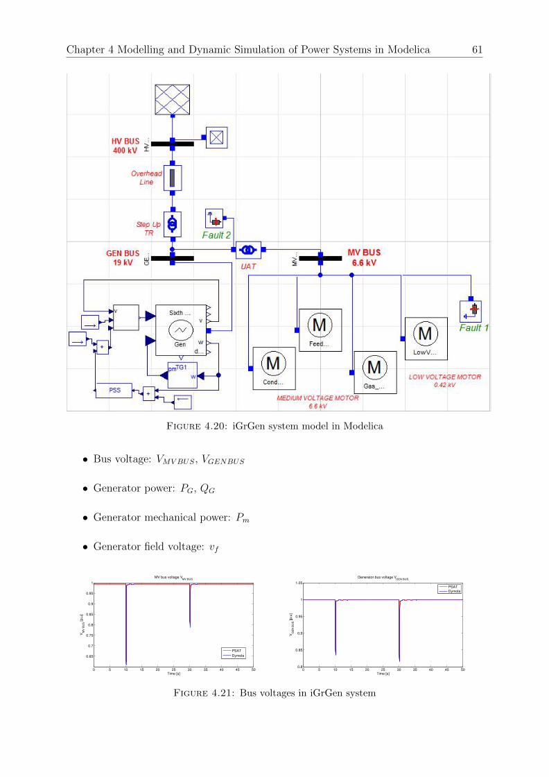
Chapter 4 Modelling and Dynamic Simulation of Power Systems in Modelica 61
Figure 4.20: iGrGen system model in Modelica
• Bus voltage: VMVBUS, VGENBUS
• Generator power: PG, QG
• Generator mechanical power: Pm
• Generator field voltage: vf
0 5 10 15 20 25 30 35 40 45 50
0.65
0.7
0.75
0.8
0.85
0.9
0.95
1
Time [s]
VM
V B
US [p,u
]
MV bus voltage VMV BUS
PSAT
Dymola
0 5 10 15 20 25 30 35 40 45 500.8
0.85
0.9
0.95
1
1.05
Time [s]
VG
EN
BU
S [p,u
]
Generator bus voltage VGEN BUS
PSAT
Dymola
Figure 4.21: Bus voltages in iGrGen system
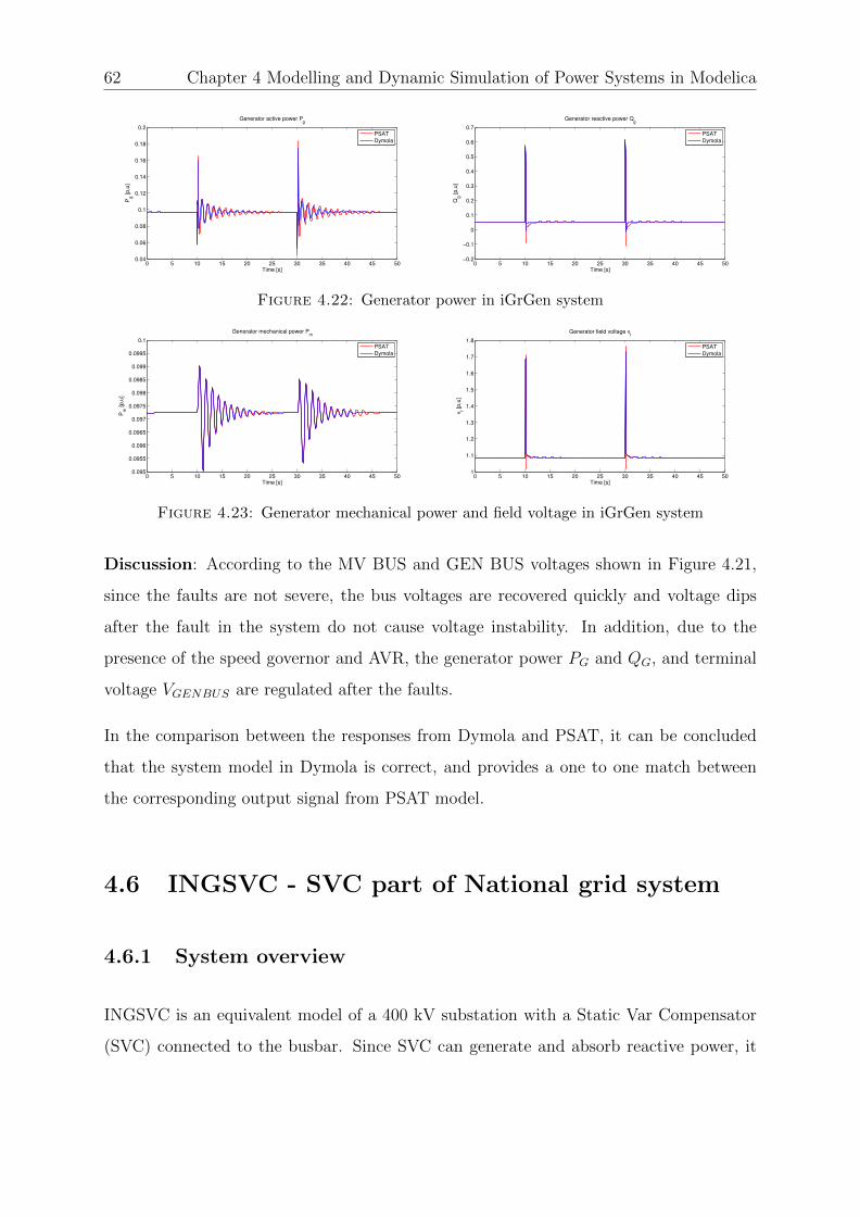
62 Chapter 4 Modelling and Dynamic Simulation of Power Systems in Modelica
0 5 10 15 20 25 30 35 40 45 500.04
0.06
0.08
0.1
0.12
0.14
0.16
0.18
0.2
Time [s]
Pg [p,u
]
Generator active power Pg
PSAT
Dymola
0 5 10 15 20 25 30 35 40 45 50−0.2
−0.1
0
0.1
0.2
0.3
0.4
0.5
0.6
0.7
Time [s]
Qg [p,u
]
Generator reactive power Qg
PSAT
Dymola
Figure 4.22: Generator power in iGrGen system
0 5 10 15 20 25 30 35 40 45 500.095
0.0955
0.096
0.0965
0.097
0.0975
0.098
0.0985
0.099
0.0995
0.1
Time [s]
Pm
[p,u
]
Generator mechanical power Pm
PSAT
Dymola
0 5 10 15 20 25 30 35 40 45 501
1.1
1.2
1.3
1.4
1.5
1.6
1.7
1.8
Time [s]
vf [
p,u
]
Generator field voltage vf
PSAT
Dymola
Figure 4.23: Generator mechanical power and field voltage in iGrGen system
Discussion: According to the MV BUS and GEN BUS voltages shown in Figure 4.21,
since the faults are not severe, the bus voltages are recovered quickly and voltage dips
after the fault in the system do not cause voltage instability. In addition, due to the
presence of the speed governor and AVR, the generator power PG and QG, and terminal
voltage VGENBUS are regulated after the faults.
In the comparison between the responses from Dymola and PSAT, it can be concluded
that the system model in Dymola is correct, and provides a one to one match between
the corresponding output signal from PSAT model.
4.6 INGSVC - SVC part of National grid system
4.6.1 System overview
INGSVC is an equivalent model of a 400 kV substation with a Static Var Compensator
(SVC) connected to the busbar. Since SVC can generate and absorb reactive power, it
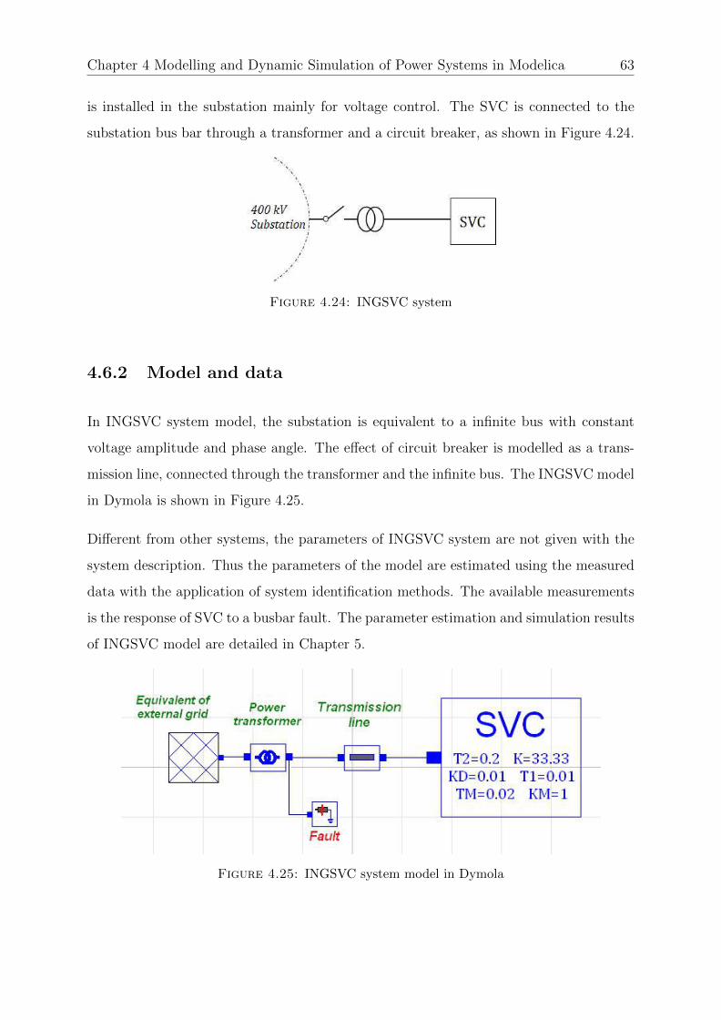
Chapter 4 Modelling and Dynamic Simulation of Power Systems in Modelica 63
is installed in the substation mainly for voltage control. The SVC is connected to the
substation bus bar through a transformer and a circuit breaker, as shown in Figure 4.24.
Figure 4.24: INGSVC system
4.6.2 Model and data
In INGSVC system model, the substation is equivalent to a infinite bus with constant
voltage amplitude and phase angle. The effect of circuit breaker is modelled as a trans-
mission line, connected through the transformer and the infinite bus. The INGSVC model
in Dymola is shown in Figure 4.25.
Different from other systems, the parameters of INGSVC system are not given with the
system description. Thus the parameters of the model are estimated using the measured
data with the application of system identification methods. The available measurements
is the response of SVC to a busbar fault. The parameter estimation and simulation results
of INGSVC model are detailed in Chapter 5.
Figure 4.25: INGSVC system model in Dymola

Chapter 5
System identification
5.1 Introduction
System identification is a number of methods to build valid mathematical models for
a dynamic system based on measurement data [37]. Particularly, a system model is
identified by estimating and adjusting parameters until its outputs match the measured
outputs with acceptable error.
System identification is an important task in power system modelling and simulation. The
system model may have been developed with a reference component, and the validity of
such model is directly linked to the fidelity of the parametrization. In most cases, the
parameters are not given with a system model; even for the models with parameters,
the available parameters may not correspond to real values due to several reasons: the
model may have been validated against a different component; the parameter value have
changed over time, etc. [8].
In this chapter, experience of power system identification is provided with the aid of iTesla
RaPID toolbox developed by SmarTS Lab. Two system models are identified against
measurement data: the Greece generator system iGrGen, and the National Grid SVC
system INGSVC. Since system identification requires different computational methods,
two kinds of optimization algorithms are used, and the obtained results are analysed
65
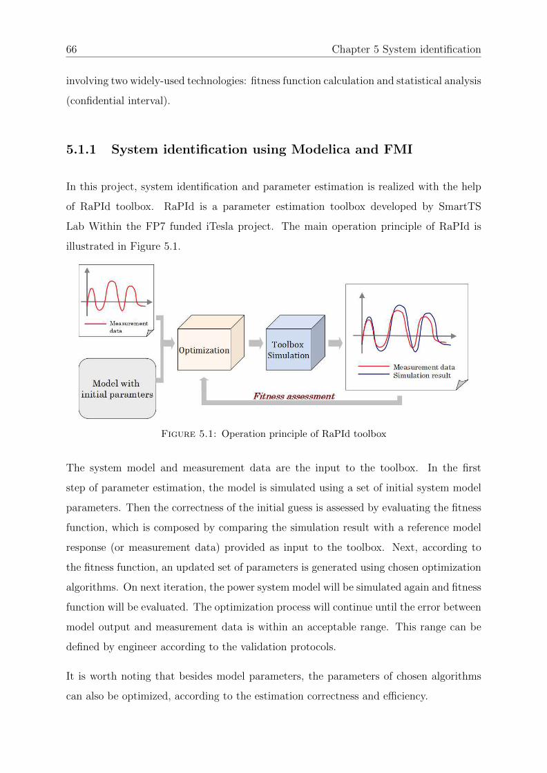
66 Chapter 5 System identification
involving two widely-used technologies: fitness function calculation and statistical analysis
(confidential interval).
5.1.1 System identification using Modelica and FMI
In this project, system identification and parameter estimation is realized with the help
of RaPId toolbox. RaPId is a parameter estimation toolbox developed by SmartTS
Lab Within the FP7 funded iTesla project. The main operation principle of RaPId is
illustrated in Figure 5.1.
Figure 5.1: Operation principle of RaPId toolbox
The system model and measurement data are the input to the toolbox. In the first
step of parameter estimation, the model is simulated using a set of initial system model
parameters. Then the correctness of the initial guess is assessed by evaluating the fitness
function, which is composed by comparing the simulation result with a reference model
response (or measurement data) provided as input to the toolbox. Next, according to
the fitness function, an updated set of parameters is generated using chosen optimization
algorithms. On next iteration, the power system model will be simulated again and fitness
function will be evaluated. The optimization process will continue until the error between
model output and measurement data is within an acceptable range. This range can be
defined by engineer according to the validation protocols.
It is worth noting that besides model parameters, the parameters of chosen algorithms
can also be optimized, according to the estimation correctness and efficiency.

Chapter 5 System identification 67
The RaPId toolbox is developed in MATLAB. The top-level MATLAB code acts as a
wrapper to provide interaction with several other tools [38]. The interaction of the tools
are realized in the following pattern:
• MATLAB: MATLAB combines all the software to realize the toolbox’s simulation
and optimization functions. It provides a Graphical User Interface (GUI) and a
Command Line Interface (CLI) for the user of the toolbox. Built-in parameter
optimization algorithms are also developed in MATLAB, and several MATLAB
toolboxes are used within RAPID toolbox.
• Simulink: Simulink is used to configure the models used by RAPId, and generate
simulation results used by RaPId toolbox for fitness assessment.
• Modelica: The system model is developed and identified in Modelica language.
• FMU: System model is compiled into a Flexible Mock-up Unit (FMU) according
to the FMI standard. FMU is a C-object containing the methods for simulation.
FMU is used as input to RaPId toolbox.
5.1.2 Optimization algorithms
To find the parameters which minimize the error between the measurement data and the
simulation results, different optimization algorithms are used in the parameter estimation
showed in Figure 5.1. There are six algorithms integrated in RaPId toolbox in total,
among which the following two algorithms are applied for the parameter estimation in
this thesis:
• Particle swarm optimization algorithm: The PSO method is a meta-heuristic
algorithm for global random optimization. No prior assumptions are made in this
algorithm and it can search in a large space of candidate solutions, thus it is not
guaranteed that the optimal solution can be found [39].
The algorithm works by having a group of candidate solutions (normally called
particles). At the beginning these particles are distributed randomly around the
68 Chapter 5 System identification
solution space, in each position the particle evaluates its own fitness. In every
iteration, the particle changes its position according some criteria, according to the
algorithm implementation.
• Particle filter algorithm: Particle filter algorithm is a posterior density estima-
tion algorithm that estimate the posterior density of the state-space by directly
implementing the Bayesian recursion estimation equations. Recursive Bayesian es-
timation is a general probabilistic approach for estimation unknown probability
density function recursively over time using incoming measurements and a mathe-
matical process model [40]. The advantage of the algorithm is that it performs well
in finding global solutions.
5.1.3 Power system parameter estimation
In this section, the specified steps used to identify parameters of power system using
RaPId toolbox is presented. The main steps in this process are the following:
1. Collect measurement data
2. Implement power system model using Modelica language
3. Compile the Modelica model into FMU format
4. Create a Simulink model, load the previously complied Modelica model into the
Simulink model using the FMI toolbox for MATLAB
5. Start the RaPId Toolbox, and input the settings required by the toolbox (inputs,
outputs, algorithm, parameters, etc.)
6. Run the parameter identification algorithms
7. Evaluate the results of identification
Collect measurement data

Chapter 5 System identification 69
The measurement data in this contest is a recorded output from the real world or a
reference system. Collection of measurement data can be connected with the difficulties
of the power system components stage tests. In the case of reference model, experiments
set up and the measurement data collection is simpler and gives flexibility to the engineer.
In most cases the measurement data needs to pass through pre-processing before it can
be used as input for the system identification. The reason for that is the presence of
noise, and unnecessary data which does not characterized by parameters to be estimated.
Implement Modelica models, and compile it into FMU format
In this thesis the language chosen for power system identification is Modelica (as it
was mentioned and shown below in Figure 4.20 and 4.25). In Dymola, the Modelica
models can be compiled into FMUs. The RaPId toolbox utilizes the compiled FMU as
the mathematical model with parameters to be estimated of real system via the FMI
toolbox for Matlab. The FMU is compliant with the FMI standard (Functional Mock-up
interface), which is a tool independent standard for the exchange of dynamic models and
for co-Simulation [41].
When compiling FMU, two kinds of FMU can be chosen:
• FMU for model exchange: generates lime C-Code or object code containing the
dynamic system model in the form of blocks with input and output.
• FMU for co-simulation: similar to FMU for model exchange, but contains the solvers
together with the model.
To simulate the model using the solvers provided by MATLAB/Simulink, FMU for model
exchange is used.
Create a Simulink model and load the previously complied Modelica model
Simulink model is used as an interface for loading and configuring parameters in the model
via FMI toolbox for MATLAB. Additional Simulink components are also used to serve as
a link between FMU and RaPId toolbox. For instance, from workspace and to workspace
are utilized for monitoring the measurement data, and redirecting the simulation results
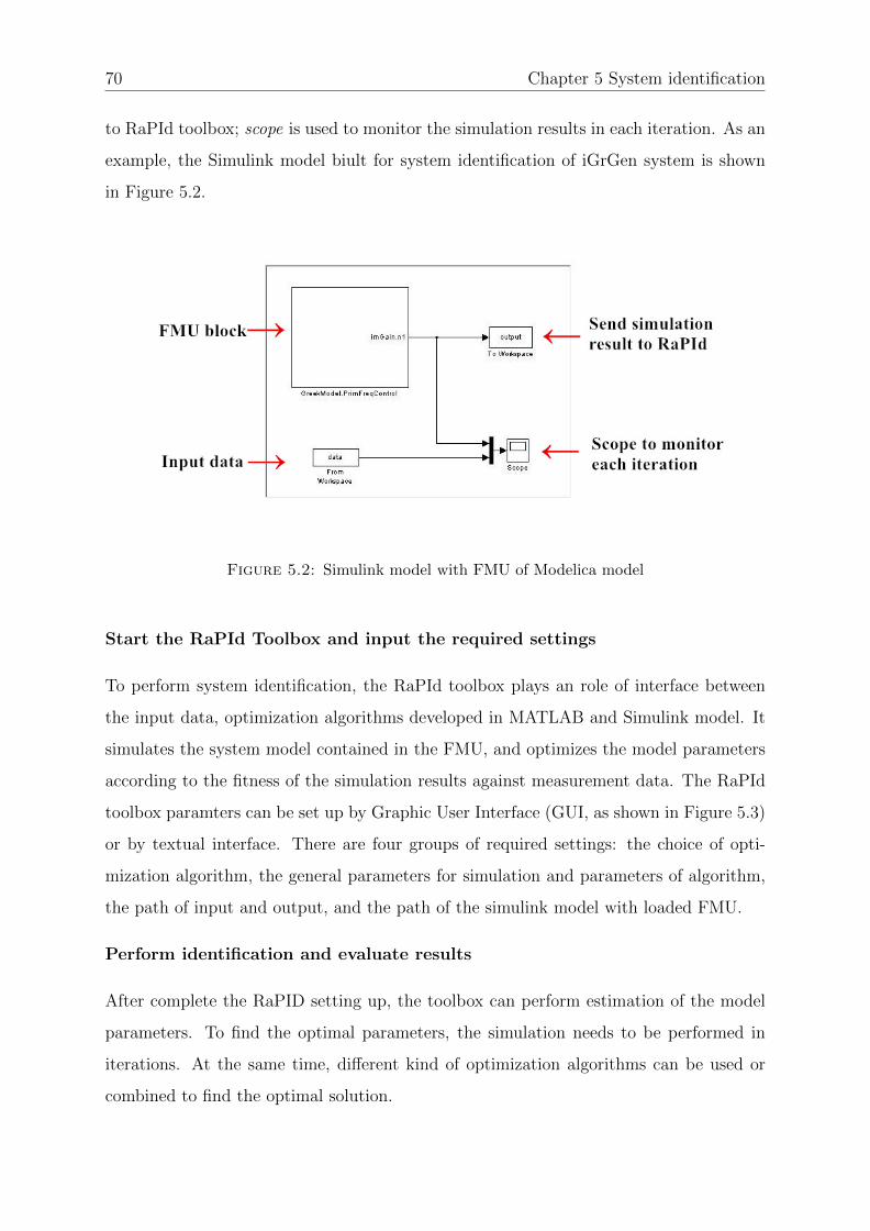
70 Chapter 5 System identification
to RaPId toolbox; scope is used to monitor the simulation results in each iteration. As an
example, the Simulink model biult for system identification of iGrGen system is shown
in Figure 5.2.
Figure 5.2: Simulink model with FMU of Modelica model
Start the RaPId Toolbox and input the required settings
To perform system identification, the RaPId toolbox plays an role of interface between
the input data, optimization algorithms developed in MATLAB and Simulink model. It
simulates the system model contained in the FMU, and optimizes the model parameters
according to the fitness of the simulation results against measurement data. The RaPId
toolbox paramters can be set up by Graphic User Interface (GUI, as shown in Figure 5.3)
or by textual interface. There are four groups of required settings: the choice of opti-
mization algorithm, the general parameters for simulation and parameters of algorithm,
the path of input and output, and the path of the simulink model with loaded FMU.
Perform identification and evaluate results
After complete the RaPID setting up, the toolbox can perform estimation of the model
parameters. To find the optimal parameters, the simulation needs to be performed in
iterations. At the same time, different kind of optimization algorithms can be used or
combined to find the optimal solution.

Chapter 5 System identification 71
Figure 5.3: Main GUI of RaPId toolbox
5.2 Parameter estimation case 1: Turbine parame-
ters of iGrGen system model
The Greece generator system iGrGen is a Combined Cycle Power Plant containing a gas
turbine, a steam turbine and a synchronous generator in a single shaft arrangement. A
speed governor is used in gas turbine to control the system frequency. The iGrGen system
is detailed in Chapter 4.5.1.
5.2.1 Experiment set-up
Measurement data
The measurement data used for system identification is obtained from experiments per-
formed on the gas turbine governor. The purpose of the experiment is to demonstrate
the response of generator turbine to system frequency deviation, thus the measured data
is the turbine mechanical power output. If the system frequency decreases below rated
frequency, the turbine will be controlled to increase the output mechanical power; if the

72 Chapter 5 System identification
system frequency increases above the rated frequency, the turbine will reduce the power
output.
It worth noting that the steam turbine in the power plant does not contribute initially
to the primary frequency control because of the large thermal inertia.
Modelica model
The Modelica model of iGrGen system is shown in Figure 5.4. Incremental signal is
injected to the frequency reference input of the governor to simulate the effect of variation
of system frequency. The injected signals are in forms shown in Figure 5.5, with the
frequency deviation ∆ω = +/− 0.2Hz (0.004p.u).
Figure 5.4: Modelica model of iGrGen system for system identification
Parameter estimation
The Simulink model with compiled FMU from the Modelica model is shown in Figure
5.2. Two kinds of algorithms are selected to find the optimal parameters: particle swarm
optimization (PSO) algorithm and particle filters (PF) algorithm. The parameters to be
estimated are listed in Table 5.1.

Chapter 5 System identification 73
Figure 5.5: Injected signals to the system
Table 5.1: Parameters to be estimated
Parameter Parameter
R Droop Ts Governor time constant
Tc Servo time constant T3 Transient time constant
T4 Power fraction time constant T5 Reheat time constant
5.2.2 Results
The numerical results of the generator parameter estimation process are shown in Table
5.2. Two kinds of optimization algorithm are used, and the performances are evaluated
by comparing the mean squared error (MSE) and convergence time.
Table 5.2: Parameter estimation results
Algorithm Parameter Value Parameter Value Time (s) MSE
PSO R 0.3201 Ts 15.5085 189.999 4.7332
+Gradient descent Tc 0.3 T3 0.04
T4 5 T5 4
PF R 0.3145 Ts 15.8765 61.799 4.4792
+Gradient descent Tc 0.3 T3 0.04
T4 5 T5 4
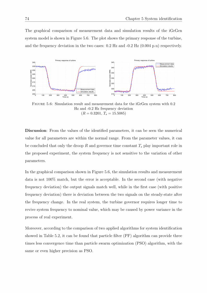
74 Chapter 5 System identification
The graphical comparison of measurement data and simulation results of the iGrGen
system model is shown in Figure 5.6. The plot shows the primary response of the turbine,
and the frequency deviation in the two cases: 0.2 Hz and -0.2 Hz (0.004 p.u) respectively.
0 100 200 300 400 500 600 700 800200
205
210
215
220
225
230
235
240
Time (s)
Ge
ne
rato
r p
ow
er
(MW
)
Primary response of turbine
Measurement data
Simulation results
0 100 200 300 400 500 600 700 800315
320
325
330
335
340
345
Time (s)
Genera
tor
pow
er
(MW
)
Primary response of turbine
Measurement data
Simulation results
Figure 5.6: Simulation result and measurement data for the iGrGen system with 0.2Hz and -0.2 Hz frequency deviation
(R = 0.3201, Ts = 15.5085)
Discussion: From the values of the identified parameters, it can be seen the numerical
value for all parameters are within the normal range. From the parameter values, it can
be concluded that only the droop R and governor time constant Ts play important role in
the proposed experiment, the system frequency is not sensitive to the variation of other
parameters.
In the graphical comparison shown in Figure 5.6, the simulation results and measurement
data is not 100% match, but the error is acceptable. In the second case (with negative
frequency deviation) the output signals match well, while in the first case (with positive
frequency deviation) there is deviation between the two signals on the steady-state after
the frequency change. In the real system, the turbine governor requires longer time to
revive system frequency to nominal value, which may be caused by power variance in the
process of real experiment.
Moreover, according to the comparison of two applied algorithms for system identification
showed in Table 5.2, it can be found that particle filter (PF) algorithm can provide three
times less convergence time than particle swarm optimization (PSO) algorithm, with the
same or even higher precision as PSO.

Chapter 5 System identification 75
5.3 Parameter estimation case 2: SVC parameters
of INGSVC system model
INGSVC is an equivalent model of a 400 kV substation with a Static Var Compensator
(SVC) connected to the busbar. The substation is modelled as an infinite bus, and the
SVC model is connected to the bus with a transmission line and a transformer. The
system is detailed in Chapter 4.6.1.
5.3.1 Experiment set-up
Measurement data
The measurement data used for system identification is obtained from experiment per-
formed on the substation. In the experiment, a fault is applied on the substation busbar.
The purpose of the experiment is to demonstrate the response of SVC to the fault, thus
the measured data is the voltage and current on the terminal of SVC.
Modelica model
The Modelica model of the INGSVC system is shown in Figure 4.25. To simulate the
effect of busbar fault, a fault is applied to the second side of transformer, leading to a
voltage dip in the SVC terminal.
Parameter estimation
The Simulink model with compiled FMU from the Modelica model is shown in Figure 5.7.
Similiar to case 1, particle swarm optimization algorithm and particle filters algorithm
are selected to find the optimal parameters. The parameters to be estimated are listed
in Table 5.1.
5.3.2 Results
The numerical results of the generator parameter estimation are shown in Table 5.4.
Similar to case 1, two kinds of optimization algorithm are applied and compared. The
graphical comparison of measurement data and simulation results of the INGSVC system

76 Chapter 5 System identification
Figure 5.7: Simulink model with FMU of INGSVC system Modelica model
Table 5.3: Parameters to be estimated
Parameter Parameter
α0 SVC firing angle K Regulator gain
KD Integral deviation T2 Regulator time constant
T1 Transient regulator time constant Tm Measure time delay
Km Measure Gain xl Reactance (inductive)
xc Reactance(capacitive)
model is shown in Figure 5.8. The plots show the voltage and current responses of SVC
to the fault applied on the substation busbar respectively.
In this case, other than the fitness indicated by MSE, another performance indicator:
statistical analysis is used to evaluate the validity of identification results with the help
of MATLAB statistics toolbox. From the results listed in Table 5.4, it can be found the
main differences between two groups of parameters are the value of SVC firing angle α0
and regulator gain K. To find the optimal value for the two parameters, the estimation
is performed for 30 times with particle filter algorithm. The statistical analysis of the
results is shown in Figure 5.9.

Chapter 5 System identification 77
Table 5.4: Parameter estimation results
Algorithm Parameter Value Parameter Value Time (s) MSE
PSO α0 0.2012 K 33.3301 256.988 7.128× 10⁻⁴
+Gradient descent KD 0.01 T2 0.2
T1 0.01 Tm 0.02
Km 1 xl 0.2
xc 0.1
PF α0 0.2030 K 32.9301 155.442 6.228× 10⁻⁴
+Gradient descent KD 0.01 T2 0.2
T1 0.01 Tm 0.02
Km 1 xl 0.2
xc 0.1
0 0.1 0.2 0.3 0.4 0.5 0.6 0.70.7
0.75
0.8
0.85
0.9
0.95
1
1.05
1.1
Time (s)
Voltage (
p.u
)
Response of SVC to voltage dip
Measurement data
Simulation results
0 0.1 0.2 0.3 0.4 0.5 0.6 0.7−0.5
0
0.5
1
1.5
2
Time (s)
Curr
ent (p
.u)
Response of SVC to voltage dip
Measurement data
Simulation results
Figure 5.8: Simulation result and measurement data for the INGSVC system(α0 = 0.2012, K = 33.3301)
Discussion: From the numerical results of system identification, it can be found the
values of the identified parameters are within the normal range. Apparently only the
values of SVC firing angle α0 and regulator gain K influence the SVC’s response to the
applied busbar fault.
In the graphical comparison shown in Figure 5.8, it can be seen that the simulation result
and measurement data of SVC terminal voltage match well, but there exists large error
between simulation and measurements in SVC terminal current. The reason are two-
fold: first of all, the test system is a rough approximation of the real system; and many

78 Chapter 5 System identification
Statistics of α0 Statistics of K
• Mean value μ : 0.2030• Variance σ : 0.0122• 95% confidence interval: [0.1985, 0.2076]
• Mean value μ : 32.9301• Variance σ : 0.7346• 95% confidence interval: [32.6558, 33.2044]
Figure 5.9: Statistical analysis for parameter estimation results
simplifications are made in the modelling of the SVC model, which may not respond to
the system disturbance as a real component. Because of the simplifications, the SVC
model may response to the fault in form of instantaneous current changes other than
oscillations, as shown in the left plot in Figure 5.8. Nevertheless, the model and the
estimated parameters can still be used to investigate the effect of SVC on the overall
system operation.
From the statistical analysis results presented in Figure 5.9, the confidence interval for α0
is from 0.1985 to 0.2076, while for K the confidence interval is from 32.6558 to 32.2044.
Figure 5.10 and 5.11 present the graphical comparisons of simulation results and measure-
ment data with α0 = 0.1985, K = 33.2044 and α0 = 0.2076, K = 32.6558 respectively.
By comparing the two groups of plots with different parameter values, it is observed that
although the parameter values are at the edges of confidence interval, there exists no large
deviation between the two cases, and the case shown in Figure 5.8. Thus the conclusion
can be derived that any parameter value in the confidence interval is acceptable and can
be applied on the model.
Similarly to case 1, according to the comparison of algorithms presensed in Table 5.4, it
can also be concluded that particle filter (PF) algorithm perform faster with the same or

Chapter 5 System identification 79
0 0.1 0.2 0.3 0.4 0.5 0.6 0.70.7
0.75
0.8
0.85
0.9
0.95
1
1.05
1.1
Time (s)
Voltage (
p.u
)Response of SVC to voltage dip
Measurement data
Simulation results
0 0.1 0.2 0.3 0.4 0.5 0.6 0.7−0.5
0
0.5
1
1.5
2
Time (s)
Curr
ent (p
.u)
Response of SVC to voltage dip
Measurement data
Simulation results
Figure 5.10: Simulation result and measurement data for the INGSVC system(α0 = 0.1985, K = 33.2044)
0 0.1 0.2 0.3 0.4 0.5 0.6 0.70.7
0.75
0.8
0.85
0.9
0.95
1
1.05
1.1
Time (s)
Voltage (
p.u
)
Response of SVC to voltage dip
Measurement data
Simulation results
0 0.1 0.2 0.3 0.4 0.5 0.6 0.7−0.5
0
0.5
1
1.5
2
Time (s)
Curr
ent (p
.u)
Response of SVC to voltage dip
Measurement data
Simulation results
Figure 5.11: Simulation result and measurement data for the INGSVC system(α0 = 0.2076, K = 32.6558)
higher precision as particle swarm optimization (PSO) algorithm.

Chapter 6
Discussion
6.1 Modelica
In chapter 3 and 4, the experience of Modelica based power system modelling, simula-
tion and validation are presented. In general, Modelica is advantageous compared with
other modelling tools mainly in four aspects. First of all, it allows the implementation of
high complexity models using simple mathematical language; secondly, model exchange
between software environments and co-simulation is possible in Modelica; thirdly, the
powerful mathematical solvers integrated in the Modelica simulation environments pro-
vides the user the freedom to select the optimal method to solve very complex systems;
finally, as the validation results presented in chapter 3 and 4 show, Modelica has been
proven to achieve identical results of other power system analysis specific tools, provided
new extra features.
6.1.1 Modelling, simulation and validation of system compo-
nents
Sixteen power system component models are developed in Modelica in this thesis. Since
the validation results in chapter 3 and appendix A are positive, the potential of achieving
accurate modelling of Modelica is proven. Considering the components modelled in this
81
82 Chapter 6 Discussion
thesis are mainly control elements, it is feasible to implement more complex power system
models in Modelica.
Modelica also provides sufficient flexibility in power system modelling. The model can be
described not only by mathematical equations, also by connecting other existing models.
In addition, even though the models developed in this thesis are originally implemented
in different software environments with different properties, Modelica is able to represent
all necessary characteristics correctly in one single model.
6.1.2 Modelling and simulation of power systems
Chapter 4 presents the models and simulation results of four systems of different scale.
The system models are validated against the reference models with satisfying results,
which provides the possibilities of doing power system analysis, especially dynamic sim-
ulation in Modelica simulation environments.
Compared with other software tools, Modelica is advantageous for it simplifies the mod-
elling process of power systems. Users can develop specific models and libraries according
to the system characteristics, thus the problem of “lack of suitable models” in other soft-
ware is no longer a restriction. Modelica also provides users the freedom to decide which
solver to use in order to obtain the best results and the shortest simulation time.
Considering the limitation of Modelica in power system modelling, it is found that the
simulation time will increase on a large scale with the model size and number of variables
and equations. Therefore in order to achieve high simulation efficiency, the approaches of
model reduction and simplification need to be investigated when implement large scale
power system models in Modelica.
6.1.3 Model exchange
Chapter 5 shows the experience of system identification using the model exchange function
provided by Modelica. In this point of view, Modelica is not only a modelling language,
but also provides possibilities of re-utilization and sharing. The fact that any Modelica

Chapter 6 Discussion 83
model can be converted to an FMU and then be able to run in different software envi-
ronment is a revolution. With the help of Modelica, the process of software-to-software
modelling and validation can be simplified on a large scale.
As stated in chapter 1, the power systems simulation and analysis tools are commonly
incompatible. For instance, a model developed in PowerFactory cannot be used in PSAT.
This fact will cause problem when organizations using different tools need to collaborate,
and will finally lead to economic losses. The results shown in chapter 5 can be seen as
an evidence to solve this problem using Modelica.
6.2 System identification with RaPId toolbox
In chapter 5, system identification and parameter estimation are performed in MATLAB
environment with the help of RaPId toolbox. Two system models are identified with
estimated parameters, and the simulation results can match measured data well. RaPId
toolbox thus can be proven to be a very powerful tool to perform system identification,
provided many optimization algorithms and the convenience to use.
However in the identification process, it can be found that the level of noise in measure-
ment data will effect the convergence time and result accuracy to a large extent. For the
measurements obtained from real experiments with high level of noise, it is hard for the
toolbox to find optimal solution. Therefore, some signal processing methods are necessary
to be integrated to the toolbox.
In the identification process, the results are evaluated according to two kinds of perfor-
mance indicators: the best fitness of simulation results and measurement data (mean
squared error), and statistical analysis. The best fitness method is faster and easier to
evaluate the results, but statistical analysis can provide more information about validity
of the results. In general, no matter which evaluation methods is used, it will be beneficial
to perform the parameter estimation for several times to find the optimal solution.

Chapter 7
Conclusion and future work
7.1 Conclusions
This thesis provides a proof of the priority of a equation-based and object-oriented mod-
elling language, Modelica, on the field of electric power system modelling, simulation and
validation. The modelling and validation of power system components are successful.
The success is a foundation for the future work of more complex power system modelling
and simulation.
This thesis also proves the feasibility of implementing power system models, thereby doing
dynamic simulation and other relevant power system analysis in Modelica-based simula-
tion environment. Modelica allows users to develop specific model libraries according to
the system characteristics, and the powerful mathematical solvers integrated in Modelica
tools also provide the possibility to solve the problem more efficiently and accurately for
complex and large power system models.
The measurement-based system identification task in this thesis not only presents an
application of high-accuracy parameter estimation, but also a success in model exchanging
and the usage of the FMI standard. This function provided by Modelica has a lot of
potential and can be further applied to solve the incompatibility problems in the field of
power system modelling and simulation.
85
86 Chapter 7 Conclusion and future work
7.2 Future work
Future work of this thesis would be focused on the following three aspects:
1. The completion of the power system library in Modelica, with an addition of more
complex models utilizing new technologies, such as HVDC links and smart-grid
devices, to achieve the modelling and simulation of recent electric power systems.
2. Investigation on the methods to perform simulations for large-scale power systems
in Modelica environment. In order to achieve the simulation of interconnected sys-
tems, solutions must be proposed to simplify system model and increase simulation
efficiency, without affecting the accuracy of simulation results.
3. Further application of model exchange and co-simulation function provided by Mod-
elica on the power system modelling and simulation.
Appendix A
Models and validation results
A.1 Model information
A.1.1 Synchronous generator model
The electrical connectors are used as interface between the generator and the grid with
four variables: vr, vi, ir, and ii. The link between the network phasors and the machine
voltage is presented using the Park’s transformation:
vd = vsin(δ − θ)
vq = vcos(δ − θ)(A.1)
Equation A.1 can be transformed to the form shown in equation A.2 and A.3.vrvi
=
sin(δ) sin(δ)
−cos(δ) sin(δ)
vdvq
(A.2)
irii
= −
sin(δ) sin(δ)
−cos(δ) sin(δ)
idiq
(A.3)
Besides the variables in equation A.2 and A.3, each generator model also includes four
algebraic variables, namely active power P , reactive power Q, mechanical power Pm and
87
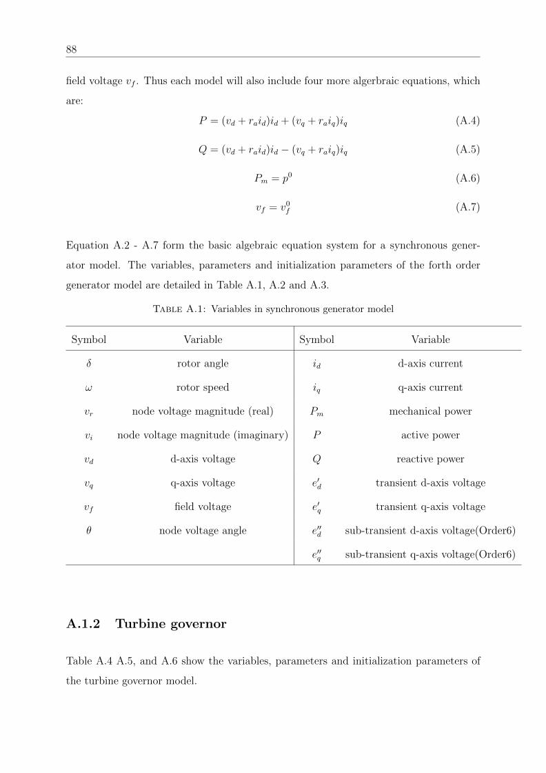
88
field voltage vf . Thus each model will also include four more algerbraic equations, which
are:
P = (vd + raid)id + (vq + raiq)iq (A.4)
Q = (vd + raid)id − (vq + raiq)iq (A.5)
Pm = p0 (A.6)
vf = v0f (A.7)
Equation A.2 - A.7 form the basic algebraic equation system for a synchronous gener-
ator model. The variables, parameters and initialization parameters of the forth order
generator model are detailed in Table A.1, A.2 and A.3.
Table A.1: Variables in synchronous generator model
Symbol Variable Symbol Variable
δ rotor angle id d-axis current
ω rotor speed iq q-axis current
vr node voltage magnitude (real) Pm mechanical power
vi node voltage magnitude (imaginary) P active power
vd d-axis voltage Q reactive power
vq q-axis voltage e′d transient d-axis voltage
vf field voltage e′q transient q-axis voltage
θ node voltage angle e′′d sub-transient d-axis voltage(Order6)
e′′q sub-transient q-axis voltage(Order6)
A.1.2 Turbine governor
Table A.4 A.5, and A.6 show the variables, parameters and initialization parameters of
the turbine governor model.

89
Table A.2: Parameter in synchronous generator model
Symbol Parameter Unit
Sn power rating MVA
Vn nominal voltage kV
fn frequency rating Hz
xl leakage reactance p.u.
ra armature resistance p.u.
xd d-axis reactance p.u.
x′d d-axis transient reactance p.u.
x′′d d-axis sub-transient reactance (Order 6) p.u.
T ′d0 d-axis transient time constant s
T ′′d0 d-axis sub-transient time constant (Order 6) s
xq q-axis reactance p.u.
x′q q-axis transient reactance p.u.
x′′q q-axis sub-transient reactance (Order 6) p.u.
T ′q0 q-axis transient time constant s
T ′′q0 q-axis sub-transient time constant (Order 6) s
M = 2H mechanical starting time kWs/kVA
D damping constant -
Kw speed feedback gain gain
KP active power feedback gain gain
S(1.0) first saturation ratio at node -
S(1.2) second saturation ratio at node -
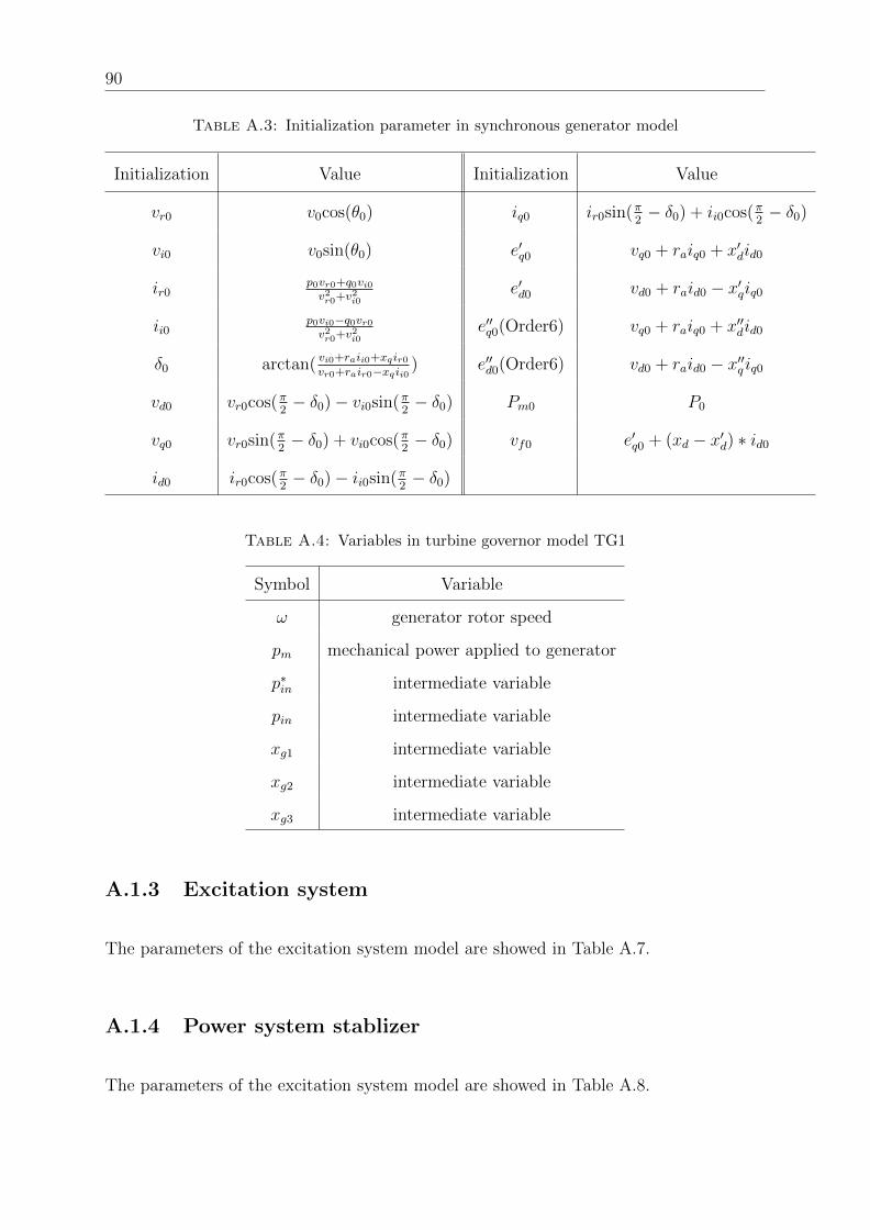
90
Table A.3: Initialization parameter in synchronous generator model
Initialization Value Initialization Value
vr0 v0cos(θ0) iq0 ir0sin(π2− δ0) + ii0cos(π
2− δ0)
vi0 v0sin(θ0) e′q0 vq0 + raiq0 + x′did0
ir0p0vr0+q0vi0v2r0+v
2i0
e′d0 vd0 + raid0 − x′qiq0
ii0p0vi0−q0vr0v2r0+v
2i0
e′′q0(Order6) vq0 + raiq0 + x′′did0
δ0 arctan( vi0+raii0+xqir0vr0+rair0−xqii0 ) e′′d0(Order6) vd0 + raid0 − x′′q iq0
vd0 vr0cos(π2− δ0)− vi0sin(π
2− δ0) Pm0 P0
vq0 vr0sin(π2− δ0) + vi0cos(π
2− δ0) vf0 e′q0 + (xd − x′d) ∗ id0
id0 ir0cos(π2− δ0)− ii0sin(π
2− δ0)
Table A.4: Variables in turbine governor model TG1
Symbol Variable
ω generator rotor speed
pm mechanical power applied to generator
p∗in intermediate variable
pin intermediate variable
xg1 intermediate variable
xg2 intermediate variable
xg3 intermediate variable
A.1.3 Excitation system
The parameters of the excitation system model are showed in Table A.7.
A.1.4 Power system stablizer
The parameters of the excitation system model are showed in Table A.8.

91
Table A.5: Parameter in turbine governor model TG1
Symbol Parameter Unit
ωref reference speed p.u.
pref reference active power p.u.
R droop p.u.
pmax maximum turbine output p.u.
pmin minimum turbine output p.u.
Ts governor time constant s
Tc Servo time constant s
T3 transient gain time constant s
T4 power fraction time constant s
T5 reheat time constant s
Table A.6: Initialization parameter in turbine governor model TG1
Initialization Value
ω ω0
pm0 p0
p∗in0 p0
xg10 p0
xg20 (1− T3Tc
)p0
xg30 (1− T4T5
)(xg20 + xg10T3Tc
)
A.1.5 Load tap changer
The parameters of the LTC model are showed in Table A.9.

92
Table A.7: Parameter in excitation system model EXAC1
Symbol Parameter Unit
TR voltage input time constant s
TB AVR lead-lag time constant s
TC AVR lead-lag time constant s
KA AVR gain p.u.
TA AVR time constant s
VRMAX maximum AVR output p.u.
VRMIN Servo time constant p.u.
TE Exciter time constant. s
KF Rate feedback gain p.u.
VREF Reference terminal voltage p.u.
TF Rate feedback time constant s
KC Rectifier load factor p.u.
KD Exciter demagnetizing factor p.u.
KE Exciter field factor p.u.
E1 Exciter saturation point 1 p.u.
E2 Exciter saturation point 2 p.u.
SE1 Saturation at E1 -
SE2 Saturation at E1 -
A.2 Validation results
1. Forth Order generator
The simulation results of Modelica model and reference model for forth order generator
are shown in Figure A.1.
2. Sixth Order generator
The simulation results of Modelica model and reference model for sixth order generator
are shown in Figure A.2.
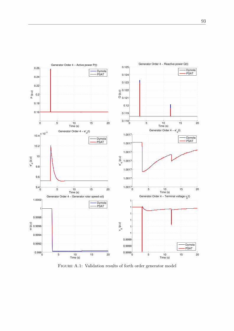
93
0 5 10 15 20
0.16
0.18
0.2
0.22
0.24
0.26
Time (s)
P (
p,u
)
Generator Order 4 − Active power P(t)
Dymola
PSAT
0 5 10 15 200.118
0.119
0.12
0.121
0.122
0.123
0.124
0.125
Time (s)
Q (
p,u
)
Generator Order 4 − Reactive power Q(t)
Dymola
PSAT
0 5 10 15 209.4
9.6
9.8
10
10.2
10.4x 10
−3
Time (s)
e′ d
(p,u
)
Generator Order 4 − e′d(t)
Dymola
PSAT
0 5 10 15 201.0017
1.0017
1.0017
1.0017
1.0017
1.0017
1.0017
Time (s)
e′ q
(p
,u)
Generator Order 4 − e′q(t)
Dymola
PSAT
0 5 10 15 200.999
0.9992
0.9994
0.9996
0.9998
1
1.0002
Time (s)
ω (
p,u
)
Generator Order 4 − Generator rotor speed ω(t)
Dymola
PSAT
0 5 10 15 200.9999
0.9999
0.9999
1
1
1
1
1
1
Time (s)
vg (
p,u
)
Generator Order 4 − Terminal voltage vg(t)
Dymola
PSAT
Figure A.1: Validation results of forth order generator model

94
0 5 10 15 20
0.16
0.18
0.2
0.22
0.24
0.26
Time (s)
P (
p,u
)Generator Order 6 − Active power P(t)
Dymola
PSAT
0 5 10 15 200.118
0.119
0.12
0.121
0.122
0.123
0.124
0.125
Time (s)
Q (
p,u
)
Generator Order 6 − Reactive power Q(t)
Dymola
PSAT
0 5 10 15 209.2
9.4
9.6
9.8
10
10.2
10.4x 10
−3
Time (s)
e′ d
(p
,u)
Generator Order 6 − e′d(t)
Dymola
PSAT
0 5 10 15 201.0017
1.0017
1.0017
1.0017
1.0017
1.0017
1.0017
Time (s)
e′ q
(p
,u)
Generator Order 6 − e′q(t)
Dymola
PSAT
0 5 10 15 200.011
0.0115
0.012
0.0125
0.013
Time (s)
e′′
d (
p,u
)
Generator Order 6 − e′′d(t)
Dymola
PSAT
0 5 10 15 20
1.0013
1.0013
1.0014
1.0014
1.0014
1.0014
Time (s)
e′′
q (
p,u
)
Generator Order 6 − e′′q(t)
Dymola
PSAT
0 5 10 15 200.999
0.9992
0.9994
0.9996
0.9998
1
1.0002
Time (s)
ω (
p,u
)
Generator Order 6 − Generator rotor speed ω(t)
Dymola
PSAT
0 5 10 15 201.0001
1.0002
1.0002
1.0002
1.0002
1.0002
Time (s)
vg (
p,u
)
Generator Order 6 − Terminal voltage vg(t)
Dymola
PSAT
Figure A.2: Validation results of sixth order generator model
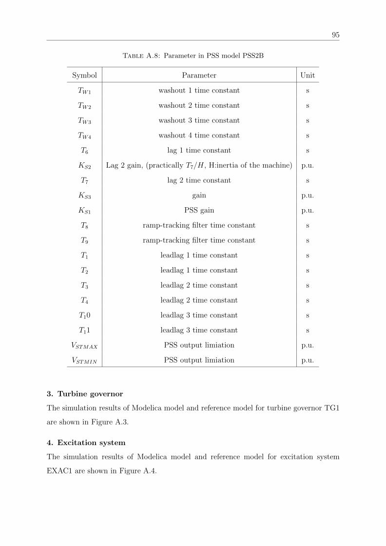
95
Table A.8: Parameter in PSS model PSS2B
Symbol Parameter Unit
TW1 washout 1 time constant s
TW2 washout 2 time constant s
TW3 washout 3 time constant s
TW4 washout 4 time constant s
T6 lag 1 time constant s
KS2 Lag 2 gain, (practically T7/H, H:inertia of the machine) p.u.
T7 lag 2 time constant s
KS3 gain p.u.
KS1 PSS gain p.u.
T8 ramp-tracking filter time constant s
T9 ramp-tracking filter time constant s
T1 leadlag 1 time constant s
T2 leadlag 1 time constant s
T3 leadlag 2 time constant s
T4 leadlag 2 time constant s
T10 leadlag 3 time constant s
T11 leadlag 3 time constant s
VSTMAX PSS output limiation p.u.
VSTMIN PSS output limiation p.u.
3. Turbine governor
The simulation results of Modelica model and reference model for turbine governor TG1
are shown in Figure A.3.
4. Excitation system
The simulation results of Modelica model and reference model for excitation system
EXAC1 are shown in Figure A.4.

96
Table A.9: Parameter in LTC model
Symbol Parameter Unit
Vl0 Initial load voltage p.u.
r0 Initial transformer ratio -
Vmin maximum load voltage p.u.
Vmax minimum load voltage p.u.
nmin minimum transformer ratio -
nmax maximum transformer ratio -
N number of positions -
τ1 first tap change delay s
τ2 subsequent tap change delay s
0 5 10 15 200.15
0.155
0.16
0.165
0.17
0.175
0.18
Time (s)
Pm
(p
.u)
TG1 Test − Mechanical power Pm(t)
Dymola
PSAT
0 5 10 15 200.999
0.9995
1
1.0005
Time (s)
ω (
p.u
)
TG1 Test − Speed ω (t)
Dymola
PSAT
Figure A.3: Validation results of turbine governor model
5. PSS
The simulation results of Modelica model and reference model for PSS are shown in
Figure A.5.
6. LTC
The simulation results of Modelica model and reference model for PSS are shown in
Figure A.6.
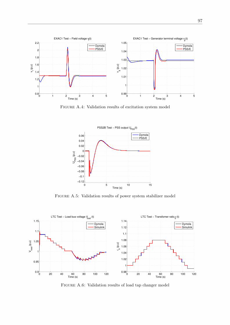
97
0 1 2 3 4 50.8
1
1.2
1.4
1.6
1.8
2
2.2
Time (s)
vf (
p,u
)
EXAC1 Test − Field voltage vf(t)
Dymola
PSS/E
0 1 2 3 4 50.99
1
1.01
1.02
1.03
1.04
1.05
Time (s)
vg (
p,u
)
EXAC1 Test − Generator terminal voltage vg(t)
Dymola
PSS/E
Figure A.4: Validation results of excitation system model
0 5 10 15
−0.12
−0.1
−0.08
−0.06
−0.04
−0.02
0
0.02
0.04
0.06
Time (s)
UP
SS (
p,u
)
PSS2B Test − PSS output UPSS
(t)
Dymola
PSS/E
Figure A.5: Validation results of power system stabilizer model
0 20 40 60 80 100 1200.9
0.95
1
1.05
1.1
1.15
Time (s)
Vlo
ad (
p,u
)
LTC Test − Load bus voltage Vload
(t)
Dymola
Simulink
0 20 40 60 80 100 1200.98
1
1.02
1.04
1.06
1.08
1.1
1.12
1.14
Time (s)
r b (
p,u
)
LTC Test − Transfomer ratio rb (t)
Dymola
Simulink
Figure A.6: Validation results of load tap changer model

98
A.3 Models validated vs Simulink
1. Excitation system with OEL and PSS
The excitation system shown in figure 4.11 consists of three components: Exciter (AVR),
OEL and PSS.
• OEL: OEL model has two input signals: the generator filed current ifd and the
generator terminal voltage. OEL has inverse time characteristics, i.e. the higher the
field current, the faster the limitation takes place. In normal operating conditions,
ifd < ilimfd , the minimum gate passes on the V 0 − V to the AVR; if ifd > ilimfd , the
minimum gate passes on the OEL output signal to the AVR.
• PSS: PSS uses the rotor speed ω as input. Each PSS includes a washout filter and
two identical lead filters in cascade.
• AVR: The AVR is represented by a first-order system, and includes a transient gain
reduction.
The validation results are shown in figure A.7.
0 10 20 30 40 501
1.05
1.1
1.15
1.2
1.25
1.3
1.35
1.4
1.45
Time (s)
ω (
p,u
)
EXC Test − Generator speed ω (t)
Dymola
Simulink
0 10 20 30 40 500.4
0.6
0.8
1
1.2
1.4
Time (s)
vf (
p,u
)
EXC Test − Field voltage vf (t)
Dymola
Simulink
0 10 20 30 40 500.98
0.985
0.99
0.995
1
1.005
1.01
1.015
Time (s)
vg (
p,u
)
EXC Test − Generator terminal voltage vg (t)
Dymola
Simulink
Figure A.7: Validation results of excitation system model
2. Turbine and speed governor
The governor model shown in figure 4.12 has two input signals: the generator active
power P and the generator speed ω. The output of the block is the gate opening z that
applied to the turbine. The turbine model has two input signals: the gate opening z
and the generator speed ω. The output of the block is the torque Tm that applied to the
generator. The validation results are shown in figure A.8.

99
0 20 40 60 801
1.005
1.01
1.015
1.02
1.025
1.03
1.035
Time (s)
ω (
p,u
)
Gov Test − Generator speed ω (t)
Dymola
Simulink
0 20 40 60 800.04
0.06
0.08
0.1
0.12
0.14
0.16
0.18
Time (s)
Pm
(p
,u)
Gov Test − Mechanical power Pm
(t)
Dymola
Simulink
Figure A.8: Validation results of gorvernor and turbine model
A.4 Models validated vs PSAT
1. AVR Type II
The AVR model shown in figure A.9 has two input signals: the terminal voltage vg and
the reference voltage vref . The output of the model is the field voltage vf applied to the
generator. The validation results are shown in figure A.10.
Figure A.9: AVR Type II model [2]
0 5 10 15 200.9
1
1.1
1.2
1.3
1.4
1.5
Time (s)
vf
(p,u
)
EXC2 Test − Field voltage vf(t)
Dymola
PSAT
0 5 10 15 200.8
0.85
0.9
0.95
1
1.05
Time (s)
vg
(p
,u)
EXC2 Test − Generator terminal voltage vg(t)
Dymola
PSAT
Figure A.10: Validation results of AVR Type II model
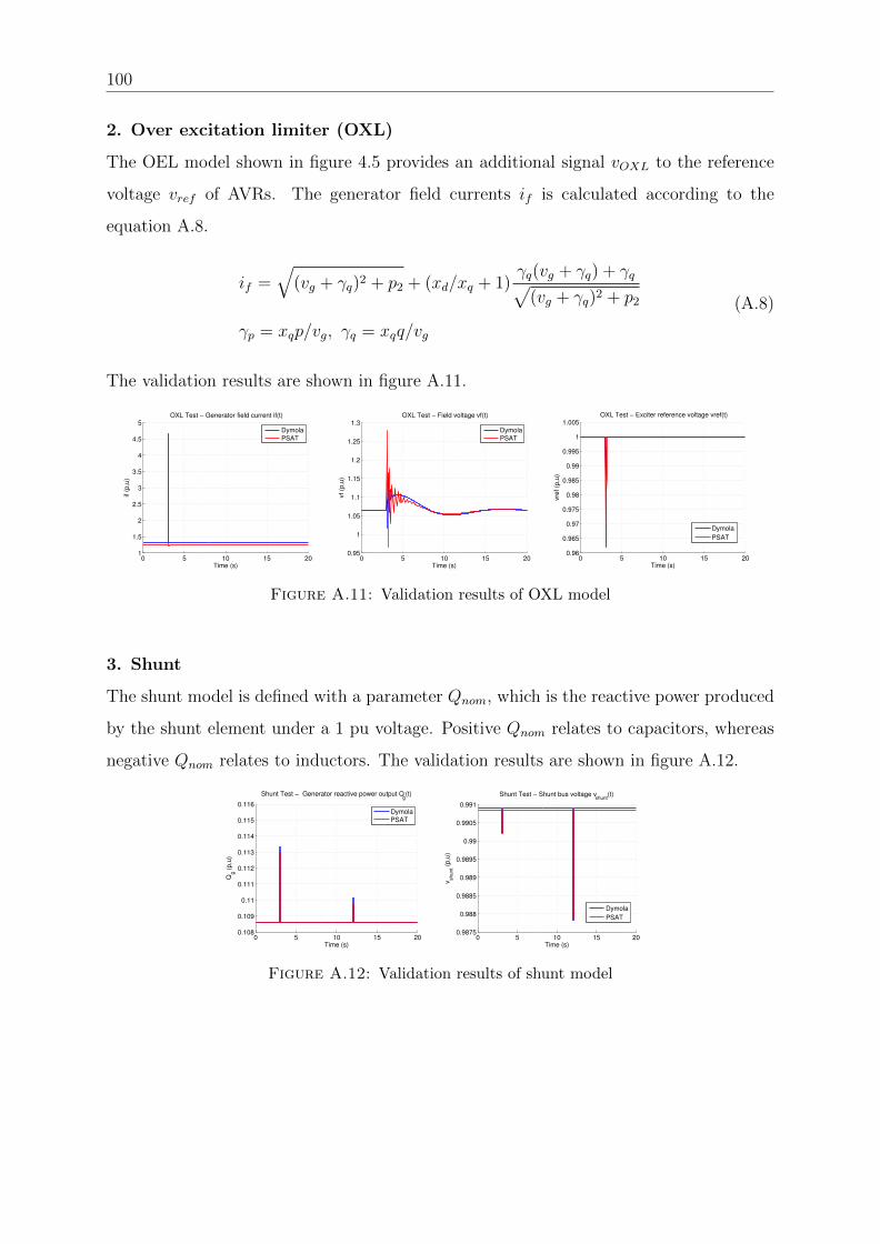
100
2. Over excitation limiter (OXL)
The OEL model shown in figure 4.5 provides an additional signal vOXL to the reference
voltage vref of AVRs. The generator field currents if is calculated according to the
equation A.8.
if =√
(vg + γq)2 + p2 + (xd/xq + 1)γq(vg + γq) + γq√
(vg + γq)2 + p2
γp = xqp/vg, γq = xqq/vg
(A.8)
The validation results are shown in figure A.11.
0 5 10 15 201
1.5
2
2.5
3
3.5
4
4.5
5
Time (s)
if (
p,u
)
OXL Test − Generator field current if(t)
Dymola
PSAT
0 5 10 15 200.95
1
1.05
1.1
1.15
1.2
1.25
1.3
Time (s)
vf
(p,u
)
OXL Test − Field voltage vf(t)
Dymola
PSAT
0 5 10 15 200.96
0.965
0.97
0.975
0.98
0.985
0.99
0.995
1
1.005
Time (s)
vre
f (p
,u)
OXL Test − Exciter reference voltage vref(t)
Dymola
PSAT
Figure A.11: Validation results of OXL model
3. Shunt
The shunt model is defined with a parameter Qnom, which is the reactive power produced
by the shunt element under a 1 pu voltage. Positive Qnom relates to capacitors, whereas
negative Qnom relates to inductors. The validation results are shown in figure A.12.
0 5 10 15 200.108
0.109
0.11
0.111
0.112
0.113
0.114
0.115
0.116
Time (s)
Qg (
p,u
)
Shunt Test − Generator reactive power output Qg(t)
Dymola
PSAT
0 5 10 15 200.9875
0.988
0.9885
0.989
0.9895
0.99
0.9905
0.991
Time (s)
vshunt (
p,u
)
Shunt Test − Shunt bus voltage vshunt
(t)
Dymola
PSAT
Figure A.12: Validation results of shunt model

101
A.5 Models validated vs PSS/E
1. Speed governor IEEEG1
The governor model shown in figure A.13 is designed for thermal turbines and governors.
The input of the model is ∆ω, the variation of generator speed. Outputs of the model
are mechanical power PMECHHP and PMECHLP to be connected to the generator. The
validation results are shown in figure A.14.
Figure A.13: Speed governor IEEEG1 model [3]
0 5 10 150.994
0.995
0.996
0.997
0.998
0.999
1
1.001
1.002
1.003
Time (s)
ω (
p,u
)
IEEEG1 Test − Speed ω(t)
Dymola
PSS/E
0 5 10 15
0.04
0.045
0.05
0.055
0.06
0.065
Time (s)
Pm
(p,u
)
IEEEG1 Test − Mechanical power Pm
(t)
Dymola
PSS/E
Figure A.14: Validation results of shunt model


Appendix B
Experiences in modelling and
simulation of large-scale power
systems
This appendix includes the experiences in the modelling, simulation and validation of
large-scale power systems in the project: KTH Nordic 32 system and IEEE Nordic 32
system. In Section B.1 the critical steps are presented, and in Section B.2 the solutions
to some common problems in the process are provided.
B.1 Critical Steps
B.1.1 Preparation
1. Before the implementation of system models, a few principles need to be followed.
The principles are detailed in Chapter 4.2. Among the principles, the most im-
portant one are: “Make appropriate simplification to the system model”.
The first knowledge one needs to know before the modelling of a power system is
that a model cannot represent every aspect of a real system. The engineer needs
103
104
to decide which aspect is more important to represent according to the objective of
the study, and make simplification to the models.
In this project, the types of critical models (generators, generator controllers, trans-
formers, etc.) are already decided, thus there is no space for simplification.
2. After the simplification process, the component models used in the system model
can be selected and prepared. An important task in this step is to make sure that all
models are validated. One can use a small test system (for example: a system with
1-2 generator, 3-4 buses, 1-2 loads and 1-2 faults) to test if the component models
are validated. “Make sure every component model is validated before the
modelling large-scale system” is very important, since if an incorrect model is
included in a large system model, it will be very difficult to figure out which model
is the problem when the system model is giving incorrect responses.
After all component models are prepared, create a new package and include all
component models in it. This step will solve the problem of incorrect path of
models in the modelling process.
3. Another important principle is “Use power flow solution to initialize the
system model”. Other than the component models, another important prepara-
tion is the power flow solution data. The needed data include:
• Generator buses operating point data: Generated active power Pg, generated
reactive power Qg, initial voltage magnitude vg, initial voltage phase angle θg.
• Transmission and distribution buses operating point data: Initial voltage mag-
nitude vb, initial voltage phase angle θb.
B.1.2 Modelling
1. Implement the model of power plants. Each power plant includes one or more
generators and a number of controllers (AVR, governor, turbine, PSS, etc). Other
than connecting all these component models to the system, it is better to integrate
them in one single model first, and then connect it to the system. An example of
the power plant model is shown in Figure 4.1.

105
2. Divide the system into a few parts, and develop independent models for each part.
For instance, in the Nordic 32 system, the system is divided into four parts according
to graphical area. It will make the modelling and simulation process easier to
implement the system parts one by one.
3. Fill in the parameters (component parameters and initial parameters) into the mod-
els. This is the most important step in the modelling process. Even a small error
in the parameters will cause problem in the simulation. It is better to fill in the
parameters in the text view of the system model to avoid omitting any models.
4. Check and compile the model. If the components are correctly connected and all
parameters are correctly filled in, there should not be any errors in this step. If
there are errors, check the connection of component models, and the parameters of
the models.
B.1.3 Simulation and validation
1. Simulate the models for each part (without faults). In this step, the external sys-
tem can be replaced by one or more large loads, depending on how the system is
connected. The simulation results will keep constant in the steady state values.
Since the model includes less component models than the complete system model,
it will be easier to find the reason of problem when the simulation cannot be run
correctly.
2. If all parts can be simulated, it is time to connect all parts together to form the
complete system. Simulate the system model (without faults), and the simulation
results should also be constant, same as the steady state values.
3. Apply faults to the system, and simulate the model again. Revise the model ac-
cording to the comparison of simulation results in reference software and Dymola.
Solutions for possible problems in above two steps can be found in Section B.2.

106
B.2 Solutions to possible problems
1. Q: Fail to check the system model.
A: If the model is failed to be checked, there exist three possible reasons:
• The path of component models are not correct.
• The parameters of component models are not completely filled in.
• The models are not correcrly connected.
2. Q: When trying to simulate one part of the system model, simulation cannot start.
A: In this case, the error information provided by Dymola may be: “Fail to start
the model (simulation)”. In most cases, initialization is the main problem.
Generally, there may be two reasons:
• There exist some variables divided by zero. Before the simulation begins,
Dymola will calculate the initial values for all variables based on the provided
initialization data, thus there may be situations in which the initial values for
some variables are calculated to be zero.
In this case, check the detailed error information provided by Dymola, find the
variables divided by zero, and revise the corresponding model.
• Initialization values conflict. This is a problem happens very frequently. When
initialization information is provided for each model in a interconnected sys-
tem, there may be situation in which initial values for a same variable (obtained
in different models) conflict with each other.
In this case, the key is to find the models in conflict. One solution is to replace
one kind of component model (e.g. load model) by another type of model.
For instance, replace the constant current load models by constant impedance
models. Next, run the simulation again, if the model can be initialized, then
trying to find another method to initialize the constant current load model
may solve the problem.
3. Q: When simulate one part of the system model without faults, cannot obtain
constant simulation results.

107
A: If the simulation can start, but there are oscillations in the results even from the
very beginning of the simulation, it shows that there still exists problem with the
initialization, but not as severe as the case in Q2. The solution is similar: change
the type of one particular model to see if the situation is improved.
4. Q: The simulation results of each small part of system model look fine, but when
connect them together to form the complete system, the simulation cannot start.
A: The reason is similar: initialization conflict. Firstly start from connecting the
smaller parts, try to find the models in conflict, and revise the initialization method
in the model.
5. Q: The simulation results of complete system model look fine without fault, but
when the fault is applied, the simulation cannot start.
A: Firstly, try different types of fault, and different positions to apply the fault. If
it turns out that other types of fault can be simulated, or the fault can be simulated
in other positions , then revise the fault model or model the fault in another way
may solve the problem. If it turns out that no type of fault can be simulated, then
change the fault to be less severe to see if the situation can be improved.
6. Q: The system model can be simulated, but cannot match the reference well.
A: Other than try to find problem in the models, change the simulation parameters
may also help to improve the situation. The integration algorithm, integration
step and output interval length can be changed. One should not rely on just one
integration method, but two or three other integration methods can be applied to
find a better result.
Other than the problems listed above, there may be a large number of possible problems
in the modelling and simulation process. However, the solution can be general. When
the reasons of problems are hard to found, the most practical method is: to change the
models in every possible aspect, from the initialization data to the model description.
Changes of models will bring variations in the simulation results, and these variations
will show the right direction for the correction.

Bibliography
[1] Eric Allen, DN Kosterev, and Pouyan Pourbeik. Validation of power system models.
In Power and Energy Society General Meeting, 2010 IEEE, pages 1–7. IEEE, 2010.
[2] Federico Milano. Power system analysis toolbox documentation for psat version
2.1.8, 2013.
[3] PTI Siemens. Pss R© e 33.2 program operation manual, 2012.
[4] Yuwa Chompoobutrgool and Luigi Vanfretti. Linear analysis of the kth-nordic32
system. 2011.
[5] IEEE PES PSDP Commitee. Ieee task force report: Test systems for voltage stability
and security assessment. 2013.
[6] J-P Barret, Pierre Bornard, Bruno Meyer, and Bruno Meyer. Power system simula-
tion. Springer, 1997.
[7] Petros Aristidou. Power system simulation challenges. 8th IntelliCIS Workshop,
04-03-2013 to 08-03-2013 .
[8] Luigi Vanfretti, Tetiana Bogodorova, and Maxime Baudette. A modelica power
system component library for model validation and parameter identification.
[9] Federico Milano. Power system modelling and scripting. Springer, 2010.
[10] Dennis Woodford. Introduction to pscad v3. Manitoba HVDC Research Centre Inc,
pages 400–1619, 2001.
[11] DIgSILENT Power Factory Manual and DIgSILENT PowerFactory. Version 14.0.
DIgSILENT GmbH, Gomaringen, Germany, 2009.
109

Bibliography
[12] Dimitris Peppas. Development and analysis of nordic32 power system model in
powerfactory. 2008.
[13] Dmitry N Kosterev, Carson W Taylor, and William A Mittelstadt. Model validation
for the august 10, 1996 wscc system outage. Power Systems, IEEE Transactions on,
14(3):967–979, 1999.
[14] Francisco Gomez, Luigi Vanfretti, and Svein Harald Olsen. A modelica-based exe-
cution and simulation engine for automation power system model validation.
[15] Rogersten Robert, Vanfretti Luigi, and Li Wei. Towards consistent model exchange
and simulation of vsc-hvdc controls for emt studies through c-code integration.
[16] Angela S Chieh, Patrick Panciatici, and Jerome Picard. Power system modeling in
modelica for time-domain simulation. In PowerTech, 2011 IEEE Trondheim, pages
1–8. IEEE, 2011.
[17] Tetiana Bogodorova, Marc Sabate, Gladys Leon, Luigi Vanfretti, Milenko Halat,
Jean-Baptiste Heyberger, and Patrick Panciatici. A modelica power system library
for phasor time-domain simulation. In Innovative Smart Grid Technologies Europe
(ISGT EUROPE), 2013 4th IEEE/PES, pages 1–5. IEEE, 2013.
[18] Power System Library SPOT. [online]. URL http://www.modelica.org/
libraries/spot.
[19] ObjectStab Free library for power system voltages ad transient simulation. [online].
URL http://www.modelica.org/libraries/ObjectStab.
[20] iTesla: Innovative Tools for Electrical System Security within Large Areas. [online].
URL http://www.itesla-project.eu.
[21] Modelica Association. Modelica Language Specification, Version 3.3. 2012-05-09.
[22] Peter Fritzson. Principles of object-oriented modeling and simulation with Modelica
2.1. John Wiley & Sons, 2010.
Bibliography 111
[23] Borut Zupancic and Anton Sodja. Advanced multi-domain modelling: advantages
and dangers. In Computer Modelling and Simulation (UKSim), 2011 UkSim 13th
International Conference on, pages 260–265. IEEE, 2011.
[24] Peter Fritzson and Peter Bunus. Modelica-a general object-oriented language for
continuous and discrete-event system modeling and simulation. In Simulation Sym-
posium, 2002. Proceedings. 35th Annual, pages 365–380. IEEE, 2002.
[25] Sven Erik Mattsson, Hilding Elmqvist, Martin Otter, and Hans Olsson. Initialization
of hy-brid differential-algebraic equations in modelica 2.0. In 2nd Inter. Modelica
Conference 2002, pages 9–15, 2002.
[26] AB Dynasym. Dymola dynamic modeling laboratory user’s manual, 2006.
[27] Joan Russinol Mussons. Modelica-driven power system modelling, parameter iden-
tification and physically-based model aggregation. Master’s thesis, KTH, School of
Electrical Engineering, 2013.
[28] DC Lee, DH Baker, KC Bess, et al. Ieee recommended practice for excitation system
models for power system stability studies. Energy development and power generation
committee of power engineering society, 1992.
[29] M. Stubbe (convener). Long-term dynamics - phase ii. Report of CIGRE Task Force,
38.02.08, Jan.1995.
[30] Thierry Van Cutsem and Costas Vournas. Voltage stability of electric power systems,
volume 441. Springer, 1998.
[31] Carson W Taylor. Power system voltage stability. McGraw-Hill, 1994.
[32] Prabha Kundur, Neal J Balu, and Mark G Lauby. Power system stability and control,
volume 7. McGraw-hill New York, 1994.
[33] Lei Wang, Meir Klein, Solomon Yirga, and Prabha Kundur. Dynamic reduction of
large power systems for stability studies. IEEE Transactions on Power Systems, 12
(2):889–895, 1997.
Bibliography
[34] M Larbi Ourari, L-A Dessaint, and Van-Que Do. Dynamic equivalent modeling of
large power systems using structure preservation technique. Power Systems, IEEE
Transactions on, 21(3):1284–1295, 2006.
[35] Thierry Van Cutsem. Description, modelling and simulation results of a test system
for voltage stability analysis. Technical Report Version 1, IEEEWorking Group on
Test Systems for Voltage stability analysis, July.2010.
[36] FP De Mello, PJ Nolan, TF Laskowski, and JM Undrill. Coordinated application
of stabilizers in multimachine power systems. Power Apparatus and Systems, IEEE
Transactions on, (3):892–901, 1980.
[37] Lennart Ljung. System identification. Springer, 1998.
[38] Luigi Vanfretti, Tetiana Bogodorova, and Maxime Baudette. Power system model
identification exploiting the modelica language and fmi technologies. In Intelligent
Energy and Power Systems (IEPS), 2014 IEEE International Conference on, pages
127–132. IEEE, 2014.
[39] Xiuqin Deng. System identification based on particle swarm optimization algorithm.
In Computational Intelligence and Security, 2009. CIS’09. International Conference
on, volume 1, pages 259–263. IEEE, 2009.
[40] Shi-qiang Hu and Zhong-liang Jing. Overview of particle filter algorithm. Control
and Decision, 20(4):361, 2005.
[41] Torsten Blochwitz, M Otter, M Arnold, C Bausch, C Clauß, H Elmqvist, A Jung-
hanns, J Mauss, M Monteiro, T Neidhold, et al. The functional mockup interface
for tool independent exchange of simulation models. In 8th International Modelica
Conference, Dresden, pages 20–22, 2011.
Top Related