


Languages
Pages
Legal


Modeling and Computational Issues
in the Development of Batch Processes
by
Russell John Allgor
Submitted to the Department of Chemical Engineering
in partial ful�llment of the requirements for the degree of
Doctor of Philosophy in Chemical Engineering
at the
MASSACHUSETTS INSTITUTE OF TECHNOLOGY
June ����
c� Massachusetts Institute of Technology ����� All rights reserved�
Author � � � � � � � � � � � � � � � � � � � � � � � � � � � � � � � � � � � � � � � � � � � � � � � � � � � � � � � � � � � � �
Department of Chemical Engineering
June ��� ����
Certi�ed by � � � � � � � � � � � � � � � � � � � � � � � � � � � � � � � � � � � � � � � � � � � � � � � � � � � � � � � � �
Paul I� Barton
Assistant Professor
Thesis Supervisor
Certi�ed by � � � � � � � � � � � � � � � � � � � � � � � � � � � � � � � � � � � � � � � � � � � � � � � � � � � � � � � � �
Lawrence B� Evans
Adjunct Professor
Thesis Supervisor
Accepted by � � � � � � � � � � � � � � � � � � � � � � � � � � � � � � � � � � � � � � � � � � � � � � � � � � � � � � � �
Robert Cohen
St� Laurent Professor of Chemical Engineering
Chairman� Committee on Graduate Students

�

Modeling and Computational Issues
in the Development of Batch Processes
by
Russell John Allgor
Submitted to the Department of Chemical Engineeringon June ��� ����� in partial ful�llment of the
requirements for the degree ofDoctor of Philosophy in Chemical Engineering
Abstract
The rapid development of an e�cient process to manufacture a new or modi�edproduct within an existing batch manufacturing facility is critical to the success ofmany specialty chemical and synthetic pharmaceutical companies This thesis employs process modeling technology as the basis for an integrated batch process development methodology that complements and enhances laboratory and pilot scaleexperimentation Examples demonstrate that signi�cant bene�ts can be realized forthese industries
To develop optimal batch processes using detailed mathematical models� the continuous decisions de�ning the operating policies of the processing tasks and the discrete decisions de�ning the process structure and allocation of plant resources mustbe made simultaneously The �rst rigorous decomposition algorithm that simultaneously considers both types of decisions is derived� the algorithm also extends togeneral mixed time invariant integer dynamic optimization problems This decomposition algorithm requires subproblems that yield rigorous upper and lower bounds onthe objective� and robust numerical techniques to solve each subproblem Screeningmodels are derived to provide rigorous lower bounds on the manufacturing cost� upperbounds on the cost are provided by the solution of a dynamic optimization problemThe robustness� accuracy� and e�ciency of the numerical solution algorithms for thesimulation and optimization of detailed discrete�continuous dynamic models is alsoimproved� allowing the solution of the dynamic optimization subproblem to be performed more reliably
Screening models exploit domain speci�c knowledge to obtain rigorous lower boundson the manufacturing cost The lower bounding property of the screening models isproven for networks of reaction and distillation tasks and demonstrated on severalcase studies that illustrate the ability of the screening models to handle aspects ofprocess synthesis The design targets provided by the solution of these models facilitate rapid decision making during the early stages of process development� enhancethe application of other design methodologies� and facilitate the formulation and solution of the dynamic optimization subproblems required within the decomposition

algorithmSophisticated equation based modeling environments provide modeling exibility
by decoupling the solution procedures from the model de�nition but� at the same time�place severe expectations on the numerical integration techniques The application ofthese environments to the simulation and optimization of batch reaction and distillation tasks uncovers several previously unreported numerical problems This thesisproves that the observed numerical di�culties are caused by an illconditioned corrector iteration matrix� demonstrates that the accuracy of DAE integration codes islimited by the condition number of the corrector iteration matrix� and explains howthe integration code�s error control strategy can permit the generation of �spikes�Automated scaling techniques are developed and implemented to permit the e�cientsolution of poorly scaled problems and to mitigate the e�ects of illconditioned models� it is proven that this scaling comes very close to the optimal scaling for the sparseunstructured matrices with which we are concerned In addition� a novel strategy isdeveloped to start DAE integration codes e�ciently at the frequent discontinuitiesexperienced in such simulations and optimizations
The advantages of this integrated design methodology are demonstrated through aseries of realistic examples exhibiting the complexity of typical industrial applications
Thesis Supervisor� Paul I BartonTitle� Assistant Professor
Thesis Supervisor� Lawrence B EvansTitle� Adjunct Professor

Dedicated to my family for their love�
encouragement� and support�
�Given the pace of technology� I propose we leave math to the machines
and go play outside�
� Calvin� Calvin and Hobbes by Bill Waterson ������


Acknowledgments
I would like to thank Professor Paul Barton for providing guidance and encouragementduring the course of my thesis research I have learned a lot from the discussions wehave had over the years� I truly appreciate the attention you have given my thesisduring the past few months You have been a good advisor and a true friend I wouldalso like to thank Professor Larry Evans for the inspiration driving this research andfor convincing me to come to MIT
I would like to thank the members of my research group and friends for providingme with the opportunity to discuss ideas and broaden my knowledge through fruitfuldiscussions Howard� John� and Santos have taken time to discuss the numericalaspects of my research� allowing me to iron out the details of this portion of myresearch Wade and John have allowed me to spend more time on my research bytaking over the management of the computer systems and ABACUSS Thanks toBill for �xing bugs that I have run into in a timely fashion Taeshin�s generositywith his afternoon snacks has kept me from going hungry over the past few months�and Christophe kept me up to date with the sports news from Europe Thanks toMingjuan and Kamel for helping me with portions of my research� and to Berit formaking sure that I have had a research group through all these years at MIT
I would like to thank Elaine for organizing the recruiting in the departmentShe went out of her way to help me out after my surgery and provided me withopportunities that may have otherwise been wasted
I really appreciate all the support my friends have given me over the past fewyears Without their support I would not have been able to get this far The soccerteam at MIT has given me some great friends and really helped me to enjoy the timeI have spent here Special thanks to Walter� Josh� and Ste�en who have kept theteam organized and made the game a lot of fun I�m also glad that Alex decided togo to HBS for school It was great to have a good friend in the area who was notassociated with MIT
Most of all� I would like to thank my family The past year has been extremelydi�cult for me� and the love and support you have given me has helped me getthrough the thesis� recover from back surgery� and deal with everything else that hashappened Mom and Dad� you have come to my aid when I needed your help Alison�your visits to Boston were a great help I know I can always count on your support
In conclusion� I would like to thank the US Department of Energy for �nancialsupport

�

Contents
� Introduction ��
�� Batch Process Manufacturing ���� Batch Process Development ���� Design Methods for Batch Process Development ���� Screening Models for Batch Process Development ���� Rigorous Decomposition Algorithm ���� Numerical Issues in the Detailed Simulation of Batch Processes ���� Outline of Thesis ��
� Batch Process Development ��
�� Previous Research ����� Design with Fixed Recipes ����� Design with Recipe Modi�cations ����� Coupling the Structure and Performance Subproblems ��
�� Applying Screening Models to Process Development ���� Scope of Development Problems Considered ���� Decomposition Algorithm for Batch Process Development ���� Summary ��
� Screening Models for Batch Process Development ��
�� Deriving Screening Models for Reaction�Distillation Networks ����� Process Abstraction ����� Batch Distillation Composition Bounds ����� Reactor Targeting Model ��
�� Time Averaged Material Balances ���� Bounding Distillation Processing Time and Utility Requirements ��
��� Distillation Processing Time Bounds ����� Bounding the Distillation Utility Requirements ����� De�nition of Bottoms Cuts ���
�� Equipment Allocation ����� Process Performance and Production Cost ����� Formulating the model to be solved ����� Conclusions ����� Notation ���
��� Indexed Sets ���
�

��� Integer Variables ������ Binary Variables ������ Exact linearizations of bilinear products of binary variables ������ Continuous Variables ������ Parameters ���
� Using Screening Models to Identify Favorable Processing Structures���
�� Process Description ����� Design Constraints ����� Reaction targets ���
��� Bounding the selectivity and extent of reaction ������ Convexifying the Extent�Time Boundaries ������ Minimum Extents of Reaction ���
�� Process Superstructure ����� Solutions of the Screening Models ���
��� Solution obtained from the First Superstructure ������ Solution obtained from the Second Superstructure ������ Solution Comparison ���
�� Computational Considerations ������ Size of the Models solved ������ Scaling of the Linear Programs ������ Solution Procedure ������ Linearization of Bilinear Terms ������ In uencing the Branch and Bound Algorithm ������ Tailored Solution Procedures ������ Representation of Batch Distillation Boundaries ���
�� Summary ����� Notation ���
��� Indexed Sets ������ Binary Variables ������ Variables ������ Parameters ���
� Siloxane Monomer Case Study ���
�� Laboratory Scale Process ������ First Reaction Task ������ Second Reaction Task ������ Third Reaction Task ������ Design Constraints ���
�� Case Study I� Comparison of minimum cost versus minimum waste ������ Solution ���
�� Case Study II� Including Reaction Targets ������ First Reaction Task ������ Solutions to Case Study II ������ Case III� Disposing of Recycle Streams ���
��

�� Conclusions ���
� Numerical Issues in the Simulation and Optimization of Hybrid Dy�
namic Systems ��
�� Accuracy of Solution Procedures ������ Backward Error and Conditioning ���
�� E�ciency of Integration Codes ����� Mathematical Background ���
��� BDF Integration Codes ������ Dynamic Optimization ������ Rounding Error Analysis ������ Scaling of Linear Systems ������ Row Equilibration ������ Properties of Newton�s Method ���
�� Summary ���
� Automatic Scaling of Dierential�Algebraic Systems ���
��� Modeling Flexibility Derived from the Automatic Scaling ofDAE Models ���
�� Demonstration of Problem ����� Explanation of the Phenomenon ���
��� Generation of a �spike� ������ Truncation Error Criterion ���
�� Illconditioned Corrector Iterations ����� Sti�ness� Conditioning� and Index ���
��� Sti�ness and Conditioning of ODEs ������ Conditioning of ODE and DAE systems ������ Modeling Decisions Related to the Index ������ The myth of �Near Index� Systems ���
�� Scaling Variables and Equations ������ Scaling the Variables ������ Scaling the Equations ���
�� Automatic Detection of Potential Inaccuracy ����� E�ect of Scaling ����� Conclusions ���
� Initial Step Size Selection for Dierential�Algebraic Systems ���
�� Introduction ����� Initial Step Size Selection ����� Scope ����� Methodology ����� Consistent initial conditions ����� Derivatives of algebraic variables ����� Initial step size ���
��� De�ning the optimal initial step size ���
��

��� Initial step size estimator ������ Initial time step combined with step size selection ���
�� Implementation within DSL��S ����� Computational Performance ������ Conclusions ���
� Mixed�Integer Dynamic Optimization ���
�� Introduction ����� Problem Scope ����� Applying MINLP algorithms ����� Decomposition Approach to MIDO ����� Casting Batch Process Development as a MIDO ���
��� Distillation Column Constraints ������ Reaction Constraints ���
�� Application of the MIDO Decomposition Algorithm ����� Summary ����� Notation ���
��� Indexed Sets ������ Variables ������ Time Invariant Integer Optimization Parameters ������ Control Variables ������ Time Invariant Continuous Optimization Parameters ������ Parameters ���
� Conclusions and Recommendations ���
��� Screening Models for Batch Process Development ������ Numerical Issues in the Simulation and Optimization of Hybrid Dis
crete�Continuous Dynamic Systems ������ Recommendations for Future Research ���
A Matrix and Vector Norm Proofs ���
A� Comments on condition numbers� inf� sup� and rectangular matrices ���
B Solution of an augmented system of linear equations ���
C Time derivatives of the algebraic sensitivity variables ���
D Review of Batch Plant Design Literature ���
D� Multiple Products ���D� Semicontinuous units ���D� Parallel Units ���D� Multipurpose Plants ���D� Varying the Task to Stage Assignment ���D� Discrete Equipment Sizes ���D� Intermediate Storage ���D� Design Under Uncertainty ���
��

D� Solution Methods ���D�� Conclusions ���
Bibliography ���
��

��

List of Figures
�� Sequential design procedure often used for process development ��
�� Ad hoc iteration iteration strategy employed in an evolutionary approach ��
�� Decomposition algorithm for batch process development ��
�� The two nesting strategies for the performance and structure subproblems investigated by Barrera ������ ��
�� Schematic of the information provided to and produced by the screening formulations ��
�� Plant Superstructure for Batch Reactor ��
�� State Task Network for Batch Reaction ��
�� The state task network for dynamic optimization of the process development example from chapter � This corresponds to the screeningmodel solution obtained from the �rst process superstructure ��
�� Superstructure for networks of reaction and separation tasks ��
�� Residue curve map for a ternary system with pure components ������ and �� The �xed point �� represents a maximum boiling binaryazeotrope between �� and �� ��
�� Ternary system with two distillation regions showing the pot composition trajectory for a feed in distillation region I ��
�� Representation of an arbitrary distillation task by combining sharpdistillation cuts and mixers ��
�� Detailed representation of �xed point node e used to derive the purgeconstraints ��
�� Distillation regions projected onto the facet formed by B� W�� and P ���
�� Surface de�ning the upper bound on the extents of reaction given byf��� e��t� ���
�� Process schematic of the solution derived from the superstructure containing only one reaction task Fixed point ows are given in kmols ���
�� Process schematic of the solution derived from the superstructure permitting multiple reaction tasks Fixed point ows are given in kmols ���
�� Process schematic of the solution derived for Case IA Streams labelsdenote the ow of each �xed point in kmols for the campaign ���
��
�� Process schematic of the solution derived from the superstructure containing only one reaction task Streams labels denote the ow of each�xed point in kmols for the campaign ���
�� Process schematic of the solution derived from the superstructure requiring all three reaction tasks Streams labels denote the ow of each�xed point in kmols for the campaign ���
�� Process schematic of the solution derived from the superstructure containing only one reaction task in which the disposal of recycle streamsat the end of the campaign is considered Stream labels indicate the�xed point ows for the campaign given in kmols ���
�� Plot of condenser duty resulting from ABACUSS simulation showingone �spike� in detail ���
�� Flowchart for the predictor corrector implementation of the BDF method����� Implementation of the dynamic optimization algorithm within ABA
CUSS ���
�� �Spikes� in the time pro�le of the condenser duty ����� One of the �spikes� shown in detail ����� A comparison of the predicted and corrected solution as a function of
the step size during the generation of a spike ����� Relationship between the exact Newton update �x� the numerically
calculated Newton update �x� and the convergence tolerance � ����� Values for x� and x� for the index� system and when � � ���� ����� Demonstration of the di�erence between � � �� and the other values of ������ The decay of y onto the high index manifold for di�erent � ����� The solution the index� system found by solving the equivalent index
� system ��������� ����� The unstable solution of the index� system ���
�� Flowchart of the MIDO decomposition algorithm ����� Sequence of subproblem solutions that could be obtained from the
MIDO decomposition algorithm ����� The superstructure for the MIDO formulation of the process develop
ment example from chapter � ����� Decomposition algorithm employed for MINLP problems ����� MIDO decomposition algorithm when a convex MINLP screening model
is employed ���
��

List of Tables
�� Constants for the Arrhenius rate expressions for the �rst order reaction
rates �ri � Cikie�EART � ���
�� Azeotrope compositions for the three azeotropes formed between B�W�� and P ���
�� Product cut sequences for the distillation regions ���
�� Inventory and rental rates for processing equipment ���
�� Material cost� disposal cost� and physical property data for the �xedpoints ���
�� Raw material costs for the design obtained from the �rst superstructure���
�� Waste disposal costs for the design obtained from the �rst superstructure���
�� Utility costs for the design obtained from the �rst superstructure ���
�� Equipment costs for the design obtained from the �rst superstructure ���
��� Comparison of raw material� waste disposal� utility� and equipment forthe design obtained from the �rst superstructure ���
��� Equipment utilization for the design obtained from the �rst superstructure ���
��� Raw material costs for the design obtained from the second superstructure ���
��� Waste disposal costs for the design obtained from the second superstructure ���
��� Utility costs for the design obtained from the second superstructure ���
��� Equipment costs for the design obtained from the second superstructure���
��� Equipment utilization for the design obtained from the second superstructure ���
��� Comparison of raw material� waste disposal� utility� and equipmentcosts obtained for the second superstructure ���
��� Comparison of the manufacturing costs of the solutions obtained fromthe two superstructures examined ���
��� Size and approximate solution times for the screening models solved inchapters � and � on an HP J��� workstation ���
�� Preexponential factors and activation energies de�ning the rate constants �������� for reactions ������� occurring within the �rst reaction task ���
��

�� Feasible product sequences for the �rst case study of the siloxanemonomer process ���
�� Composition of the �xed points that are not pure components ����� Cost and physical property data for the �xed points ����� Inventory and rental rates for processing equipment ����� Utility cost data for the siloxane monomer example ����� Raw material costs for the entire campaign when minimizing total cost
in the �rst case study ����� Waste disposal costs for the entire campaign when minimizing total
cost in the �rst case study ����� Utility costs for the entire campaign when minimizing total cost in the
�rst case study ������ Equipment costs for the entire campaign when minimizing total cost
in the �rst case study ������ Equipment utilization for the design obtained when minimizing total
cost in the �rst case study ������ Comparison of raw material� waste disposal� utility� and equipment costs������ Feasible product sequences for the second case study of the siloxane
monomer process ������ Raw material costs for the entire campaign for the process containing
only one reaction task ������ Utility costs for the distillations for the entire campaign for the process
containing only one reaction task ������ Equipment costs for the entire campaign for the process containing
only one reaction task ������ Equipment utilization for the design obtained from the process con
taining one reaction task ������ Comparison of raw material� waste disposal� utility� and equipment
costs for the process containing only one reaction task ������ Raw material costs for the entire campaign for the process requiring
three reaction tasks ������ Utility costs for the distillations for the entire campaign for the process
requiring three reaction tasks ������ Equipment costs for the entire campaign for the process requiring three
reaction tasks ������ Equipment utilization for the design obtained from the process requir
ing three reaction tasks ������ Comparison of raw material� waste disposal� utility� and equipment
costs for the process containing only one reaction task ������ Raw material costs for the process considering the disposal of recycled
material at the completion of the campaign ������ Waste disposal costs for the process considering the disposal of recycled
material at the completion of the campaign ������ Utility costs for the distillation task in the process considering the
disposal of recycled material at the completion of the campaign ���
��

��� Equipment costs for the process considering the disposal of recycledmaterial at the completion of the campaign ���
��� Equipment utilization for the process considering the disposal of recycled material at the completion of the campaign ���
��� Comparison of raw material� waste disposal� utility� and equipmentcosts for the process considering the disposal of recycled material atthe completion of the campaign ���
�� Value of the local truncation error parameter M in the limits of constant and drastically reduced step sizes ���
�� Numerical statistics for the solution of ��������� at di�erent valuesof � ���
�� Performance of integration code on combined simulation test problemsusing the initial step length heuristics employed by DASSL ���
�� Performance of integration code on combined simulation test problemsusing the optimal initial step length calculation ���
��

��

Chapter �
Introduction
Process modeling technology has changed the way in which continuous�steady state
chemical processes are designed and operated �Evans� ������ yet a similar impact
has not yet been witnessed for the design of batch processes The dynamic nature
of batch processing operations coupled with the combinatorial aspects of equipment
scheduling and resource allocation dictate that the e�ective application of process
modeling to the design of batch processes is a more formidable task
Recent advances in modeling capabilities and optimization techniques for dynamic
processes now permit the application of detailed modeling technology to batch pro
cesses �Barton� ����� However� the bene�ts a�orded by the application of modeling
techniques must outweigh the e�ort and time required to generate the models� and
apply the design methodology Drawing the analogy to continuous processes� we feel
that process modeling techniques can reap the most signi�cant bene�ts when applied
to the design of batch processes by empowering the engineer to exploit interactions
between the processing tasks Modeling enables alternative operating policies to be
explored� evaluated� and optimized However� the systematic design methodologies
used for continuous plants do not apply to batch processes� so new methods are
required to realize the potential bene�ts derived from process modeling technology
This thesis advocates process modeling technology as the basis for an integrated
batch process development methodology that can complement and enhance laboratory
and pilot scale experimentation This thesis demonstrates that process modeling
��

technology� employing mathematical models of the physical process at several levels
of detail� provides an e�ective strategy to address the design of batch processes In
particular� the application of process modeling techniques to the optimal development
of batch processes has led to the development of screening models capable of providing
rigorous lower bounds on the cost of the design� and improvements to the numerical
integration algorithms employed for solving the simulation experiments Furthermore�
a novel and systematic methodology to address the optimal development of batch
processes is presented
This chapter motivates the development of a systematic methodology employing
mathematical models of the processing tasks for batch process design and identi�es
batch process development � the design of a batch process to manufacture a new or
modi�ed product in an existing manufacturing facility � as a problem of primary
importance Section �� discusses the economic impact of batch processing� and the
importance of batch process development to the specialty chemical and synthetic
pharmaceutical industries is covered in section �� Previous approaches that have
been applied to the batch process development are then brie y discussed in section ���
demonstrating the need for new approaches to the batch process development prob
lem Although the optimal development of batch process can be expressed as a mixed
time invariant integer dynamic optimization problem� no solution techniques to ad
dress this class of problems are currently available This thesis has identi�ed that the
key advance that would enable the solution of such problems is the ability to derive
models that provide rigorous lower bounds on the design objective While deriva
tion of such models from the mathematical form of the original dynamic problem
formulation may not be possible� alternative models whose solutions provide valid
lower bounds for networks of batch reaction and distillation tasks can be derived
from engineering insight These models form the basis for the rigorous decomposition
strategy capable of addressing batch process development problem that is introduced
in section �� This strategy requires the formulation and solution of two di�cult
subproblems � a rigorous lower bounding or screening model that incorporates the
discrete design decisions� and the dynamic optimization of the detailed mathematical
��

models of the process for �xed values of the discrete decisions
Methods to de�ne and solve these two subproblems are the focus of the two main
parts of this thesis The introduction of the concept of screening models for batch
process development is the key idea that enables the mixedinteger dynamic optimiza
tion representation of the batch process development problem to be decomposed in a
rigorous fashion� the development of screening models is the focus of part � In part ��
the numerical integration techniques are improved in order to perform the simulation
and optimization of detailed dynamic models more reliably and more e�ciently
��� Batch Process Manufacturing
Batch�semicontinuous processes contribute substantially to the global production of
chemicals In fact� Shell ������ reported that the specialty chemicals and synthetic
pharmaceutical industries accounted for ���� billion of the world�s �� trillion chemical
market in ���� This contribution is particularly important for developed nations
Developed nations currently enjoy several advantages that favor the production of
the specialty chemicals �Polastro and Nystrom� ����� For instance� the demand for
many of these products typically lies within the developed nations� and the impact
of labor and energy costs is typically not that high In addition� for many of these
products there are perceived technological barriers which make competition from less
developed nations unlikely This contrasts the commodity chemical market in which
the prevailing economic factors favor production in developing nations� particularly
those with a cheap energy source This implies that the importance of batch chemical
manufacturing for developed nations is likely to increase as commodity manufacture
begins to shift o�shore
Batch processes have achieved a renewed prominence in the chemical process in
dustries due to their suitability for the manufacture of high value added specialty
chemicals and synthetic pharmaceuticals These products are typically required in
low volume� and are subject to both short product life cycles and irregular demands
Since such chemicals are often the key active ingredient in many marketed products
��

such as pharmaceuticals� pesticides� dyes� and fragrances� their e�cient manufacture
is becoming increasingly important to the competitiveness of the chemical process
industries �Stinson� �����
Batch processes have distinct advantages over continuous processes for the pro
duction of low volume products Since batch processes employ shared� multipurpose
equipment� a single multiproduct facility can manufacture many products Sharing
equipment items among products allows for a more e�cient deployment of resources
and generates cost savings based on economies of scale In addition� the ability to
produce many products in the same equipment provides an operating exibility not
available in continuous manufacturing plants This exibility enables the batch plant
to respond to uctuating markets and rapidly advancing technologies� and is largely
responsible for its use in the production of specialty chemicals Production can easily
be shifted among products in response to market conditions� and new products may
be introduced to existing facilities without signi�cant capital investment
Batch processing facilities derive much of their exibility from the strong dis
tinction between the batch plant and the batch process The plant refers to the
multipurpose facility itself� while the process refers to the operating procedures and
production plans employed to organize the manufacture of di�erent products within
the facility The design of the batch process and the batch plant represent two sepa
rate tasks� although the design of one will be strongly in uenced by the design of the
other
The design of the plant requires decisions concerning the superstructure of the
plant The superstructure is a physical description of the plant equipment� instru
mentation� and interconnections Developing the superstructure requires answering
the questions necessary to produce a process and instrumentation diagram What
unit operations should it include How many of each type of unit should be in
stalled What size should these be How should the units be arranged What
interconnecting piping� utilities� and instrumentation should be installed A typical
objective is to answer these questions in a way that maximizes the future exibility
of the plant at minimum cost
��

The process design requires the synthesis �or selection� of a sequence of processing
tasks to manufacture a product� the de�nition of operating policies for every task� the
allocation and scheduling of plant resources� and the development of detailed operat
ing procedures to implement these tasks in a manufacturing facility A process must
be designed for every product that is manufactured within the plant� yet the design
of a process for a particular product may depend on the other products manufactured
within the processing facility at the same time
Most batch plants have a lifetime far greater than the life cycle of the products
they manufacture In fact� the current trend in the specialty chemicals industry is
toward the manufacture of products with shorter life cycles and higher functionality
that are tailored to speci�c market niches Thus� new products are introduced very
frequently� and each time a new or modi�ed process design is required Macchietto
������ predicts that this trend will accelerate On the other hand� this trend implies
that the expected production requirements of the plant are often unknown at the
time of its design� complicating the application of systematic design methodologies
for equipment sizing� selection� and plant layout For these reasons� this thesis has
focused on the design of the process� paying particular attention to the batch process
development problem de�ned in the next section
��� Batch Process Development
The goal of batch process development is the design of an e�cient process rather than
the design of a exible manufacturing facility In fact� the new process is usually in
corporated into an existing facility The engineer charged with the development task
faces the challenge of designing a large scale process for a recently created or mod
i�ed product The information generated from the original synthesis of the product
�often an experimental procedure� serves as the starting point The engineer must
derive operating policies for the tasks� and select and schedule the plant�s equipment
However� the design of the process is driven by economic factors and constraints not
considered at the bench scale The engineer must also consider issues such as safety�
��

environmental impact� scale e�ects� and the suitability of construction materials in
order to develop a feasible and economic process
Existing market conditions highlight two motivations for process development to
be addressed from a research standpoint First� these processes must be developed
rapidly In some cases� this provides a competitive advantage by facilitating faster
market penetration� by exploiting patent protection to the fullest extent� and by
meeting customer expectations In other cases� such as custom and toll manufacture�
rapid process development is required to meet contractual obligations and to compete
for new business Second� these processes must be e�cient Increasing the economic
e�ciency of manufacture is required to compete on a cost basis� thus� it may increase
pro�t margins or determine if a test marketed product is adopted E�cient man
ufacture also permits the revenue stream for a product to continue past the patent
expiration� and allows current and expected environmental regulations to be met �
both growing concerns in the specialty chemical and pharmaceutical industries �Ah
mad� ����� Moreover� these two objectives� rapid development and high e�ciency�
are not necessarily mutually exclusive However� as Laird points out �Stinson� ������
current development procedures typically only address one or the other The ultimate
objective is to develop e�cient batch processes rapidly
The situation that custom chemical manufacturers often face illustrates the im
portance of the rapid development of e�cient designs In many cases� a custom
manufacturer receives synthesis information for a speci�c chemical and must de�ne
feasible operating policies for the tasks and allocate the resources within their manu
facturing facility Custom manufacturers must be able to solve these problems quickly
in order to assess the cost and time required to manufacture the requested product
A manufacturer cannot a�ord to sign a contract to manufacture a chemical that they
cannot produce on their equipment within the allotted time These producers must
comply with contractual obligation to remain in business� so rapid evaluation of the
feasibility of the proposed commitments is essential In addition� they must develop
e�cient designs to remain competitive
The urgency for methods and tools speci�cally aimed at the synthesis and de
��

velopment of batch processes has been recognized in recent years� for example� at
Chemical Specialties USA ��� Trevor Laird stated �Stinson� ������
� � � custom producers are still under some pressure to control costs as
well as to comply with changing environmental and safety regulations
One way in which producers and their clients can meet these needs is by
paying closer attention to chemical process development
Laird also emphasizes the fact that process design is typically subjected to extreme
time pressure� so often the most economic or environmentally sound processes are
overlooked The screening models introduced in this thesis employ the available
information in a timely manner to identify promising design alternatives at an early
stage of the design process The limited time for development can then be devoted
to the most promising alternatives
��� Design Methods for Batch Process Develop�
ment
The information generated from the original synthesis of a product� often an experi
mental or pilot plant procedure� serves as the starting point for process development
The synthesis provides the engineer with a sequence of processing tasks capable of
transforming raw materials into the desired products along with a feasible sequence
of operations that purify the product In addition� the laboratory scale synthesis pro
vides the engineer with the set of operating policies used for each task at the bench
scale An operating policy is distinguished from a task in the sense that it assigns spe
ci�c values to quantities� and speci�c functions to control pro�les� rather than a class
of similar operations such as �semibatch operation of Reaction �� The sequence
of processing operations �the tasks� combined with operating policies is commonly
referred to as the process recipe Most of the previous research in the batch area�
typically in the areas of plant design and scheduling� considers the recipe to be �xed
a priori� as documented in the review papers of Rippin ������ and Reklaitis ������
��

����� Such research aids the engineer facing the process development problem by
helping him or her determine a feasible and cost e�ective allocation of the plant�s
resources �equipment� labor� and utilities�� provided that he or she attempts to im
plement the recipe developed at the bench scale directly in the manufacturing facility
However� in many cases direct implementation will not be feasible Moreover� even
if it is feasible� direct implementation is typically inadvisable since the objectives
of the bench scale experiments di�er from those of fullscale manufacture �Allgor et
al�� ����� Thus� the engineer may achieve more pro�table designs by modifying the
recipe during batch process development
Obviously� the optimal design of a process to manufacture a given product must
simultaneously consider changes to the process recipe and to the allocation of facility�s
resources Since limited time is available for process development� recipe modi�cations
can only be considered if they are evaluated e�ciently We advocate the use of
detailed dynamic models� validated against pilot plant and bench scale experiments�
to predict the performance of a particular design Since the recipe comprises synthesis
and design information� the modeling procedure must cope with changes to both
The synthesis information includes reagent and solvent selection� reaction chem
istry� and the structure of the network of processing tasks Although the reaction
pathways and processing steps employed at the bench scale need not remain �xed
during the process development� in many cases insu�cient information is available to
model potential synthesis changes without resorting to detailed bench scale experi
mentation Therefore� this thesis does not consider the identi�cation of new solvents
and reaction pathways �Knight et al�� ����� Knight and McRae� ����� Crabtree and
ElHalwagi� ����� However� we consider cases in which decisions involving the se
lection of reagents and solvents from a list of candidates �see Modi et al� ������ for
example� can be systematically evaluated using mathematical models during the pro
cess development In addition� the selection and location of separation stages and the
recycle structure are considered during the process development The synthesis deci
sions typically involve selecting from a set of discrete choices� where di�erent dynamic
models may be employed to describe each
��

The process design speci�es the operating policies for the processing tasks de
�ned at the synthesis stage and a feasible allocation of the manufacturing facility�s
resources For a given equipment assignment� the e�ect of changes to the operating
policies of the tasks can be predicted using dynamic simulation or dynamic optimiza
tion In the remainder of this section� we consider the general approaches that have
been applied to the process development problem� and demonstrate that the problem
in which we are interested can be formulated as a mixedinteger dynamic optimization
problem
Batch processes have typically been designed using a sequential procedure� similar
to the one shown in �gure ��� that begins with the discovery of a new product in
the laboratory The engineer charged with the development task then determines
feasible operating policies for the tasks in the manufacturingscale equipment and a
feasible allocation of the manufacturing facility�s resources for production Although
the decisions made at all three stages of the design e�ect the e�ciency of the process�
most batch process design research has considered the process recipe to be �xed
�Rippin� ������ focusing on the third stage of the sequential design procedure Only
a few researchers have examined methods to incorporate recipe modi�cations during
the design of a batch process �discussed in chapter ��� and to date� none have proposed
rigorous techniques that can handle the discrete and dynamic operating decisions
simultaneously
In many situations� the partitioning between the process synthesis and the latter
stages of process development arises naturally This is commonly the case with cus
tom chemical manufacturers who are contracted to deliver a speci�c chemical to ful�ll
an order from a single customer In many cases� the custom manufacturer receives
the synthesis information for the product and is left with the task of de�ning feasi
ble operating policies and allocating the resources within the manufacturing facility
In large chemical companies� organizational boundaries may implicitly require the
separation between the synthesis and design stages of the process development For
instance� many companies have separate departments� sometimes located at di�erent
sites� dedicated to research and process engineering This separation restricts the in
��

�������� � �����
������ ��
�� ��� ������
������������ ���
��������������������������
��������������
��� ������
���������!���
����� �� ����
�� "�� �� ����
#��������� �����
�������� � �����
���$�������%�� ���
��������� ���
���������� ���$���
�����
&��'������
�������
Figure ��� Sequential design procedure often used for process development
tegration of design tasks� more complete integration of the design process requires a
change in the structure of manufacturing organizations �Reklaitis and Preston� �����
Until such changes are realized� many processes will be designed while the process
synthesis information remains �xed However� even if the synthesis is separated from
the rest of the design� the development of the operating policies and equipment allo
cation should not be partitioned
Barrera and Evans ������ ����� demonstrated that the ability to modify the pro
cess recipe� both to improve performance and ensure feasibility of the processing
tasks� is critical to the success of the design They decomposed the process devel
opment problem �without the synthesis aspects� into the performance and structure
subproblems based on the nature of the decisions addressed in each subproblem� these
subproblems are analogous to the �nal two tasks in �gure �� The objective of the
performance subproblem is to determine optimal operating policies for the sequence
of processing tasks once the plant resources �eg� equipment� labor� and utilities�
have been assigned The structure subproblem seeks to �nd the optimal allocation of
plant resources after the process recipe has been �xed� and involves both continuous
��

and discrete decision variables� but contains no process dynamics Methods are cur
rently available for the solution of each of these subproblems On the one hand� the
performance subproblem de�nes a dynamic optimization problem Solution of this
subproblem requires detailed dynamic models of the processing tasks� or the ability
to evaluate the operating policies using extensive experimentation Charalambides
et al� ������ demonstrated that the performance subproblem can be represented and
solved as a multistage dynamic optimization problem� once the processing structure
and control variables have been selected They have applied this technique to several
examples �Charalambides et al�� ����a� Charalambides et al�� ����b� Charalambides�
����� On the other hand� the structure subproblem represents a combinatorial opti
mization problem that can be addressed using mixedinteger linear or nonlinear pro
gramming techniques Since the process will typically be operated in campaign mode�
the structure subproblem represents a problem that has been addressed by both the
batch scheduling and batch plant design literature �Reklaitis� ����� Reklaitis� �����
Rippin� �����
Although established techniques now exist to solve both subproblems in isolation�
to date no methods exist to address them simultaneously At best� ad hoc itera
tions between the two subproblems have been performed� resulting in an evolutionary
procedure for the improvement of a �base case� design �Barrera� ����� Salomone et
al�� ����� Barrera�s approach iterates between the performance and structure sub
problems� �xing the variables used in one subproblem while the other subproblem
is solved� ie� the performance is optimized for a given structure� and the structure
is optimized for �xed operating policies� as shown in �gure �� He demonstrated
the signi�cant bene�ts that could be gained by considering the optimization of both
resource allocation and operating policies together� even using an ad hoc procedure
With this iteration strategy� either subproblem can be solved to optimality every
time the variables in the other are updated� placing one subproblem in an outer
optimization loop and the other in an inner loop Placing the performance subproblem
in the outer iteration loop yields a local improvement strategy for the initial design�
iterations are terminated based on the lack of improvement in the current solution
��

����������� ��������
��������������� ��������
�������������
������������������������
��� � ���� ��������
������������������ ������
���������
�������������������
��������� ����� �����
���������� �� �������������� ��
��������� ���
���!���"��� �
�������"��� �
Figure ��� Ad hoc iteration iteration strategy employed in an evolutionary approach
At termination the original design has been improved� but no information is available
to indicate how close this design may be to the global optimum or to suggest whether
further optimization is warranted Placing the structure subproblem in the outer
iteration loop permits enumeration of the discrete space� but provides no way to
prune the discrete space� making total enumeration inevitable
In order to avoid total enumeration of the discrete space� rigorous lower bounds
on the cost of the overall design are required Although the structure subproblem is
incapable of providing such bounds� this thesis employs engineering insight to derive
lower bounds on the production cost for networks comprised of batch reaction and
distillation tasks These models are introduced in the next section They permit the
derivation of a rigorous iteration strategy for the improvement of batch processes that
is introduced in section ��
��
��� Screening Models for Batch Process Develop�
ment
This thesis introduces the concept of screening models for batch process development
Screening models yield a rigorous lower bound on the cost of production� providing
both design targets and a valid way in which to prune or screen discrete alternatives
�process structures and equipment con�gurations� that cannot possibly lead to the
optimal solution These models consider changes to the process structure� the op
eration of the tasks� and the allocation of equipment simultaneously In addition�
these models embed aspects of the process synthesis not considered in previous re
search dealing with batch process design However� they do not provide a detailed
process design� so they must be used in conjunction with techniques that consider
the dynamics of the process in detail� such as the multistage dynamic optimization
formulations used to address the performance subproblem �Charalambides� �����
Screening models provide targets for the design of batch processes which can either
be used in isolation� used to enhance existing approaches� or used as the foundation
for a rigorous decomposition strategy for the solution batch process development
problems In isolation� the solution of the screening model may be all that is needed to
determine whether it is worth pursuing further development of a new product If the
product is not pro�table given a lower bound on the manufacturing costs� then there
is no need to pursue further design or experimentation Screening models provide a
design target to which the solutions from the sequential or evolutionary approaches
may be compared This comparison can be used to assess the potential bene�ts of
continued optimization Since the evolutionary approach is merely a local search
technique� the solution of the screening model may indicate whether the iteration
should be attempted from another initial point If another sequence of iterations is
justi�ed� the solution provides a prime candidate for the initial point of this sequence
Screening models can also be used to identify a set of candidate solutions which
may have a lower cost than a given base case design The performance problem
can then be solved for each of these discrete alternatives Used in this fashion� the
��

screening models provide a rigorous way to prune the space of discrete alternatives
In addition� the solution of the screening model provides good initial guesses and a
feasible processing structure for the multistage dynamic optimization problem solved
to obtain a detailed design This point is discussed in more detail in section ��
Although the screening models can be employed merely to identify candidates for
enumeration� their lower bounding properties can also be exploited to derive a rigorous
decomposition algorithm to address batch process development
�� Rigorous Decomposition Algorithm
Screening models also enable the derivation of a rigorous decomposition strategy for
batch process development that is detailed in section �� The strategy is quite simple
and is diagrammed in �gure �� First� the screening model is solved to provide a
lower bound on the solution of the corresponding performance subproblem �this is
a lower bound on the global solution on the �rst iteration� The solution of the
screening model also provides values of the binary variables satisfying all of the logical
constraints �eg� equipment allocated to performed tasks� equipment assigned from
available inventory� etc� and initial guesses for the material ows and control pro�les
for the dynamic optimization The performance subproblem� a multistage dynamic
optimization� is then solved The solution of this problem represents a feasible design�
so if it is better than all of the designs that have been found so far� we update the
value of the objective We add an integer cut to the screening model to exclude the
solution just found and solve the screening model again After each solution of the
screening model� we check to see if either the problem is infeasible or the solution is
greater than the best solution of the performance subproblem found so far If either of
these is true� we terminate the iteration with the con�dence that we have rigorously
searched the space of discrete alternatives
Since this thesis considers campaign manufacture in which every equipment item
is dedicated to a speci�c task �or set of sequential tasks� and allocated for the duration
of the campaign� the equipment assignment remains �xed over the entire campaign
��

��������������� ���������� ������������������ ���������� ���
������������������ ������������������� �Solve for z
D
kand obtain�
�� Detailed design
�� Upper bound on optimum
��zS
k� UBD
or
infeasible�
z � UBD
z � z�
� UBD� zS
�
k � �
UBD ��
�#�$%
Solve for zS
kand obtain�
�� Feasible equipment assignment
�� Process structure
�� Initial values for dynamic opt�
��������� ���
Figure ��� Decomposition algorithm for batch process development
In addition� every batch is processed in exactly the same fashion and end e�ects are
ignored during the optimization of the process These assumptions imply that the
integer decision variables are �xed for the duration of the entire campaign� so they
can be represented as time invariant parameters that are restricted to f�� �g within
the dynamic optimization Thus� the dynamic optimization problem representing
the performance subproblem can be augmented with the constraints of the structure
subproblem to yield a mixed timeinvariant integer dynamic optimization �MIDO�
problem �Allgor and Barton� ����b�� MIDO problems are discussed in detail in chap
ter �� and the batch process development example from chapter � is formulated as
a mixed time invariant integer dynamic optimization problem to demonstrate this
point
As discussed in chapter �� the reason that well known decomposition approaches
used for mixedinteger nonlinear programming �MINLP� problems cannot be ex
tended to the MIDO problem is that valid constraints for the Master problem cannot
be derived from the mathematical form of the primal problem �the dynamic optimiza
tion� Therefore� the key to deriving a rigorous decomposition strategy for the MIDO
problem is the ability to formulate a model that de�nes rigorous �and useful� lower
��

bounds on the objective function� that overestimates the space of feasible designs�
and that can be solved to guaranteed global optimality However� we have already
mentioned that the screening models provide valid lower bounds for the solution of
the MIDO representation of the batch process development problem Thus� the same
decomposition strategy can be applied to other classes of mixed time invariant inte
ger dynamic optimization problems� provided that suitable screening models can be
derived
The decomposition algorithm requires models at two very di�erent levels of detail
The screening models are algebraic models that contain limits of the performance of
the dynamic process and address the discrete design decisions On the other hand�
the detailed dynamic models of the processing tasks employed within the performance
subproblem represent the processing tradeo�s as accurately as possible As might be
expected� the tools and expertise needed to address each of these problems also di�ers
The subproblems within this algorithm motivate the parts of this thesis
Engineering insight and combinatorial optimization are required for the formu
lation and solution of the screening models The formulation and solution of these
models is the focus of the chapters contained in the �rst part of this thesis On the
other hand� the solution of the performance subproblem requires robust techniques for
the solution of hybrid discrete�continuous di�erentialalgebraic systems The advent
of sophisticated equation based modeling environments �Barton� ����� coupled with
the increasing availability of libraries of dynamic models facilitate the de�nition of the
performance subproblem� but the requirement that these models must be solved accu
rately� e�ciently� and robustly places severe expectations on the numerical integration
techniques The application of stateoftheart hybrid discrete�continuous simulation
languages to the simulation and optimization of batch reaction and distillation tasks
has uncovered several previously unreported numerical problems encountered during
solution of the initial value problems �IVP� required for both dynamic simulation and
optimization Part � of this thesis identi�es and mitigates some of these numerical
problems� improving both the robustness and e�ciency of the numerical integration
code These improvements become particularly important when solving dynamic op
��

timization problems� since the integration code must be robust enough to deal with
the automated manipulation of control pro�les without user intervention
�� Numerical Issues in the Detailed Simulation of
Batch Processes
As has been recognized for some time �Fruit et al�� ������ batch processes are charac
terized by both discrete and continuous dynamic behavior While phenomena such as
the mass� momentum� and energy balances can be described by continuous dynamic
models� the control actions required to drive these models through the scheduled op
eration of the processing tasks impose a set of discrete changes Discrete changes also
arise naturally due to physical changes such as the appearance and disappearance of
phases Thus� combined discrete�continuous dynamic models are required to repre
sent the detailed behavior of batch processes Any suitable simulation environment
must provide facilities to represent both aspects of the behavior and provide robust
techniques for the solution of the resulting models
The development of simulation methods to address batch processes has evolved
along similar lines to general techniques for combined discrete�continuous simula
tion The initial tools developed for the simulation of batch processes �Fruit et al��
����� Joglekar and Reklaitis� ����� Czulek� ����� augmented discrete event simula
tors �Pritsker and Hurst� ����� Pritsker� ����� Sim� ����� with limited continuous
dynamic modeling capabilities� usually in the form of models for speci�c processing
steps On the other hand� more recent developments have added discrete event ca
pabilities to sophisticated continuous dynamic modeling languages such as Speedup
�AspenTech� ����� and DYNSIM �S!rensen et al�� ����� Barton ������ provides
a review of these technologies While the former class has proven to be a useful
complement for production planning and scheduling tools that employ more abstract
models� extension to process development problems has proven problematic� even by
people who have touted the bene�ts of such tools �Terry et al�� �����
��

For several reasons we feel that the detailed modeling and optimization of batch
processes required for batch process development necessitates the use of sophisticated
dynamic modeling environments augmented with discrete capabilities �eg� ABA
CUSS �Barton� ������ The modeling environment decouples the description of the
model describing the behavior of the physicochemical transitions occurring within
the equipment units from the sequence of control actions imposed on the process Re
gardless of the nominal mode of operation� only one model of the physical description
of the system needs to be developed Processing operations are described by deriving
schedules comprised of task entities to represent the external actions applied to the
system This decomposition into the model of physical behavior and the schedule
of external actions allows a given physical model to be reused under many di�erent
operating scenarios The discrete attributes are represented by changes to the func
tional form of the system of di�erentialalgebraic equations describing the continuous
dynamic behavior This decomposition facilitates the modeling of semibatch� semi
continuous� and continuous units along with those operating in a batch mode within
a single environment It also permits the modeling of processes in which the integrity
of batches is not maintained
These environments permit individual tasks to be simulated in isolation� but more
importantly� they permit detailed analysis of the dynamic interactions between pro
cessing tasks� as demonstrated by several examples reported in the literature �von
Watzdorf et al�� ����� Winkel et al�� ����� In particular� modeling the entire batch
process permits a systems approach to the process design System simulation is re
quired to assess the process alternatives considered during the design of integrated
batch processes� especially those processes containing recycles of material from one
batch to another For example� batch processes designed for pollution prevention may
recycle cuts from a batch column to an upstream reaction task �Ahmad and Barton�
����� System simulation is also required to optimize integrated processes in which
processing tradeo�s between upstream and downstream tasks are exploited� such as
those considered by Charalambides ������ and those considered within this thesis
The dynamic interactions between processing steps can be as simple as a model of a
��

reaction vessel with an overhead condenser� yet they may complex enough to consider
an entire batch process in which not only the main processing steps are considered�
but also the detailed dynamic interactions between di�erent equipment units� the in
terconnecting piping� valves� and pumps are modeled Thus� the environment permits
a convenient framework in which to model and evaluate the operating procedures that
will be carried out by the plant operators and control system
Combined discrete�continuous modeling environments also provide the exibility
required to model the batch process at an appropriate level of detail Models are
constructed from the equations representing the physical behavior of interest Simple
models are then combined in a hierarchical fashion to construct models of more com
plex phenomena As demonstrated by Allgor et al� ������� this modeling exibility
is required for the scaleup of a batch process from the laboratory to manufacturing
equipment For example� the heat transfer equipment and geometry of the manufac
turing vessels may dictate the feasibility of proposed operating policies Thus� a basic
model of the processing behavior must be easily adapted to suit the performance of
tasks in speci�c items of equipment and to model tasks that may not be available
from a standard library of operations For example� batch distillation simulations
can be posed using models of varying complexity that can be tailored to represent
the speci�c type of heat transfer equipment� control system� and column con�gura
tion �eg� recti�er� stripper� or middle vessel �Davidyan et al�� ������ that exist in
the actual manufacturing facility ABACUSS simpli�es the maintenance of models
at di�erent levels of detail through the use of model inheritance� permitting a basic
model of the physical behavior to be re�ned to suit a particular item of equipment
�Barton� ����� Modeling exibility is also required for a quite di�erent reason during
the development of batch processes In many cases� a limited amount of information
is available at the start of the development process Thus� the models of both the
physical properties and the behavior of the system may be quite simple at the start
of the development process For instance� only mass balances and crude approxi
mations of the processing times of the tasks may be required at the initial stage of
the design As more information becomes available� more detailed models may be
��

employed Thus� each of the basic processing steps in a manufacturing process may
be represented by a set of models� varying in the level of detail� before the design
is completed Furthermore� it may not be possible or cost e�ective to obtain data
�VLE� reaction kinetics� etc� that may be required for the application of the most
detailed models Therefore� the modeling environment must provide the exibility
to combine detailed and simple models not only during di�erent stages of the model
development� but also during a particular simulation experiment
Combined discrete�continuous modeling environments such as ABACUSS meet
all the requirements outlined above� and we believe that they are the only technology
available that is suited to address the detailed modeling of general batch processes
Furthermore� the equationbased representation of the models is wellsuited to the ap
plication of dynamic optimization techniques These environments incorporate useful
features from the standpoint of model development and exibility� but they require
knowledgeable users to take full advantage of their capabilities because proper model
construction and speci�cation of a correct simulation experiment are both nontrivial
tasks Not only are features to analyze the index of the DAEs �Feehery and Barton�
����� and to assist with the speci�cation of initial conditions �AspenTech� ����� re
quired� but also facilities to analyze the structure and degrees of freedom during the
model development would be useful However� the demands placed on the users of
such systems pales in comparison to the expectations placed on the numerical codes
employed to solve these generic combined discrete�continuous problems The model
ing environments draw their exibility from the separation between the description of
the model and the numerical techniques employed to solve the simulation experiments�
which is precisely what places severe demands on the numerical solution techniques
The numerical analysis portion of this thesis has grown out of the need to improve
the accuracy� e�ciency� and robustness of the numerical procedures used to solve the
discrete�continuous dynamic models of the batch processing tasks required for the
design of detailed operating policies
Using ABACUSS to simulate the batch distillation of wideboiling azeotropic
mixtures has uncovered some previously unreported numerical di�culties that are
��

described in chapter � We have determined that the problems observed indicate a
breakdown in the integrator�s error control strategy� demonstrating that the poten
tial exists for inaccurate results to be obtained without any warnings issued by the
integration code This research identi�ed the source of the numerical di�culties as
an illconditioned corrector matrix We have developed a strategy to guarantee the
accuracy of the solution to the mathematical model in spite of the fact that the com
putations are performed on machines of �nite precision Chapter � derives a strategy
that automatically determines the optimal scaling the variables and equations of the
models during the integration This reduces the e�ect of illconditioned models and
provides the modeler the freedom to work with a convenient set of units when writ
ing the models When used in conjunction with automatic di�erentiation techniques�
it permits the automatic determination of the e�ects of the rounding error on the
solution of the corrector iteration This allows the integration code to automati
cally detect simulations in which the potential exists for the integrator�s error control
procedure to break down
Given the limited time available for process development� e�cient solution tech
niques are required for integration and dynamic optimization of detailed process mod
els Therefore� we have improved the e�ciency of the numerical integration techniques
available for the type of models in which we are interested The well known di�erential
algebraic equation code DASSL �Petzold� ����a� was tailored for large sparse unstruc
tured systems as part of this research The resulting code has been called DSL��S
�Feehery et al�� ����� The code employs the MA�� linear algebra routines� works
with a combined analytical and numerical Jacobian matrix� and has incorporated the
automated scaling algorithm in chapter � The code also contains an e�cient method
for sensitivity analysis that was developed by Feehery and Barton ������ In addi
tion� the code employs a new method to start the backward di�erentiation formula
integration codes e�ciently� an important feature when solving discrete�continuous
systems This method is described in chapter � The method consists of two main
steps First� the time derivatives of the algebraic variables and the second order time
derivatives of the di�erential variables are determined at the initial time We de�ne
��
criteria for the optimal initial step size� and demonstrate that the information pro
vided by the second order time derivatives of the di�erential variables can be used
to estimate this optimal initial step length The second step of the procedure si
multaneously determines the optimal initial step length and the values of the system
variables at this step length by augmenting the system of equations solved during
the corrector iteration This method improves the e�ciency of the integration code
during the initial phase of the integration and substantially reduces the number of
convergence and truncation error failures encountered
��� Outline of Thesis
The thesis is divided into two parts Each part focuses on techniques for the for
mulation and solution of one of the two subproblems involved in the decomposition
approach introduced above The �rst part emphasizes the formulation and applica
tion of the screening models to batch process development The second part focuses
on improvements to the numerical solution techniques employed for the integration
of the discrete�continuous dynamic models
The �rst part of this thesis focuses on the derivation and application of screening
models for batch process development Chapter � reviews the previous research that
has addressed batch process development and motivates the development of screening
models Section �� describes the decomposition algorithm for batch process devel
opment in more detail Chapter � develops screening models for networks of batch
reaction and distillation tasks We prove the bounding properties of the models for
the types of processes considered We show that these models can be cast as mixed
integer linear programming problems Chapters � and � demonstrate the application
of the screening models to case studies The case studies also show how reaction
targets can be derived and incorporated into the models
The second part of this thesis improves the numerical solution procedures for the
hybrid discrete�continuous initial value problems Chapter � illustrates the numer
ical di�culties that motivated this portion of the research and reviews some of the
��

mathematical background required to understand the subsequent chapters Chap
ter � proves that the observed numerical di�culties are caused by an illconditioned
iteration matrix� and explains how the integration codes error control strategy can
permit the generation of �spikes� Chapter � also derives an automated technique to
scale the iteration matrix� mitigating the e�ects of illconditioning� and proves that
this scaling comes very close to the optimal scaling for the sparse unstructured ma
trices with which we are concerned Chapter � derives a novel and e�cient method
for starting the DAE integration codes employed for the solution of the IVPs en
countered during hybrid discrete�continuous simulation and optimization Chapter �
de�nes mixed time invariant integer dynamic optimization problems and illustrates
that conventional MINLP algorithms cannot be extended to this class of problems
However� the decomposition strategy for batch process development can be extended
to this class of problems provided that suitable screening models can be derived We
prove the correctness of the decomposition algorithm� and illustrate that batch pro
cess development can be cast as mixed time invariant integer dynamic optimization
problem
��

��
Chapter �
Batch Process Development
Batch process development is encountered frequently in the specialty chemical and
synthetic pharmaceutical industries Process development requires the design of a
manufacturing process for a new or modi�ed product in an existing manufacturing
facility The engineer�s ability to design an e�cient batch process that �ts into the
available equipment rapidly is critical to the success of many specialty chemical man
ufacturers �Allgor et al�� �����
Traditionally� changes to the process recipe have not been considered� and a se
quential design procedure has been employed �see �gure ��� The process synthesis
and operating decisions are made at the bench and�or pilot plant scale� and then
the engineer allocates and schedules the equipment in the manufacturing facility for
production Recently� researchers have considered employing mathematical models
of the processing tasks to evaluate the impact of recipe modi�cations during process
development Their research� reviewed in the next section� highlights the bene�ts
provided by performing recipe modi�cations in conjunction with the allocation of
plant resources However� none of this research considers rigorous methods for the si
multaneous optimization of the discrete and continuous decisions encountered during
batch process development This thesis addresses this de�ciency
The screening formulations derived in this work address the discrete and continu
ous decisions encountered during process development simultaneously The proposed
screening formulations provide bounds on the best attainable process design by opti
��

mizing the process recipe and equipment allocation concurrently The resulting mod
els optimize the processing structure and the allocation of plant resources in detail by
replacing the detailed dynamic performance models with targeting models guaranteed
to provide lower bounds on the design cost and to overestimate the feasible region of
operation Furthermore� these models can be solved with reasonable computational
e�ort to guaranteed global optimality The screening formulations are incorporated
within a design methodology that permits detailed treatment of the continuous oper
ating decisions as well� allowing an engineer to perform optimal batch process devel
opment The approach introduces a novel way in which performance bounds based
on engineering insight can be combined with detailed discrete�continuous models of
process dynamics and sophisticated dynamic optimization algorithms to yield a sys
tematic methodology for batch process development The procedure considers both
the discrete and continuous design decisions and incorporates some elements of the
process synthesis during the process design Chapter � describes how the desired
bounding property is preserved during the formulation of the screening models The
rigorous lower bounds provided by these models also enables a rigorous decomposition
algorithm for optimal batch process development to be derived This algorithm� which
is discussed in section ��� represents the �rst rigorous and systematic methodology
for the optimization of these processes
��� Previous Research
Allgor et al� ������ clearly demonstrated the industrial importance of batch process
development� and stressed the need to develop methodologies to address process de
velopment in a systematic fashion The ability to modify the process recipe in order
to improve the performance or ensure the feasibility of the processing tasks is critical
to the success of the design obtained In fact� Rippin ������ highlighted both the
importance and di�culty of varying task performance during batch process design�
and chronicled the lack of attention that the problem has received Despite its impor
tance� only a few researchers have examined systematic methods to incorporate recipe
��

modi�cations during the design of a batch process� and to date� no one has proposed
techniques to consider the discrete and dynamic operating decisions simultaneously
We will examine the existing research in two categories First we brie y examine the
research that considers the recipe �xed a priori� and highlight what elements of this
research can be applied to the development problem Next� we assess the applicability
of the research that has considered recipe modi�cations to the process development
problem
Partitioning the research into these two categories follows naturally from the se
quential approach often used by industrial manufacturing concerns to develop a new
process The typical sequence of events is shown in �gure �� First� a new or mod
i�ed product is discovered in the laboratory Next� improvements in the chemical
synthesis and product puri�cation are performed at the bench scale before present
ing the engineers with a process recipe The engineers may then decide to test the
operating policies they receive for feasibility and make minor modi�cations based on
experience or other analysis tools� for instance� suitable re ux ratios for the columns
could be determined using Batchfrac �AspenTech� ����� Once the operating policies
are satisfactory� the �nal process recipe is implemented in the production facility on
the available equipment in the most cost e�ective manner Existing research focuses
on one of the steps in this sequential procedure
As previously mentioned� partitioning the design decisions into two sets� those
de�ning the operating policies of the tasks and those de�ning the allocation of the
facility�s resources� decomposes process development into the performance and struc
ture subproblems The existing research can only address variations on either one
of these two subproblems At best� ad hoc iterations �shown in �gure ��� between
the two subproblems have been performed The previous research in this �eld will be
discussed according to its relation with the structure and performance subproblems�
and strategies designed to couple the decisions in the two subproblems will also be
covered
��

����� Design with Fixed Recipes
Most of the research related to batch process design considers the recipe to be �xed
Thus� aspects of this research may apply to the structure subproblem encountered
during process development This research can be broadly classi�ed into the batch
scheduling and plant design problems� and some of the techniques used for each prob
lem can bene�t process development
In the typical batch plant design formulation� the installation cost of plant re
sources is minimized subject to a �xed set of production requirements and �xed
recipes This deterministic design problem was �rst addressed by Ketner ������ and
later by Loonkar and Robinson ������ ����� The original formulations of the batch
plant design problem considered only simple operating scenarios Subsequent research
has considered more complicated scheduling aspects� design of multiproduct and mul
tipurpose plants� uncertainty in the production demands and process performance�
and the selection of equipment in discrete� rather than continuous� sizes �Rippin�
����� The progress on this problem has been reviewed by Reklaitis ������ and Rip
pin ������ The growth in the list of publications since Rippin�s previous review
�����a� demonstrates that a signi�cant amount of research has been conducted over
the last ten years However� progress in these areas has been incremental� and to this
date a rigorous formulation of the problem that accounts for all possible alternatives
has not been found� appendix D reviews this literature in more detail Hence� in
his most recent review� Rippin ������ characterized the progress in this research as
��lling in the holes� In addition� little e�ort has been devoted to questioning the
fundamental assumptions of the plant design problem This is disappointing since
many of these assumptions severely limit the application of the technology For in
stance� only limited uncertainty in the production demands placed on the plant over
its lifetime have been considered� yet the life cycle of the products is usually far
shorter than the lifetime of the plant Many products are subject to quickly chang
ing markets or may be displaced by rapidly advancing technologies� so the products
that will be manufactured in the plant near the end of its lifetime are most probably
��

unknown at the time of its design This fact has not been addressed in the litera
ture� although organizations considering investment in a new multipurpose facility
are forced to confront this problem
The batch plant design problem typically assumes that the products will be man
ufactured in campaigns� either in single product campaigns� or mixed product cam
paigns �Birewar and Grossmann� ����� with either single or multiple production
routes �Faqir and Karimi� ����� Faqir and Karimi� ����� Since the products con
sidered in the batch process development problem will also be manufactured in cam
paigns� the scheduling and equipment allocation techniques created for batch plant
design can be applied to process development In addition� the equipment allocation
and scheduling constraints developed for the plant design problem can handle some
of the complications that arise from implementing the process in an existing manu
facturing facility In particular� Knopf et al� ������ introduced processing times that
depend on both the equipment item and the batch size� a necessity when dealing with
the recipe modi�cations considered in process development In addition� the use of
an existing facility dictates that the equipment must be chosen from an inventory
of available items The allocation constraints in this situation are similar to those
developed to address plant design when the equipment items are only available in
discrete sizes �Voudouris and Grossmann� ����a�
Although the objectives of the plant design and the batch process development
problems are di�erent� the constraints related to the allocation of equipment are very
similar because both problems address campaign manufacture In many cases� the
plant design problem contains both discrete and continuous variables� but contains
no dynamic behavior This permits the use of MILP and MINLP optimization pro
cedures to solve the resulting plant design formulations Heuristic� mathematical�
and hybrid optimization techniques have been applied to the solution of these for
mulations In most cases� the ability to solve the resulting optimization problem�
rather than the ability to pose the constraints� governs the complexity of the design
possibilities considered
The batch process scheduling problem has also received a lot of attention in the
��

academic literature �Reklaitis� ����� Reklaitis� ����� Reklaitis� ����� Pekny and Zent
ner� ����� Pantelides� ����� Given a �xed set of demands and �xed process recipes�
the available plant resources are allocated in an optimal fashion over a given time
horizon Initial approaches for the scheduling problem considered either exible op
erating scenarios using heuristic or approximate methods to optimize the operation or
found exact solutions under more restrictive operating con�gurations The two major
challenges in the short term scheduling of batch plants is �nding a mathematical rep
resentation that permits fully general operating con�gurations� and �nding e�cient
solution techniques to solve the models The former can be met by abstracting the
batch process as a state task network �Kondili et al�� ����� Kondili et al�� ����� or
resourced task network �Pantelides� ������ uniformly discretizing the time domain�
and casting the problem as a mixed integer linear program using general discrete
time scheduling techniques �Papadimitriou and Steiglitz� ����� The disadvantage
with these formulations is that the time discretization must be established prior to
the solution procedure so that all processing events start and end on a boundary be
tween time intervals This results in formulations with many discrete variables that
are di�cult to solve Advances in the solution methods for these problems have led to
tailored branch and bound procedures and tighter problem formulations that enable
some reasonably sized problems to be solved �Shah� ����� Shah et al�� ����� Con
tinuous time scheduling formulations� commonly employed in the operations research
community �Blazewics et al�� ������ can reduce the number of discrete variables re
quired in batch scheduling problems �Xueya and Sargent� ����� Pinto and Grossmann�
����� Schilling and Pantelides� ������ but they are not yet as robust as the discrete
time algorithms and still require partitioning of the time horizon into a number of
intervals that exceeds the number of events that occur over this time at the optimal
solution
The exible operating con�gurations a�orded by the discrete time scheduling for
mulations are more than is necessary for the processes considered in the batch process
development problem Process development assumes that the products will be manu
factured in campaigns� and every batch will follow the same path through the process
��

ing equipment Provided that batch size dependent processing times are taken into
account� short term scheduling techniques can be applied to the development problem�
but the di�culty in solving the resulting models is probably not warranted because
the modeling exibility is not needed However� the state task network representa
tion of the process developed for the short term scheduling problems does provide a
convenient framework for de�ning the multistage optimal control problems that can
be used to optimize the operating policies for a given equipment con�guration
����� Design with Recipe Modi�cations
The objective of recipe modi�cations is to increase the process e�ciency by exploiting
tradeo�s between the operating cost and the time pro�les of key operating variables
and the values of key operating parameters Recipe modi�cations have been consid
ered as part of the plant design and process development problems In both cases�
existing research addresses slight variations on the performance subproblem proposed
by Barrera ������ The performance subproblem determines the optimal operating
policies for the processing tasks given a �xed allocation of plant resources and a
set of design constraints �product purity� limiting temperatures� pressures� etc� For
example� a typical instance of the performance subproblem could be stated as follows�
A process consisting of a single reaction and distillation task has been
synthesized for the manufacture of a particular product� mathematical
models are available to predict the performance of the operating policies
A ��� gallon stainless steel reactor has been dedicated to the reaction task�
and a ��� gallon packed distillation column with eight theoretical stages
has been assigned to the distillation task Determine the reagent and
solvent feed policies for the reaction task� re ux policy for each distillation
cut� the timeaveraged ows for any recycled material� and the location
of all the product and o� cuts that minimize the per unit production cost
of the desired product
The performance subproblem requires dynamic models of the processing tasks �as
sumed in the example above�� or the ability to evaluate the operating policies using��

extensive experimentation Further� it can be solved as a multistage dynamic opti
mization problem provided that models are available and the control variables have
been selected �Charalambides et al�� ����a� For the results to be meaningful the
models must accurately represent the complicated dynamic behavior of the process
ing tasks
A large volume of research has addressed the optimization of isolated process
ing tasks� particularly batch reactors and batch distillation columns �Rippin� ����b�
Hatipoglu and Rippin� ����� Cuthrell and Biegler� ����� Diwekar� ����� Sundaram
and Evans� ����� Mujtaba and Macchietto� ����� However� relatively little has been
published on the dynamic optimization of an entire batch process� in spite of the
fact that Barrera ������ demonstrated that optimizing isolated unit operations can
not take advantage of the signi�cant tradeo�s that may exist between processing
operations Both simple algebraic and detailed dynamic models have been employed
to predict the e�ects of recipe modi�cations on the performance of the entire pro
cess� and both rigorous and ad hoc procedures have been used to solve the resulting
models These approaches address the continuous decisions de�ning the operating
policies of the tasks� yet none are able to cope with the discrete decisions related to
the equipment allocation at the same time
Algebraic Performance Models
Tricoire ������ considered the planning and design of multiproduct batch polymer
processes He argued that the detailed operating decisions could not be considered
during the design of the overall plant design� particularly for polymer processes in
which the temperature policy and initiator feed rate o�er a huge number of possible
operating scenarios He identi�ed key parameters associated with the performance of
the tasks and selected these as the decision variables for the plant design� and provided
correlations to relate these variables to the size factor� batch size� and cycle time for
the tasks The resulting design problem was solved using a simulated annealing
algorithm to improve the operation of the process Improvements over designs in
which the operating conditions were �xed were gained through the application of
��

the procedure His research demonstrates the bene�ts that can be obtained through
operating policy modi�cations� even when approximate models are employed
Salomone and Iribarren ������ demonstrate that some batch processing operations
can be approximated using algebraic models Size factors and processing times are ex
pressed as explicit posynomial functions of certain key operating parameters through
symbolic rearrangement of the algebraic model Key operating parameters are se
lected and manipulated to optimize a heuristic design target suggested by Yeh and
Reklaitis ������ The size factors and processing time functions that optimize the tar
get are then used as the data for the posynomial model for plant design formulated by
Grossmann and Sargent ������ The resulting design incorporates operating decisions
and accounts for the interaction between task performance and plant scheduling� but
the operating parameters are determined before the plant design problem is solved
Montagna et al� ������ demonstrate that the optimization of the size factors and
cycle times can be conducted at the same time that the optimal unit sizes are de
termined� and show that the optimal operating conditions di�er for a given product
depending on whether it is produced in a dedicated facility or as one of a slate of
products manufactured in a multiproduct facility They employ the algebraic models
used by Salomone and Iribarren ������ and add estimates for the utility costs to the
objective They embed the equations de�ning the size factors and cycle times as
constraints in the posynomial model for the optimal plant design� forming a general
�nonconvex� nonlinear program They assume that the discrete decisions relating
to the plant design� such as the number of equipment items in parallel� the storage
policy� and the task to stage assignment� are made either before the optimization is
undertaken or that they are determined in an outer optimization loop They suggest
that heuristic procedures �Tan et al�� ����� may be used to aid in the calculation of
the optimal values for the discrete decisions
These two approaches have several drawbacks Even though these models have
been solved systematically� the usefulness of the resulting solution is called into ques
tion because the complex timedependent behavior of the processing tasks has been
replaced with algebraic approximations In addition� the symbolic rearrangement
��

required to generate explicit expressions for the size factors may not be possible
Although the Montagna et al� ������ formulation does not require symbolic rear
rangement� the optimization is likely to su�er from the nonconvexities in the feasible
region Furthermore� if the discrete decisions are made in an outer optimization
loop� well known MINLP decomposition techniques cannot be employed because the
nonlinear models are nonconvex �Sahinidis and Grossmann� ����� Bagajewicz and
Manousiouthakis� ����� Thus� the outer loop iteration will either be entirely heuris
tic or will be doomed to total enumeration of the discrete space
Detailed Dynamic Performance Models
Barrera ������ ����� demonstrated that detailed dynamic models could be employed
to optimize the performance of a batch process A set of operating parameters were
identi�ed as the decision variables� and the optimization of the process performance
for a given allocation of equipment was posed as a nonlinear program� the solution
of the dynamic models was considered as part of the objective function evaluation
�essentially a control vector parameterization decomposition� A sequential quadratic
programming algorithm was used to solve the resulting problem The processes exam
ined contained no recycles� so dynamic models of the tasks were solved sequentially in
order to evaluate the process performance Operating constraints related to product
purity and temperature were included as constraints in the NLP Barrera included
this performance optimization as part of an ad hoc iterative procedure to determine
the operating policies and equipment allocation required for process development
Wilson ������ determined the optimal performance of a reactive batch distilla
tion process The process consisted of a reaction step and a separation step that
could be conducted in the same vessel Simultaneous reaction and separation allowed
puri�cation of the product during the reaction step which enhanced the reaction per
formance Both the capital cost of the reactive distillation unit and the operating
and raw material costs of the process were considered The process was modeled
by a set of di�erential equations which were solved using a RungaKutta integrator
The optimal operating conditions and column size were determined through an ad
��

hoc manual search over the key variables His work demonstrates the bene�ts of
simulation during the design of both the process and the plant� but the simple� one
unit process considered avoids the complications caused by the interactions between
di�erent processing stages
Salomone et al� ������ extend their earlier work on the batch plant design problem
to enable the use of dynamic models They developed an iterative algorithm which
utilizes dynamic models to calculate the parameters for the posynomial models used
to minimize the annualized investment and operating cost during equipment sizing
The formulation results in a nonlinear program in which a subset of the operating
parameters are selected as the decision variables� the authors do not state what
procedure is used to update the decision variables or how the updates are determined
During what would normally be a function evaluation� the DAE models of each task
are solved� and any material recycles are converged It is assumed that product
speci�cations can be met at the assigned values of the decision variables Next size
factors and expressions for the processing times are determined from the simulation
results using symbolic manipulation With this information� the posynomial model
is solved to provide both the optimal equipment sizes and the value of the objective
function for these operating conditions The iteration strategy they propose is very
similar to the process outside�structure inside �POSI�� iteration proposed by Barrera
������� the structure subproblem used to optimize the equipment allocation within
process development has merely been replaced by the posynomial model used to select
the optimal equipment sizes for the plant design The optimization they propose
cannot deal with values of the decision variables that are unable to satisfy the product
speci�cations� and the method cannot handle path constraints
Bhatia and Biegler ������ considered the design of a batch plant in which the
equipment sizes and the operating policies of the tasks were optimized using dynamic
optimization They considered a sequence of processing tasks without material re
cycles operating in either the zerowait or unlimited intermediate storage mode of
operation The tasks were modeled using simple di�erential algebraic models of the
�See �gure ����
��

tasks� for instance� they employed a shortcut distillation model based on the Fenske�
Underwood� and Gilliland correlations The scheduling of the units is determined
by calculating the limiting batch size and cycle time of the processing trains They
formulated the optimal process design as a dynamic optimization problem in which
the operating policies of the tasks and the equipment sizes were determined The
problem was solved by transforming the dynamic optimization to an NLP through
orthogonal collocation on �nite elements �Logsdon and Biegler� ����� Their approach
demonstrates the ability to employ dynamic models directly within the optimization
procedure� but the size of the models employed does not re ect the level of detail
often required Extension of the method to larger process models will depend on the
ability of the NLP code to handle large process models In addition� application of
this method requires the user to be able to provide enough �nite elements to maintain
the accuracy of the solution of the DAEs� and it is not clear how to determine the re
quired number of elements beforehand See section ��� for a discussion of the merits
and drawbacks of the collocation approach for the solution of dynamic optimization
problems Furthermore� incorporating discrete decisions into their formulation leads
to the formation of a large nonconvex MINLP
Charalambides et al� ������ proposed to determine the optimal operating policies
and equipment sizes via the solution of a multistage dynamic optimization problem
employing detailed di�erentialalgebraic models of the tasks They demonstrated that
a control vector parameterization approach �Kraft� ����� Vassiliadis� ����� could be
used to convert the dynamic optimization to a �nite dimensional problem� allowing
the application of conventional gradient based nonlinear programming techniques In
addition� representing the process as a state task network and de�ning the material
states in terms of timeinvariant optimization parameters removes all direct interac
tions between the processing tasks The decoupled task models and corresponding
sensitivity equations can be integrated in isolation� permitting parallelization of the
timeconsuming integrations Charalambides et al� �����a� ����b� ����� applied this
technique to several examples� demonstrating that the formulations could be solved
in times that are reasonable for design calculations However� their technique is lim
��

ited to continuous dynamic models and cannot employ the hybrid discrete�continuous
dynamic models that we have argued are required to represent many batch process
operations� particularly those in which phases appear and disappear during the op
eration of the task Extending their technique requires the ability to transfer the
parametric sensitivities across implicit discontinuities� as formulated by Barton �Bar
ton� �����
����� Coupling the Structure and Performance Subproblems
A seemingly natural extension of the work of Montagna et al� ������ would employ
the algebraic performance models within a mixedinteger nonlinear programming
�MINLP� framework Unfortunately� nonconvexities in the model make the appli
cation of conventional MINLP techniques invalid �Sahinidis and Grossmann� �����
Bagajewicz and Manousiouthakis� ������ since the bounding properties of the re
laxed problem cannot be achieved While an analogy between these algebraic models
and the screening models we present is evident� the models of Montagna et al� ������
do not possess provable bounding properties that can be exploited to prune discrete
alternatives
In contrast� Barrera proposed a method to solve the process development problem
with detailed dynamic models via a decomposition approach His approach requires
iterating between the performance and structure subproblems� �xing the variables
used in one subproblem when the other subproblem is solved� the performance is
optimized for a given structure� and the structure is optimized for �xed operating
policies Barrera used an SQP algorithm to solve the performance subproblem �solv
ing the DAEs during each function evaluation�� a local search method to solve the
structure subproblem� and an adhoc procedure to iterate between the two subprob
lems Using this procedure he clearly demonstrated the bene�ts that could be gained
by considering the optimization of both resource allocation and operating policies
simultaneously The strategy is implemented using a nested iteration� and the two
nesting strategies shown in �gure �� were examined He found that the choice of nest
ing strategy had a signi�cant impact on the solution time because the performance
��

subproblem took far longer to solve than the structure subproblem Therefore� the
POSI strategy� in which the performance subproblem is solved in the outer loop and
the faster local search algorithm is employed on the inner loop� was found to be
more e�cient The outer iteration loop was continued until little improvement in the
objective function was observed
��������������
����������� �
���
�����������
��������
��� �������
�� �����
����� ��� ����
! �� ��� �� � �
���
�"#
��������
��������
������� ����� ��� �������������� ����� ��� �������
$ ���#�����
������� ������� ����"#
��
%�
��
%�
$ ������������� ����
�� ��������������
��������������
����������� �
���
�����������
��������
��� �������
�� �����
����� ��� ����
! �� ��� �� � �
���
�"#
��������
��������
� ��� ����� �������������� ��� ����� �������������
$ ���#�����
������� ������� ����"#
$ ������������� ������� ��������������
��
%�
��
%�
Figure ��� The two nesting strategies for the performance and structure subproblemsinvestigated by Barrera ������
Barrera�s approach highlights the need to improve the strategies to iterate be
tween the two subproblems when a decomposition approach is employed� in partic
ular� discrete alternatives cannot be eliminated from consideration� because neither
subproblem provides a lower bound on the overall objective More importantly� a
metric for assessing the potential bene�ts of continued optimization is sorely needed
Charalambides et al� ������ also postulated a multistage dynamic optimization
problem containing integer variables for the solution of the batch plant design prob
��
lem They noted that applying control vector parameterization and treating the
integer variables as timeinvariant parameters results in a nonconvex MINLP opti
mization problem No solution procedures or examples with discrete decisions have
been presented in the literature to date
��� Applying Screening Models to Process Devel�
opment
Screening models for process development yield a lower bound on the cost of manufac
ture by considering changes to the process structure� the operation of the tasks� and
the allocation of equipment simultaneously The models embody a convex underesti
mate of the objective and a convex overestimate of the feasible region The screening
models enable a simultaneous approach to the process development problem shown
in �gure �� that contrasts the sequential and iterative approaches shown in �gures
�� and �� The drawback is that the models do not consider the detailed operation
of the tasks� so the model solutions do not correspond to designs that can be imple
mented directly Instead� the screening model provides targets for the detailed design
of the actual process These screening models are also capable of performing aspects
of the process synthesis In addition� the screening model can be used to enhance
the application of existing approaches� or as the basis for a rigorous decomposition
strategy to address the process development problem as a mixedinteger dynamic
optimization problem �Allgor and Barton� ����b�
The lower bounding property possessed by these models motivates the term �screen
ing model�� since the bound can be used to prune or screen discrete alternatives that
cannot lead to the optimal solution� avoiding the need for total enumeration of the
discrete decision space For example� Daichendt and Grossmann �����a� ����b� em
ployed screening models to prune the branch and bound tree in order to improve the
e�ciency of a MINLP algorithm used for heat exchanger network optimization For
batch process development� screening models can be used in a similar fashion Given
��

�� ���� ����� ���� ���
������ ��������� ���
���� ����
�� ���� ����� ���� ���
����� ��� ������ ��� �
���� ���� ������� �������
������ ��������� ���
��� ���� ��� ����
������� �������
� �!��"� �!��"
��� ���� ��� ����
#�� ���#�� ���
��� ������� ����
�������� ��������
#�� ��#�� ��
������ ��������� ���
���� ����
�� ��
���� ��� ���� ���
��������
��� ���� ��� ����
��������$�����������$���
#�� ����� ���%��� ��#�� ����� ���%��� ��
������� �������
������ ������
$� ����$� ����
&��"&��"
'�"��(����'�"��(����
����� �����
(� �%��� ���� ����#����(� �%��� ���� ����#���� � ����)��������� � ����)���������
�� ��� ��� ��� �
�%����������� ���� ��%����������� ���� �#�� ����*�� ��#�� ����*�� ��
Figure ��� Schematic of the information provided to and produced by the screeningformulations
an initial �base case� design� these formulations can be used to prune all discrete al
ternatives with greater cost than the base case� yielding a set of candidate structures
that o�er the potential for improved performance The performance subproblem can
then be solved for each of these candidate discrete alternatives using dynamic opti
mization Such a procedure is capable of determining the best design that can be
found using the available dynamic optimization algorithms� without performing to
tal enumeration of the discrete alternatives However� global optimality cannot be
guaranteed because the dynamic optimization is not guaranteed to �nd the global
optimum� in fact� most dynamic optimization problems exhibit multimodal behavior
almost pathologically �Banga and Seider� �����
The design targets provided by the screening formulations can also be used to en
hance iterative approaches for batch process development Since Barrera�s approach
is strictly a local search technique� the resulting solution could be far from the global
optimum� yet the approach has no way of measuring or estimating the distance to
the optimum On the other hand� the solution of the screening model provides an
underestimate of the global optimum that can be used to estimate the quality of the
design obtained by the iterative procedure and to assess the potential bene�ts of con
��

tinued optimization If signi�cant improvements are possible� an iterative procedure
can be repeated� starting from a di�erent initial point The solution of the screening
model provides a reasonable candidate for the initial point of continued optimization
using the iterative procedure
Screening models also facilitate the application of multistage dynamic optimiza
tion algorithms to the optimization of the operating policies for a batch manufacturing
process performed in dedicated equipment items Multistage dynamic optimization
decouples the tasks using the material states �Charalambides et al�� ������ yet it
requires a priori de�nition of the state task network �STN�� initial guesses for the
states �treated as time invariant parameters�� and the de�nition and initialization of
the admissible functions for the control variables The solution of a screening model
facilitates de�nition and initialization of all these quantities
Dynamic optimization requires de�nition of the STN before the optimization is
attempted This implies that the number of states included in the process and the
way in which they are connected to the tasks must be de�ned beforehand� de�ning
the recycle structure of the process For example� each distillation cut� including o�
cuts� requires a separate state node in the STN� so the number of cuts permitted for
the distillation tasks is also represented in the de�nition of the STN The solution of
the screening model de�nes the number of cuts that would be required if perfect splits
could be achieved and a feasible recycle structure utilizing the sharp splits The actual
number of cuts provided in the STN must account for o� cuts as well� but should
re ect the information gathered from the solution of the screening model Embedding
redundant process structures within the STN� such as unnecessary distillation cuts�
may create several problems for the dynamic optimization algorithm First� this
will increase the multimodal character of the optimization problem For example�
consider the dynamic optimization of the solution of the screening model for the �rst
superstructure of the case study considered in chapter � shown in �gure �� Since
the system contains six components� we would expect that we might require �ve
overhead distillation cuts if we de�ned a general state task network for the process
However� the solution of the screening model indicates that only two overhead cuts
��

are required for the �rst distillation task and only one for the second Thus� we can
pose a STN for the dynamic optimization based on the information collected from
the solution of the screening model that contains fewer overhead distillation cuts such
as that shown in �gure ��� Note that we could also augment the STN shown in
�gure �� to include o� cuts If we had included �ve overhead cuts with each of
the distillation tasks and permitted each of these cuts to be sent to any of the other
tasks� we would have a superstructure for the dynamic optimization that is highly
redundant If only two cuts are required� but �ve are allowed� then the optimal
solution could contain any two of the four cuts �or could take fractions of the two
required cuts� Similarly� incorporating tasks that are not performed in the STN and
relying upon the optimization to remove them by setting the ow rates into the task
to zero may cause problems for the optimization The model of the task may not
be de�ned in the absence of material� and even if no material is present� sensitivities
are still required for the controls related to these tasks Including unnecessary tasks
can also lead to redundancy For instance if two reaction tasks are allowed but only
one is required� then the active reaction task could be either the �rst or the second
reaction task Progress in dynamic optimization techniques may help mitigate these
di�culties� but current algorithms are likely to be more reliable if they are presented
with a reasonable problem and given an initial guess in the vicinity of a unique local
optima
Since� in general� the dynamic optimization can �nd a local optimum at best�
the starting point will a�ect the solution that is obtained Successful application
of multistage dynamic optimization techniques requires good initial guesses for the
material states and for the control pro�les at the very least Initial guesses for the
intermediate material states can be assigned using the solution of the cyclic steady
state mass balances provided by the screening model The screening model will
provide compositions of the intermediate states that are consistent with the structure
of the STN and expected to be near the optimal values Since the performance of the
�The tanks represent the state nodes of the STN� and they are characterized by time invariantoptimization parameters�
��

distillation changes qualitatively depending on the location of the feed with respect
to the batch distillation boundaries� the optimization will almost certainly have great
di�culty crossing from one distillation region to another For example� consider a feed
located in batch distillation region three of �gure �� If we expect the �rst cut from
the distillation to contain mostly B and possibly some A �the lightest components in
the system that both happen to be reactants�� we may want to recycle this cut to
the reactor We would construct a STN that embeds this possibility� and we provide
an initial guess to the dynamic optimization for the composition of this state that
is mostly B However� if the dynamic optimization moves the feed to the distillation
column into region II� the �rst cut from the column will have a composition close
to that of P W� instead of B This will cause a large violation of the optimization
constraints that equate the composition of the recycled distillation cut to the feed
to the reaction task Thus� we need to consider the active batch distillation region
when constructing the STN� even though the optimization could theoretically move
from one region to another More importantly� this observation demonstrates that
the structure of the STN must be consistent with the initial guess provided for the
compositions Starting with good initial values for the parameters is also likely to
decrease the time required to obtain a solution of the dynamic optimization However�
the dynamic optimization will contain more variables than the screening models�
so a strategy to approximate the quantities not explicitly de�ned by the screening
formulation will be required
Many of the bene�ts accruing from the use of screening models in conjunction
with dynamic optimization are due to the synthesis features of the screening formu
lations The dynamic optimization only addresses the design aspects of the process
recipe� yet the recipe comprises both design and synthesis information Screening
models have the ability to address aspects of the process synthesis not considered by
previous batch process design procedures Although the reaction pathways and pro
cessing steps employed at the bench scale need not remain �xed during the process
development� in many cases su�cient information is not available to predict the e�ect
of synthesis changes without resorting to detailed bench scale experimentation For
��
instance� screening models require reaction stoichiometry and kinetic information�
so the models can choose between several alternative reaction pathways embedded
within the superstructure� but could not invent new pathways Similarly� decisions in
volving the selection of reagents and solvents from a list of candidates �see Modi et al�
������ for example� can be determined during the solution of the screening model
The superstructure provided by the screening model for reaction�distillation networks
allows for the appearance and disappearance of both reaction and distillation tasks
Thus� the screening model de�nes the choice of reactants and solvents for the process�
selects the tasks that will be performed� and de�nes the recycle structure for the pro
cess � tasks that are traditionally considered the domain of the process synthesis In
addition� the screening models can distinguish between di�erent process structures
This ability is illustrated by the case studies considered in chapters � and �� in both
cases the screening model selects a processing structure that di�ers from the process
structure employed by the chemist at the bench scale
Screening models also enable the derivation of a rigorous algorithm to address the
mixedinteger dynamic optimization formulation of the batch process development
problem The lower bound provided by the screening model is the key to generating
an iteration that can rigorously prune portions of the discrete space A rigorous iter
ation procedure that guarantees improvement of the solution and potentially avoids
explicit enumeration of the entire discrete decision space is derived by iterating be
tween the screening model and dynamic optimization of the operating policies �Allgor
and Barton� ����b�� this is discussed in detail in section �� and in chapter �
��� Scope of Development Problems Considered
The general form of the batch process development problem is too complicated to
propose a systematic modelbased solution procedure at present For example� dy
namic models for batch reaction and distillation tasks are readily available� but for
many processes� especially those involving biological transformations or other unit
operations most commonly encountered in batch processes �eg� crystallization� dry
��

ing� extraction�� dynamic models capable of accurately predicting the performance of
the task in terms of the operating variables are not yet available In addition� the
interactions between the processing operations and the manufacturing facility require
that fairly detailed information about the plant is provided
Therefore� this thesis focuses on a subset of these problems that can bene�t from
detailed modeling of the tasks Future research may allow some of the following
restrictions to be relaxed�
� Only unit operations that can be modeled with state of the art process modeling
technology will be considered This implies that only limited e�ects of scale can
be considered In fact� the screening models further restrict the class of processes
considered to networks of reaction and distillation tasks
� Su�cient experimental and physical property data is available� or can be ob
tained and�or estimated to describe the system to the required level accuracy
� Products will be manufactured in campaigns
� Although it is an important issue� uncertainty in the model parameters will
not be considered explicitly in the design� however� sensitivity studies can be
conducted
Since the design of the process de�nes the interactions between the recipe and
the equipment� we examine the way in which both the process recipe and the manu
facturing facility are represented for the problems and case studies considered within
this research
The development problem considered within this research considers manufacture
within an existing manufacturing facility Since the plant already exists� we merely
need to �nd a representation that provides su�cient detail for the engineer to ascertain
the feasibility of proposed designs The notion of a plant superstructure will be used to
represent the processing facility The superstructure consists of the equipment items�
utilities� valves and interconnecting piping� and plant instrumentation available within
an existing facility
��
The process recipe� on the other hand� requires quite a di�erent representation
The process can be thought of as a sequence of processing tasks and operations which
transform the raw materials into desired products and waste materials A powerful
representation of this is provided by the State Task Network �Kondili et al�� ����� Al
though the state task network has been most frequently associated with discrete time
batch scheduling formulations� it is a general representation for the process recipes
that is particularly appropriate for the purposes of process development The STN
provides a graphical representation of the process It is a directed graph composed of
two types of nodes � state nodes and task nodes The task nodes correspond to pro
cessing tasks and are just like the nodes in a continuous process owsheet However�
in the STN the task nodes are not associated with a particular item of equipment
The state nodes represent material �eg� raw materials� intermediates� and products�
in a speci�c thermodynamic state Every arc in the digraph connects a node of one
type� state or task� to a node of the other The networks can be arranged in a gen
eral fashion� but if two arcs are incident upon the same state node� they must carry
material in exactly the same thermodynamic state The STN provides a convenient
framework in which to express the equipment assignment constraints �ie� schedul
ing� Moreover� the STN provides a general abstract representation of the recipe that
can be used to describe the process in terms of parameters that can be determined by
automatic search procedures such as dynamic optimization Charalambides ������
devotes an entire chapter of his thesis to the representation of process recipes using
the state task network
Figures �� and �� give examples of the representations employed for both the
plant and the process recipe� respectively The �gures depict a reaction task that
transforms two raw materials into an intermediate The representation of the process
is not tied to particular equipment items� and the plant is not reserved for a particular
product Note� however� that the superstructure of the plant limits the operating
procedures that may be considered for implementation of the process For instance�
the �rst feed tank has a feed pump for each reactor� but the second tank has only
one feed pump This limits the feed policies that may be considered The operating
��
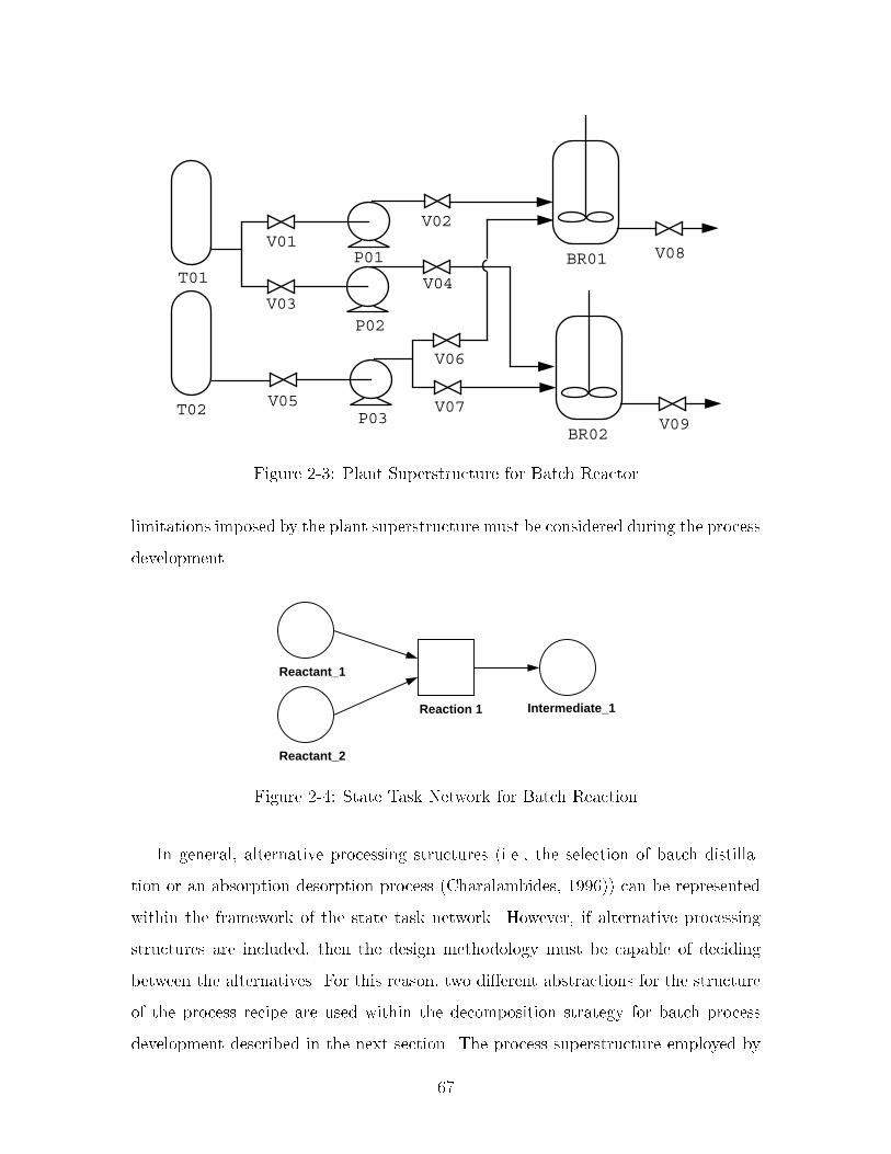
V01V02
V03V04
V05
V06
V08
T01
T02
BR01P01
P02
P03BR02
V09V07
Figure ��� Plant Superstructure for Batch Reactor
limitations imposed by the plant superstructure must be considered during the process
development
Reactant_1
Reactant_2
Reaction 1 Intermediate_1
Figure ��� State Task Network for Batch Reaction
In general� alternative processing structures �ie� the selection of batch distilla
tion or an absorption desorption process �Charalambides� ������ can be represented
within the framework of the state task network However� if alternative processing
structures are included� then the design methodology must be capable of deciding
between the alternatives For this reason� two di�erent abstractions for the structure
of the process recipe are used within the decomposition strategy for batch process
development described in the next section The process superstructure employed by
��

the screening models� which is a restricted form of state task network� provides al
ternative processing con�gurations The screening models are able to select between
these alternatives as demonstrated by the case studies in chapters � and � However�
current dynamic optimization techniques cannot select between alternative process
ing con�gurations in most cases� so the state task networks representing the process
recipe employed during the application of the dynamic optimization do not contain
alternative processing structures
The reason that the dynamic optimization techniques cannot choose between al
ternative processing con�gurations is that di�erent equations are typically required
to represent the processing operations when they are performed and when they are
idle For example� when a distillation column is operating normally the holdup of
material on the trays and in the reboiler are nonzero and the intensive properties
of the system are wellde�ned However� if the column remains idle� the holdup
of material is zero� and the intensive properties are not de�ned by the typical re
lationships Combined discrete�continuous modeling languages permit models that
consider these two cases using separate sets of equations to represent each situation�
switching between them when the appropriate conditions are satis�ed �Barton� �����
However� current dynamic optimization methods cannot handle situations when the
model equations can change implicitly Note that this situation may soon change�
in fact� recent theoretical advances de�ning the parametric sensitivities across im
plicit discontinuities �ie� state events� permit gradient based dynamic optimization
of general hybrid discrete�continuous models using control vector parameterization
�Barton� ����� In either case� the dynamic optimization problems representing the
performance subproblem employ a STN that contains the subset of the processing
alternatives that has been de�ned by the solution of the screening model
The exibility with which equipment can be assigned to processing tasks within
the screening models is similar to the equipment con�gurations considered in the
batch process scheduling literature The case studies assume that equipment units
are chosen from the inventory of equipment and reserved for the manufacture of the
desired product until the end of the campaign At the start of the campaign� a
��

pipe�tter makes the necessary connections between the processing equipment� these
connections remain in place until the campaign has been completed The case stud
ies demonstrate that the screening models can consider this level of exibility with
respect to the equipment assignment However� the equipment con�gurations avail
able within most manufacturing facilities are far more restrictive that those that have
been allowed within the screening models Although some toll manufacturers do in
fact operate in this fashion� it is only practical to connect vessels that are situated in
the same vicinity or vessels that can be easily moved Many large specialty chemical
and pharmaceutical manufacturers have far more structured and restricted equipment
con�gurations The processing equipment within their facilities is typically housed in
a number of buildings that each contain several production areas Each production
area may contain � to � production bays The production bays contain a variety of
equipment such as reactors� �lters� and storage vessels of similar size Several bays
may share some common items of equipment for drying and solvent switch operations
Large facilities may have about ��� production areas on a given site However� a much
smaller number of these may be suitable for a particular process For example� some
are reserved for high pressure operation� some for atmospheric operation or slightly
above� and other bays may not possess the equipment required for some processing
steps Thus� for a particular set of reaction steps a much smaller number of bays may
be appropriate Many of these facilities also separate the solvent recovery operations
from the reaction steps All of these restrictions can be represented as additional
constraints in the formulation presented in chapter � In summary� the combinatorial
aspects of the equipment allocation considered within this research are more than
adequate to represent the equipment options available to most manufacturers In
fact� in many cases� the exibility considered here is far greater than the situation
facing many manufacturers In particular� note that the scheduling of these processes
is far more restricted that the scheduling of blending and formulation operations�
commonly examined in the scheduling literature� where the combinatorial complexity
can be many orders of magnitude greater� but where detailed dynamic modeling is
not likely to lead to dramatic improvements in the process e�ciency �even if adequate
��

models exist�
��� Decomposition Algorithm for Batch Process
Development
The ability of the screening model to consider the discrete and the dynamic operating
decisions simultaneously and solve the resulting model to guaranteed global optimal
ity permits the derivation of a rigorous decomposition algorithm for batch process
development The algorithm employs mathematical models of the processing tasks at
two levels of detail� algebraic screening models that provide rigorous lower bounds on
the production cost� and detailed dynamic models that accurately predict the process
performance
The extension of traditional mixedinteger nonlinear programming decomposition
methods �Geo�rion� ����� Duran and Grossmann� ����� to batch process development
and to other mixed time invariant integer dynamic optimization problems is thwarted
by the inability to derive a valid Master problem using information provided by the
primal� among other problems �Allgor and Barton� ����b� However� the screening
model�s lower bounding property permits it to be employed as part of a decomposition
strategy for the solution of the mixedinteger dynamic optimization This algorithm
is discussed in chapter �
The algorithm decomposes the original process development problem into two
subproblems The solution of the �rst� the screening model� provides a lower bound
on the cost of future solutions The second subproblem is the performance subproblem
which is formulated as a dynamic optimization problem in which the discrete decision
variables in the original problem take the values determined by the solution of the
corresponding screening model� its solution yields a feasible detailed design
The screening model provides information that is either required or bene�cial for
the formulation and solution of the dynamic optimization problem that corresponds
to the performance subproblem given the allocation of the plant resources de�ned by
��

the solution of the screening model The solution of the screening model provides�
� A de�nition of the processing structure� de�ning what operations should be
included and what operations are not required
� An assignment of equipment items to the tasks that are performed These
equipment items are selected from the manufacturing facility�s inventory� and
dedicated to a particular task or set of sequential reaction tasks for the duration
of the campaign
� Information indicating which batch distillation regions are active Since the ac
tive batch distillation region is represented using a discrete variable� qualitative
changes to the performance of the distillation column resulting from feeds in
di�erent regions can be easily identi�ed
� The number of distillation cuts required under ideal conditions While more
cuts may be required in the detailed design� the number of cuts given by the
screening model provides information that can be employed to decide how many
cuts and o� cuts should be considered during the dynamic optimization
� De�nition of the basic structure of the state task network de�ning the process
for these values of the discrete decision variables
� Initial values for the compositions of the state nodes within the STN described
above The state nodes represent either recycled material or material that
decouples the dynamic interactions between processing tasks �ie� material that
leaves the reaction task and is fed to the distillation task at the start of the next
batch� The values of these states de�ned by the screening model may not be
feasible for the dynamic optimization� but they should provide a good initial
guess for the optimal values
Next� we examine how this information facilitates the formulation and solution of the
corresponding dynamic optimization problem The solution of the screening model
for the �rst case study shown in �gure �� will be used to demonstrate the points
��
Note that a mixed time invariant integer dynamic optimization formulation of this
same example is given in section ��
Since the performance of a processing task may depend on both the chosen oper
ating policies and the characteristics of the equipment in which it is carried out� the
performance subproblem requires that the equipment items assigned to each process
ing task are known In this algorithm� these assignments are �xed by the solution of
the corresponding screening model� so the appropriate dynamic model can be selected
for each task when formulating the dynamic optimization In addition� the inequal
ity path constraints may depend on the equipment assigned to the processing task
�eg� equipment over ow constraints� maximum vapor rate constraints� etc�� so the
equipment assignment must be known before the appropriate dynamic optimization
can be solved
In order to formulate the dynamic optimization subproblem� the state task net
work for the process must be de�ned We could choose to include many states and
tasks that may not be required� but this will lead to redundancy in the solutions
that may be obtained Instead� we choose to employ the information provided by
the solution of the screening model to construct a state task network for the process
that reduces the size of the resulting dynamic optimization by eliminating redundant
processing tasks� removing redundant processing tasks also improves the performance
of the optimization algorithm The key pieces of information that are required to con
struct an appropriate state task network are the number of tasks that are included
in the processing network� the number of cuts �and potential o� cuts� taken from
each of the separation tasks� and the recycle of material within the process indicat
ing where the material produced by one task is next used Once these decisions have
been made� the processing structure is determined Comparing �gure �� to �gure ��
clearly shows that the process structure de�ned by the solution of the screening model
is much simpler than the process structure that allows for all the cuts that might be
required in each of the separation tasks In fact� the screening model predicts that
only two overhead cuts are required for the �rst distillation and only one is required
for the second Without this knowledge� we would allow for �ve overhead cuts in
��

the process structure because the process contains six components Furthermore� the
recycle structure of the process is de�ned by the screening model� simplifying the
material balances around the tanks de�ning the material states Using the process
structure de�ned by the screening model allows us to eliminate redundancy in the
de�nition of the process structure which should permit the dynamic optimization al
gorithms to perform better� since all of the optimization parameters should a�ect the
objective value In contrast� including cuts that are not required will lead to multiple
solutions with the same objective value� which will probably degrade the performance
of the optimization algorithm
The dynamic optimization formulation of the performance subproblem solves for
both the operating pro�les of the processing tasks and the values characterizing the
states in the STN simultaneously In the example shown here� the temperature pro�le
in the reactor� the re ux ratio of the columns� and the split fraction determining
the distribution of ow between the two overhead cuts on the second column are
treated as the controls The composition and amount of material in each of the state
nodes generated for each batch is also determined� in �gure �� the state nodes are
represented using storage tanks that hold the material Material transfers occurring
at the beginning and end of a task are represented using the gray lines with larger
dashes� and the constraints depicting the transfer of material from one task to the next
are shown using small black dashed lines The solid lines represent material transfers
during the task Note that this picture assumes that both the reactors and columns
are operating in batch rather than fed batch mode The per unit manufacturing cost
of inspec product is minimized during the solution of the performance subproblem
By comparing the STN shown in �gure �� to that shown in �gure ��� we ob
serve that we are only considering a subset of the potential processing structures
We recognize that this may exclude better solutions� but the dynamic optimization
algorithms cannot guarantee convergence to a global optimum This implies that
the initial guess provided to our dynamic optimization procedure may have a greater
impact on the quality of the solution obtained than the number of processing struc
tures embedded in the STN The screening model provides initial guesses for all of
��
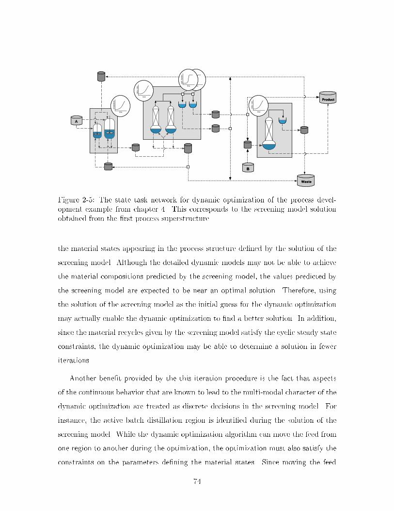
+� +�
������ ������
�
((
�
����&���� �
�
����&���� �
� ����
�
� � ������ ��
�
� � ������ ��
�
Figure ��� The state task network for dynamic optimization of the process development example from chapter � This corresponds to the screening model solutionobtained from the �rst process superstructure
the material states appearing in the process structure de�ned by the solution of the
screening model Although the detailed dynamic models may not be able to achieve
the material compositions predicted by the screening model� the values predicted by
the screening model are expected to be near an optimal solution Therefore� using
the solution of the screening model as the initial guess for the dynamic optimization
may actually enable the dynamic optimization to �nd a better solution In addition�
since the material recycles given by the screening model satisfy the cyclic steady state
constraints� the dynamic optimization may be able to determine a solution in fewer
iterations
Another bene�t provided by the this iteration procedure is the fact that aspects
of the continuous behavior that are known to lead to the multimodal character of the
dynamic optimization are treated as discrete decisions in the screening model For
instance� the active batch distillation region is identi�ed during the solution of the
screening model While the dynamic optimization algorithm can move the feed from
one region to another during the optimization� the optimization must also satisfy the
constraints on the parameters de�ning the material states Since moving the feed
��

from one region to another can change the qualitative behavior of the distillation�
the composition of the material in the accumulator at the end of the distillation
task may di�er wildly from the parameters corresponding to material in the tank fed
by the accumulator Since the optimization contains constraints that require that
the composition of the material in tank representing the state node is equal to the
material in the accumulator at the end of the task� the large di�erence in composition
will result in a large violation of this constraint The NLP solver will most likely force
the distillation feed back into the original batch distillation to reduce this constraint
violation In our algorithm� the dynamic optimization will investigate processes with
feeds in other batch distillation regions� which may also result in di�erent process
structures� during the solution of other instances of the performance subproblem
The integer cuts added to the screening model at every iteration ensure that
previously examined discrete alternatives are not revisited We treat the inclusion or
exclusion of tasks� the assignment of equipment to particular tasks� and the active
batch distillation region as the discrete variables de�ning the structure of the process
The performance subproblem is solved for each of these discrete alternatives until the
termination criterion of the algorithm is satis�ed Although we could have chosen
to regard only the assignment of equipment and the inclusion of processing tasks
in the de�nition of the discrete alternatives� we would then rely on the dynamic
optimization to �nd the best local optimum of functions that we know to be multi
modal By de�ning the discrete alternatives as we have� we account for the some of
the qualitative changes to the process performance in the discrete domain� allowing
us to determine a local optimum in each of these domains through the solution of a
di�erent instance of the performance subproblem
�� Summary
This chapter demonstrates that previous research addressing batch process develop
ment cannot simultaneously address the discrete and detailed dynamic design deci
sions in a rigorous fashion However� previous researchers have derived techniques ca
��

pable of handling subproblems encountered during batch process development These
techniques are employed within the design method proposed by this thesis For exam
ple� the decomposition algorithm for batch process development proposed within this
thesis utilizes the dynamic optimization techniques developed for the performance
subproblem and the type of equipment allocation constraints developed for the plant
design problem
The screening models introduced in this thesis permit the derivation of a rigorous
decomposition algorithm capable of addressing both the discrete and continuous de
cisions without requiring total enumeration of the discrete space This represents the
�rst rigorous approach to the solution of the batch process development problem with
the potential to avoid total enumeration of the discrete space The approach couples
insightbased targeting models with gradient based dynamic optimization algorithms
In addition� the screening models can be employed to enhance the application of ex
isting design methods The derivation of the screening models is discussed in the next
chapter
��

Chapter �
Screening Models for Batch
Process Development
Batch process development � the design of a process to manufacture a new or modi
�ed product within an existing manufacturing facility � is frequently encountered in
the specialty chemical and synthetic pharmaceutical industries Allgor et al� ������
demonstrated the importance of batch process development and stressed the need
to develop systematic methodologies that permit the rapid design of e�cient batch
processes In order to design an optimal batch process� the optimal recipe and the
allocation and scheduling of the plant�s resources must be determined simultaneously
This chapter introduces screening models for batch process development that yield
a rigorous bound on the cost of the design by considering decisions related to the
operation and scheduling of the processing tasks within a single model that can be
solved to global optimality
This chapter introduces the notion of screening models for batch process devel
opment Screening models yield a rigorous lower bound on the cost of the process�
providing both design targets and a valid way in which to prune or screen discrete
alternatives �process structures and equipment con�gurations� that cannot possibly
lead to the optimal solution These models consider changes to the process structure�
the operation of the tasks� and the allocation of equipment simultaneously In addi
tion� these models embed aspects of the process synthesis not considered in previous
��

research dealing with batch process design However� they do not provide a detailed
process design� so they must be used in conjunction with techniques that consider
the dynamics of the process in detail� such as the multistage dynamic optimization
formulations used to address the performance subproblem �Charalambides� �����
In the remainder of this chapter� we discuss the properties that must be satis�ed
by screening models and derive screening models for batch process development that
achieve these properties In the next section we discuss how information calculated
by these models can be employed to enhance existing approaches for batch process
development� and how these models facilitate a rigorous decomposition approach for
the design of these processes The application of these models to realistic process
development examples is presented in chapters � and �
��� Deriving Screening Models for Reaction�Dis�
tillation Networks
The usefulness of screening models hinges on their ability to yield a rigorous lower
bound on the cost of the process being developed To achieve this bounding property�
the models must overestimate the feasible region� underestimate the design objective�
and consider all of the optimization variables simultaneously In addition� the opti
mization procedures used to solve these models must obtain a global minimum When
these conditions are satis�ed� the solution of a screening model provides a rigorous
lower bound on solution of the original problem
In order to derive screening models with these properties� constraints related to
the equipment allocation and scheduling are expressed in their original form� but the
constraints de�ning the dynamic performance of the processing tasks are relaxed
Algebraic equations representing performance limits replace the di�erentialalgebraic
equations describing the task performance� and time averaged material balances are
enforced Therefore� the optimization algorithms used to solve the model must handle
both discrete and continuous decision variables� but need not deal with any di�erential
��

equations In the remainder of this section� we derive convex models with these
properties for the development of batch reaction�distillation networks
����� Process Abstraction
We de�ne a superstructure that embeds the synthesis alternatives considered during
the solution of the screening model The process superstructure is represented with a
directed graph consisting of state and task nodes The process is assumed to consist of
a sequence of processing trains� each train may contain a reaction and�or a separation
task Stable material is produced by every task In any train� either task may not
exist� note that the reaction tasks must exist if only one reaction pathway is considered
and the number of trains equals the number of steps in the reaction pathway A mixing
task prior to each separation task has been included in the superstructure to clarify
derivation of the model equations and simplify the notation� these tasks do not require
separate equipment items A diagram of the process superstructure is shown in �gure
�� In addition� each train of the superstructure is labeled� ordering the reaction
steps in the process Although this ordering has no impact on the superstructure at
this level of the hierarchy� it becomes important when the superstructure is re�ned
�see �gure ��� to consider the purging of recycled streams The state nodes in this
superstructure can be partitioned into two sets� nodes representing the �xed points of
a simple distillation process �����eq in �gure ���� whose composition is known before
the solution of the model� and nodes leaving the reaction and mixing tasks whose
composition is determined during the solution procedure
The superstructure looks similar to the state task networks �STN� commonly
used to represent batch processes for scheduling purposes �Kondili et al�� ������ but
it di�ers from the STN because many of the state nodes in this superstructure do
not represent material that can be found in the actual manufacturing process The
product will be manufactured in a campaign with all batches following the same
production route� so the process must operate at cyclic steady state This implies that
the arcs in the superstructure correspond to timeaveraged material ows However�
these arcs need not correspond to material transfers in the physical process For
��

eq
1
2
3
4
MixReact Distill
MixReact Distill
MixReact Distill
Waste1f
Supplyf1
Doutf
Rinf
Routf
Minf
Productf1
Figure ��� Superstructure for networks of reaction and separation tasks
instance� the targeting procedure used for the distillation tasks permits all feasible
separations to be represented in terms of convex combinations of the material sent
to each of the equilibrium point nodes The actual distillation cuts� which may
be recycled� processed further� or leave the process as waste or product� are not
represented by any single arc of the superstructure
The timeaveraged ows in the superstructure are speci�ed in terms of compo
nent molar ow rates� these ows may be speci�ed using either the pure component
or �xed point compositions as the basis The superstructure permits both splitting
and mixing of streams� but the splitting of streams leaving state nodes whose compo
sition is not known a priori is not permitted In order to enforce timeaveraged mass
balances for this superstructure� models that de�ne the timeaveraged ows leaving
the tasks in terms of the entering ows and the operating variables are required To
maintain the bounding properties of the formulation� each one of these models must
overestimate the region of the composition space that is reachable from a given in
put speci�cation Furthermore� to enforce the material balances� the models of the
reaction and distillation tasks must relate the input and outlet ows using linear
equations The following sections derive models that overestimate the composition
��

space that is reachable using batch distillation and batch reaction tasks
����� Batch Distillation Composition Bounds
The targeting model of the batch distillation tasks� coupled with the opportunities
for mixing embedded in the superstructure� must include all of the feasible sequences
of cuts that could be obtained by any batch distillation column processing the same
feed Although we recognize that separating the mixture into its pure components
represents a bound� the presence of azeotropes results in boundaries in the compo
sition space that cannot usually be crossed As a result� the sequence of products
attained from batch distillation depends on the feed composition of the mixture The
location of these boundaries is likely to a�ect the solvents and entrainers chosen� the
amount of solvent and reagent that is used� and the operation of the reactors provid
ing the feeds to the distillation columns Therefore� the targeting model must embed
these boundaries in order to generate useful information during process development
We model the distillation tasks shown in the superstructure using batch distilla
tion targeting techniques �Ahmad and Barton� ����� Ahmad and Barton� ����� to
identify the set of sharp splits that can be obtained from a given feed� we assume
that sharp splits are possible when operating under the limiting conditions and the
pot composition boundaries are linear �Ahmad and Barton� ����� We then prove
that the proposed superstructure contains all feasible sequences of cuts that can be
achieved from a given feed� including nonsharp splits and o�cuts� in spite of the fact
that we have represented distillation tasks shown in the superstructure using sharp
splits
Targeting for Sharp Splits
Simple residue curves describe the change in composition with time of an open evapo
ration process These residue curves can be placed in the composition simplex de�ned
by the pure component vectors to form a simple distillation residue curve map� an
example map for a ternary system is shown in �gure �� These curves can be de
��

�ned experimentally� or via the solution of a set of di�erential equations Doherty
and Perkins �����a� ����b� ����� showed that the pure components and azeotropes
represent the �xed points of a system of di�erential equations� further� all of the ho
mogeneous azeotropes of a given system of components can be found using established
algorithms �Fidkowski et al�� ����� We let the �xed points arranged in increasing
boiling temperature de�ne the ordered set E � f��������� � � ��epg� ep represents the
number of �xed points in the system� and �e represents the composition of each �xed
point
simpleresidue curve
•
Figure ��� Residue curve map for a ternary system with pure components ��� ���and �� The �xed point �� represents a maximum boiling binary azeotrope between�� and ��
Van Dongen and Doherty ������ compared the simple distillation residue curves
to the pot composition trajectory of a batch recti�er and demonstrated that the rec
tifying curves approach straight lines in the limit of high re ux ratio and a large
number of equilibrium stages Given a homogeneous ternary mixture under these
limiting conditions� they showed that the exact orbit of the reboiler composition and
the sequence of constantboiling product cuts can be predicted from the structure
of the residue curve map of the system Under these limiting conditions� the com
position simplex can be divided into a set of batch distillation regions Each batch
��

distillation region de�nes the set of compositions leading to the same sequence of
product cuts Figure �� shows the batch distillation regions and trajectory of the
reboiler composition for the residue curve map show in �gure ��
•
potcomposition
barrier pot compositionx
Region I
Region II
Figure ��� Ternary system with two distillation regions showing the pot compositiontrajectory for a feed in distillation region I
Ahmad and Barton ������ ����� have extended and generalized these results to
homogeneous systems with an arbitrary number of components They demonstrated
that under the assumptions of high re ux ratio� a large number of stages� and linear
pot composition boundaries� a mixture of nc components will separate into at most nc
product cuts Therefore� each batch distillation region b is represented by an ordered
subset of the �xed points� Eb� of dimension nc These batch regions cover the nc
component composition simplex
�b�B
b � Cnc � fx � Rnc � kxk� � �� xi � � �i � � � � � ncg ����
Furthermore� the members of Eb bound an nc � � dimensional simplex� termed the
product simplex The product simplex P �b� is de�ned by an nc � nc matrix Pb as
��

follows�
P �b� ��x � Cnc � x � Pb� � � � Cnc
�����
where the columns of Pb correspond to the equilibrium point compositions appearing
in the set Eb Equation ���� de�nes the barycentric coordinates � representing the
fraction of the charge appearing in each of the product cuts Every batch region b
de�nes a corresponding product simplex P �b�� but the converse is not always true
�Ahmad and Barton� ����� The targeting formulation presented here assumes that
all batch regions coincide with their corresponding product simplices� so P �b� � b
For a given mixture of components� these regions can be determined from the stability
of the �xed points �Ahmad et al�� �����
Given the product sequence de�ning each batch distillation region Eb and the
compositions of all of the �xed points �e� we only need to identify the batch distillation
region that contains the feed in order to perform the mass balance We call the region
containing the feed the active batch distillation region and identify it with the binary
variable yB Since the feed lies within the convex hull of the products of the active
region� the barycentric coordinates are positive For regions that do not contain the
feed� at least one of the barycentric coordinates is negative We permit only one region
to be active and require that the barycentric coordinates are positive ��ke � ��� so
we can express the fact that the feed composition x lies within the active region for
the distillation task in train k as follows�
Xb�B
yBkb � � � k � K ����
xk �Xb�B
yBkbXe�Eb
�ke�e � k � K ����
We derive the time averaged mass balance for the distillation task by multiplying ����
by the total feed fD We de�ne the variable fBoutb � yBb fD� to eliminate the bilinear
terms from the timeaveraged material balance and obtain the following material
��

balance for the kth distillation task�
fMout
k �Xb�B
Xe�Eb
fBoutkbe �e � k � K ����
We require that fBoutkbe � � and complete the de�nition of fBoutkbe using the following
inequality�
Xe�Eb
fBoutkbe � fmaxyBkb � k � K� b � B ����
To simplify the expressions in the rest of the model� we de�ne fDout
ke � the ow of equi
librium point e out of the distillation task k Although this constraint is redundant�
it will be eliminated during the preprocessing stage of the model �IBM� ����� and
will not e�ect the solver�s e�ciency
Xb�B
fBoutkb � fDout
k � k � K ����
The distillation targeting model presented above determines the maximum re
covery for sharp splits Now we prove that the superstructure embeds all feasible
sequences of cuts that can be obtained from the same feed Fractions of the sharp
cuts can be combined to produce any feasible combination of cuts� embedding non
sharp splits and o� cuts within the superstructure� therefore� the number of dis
tillation cuts in the actual process need not correspond to the number of cuts in
the targeting model as demonstrated in �gure �� A set of n cut compositions
S � � f�������� � � ���n � ��j � Cnc �j � � � � � ng is feasible if and only if each cut is in
the active batch distillation region ���j � B��� and the feed composition x lies within
the convex hull of the compositions in S � �x � conv�S ��� This de�nition does not
imply that these compositions can actually be achieved in a column operating with
a �nite re ux ratio Thus� the screening model embeds any o� cuts and nonsharp
splits that may be performed in the actual process
Theorem � � Given a feed composition located in a batch distillation region B with
��

linear pot composition boundaries that is identi�ed by the sequence of product composi�
tions S � f������ � � ��ncg� all sets of feasible cuts can be obtained by mixing fractions
of the cuts obtained from a column whose cut compositions are de�ned by S�
Proof� De�ne the matrix P � Rnc�nc as the matrix whose columns are the vectors
in S and the matrix P� � Rnc�n as the matrix whose columns are the vectors in S �
Since the batch distillation region is contained in the product simplex� each element
of S � can be expressed as a convex combination of the elements of S� so there exists
��j � Cnc such that ��j � P��j for every ��j � S � This de�nes the matrix ��
P� � P�� ����
Since x � conv�S ��� there exists �� � Cn such that x � P��� where ��j represents the
fraction of the charge obtained in the jth product cut of S �
x � P��� � �P����� � P������ ����
There exists � � Cnc de�ning the barycentric coordinates of the feed with respect to
the extreme points of the distillation region� x � P�� so the amounts collected in the
sharp cuts are linearly related to any feasible cuts obtained from the column
���� � � �����
This equation represents the material balance around the product cuts in the set
S It demonstrates that the amount of the cuts with the compositions in S � can be
obtained by mixing fractions of the cuts taken at the equilibrium nodes Figure ��
shows that any feasible set of cuts can be obtained from the sharp cuts determined in
the targeting model if mixing is permitted The labels on the arcs represent the time
averaged ow rates� and the labels contained in the state nodes denote the material
composition Since every element of both �� and �� is positive� all of the ows on the
arcs between the nodes are positive
��

1
2
nc
DistillationTargeting
Modelx 1
Mixer
Mixer
Mixer
Mixer
1
2
3
n
1
2
3
n
1 21
1
2
nc
n nc,n
121
Figure ��� Representation of an arbitrary distillation task by combining sharp distillation cuts and mixers
����� Reactor Targeting Model
Mass balances and reaction stoichiometry are enforced by introducing the extents of
reaction as model variables For the kth reaction task� stoichiometry is enforced by
expressing the time averaged material balance in terms of stoichiometric coe�cients
�kr and the extent �kr of reaction r
Xe�E
fRinke �e "Xr�Rk
�kr�kr � fRout � k � K �����
For components e that do not participate in reaction r of the kth reaction task�
kre � � Since the extent of the reaction is the same for all components� requiring
nonnegative ow rates insures that the reaction extents are feasible The material
balances for the reaction only constrain the feasible composition space of the reac
tions by enforcing stoichiometry and permitting no more than total conversion of any
reactant
The extents of the reaction that are achieved in the actual process depend on
the operating policies of the reaction tasks and the kinetics of the reactions Since
expressions for the reaction kinetics are available �otherwise we could not model the
reaction tasks in detail�� bounds on the achievable extents of reaction in terms of
��

key operating variables �eg� processing time� temperature� and feed composition�
can be derived and incorporated within the screening model In addition� bounds
relating the extents of competing reactions can be provided We have not derived
general expressions for these bounds since they will almost certainly depend on the
kinetics of the reactions� but the case studies presented in chapters � and � show
speci�c examples of how these bounds can be derived The case studies demonstrate
how bounds for the extents of competing reactions can be derived from the operating
temperature limits imposed on the process In addition� they demonstrate how upper
bounds on the extents can be derived from the processing time and a bound on the
temperature pro�le for the task These bounds do not exclude any feasible operating
policies� yet they manage to incorporate important tradeo�s within the screening
formulation
��� Time Averaged Material Balances
The constraints for the material balances can be derived from the superstructure�
shown in �gure ��� and the composition targeting models that relate the inlet and
outlet ow rates for the distillation and reaction task nodes in the superstructure In
fact� the material balances for the distillation and reaction tasks are shown in ����
��� and ����� respectively The screening model enforces time averaged material
balances around each of the task and state nodes in the superstructure Material
balances around the state nodes representing the �xed points of the batch distillation
regions are expressed as follows�
fSupplye "Xk�K
fDout
ke � fProducte " fWastee "
Xk�K
fRinke "Xk�K
fMin
ke � e � E �����
The following material balances around the �hypothetical� mixing tasks de�ne the
feed to the distillation tasks in terms of pure component ows
Xe�E
fMin
ke �e " fRoutk � fMout
k � k � K �����
��

Equations �������� ������ and ��������� enforce the material balances around
all of the nodes in the superstructure shown in �gure ��� these constraints denote
the material balance constraints at the highest level of the superstructure hierarchy
However� we cannot identify streams that are recycled and need to be purged by
examining the superstructure at this level of detail Since the screening models require
that a fraction of any recycled cut is purged� deriving the purge constraints requires
a more detailed view of the material ows in the process The �xed point nodes in
the superstructure shown in �gure �� are re�ned as shown in �gure �� to provide a
superstructure with more detail that identi�es recycled streams and allows them to be
purged Constraints to enforce the purge requirements require variables introduced
in the material balance constraints for the network depicted in �gure �� In general�
a hierarchy of superstructures may be used to describe the process� depending on the
type of constraints that are required
��
�
��
�
��
�
���
����
����
��
��
�� ���
�� ���
�
�� ���
�
���� �
�
�����
�������
����
��
��
����
������
�������
�
���
����
�����
��
����
����
�������
����
����
�����
���������
��������
�
�����
��
Figure ��� Detailed representation of �xed point node e used to derive the purgeconstraints
The cuts from each distillation task are sent to a splitter contained in the detailed
��

representation of the �xed point node Cuts entering the network are either sent
to waste� to product� forward in the process� or backward in the process Material
balances are derived around each node that exists in the expanded representation of
the �xed point node in ��������� Equation ����� ensures that a fraction of every
recycled stream is purged The purge fraction of each equilibrium point� Xpurgee � is
data supplied to the screening model based on engineering judgment or prior knowl
edge about trace contaminants� di�erent purge fractions can be used for each �xed
point node if desired Incorporating these constraints in the model� allows ����� to
be removed from the screening model We retain ��������� and rely on the presolver
contained in OSL to eliminate any unnecessary variables and constraints to reduce
the size of the linear programs actually solved during the branch and bound iteration
�IBM� ����� If a solver is used that does not eliminate the intermediate variables
that have been introduced here� these should be removed to reduce the size of the
models that are solved
fDout
ke � fWke " fProdke " fBke " fFke � k� e �����
fBke � f purgeke "Xk��k
fBFekk� � k� e �����
fFke �Xk��k
fBFekk� � k� e �����
fRinke " fMin
ke � fSke "Xk�
fBFek�k � k� e �����
fSupplye �Xk
fSke � e �����
fProducte � fPrgpe "Xk
fPke � e �����
fPrgwe " fPrgPe �Xk
f purgeke � e �����
Xk
fWke " fPrgwe � fWastee � e �����
f purgeke � XPurgee fBke � k� e �����
��

The supply of raw material to the process is restricted to components that can be
purchased or are available as a by product of another process within the manufactur
ing facility Let ER de�ne the set of �xed points that may be supplied to the process
and require that the feed of all other components is zero
Xe��ER
fSupplye � � �����
Finally� the product must adhere to purity speci�cations and meet manufacturing
demands The total production is given by the ow of inspec product over the entire
campaign Purity speci�cations are placed on a subset of the �xed points contained
in the product �typically these will be pure components� We let EP denote the
components whose purity in the product is speci�ed byXproduct� andQdemand represent
the manufacturing demand For example� if the desired product is component P and
it is required at �� # purity by mass� then the set EP � fPg and Xproduct � ��� The
demand and purity constraints for the manufacturing campaign are speci�ed below�
in these constraints� the time averaged ow rates denote the material ow for the
entire campaign� and the product purity is speci�ed on a mass basis
Qdemand �Xe�E
fProducte �Tew �����
XproductXe�E
fProducte we �Xe�E
�fProducte
Xe��EP
�Te �e�we�
������
The elements of w � Rnc represent the molecular weights of the pure components
We could also place restrictions on the amounts of particular impurities that are
permitted in the product For example� if the product is required at �� # purity�
but cannot contain water� then a restriction must be placed on the amount of water
that is allowed Let the parameter X impuritye denote the maximum mass fraction of
�xed point e that is permitted in the product If no special restrictions are imposed�
then X impuritye � � � Xproduct for all e � EP � and X impurity
e � � for all e � EP Let
the set EI de�ne the components whose concentration in the product is restricted
��

to remain below the limit de�ned by X impuritye Note that this set need only contain
�xed points whose fraction in the product must be restricted more than the average
impurity� such as water in the example described above
X impuritye
Xe��E
fProducte� we� �Xe��E
fProducte� �Te �e�we �e � EI �����
Screening formulations containing objective functions that depend on only the
material ows in the process can be derived using the constraints presented thus
far �however� constraints that limit the extents of the reactions that were not ex
plicitly stated should also be included� For instance� the minimum raw material
and waste disposal cost for a process that meets the production requirements or the
minimum amount of waste that can be emitted to the environment can be deter
mined We merely need to postulate the objective function� incorporate constraints
������� ���� ���� �������� and ��������� and solve the resulting mixedinteger
linear program Similar models have been used for solvent recovery targeting �Ah
mad and Barton� ����� However� to account for other production costs and the
assignment and scheduling of equipment� we need to target for the time and utility
requirements for the reaction and distillation tasks and include constraints to ac
count for the equipment assignment and scheduling Such constraints are derived in
the following sections
��� Bounding Distillation Processing Time and Util�
ity Requirements
The processing time and hot and cold utility consumption of the distillation task
impact the operating cost of the entire batch process Since the operating cost of the
process is a nondecreasing function of these variables� underestimates are required
to maintain the bounding properties of the screening model However� determining
the processing time and utility cost requires knowledge of both the re ux ratio and
the amount of material taken overhead This requires knowledge of the amount of
��

material assigned to the bottoms� fBotke � de�ned later in this section
����� Distillation Processing Time Bounds
The distillation columns employed in the process are characterized by a maximum
vapor rate at which they can operate The maximum vapor rate is based on limits
imposed by the tray and downcomer design �or packing design� that avoids entrain
ment ooding for reasonable values of the liquid rate in the column �Kister� �����
We assume that no loss of e�ciency or increase in utility cost is incurred by operat
ing at this rate We also assume that no heat integration will be performed Since
operating at the maximum vapor rate will minimize the operating time but will not
hinder separation e�ciency or increase utility cost� all columns will operate at their
maximum vapor rate
The material balance around the column is used to derive bounds on the processing
time and utility requirements The column contains product cuts c to nc at the start
of the cth product cut� at the completion of the cut� cuts c " � to nc remain The
amount and composition of the material removed is known�� so the processing time
can be calculated from the vapor and distillate rates We assume that the vapor ow
rate V is bounded by the maximum rate that can be achieved in a given column� no
assumptions are made regarding the distillate rate D� or the liquid rate L
To preserve the bounding property of the screening model� a valid underestimate
of the operating time is needed The time required to obtain each cut depends on
the amount of the cut� the vapor rate� and the re ux ratio used during the cut
To provide a lower bound� we assume that the columns assigned to the distillation
task will operate at their maximum vapor rates Although the amount of material
obtained in each product cut is given by fDoute � when more than one unit is assigned�
the amount of material processed by each column will be a fraction of fDoute In the
remainder of this section� we consider fDoute to represent the material processed by the
�None of the material assigned to the bottoms cuts is taken overhead� providing an underestimateof the time and utility requirements� However� some of the overhead cut material may leave thecolumn as an impurity in the bottoms stream� and this is addressed later in this section�
��

assigned equipment units� we adjust for units in parallel �see ������ when deriving
the constraints to determine the campaign time
The processing time for each cut� tcute � is the time required to remove the cut from
the column This time is a function of the distillate rate D and can be expressed in
terms of the vapor rate and re ux ratio R Let M represent the amount of material
collected in the accumulator during the cut �dM � Ddt� and integrate the expression
V � D�� "R� for the duration of the product cut�
Z tcute
�
V dt � V tcute �
Z fDoute
�
�� "R�M��dM �����
The relationship above holds as long as the re ux policy can be expressed as a function
of the amount collected in the accumulator during a speci�c cut If the re ux ratio is
constant over the entire cut� a simple expression for the time is obtained from �����
tcute �fDoute �� "R�
V�����
The cut time de�ned in ����� provides a valid underestimate of the processing time
for a cut if R underestimates the integral of the re ux ratio over the entire cut�
R � R fDoute
�R�M�dMfDout
e
In order to obtain an underestimate of the re ux ratio� some limiting cases are
examined First� since the column is operating at its maximum vapor ow rate� we
recognize that a minimum re ux ratio is required to provide a suitable liquid rate
for proper liquid and gas ow patterns within the column This minimum ratio may
depend on the particular column� and is required to prevent undesirable operating
phenomena Kister ������ ����� describes correlations to predict these boundaries
for tray and packed columns� so we treat these boundaries as design constraints that
cannot be violated Thus� we assume that a minimum re ux ratio for the column is
speci�ed as part of the data for the problem At the very least� any feasible operating
�Note that this relationship does not assert constant molar over�ow� The vapor rate V is themaximum vapor rate that can be achieved in any part of the column� The vapor rate at the top stagemust be less than or equal to V � so the distillate rate D must be less than or equal to V�� R��
��

policy must employ a re ux ratio that exceeds this minimum Since the equilibrium
stage models will not accurately represent the process if we operate below this mini
mum� we should also include this constraint in any dynamic optimization calculations
performed on the detailed models of the distillation tasks If no information regard
ing the purity of the overhead cuts is provided� then the tightest bounds that can
be given for the re ux ratio are those at the limit of the feasible operating regime
based on liquid gas contacting Letting Rmini represent the minimum re ux ratio of
the assigned equipment unit�
Rmini � R �
R fDout
�R�M�dM
fDout�����
An underestimate of the processing time for the distillation task is obtained by
adding the processing time for all of the overhead cuts� provided that the bottoms
stream is pure If the bottoms stream contains some impurities from the overhead
stream� then some of the material that would have been taken overhead remains
in the bottoms To account for the impurity when determining the duties for the
overhead cuts� we require that the amount of impurity that can be tolerated in the
bottoms� ��XBPk � is speci�ed for each distillation task The bottoms impurities must
be fractions of the overhead cuts� so they can be de�ned as follows�
fBIke � fBotke �k� e �����Xe
fBIke � ���XBP
k
�Xe
fBotke �k �����
Valid bounds are obtained by subtracting the time required to collect the tolerated
amount of impurity at the re ux ratio employed during the overhead cut� the opti
mization is free to select the overhead material that minimizes the processing time
as the impurity Therefore� operating column i at its minimum re ux ratio de�nes
the minimum time for one column of type i to distill the material taken overhead in
��

distillation task k
tDproc
ki � � "Rmini
Vi
Xe
fDout
ke � fBotke � fBIke �����
Of course� fBIke � � and ��������� are not needed if the bottoms streams are required
to be pure
����� Bounding the Distillation Utility Requirements
The rate of energy removal� $Q� required to condense the vapor passing through the
condenser for a process operating without losses can be expressed in terms of the heat
of vaporization of the condensate �Hvap and the re ux ratio R of the cut
$Q � �HvapD�� "R� �����
The distillate composition corresponds to one of the equilibrium points in the residue
curve map� so �Hvap is known for every cut if the material is condensed at its boiling
temperature� the enthalpy of vaporization and boiling temperature of each equilibrium
point can be provided as data to the screening model� However� we cannot assume
that all of the material that is collected overhead is condensed at the boiling point
of the �xed point because the cuts that will actually be obtained in the real column
cannot achieve the limit of perfect splits When the cuts are not sharp� a particular
�xed point will be condensed as part of a mixture� so some �xed points will be
condensed at a temperature above their normal boiling point At these elevated
temperatures� the enthalpy of vaporization is less than that at the normal boiling
point because the enthalpy of vaporization is a decreasing function of temperature
�The enthalpy of vaporization must be underestimated for the �xed points� These underestimatesmust account for the enthalpy of mixing at the boiling temperature� The maximum enthalpy ofmixing can be determined by formulating and solving a global optimization problem� The globaloptimization is solved before the screening model is posed� and the solution is treated as data in thescreening model� so �Hvap
e represents the enthalpy of vaporization at the boiling point reduced by�Hmix� In principle� global optimization techniques Adjiman et al�� � �� Maranas and Floudas�� �� Smith and Pantelides� � �� can be employed to identify �Hmix for the compositions andtemperatures considered using the enthalpy model employed during the detailed dynamic simulation�
��

�Reid et al�� ����� This implies that a lower bound on the condenser duty is not
derived by simply assuming that the collected material is condensed at its boiling
temperature and the column operates at minimum re ux However� the enthalpy of
vaporization at the boiling temperature can be used to bound the reboiler duty
We assume that material charged to the column is a liquid mixture below the
boiling temperature of the �xed points collected in the overhead cuts In order to
collect material overhead� vapor must be generated We adjust for the changes of
enthalpy upon mixing separately when underestimating the energy requirements� so
we ignore mixing e�ects here and treat the mixture as if it is ideal Let �He denote
the di�erence between the molar enthalpy of the liquid of �xed point e charged to the
column and the molar enthalpy of the vapor generated in the reboiler at some point
during the operation of the column For a column operating at constant pressure�
a lower bound on the energy supplied to the reboiler during the distillation can be
determined from the amount of material taken overhead� the heat of vaporization of
this material� and the re ux policy employed�
Xe�Ovhd
%Qke �X
e�Ovhd
Z fDoutke
�
�He�� "R�Me��dMe �����
where Me represents the amount of material collected during cut e A rigorous un
derestimate of the reboiler duty is obtained from ����� when a valid underestimate
of the integral is provided� this requires valid underestimates for �He and the re ux
ratio as functions of Me and the temperature of the reboiler A simple underestimate
of the re ux ratio is obtained by assuming that the column operates at the mini
mum re ux Rmini during the entire cut Next� we demonstrate that the enthalpy of
vaporization at the boiling temperature of the �xed points ��Hvape � provides a valid
underestimate of �He
The enthalpy of vaporization at the boiling temperature of �xed point e under
estimates the di�erence in enthalpy between the liquid of �xed point e charged to
the column and the vapor that is generated in the reboiler To prove this statement
we consider two cases� vapor that is generated below the boiling temperature� and
��
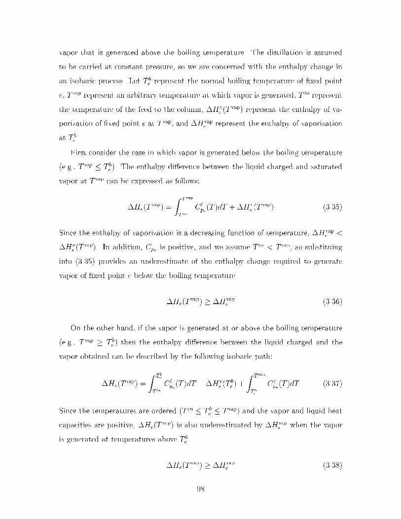
vapor that is generated above the boiling temperature The distillation is assumed
to be carried at constant pressure� so we are concerned with the enthalpy change in
an isobaric process Let T be represent the normal boiling temperature of �xed point
e� T vap represent an arbitrary temperature at which vapor is generated� T in represent
the temperature of the feed to the column� �Hve �T
vap� represent the enthalpy of va
porization of �xed point e at T vap� and �Hvape represent the enthalpy of vaporization
at T be
First consider the case in which vapor is generated below the boiling temperature
�eg� T vap � T be � The enthalpy di�erence between the liquid charged and saturated
vapor at T vap can be expressed as follows�
�He�Tvap� �
Z T vap
T inC lpe�T �dT "�Hv
e �Tvap� �����
Since the enthalpy of vaporization is a decreasing function of temperature� �Hvape �
�Hve �T
vap� In addition� Cpe is positive� and we assume T in � T vap� so substituing
into ����� provides an underestimate of the enthalpy change required to generate
vapor of �xed point e below the boiling temperature
�He�Tvap� � �Hvap
e �����
On the other hand� if the vapor is generated at or above the boiling temperature
�eg� T vap � T be � then the enthalpy di�erence between the liquid charged and the
vapor obtained can be described by the following isobaric path�
�He�Tvap� �
Z T be
T inC lpe�T �dT "�Hv
e �Tbe � "
Z T vap
T be
Cvpe�T �dT �����
Since the temperatures are ordered �T in � T be � T vap� and the vapor and liquid heat
capacities are positive� �He�Tvap� is also underestimated by �Hvap
e when the vapor
is generated at temperatures above T be
�He�Tvap� � �Hvap
e �����
��

Thus� the enthalpy of vaporization at the boiling temperature underestimates the
enthalpy di�erence between vapor at temperatures greater than T be and liquid at T in
Therefore� an underestimate of the reboiler duty of distillation k can be expressed as
follows�
Xe�Ovhd
%Qke �X
e�Ovhd�Hvap
e �� "Rmini � � k � K �����
We note that for an exothermic reactive distillation process this may not be the case�
and the heat of reaction would need to be considered when determining the bound
on the reboiler duty However� we do not consider reactive distillation in this thesis
The energy costs in this type of process are typically unimportant� so these crude
underestimates of the utility requirements do not really in uence the important design
trade o�s As mentioned in chapter �� the small energy requirements of these processes
is one of the properties that favors their manufacture in developed nations The
example problems presented in chapters � and � demonstrate that the utility costs
are insigni�cant in comparison to the other manufacturing costs In fact� these costs
would still be insigni�cant even if they were an order of magnitude greater
An underestimate of the duty for the distillation task is obtained by adding the
duties for all of the overhead cuts� provided that the bottoms stream is pure Valid
bounds are obtained by subtracting the duty required to collect the tolerated amount
of impurity at the re ux ratio employed during the overhead cut� the optimization
will select the overhead material with the greatest heat of vaporization as the impu
rity Thus� for a column operating at vapor rate of V and a constant re ux ratio R
satisfying ������ the minimum reboiler duty can be de�ned as follows�
Qk �
�� "
Xi�ID
NiXn��
yRiknRmini
�Xe
�Hvape
�fDout
ke � fBotke � fBIke
� �k � K �����
��

����� De�nition of Bottoms Cuts
Whether a separation task is performed or not is determined from the location of the
bottoms cut in the distillation task If all of the material entering the column is taken
in the bottoms� then the distillation is not performed and the processing time and
utility requirements de�ned above would both be zero Therefore� every distillation
task in the superstructure must de�ne which �xed point in the cut sequence will be
the �rst that is included in the bottoms� yBotke � � denotes that e is the �rst product
taken in the bottoms of distillation k We require a bottoms cut for every distillation
task� so
Xe�E
yBotke � � � k � K �����
and we require that the bottoms cut exists in the active batch distillation region
yBotke �Xb�Be
yBkb � e � E� k � K �����
where Be represents the set of all batch regions containing �xed point e �eg� Be �
fb � B � e � Ebg� Any cut appearing after the bottoms cut in the product sequence
will be taken in the bottoms as well� so the bottoms of the distillation task can be
de�ned as follows�
fBotke � fDout
ke
Xe��e
yBotke� � e � E� k � K �����
We require that all of the bottoms cuts are processed in the same fashion The
bottoms may be passed on to the next reaction or mixing task� or out of the process
as product or waste If the bottoms stream is comprised of only one �xed point �ie�
the last cut in the active batch distillation region�� then it may be processed in the
same way as any other cut The constraints de�ning the way that the bottoms are
���

processed are given below
Xs�S
ySks � � �k � K �����
fRink���e � fBotke ySk�rxn �k� e �����
fMin
k���e � fBotke ySk�mix �k� e �����
fProdke � fBotke ySk�prod �k� e �����
fWke � fBotke ySk�waste �k� e �����
The bottoms may only be sent anywhere if the cut is the last cut taken from the
active batch distillation region denoted by ebnc �ie� the ncth cut from the region�
ySk�any �Xb
yBkbyBotkebnc
�k �����
��� Equipment Allocation
The product will be manufactured in a single product campaign using a subset of the
equipment available within the manufacturing facility Suitable equipment items must
be assigned to all of the tasks that are performed in the process Processing tasks
can employ parallel items of equipment� but only identical columns are permitted at
the same processing stage Allocation and over ow constraints are enforced� and the
performance of the process is analyzed for two storage policies � no intermediate
storage and unlimited intermediate storage
Since a suitable item of equipment must be assigned to every task that is per
formed� we require variables to de�ne whether a task is performed Let yRxnk and zDk
de�ne the existence of reaction and distillation task k� respectively A distillation task
is performed unless the �rst cut from the active batch distillation region is included
in the bottoms Letting eb� denote the index of the �rst cut in region b� the existence
���

of the kth distillation task is de�ned as follows�
zDk � ��Xb�B
yBotkeb�yBkb � k � K �����
If a reaction task is not performed then all the extents of reaction are zero
Xr�Rk
�kr � yRxnk fmax �k �����
The screening model permits material to ow into tasks that are not performed but the
equipment over ow constraints are relaxed� so no equipment needs to be assigned For
the columns� ����� requires that all of the material leaves these tasks in the bottoms
if the distillation is not performed Equations ��������� ensure that equipment is
assigned to the reactions and distillations that are performed
Xi�IR
NiXn��
zRikn � yRxnk � k �����
Xi�ID
NiXn��
yCikn � zDk � k �����
The equipment items of type i assigned to the process cannot exceed the number of
equipment items� Ni� of that type available in the plant�s inventory
NiXn��
Xk
yRiknn � Ni � i � IR �����
NiXn��
Xk
yCiknn � Ni � i � ID �����
We also require that parallel distillation columns are the same type
Xi�ID
NiXn��
yCikn � � � k � K �����
Consecutive reaction tasks may be merged if the distillation task between them
���

is not performed� if a distillation is not performed� the optimization is free to choose
whether the adjacent reactions should be merged into the same equipment items
Let ymergek denote whether reaction k is merged with reaction k " �� zRikn denote the
whether n equipment items of type I are assigned to reaction task k� and yRikn denote
the �rst reaction task to which these equipment items are assigned
ymergek � �� zDk � k � K �����
If two consecutive reaction tasks are merged� then the same equipment items are used
for each task This implies that no new equipment items are assigned to the latter
stage which is enforced by �����
ymergek�� "
NiXn��
yRikn � � � i � IR� k � � �����
Using the fact that no new equipment is assigned� the variable zRikn can be de�ned
recursively as follows�
zRi�k���nymergek�� " yRikn � zRikn �i � IR� k � K� n �����
where zRi���n � � and ymerge� � � Equation ����� can be expressed using the following
linear constraints since zRikn � yRikn � zRi�k���nymergek�� �
zRikn � yRikn � zRk���in � k� i � IR� n �����
zRikn � yRikn � ymergek�� � k � �� i � IR� n �����
zRikn � yRikn � zRk���in " ymergek�� � � � k� i � IR� n �����
zRikn � yRikn � � � k� i � IR� n �����
Note that equations ��������� are the standard linearization proposed by Glover
������ for bilinear terms of binary variables� but ����� is required to ensure that zRikn
is equal to yRikn at the �rst stage to which equipment is assigned
���

�� Process Performance and Production Cost
The equipment assigned to the processing tasks and the storage policy selected for the
process a�ect the production rate of the process and the duration of the manufacturing
campaign Since the reaction times do not depend on the item of equipment that is
used� and identical distillation columns are assigned to the same task� an unlimited
intermediate storage policy �UIS� is modeled by treating the number of batches of
each task as an integer variable N batchRk and N batchD
k represent the number of batches
used for the reaction and distillation task in train k The number of batches for tasks
that are not performed is arbitrarily assigned to the maximum number of batches
The no intermediate storage policy �NIS� is modeled by requiring that the number of
batches used for every task is the same� and the arbitrary assignment for unperformed
tasks is relaxed The model equations below are derived for the UIS case� recognizing
that the NIS case can be derived by adding constraints� or substituting N batch for both
N batchRk and N batchD
k Letting the time averaged ows represent the total ows over
the duration of the campaign� the following constraint underestimates the processing
volume required for the reactors and represent a relaxation of the constraint requiring
that the reactors do not over ow�
Xe
fRoutke �Te v �Xi�IR
NiXn��
zRiknnNbatchRk
%Vi "NBmax
V Cmax��� yRxnk
� � k �����
where v is a vector whose components underestimate the molar volume of each of
the pure components in the process over the temperature range of interest If volume
changes upon mixing are modeled� these underestimates must be chosen so that valid
underestimates are still obtained for the resulting mixture volumes when the volume
is calculated as if it is an ideal mixture� Note that the volume requirement is based
solely on the underestimate of the �nal reaction volume in order to account for fed
�To account for volume changes� the molar volume of each component is adjusted to account forthe maximum volume change upon mixing that is possible over the temperature and compositionsconsidered� This maximum change can� in principle� be calculated by applying global optimizationtechniques Adjiman et al�� � �� Maranas and Floudas� � �� Smith and Pantelides� � �� to themathematical model used to predict liquid volume in the detailed dynamic models�
���

batch operating policies� and that the constraint is relaxed if the reaction task is
not performed and the contents are passed on to the subsequent distillation task
If the reactions must run in batch mode� then a similar constraint can be imposed
on the initial reactor volume Detailed simulation of a reactor with these feed ows
may actually over ow since these constraints overestimate the feasible region Similar
constraints are enforced for the distillation columns� but we assume that all of the
material is charged to the column at the start of the task
Xe
vT fMout
e �Xi�ID
NiXn��
nyCiknNbatchDk
%Vi "NBmax
V Cmax��� zDk
� � k �����
The campaign time for the process depends upon the processing times for the
individual tasks The processing time for each distillation task depends upon the
columns assigned and the amount of material processed Parallel distillation columns
are required to be of the same type� so an optimum exists with equal amounts of ma
terial sent to each Thus� the processing time for columns operating at the minimum
allowable re ux ratio of Rmini to complete distillation task k is given as follows�
tDk �
�Xe
fDout
ke � fBotke � fBIke
�Xi�ID
Xn�Ni
zCikn�� "Rmini �
nVi�����
The reaction processing times tRk for one batch are independent of the assigned equip
ment units� yet we need to consider whether the reaction tasks are merged to deter
mine the total batch processing time for reactors assigned to these tasks
tmergedk � tRk " ymergek�� tmergedk�� � k �����
The total processing time needs to consider the transfer times and any time allotted
to bring the columns to total re ux Constant transfer times are assumed� leading to
the following bounds on the campaign time
tcampaign � tDk "N batchDk
�tcharge " tempty " treflux
� � k �����
���

tcampaign � N batchRk
�tmergedk " tcharge " tempty
� k �����
In addition� the time available for manufacture is typically restricted
tcampaign � thorizon �����
The cost of manufacture includes raw material� waste disposal� equipment use� and
utility costs Each equipment item has associated an hourly rental charge Equipment
items must be rented for the entire campaign� so the equipment cost for the campaign
can be expressed as follows�
cequip � tcampaignXi�ID
NiXn��
nzCiknCEi " tcampaign
Xi�IR
NiXn��
nzRiknCEi �����
Utility costs are calculated from the duties for distillation tasks and cost of the spe
ci�c utility required Below� we assume only one level of the hot and cold utility is
available� although this is not necessary in general
�Chu " Ccu
�Xk
Qk � cutility �����
Raw material and waste disposal charges are associated with every �xed point node
Total waste and raw material costs are determined from the total mass of material
entering and leaving the process
craw �Xe�ER
Cref
Supplye �����
cwaste �Xe�E
Cwe f
Wastee �����
An underestimate of the total manufacturing cost is given as the sum of the individual
costs
ctotal � craw " cwaste " cutility " cequip �����
���

�� Formulating the model to be solved
The constraints presented above permit the minimization of the underestimate of
the manufacturing cost expressed in ����� subject to constraints �������� ������
���������� ���������� ���������� and ��������� However� the model� as pre
sented� cannot be solved to guaranteed global optimality since it is nonconvex All of
the nonconvexities in the formulation arise from bilinear terms between discrete vari
ables or between discrete and continuous variables� these terms are present in ������
���������� ������ ���������� ������ and ����� Since exact linearizations of these
expressions are possible� the model can be transformed into a mixedinteger linear
program that can be solved to guaranteed global optimality �Glover� ����� Adams
and Sherali� �����
The bilinear products of two binary variables are modeled by de�ning continuous
variables that are an exact linearization of the bilinear product For example� the
bilinear product yBotkeb�
yBkb appearing in ����� is replaced by introducing the continuous
variable zB�
kb equal to the bilinear product that is de�ned in terms of linear constraints
following the linearization scheme proposed by Glover �������
zB�
kb � yBotkeb�� b� k �����
zB�
kb � yBkb �b� k �����
zB�
kb � yBotkeb�" yBkb � � � b� k �����
The bilinear terms of continuous and discrete variables are also linearized following
the scheme proposed by Glover ������ that exploits the upper and lower bounds �eg�
������ on the continuous variables For example� the variable tRMk is introduced to
replace the bilinear term in �����
tmergedk � tmerged�
k ��� ymergek � � tRMk � tmergedk � tmerged�
k ��� yNn � � k � K �����
tmerged�
k ymergek � tRMk � tmerged�
k ymergek � k � K �����
tmerged�
k � tRMk � tmerged�
k �����
���

These constraints typically increase the integrality gap of the model Finding tight
upper and lower bounds on the variables helps to mitigate this e�ect� calculations
to estimate tight bounds on the variables are discussed in chapter � Additional
constraints can also be introduced to derive a tighter formulation �Adams and Sherali�
�����
The integer variables representing the number of batches are modeled as the sum
of binary variables to enable standard linearization techniques to be applied Special
ordered sets of type � are used for these binary variables to improve the e�ciency of
the solver�s branch and bound iteration �Beale and Tomlin� �����
N batch �NBmaxXm��
myNBm �����
NBmaxXm��
yNBm � � �����
��� Conclusions
Screening models for batch process development have been derived A superstructure
for networks of batch reaction�distillation tasks has been presented This super
structure embeds sequences of reaction and distillation tasks with material recycles
Equations to enforce time averaged material balances for the nodes in the superstruc
ture have been derived Composition targets for the reaction and distillation tasks
overestimate the feasible region of operation and enforce mass balances for the tasks
Although the distillation targeting model assumes sharp splits� we have demonstrated
that the superstructure embeds all feasible sequences of distillation cuts In addition�
the modeling equations for the reaction and distillation tasks provide rigorous un
derestimates of the processing time and utility requirements The distillation targets
that have been derived show that when the minimum re ux ratio is determined from
the limit required for proper gas�liquid contacting� the screening model can be cast
as a mixedinteger linear program Within this formulation� the screening models
address the allocation of equipment to processing tasks for both UIS and NIS storage
���

policies� and consider raw material� waste disposal� utility� and equipment costs
The screening models provide a rigorous lower bound on the cost of the design
This lower bound can be employed as a design target to enhance existing design
methods� or as the basis for a rigorous decomposition algorithm to address batch pro
cess development For instance� the solution of the screening model can be employed
as a metric upon which the bene�ts of design optimization can be assessed� and it
can be used to determine whether a new product has any chance of being pro�table
Screening models also enable the development of the rigorous decomposition strategy
for the improvement of the design� discussed in section ��� that has the potential
to avoid total enumeration of the discrete space The decomposition strategy also
provides a rigorous bound the distance to the global solution upon termination
In addition� the screening models consider aspects of the batch process synthesis
that have not previously been systematically addressed Solvents and reagents can
be selected from a set of candidates and the models can determine the sequence
of processing tasks from a superstructure of processing alternatives The solution
constructs not only the sequence of tasks to be performed� but also de�nes the recycle
structure for the process For these reasons� the solution provided by the screening
model provides a good starting point for detailed design This solution facilitates the
de�nition of a state task network of the process that can be used to formulate the
detailed design as a dynamic optimization problem In addition� the solution of the
screening model provides good initial guesses for the compositions and amounts of
recycled batches of material for the dynamic optimization formulation The ability to
handle discrete decisions directly within the screening model makes them particularly
appropriate for making decisions such as in which batch distillation region should the
feed to the column be located� and what equipment should be assigned to a particular
processing task
The screening models are demonstrated on two case studies in chapters � and �
���

�� Notation
����� Indexed Sets
B The set of all batch distillation regions
Be The set of all batch distillation regions containing �xed point e Be � fb �B � e � Ebg� so Be � B
E The set of all �xed points �azeotropes and pure components� in the system
EI The set of all �xed points whose maximum composition in the product is
limited �ie� impurities�� EI � E
EP The set of all �xed points regarded as product species� EP � E
ER The set of all �xed points that may be supplied to the process� ER � E
Eb The sequence of �xed points de�ning the sharp splits from batch distillation
region b
I The set of equipment types available in the manufacturing facility
ID Set of equipment types suitable for distillation tasks ID I
IR Set of equipment types suitable for reaction tasks IR I
K The set of processing trains
Rk set of reactions occurring in the reaction task in processing train k r �
�� � � � NRk
S The set de�ning the destination of the bottoms cuts S �
frxn�mix�waste� prod� anyg� indicating whether the bottoms are sent to
the next reaction task� to the next mixing task� to waste� to product� or to
anywhere in the process
����� Integer Variables
N batchDk number of batches used for the distillation task k
N batchRk number of batches used for the reaction task k
����� Binary Variables
yBkb Is region b the active batch region for distillation k
���

yBotke Is �xed point e the �rst �xed point appearing in the bottoms of distillation
k
yCkin Are n units of type i is assigned to distillation task k
ymergek Is reaction task k is merged with reaction task k " �
yRikn Do n reactors of type i begin processing potentially merged reaction tasks
at stage k
yRxnk Is reaction task k is performed
ySks Are the bottoms from distillation k are sent to s
����� Exact linearizations of bilinear products of binary vari
ables
zDk Is distillation k is performed
zRikn Are n reactors of type i are employed for reaction task k
���� Continuous Variables
cequip equipment cost for the manufacturing campaign
craw raw material cost for the manufacturing campaign
ctotal total manufacturing cost
cutility utility cost for the manufacturing campaign
cwaste waste disposal cost for the manufacturing campaign
fBke ow from splitter node k to the corresponding backward node within the
expanded representation of �xed point e
fBFekk� time averaged ow of �xed point e from distillation k to reactors and
mixers at stage k�
fBIke total ow of overhead species e that could be contained in the bottoms
of distillation k as an impurity
fBotke total ow of �xed point e taken in the bottoms of distillation k
fBoutkbe time averaged ow of the �xed point e out of distillation k in batch
region b
���

fDout
ke time averaged ow of the �xed point e out of distillation k
fFke ow of �xed point e from distillation k that is sent forward in the process
for further processing
fMin
ke the time averaged ow of �xed point e into mixer k
fMout
k the time averaged component ows into distillation k� fMout
k � Rnc
fProducte the time averaged ow rate of �xed point e in product
fPke ow from splitter node k to the product node within the expanded rep
resentation of �xed point e
fPrgwe total ow of �xed point e purged from recycle streams that leaves the
process as waste
fPrgpe total ow of �xed point e purged from recycle streams that leaves the
process in the product stream
f purgeke recycled ow of �xed point e from distillation k that must be purged
from the process
fRinke the time averaged ow of �xed point e into the reactor train k
fSke total ow of �xed point e into the process that is sent to reactors and
mixers in processing train k
fSupplye the time averaged supply of �xed point e
fWke ow from splitter node k to the waste node within the expanded repre
sentation of �xed point e
fWastee the time averaged waste ow of �xed point e
Qk condenser duty
tcampaign total length of the manufacturing campaign
tDk processing time for distillation task k
tmergedk total processing time for any merged reaction tasks ending with stage k
tRk processing time for reaction task k
� The barycentric coordinates� � � Rnc
�kr the extent of reaction r in reaction task k
���

����� Parameters
Ccu cost of cold utility per unit energy
CEi rental rate for equipment unit i
Chu cost of hot utility per unit energy
Cre cost to purchase a unit mass of �xed point e
Cwe cost to dispose of a unit mass of �xed point e
fmax upper bound for time averaged ows in the process
Ni number of equipment units i in the manufacturing facility
NBmaxmaximum number of batches that may be employed during the campaign
Qdemand product demand
Rmini the minimum re ux ratio for proper gas�liquid contacting in distillation
column i
tcharge time required to charge one batch of material to an equipment unit
tempty time required to empty one batch of material from an equipment unit
thorizon horizon time for manufacture
treflux time required to bring a column to total re ux
ve underestimate of the molar volume of equilibrium point e at processing
conditions
%Vi processing volume of equipment unit i
Vi maximum vapor rate for distillation column i � ID
we molecular weight of equilibrium point e
�Hvape underestimate of the heat of vaporization of equilibrium point e at the
at the processing conditions
�e composition of �xed point e
�kr the stoichiometric coe�cients for reaction r in reaction task k
���

���

Chapter �
Using Screening Models to Identify
Favorable Processing Structures
The ability of screening models to discriminate between alternative process structures
is demonstrated on a simple batch process development problem Although only one
reaction step is required in this process� the complexity of the chemistry and the
thermodynamics is such that the interaction between operation of the separation and
reaction tasks leads to a large set of alternative con�gurations for the state task
network de�ning the process The screening model automatically selects attractive
alternatives meeting the design constraints� allowing the engineer to focus on the
detailed design of these con�gurations This example clearly shows the importance
of quickly identifying the most attractive alternatives in order to avoid wasting time
and e�ort optimizing designs resulting from poor synthesis decisions Incorporating
the dominant operating tradeo�s within the algebraic bounding models is the key
to deriving an e�ective screening model for the process This process demonstrates
the type of processing tradeo�s that are important during the optimization of batch
reaction�distillation networks� yet the level of detail has been minimized to highlight
the speci�c tradeo�s exploited during the synthesis and to simplify the analysis of
the resulting design
The process examined consists of a sequence of competing �rst order reactions
This example also demonstrates how bounds for the extents of reaction in terms of
���

key processing variables can be derived
��� Process Description
The process examined consists of a competing set of reactions that convert the raw
materials to both the desired product �P � and waste materials �W��W�� The product
can be separated by distillation The bench scale synthesis employed a simple two
stage reaction�distillation process� but made use of an ice bath not available in the
existing manufacturing facility The reaction step comprises the set of competing
reactions shown in ���� All of the reactions are �rst order in either A or I at the
conditions under which the process may be operated Any of the components B� W��
or W� can be used to solvate the reactions
A "B�� I
�� Py�
y�
W� W�
����
The relative rates of the reactions have been chosen so that they agree with an early
study of reaction temperature optimization �Denbigh� ������ the reaction rates follow
Arrhenius rate expressions according to the constants listed in table �� All of the
reactions are catalyzed by the same catalyst� and we assume that enough catalyst is
present for the rate expressions to remain accurate Degradation of the catalyst is
not considered
k EA
Reaction s�� Jmol
� ��� ������ ��� ������ ��� ������ ���� �����
Table ��� Constants for the Arrhenius rate expressions for the �rst order reaction
rates �ri � Cikie�EART �
���

The process considered contains the six components shown in ���� These compo
nents form one ternary and two binary azeotropes The azeotropes are all contained
on the facet of the composition simplex formed by B� W�� and P shown in �gure
�� The composition ��e� of each azeotrope is shown in table �� These azeotropes
divide the composition space into the �ve batch distillation whose product sequences
are shown in table ��
Azeotrope Compositionp W�P BW�P BW�
B ��� ��� ���W� ��� ��� ���P ��� ��� ���
Table ��� Azeotrope compositions for the three azeotropes formed between B� W��and P
b Product sequence
� f A� W��P � W�� I� B�W�� W� g� f A� W��P � B�W��P � I� B�W�� W� g� f B� A� B�W��P � I� B�W�� W� g� f B� A� B�W��P � I� P � W� g� f A� W��P � B�W��P � I� P � W� g
Table ��� Product cut sequences for the distillation regions
��� Design Constraints
The equipment and utilities available within the manufacturing facility impose con
straints on the design of the manufacturing process that often do not exist at the
laboratory scale �Allgor et al�� ����� Other design constraints may be imposed in
order to adhere to environmental and safety regulations or to ensure the proper op
eration of particular tasks �ie� temperature constraints to avoid undesirable side
reactions and�or thermal runaway� These constraints must be addressed during pro
���

����
��
�
��
��������
������
������
������ �������
�������
�
���������
Figure ��� Distillation regions projected onto the facet formed by B� W�� and P
cess development Imposing these restrictions may complicate the engineer�s goal of
rapidly designing an e�cient process by requiring the engineer to focus much of his
or her e�ort on satisfying the constraints However� the design constraints such as
emission limits� solvent to reactant ratios� conversion requirements� and temperature
bounds are easily embedded within the screening models Furthermore� these con
straints are exploited during the development of the screening models themselves and
actually aid in the derivation of targets for the reaction tasks
In this example� the manufacturing facility�s utility system limits the tempera
tures that may be employed during the operation of the tasks Since the only cold
utility is cooling water which is available at ��� K� the bench scale policy of run
ning the reaction in an ice bath cannot be implemented in the manufacturing facility
The manufacturing facility�s equipment requires that the reactions are conducted at
atmospheric pressure� so the maximum reaction temperature cannot exceed either
the onset temperature for thermal runaway �eg� decomposition�polymerization� ad
justed by a safety factor� or the greatest boiling temperature of any of the �xed points
of the residue curve map �W�� However� these temperature restrictions enable the
���

derivation of bounds for the extents and selectivity of the competing reactions
In addition� design constraints are imposed to ensure proper operation of the
reactions A molar ratio of solvent to reactant �either A or I� of at least �� is
required to ensure proper solvation of the reactions� and an excess of B �two times A�
are required to maintain the desired reaction kinetics These constraints are captured
in equations �������
Xe
fRinke ��Te �B " �Te �W�" �Te �W�
� � ���fRinkA " fRinkI
� �k ����
Xe
fRinke �Te �B � �fRinkA �k ����
Since the product will be processed in an existing manufacturing facility� the choice
of equipment is limited The inventory and cost of the available equipment are shown
in table ��� all of the columns contain � theoretical stages and must operate at a
re ux ratio above �� for proper gas�liquid contacting We require that distillation
columns operated in parallel at a stage are identical
ReactorsVolume Available Rental Rate&m�' Units & � � hr'� � ��� � ��� � ��
Distillation ColumnsVolume Vapor Rate Available Rental Rate&m�' &kmol�hr' Units & � � hr'� �� � ��� �� � ���� �� � ���
Table ��� Inventory and rental rates for processing equipment
In order to evaluate the cost of manufacture� the raw material and waste disposal
costs are required In addition� in order to evaluate the utility costs and volume
requirements underestimates of the heat of vaporization and the molar volume is
���

required for all of the �xed points These data are provided in table �� Note that
the waste disposal costs are merely estimates based on the average waste disposal costs
for organic chemicals that are not highly toxic Of course the most accurate data that
is available should be employed� yet these �gures should provide the tradeo�s similar
to those that would be encountered by a manufacturer
Fixed Raw Waste MolarPoints Material Removal Hvap Volume Molecular
e & ��kg ' & ��kg ' &J�mol' & l�kmol ' WeightB ��� ���� ����� ����� ����A ��� ���� ����� ������ �����
W�P ���� ����� ������ �����W� ���� ����� ������ �����
BW�P ���� ����� ������ �����I ���� ����� ������ �����
BW� ���� ����� ������ �����P ���� ����� ������ �����W� ���� ����� ������ �����
Table ��� Material cost� disposal cost� and physical property data for the �xed points
��� Reaction targets
The screening model presented in chapter � enforces the mass balances around the
reactors in terms of the extents of the reactions However� to capture the dominant
operating tradeo�s related to the reaction tasks within the screening model� tighter
bounds on the extents of reaction in terms of the operating variables must be provided
In this section� bounds for the extents of the reactions shown in ���� are derived in
terms of the processing time and a bound on the temperature pro�le employed during
the reaction task These reaction targets capture key tradeo�s between the extent of
reaction� selectivity� processing time� and the reactor temperature pro�le� yet these
targets do not eliminate any portions of the feasible operating space
���

����� Bounding the selectivity and extent of reaction
First� we obtain bounds on the selectivity of competing reactions Since the selectivity
of I to W� and the selectivity of P to W� depend on only the operating temperature
pro�le� we relax the restriction that reactions � and � occur at the same temperature
as reactions � and � to derive valid bounds on the selectivity The reaction kinetics
dictate that the extreme values of the selectivity are achieved at the limits of the fea
sible temperature range For instance� the selectivity of reaction � to � is maximized
at the minimum temperature� and the converse is true for reactions � and � Upper
and lower bounds on the selectivity of the competing reactions are obtained in ����
and ���� by relating the extents of the competing reactions to the limits imposed on
the operating temperature
��k�k�eE��E�RTmax � �� � ��
k�k�eE��E�RTmin ����
��k�k�eE��E�RTmin � �� � ��
k�k�eE��E�RTmax ����
These constraints provide valid bounds on the attainable selectivity� but employ a
very crude bound on the temperature pro�le
Bounds for the extents of reaction in terms of the processing time are also easily
derived for ���� Since the reaction rates are greatest at the maximum temperature
of operation� the extents that can be achieved are less than the extents that would
be achieved if the process operated at the maximum rate The maximum extents
of reaction are achieved when all the reactants are available at the initial time� and
the reactor is operated at the maximum temperature The solution of following
di�erential equations de�nes the extents of reaction in the isothermal case�
d��max� " �max
� �
dt� max
�� NA ����
d��max� " �max
� �
dt� max
�� NI ����
The solution of ������� is de�ned by the following algebraic expressions relating the
���

maximum extents of the competing reactions to the processing time when NoA � fRinA
and NoI � fRinI ���
�� " �� � fRinA ��� e��max�� t� ����
�� " �� � �fRinI " ������ e��max�� t� ����
where
max�� � k�e
�EA�RTmax " k�e
�EA�RTmax �����
max�� � k�e
�EA�RTmax " k�e
�EA�RTmax �����
Equation ���� assumes that all of the reactant I is available at the start of the reaction
task in order to preserve the bounding property of the model Note� however� that
���� and ���� are nonlinear� and that they de�ne a nonconvex feasible region Convex
overestimates are developed for these constraints in section ���
Equations ������� provide valid bounds� but they are not likely to be very tight
because the constraint requiring that the same temperature determines both the se
lectivity and the reaction rate has been entirely relaxed In order to tighten these
bounds� we have to capture the time�temperature dependence of the operating policy
within the targeting model Incorporating the time�temperature dependence within
the screening model is di�cult because we are attempting to represent dynamic oper
ating decisions using algebraic constraints However� we can represent a bound on the
feasible temperature pro�le using algebraic constraints Furthermore� this represen
tation allows us to employ the same bounds on the extents of reactions derived above
The key is to represent the total amount of time the reaction task operates within a
given temperature range� we do not consider in what order the reactor spends time in
each of these temperature intervals or do we require that times spent in each interval
correspond to some continuous temperature pro�le The feasible temperature range
is divided into nj intervals indexed by the set J Let Tj de�ne the maximum tem
perature in each interval� where Tmin � T� � T� � � � � � Tnj � Tmax The time that
���

the reaction task operates in temperature interval j is given by tj� and the extent of
reaction that is achieved in each of these intervals is speci�ed by �Tkrj� The selectivity
targets previously derived are enforced over each of these temperature intervals
�T�jk�k�eE��E�RTj � �T�j � �T�j
k�k�eE��E�RTj�� �j � �� nj �����
�T�jk�k�eE��E�RTj�� � �T�j � �T�j
k�k�eE��E�RTj �j � �� nj �����
The bounds on the extent of reaction that can be achieved in a given time are also
enforced over each interval
�T�j " �T�j � fRinA ��� e����TjtTj � �j � �� nj �����
�T�j " �T�j � �fRinI " ������ e����TjtTj � �j � �� nj �����
where
���Tj� � k�e�EA�RTj " k�e
�EA�RTj �����
���Tj� � k�e�EA�RTj " k�e
�EA�RTj �����
Since we do not account for the order in which the reactor spends time in each of
the intervals� we have to assume that each interval is active when the concentrations
are highest in order to preserve the bounding property of the screening model Thus�
we have assumed that reaction � occurs instantaneously when calculating the rates
of reactions � and � However� the extent that can be achieved over a sequence of
intervals must be less than the extent that could be achieved if the entire reaction was
carried out in the last of these intervals This is because the maximum extents are
achieved over these intervals if all the raw materials are available at the initial time
and the reactor operates for the duration of the time spent in all of these intervals
�P
j��j tTj � at the maximum temperature contained in all of these j intervals �Tj�
�The �Tkrj de�ne the extent of reaction r occurring at processing stage k due to the time spentin temperature interval j� However� to simplify the notation we have dropped the subscript kthroughout the following sections�
���

Therefore� the following constraints are also enforced
Xj��j
�T�j� " �T�j� � fRinA ��� e����Tj
Pj��j t
Tj� � �j � �� nj �����
Xj��j
�T�j� " �T�j� � �fRinI " ������ e����Tj
Pj��j t
Tj� � �j � �� nj �����
Constraints ��������� are equivalent to ������� when the sum is taken over all
of the temperature intervals �ie� j � nj�� therefore� ������� need not be included
in the optimization model Note that ��������� provide a tighter bound on the
actual operation of the reactor than ������� because these constraints account for
the fact that the reactions must proceed at a slower rate when not operating in the
maximum temperature interval In fact� since ��������� are equivalent to �������
when j � nj and the constraints for other values of j are not necessarily inactive�
��������� de�ne a smaller feasible region and are tighter The operating time for
the reaction task and the extents of reaction are obtained by adding the contributions
from each of the temperature intervals
Xj
tTj � t � j � �� nj �����
Xj
�Trj � �r � r� j � �� nj �����
The nonlinear inequalities ������������� and ��������� require linear convex over
estimators in order to formulate the screening model for this example as an MILP
Linear overestimates of these regions are provided in section ���
����� Convexifying the Extent�Time Boundaries
Although the equations de�ning the bounds for the extents of reactions to ��������
���������� and ������������� de�ne a feasible region that appears to be convex
on �rst sight �the region under the surface shown in �gure �� appears convex��
the eigenvalues of the Hessian of these functions demonstrate quite clearly that the
expressions on the right hand sides of these inequalities are not concave All of the
���

00.5
11.5
2
0246810
0
1
2
3
4
5
6
7
8
9
10
t ff *
(1−
exp(
−k
t))
Figure ��� Surface de�ning the upper bound on the extents of reaction given byf��� e��t�
expressions on the right hand side have the form f���e��t� where f and t are positive
variables The Hessian of this expression is given below�
H � r�f��� e��t� �
�� � e��t
e��t f �e��t
� �����
The Hessian has the following eigenvalues�
�� � ��
�e��t
�f � "
pf � � " �
�� � ��
�e��t
�f � �
pf � � " �
�����
Since the eigenvalues di�er in sign� the functions de�ning the surface are not concave
and the region under the surface is not convex Therefore� tangents to the surface do
not overestimate the function over the entire space Examining the tangents of the
surface taken at larger values of f and t shows that these planes lie above surface at
all larger values of f and t� but cross the function at smaller� yet positive� values of
both f and t Examining the intersection of the tangent planes with the f t plane
shows that the line of intersection crosses through the positive orthant of the f t
plane Two strategies have been investigated to overestimate these functions with
linear constraints
The �rst method de�nes planes that do not cut o� any portions of the feasible
region that are parallel to the tangent planes Let L and M de�ne index sets used to
���

specify points � %fl� %tjm�� at which the tangents to the function are evaluated Hence�
there exists a positive constant representing the displacement Cl�m for each of the
tangent planes that de�nes a parallel plane that touches the surface at only one point
and will overestimate it at all other points in the feasible space �f � �� t � �� There
exists a point �f � �� t � �� �the sole point of contact of the displaced plane� for
which the following equation uniquely de�nes the constant Cl�m that corresponds to
the point � %fl� %tjm� at which gradient of the surface has been evaluated�
f��� e���tjm
" %fl e
���tjm �t� %tjm�" Cl�m � f
��� e��t
������
In this case� �f� t� is the sole point at which the parallel plane contacts the constraint
surface From the shape of the surface and the slope of the tangent planes� it can be
seen that the single point of contact for the parallel planes is the origin Essentially�
the displacement ensures that the intersection between the tangent plane and the f t
plane does not cross the positive orthant Setting the right hand side to zero uniquely
de�nes the constant Cl�m as shown below�
Cl�m � %fl %tjme���tjm �����
Displacing the tangent planes of the constraint surface by the amount Cl�m pro
vides linear constraints that overestimate the feasible region This strategy can be
applied to ��������� to derive linear constraints that overestimate the feasible re
gion Let the sets %fAl and %f Il de�ne the values of fRinA and�fRinI " ��
�at which the
tangents to the functions appearing on the right hand sides of ����� and ����� are
evaluated The following constraints correspond to ���������� where %fAl and %f Il rep
resent �xed values of the input ows and %tjm is a time at which the gradients have
been evaluated�
�The hat notation has been employed throughout this chapter to distinguish the constants usedto de�ne the interval boundaries from the subscripted variables appearing in the model�
���

�T�j " �T�j � fRinA
��� e����Tj�tjm
" %fAl ���Tj�e
����Tj�tjmtTj �j � J� l � L�m �M �����
�T�j " �T�j ��fRinI " ��
� ��� e����Tj �tjm
" %f Il ���Tj�e
����Tj�tjmtTj �j � J� l � L�m �M �����
A similar strategy is employed to derive a linear overestimate of the feasible region
for ���������
The addition of these constraints does not require the introduction of any addi
tional integer variables� but these constraints may not be very tight In fact� these con
straints do not even provide a tight approximation near the points � %fAl � %tjm� There
fore� we have also considered another linearization strategy that employs additional
binary variables� but leads to a tighter approximation of the nonlinear constraints
The second linearization strategy is based on the fact that ��������� and �����
���� de�ne a convex feasible region if either the reagent feeds �fRinA and fRinI " ���
or the processing time in the given temperature interval tTj is �xed Overestimating
the feed ows to a particular reaction task overestimates the feasible region for all
values in time Therefore� if fRinA � %fAl then the tangent of %fAl
��� e����Tj�tjm
overestimates the original feasible region�
�T�j " �T�j � fRinA
��� e����Tjt
Tj
� %fAl
��� e����Tj�tjm
" %fAl ���Tj�e
����Tj�tjm �tTj � %tjm� �����
The extents of reactions � and � can be related to the feed of A and the fractional
conversion of A We introduce the fractional conversion of the reactants A �x���
and I �x��� as new variables The fractional conversions account for the time and
temperature dependence of the reactions� and the fractional conversions x�� and x��
of a batch reaction operating at temperature Tj are de�ned by the following concave
���

expressions of time�
x��j � �� e����Tjtj � j �����
x��j � �� e����Tjtj � j �����
�����
Since ����� and ����� de�ne concave functions of time for temperature Tj� tangents
to these curves de�ne upper bounds on the maximum conversion of A and I that can
be achieved in a given temperature interval Thus� upper bounds on x��j and x��j are
de�ned as follows�
x��j ���� e����Tj�tjm
" ���Tj�e
����Tj�tjm �tTj � %tjm� �j � J�m �M �����
x��j ���� e����Tj�tjm
" ���Tj�e
����Tj�tjm �tTj � %tjm� �j � J�m �M �����
By bounding the fractional conversion according to ����� and ������ the feasible
region for the extents of reaction de�ned in ��������� can be overestimated using
these new variables as follows�
�T�j " ��j � fRinA x��j �j � J �����
�T�j " ��j ��fRinI " ��
�x��j �j � J �����
Equations ����� and ����� both contain bilinear terms comprised of continuous
variables However� we can employ the linear expressions providing upper bounds
on bilinear terms proposed by McCormick ������� which provide the following linear
upper bounds on fx�
fx � fLOx " fxUP � fLOxUP �����
fx � fUPx" fxLO � fUPxLO �����
where fUP and fLO provide rigorous upper and lower bounds on f � xUP and xLO
���

provide rigorous upper and lower bounds on x The only rigorous lower bound on x��j
and x��j is zero because tTj could equal zero� so ����� applied to ����� provides the
same constraint as ����� However� if we can provide a nonzero bound for fLO� we
can employ ����� to derive tighter upper bounds on the extent of reaction that can
be achieved
To apply ����� and ����� bounds on the fRinA � fRinI " ��� and on x��j and x��j are
required Upper and lower bounds on x��j and x��j of one and zero are assumed To
provide tight bounds on the feeds to the reaction tasks �xed values of the feed ows
are selected so that they de�ne an ordered set indexed by l that covers the feasible
region of feed ows �ie� � � %fAo � %fA� � � � � %fAnl �%fmax�� the values of %fAl�� and %fAl
can be thought to de�ne the upper and lower bounds of a feed interval The binary
variable yFAl is introduced to identify the feed interval in which the feed lies �ie�
%fAl�� � fRinA � %fAl � A similar set of values %f Il and binary variables yFIl are de�ned for
reactions � and � These binary variables represent SOS� sets� and are de�ned by
the following linear constraints�
Xl�L
yFAl � � �����
Xl�L
yFIl � � �����
Xl�L
%fAl��yFAl � fRinA �
Xl�L
%fAl yFAl �����
Xl�L
%f Il��yFIl � fRinI " �� �
Xl�L
%f Il yFIl �����
The upper � %fAl � and lower � %fAl��� bounds on the ows are valid if the feed interval is
active �ie� yFAl � ��� so we can derive bilinear constraints that enforce bounds on
the extents of reaction that can be achieved in a given temperature interval in terms
�An SOS� set is a set of binary variables with a natural ordering in which one member takesvalue � and all the others are �� Branch and bound algorithms can take advantage of the structureof these sets during the branching procedure Beale and Tomlin� � ����
���

of the reagent feed and the time spent in the temperature interval
yFAl��T�j " �T�j
� � %fAl��yFAl x��j � %fAl��y
FAl " yFAl fRinA �j � J� l � L �����
yFAl��T�j " �T�j
� � %fAl x��j �j � J� l � L �����
Similar constraints can be derived for reactions � and � The exact linearization
proposed by Glover ������ can be used to transform the bilinear terms appearing
����� and ����� into an equivalent set of linear constraints� To employ this strat
egy the variables (�T�jl � �T�jyFAl are introduced to denote the extent of reaction � in
temperature interval j and feed interval l In addition� the variables (x��jl � x��j yFAl �
(fRinAl � yFAl fRinA � and (fRinIl � yFIl �fRinI " ��� are introduced The same procedure is
applied for reactions � and � Note thatP
l�L (�Trjl � �Trj � j� rBounds on the (�Trjl are derived by substituting the variables for the bilinear terms
into ����� and ������ yielding the following�
(�T�jl "(�T�jl � %fAl��(x
��jl � %fAl��y
FAl " (fRinAl �j � J� l � L �����
(�T�jl "(�T�jl � %fAl x
��j �j � J� l � L �����
(�T�jl "(�T�jl � %f Il��(x
��jl � %f Il��y
FIl " (fRinIl �j � J� l � L �����
(�T�jl "(�T�jl � %f Il x
��j �j � J� l � L �����
The constraints ��������� overestimate the feasible region de�ned by the nonlinear
nonconvex constraints ��������� We can bound the region de�ned by ���������
in a similar fashion First� variables x��S
j and x��S
j are de�ned to represent the total
of x��j and x��j that can be achieved in all the temperature intervals up to j�
x��S
j �Xj��j
x��j� �j � J �����
x��S
j �Xj��j
x��j� �j � J �����
�Section ����� discusses the linearization of the bilinear terms between continuous and binaryvariables�
���

x��S
j ���� e����Tj�tjm
" ���Tj�e
����Tj�tjm�Xj��j
tTj� � %tjm
��j � J�m �M
�����
x��S
j ���� e����Tj�tjm
" ���Tj�e
����Tj�tjm�Xj��j
tTj� � %tjm
��j � J�m �M
�����
By de�ning (x��S
jl � yFAl x��S
j and (x��S
jl � yFIl x��S
j � we can derive constraints that over
estimate the feasible region de�ned by ��������� as follows�
Xj��j
�(�T�j�l "
(�T�j�l
� %fAl��(x
��S
jl � %fAl��yFAl " (fRinAl �j � J� l � L �����
Xj��j
�(�T�j�l " (�T�j�l
� %fAl x
��S
j �j � J� l � L �����
Xj��j
�(�T�j�l "
(�T�j�l
� %f Il��(x
��S
jl � %f Il��yFIl " (fRinIl �j � J� l � L �����
Xj��j
�(�T�j�l "
(�T�j�l
� %f Il x
��S
j �j � J� l � L �����
Comparison of Convexi�cation Strategies
The second strategy requires the addition of two SOS� sets of size nl �yFA and yFI� for
each reactor included in the superstructure The second strategy also introduces the
continuous variables (�Trjl�(fRinAl � (fRinIl � (x��j � (x��j � (x��
S
jl � and (x��S
jl which were not required
for the �rst linearization strategy However� the second strategy provides a tighter
linearization than the �rst Furthermore� the linearization provided by the second
strategy can be made to approximate the original constraints as tight as is desired by
increasing the sizes of the SOS� sets This is not possible with the �rst strategy
The e�ort required to solve the problem given by the second linearization strategy
was on the same order as the time required to solve the �rst The objective calculated
using the second strategy was greater than that calculated by the �rst� demonstrating
the fact that the approximation is tighter
The solutions that are presented in section �� employ the second convexi�cation
���

strategy
����� Minimum Extents of Reaction
The targets derived above capture the e�ects that modi�cations to the processing
time and the temperature pro�le have on the selectivity and the maximum extent
that can be achieved Even though the reactions may be terminated by �ltering out
the catalyst� we have not placed lower bounds on the conversion that must be achieved
in a given amount of time In fact� with only these constraints� the solution of the
screening model chooses to run the �rst two reactions to completion� separate the I�
react the I to form product in the absence of W�� and separate the product With
such a scheme� none of the product is lost in an azeotrope� making this alternative
highly attractive in the screening formulation Clearly� we would like the screening
model to incorporate a lower bound on the extents of the third and fourth reactions
to capture the fact that the �rst two reactions cannot be run to completion without
producing some W� and P in the process Such constraints are derived below
A lower bound on the extent of the third and fourth reactions can be derived by
underestimating both the rate of conversion of I and the amount of I that is available
for reaction The amount of I available for reaction can either be produced from the
reaction of A� or it may be charged directly to the reactor Since the reaction of I
is a �rst order process� the extents of reactions � and � coming from each source can
be treated separately� whether I is generated or charged� it obeys a �rst order decay�
so the conversion of a given charge of I is a function of only time since the charge
and the reaction temperature Let �I�� represent the extent of reactions � and � that
results from I fed directly to the reactor and let �A�� represent the extent of reactions
� and � resulting from the conversion of A fed to the reactor
�� " �� � �I�� " �A�� �����
Since semibatch operation is permitted� �I�� could be zero because all of the I could
be charged at the end of the reaction� yet �� " �� � �A�� We focus on determining a
���

lower bound on �A�� We know that �A�� cannot be zero for nonzero values of �� because
the rates of the �rst two reactions are �nite� so the reactor operates for a period of
time when I is present
The �rst reaction must proceed for a certain amount of time in order to achieve
a given conversion� even if the reaction proceeds at the maximum rate As I is
generated by this reaction� it immediately begins to react to form either P or W�
The minimum extent of reactions � and � is obtained when these reactions occur at
the minimum rate Based on this observation� bounds are derived for the minimum
extent of reactions � and � First� an underestimate of the time required to achieve
the extent of reactions � and � is calculated The minimum amount of time to
achieve a given extent is obtained when all of the reagents are available at the initial
time and the temperature is set to its upper limit� maximizing the rates Next� an
underestimate of the conversion of reactions � and � that must occur during this time
is determined To underestimate this rate� we assume that only the amount of A
converted to I �ie� ��� is available at the initial time In addition� to underestimate
�A�� we assume that all the reactions proceed at the minimum rate �ie� the minimum
temperature� for the time determined in the �rst step Under these assumptions the
extent of reactions � and � as a function of time can be determined from the solution
of the following set of ordinary di�erential equations�
d�A��dt
� min�� NI �����
dNI
dt� min
� N �A � min�� NI �����
dN �A
dt� � min
� N �A �����
where
min� � k�e
�EA�RTmin �����
min�� � k�e
�EA�RTmin " k�e
�EA�RTmin �����
and N �A��� � ��� NI��� � �� and �A�� � � Solving ��������� subject to the initial
���

conditions leads to the following bound on �A��
�A�� � ��
�� "
min��
min� � min
��
e��min� t � min
�
min� � min
��
e��min�� t
������
Equation ����� accounts for the fact that some product will be created during the
reaction task as long as A is converted to I in the reactor The region de�ned by �����
is nonconvex� yet we can provide a convex overestimate of this region by introducing
an additional set of binary variables to identify a lower bound on the time required to
achieve �� We enforce ����� for each of the temperature intervals Discrete points
in time %tjm are selected for each temperature interval� and the following expression
for the maximum fractional conversion of reaction in this time is evaluated at each of
these points�
%x�max
jm � �� e���Tj�tjm �����
At these same points in time� the minimum conversion of reactions � and � is calcu
lated from ����� as follows�
%x��min
jm � � " ���Tj���
��Tj���� ���Tj���e���Tj���tjm
� ��Tj��� ��Tj���� ���Tj���
e����Tj���tjm �����
The active time interval is identi�ed by binary variable ytjm which requires that the
conversion of I achieved in temperature interval j ��T�j� satis�es the following con
straint�
fRinA
Xm
ytjm%x�max
j�m�� � �T�j " �T�j � fRinA
Xm
ytjm%x�max
jm � j �����
where
Xm
ytjm � � � j �����
���

A lower bound on �T�j " �T�j can now be de�ned in terms of ytjm as follows�
�T�j " �T�j � �T�jXm
ytjm%x��min
j�m�� � j �����
By de�ning the continuous variables NAjm � ytjmf
RinA and �t�jm � ytjm�
T�j using an exact
linearization �Glover� ������ ����� and ����� can be expressed as the following linear
constraints�
Xm
NAjm%x�
max
j�m�� � �T�j " �T�j �Xm
NAjm%x�
max
jm � j �����
�T�j " �T�j �Xm
�t�jm%x��min
j�m�� � j �����
Equation ����� de�nes a piecewise constant overestimate of the feasible region by
providing a rigorous underestimate for the right hand side of �����
��� Process Superstructure
The desired product P was synthesized at the bench scale using a process consisting
of one reaction and one distillation task During the initial phase of the reaction� the
reactor was kept in at ��� K using an ice bath After a period of time� the reactor
was removed from the ice bath and heated to drive the reactions to completion
The experiments indicated that the conversion to product was a�ected by the time
at which the reactor was removed from the ice bath The contents remaining in
the reactor at the completion of the reaction task were then separated using batch
distillation
Although the laboratory process was able to obtain P using only one reaction and
distillation step� this does not imply that the optimal design of the manufacturing
process should contain the same process structure In fact� the design constraints
imposed by the manufacturing facility dictate the process structure employed at the
bench scale is infeasible In order to obtain pure product� the feed to the column
must lie within batch distillation regions IV and V This requires a high selectivity
���

of P to W�� which implies that a high selectivity of I to W� must be obtained A
high selectivity of I to W� can be achieved when operating in an ice bath� but the
selectivity is reduced at higher temperatures The maximum selectivity that can be
achieved given the cold utility available within the manufacturing facility does enable
the reactor to provide a feed to the column in either region IV or V This implies that
the superstructure considered within the screening model must contain more than
one reaction and distillation task to insure feasibility
The structure of the batch distillation regions and the fact that the reactions are
catalyzed by a heterogeneous catalyst also indicate that a superstructure containing
more than one distillation task should be considered Since one of the feeds to the
system� B� participates in the azeotropes that are formed� it can be employed as an
entrainer within the process In addition� a stream can move from one distillation re
gion to another through the reaction of B Since the reactions require a heterogeneous
catalyst� the reactions can be terminated by �ltering out the catalyst This indicates
that it may be possible to separate the reaction mixture after a period of time� and
then continue the reaction Each of these observations indicates that a superstructure
containing more that one reaction and distillation task should be considered Two
di�erent superstructures are considered for this case study The �rst superstructure
contains one reaction and three distillation tasks� and the second superstructure con
siders three of each Since the second superstructure contains the �rst� it cannot lead
to a worse solution
�� Solutions of the Screening Models
The cost of producing ������ kg of product P was minimized for both of the pro
cess superstructures mentioned above Raw material� waste disposal� utility� and
equipment rental costs were considered for a manufacturing campaign employing no
intermediate storage� end e�ects were ignored The product was required at a purity
of ��# de�ned on a mass basis� and all of the bottoms streams were not permitted
to be contaminated with any overhead species Two percent of all recycled material
���

was purged As expected� the more exible superstructure provided a better design
and chose to employ two reaction tasks The solutions obtained for each of the super
structures are described in sections ��� and ��� Section ��� compares the two
solutions
Five temperature intervals �de�ned by ���� ���� ���� ���� ���� ��� K�� �ve feed
intervals� and six time intervals were selected The feed intervals were based on the
minimum amount of A and I that is required to generate the desired amount of
product at the highest selectivity possible� the upper bounds on �rst four intervals
were given by �� ��� ��� and � times this minimum amount The bound on the �nal
interval was given by the maximum allowable ow A di�erent time discretization
was selected to de�ne x�� and x�� in each temperature interval The discrete points
in time were selected to correspond to conversions of ��� ��� �� ��� ���� and �����
���� Solution obtained from the First Superstructure
The optimal solution employs one reaction and two distillation tasks A schematic of
the solution is provided in �gure ��� where the stream labels identify the material
ow in kmols for �xed points in the stream over the entire campaign Since ���
batches are employed in this campaign� the amounts charged during each batch can
be determined from the �gure
Two distillation tasks are required because a high enough selectivity of P to W�
cannot be achieved to place the reactor e)uent in either distillation region IV or V
given the available cold utility The reaction converts all of the A into products and
waste materials with a small amount of I left unreacted� no A appears in the e)uent
The reactor operates for ��� hours in the �rst temperature interval and for �� hours
in the last temperature interval The extents of the �rst two reactions can be almost
exclusively attributed to the time spent in the �rst temperature interval� and the
extents of the third and fourth reactions are mostly attributed to the time spent in
the last temperature interval The reactor e)uent has a composition in distillation
region II� so all three azeotropes are obtained as products from the �rst distillation
step The W� � P azeotrope is passed on to the second distillation step where B is
���

������ ������
�
'()*(#
'()*
+,-
,.+-
/*.+.
�
'()*
*,+,
01*-+2
)*(#223+,
'()*(#2,-+.
'()*(#*.4-+.
)*(#*2+0
�2,2+4
'*-2/+/
#,1/+*
),.0+.),*0,-+3
'
)*
�
#
),
.-,4+*
11--+,
*,+/
410+/
*01/+.
,, --
.. ..
--
Figure ��� Process schematic of the solution derived from the superstructure containing only one reaction task Fixed point ows are given in kmols
���

employed as an entrainer Enough B is added to the charge of the second distillation
so that the composition of the feed lies on the boundary between distillation regions
IV and V Therefore� the only products obtained from this column are the ternary
azeotrope� which is taken overhead� and the product which is taken in the bottoms
of the column
This design su�ers from the fact that W� is only removed from the process as part
of an azeotrope As a consequence� roughly half of the B fed to the process leaves as
waste� and over �� # of the P that is generated is lost in the ternary azeotrope Not
surprisingly� the waste disposal costs dominate the production costs for this design�
as shown in table ��� Tables ��� ��� and �� show the material processing costs for
the campaign Table �� shows the charges incurred for the use of equipment during
the campaign The � and � m� reactors are employed for the reaction step� both �
m� columns are employed for the �rst distillation� and the � m� column is used for
the second distillation The batch size and cycle time are limited by the �rst reaction
and distillation tasks
Raw Material CostsRaw Material Cost &��kg' Feed &kg' Total Cost &�' � � kg product
B ��� ������� �������� ���A ��� �������� ��������� ����
Total �������� ��������� ����
Table ��� Raw material costs for the design obtained from the �rst superstructure
Waste Disposal CostsWaste Material Cost &� � kg' Amount &kg' Total Cost &�' � � kg product
BW�P ���� ������� ��������� ����I ���� ���� ������ ���
BW� ���� ������� ��������� ����W� ���� ������ �������� ���Total �������� ��������� ����
Table ��� Waste disposal costs for the design obtained from the �rst superstructure
���
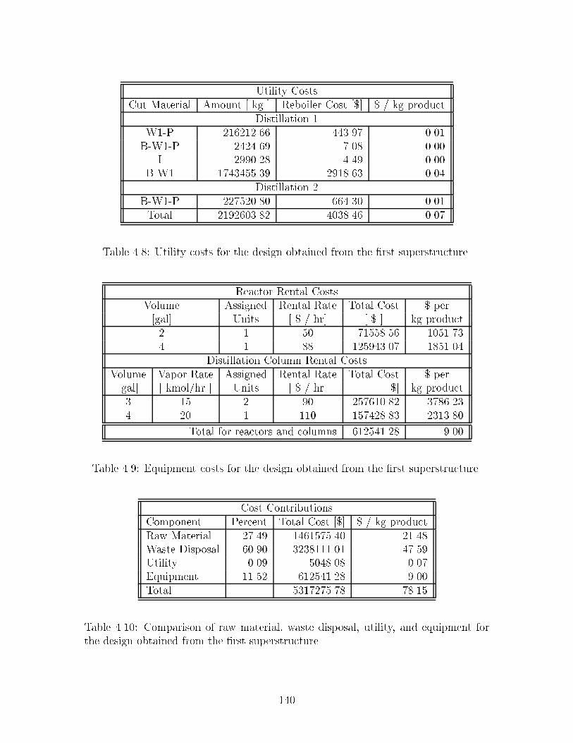
Utility CostsCut Material Amount & kg ' Reboiler Cost &�' � � kg product
Distillation �W�P �������� ����� ���
BW�P ������ ��� ���I ������ ��� ���
BW� ��������� ������ ���Distillation �
BW�P �������� ����� ���Total ��������� ������ ���
Table ��� Utility costs for the design obtained from the �rst superstructure
Reactor Rental CostsVolume Assigned Rental Rate Total Cost � per&gal' Units & � � hr' & � ' kg product� � �� ������� ������� � �� �������� ������
Distillation Column Rental CostsVolume Vapor Rate Assigned Rental Rate Total Cost � per&gal' & kmol�hr ' Units & � � hr' &�' kg product� �� � �� �������� ������� �� � ��� �������� ������
Total for reactors and columns �������� ���
Table ��� Equipment costs for the design obtained from the �rst superstructure
Cost ContributionsComponent Percent Total Cost &�' � � kg productRaw Material ���� ��������� ����Waste Disposal ���� ��������� ����Utility ��� ������ ���Equipment ���� �������� ���Total ��������� ����
Table ���� Comparison of raw material� waste disposal� utility� and equipment forthe design obtained from the �rst superstructure
���
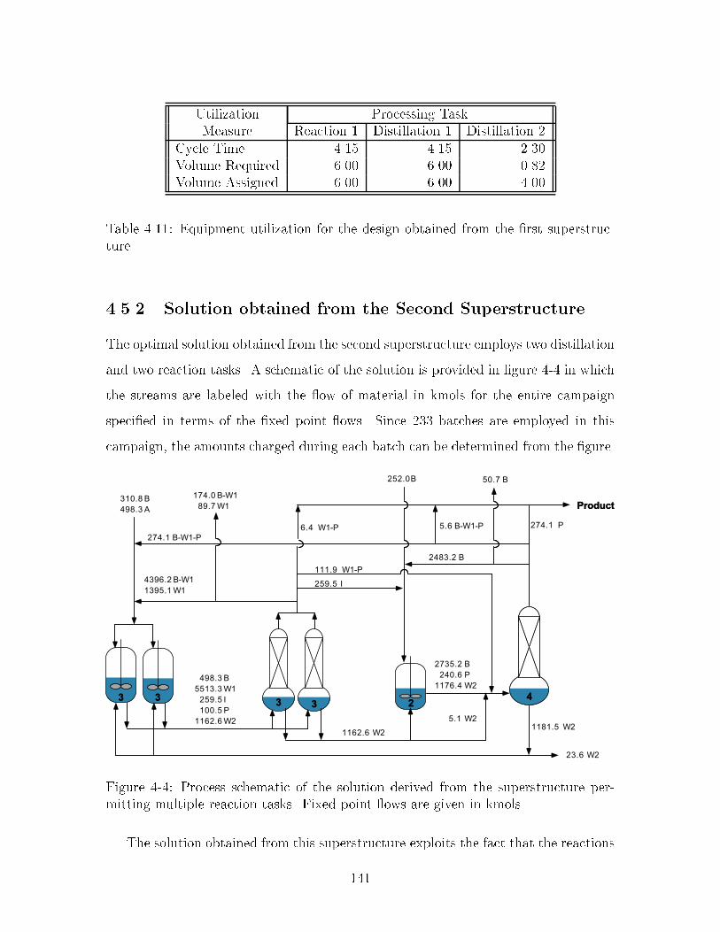
Utilization Processing TaskMeasure Reaction � Distillation � Distillation �
Cycle Time ��� ��� ���Volume Required ��� ��� ���Volume Assigned ��� ��� ���
Table ���� Equipment utilization for the design obtained from the �rst superstructure
���� Solution obtained from the Second Superstructure
The optimal solution obtained from the second superstructure employs two distillation
and two reaction tasks A schematic of the solution is provided in �gure �� in which
the streams are labeled with the ow of material in kmols for the entire campaign
speci�ed in terms of the �xed point ows Since ��� batches are employed in this
campaign� the amounts charged during each batch can be determined from the �gure
'
)*
�
#
),
/02+.
--*.+.
,-0+-
*33+-
**1,+1
'()*
)*
*4/+3
20+4
�,-0+-
)*(#***+0
'()*
)*
/.01+,
*.0-+*
'
#
),
,4.-+,
,/3+1
**41+/
),**1,+1
),,.+1
),**2*+-),-+*
',/2.+,
'()*(#,4/+*
#,4/+*'()*(#-+1)*(#1+/
'-3+4
'
�
.*3+2
/02+.
',-,+3
������ ������
.. .... .. ,,
--
Figure ��� Process schematic of the solution derived from the superstructure permitting multiple reaction tasks Fixed point ows are given in kmols
The solution obtained from this superstructure exploits the fact that the reactions
���
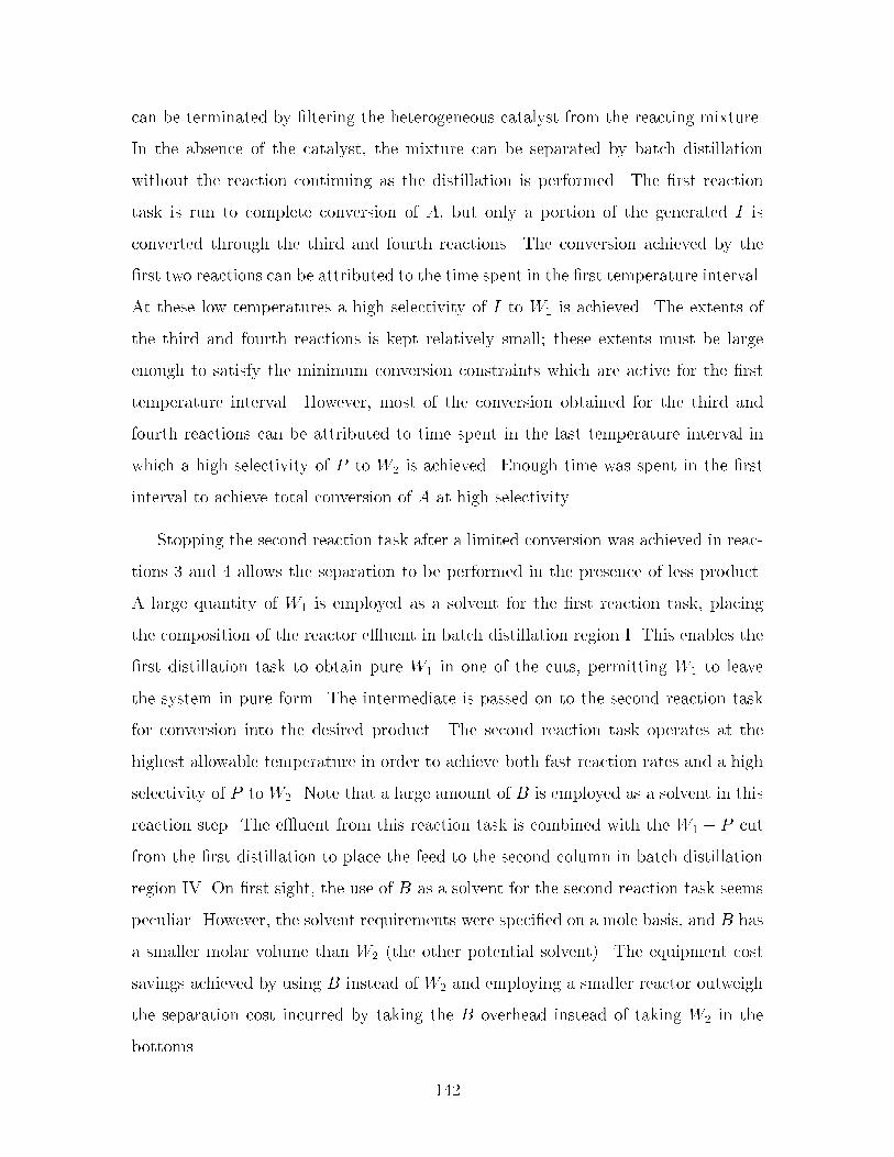
can be terminated by �ltering the heterogeneous catalyst from the reacting mixture
In the absence of the catalyst� the mixture can be separated by batch distillation
without the reaction continuing as the distillation is performed The �rst reaction
task is run to complete conversion of A� but only a portion of the generated I is
converted through the third and fourth reactions The conversion achieved by the
�rst two reactions can be attributed to the time spent in the �rst temperature interval
At these low temperatures a high selectivity of I to W� is achieved The extents of
the third and fourth reactions is kept relatively small� these extents must be large
enough to satisfy the minimum conversion constraints which are active for the �rst
temperature interval However� most of the conversion obtained for the third and
fourth reactions can be attributed to time spent in the last temperature interval in
which a high selectivity of P to W� is achieved Enough time was spent in the �rst
interval to achieve total conversion of A at high selectivity
Stopping the second reaction task after a limited conversion was achieved in reac
tions � and � allows the separation to be performed in the presence of less product
A large quantity of W� is employed as a solvent for the �rst reaction task� placing
the composition of the reactor e)uent in batch distillation region I This enables the
�rst distillation task to obtain pure W� in one of the cuts� permitting W� to leave
the system in pure form The intermediate is passed on to the second reaction task
for conversion into the desired product The second reaction task operates at the
highest allowable temperature in order to achieve both fast reaction rates and a high
selectivity of P to W� Note that a large amount of B is employed as a solvent in this
reaction step The e)uent from this reaction task is combined with the W� � P cut
from the �rst distillation to place the feed to the second column in batch distillation
region IV On �rst sight� the use of B as a solvent for the second reaction task seems
peculiar However� the solvent requirements were speci�ed on a mole basis� and B has
a smaller molar volume than W� �the other potential solvent� The equipment cost
savings achieved by using B instead of W� and employing a smaller reactor outweigh
the separation cost incurred by taking the B overhead instead of taking W� in the
bottoms
���

This design makes fairly e�cient use of both the raw materials and the available
equipment The only way that reactants and products leave the process as waste is
through the purge of recycled streams A more detailed summary of the material
processing costs is provided by tables ���� ���� and ��� The equipment items
are all running at or near capacity� except for the column assigned to the second
distillation task Table ��� shows the charges incurred for the use of equipment
during the campaign� and table ��� shows the utilization of the equipment items
Raw Material CostsRaw Material Cost &� � kg' Feed &kg' Total Cost &�' � � kg product
B ��� ������� �������� ���A ��� ������� �������� ���
Total �������� �������� ����
Table ���� Raw material costs for the design obtained from the second superstructure
Waste Disposal CostsWaste Material Cost &� � kg' Amount &kg' Total Cost &�' � � kg product
B ���� ������ ������� ���W� ���� ������� �������� ����
BW� ���� ������ ������� ���W� ���� ������ �������� ���Total ������� �������� ����
Table ���� Waste disposal costs for the design obtained from the second superstructure
���

Utility CostsCut Material Amount & kg ' Reboiler Cost &�' � � kg product
Distillation �W�P ������� ���� ���W� ��������� ������ ���I ������� ���� ���
BW� �������� ����� ���Distillation �
B �������� ����� ���BW�P ������� ���� ���
P ������� ����� ���Total ��������� ������ ���
Table ���� Utility costs for the design obtained from the second superstructure
Reactor Rental CostsVolume Assigned Rental Rate Total Cost � per&gal' Units & � � hr' & � ' kg product� � �� ������� ������ � �� �������� ������
Distillation Column Rental CostsVolume Vapor Rate Assigned Rental Rate Total Cost � per&gal' & kmol�hr ' Units & � � hr' &�' kg product� �� � �� �������� ������� �� � ��� ������� ������
Total for reactors and columns �������� ���
Table ���� Equipment costs for the design obtained from the second superstructure
Utilization Processing TaskMeasure Reaction � Distillation � Reaction � Distillation �
Cycle Time ��� ��� ��� ���Volume Required ��� ��� ��� ���Volume Assigned ��� ��� ��� ���
Table ���� Equipment utilization for the design obtained from the second superstructure
���

Cost ContributionsComponent Percent Total Cost &�' � � kg productRaw Material ���� �������� ����Waste Disposal ���� �������� ����Utility ��� ������ ���Equipment ���� �������� ���Total ��������� ����
Table ���� Comparison of raw material� waste disposal� utility� and equipment costsobtained for the second superstructure
���� Solution Comparison
The solution obtained from the second superstructure produces a much more e�
cient design This is primarily due to the fact that the waste material W� formed
during the reactions can be removed in pure form in the second case� but not in
the �rst This results in much lower raw material and waste costs The di�erence
in the equipment costs result from the fact that the �rst superstructure requires a
much longer campaign� since it obtains much less product for each batch that is pro
cessed A comparison of the cost contributions between the two campaigns is given
in table ���
Cost First Superstructure Second SuperstructureComponent &� � kg Product' &� � kg Product'
Raw Material ���� ����Waste Disposal ���� ����Utility ��� ���Equipment ��� ���Total ���� ����
Table ���� Comparison of the manufacturing costs of the solutions obtained fromthe two superstructures examined
���

�� Computational Considerations
The screening models presented in this chapter are formulated as mixedinteger linear
programs Although the global optimum of such models can be found using standard
algorithms� the solution time may be prohibitive For these types of problems� strong
formulations are required in order to attempt to solve large problems In addition�
the ability of the linear programming and branch and bound algorithms to solve
these models reliably requires that the model is wellscaled Although the focus of
this research has not been to derive the strongest equivalent formulations for these
models� the procedure used to solve these models can dictate whether solution is
possible in a reasonable time using standard MILP solution codes In this section the
techniques that have been employed to permit the solution of the screening model
are discussed Speci�cally� the modi�cations required to provide a wellscaled model�
the procedure employed to reduce the size of the MILP and obtain tighter bounds
on the continuous variables involved in bilinear terms� and the linearization method
employed for the bilinear terms are described
����� Size of the Models solved
The screening models solved within this thesis are fairly large� and can be di�cult to
solve The following sections cover some of the techniques that have been employed
to solve these models in a reasonable amount of time Table ��� provides statistics
about the size of the models involved in the case studies presented in chapters � and �
Note that the number of binary variables reported treats each SOS� set as one binary
variable� this means that an SOS� set comprised of �ve binary variables �eg� the
variable yFAl in chapter �� is counted as only one binary variable rather than �ve For
reference� the number of SOS� sets has been included in the table The solution times
reported for the models are given to provide a rough idea of how long the models take
to solve� The solution times depend on what type of machine on which the models
�The case study from chapter � containing only one reaction task contains more variables andconstraints than the superstructure containing two reaction tasks because more batches were permit�
���

Case Binary SOS� Continuous of ApproximateStudy Variables Sets Variables Constraints Solution Time
Chapter � One Rxn �� � � � ��� ��� hrs
Chapter � Two Rxns �� � � �� ���� ��� hrs
Chapter � Case I�A �� �� ���� ��� ��� hrs
Chapter � Case I�B �� �� ���� ���� �� min
Chapter � Case II �� �� �� � ���� �� min
Chapter � Case III �� �� ��� �� � �� min
Table ���� Size and approximate solution times for the screening models solved inchapters � and � on an HP J��� workstation
were solved and what other jobs were running on the machine All the models were
solved using OSL �IBM� ����� within GAMS �Brooke et al�� �����
����� Scaling of the Linear Programs
The model described in the preceding sections can lead to linear programs that are
su�ciently poorly scaled to cause the simplex codes to fail due to numerical problems�
such problems were encountered within both OSL �IBM� ����� and CPLEX �CPL�
����� The poorly scaled LPs are the result of nonzero elements of the constraint
matrix that vary over many orders of magnitude In many situations� such problems
result from a poor choice of units for the modeling variables �analogous to the col
umn�variable scaling discussed in chapter �� However� poorly scaled models can also
be the result of modeling decisions such as whether certain tradeo�s are important
or not
The scaling problems within these models come from the linearized constraints
employed to bound the conversion of reactants with respect to time and temperature
such as those appearing in ����� and ����� When the terms e��Tj�tjm become very
small� these constraints are very poorly scaled because the coe�cient for the extents
are unity� but the coe�cient of time is a nonzero value that is approaching zero
with larger values of %tjm In order to avoid these scaling problems� a di�erent time
ted in the one reaction case� The number of batches is represented by an SOS� set that is involvedin bilinear terms� so the number of variables and equations is larger�
���

discretization was selected for reactions � and � and reactions � and � in each time
interval The times were selected to correspond to conversions that were di�erent from
unity by at least the optimization tolerances If we had selected only one time grid�
then we could ignore these constraints for values of e��Tjtm below some threshold
This threshold value indicates the point in time at which the slope of � � e��Tjt
is small enough to be ignored Eliminating these constraints makes the model well
scaled However� the elimination of these constraints de�nes a threshold time beyond
which total conversion can be achieved� whereas in reality total conversion is never
achieved We have found that both approaches lead to a well scaled model� but have
chosen to employ di�erent time discretization for each temperature interval in the
examples considered in this chapter
����� Solution Procedure
A sequence of simpler models is solved before the full screening model is solved These
simpler models are solved for three main reasons� �� to obtain tighter bounds on the
continuous variables that are involved in the bilinear expressions appearing in the
model� and �� to reduce the size of the MILP that is attempted� and �� to determine
a feasible assignment of a large number of the integer decision variables� permitting
an incumbent solution to be found with little additional e�ort
In the sequence of models that is solved� the number of integer variables appearing
in the model is increased By solving the simpler models �rst� a feasible value of the
integer variables for the larger problem can be determined with little additional e�ort
For example� �rst the cost of raw material and waste disposal costs is minimized using
simple bounds for the reaction selectivity that assume only one temperature interval
and no bounds on the extents of reaction versus time The location of the bottoms
cut is not de�ned and processing times are not considered In this model� the only
binary variables that appear are those de�ning the active batch distillation region
and those identifying whether the reaction tasks are performed This model can be
solved quickly The binary variables from the optimal solution are then �xed� and a
more complicated model that includes the de�nition of the bottoms is then solved for
���

the same objective function The solution to this problem provides what is hoped to
be a good solution� but probably not optimal All of the integer variables are then
set free� and the problem is solved again However� the solution just obtained for this
model is provided to the optimizer and is used to prune the branch and bound tree
All branches with solutions worse than this value �the incumbent� are not examined
The incumbent value could also be determined using heuristic methods In fact� good
heuristic methods may provide better incumbent solutions However� as we discuss in
the next paragraph� some of the simple models must be solved to global optimality�
since we employ their solution to provide rigorous bounds on parameters appearing
in the model
Another reason for solving the simple models is to provide tighter bounds on
parameters appearing in the screening model that are used to linearize the bilinear
expressions� or to reduce the size of the screening model For instance� the mini
mum campaign length is used in the linear expressions de�ning the time that each
equipment item is employed While we have found that solving for the minimum
campaign length is more di�cult than solving the screening model� we can obtain
a lower bound on the minimum campaign length by solving two simpler problems
We determine both the minimum number of batches that is required to meet the
production demands and a lower bound on the processing time for the distillation
tasks If we ignore the equipment allocation constraints� a lower bound on the min
imum distillation processing time can be determined from the amount of material
taken overhead in the distillation columns This bound may not be very tight since
the same distillation columns can be used for all of the distillations� yet it tightens
the linearization of the bilinear terms� improving the e�ciency of the branch and
bound procedure Similarly� determining the minimum number of batches serves two
purposes� it de�nes a lower bound for the campaign length when used in conjunction
with the lower bound on the distillation processing time� and it allows the size of the
MILP to be reduced The number of batches is represented using an SOS� set� ie�
N batch �P
nb yNBnb Some of the constraints that are generated result from linearizing
bilinear terms involving yNB These constraints are only generated for values of nb
���

that are greater than or equal to the minimum number of batches� for values of nb that
are less than the minimum� any feasible solution has yNBnb � �� and the corresponding
constraints are inactive Therefore� these constraints can be safely eliminated
The sequence of models that is solved is listed below� with a short description of
the reason for solving each model
Material� This model determines a lower bound on the raw material and waste
disposal cost for the manufacturing campaign Simple bounds on the selectivity
are imposed No dependence on time is considered The solution provides a
lower bound on the raw material and waste costs and identi�es the active batch
distillation regions
Bottoms� This model identi�es the location of the bottoms cuts and minimizes the
raw material� utility� and waste disposal costs The targets for the extents
of reaction described in this chapter are employed The utility cost that is
calculated represents a lower bound on the utility cost determined by the full
screening model� because the minimum re ux ratio of all of the columns that
are available is employed to calculate the utility costs
Distillation Time This model determines a lower bound on the total processing
time required for the distillation tasks The model is �rst solved with the binary
variables �xed at the solution of the Bottoms model to provide an incumbent
solution The model is then solved to optimality with all of the binary variables
remaining free
Batches The minimum number of batches is determined This model determines a
feasible allocation of the equipment units that minimizes the number of batches
required First� the model is solved with the location of the distillation cuts
held �xed� providing an upper bound on the optimal solution Next� a relaxed
model is solved The solutions of these two models provide upper and lower
bounds on the minimum number of batches and are used to reduce the size of
the Batches model Finally� the model is solved to optimality The optimal
���

solution of Batches is used to reduce the size of the screening model Note that
the fact that the number of batches is an integer value can be exploited when
determining the termination criteria of the branch and bound algorithm The
solution also provides a lower bound on the campaign cost when combined with
the solution of the Distillation Time model
Units The minimum number of equipment units required to manufacture the product
is determined This quantity has been employed to tighten the constraints
de�ning the time that the equipment units are used which result from the exact
linearization of the bilinear expressions involving the campaign length and the
SOS� variables denoting how many equipment items of a particular type are
employed �see section ����
Screening Model This model minimizes the equipment� utility� raw material� and
waste disposal costs The values of the integer values determined from the
solution of Units and Batches can be employed to quickly solve the Screening
Model to obtain an upper bound on the solution The smallest of these can
be employed as an incumbent Heuristics can also be employed to de�ne an
incumbent solution� but this has not been investigated in any detail However�
the screening model can be solved quickly when the allocation of the equipment
items is �xed� so this could be exploited in deriving a heuristic procedure to
specify the incumbent
����� Linearization of Bilinear Terms
The screening model that has been presented has been written in a form that con
tains only binary and continuous variables The integer variables in the model have
been replaced by binary variables� for example� NB �PN
n�� yNn n However� the
model originally contained bilinear expressions that have been eliminated through
the introduction of additional continuous variables and constraints to cast the model
as a MILP Since all of the bilinear terms in the original model are between two
binary variables or between a binary and a continuous variable� an exact transfor
���

mation exists and has been employed Although several ways in which to generate
linear constraints de�ning an equivalent convex hull of integral solutions exist� the
choice of the linearization technique can have a major impact on the strength of the
formulation �the way in which the relaxed problem approximates the convex hull�
We have applied ideas developed in the operations research community to carry out
this transformation in a systematic fashion� employing the method leading to the
strongest formulation whenever the choice between the methods was clear We have
not considered algorithms designed to deal directly with the bilinear models �Quesada
and Grossmann� ����� AlKhayyal� ����� although we recognize that research in this
area may enable these models to be solved more e�ciently We have employed the
techniques of Glover ������ ����� and Adams and Sherali �Adams and Sherali� �����
Adams and Sherali� ����� Adams and Sherali� ����� to transform the original bilinear
expressions into linear inequalities
First� we show the way that the bilinear terms in the model can be replaced with
new continuous variables that equal the original bilinear expression for all integer val
ues of the binary variables The screening model contains bilinear terms between two
binary variables� or between a binary and a continuous variable An exact lineariza
tion for each type of expression was proposed by Glover ������ Let x � &xLO� xUP '
and y�� y� � f�� �g represent the continuous and binary variables involved in the bilin
ear terms xy� and y�y� Continuous variables zC � xy� and zB � y�y� are introduced
to replace these terms The following inequalities �Glover� ����� de�ne zC �
x� xUP ��� y�� � zC � x� xLO��� y�� �����
xLOy� � zC � xUPy� �����
and the following inequalities de�ne zB �Glover and Wolsey� ������
zB � y� �����
zB � y� �����
zB � y� " y� � � �����
���

However� ��������� only de�ne zC and zB exactly when y� and y� take integer
values Since the binary variables are relaxed during the solution of the MILP� how
well these constraints approximate the convex hull is important The values chosen
for xLO and xUP have a major impact on the way in which ��������� a�ect the
integrality gap of the problem A poor choice of xLO and xUP will lead to a loose
LP relaxation These models may be solved more e�ciently if tight bounds on the
continuous variables involved in the bilinear expressions can be derived The solution
procedure that we have proposed attempts to derive tight bounds for these quantities�
but we recognize that these constraints have a negative impact on the performance
of the solution algorithms
The work of Adams and Sherali ������ ����� ����� addresses the strength of
the formulation resulting from the exact linearization of bilinear terms involving bi
nary variables They address mixedinteger zeroone quadratic programming prob
lem �MIQPP� and mixed integer bilinear programming problems �MIBLP� MIQPP
and MIBLP problems can be reformulated using one of several exact linearization
methods �Adams and Sherali� ����� Adams and Sherali� ����� The di�erent lin
earization schemes a�ect the number of constraints in the resulting mixed integer
zeroone linear program and the tightness of the linear programming relaxation The
linearization technique proposed by Adams and Sherali ������ has been shown to the
oretically dominate previously proposed linearization techniques �Glover and Wolsey�
����� Glover� ����� for MIQPP problems However� this technique results in a larger
number of constraints They also propose an e�cient solution algorithm for the MI
BLP problems �Adams and Sherali� �����
Their technique generates a tight linear reformulation for mixedinteger zeroone
programming problems The original constraints in the problem are multiplied by
every binary variable to derive an additional set of nonlinear constraints The con
straints involving only binary variables are multiplied by the di�erences between the
continuous variables and their bounds �eg� xUP � x and x� xLO� Continuous vari
ables are then introduced to represent the bilinear terms using the same linearization
�Sometimes constraints in this form are referred to as �Big M� constraints�
���

scheme proposed by Glover ������� resulting in a mixedinteger linear model
Unfortunately� the screening model developed in the preceding chapter is not in
MIQPP or MIBLP form� MIQPP and MIBLP models require that all of the bilinear
terms in the model appear in the objective function All of the bilinear terms de�ning
costs� ���������� can be moved into objective function� but the remaining bilinear
terms in the screening model cannot be directly moved to the objective function
Noting that the techniques developed by Adams and Sherali lead to a tighter for
mulation� but do not apply directly to our problem� we have applied their ideas in the
following fashion First� we employ the exact linearization proposed by Glover ������
to generate an exact linearization of all of the bilinear terms originally appearing in
our model Next� we apply the basic idea proposed by Adams and Sherali ������
����� in a limited sense We look at the set of new continuous variables that we have
introduced and multiply any equations containing only binary variables by the di�er
ence between the continuous variables and their bounds or by other binary variables
if these multiplications will not introduce any additional continuous variables We
multiply the other constraints by any binary variables that will not introduce any
additional continuous variables due to new bilinear terms This idea was carried out
manually� so new equations that could have been introduced may have been missed
The application of the idea presented above seems to have the biggest impact when
the SOS� variables were involved in bilinear expressions For example� consider the
bilinear term ynf � fn whereP
n yn � � and f � &�� fUP ' The application of the
procedure results inP
n�ynfUP � fn� � fUP � f which reduces to
Pn fn � f Al
though these constraints are somewhat obvious from a physical understanding of the
system� they are derived by this procedure Although other constraints were derived
and added to the model� the biggest impact on the e�ciency seemed to come from
the constraints involving the SOS� variables
To compare the bene�ts of the di�erent linearization strategies e�ectively� the
transformations from the bilinear model to the di�erent equivalent linear representa
tions must be performed automatically This was not attempted because the proposed
models could be solved with the strategy that was applied However� if the solution
���
of much larger models is attempted� automatic derivation of a tighter equivalent lin
ear model may be required With di�erent strategies implemented automatically� the
tradeo� between model size and solution e�ciency can be investigated empirically
���� In uencing the Branch and Bound Algorithm
Features of the models have been exploited to improve the performance of the branch
and bound procedure These include the identi�cation of SOS� sets and the use of
variable priorities
Many of the binary variables in the system represent special ordered sets of type
� �SOS�� �Beale and Tomlin� ������ such as the number of batches and the type of
distillation column assigned to a distillation task Declaring these variables as SOS�
sets allows the branch and bound algorithm to employ a di�erent branching procedure
for these sets Typically� during the branching procedure� the variables in the set are
divided into subsets in which one subset contains the nonzero element and the other
does not This di�ers from the usual practice of �xing a binary variable to either
zero or one along each branch� and is much more e�cient when the SOS� sets contain
many elements For small sets� the bene�ts may not be very pronounced In addition�
the fact that these variables must sum to one helps when linearizing the bilinear terms
between the SOS� and continuous variables This is explained in section ���
Since some of the decisions in the design of the process are naturally made in a
sequential fashion� this sequence can be used to indicate a preferred branching order
for the branch and bound algorithm For instance� there is no point in deciding which
distillation column to assign to a separation task if the separation is not performed
The same holds for the reaction tasks Variable priorities are a way to represent the
preferred branching order to the solvers embedded within GAMS �Brooke et al�� �����
Empirical evidence has also suggested the addition of an SOS� set to represent the
number of items of a particular equipment item assigned to the process When this set
is employed in conjunction with the setting of priorities� the branch and bound decides
whether to employ a particular item of equipment before determining where to assign
the unit Experience solving these models has shown that the following ordering of
���

the discrete decisions �from top to bottom in the tree� improves the performance of
the algorithm�
� the existence of the reaction tasks
� the existence of the distillation tasks
� the identity of the active batch regions
� the number of distillation columns assigned to a particular separation
� the location of the bottoms cuts
� what equipment units are employed within the process
� the allocation of reactors and columns to particular tasks
� identifying the active feed and time intervals
� determining the number of batches
����� Tailored Solution Procedures
This research has not investigate tailored solution procedures for the solution of the
screening models However� it is easy to recognize that a tailored solution procedure
would be more e�ective on the screening models� particularly one that can exploit
the way in which the number of batches has been modeled For the models with no
intermediate storage� all units employ the same number of batches� so the number
of batches has been represented using a single SOS� set The size of this set a�ects
the number of equations in the model to be solved In addition� the upper and lower
bounds on the number of batches appear in the constraints used to linearize the
bilinear expressions involving the number of batches and any continuous variables
�eg� terms de�ning the charge of material to a particular task for each batch� Thus�
by restricting the number of batches to several smaller ranges� not only can the
size of the model in each range be reduced� but each of these models will result in
a tighter formulation since the tighter upper and lower bounds can be employed
���

A tailored branch and bound procedure could reduce the size of the models and
update the parameters when branching on members of the SOS� set Although the
implementation of such a procedure is a nontrivial task� it may be required to handle
situations employing unlimited intermediate storage� or cases in which intermediate
storage is employed to decouple only some of the processing trains In these situations�
the screening model includes a number of batches for each processing step
����� Representation of Batch Distillation Boundaries
The boundaries of each of the product simplices are included in the each of the batch
distillation regions Thus� if the feed to a distillation column is located on a boundary�
two choices of the binary variables lead to exactly the same solution This requires
the branch and bound procedure to search each of the trees to verify the solution
These situations are common and will almost always arise from the addition of an
entrainer For instance� in the solution to the superstructure containing only one
reaction task� both distillation tasks have feeds located on the boundary located
between two distillation regions Future work should investigate ways to avoid this
type of problem
��� Summary
The application of the screening models to a fairly simple process has been examined
This chapter demonstrates how the design constraints and the restrictions imposed
by the manufacturing facility can be used to derive bounds for the extent of reac
tion versus time and for the selectivity of competing reactions However� even for a
reasonably simple problem� the derivation of these bounds may be a nontrivial task
The application of the bounds to two di�erent superstructures demonstrates that
even rough approximations of the reaction behavior can capture many of the tradeo�s
that need to be considered at the design stage In fact� solution of the screening
model may exploit tradeo�s that are not obvious to the engineer In some cases� these
solutions may indicate that the screening model should be augmented with additional
���

constraints to capture some particular physical behavior that was relaxed during the
derivation of the screening model For example� the solution chose not to perform
any of the third and fourth reactions in the one of the reactors until a constraint
requiring a minimum conversion with respect to the reaction time was added In other
cases� the solution of the screening model may generate design alternatives that di�er
substantially from the designs produced through minor modi�cations of the chemists
recipe In retrospect� the solution determined from the second superstructure seems
obvious However� if we had started with the mindset of adapting the chemists design
to account for the fact that we could not operate at such a low temperature� we may
have ended up with a design looking much more like the one obtained from the �rst
superstructure
The di�erence in the solution obtained from the two superstructures demonstrates
the need to consider a broad range of alternatives early in the design of the process
This highlights both a strength and a weakness of the screening models in the ex
ample presented First� by only including a subset of the constraints the models do
not eliminate any promising designs contained within the superstructure However�
since only reaction�distillation processes are included within the current superstruc
ture� many batch processes of interest cannot be described by the screening models
described here Thus� targeting models for other common processing tasks such as
extraction� crystallization� etc should be investigated in the future
�� Notation
The notation that has been introduced in this chapter is de�ned in the lists below
����� Indexed Sets
J The set de�ning the temperature intervals For j � J � Tj�� and Tj represent
the lower and upper bounds of the interval
���
L The set de�ning the feed intervals For l � L� %fl�� and %fl represent the lower
and upper bounds of the interval
M The set de�ning the time intervals For m � M � tm�� and tm represent the
lower and upper bounds of the interval Note that t� � �
����� Binary Variables
yFAl SOS� set denoting the active feed interval for the A charged
yFIl SOS� set denoting the active feed interval for the I charged and the I gen
erated by reaction �
ytjm SOS� set denoting the active time interval in temperature interval j
����� Variables
NAjm the amount of A available for reaction in the time interval m and tempera
ture interval j NAjm � ytjmf
RinA
�t�jm Continuous variable representing a bilinear product between the following
continuous and binary variables �t�jm � ytjm�T�j
�Trj the extent of reaction r attributed to temperature interval j
(�Trjl the extent of reaction r attributed to temperature interval j and feed interval
l NoteP
l(�Trjl � �Trj
x��j the fractional conversion of A achieved in reactions � and � in temperature
interval j
x��j the fractional conversion of I achieved in reactions � and � in temperature
interval j
x��S
j the fractional conversion of A achieved in reactions � and � in temperature
intervals � to j
x��S
j the fractional conversion of I achieved in reactions � and � in temperature
intervals � to j
����� Parameters
%fAl upper bound on fRinA in feed interval l
���

%f Il upper bound on feed of I �fRinI " ��� in feed interval l
%tjm time discretization point m for temperature interval j
Tj Upper bound on temperature in temperature interval j
%x�max
jm Maximum fractional conversion achieved in reaction � in temperature in
terval j and time interval m
%x��min
jm Minimum fractional conversion achieved in reactions � and � in temperature
interval j and time interval m
���

Chapter �
Siloxane Monomer Case Study
In this chapter screening models are applied to the design of a process for the campaign
manufacture of siloxane monomer �Barrera� ����� Allgor et al�� ����� This example
is an abstraction of a problem actually encountered by a major specialty chemical
manufacturer The identities of the compounds involved have been concealed
The scenario is as follows Research chemists have recently discovered a new
siloxane based polymer� and a signi�cant quantity is now required for test marketing
This example focuses on the development of a campaign to manufacture a �xed
quantity of the monomer Since the development of similar products by competitors
is imminent� both the process development activity and the resulting campaign are
subject to a strict time horizon constraint It is also likely that the design will be
used to estimate the cost of long term manufacture Hence� rapid development of an
e�cient process is pivotal to the success of the new product The goal of the screening
model is to identify favorable process structures quickly� so that these may serve as
the starting point for the detailed design
The process consists of three reaction tasks that manufacture two products� prod
uct A is generated in the �rst reaction and product D is generated in the third Two
applications for the mixedinteger linear screening models are considered First� the
solution from the screening models is compared to that obtained when minimizing
the waste generated by the process �Ahmad and Barton� ����� to examine whether a
process generating the minimum amount of waste can make e�cient use of equipment
���
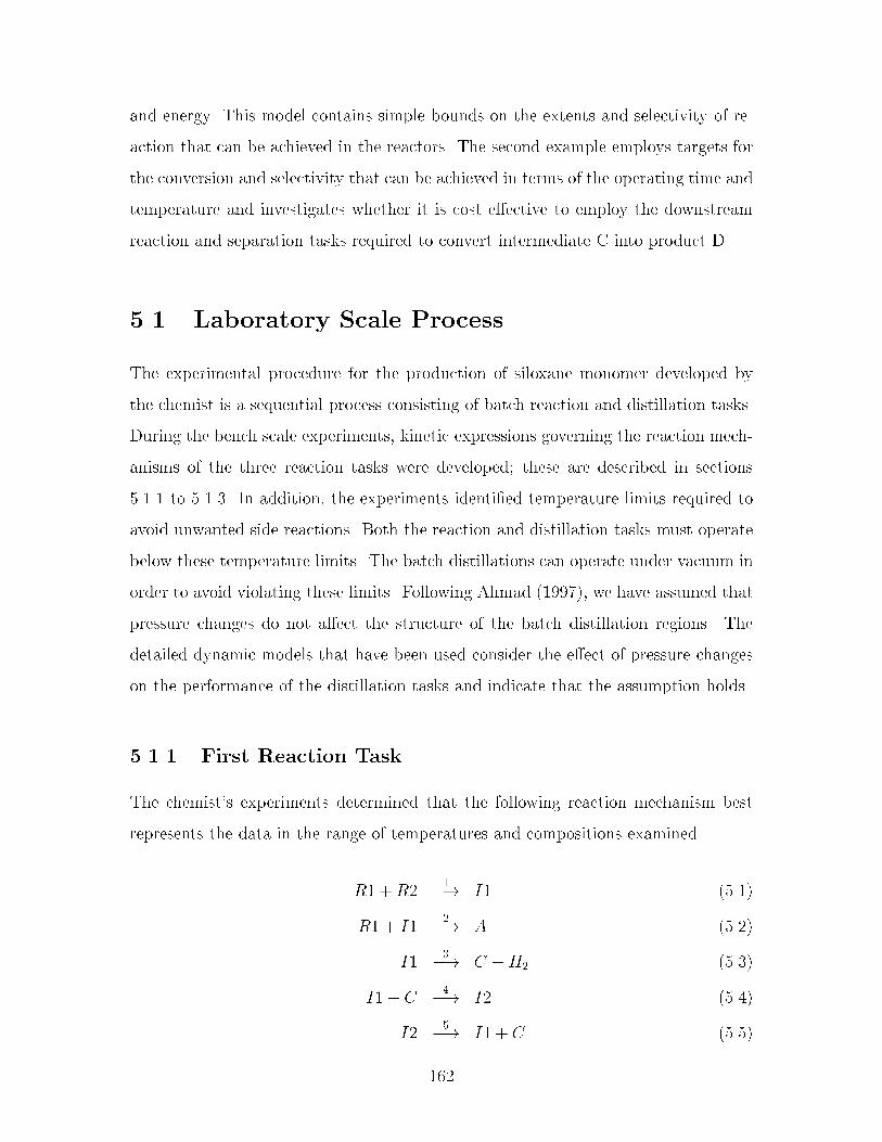
and energy This model contains simple bounds on the extents and selectivity of re
action that can be achieved in the reactors The second example employs targets for
the conversion and selectivity that can be achieved in terms of the operating time and
temperature and investigates whether it is cost e�ective to employ the downstream
reaction and separation tasks required to convert intermediate C into product D
�� Laboratory Scale Process
The experimental procedure for the production of siloxane monomer developed by
the chemist is a sequential process consisting of batch reaction and distillation tasks
During the bench scale experiments� kinetic expressions governing the reaction mech
anisms of the three reaction tasks were developed� these are described in sections
��� to ��� In addition� the experiments identi�ed temperature limits required to
avoid unwanted side reactions Both the reaction and distillation tasks must operate
below these temperature limits The batch distillations can operate under vacuum in
order to avoid violating these limits Following Ahmad ������� we have assumed that
pressure changes do not a�ect the structure of the batch distillation regions The
detailed dynamic models that have been used consider the e�ect of pressure changes
on the performance of the distillation tasks and indicate that the assumption holds
���� First Reaction Task
The chemist�s experiments determined that the following reaction mechanism best
represents the data in the range of temperatures and compositions examined
R� "R��� I� ����
R� " I��� A ����
I��� C "H� ����
I� " C�� I� ����
I��� I� " C ����
���

Pt � Pt� ����
Note that the �rst reaction is catalyzed by the platinum catalyst �Pt�� the cata
lyst can deactivate to Pt� over the course of the reaction The chemists discovered
that unwanted side reactions are catalyzed at temperatures above ��� K� therefore�
such temperatures must be avoided Further analysis determined that the following
expressions best describe the rates of reaction The constants for these equations
are provided in table �� where the units of the preexponential factors �kr�� provide
reaction rates in mols��m�� when the concentrations are measured in molm�
rate� � �CR�CR�CPt
k� " CPt����
rate� � �CR�CI� ����
rate� � �CI� ����
rate� � �CI�CC �����
rate� � �CI� �����
rate � CPt �����
where the temperature dependence of the rate constants are given by the following
Arrhenius expression�
r � r�ef�EaRT g � r � ����
���� Second Reaction Task
The second reaction task converts the intermediate C generated in the �rst reaction
task to a second intermediate E by reacting C with methanol �M� according to the
following stoichiometric relationship�
M " C � E �����
���

r Ea &Jmol��' r�� ����� ��� x ���
� ����� ���� ������ ��� x ����
� ����� ��� x ����
� ����� ��� x ���
� � ��� x ����
� � ��� x ����
Table ��� Preexponential factors and activation energies de�ning the rate constants�������� for reactions ������� occurring within the �rst reaction task
Equation ����� de�nes the rate of reaction ����� The chemists imposed an up
per temperature limit of �� K on the operating temperature and determined a rate
constant at this temperature of �� m��kmol hr� for concentrations measured in
kmolm�
rate � CCCM �����
���� Third Reaction Task
The third reaction task converts the intermediate E generated in the second reaction
task to product D by reacting E with water W according to the following stoichio
metric relationship�
�E "W � D " �M �����
Equation ����� de�nes the rate of reaction ����� for the stoichiometry written in
�����
rate � CCCM �����
���

The preexponential factor and the activation energy for this reaction are given below�
� � ������ �����
m�
kmol hr
������
Ea � �����
�J
mol
������
The chemists advise that this reaction is run below �� C� and this is treated as a
design constraint
���� Design Constraints
Several design decisions have been made that restrict the operation of the reactors
Total conversion of R� is required in the �rst reaction� a minimum of ��# conversion
of C to E is required in the second reaction� and a minimum of ��# conversion of E
to D is required in the �nal reaction
fRout��R� � � �����
��� ����Xe�E
fRin�e �Te �C � fRout��C �����
��� ����Xe�E
fRin�e �Te �E � fRout��E �����
Restrictions are also placed on the amount of toluene needed to solvate the �rst
reaction In addition� an excess of the nonlimiting reagent is required in each of the
reactions� at least a ��# excess of R�� a three to one ratio of methanol to C� and a
�� to one ratio of water to E are required
Xe�E
fRin�e �Te �T � ���Xe�E
fRin�e �Te �R� �����
fRout��R� � ���Xe�E
fRin�e �Te �R� �����
Xe�E
fRin�e �Te �M � �Xe�E
fRin�e �Te �C �����
Xe�E
fRin�e �Te �W � ��Xe�E
fRin�e �Te �E �����
���

In addition� we require that only toluene� water� methanol� R�� and R� may be
supplied to the process The product must consist of ��# A and D on a mass basis
Letting Xproduct � ���� and EP � fA�Dg� the purity constraint ����� reduces to the
following�
���Xe
fPe �Tew � fPA�
TAw " fPD�
TDw �����
�� Case Study I� Comparison of minimum cost
versus minimum waste
We require the manufacture of ������� kilograms of monomer in less than sixty days
In this problem we compare the di�erence between minimizing the manufacturing
cost and minimizing the manufacturing cost subject to minimum waste emissions
Ahmad ������ has shown that an embedded optimization that �rst minimizes the
waste emitted by the process and then minimizes the total ow of recycled material
while permitting no more than the minimum waste to be emitted leads to sensible
process designs with minimum environmental impact In this section� we compare
the di�erence between minimizing the total cost and minimizing the total cost of a
design that emits no more than the minimum amount of waste
The screening models employed for this case study employ a simpli�ed model
of the �rst reaction task that considers the two dominant reactions given in �����
����� rather than the set of competing reactions ������� The intermediate species
generated in the �rst reaction are not included in the screening model We assume
that hydrogen remains in the gas phase� and that no cost is incurred when sending
the hydrogen to the are
�R� " R��� A �����
R� " R��� C "H� �����
Toluene is not permitted to mix with water in order to avoid the formation of two
���
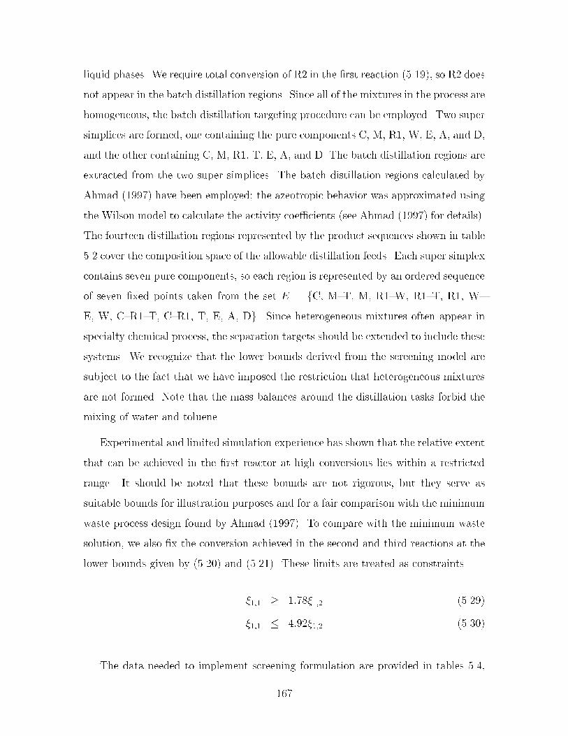
liquid phases We require total conversion of R� in the �rst reaction ������ so R� does
not appear in the batch distillation regions Since all of the mixtures in the process are
homogeneous� the batch distillation targeting procedure can be employed Two super
simplices are formed� one containing the pure components C� M� R�� W� E� A� and D�
and the other containing C� M� R�� T� E� A� and D The batch distillation regions are
extracted from the two super simplices The batch distillation regions calculated by
Ahmad ������ have been employed� the azeotropic behavior was approximated using
the Wilson model to calculate the activity coe�cients �see Ahmad ������ for details�
The fourteen distillation regions represented by the product sequences shown in table
�� cover the composition space of the allowable distillation feeds Each super simplex
contains seven pure components� so each region is represented by an ordered sequence
of seven �xed points taken from the set E � fC� M�T� M� R��W� R��T� R�� W�
E� W� C�R��T� C�R�� T� E� A� Dg Since heterogeneous mixtures often appear in
specialty chemical process� the separation targets should be extended to include these
systems We recognize that the lower bounds derived from the screening model are
subject to the fact that we have imposed the restriction that heterogeneous mixtures
are not formed Note that the mass balances around the distillation tasks forbid the
mixing of water and toluene
Experimental and limited simulation experience has shown that the relative extent
that can be achieved in the �rst reactor at high conversions lies within a restricted
range It should be noted that these bounds are not rigorous� but they serve as
suitable bounds for illustration purposes and for a fair comparison with the minimum
waste process design found by Ahmad ������ To compare with the minimum waste
solution� we also �x the conversion achieved in the second and third reactions at the
lower bounds given by ����� and ����� These limits are treated as constraints
���� � �������� �����
���� � �������� �����
The data needed to implement screening formulation are provided in tables ���
���
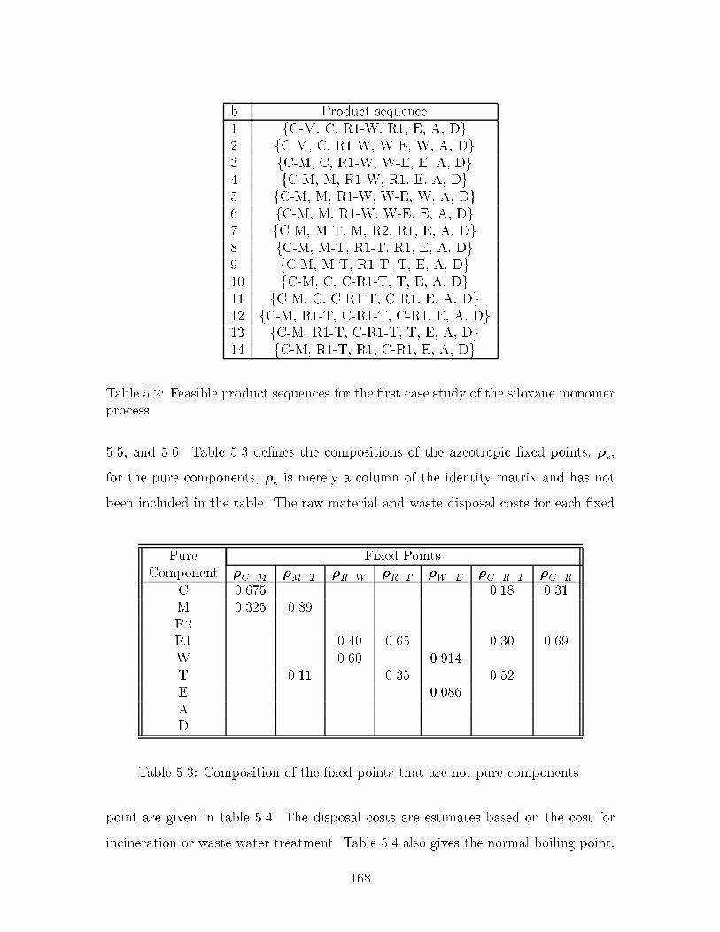
b Product sequence� fCM� C� R�W� R�� E� A� Dg� fCM� C� R�W� WE� W� A� Dg� fCM� C� R�W� WE� E� A� Dg� fCM� M� R�W� R�� E� A� Dg� fCM� M� R�W� WE� W� A� Dg� fCM� M� R�W� WE� E� A� Dg� fCM� MT� M� R�� R�� E� A� Dg� fCM� MT� R�T� R�� E� A� Dg� fCM� MT� R�T� T� E� A� Dg�� fCM� C� CR�T� T� E� A� Dg�� fCM� C� CR�T� CR�� E� A� Dg�� fCM� R�T� CR�T� CR�� E� A� Dg�� fCM� R�T� CR�T� T� E� A� Dg�� fCM� R�T� R�� CR�� E� A� Dg
Table ��� Feasible product sequences for the �rst case study of the siloxane monomerprocess
��� and �� Table �� de�nes the compositions of the azeotropic �xed points� �e�
for the pure components� �e is merely a column of the identity matrix and has not
been included in the table The raw material and waste disposal costs for each �xed
Pure Fixed PointsComponent �C�M �M�T �R�W �R�T �W�E �C�R�T �C�R
C ���� ��� ���M ���� ���R�R� ��� ��� ��� ���W ��� ����T ��� ��� ���E ����AD
Table ��� Composition of the �xed points that are not pure components
point are given in table �� The disposal costs are estimates based on the cost for
incineration or waste water treatment Table �� also gives the normal boiling point�
���

the heat of vaporization� and the molar volume and molecular weight of the �xed
points Note that the molar volume and heat of vaporization are underestimates
for these quantities over the temperature range that the process operates� the molar
volume� molecular weight� and heat of vaporization for the azeotropes represent ideal
mixture values These bounds are chosen so that the ideal mixing rule employed in
the screening model bounds the mixture volume and heat of vaporization calculated
using an activity coe�cient model or equation of state
Raw Waste Molare Material Removal Tb Hvap Volume Molecular
& � � kg ' & � � kg ' &K' &J�mol' & l � kmol ' WeightCM ���� ���� ����� ���� ������C ���� ���� ����� ����� ������
MT ���� ���� ����� ���� �����M ���� ���� ����� ���� �����R� ��� ���� ���� ����� ����� ������
R�W ���� ���� ����� ���� �����R�T ���� ���� ����� ���� �����R� ��� ���� ���� ����� ���� �����WE ���� ���� ����� ���� �����W ��� ��� ���� ����� ���� �����
CR�T ���� ���� ����� ���� �����I� ���� ���� ����� ����� ������
CR� ���� ���� ����� ���� �����T ���� ���� ���� ����� ����� �����E ���� ���� ����� ����� ������A ���� ���� ����� ����� ������I� ���� ���� ����� ����� ������D ���� ���� ����� ����� ������
Table ��� Cost and physical property data for the �xed points
���� Solution
We require the manufacture of ������� pounds of monomer in less than sixty days
The MILP screening formulation was augmented with the additional constraints
��������� and solved using GAMS�OSL �Brooke et al�� ����� IBM� ����� on an
���

ReactorsVolume Available Rental Rate&gal' Units & � � hr'��� � ����� � ������ � ��
Distillation ColumnsVolume Vapor Rate Number of Minimum Available Rental Rate&gal' &kmol�hr' Trays Re ux Ratio Units & � � hr'��� �� � �� � ������ �� � �� � ������� �� � �� � ���
Table ��� Inventory and rental rates for processing equipment
Utility Cost &� � kW yr'hot ���cold ��
Table ��� Utility cost data for the siloxane monomer example
���

HP J��� computer Two cases have been considered In the �rst case� the total
production cost was minimized subject to the model constraints The second case
examines the use of an embedded optimization �Ahmad� ����� In this case� the min
imum amount of waste emitted from a process meeting the production requirements
was determined �rst� Next� the manufacturing cost of a process emitting no more
than this amount of waste was minimized The amount of waste that can be emitted
is treated as a constraint� and the same objective function �eg� the manufacturing
cost� employed in the �rst case is used The solutions of the two cases are compared
Case IA� Minimum Cost Design
The minimum cost design determined by the screening model chooses to perform two
separation tasks and merge the �rst and second reaction tasks into a single equipment
stage The design employs three reactors and three columns and requires �� batches to
complete the campaign This design manufactures the product at a cost of �����kg
Figure �� depicts a schematic of the process showing the allocation of equipment and
the ow of material in kmols for the campaign Tables ������ show the breakdown
of the costs in the process
Raw Material CostsRaw Material Cost &� � kg' Feed &kg' Total Cost &�' � � kg product
M ��� ����� ����� ���R� ��� ������� �������� ���R� ��� ������� �������� ���W ��� ������ ���� ���T ��� ������ ������ ���
Total �������� �������� ���
Table ��� Raw material costs for the entire campaign when minimizing total cost inthe �rst case study
�All waste streams were weighted equally when determining the minimum amount of wasteemitted�
���

������ ������
5,
5*
6
--*+4
*3*.+2
*1+1
-33 4-3
76
56
6
/+.
-+-
*/+,
76
56
6
,*3+/
,12+2
10.+4
�7,+2
�0.+,
-33*,-3 4-3 4-3
)�
)
*21+4
,/-0+-
�/-2+-
�
7
5*
6
�
�
*+0
*0,+3
*42+.
2,4+1
0.+,
/-2+-
�/1+/
)*23.+*
70*+3
7
)
�
�
0,+2
,12.+2
*1+.2
/1+/
)�
)
.+2
.2+/
)**+4+� +�
7*+2
�7+31
Figure ��� Process schematic of the solution derived for Case IA Streams labelsdenote the ow of each �xed point in kmols for the campaign
���

Waste Disposal CostsWaste Material Cost &� � kg' Amount &kg' Total Cost &�' � � kg product
W ��� ����� ����� ���Total ����� ����� ���
Table ��� Waste disposal costs for the entire campaign when minimizing total costin the �rst case study
Utility CostsCut Material Amount & kg ' Reboiler Cost &�' � � kg product
Distillation �CM ����� ��� ���MT ������ ��� ���RT ������� ��� ���T ������� ��� ���E ������� ��� ���
Distillation �M ������ ��� ���WE ������ ��� ���W ������� ��� ���
Total �������� ��� ���
Table ��� Utility costs for the entire campaign when minimizing total cost in the�rst case study
Reactor Rental CostsVolume Assigned Rental Rate Total Cost � per&gal' Units & � � hr' & � ' kg product��� � �� ������� ������ � �� ������� ���
Distillation Column Rental CostsVolume Vapor Rate Assigned Rental Rate Total Cost � per&gal' & kmol�hr ' Units & � � hr' &�' kg product��� �� � �� ������� ������� �� � ��� ������� ���
Total for reactors and columns �������� ���
Table ���� Equipment costs for the entire campaign when minimizing total cost inthe �rst case study
���

Utilization Processing TaskMeasure Rxn � Rxn � Dist � Rxn � Dist �
Cycle Time ��� ��� ��� ��� ���Volume Required ������ ������ ������ ����� �����Volume Assigned ������ ������ ������ ����� ������
Table ���� Equipment utilization for the design obtained when minimizing total costin the �rst case study
Cost ContributionsComponent Percent Total Cost &�' � � kg productRaw Material ���� �������� ���Waste Disposal ��� ����� ���Utility ��� ��� ���Equipment ���� �������� ���Total ��������� ���
Table ���� Comparison of raw material� waste disposal� utility� and equipment costs
Case IB� Minimum Cost subject to Minimum Waste
In this case� a lower bound on the mass of waste emitted by a process meeting
the production requirements was determined by minimizing the following objective
function�
�waste �Xe�E
fWastee we �����
subject to the mass balance constraints in the screening model �ie� ������� ����
���� �������� and ��������� and the design and reaction targeting constraints
presented in this chapter The solution of the resulting MILP determined that at
least ����� kg of waste must be emitted from a process meeting the production
���

requirement� Next� a design with minimum cost that does not emit more than this
much waste was determined by adding the following constraint to the model solved
in Case IA�
Xe�E
fWastee we � �waste �����
Since only ����� kg of waste is emitted by the solution of Case IA� ����� is satis�ed
by the solution of Case IA� and the solution to this problem is the same as the
solution to Case IA For this example� the solution with minimum environmental
impact �measured by the total mass of waste emitted� is the same as the solution
with minimum cost
Next� we examine how the structure of the process de�ned by the solution to
this problem compares to structure of the minimum waste process found by Ahmad
������ In her method� �rst the minimum amount of waste is determined� and then
the total ow of recycled material is minimized subject to the minimum waste con
straint In this method� the �rst minimization is the same as the �rst subproblem
solved in Case IB� except that she minimized the total moles of wasteP
e�E fWastee
rather than the mass The second subproblem that she solves di�ers from the second
problem solved here because the procedure used by Ahmad ������ does not con
sider the equipment costs Instead� she minimizes the total ow of recycled material
We compare these results to see whether considering the equipment costs during the
optimization changes the structure of the resulting process for this example
Surprisingly� the design obtained from the solution of Case � has the same pro
cess structure as the design found by Ahmad ������� in which total ow of recycled
material was minimized subject to the minimum emission requirement Although
equipment costs were not considered in the approach taken by Ahmad ������� less
waste is generated by eliminating the �rst distillation task� so the processing structure
happens to be the same Section �� shows that this occurs because the methanol in
�Note that the waste generated is small compared to the ������� kg of product that ismanufactured�
���

troduced in the second reaction task avoids generating CR�T and CR� azeotropes
However� if the minimum emission is speci�ed on a molar basis �as in Ahmad ��������
the solution of case IA does not satisfy the minimum waste requirement �even though
the operation of the distillation and reaction tasks is the same� Both designs emit
����� kg of waste� yet the minimum cost design emits water �which costs less� but
contains more mols�� and the solution of IB emits toluene and the CM azeotrope
because fewer moles are contained in the same mass of waste These results demon
strate that for some problems in which the material and waste costs dominate� the
embedded optimization procedure presented by Ahmad ������ may generate a process
structure leading to a favorable design from a cost point of view
We have ignored the end e�ects during the design of these processes� yet the
recycled material will need to be disposed at the end of the campaign In these
designs� the amount of material recycled per batch is known� and this provides a good
estimate for the amount of waste that may be generated at the end of the campaign
Since �# �one �ftieth� of the recycled material is purged� but only �� batches are
required� the amount of waste generated by disposing of the recycled material at the
conclusion of the campaign is greater than the amount purged during the duration of
the campaign� if the the design is not modi�ed to account for the cost of this waste
disposal If we assume that we must simply dispose of this material �ie� no change in
the operation of the process near the end of the campaign is considered� then we can
incorporate this cost into our objective function It may be advantageous to employ
a greater number of smaller batches during the campaign� balancing equipment and
waste disposal costs This is investigated in section ���� we employ the reaction
targeting model explained in the next section in order to consider the reaction time�
which impacts the tradeo� between the number of batches employed and the length
of the campaign
���

�� Case Study II� Including Reaction Targets
This example demonstrates that bounds can be derived for the reaction tasks in this
process In this example� we consider partial conversion of R�� and we account for
the intermediate components I�� and I� These components do not form azeotropes
with any of the other components in the system� Table ��� shows the distillation
regions for this process
b Product sequence� fCM� C� R�� R�W� R�� I�� E� A� I�� Dg� fCM� C� R�� R�W� WE� W� I�� A� I�� Dg� fCM� C� R�� R�W� WE� I�� E� A� I�� Dg� fCM� M� R�� R�W� R�� I�� E� A� I�� Dg� fCM� M� R�� R�W� WE� W� I�� A� I�� Dg� fCM� M� R�� R�W� WE� I�� E� A� I�� Dg� fCM� MT� M� R�� R�� I�� E� A� I�� Dg� fCM� MT� R�� R�T� R�� I�� E� A� I�� Dg� fCM� MT� R�� R�T� I�� T� E� A� I�� Dg�� fCM� C� R�� CR�T� I�� T� E� A� I�� Dg�� fCM� C� R�� CR�T� I�� CR�� E� A� I�� Dg�� fCM� R�� R�T� CR�T� I�� CR�� E� A� I�� Dg�� fCM� R�� R�T� CR�T� I�� T� E� A� I�� Dg�� fCM� R�� R�T� R�� I�� CR�� E� A� I�� Dg
Table ���� Feasible product sequences for the second case study of the siloxanemonomer process
���� First Reaction Task
Targets have been developed for the reaction tasks These targets consider all of the
components in the reactions� except for the catalyst We ignore the limitation on
the reaction rate imposed by the deactivation of the catalyst� so only �ve reactions
�The property estimation methods indicate that R� does not behave ideally� but the predictedinteractions were not realistic� so for the purposes of illustration R� has been assumed to interactideally� Note that for the design of an industrial process� experimental VLE data de�ning theinteraction of R� would be crucial to the validity of the results�
���

������� are considered in this case study This assumption maintains the bounding
property of the screening model
Upper bounds on the extent of reaction in terms of the operating time and temper
ature are enforced on all of the reactions except for the reversible reaction �������
Since ������� denote a reversible reaction� the extents of these reactions can be un
bounded since the mass balance is satis�ed if any feasible values for ��� and ��� are
both increased by an arbitrary constant The di�erence between ��� and ��� is the
quantity with which we are concerned We bound the ��� according to the amount of
I� charged to provide a reference for the extent of these reactions
��� � fRinI� �����
Given the reference established by ������ all of the extents are bounded by the mass
balances In addition� we place bounds on the extents of the �rst three reactions in
terms of the reaction time� temperature� and the amount of material charged to the
task For the �rst and second order reactions occurring in this task� the conversion
of material per unit volume will always be less than the conversion that would be
achieved if the same material occupied a smaller volume Thus� the following upper
bounds can be placed on the extents of the �rst three reactions�
d���dt
� ���T �NR�NR�
V min� ���T �C
maxR� NR� �����
d���dt
� ���T �NR�NI�
V min� ���T �C
maxR� NI� �����
d���dt
� ���T �NI� �����
where CmaxR� represents a rigorous upper bound on the concentration of R� in the
reactor The maximum extents of reaction can be achieved when operating at the
maximum temperature and when all of the reactants are available at the initial time
Upper bounds on ���� ���� and ��� are derived by assuming that the maximum rates
given by the expressions above can be achieved and solving ��������� Since we
bound the selectivity according to the temperature at which the reactions occur� the
���

feasible operating temperature range is divided into intervals following the procedure
employed in chapter � Since R� can be converted to I� at one temperature and
converted to either A or C at another temperature� we cannot assume that the only
I� available at the start of any temperature interval is that which is charged directly
to the reactor We make the assumption that all of the I� generated by reaction �
is available at the initial time� which preserves the bounding property of the model
Thus� to bound the extents of reaction� ��������� is solved for the initial conditions
������ � ������ � ������ � �� NR���� � NoR�� NI���� � No
I� " ���� which leads to the
following upper bounds on the extents of reaction�
����tR� � � No
R�
��� e���t
R�
�����
����tR� � � �No
I� " ��������
��� e���t
R�
�����
����tR� � � �No
I� " ���� ���T
max�
��
��� e���t
R�
�����
where
�� � ���Tmax�Cmax
R� �����
�� � ���Tmax�Cmax
R� �����
�� � ���Tmax� " �� �����
An upper bound on the the extents of the competing reactions can be expressed as
follows�
��� " ��� � �NoI� " ����
��� e���t
R�
�����
The bounds on the extent of reaction depend on the charge of material and a function
of the temperature� concentration of R�� and the time Following the procedure
employed in chapter �� these bounds on the extents are expressed in terms of the
new variables x� and x�� that account for the time� temperature� and concentration
���

dependence�
��� � NoR�x
� �����
��� " ��� � �NoI� " ����x
�� �����
x� � �� e���tR� �����
x�� � �� e���tR� �����
As shown in chapter � these bilinear expressions do not de�ne a convex feasible region
However� for given values of Tmax and CmaxR� the hypograph of the functions x� and
x�� de�ne convex regions Overestimates for the variables x� and x�� are derived as
follows First� the feasible temperature range is partitioned into a set of temperature
intervals� denoted by the subscript j� so that Tmin � T� � � � � Tj � Tmax Next�
a bound on the maximum concentration of R� in the reactor is de�ned in terms
of the ratio of R� to R� fed to the reactor The maximum of concentration of R�
in the reactor is partitioned into intervals denoted by the subscript c In each of
these intervals� �c de�nes the upper limit of the ratio of R� to R� and %CR�max
c de�nes
an upper bound on the maximum concentration of R� that is possible An integer
variable yCmaxR�
c is used to indicate the overall ratio of R� to R� charged as follows�
�c��yCmaxR�
c fRinkR� � yCmaxR�
c
Xe
fRinek �eR� � c � �� k � � �����
yCmaxR�
c
Xe
fRinek �eR� � �cyCmaxR�
c fRinkR� � c� k � � �����
Xc
yCmax
c � � �����
A large value for �nc was selected so that these equations can always be satis�ed
for some value of yCmaxR�
c � but the maximum concentration of R� in the last interval
�ie� c � nc� is de�ned by the molar volume of R� �see ������� knowing that the
concentration can never be higher than that of the pure component The maximum
concentration of R� in each of these intervals is de�ned from the knowledge that
the number of moles of toluene charged to the reactor must be at least �� times the
���

amount of R� charged Since the solvent toluene is required to be in the reactor during
the entire reaction� the maximum concentration of R� can be determined assuming
that only toluene and R� are present Thus� an upper bound on the maximum
concentration of R� in each of the c intervals can be calculated as follows�
%CR�max
c ��c
�cvR� " ���vTif c � nc �����
%CR�max
c ��
vR�if c � nc �����
We de�ne values %��cj�%��cj corresponding to Tj � Tmax and %CR�max
c that overesti
mate the rates of reaction when operating in temperature interval j and concentration
interval c We assign the variable tTj to denote the time the �rst reaction spends in
temperature interval j� The variables x�cj and x��cj are de�ned in terms of these
parameters and tTj as follows�
x�cj � �� e����cj tTj � c� j �����
x��cj � �� e����cj tTj � c� j �����
Since x�cj and x��cj are de�ned by concave functions� tangents to these functions over
estimate the feasible region that de�nes the reaction extents in terms of time We
pick m discrete points in time �%tcjm� for each temperature and concentration interval
at which we de�ne the tangents to the function The region lying beneath the tan
gent curves overestimates the hypograph of x�cj and x��cj These tangents generate the
following bounds�
x�cj � �� e����cj�tcjm " %��cje
����cj�tcjm
�tTj � %tcjm
� � c� j�m �����
x��cj � �� e����cj�tcjm " %��cje
����cj�tcjm
�tTj � %tcjm
� � c� j�m �����
Bounds on the extents of reaction in each temperature interval are calculated by
�Note that the performance of the other reactions is not assigned to di�erent temperature inter�vals� so tTj applies only to the �rst reaction�
���

employing linear overestimators ��������� �McCormick� ����� for the bilinear ex
pressions in ����� and ����� Following the same procedure used in chapter �� the
total charge of NoR� and No
I� " ��� are divided into intervals denoted by the subscript
l� and the active feed intervals for R� and I� are identi�ed by a binary variables yFR�l
and yFI�l �
Xl�L
yFR�l � � �����
Xl�L
yFI�l � � �����
Xl�L
%fR�l��yFR�l � fRinR� �
Xl�L
%fR�l yFR�l �����
Xl�L
%f I�l��yFI�l � fRinI� " �� �
Xl�L
%f I�l yFI�l �����
To employ this strategy the variables (�T�cjl � �T�cjyFR�l are introduced to denote the
extent of reaction � in concentration interval c� temperature interval j� and feed
interval l� soP
c
Pj
Pl(�T�cjl � ��� In addition� the variables (x��cjl � x�jy
FR�l � (fRin�cR�l �
yFR�l fRinR� � and (fRinI�l � yFAl �fRinI " ���� are introduced The same procedure is applied
for reactions � and � Note thatP
l�L (�T�rjl � �T�rj � j� r � ����
(�T�cjl � %fR�l��(x�cjl � %fR�l��y
FR�l " (fRin�R�l � c� j � J� l � L �����
(�T�cjl � %fR�l x�cj � c� j � J� l � L �����
and similar constraints are derived to bound the extents of reactions � and ��
(�T�cjl "(�T�cjl � %f I�l��(x
��cjl � %f I�l��y
FI�l " (fRin�I�l � c� j � J� l � L �����
(�T�cjl "(�T�cjl � %f I�l x��cj � c� j � J� l � L �����
Constraints to bound the extents in consecutive temperature intervals analogous to
��������� are also derived and included with the screening model
An upper bound on the selectivity of reaction � to � is imposed in each temperature
���
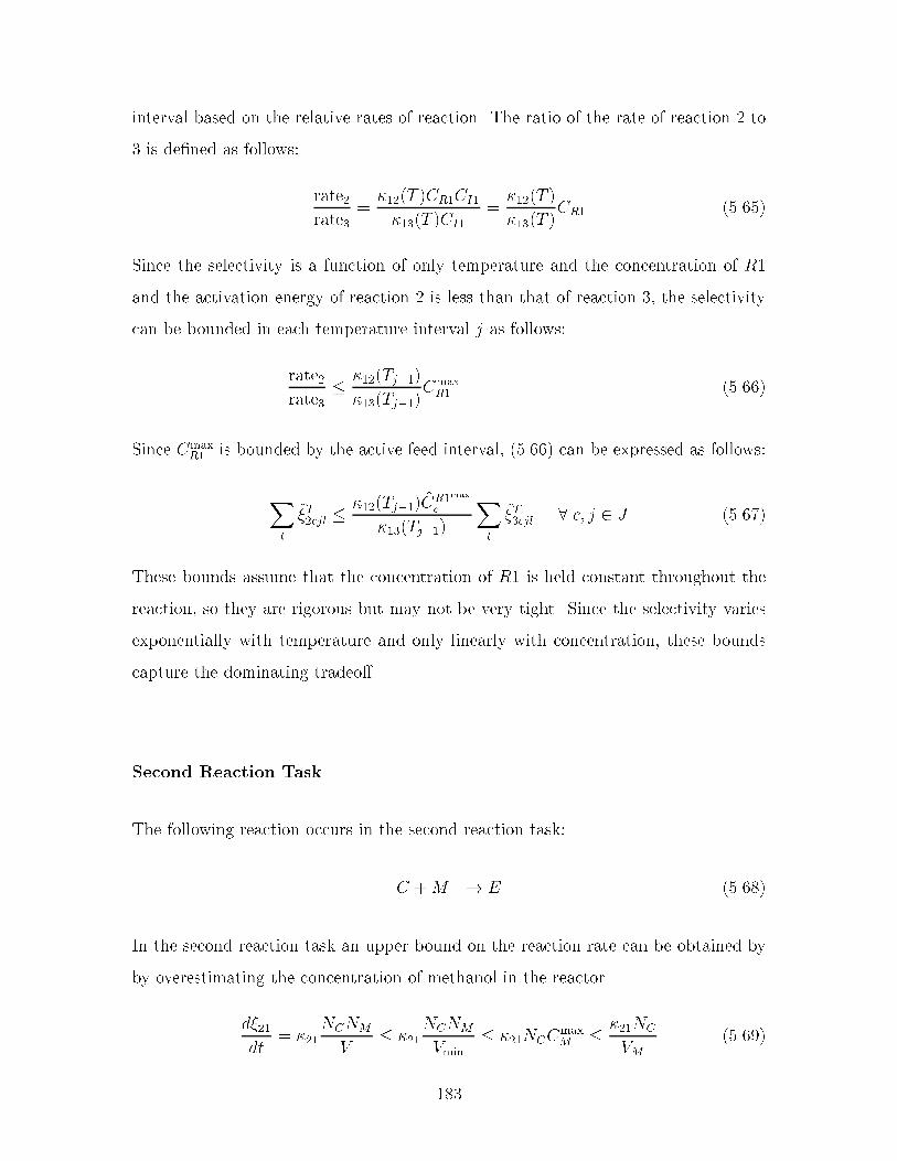
interval based on the relative rates of reaction The ratio of the rate of reaction � to
� is de�ned as follows�
rate�rate�
� ���T �CR�CI�
���T �CI�
� ���T �
���T �CR� �����
Since the selectivity is a function of only temperature and the concentration of R�
and the activation energy of reaction � is less than that of reaction �� the selectivity
can be bounded in each temperature interval j as follows�
rate�rate�
� ���Tj��� ���Tj���
CmaxR� �����
Since CmaxR� is bounded by the active feed interval� ����� can be expressed as follows�
Xl
(�T�cjl � ���Tj��� %CR�max
c
���Tj���
Xl
(�T�cjl � c� j � J �����
These bounds assume that the concentration of R� is held constant throughout the
reaction� so they are rigorous but may not be very tight Since the selectivity varies
exponentially with temperature and only linearly with concentration� these bounds
capture the dominating tradeo�
Second Reaction Task
The following reaction occurs in the second reaction task�
C "M � E �����
In the second reaction task an upper bound on the reaction rate can be obtained by
by overestimating the concentration of methanol in the reactor
d���dt
� ��NCNM
V� ��
NCNM
Vmin� ��NCC
maxM � ��NC
VM�����
���

We have employed the fact that the concentration of methanol cannot be greater
than the concentration of pure methanol� de�ned by the molar volume of the species
While this is a crude approximation� it is not too far �within �� #� from the initial
methanol concentration if there are no other solvents in the reactor� and it provides
a rigorous bound Therefore�
��� � fRin�C
��� e
����vM
tR�
�����
Since the second reaction task did not typically limit the cycle time� this bound was
deemed su�cient
For this reaction task� linear bounds are enforced by providing a piecewise constant
overestimation of the feasible region Since high conversion is required in this reactor�
the conversion is divided into intervals� and an SOS� set �ie�P
c yConvC
c � �� of binary
variables yConvC
c is employed to indicate in what range the conversion achieved lies
Denoting the upper and lower bounds on the conversion in each interval by %xCUP
c and
%xCLO
C respectively� the active region can be identi�ed as follows�
Xc
yConvC
c %xCLO
c fRin�C � ��� �Xc
yConvC
c %xCUP
c fRin�C �����
The bilinear terms are replaced by introducing a new variable NCc � fRin�C yConv
C
c
de�ned using an exact linearization A lower bound on the time required to achieve
��� is given as follows�
tR� �Xc
yConvC
c
ln��� %xC
LO
c
� ��VM �����
Third Reaction Task
The third reaction task converts intermediate E into product D The reaction is
carried out in a large excess of water �at least �� times E� This reaction is restricted
to temperatures below �� C� so an upper bound on the rates that can be achieved is
imposed by this temperature Since the reaction is second order in E� the rates will
���

be maximized if the same material is contained in a smaller volume This implies
that the rate can be overestimated by assuming no dilution by inert materials� by
underestimating the volume during the entire reaction� and by assuming that all
the reactants are available initially The volume increase upon reaction is ignored
to overestimate the rate of reaction If the reaction is carried out isothermally� the
reaction time can be related to the conversion of E as follows�
� ��tR� �
�
CE� �
CEo
�Vf
��� xE�NEo
� VoNEo
� VoNEo
��
�� xE� �
������
An underestimate of the time required to achieve a given conversion occurs can be
derived from ����� by assuming the reactor is operated at the maximum temperature
for the duration of the reaction and by underestimating the VoNEo term by assuming
the concentration of E is not diluted by excess water or other components
tR� ��
�
�� xE� �
��VE " ��VW
� max��
������
In ����� max�� denotes the value of the rate constant at �� C
Equation ����� can be used to derive a simple lower bound on the reaction time in
the same fashion used to derive a lower bound for the processing time of the second
reaction The conversion that is achieved in the reactor is restricted to lie in one
of several intervals that cover the range of feasible conversions for this reaction� a
SOS� set of binary variables yConvE
c �ie�P
c yConvE
c � �� is employed to indicate in
what range the conversion achieved lies Denoting the upper and lower bounds on
the conversion in each interval by %xEUP
c and %xELO
c respectively New variables NEc �
fRin�E yConvC
c are de�ned using an exact linearization in order to relate the conversion
to the extent of the reaction
Xc
NEc %xE
LO
c � ���� �Xc
NEc %xE
UP
c �����
A lower bound on the time required to achieve ��� is given by replacing the xE in
���

����� with the lower bound of the active conversion interval�
tR� ��VE " ��VW
� max�
�Xc
yConvE
c
��
�� %xELO
c
� �
������
���� Solutions to Case Study II
The screening model was employed to determine the minimum cost design for the pro
duction of siloxane monomer In determining the minimum cost design the screening
model determines whether the downstream processing to convert C into D is cost
e�cient Two superstructures were considered in this case study The �rst includes
only the �rst reaction task� and the second requires all three The screening model
will select between these two options if it is allowed to decide whether the reaction
tasks should be performed or not� but solving the problem using two di�erent su
perstructures allows us to compare the optimal screening solution derived from each
superstructure� rather than simply �nding out which structure leads to the best so
lution In addition� it reduces the combinatorial complexity of the model
Lower bounds on the manufacturing cost for ������� kg of product are determined
for each superstructure Raw material� waste disposal� utility� and equipment rental
costs were considered for a manufacturing campaign employing no intermediate stor
age� end e�ects were ignored The product was required at a purity of ��# de�ned
on a mass basis Two percent of all recycled material was purged Material transfers
are assumed to take � hours� and � hours are required to bring the columns to total
re ux before drawing product The solutions obtained for each of the superstructures
are described in the next two sections
Eight temperature intervals de�ned by ����� ���� ���� ���� ���� ���� ���� ����
��� K� were employed when deriving the targets for the �rst reaction task Five feed
intervals were employed The upper bound on the �rst four feed intervals represent
increases of � # over the minimum amount of R� required to achieve the required
production The ratio of R� to R� was partitioned into �ve intervals� with the upper
bounds on the �rst four intervals de�ned by ��� ��� ��� and ��
���

Case II A� One Reaction Task Allowed
A lower bound on the manufacturing cost of �����kg was obtained using only one
reaction and one distillation task A schematic of the solution is provided in �gure ��
The streams are labeled with the material ows for the entire campaign for each of the
�xed points contained in the stream Since �� batches are employed in this campaign�
the amounts charged during each batch can be determined from the �gure ��
The solution of the screening model for the three reaction process� chooses not to
perform any of the second and third reactions even though we imposed constraints
that required equipment to be assigned to the third reaction and distillation tasks
Hence� it cost more that the solution above
*333
5,
5*
6
-./+*
*343+,
,.+2
�7,+/
*333
�-.,+/
56
6
-+2
*.+2
#�����7+2
�
5*
6
�
*+4
*22+,
23*+*
-.,+/
56
6
,2.+4
142+3
Figure ��� Process schematic of the solution derived from the superstructure containing only one reaction task Streams labels denote the ow of each �xed point inkmols for the campaign
The reaction task employs the ���� gallon reactor and converts all of the R�
charged into A and C� with no I� left unreacted The reactor operates for a total
���
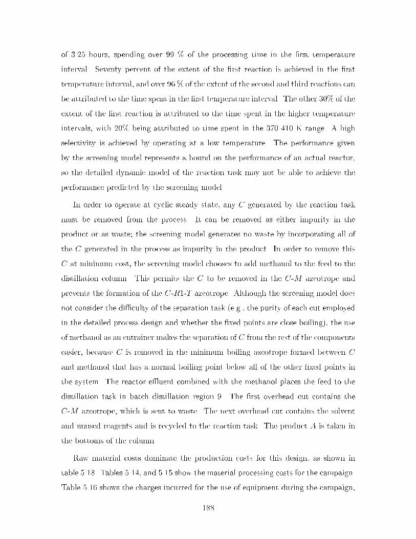
of ��� hours� spending over �� # of the processing time in the �rst temperature
interval Seventy percent of the extent of the �rst reaction is achieved in the �rst
temperature interval� and over �� # of the extent of the second and third reactions can
be attributed to the time spent in the �rst temperature interval The other ��# of the
extent of the �rst reaction is attributed to the time spent in the higher temperature
intervals� with ��# being attributed to time spent in the ������ K range A high
selectivity is achieved by operating at a low temperature The performance given
by the screening model represents a bound on the performance of an actual reactor�
so the detailed dynamic model of the reaction task may not be able to achieve the
performance predicted by the screening model
In order to operate at cyclic steady state� any C generated by the reaction task
must be removed from the process It can be removed as either impurity in the
product or as waste� the screening model generates no waste by incorporating all of
the C generated in the process as impurity in the product In order to remove this
C at minimum cost� the screening model chooses to add methanol to the feed to the
distillation column This permits the C to be removed in the CM azeotrope and
prevents the formation of the CR�T azeotrope Although the screening model does
not consider the di�culty of the separation task �eg� the purity of each cut employed
in the detailed process design and whether the �xed points are close boiling�� the use
of methanol as an entrainer makes the separation of C from the rest of the components
easier� because C is removed in the minimum boiling azeotrope formed between C
and methanol that has a normal boiling point below all of the other �xed points in
the system The reactor e)uent combined with the methanol places the feed to the
distillation task in batch distillation region � The �rst overhead cut contains the
CM azeotrope� which is sent to waste The next overhead cut contains the solvent
and unused reagents and is recycled to the reaction task The product A is taken in
the bottoms of the column
Raw material costs dominate the production costs for this design� as shown in
table ��� Tables ���� and ��� show the material processing costs for the campaign
Table ��� shows the charges incurred for the use of equipment during the campaign�
���

and table ��� shows the utilization of the equipment The batch size and cycle time
are the same for both tasks
Raw Material CostsRaw Material Cost &� � kg' Feed &kg' Total Cost &�' � � kg product
M ��� ���� ���� ���R� ��� ������� �������� ���R� ��� ������� �������� ���T ��� ������ ������ ���
Total �������� �������� ���
Table ���� Raw material costs for the entire campaign for the process containingonly one reaction task
Utility CostsCut Material Amount & kg ' Reboiler Cost &�' � � kg product
Distillation �CM ����� ��� ���RT ������� ��� ���T ������� ��� ���
Total ������� ��� ���
Table ���� Utility costs for the distillations for the entire campaign for the processcontaining only one reaction task
Case II B� All Reaction Tasks Required
A lower bound on the manufacturing cost of �����kg is obtained when all we require
that all three reaction tasks are performed In order to ensure that all the reactions
are performed� we require that at least ��# of the C generated in the �rst reaction
is converted to E in the in the second reaction� and we require that at least ��# of
the E is converted into D A schematic of the solution is provided in �gure �� The
streams are labeled with the material ows for the entire campaign for each of the
�xed points contained in the stream Since �� batches are employed in this campaign�
the amounts charged during each batch can be determined from the �gure ��
���

*3334-3 4-3
������
5,
5*
6
-.,+4
*314+1
*1+3
-33 4-3
56
6
-+2
*/+3
�7,+/
-33
)�,+*
�-.*+*
�
7
5*
6
�
*+4
+2
*24+4
400+*
-.*+*
�+2
7
)
+*
-0+-
7
)
�
�
/+0
13+1
+,
+2
)-2+1
)�
+3/
7+*
7+2
7/+*
56
6
,2.+3
12/+*
Figure ��� Process schematic of the solution derived from the superstructure requiring all three reaction tasks Streams labels denote the ow of each �xed point inkmols for the campaign
���

Reactor Rental CostsVolume Assigned Rental Rate Total Cost � per&gal' Units & � � hr' & � ' kg product���� � �� ������� ���
Distillation Column Rental CostsVolume Vapor Rate Assigned Rental Rate Total Cost � per&gal' & kmol�hr ' Units & � � hr' &�' kg product���� �� � ��� ������� ���
Total for reactors and columns ������� ���
Table ���� Equipment costs for the entire campaign for the process containing onlyone reaction task
Utilization Processing TaskMeasure Reaction � Distillation �
Cycle Time ��� ���Volume Required ����� �����Volume Assigned ������ ������
Table ���� Equipment utilization for the design obtained from the process containingone reaction task
Cost ContributionsComponent Percent Total Cost &�' � � kg productRaw Material ���� �������� ���Waste Disposal ��� ��� ���Utility ��� ��� ���Equipment ��� ������� ���Total �������� ���
Table ���� Comparison of raw material� waste disposal� utility� and equipment costsfor the process containing only one reaction task
���

The �rst reaction task employs the ��� and ��� gallon reactors and converts all of
the R� charged into A and C� with no I� left unreacted The reactor operates for a
total of ��� hours� spending over �� # of the processing time in the �rst temperature
interval Roughly seventy percent of the extent of the �rst reaction is achieved in
the �rst temperature interval� and over �� # of the extent of the second and third
reactions can be attributed to the time spent in the �rst temperature interval The
other ��# of the extent of the �rst reaction is attributed to the time spent in the
higher temperature intervals A high selectivity is achieved by operating at a low
temperature The operation of the �rst reactor given by the solution is very similar
to the reactor operation for Case IIA However� in this case� we require that the C
generated in the �rst reactor is processed to product D
The e)uent from the �rst reactor is separated using both ��� gallon distillation
columns The columns operate in batch distillation region �� note that the methanol
recycled from the third distillation to the �rst reactor acts as an entrainer A is taken
in the bottoms of the column� the CM azeotrope is passed on to the second reaction�
and the unused reagent and solvent are recycled
The second and third reaction tasks are merged into a single equipment stage
that employs a ��� gallon reactor The e)uent from these reaction tasks is separated
in the ���� gallon distillation column Since very little C is generated in the �rst
reaction and the manufacturing facility does not contain any reactors and columns
an order of magnitude smaller� these equipment items are underutilized as shown in
table ���
As with study case IIA� raw material costs dominate the production costs for this
design� as shown in table ��� Tables ��� and ��� show the material processing costs
for the campaign Table ��� shows the charges incurred for the use of equipment
during the campaign The batch size and cycle time are limited by the �rst reaction
task
���

Raw Material CostsRaw Material Cost &� � kg' Feed &kg' Total Cost &�' � � kg product
M ��� ��� ��� ���R� ��� ������� �������� ���R� ��� ������� �������� ���W ��� ������ ���� ���T ��� ������ ������ ���
Total �������� �������� ���
Table ���� Raw material costs for the entire campaign for the process requiring threereaction tasks
Utility CostsCut Material Amount & kg ' Reboiler Cost &�' � � kg product
Distillation �CM ����� ��� ���RT ������� ��� ���T ������� ��� ���
Distillation �M ����� ��� ���WE ���� ��� ���W ������ ��� ���
Total ������� ��� ���
Table ���� Utility costs for the distillations for the entire campaign for the processrequiring three reaction tasks
Comparison of the two superstructures
The design that requires that all three reaction tasks are performed results in higher
manufacturing costs than the design with only one reaction task Although the three
reaction process has slightly lower raw material costs� this savings is outweighed by
the additional equipment cost incurred by dedicating a reactor and column to the
downstream processing for the duration of the campaign Thus� the one reaction
task design is more desirable if this high selectivity can be achieved through dynamic
optimization of the operating policy of the �rst reaction
The screening model superstructure used in this example did not consider employ
���

Reactor Rental CostsVolume Assigned Rental Rate Total Cost � per&gal' Units & � � hr' & � ' kg product��� � �� ������� ������ � �� ������� ���
Distillation Column Rental CostsVolume Vapor Rate Assigned Rental Rate Total Cost � per&gal' & kmol�hr ' Units & � � hr' &�' kg product��� �� � �� ������� ������� �� � ��� ������� ���
Total for reactors and columns ������� ���
Table ���� Equipment costs for the entire campaign for the process requiring threereaction tasks
Utilization Processing TaskMeasure Rxn � Dist � Rxn � Rxn � Dist �
Cycle Time ��� ��� ��� ��� ���Volume Required ������ ������ ��� ���� ����Volume Assigned ������ ������ ����� ����� ������
Table ���� Equipment utilization for the design obtained from the process requiringthree reaction tasks
Cost ContributionsComponent Percent Total Cost &�' � � kg productRaw Material ���� �������� ���Waste Disposal ��� ��� ���Utility ��� ��� ���Equipment ��� ������� ���Total �������� ���
Table ���� Comparison of raw material� waste disposal� utility� and equipment costsfor the process containing only one reaction task
ing intermediate storage or the possibility of changing the operation of the process at
some point during the campaign �ie� using an item of equipment for di�erent tasks
at di�erent times�� so the downstream items of equipment are underutilized The
���

use of intermediate storage alone will not improve the equipment utilization much
since the same task already limits both the batch size and cycle time� but if we relax
the restriction that equipment items are dedicated to a particular task for the entire
campaign� a process employing three reaction tasks may become more attractive For
example� if su�cient intermediate storage is available� we might consider operating
the �rst reaction and distillation tasks as suggested by the solution of the screening
model and storing the C �M azeotrope until all the batches of the �rst two tasks
are completed At this point� the same equipment could be employed for the second
and third reactions and �nal distillation Although the use of intermediate storage is
considered by the screening models formulated in chapter �� extensions to the screen
ing model are required to consider process that do not operate in campaign mode
�ie� those in which equipment items are not dedicated to a particular task for the
duration of the campaign�
���� Case III� Disposing of Recycle Streams
This example considers the cost of disposing of recycled material at the completion
of the campaign We employ the reaction targets described above and consider the
process containing only one reaction task The trade o� between the size of the
batches and the campaign length is considered
We assume that the amount of material recycled per batch must be disposed of
at the conclusion of the campaign� unless this material is one of the raw materials
used by the process The cost of disposing of this material is added to the objective
function� and the cost to manufacture ������� pounds of monomer is minimized
The solution of the screening model results in a process that di�ers from the
one obtained when the disposal of the recycle streams was not considered This
design employs �� batches� instead of ��� to manufacture the product at a cost of
�����kg A smaller reactor is employed and the cycle time of the process is reduced�
but the campaign length is increased from ��� to ��� hours Raw material costs are
identical between this design� shown in �gure ��� and the design shown in �gure ��
Tables ������� show the raw material� waste disposal� utility� and equipment rental
���
costs All of the waste generated results from the disposal of the recycle streams We
assume that the recycled toluene� one of the raw materials� can be reused in another
process� so no cost is assessed for this recycle Although the distillation column is
larger than necessary as shown in table ���� using the ���� gallon column reduces the
cycle time because it has the largest vapor rate of the available columns Table ���
shows breakdown of the processing costs� demonstrating that the raw material costs
still dominate
4-3
5,
5*
6
-./+*
*343+,
,.+2
�7,+/
*333
�-.,+/
56
6
-+2
*.+2
#�����7+2
�
5*
6
�
*+4
*22+,
23*+*
-.,+/
56
6
,2.+4
142+3
Figure ��� Process schematic of the solution derived from the superstructure containing only one reaction task in which the disposal of recycle streams at the endof the campaign is considered Stream labels indicate the �xed point ows for thecampaign given in kmols
�� Conclusions
Computationally tractable models can be derived that provide bounds on the cost of
manufacture for processes commonly encountered by synthetic pharmaceutical and
���

Raw Material CostsRaw Material Cost &� � kg' Feed &kg' Total Cost &�' � � kg product
M ��� ���� ���� ���R� ��� ������� �������� ���R� ��� ������� �������� ���W ��� ��� ��� ���T ��� ������ ������ ���
Total �������� �������� ���
Table ���� Raw material costs for the process considering the disposal of recycledmaterial at the completion of the campaign
Waste Disposal CostsWaste Material Cost &� � kg' Amount &kg' Total Cost &�' � � kg product
RT ���� ����� ������ ���Total ����� ������ ���
Table ���� Waste disposal costs for the process considering the disposal of recycledmaterial at the completion of the campaign
Utility CostsCut Material Amount & kg ' Reboiler Cost &�' � � kg product
Distillation �CM ����� ��� ���RT ������� ��� ���T ������� ��� ���
Total ������� ��� ���
Table ���� Utility costs for the distillation task in the process considering the disposalof recycled material at the completion of the campaign
specialty chemical manufacturers These models embody many of the processing
limitations governing the process design� yet they are able to consider continuous and
discrete aspects of the design simultaneously They also enable some of the process
synthesis decisions to be systematically considered during the design procedure The
screening models do not consider the process dynamics� so these models must be used
���

Reactor Rental CostsVolume Assigned Rental Rate Total Cost � per&gal' Units & � � hr' & � ' kg product��� � �� ������� ���
Distillation Column Rental CostsVolume Vapor Rate Assigned Rental Rate Total Cost � per&gal' & kmol�hr ' Units & � � hr' &�' kg product���� �� � ��� ������� ���
Total for reactors and columns ������� ���
Table ���� Equipment costs for the process considering the disposal of recycledmaterial at the completion of the campaign
Utilization Processing TaskMeasure Reaction � Distillation �
Cycle Time ��� ���Volume Required ����� �����Volume Assigned ����� ������
Table ���� Equipment utilization for the process considering the disposal of recycledmaterial at the completion of the campaign
Cost ContributionsComponent Percent Total Cost &�' � � kg productRaw Material ���� �������� ���Waste Disposal ��� ������ ���Utility ��� ��� ���Equipment ��� ������� ���Total �������� ���
Table ���� Comparison of raw material� waste disposal� utility� and equipment costsfor the process considering the disposal of recycled material at the completion of thecampaign
in conjunction with detailed dynamic simulation or pilot plant experiments However�
the solution of the screening models facilitates the cyclic steady state simulation of
a dynamic process containing recycles and the formulation of a multistage dynamic
���

optimization of the process by providing both initial estimates of the owrates in the
process and alternative process structures
The solution of the process development example demonstrates that integrated
processes employing recycles can signi�cantly reduce the waste generated during the
manufacture of these products The process operates at cyclic steady state� so the
recycled material does not accumulate However� at the conclusion of the campaign�
this material must either be stored inde�nitely� or sent to a recovery facility As
demonstrated by the process development example the amounts that are recycled
can be on the same order as the total waste generated during the campaign The end
e�ects of the campaign are important from the standpoint of pollution prevention
and may possibly impact the design from a cost standpoint as well Section ���
shows that if the number of batches is not very large� the cost of waste disposal at
the conclusion of the campaign can a�ect the way in which the process is operated�
trading o� operating and waste costs
As in chapter �� the screening models demonstrate the ability to perform some
aspects of the process synthesis In fact� the results of the case study II demonstrate
that the process employing only one reaction task is potentially more e�cient than
one that contains the downstream processing to convert C to D� However� detailed
dynamic models are required to perform an accurate comparison of the costs� but the
solutions of the screening model provides good initial guesses for a material states
involved in the dynamic optimization of the process performance
This chapter also highlights the need to extend the screening formulations to han
dle both reactive distillation processes and heterogeneous mixtures These examples
assume that reaction does not occur in the distillation columns� although some reac
tion must occur This was not a limitation in chapter � since the reactions employed
a heterogeneous catalyst which was �ltered before entering the distillation columns
�A complete comparison requires the detailed design� but the one reaction process will be moree�cient provided that a su�ciently high conversion of A versus C can be achieved using detaileddynamic optimization of the reaction I operating policy�
���

���

Chapter �
Numerical Issues in the Simulation
and Optimization of Hybrid
Dynamic Systems
Section �� described the need to employ hybrid discrete�continuous modeling envi
ronments for the detailed simulation and optimization of batch processes A key to
the application of modeling technology to the design of batch processes has been the
evolution of equationbased simulation tools� such as SpeedUp �AspenTech� ������
ASCEND �Westerberg et al�� ������ POLYRED �Ray� ������ or ABACUSS �Barton�
������ into process modeling environments in which a common reusable process model
may be used reliably for a variety of di�erent computational tasks �Pantelides and
Barton� ������ such as both steadystate and dynamic simulation� optimization� sensi
tivity analysis� uncertainty analysis� etc Such environments decouple the description
of the process model from the solution procedure� yielding major advantages for the
user of the system The user is free to concentrate on the correct formulation of the
model and simulation experiment rather than the details of the numerical solution
procedures� thus� the user need not be an expert in numerical analysis While this is
a desirable goal� it places stringent demands and high expectations on the robustness�
accuracy� and generality of the solution procedures For example� our experience with
the application of the stateoftheart numerical algorithms employed within ABA
���

CUSS to the batch distillation of wideboiling azeotropic mixtures has demonstrated
that the numerical technologies have not yet attained the level of robustness required
for the routine simulation and optimization of batch processes
The following chapters focus on improvements to the robustness and e�ciency of
the numerical algorithms employed within the ABACUSS process simulator Two
main areas have been investigated� �� improving the accuracy and robustness of
the integration procedure for models that become locally illconditioned during the
course of the transient� and �� improving the e�ciency of the integration algorithm
during the initial phase of the integration procedure These improvements have been
incorporated within an integration code designed for the integration of large sparse
unstructured systems of di�erentialalgebraic equations called DSL��S �Feehery et al��
����� Therefore� although the development of these techniques has been motivated
by the needs of hybrid discrete�continuous simulation environments� the techniques
apply to general sparse unstructured systems of DAEs
�� Accuracy of Solution Procedures
Mathematical models provide a formalism with which to encapsulate our understand
ing of the physical world and apply this knowledge to calculations of engineering
interest The derivation of useful models comprises two tasks� a� identifying the
physical phenomena relevant to the current engineering activity� and b� accurately
representing this phenomena within the mathematical formalism Identifying the rel
evant phenomena permits the model to capture important behavior in the physical
process without obscuring the results in a sea of detail and without burdening the
computation with unnecessary calculations Accurately capturing the relevant phe
nomena within the mathematical model is critical to the utility of the simulation
results The derivation of good models remains a di�cult task� but process model
ing environments provide a framework in which to apply these models to a variety
of engineering calculations In fact� a single reusable mathematical model can be
employed for engineering calculations performed over the lifetime of a process �Bar
���

ton� ����� However� the user of such an environment expects the results provided
from all simulations to meet certain minimal accuracy requirements While any user
recognizes that the numerical solution is an approximation of the exact solution of
the mathematical model� the solution should be a good approximation to the exact
solution
The �rst question to ask is how should the quality of the numerical solution
be measured In most cases� a numerical approximation that is close to the exact
solution is desired� letting x� de�ne the exact solution and x de�ne its numerical
approximation� a close solution is one that satis�es kx� � xk� � � where � is the
tolerance This de�nition also requires speci�cation of the norm� which could be the
maximum norm� the two norm� or any other norm that is desired The norm re ects
both the knowledge about the expected solution �eg� are all the variables on the
same scale � and any requirements that the solution should satisfy �eg� should some
average property be enforced� or does every component of the solution need to satisfy
a requirement in order to employ the solution for engineering purposes� The norm
should also indicate whether we require relative accuracy in the solution or whether
we require that some absolute tolerances are achieved The di�erence between the
exact and the calculated solution is referred to as the forward error of the solution
Usually� a small forward error would satisfy our expectations However� in other
cases we may require that we have found a solution that achieves small residuals For
instance in an interpolation problem we are likely to be more interested in whether the
solution provides a good approximation of the data �either in an absolute or relative
sense� rather than how well it approximates the exact solution of the problem In
many cases� bounds relating these quantities are easily derived �Higham� �����
Di�erences between the numerical solution of our mathematical model and the
performance of the process being modeled come from several sources�
� Approximations made during the abstraction of the physical process into a
mathematical model
� Errors in the problem data These errors may be attributed to imprecise mea
���

surements of physical quantities �eg� VLE or property measurements�� the
error in a previous calculation �eg� parameter estimation�� or they may simply
be the result of representing an exact quantity in �nite precision
� Truncation error arising from terminating an exact approximation �such as a
Taylor series� after a �nite number of terms In many cases� the truncation error
is a function of the discretization �ie� the step size and order of a numerical
integration�
� Rounding errors arising from the fact that the computations are carried out on
machines of �nite precision
The users of process modeling environments typically expect that the applicability
of their simulation results depends on the errors attributed to the abstraction of the
physical process� and the errors in the measured data incorporated in the model such
as the parameters employed to predict physical properties It is the user�s duty to
make certain that these approximations are valid and apply the results with an under
standing of the potential inaccuracies Some process modeling environments ease the
interpretation of uncertainty in the problem data by calculating the sensitivity of the
results to perturbations in the problem data �Barton and Gal*an� ����� Tatang� �����
The user expects the contributions of the other error components to be controlled by
the numerical solution procedure to achieve the requested accuracy The user indi
cates the desired solution accuracy by specifying the tolerance for the computations
This tolerance is then typically used to control the truncation error� balancing the
speed of computation with the need for accuracy
While simulating the batch distillation of wideboiling azeotropic mixtures� we
have uncovered situations where the implicit assumption that the e�ect of rounding
errors is negligible certainly breaks down� �gure �� provides a dramatic illustration
of this phenomenon While the simulation results appear to predict the dominant
processing characteristics correctly �ignoring the spikes�� large contributions of the
rounding errors were witnessed as spikes in the values of certain variables� without any
accompanying warnings being issued by the numerical routines �except in cases where
���

the algorithms simply failed� This highlights a major problem for the application
of the results The results clearly do not meet the desired accuracy requirements�
but the numerical procedures do not provide any indication that this has occurred
The uninformed user may then go on to employ these results as if they were correct
Since detailed dynamic models of chemical processes are employed for the design of
operating policies �Ochs et al�� ������ control strategies �Zitney et al�� ������ and the
speci�cation of equipment �Naess et al�� ������ the application of incorrect results
can waste money Even worse� these results may be used to verify the safety of
proposed operating procedures� or the safety of the process under abnormal operating
conditions �Sedes� ����� Although we have not encountered situations where these
errors have changed the qualitative behavior of the simulation� it is not hard to
imagine that the perturbations of the variables that have been witnessed could cause
the improper identi�cation of state events� changing the functional form of the model
and leading to very di�erent qualitative behavior �Park and Barton� ����� In other
cases� the breakdown in the control of the accuracy is not signaled by a large deviation
in a variable value� but rather a failed simulation While this result is also not
desirable� at least the results are not likely to be interpreted as if they are correct
Condenser Duty versus Time
Q [J/S]
Duty [Joules/sec] x 103
3Time x 10
-120.00
-100.00
-80.00
-60.00
-40.00
60.00 80.00 100.00 120.00 140.00
Condenser Duty versus Time
Q [J/S]
Duty [Joules/sec] x 103
3Time x 10
-113.50
-113.40
-113.30
-113.20
-113.10
-113.00
-112.90
-112.80
-112.70
-112.60
-112.50
-112.40
-112.30
-112.20
-112.10
-112.00
-111.90
-111.80
94.66 94.66 94.66 94.66 94.66 94.66 94.66 94.66
Figure ��� Plot of condenser duty resulting from ABACUSS simulation showing one�spike� in detail
It is unreasonable to expect that any level of accuracy can be achieved using
���

�nite precision computations� However� numerical algorithms should make attempts
to mitigate the e�ects of rounding errors �many e�ective algorithms are backward
stable� guaranteeing a solution with small backward error�� and warn users when
the desired accuracy has not been maintained due to the e�ects of rounding error
and the conditioning of the problem As we shall prove in chapter �� the problems
we have observed are the result of illconditioning We have found that automatic
scaling of the equations and variables during the integration procedure improves the
performance of the numerical algorithms and permits evaluation of the accuracy of the
solution Not only does this allow the computation to maintain the desired accuracy�
but also improves the robustness and e�ciency of the method Before addressing
the results contained in chapter �� some background on conditioning and linear error
analysis may prove useful
����� Backward Error and Conditioning
Finite precision arithmetic imposes barriers on the accuracy that can be achieved due
to the e�ects of the rounding errors Even if the computations could be carried out
exactly� rounding errors are encountered merely by representing the problem data in
�nite precision Wilkinson ������ recognized that the solution obtained by a numer
ical calculation in �nite precision arithmetic is equivalent to the exact solution of a
similar problem with perturbed data� the size of these perturbations is termed the
backward error The backward error interprets the errors committed during the cal
culation as perturbations of the problem data Since errors in the problem data are
encountered just from storing the problem� if the backward error is of that order we
can hope to do no better during the calculation The second motivation for bounding
the backward error is that the relationship between the backward and forward errors
of the problem can be determined from perturbation theory Perturbation theory
is understood for many problems �Stewart and Sun� ������ an advantage of pertur
bation analysis is that it is a characteristic of the problem and not the algorithm
�It is assumed that the computations are employing the machine�s standard arithmetic operationsand are not simulating arithmetic of arbitrarily high precision Higham� � ���
���

Backward error analysis possesses advantages over direct roundo� analysis� where
each algebraic computation is regarded as an operation which approximates the true
algebraic process By using the backward or inverse roundo� analysis� the analysis
of the solution procedure can be undertaken assuming the standard algebraic axioms
In contrast� in direct roundo� analysis the multiplication and addition operations
do not follow either the associative or distributive laws Thus� an entirely di�erent
system of analysis must be devised
The relationship between the forward and backward errors is given by the condi
tioning of the problem The conditioning of a problem measures the sensitivity of the
solution of the problem to perturbations in the problem data� so it is a function of the
problem and not the solution algorithm For scalar functions� the relative condition
number measures the relative change in the output caused by a relative change in
the input For vector functions the changes are measured using a suitable norm� and
the condition number measures the maximum relative change in the output caused
by a relative change in the input The maximum change in the output is achieved
by some� but not all� input perturbations When the forward error� backward error�
and the condition number are de�ned in a consistent fashion� the following rule of
thumb �Higham� ����� demonstrates that an illconditioned problem can lead to a
large forward error even if small backward is achieved�
forward error � condition number � backward error ����
The conditioning of the linear systems solved during the corrector iteration of the
BDF code indicate that large error in the values of some of the variables can be ob
tained even when the residuals are evaluated accurately� and the Gaussian elimination
produces small backward error Rounding error analysis and conditioning of linear
systems is reviewed in section ���
���

�� E�ciency of Integration Codes
The routine simulation and optimization of large DAE models containing discon
tinuities will only be realized once the solution algorithms and computer hardware
enable these calculations to be performed in reasonable time on desktop workstations
When using BDF integration codes �see section ����� the computation time of the
solution algorithm is dominated by the time spent factoring the corrector iteration
matrix Thus� the number of times the matrix is factored and the e�ciency of the
linear algebra used to factor the matrix dictate the e�ciency of the BDF code Nu
merical analysts have devoted years of e�ort developing e�cient codes to factor the
large sparse unstructured matrices that are obtained during the dynamic simulation
of chemical processes �Du� and Reid� ����� Zitney� ����� Zitney and Stadtherr� �����
Zitney et al�� ������ so these algorithms will not be examined here The heuristics
employed within the implementation of the BDF method contained in a particular
code typically seek to minimize the number of times the corrector iteration matrix is
factored Since the need to factor the matrix depends on the changes in the variable
values and the change in the step size� it is important that the step size is on scale
for the problem
This thesis proposes two techniques to keep the step size on scale for the problem
First� the automatic scaling technique described in chapter � mitigates the e�ects of
illconditioned models in order to avoid situations in which the step size is cut unnec
essarily due to inaccurate solutions of the corrector In addition� chapter � develops
a method to determine an initial step size that is on scale for the problem which is
required at the start of the simulation or following any discontinuity Although both
techniques bene�t all dynamic models� the second technique is most applicable to
simulation and optimization of hybrid dynamic systems because these calculations
require the integration code to be started many times during a single simulation or
optimization experiment
���

�� Mathematical Background
Since the focus of this thesis is the application of mathematical modeling technology
to the design of batch processes� the reader is likely to be more interested in the
bene�ts provided by improvements to the numerical algorithms than the details of
the numerical analysis required to develop the new solution procedures However�
some details of the numerical analysis are required to understand both the motiva
tion and the application of the techniques developed in the following chapters This
section describes the components of the integration algorithm on which our numerical
advances have focused� and provides background that is required to understand the
following chapters for the reader who has not devoted a career to numerical analysis
����� BDF Integration Codes
Backward di�erentiation formula �BDF� methods are a class of linear multistep meth
ods suitable for the solution of sti� ODE systems and index� DAEs �Gear� �����
In particular� BDF methods can solve DAEs expressed in fully implicit form ����
directly
f� $z� z� t� � � ����
The kth order BDF method approximates the time derivative of the solution $z�t�
using the derivative of a kth order polynomial that approximates the solution z�t�
over the last k " � points �including the current point� The simplest BDF method
is equivalent to the implicit Euler method in which $z is replaced by the �rst order
backward di�erence approximation This reduces the system of equations that must
be satis�ed at every time step to the following�
f�zn � zn��hn��
� zn� tn� � � ����
where hn�� � tn � tn�� denotes the length of the integration step and zn denotes the
numerical approximation to the solution at tn For higher order BDF methods� the
���
equations solved at each time step can be written as follows �Brenan et al�� ������
f��zn " �� zn� tn� � � ����
where � is a constant that depends on the order of the approximation and the step size�
and � is a constant that contains the contributions of the solution from previous steps
to the BDF approximation of $z�tn� Although many other methods have been applied
to the solution of index� DAEs� the greatest success has been achieved from codes
based on BDF methods� probably due to their large regions of absolute stability and
high accuracy �Brenan et al�� ����� Several texts describe the theoretical properties
of these methods in detail �Lambert� ����� Hairer and Wanner� ����� Brenan et al��
�����
The BDF codes examined within this thesis are implemented using a predictor
corrector scheme that automatically adjusts both the step size and the order of the
approximation The BDF method requires the solution of the system of nonlinear
equations given by ���� at each time step� which is solved using a modi�ed version
of Newton�s method BDF predictorcorrector methods employ an explicit predictor
based on extrapolation of the BDF polynomial approximation of the solution to pro
vide an initial value for the iterative procedure used to determine the solution of the
nonlinear equations zn at tn The equations are converged in what is referred to as
the corrector iteration For convenience� we de�ne zPn and zCn as the predicted and
corrected solutions� note that zCn is the �nal Newton iterate� and not the exact solu
tion of the model equations at tn After zCn has been determined� the quality of the
approximation of the derivatives over the step is evaluated The step is accepted if
the approximation� measured an approximation of the local truncation error� is good
If the approximation is poor� then the step is rejected� and the integrator attempts
another step of smaller size� noting that the approximation should be exact as the
step size approaches zero
A owchart of the BDF integration algorithm is given in �gure �� We will ex
amine the calculations performed at each step in this algorithm in more detail below
���

�������������������� ����� �����������
����� ������ �� �
������������������
������������������� ����� � ��� ������ ��� �����
���� ��������� ��������� ���!������ ���!��
����� �����
� �� �� �� ���� ��"������� ��"����
����� #������� #��� �������� �������
$�����$���������������
��� ���� �������
��������������%��������%��������
%�
��
������������������� ����� � ��� ������ ��� �����
�������� ���� &�� �������� ���� &�� $ �� � ���� �� ����$ �� � ���� �� ����
�����������������������'�� ����'�� �
������
%�
%�
��
��
Figure ��� Flowchart for the predictor corrector implementation of the BDF method
Since factorization of the corrector iteration matrix is expensive� these algorithms em
ploy the factored matrix from a previous integration step until the convergence rate
of the corrector deteriorates or the step size changes substantially� either situation
indicates that the factored matrix is providing a poor approximation to the current
iteration matrix
Our analysis of the BDF method focuses on the solution of the nonlinear equations
performed by the corrector iteration We will also examine the truncation error
criteria to see how these criteria can be satis�ed when the corrector has been converged
numerically� yet zCn may still be far from the exact solution of the BDF equations at
tn However� we will not discuss the theory justifying the use of an approximation to
the local truncation error to control the error in the time evolution of the system� for
this� the reader is referred to other texts �Lambert� ����� Hairer and Wanner� �����
Brenan et al�� �����
Corrector Iteration
The corrector step in the BDF integration method solves the model equations for the
variable values� employing the BDF approximation to $z at the integration points At
time tn� the system of equations given by ���� is solved using a modi�ed version of
Newton�s method in which a deferred Jacobian is employed The corrector iteration
updates the value of zn at each step of the iteration �ie� zk��n � z
kn "�z
kn � using
���

the solution of the following linear system�
h�f�z
" �f� �z
� �z�z
i�zn �
h�f�z
" ��f� �z
i�zn � �f��zn " �� zn� tn� ����
The corrector iteration is continued until k�znkBDF � Tolerance This tolerance is
de�ned to be small enough so that the error incurred from terminating the Newton
iteration� will not be so large as to adversely a�ect the truncation error check For
example� the heuristics within DASSL require that the Newton iteration is converged
to within a tolerance that is one third the size of the permissible truncation error
�Brenan et al�� �����
Truncation Error Tolerance
The local truncation error is used to measure the accuracy of the backward di�erence
approximation to the derivatives DASSL also enforces a bound on the interpolation
error � the error in the solution interpolated between the integration points DASSL
estimates the truncation error using the principle term in the in�nite series expansion
of the local truncation error �Brenan et al�� ����� The interpolation error is estimated
in a similar fashion Both DASSL and DASOLV �Jarvis and Pantelides� ����� require
that the following condition is satis�ed before an integration step is accepted �Brenan
et al�� ������
error � M � ��zC � zP��BDF
� ��� ����
where zC is the corrected solution� zP is the predicted solution and M is a constant
that depends on the order of approximation and the current step size The user
requested integration tolerances are buried in the de�nition of the norm employed in
���� Let k�kBDF represent default norm used by the BDF integration routines to
measure the truncation error and size of the corrector updates It is de�ned in �����
�This error is also commonly referred to as truncation error� the error from truncating the in�niteseries of Newton iterates after a �nite number of iterations� but we will simply refer to it as thetermination error to avoid confusion with the local truncation error�
���
where zpi is the value of the variable zi from the previous integration step� �ri is the
relative error tolerance and �ai is the absolute error tolerance for variable i �Brenan
et al�� �����
kzkBDF �
vuut �
n
nXi��
���� zi�ri jzpi j" �ai
�����
����
Section ��� discusses this truncation error criterion ���� in more detail and
explains how it permits the generation of �spikes� in the solution trajectory
����� Dynamic Optimization
The performance subproblem described in section �� de�nes a dynamic optimization
problem The goal is to determine the operating policies for the tasks that minimize
the operating cost for a �xed allocation of the plant�s resources A relatively general
formulation for the dynamic optimization problem can be stated as follows�
minut�v�tf
���z�tf �� u�tf�� v� tf� "
Z tf
t�
L�z�t�� u�t�� v� t�dt
�����
Subject to�
f�z�t�� $z�t�� u�t�� v� t� � � �t � &t�� tf ' ����
g�z�t�� $z�t�� u�t�� v� t� � � �t � &t�� tf ' �����
kp�z�tp�� $z�tp�� u�tp�� v� tp� � � �p � f�� npg �����
where
z � Z Rnz u � U R
nu v � V Rnv
f � Z � Rnz � U � V � R R
nz
g � Z � Rnz � U � V � R R
ng
kp � Z � Rnx � U � V � R R
nkp
���
and z�t� are the continuous variables describing the state of the dynamic system� u�t�
are the controls whose optimal time variations on the interval &t�� tf ' are required�
v are time invariant parameters whose optimal values are also required� and tf is a
special time invariant parameter known as the �nal time Equation ���� represents
a general set of di�erentialalgebraic equations �DAEs� describing the dynamic sys
tem As such� they will include a lumped dynamic model of the system in question
coupled with any path equality constraints the system must satisfy� the number of
controls that remain as decision variables in the optimization is reduced by each path
equality constraint added to the formulation� we assume that ���� de�nes a solvable
DAE However� the choice of controls u�t� and the presence of path constraints may
have a profound in uence on the di�erential index �Brenan et al�� ����� of ���� For
practical purposes� we will further assume that� while ���� may have arbitrary index�
the index is time invariant and both the index and the dynamic degrees of freedom
can be correctly determined using structural criteria Hence� the method of dummy
derivatives may be used either for numerical solution of the initial value problems
�IVPs� in ���� �Mattsson and S+oderlind� ����� Feehery and Barton� ����a�� or to de
rive an equivalent index� discretization of ���� via collocation �Feehery and Barton�
�����
Solving Dynamic Optimization Problems
Two approaches that have been applied to the numerical solution of dynamic opti
mization problems are discussed here The traditional approach �Pontryagin et al��
����� employs the classical necessary conditions for optimality derived from the cal
culus of variations directly This formulation of the problem requires the solution of
a twopoint boundary value problem �TPBVP� Although this results in an mathe
matically elegant formulation� numerical solution of the resulting TPBVP is di�cult�
particularly when the controls appear linearly in ���� or inequality path constraints
����� are imposed on the state variables A more practical approach is to transform
the variational problem into a nonlinear program �NLP� and then solve the NLP us
ing standard codes This approach has been applied successfully to some fairly large
���

problems �Mujtaba and Macchietto� ����� Charalambides� �����
Two methods� control vector parameterization �Kraft� ����� and collocation �Logs
don and Biegler� ������ have been used to transform the DO problem into a NLP
The resulting NLPs di�er in both form and size� but the conditions de�ning a local
optima of the NLPs correspond to the classical necessary conditions for the dynamic
optimization �Bryson and Ho� ����� The �rst approach approximates the control
variables using functions de�ned in terms of a �nite number of parameters that are
the decision variables of the NLP �Sargent and Sullivan� ����� Morison and Sargent�
����� Vassiliadis� ����� The objective function is evaluated by solving the initial
value problem� and the function gradients are calculated by augmenting the DAE sys
tem with the equations de�ning the parametric sensitivities and solving the resulting
initial value problem In this approach� the discretization of the control variables is
de�ned during the problem formulation� but the discretization of the state variables
of the DAE� which controls the accuracy of the solution to the dynamic model� is
determined automatically during solution of the IVP On the other hand� the collo
cation approach discretizes the state and control variables simultaneously The NLP
is used to solve the optimization and the simulation at the same time �Logsdon and
Biegler� ����� Vasantharajan and Biegler� ����� Tanartkit and Biegler� �����
Although both approaches have advantages and disadvantages� the control vector
parameterization approach appears to be more practical for the types of problems in
which we are interested for several reasons First� the method can be implemented
directly within equationbased simulation environments so that the same models of
the processing tasks and the same integration codes can be used for simulation and
optimization �Barton et al�� ������ The approach also automatically controls the ac
curacy of the solution to the DAE model Finally� the resulting NLP is much smaller
since the only decision variables are the parameters de�ning the control variables
Although the problem size may impose the greatest barrier to the implementation
of the collocation approach� the inability to control the accuracy of the DAE solu
�We note that the dynamic optimization cannot yet handle implicitly discontinuous models al�though the simulation can�
���

tion automatically during the NLP begs the question of whether the results of the
optimization are meaningful
This thesis employs the control vector parameterization approach to dynamic
optimization that has been implemented within ABACUSS A schematic of the im
plementation is shown in �gure �� The implementation uses Lagrange polynomials�
de�ned on �nite elements� to specify the control functions The user is free to spec
ify the number of �nite elements� the order of the polynomial approximation� and
whether the controls should be continuous across �nite element boundaries Note
that when the dynamic model decomposes into subsystems in which no dynamic in
teractions between the subsystems exist �eg� ���������� the initial value problems
for each subsystem can be solved independently
�
����� ��������� ����
������
����������
��������������������������
����
�
��� ���������������������� �������������������
����������� ����������� !!
�
����� ��������� ����
�����������
��������������������������
����
�
��� ���������������������� �������������������
����������� ����������� !!
"��#���"��#���
�
����� ��������� ����
������������
��������������������������
����
�
��� ���������������������� �������������������
����������� ����������� !!
$%����� �$%����� ����������
&�'(�� &�'(�� �����)�������������)��������
�
)��������������)��������������
Figure ��� Implementation of the dynamic optimization algorithm within ABACUSS
Dynamic Optimization of Batch Processes
For the optimization of batch processes using control vector parameterization� a
slightly di�erent form of the dynamic optimization problem is sometimes preferred
than the one given by �������� If the dynamic interactions between processing tasks
���

can be safely ignored� and if the process is operating at cyclic steady state� then the
interactions between di�erent processing tasks can be decoupled through the state
of the material that is transferred between the tasks These states do not change
from batch to batch� so they can be represented using a subset of the timeinvariant
parameters v appearing in the original formulation This allows us to partition both
the equations and the variables in the formulation given by �������� according to
the tasks with which both are associated� these tasks are identi�ed by the subscript
k We introduce an additional set of time invariant parameters tfk � tf to denote
the �nal time of each of the k tasks We choose not to partition the time invariant
parameters� noting that some parameters are associated with more than one task in
order to obtain the following alternative dynamic optimization formulation�
minut�v�tf
��Xk
��xk�tfk�� uk�t
fk�� v� t
fk� "
Z tfk
t�
L�xk�t�� uk�t�� v� t�dt
�������
Subject to�
fk�xk�t�� $xk�t�� uk�t�� v� t� � � �k� t � &t�� tfk' �����
gk�xk�t�� $xk�t�� uk�t�� v� t� � � �k� t � &t�� tfk' �����
kp�x�tp�� $x�tp�� u�tp�� v� tp� � � �p � f�� npg �����
Note that the point constraints do not partition the variables into the k subsets�
since these constraints are used to relate the parameters in multiple tasks �eg� a
parameter may represent the e)uent rate from one task� which must be equal to
another parameter representing the charge rate to another task�
A couple of reasons exist for formulating the problem in this fashion First� the
integration of each of the k DAE systems can be performed separately� facilitating the
application of parallel computation It also reduces the computational e�ort required
to integrate the DAE and the associated sensitivity equations on single processor
machines Although signi�cant savings may be obtained because each system is
smaller� any decent linear algebra routines would also recognize this structure of the
���

original system� and factor the overall system as a sequence of blocks �Harwell� �����
However� signi�cant additional bene�ts are achieved because the dynamic interactions
between tasks are not important� so each task k can employ a di�erent sequence of
step sizes to control the truncation error of only those variables appearing in task
k For example� consider a batch reactor and a batch distillation column For the
purpose of illustration� assume that rapid transients exist in the reactor during the
initial phase of the reaction� requiring small integration steps to maintain accuracy If
the column is in the midst of a product cut at the same time� then the compositions
and temperatures within the column are changing slowly When the two tasks are
integrated separately� the column is able to take large integration steps during this
period� however� when they are integrated together� the step size is restricted to
maintain accuracy of the reactor�s variables The opposite situation arises if the
column contains rapid transients because it is near the end of a product cut� but
the reaction is nearly completed and possesses transients that are slow Integrated
separately� the reactor can take large steps� but integrated together� small steps must
be taken Hence� by integrating the problems separately� the number of integration
steps that must be taken to simulate each problem is reduced
The second reason for expressing the optimization in this form is because it intro
duced the additional time invariant parameters tfk � permitting each task to operate
for a di�erent length of time If the dynamic optimization considers a single pro
cessing train �ie� no intermediate storage between tasks�� then the di�erence tf � tfk
de�nes the idle time of task k This formulation attempts to make up for the fact
that current implementation of control vector parameterization cannot handle dis
crete changes to the models� which makes it di�cult to model the idling of many of
the processing tasks For example� the equations modeling the batch distillation may
not apply if the column is sitting idle When the column is idle� the vapor ow in
the column goes to zero This changes the equations governing the hydrodynamics
in the tray section �actually the hydrodynamics change dramatically well before the
vapor ow gets to zero �Kister� ������ Thus� the optimization must either handle
models that can represent both hydrodynamic regimes� or the optimization must deal
���

with idle tasks in a di�erent fashion This technique for dealing with the idle tasks
can be viewed as a work around Clearly� the dynamic optimization would be far
more applicable if general discrete�continuous models of the processing tasks could
be employed For instance� discontinuous models are often used to de�ne the physical
properties of the components in the system For example� the Antoine vapor pressure
equation is only valid over a limited temperature range� and a di�erent correlation
is used to extrapolate outside that temperature range �Reid et al�� ����� While the
ability to handle discontinuous models is not currently implemented� recent theoret
ical developments permit the transfer of the parametric sensitivities across implicit
discontinuities �Barton� ������ so a practical implementation to optimize DAE models
with implicit discontinuities will be achieved soon
Charalambides ������ choose to formulate and solve the performance subproblems
encountered during batch process development according to the formulation given by
��������� He notes that the number of optimization parameters can be reduced
by exploiting the fact that for sequences of tasks without recycles feeds to the down
stream tasks are entirely determined by feed and operating conditions of the upstream
tasks Thus� the parameters de�ning the state of the feeds to the downstream tasks
can be eliminated from the optimization� since these are determined by the perfor
mance of the upstream task However� he has found that exploiting this �state task
coupling� and reducing the size of the NLP is not warranted At each iteration of the
NLP� the DAE model along with the associated sensitivity equations must be inte
grated Exploiting the state task coupling does not reduce the number of sensitivity
equations� in fact� the sensitivity equations for the downstream models are simply
de�ned with respect to the upstream parameter when the parameter associated with
the downstream model is eliminated Therefore� exploiting the state task coupling
does not reduce the e�ort required to solve the IVPs On the other hand� exploiting
state task coupling will reduce the size of the NLP However� Charalambides notes
that the e�ort required for the solution of each IVP is far greater than that required
for solving the quadratic programming subproblem used to determine the updates of
the optimization parameters He argues that only small savings could be achieved
���

by eliminating the intermediate parameters In addition� his experience solving these
problems has demonstrated that the NLP performs better when state task coupling
is not exploited He asserts that this is due to better conditioning of the NLP� since
small changes to parameters associated with upstream tasks may have little e�ect on
the performance of a task several stages downstream �Charalambides� �����
Dynamic optimization using control vector parameterization requires the solution
of multiple initial value problems For the formulation ���������� the controls of
every subproblem k are de�ned on a domain containing nek �nite elements An initial
value problem is solved on each of these elements� where the initial conditions for the
IVP of subproblem k on element ek are de�ned in terms of the values of the controls
and time invariant parameters associated with task k and the conditions existing at
the end of the element e�� Therefore� at each iteration of the NLP� N IVP IVPs must
be solved� where N IVP �P
k nek Since the solution of a single dynamic optimization
requires the solution of many IVPs� the solution e�ciency of the IVP is important
Chapter � improves the e�ciency of the initial phase of the integration for each of
the IVPs encountered Moreover� in order for the dynamic optimization algorithm to
succeed� the solution of each initial value problem must be carried out without user
intervention Therefore� a robust IVP code is needed This research improves the
robustness of the numerical integration method used for the solution of the IVP in
chapter �
����� Rounding Error Analysis
Determining the e�ect that rounding errors have on the performance of the corrector
iteration employed within the BDF integration code requires a basic understanding
of the methods for analyzing the e�ect of rounding error� rounding error analysis for
linear systems� and the properties of Newton�s method This section reviews some of
the basic concepts that are exploited in the following chapters
The calculation of each Newton update requires the solution of the system of linear
equations In order to examine the performance of Newton�s method in the presence
of rounding error� we �rst review the error analysis typically applied when solving a
���

linear system of equations on a computer using a oating point number system
Linear Error Analysis
To ease the notation� consider the linear system in ����� which is equivalent to �����
for a particular iteration
Ax � b �����
Consider that the problem data� A and b� are subject to uncertainty �either from
their calculation or simply from rounding the elements of A and b to store them in
the computer�� we need to know what e�ect this error has on the calculated solution x
Assume that A is known exactly and the vector b contains uncertainty The solution
obtained is the solution to the similar problem
A�x " �x� � b " �b �����
Since the error obeys A�x � �b� we can obtain a bound for the k�xk for any
nonsingular matrix A
�x � A���b �����
k�xk � ��A���� k�bk �����
In similar fashion� ����� imposes a bound on kbk which can be combined with �����
to bound the relative error in x in terms of the relative error in b
kbk � kAk kxk �����
k�xkkxk � kAk��A���� k�bkkbk �����
For any nonsingular matrix A� the quantity kAk kA��k is de�ned as the condition
number of A for any consistent norm Thus� the value of the condition number
���

depends upon the norm on which it is de�ned When the underlying norm is to be
stressed� subscripts are used We de�ne
��A� � kAk���A����
������
as the condition number of A dependent upon the �norm For the Euclidean norm�
the condition number is a measure of the maximum distortion that the linear trans
formation A makes on the unit sphere Equality holds for the inequality in �����
if the directions b and �b are chosen appropriately� so no sharper bound is possible
In fact� choosing b in the direction of the eigenvector of ATA corresponding to the
largest singular value of A and choosing �b in the direction of the eigenvector of ATA
corresponding to the smallest singular value of A �the largest singular value of A���
leads to equality in �����
The error analysis performed above makes no reference to the rounding errors that
are invariably encountered at each algebraic operation during the solution of the linear
system� the backward error of the solution algorithm The preceding perturbation
analysis assumed uncertainty in the initial problem data� but exact arithmetic was
used to analyze the e�ect of this uncertainty on the solution of the problem Next�
we review the techniques employed to assess the backward error associated with the
solution of a system of linear equations by Gaussian elimination
Wilkinson ������ has shown that the rounding error encountered during the solu
tion of the system by Gaussian elimination is equivalent to attributing the rounding
error to uncertainty in the original problem data For instance� Forsythe and Moler
������ demonstrated that the rounding error from the matrix factorization and back
substitution �for a dense system� can be associated with an uncertainty in the original
matrix A� even though error is encountered at each step of the solution procedure
�eg� storing A in �nite precision with error E� then solving A " E � LU � Lz � b�
and Ux � z� The rounding error is attributed to uncertainty in the matrix data in
each step� and the sum of these uncertainties is lumped together as the uncertainty
���

in A� denoted by �A
LU � A " E �����
�L " �L��U " �U�x � b �����
�A" E " ��L�U " L��U� " �L�U�x � b �����
�A" �A�x � b �����
kEk� " k�Lk� kUk� " kLk� k�Uk� " k�Lk� k�Uk� k�Ak� �����
Forsythe and Moler ������ provide a bound for the quantity k�Ak� in terms of
kAk� and other quantities �eg� the growth factor� that can be calculated during the
solution process However� they found no systems of equations which even approached
this bound Wilkinson ������ states that k�Ak� is rarely larger than nu kAk� where
u� is the machine unit rounding error and n is the dimension of A� and Golub and
Van Loan ������ use this approximation of k�Ak� in their analysis of the error in
the solution of a linear system
The theoretical bounds for the backward error encountered during Gaussian elim
ination with either partial or full pivoting are typically stated in terms of the growth
factor When the solution of Ax � b is computed using Gaussian elimination in �nite
precision arithmetic� the computed solution %x obeys the equation �A " �A�%x � b�
where the backward error is bounded in terms of the growth factor g�A� �Golub and
Van Loan� ������
k�Ak� � �n�g�A� kAk� �����
The n� is hardly ever seen and can be replaced by n in practice �Higham and Higham�
������ but the theoretical bound for g�A� is �n�� when partial pivoting is employed
Although bounds on the growth factor when fullpivoting is employed are tighter�
matrices that approach the theoretical bounds have not been discovered� in spite of
the fact that classes of real matrices exist for which a growth factor of at least n� is
�For �oating point arithmetic using base � with t digits stored in the mantissa� u � ��t�
���
assured �Higham and Higham� ����� It was conjectured that the growth factor for
Gaussian elimination with full pivoting was bounded by n� but a counter example was
recently found �Gould� ����� Edelman� ����� The conclusion to be drawn from this
analysis is that when a tight bound on the backward error resulting from Gaussian
elimination is required� it should be calculated for the particular matrix on hand�
unless the matrix has very speci�c structure for which tight theoretical bounds are
possible
A posteriori analysis of the backward error resulting from Gaussian elimination
can be performed Letting %L and %U denote the computed upper and lower triangu
lar matrices corresponding to A� we see that the backward error �A is de�ned by
A " �A � %L %U While the exact calculation of���A� %L %U
��� is expensive� fairly tight
bounds for the backward error can be computed quite cheaply to verify the stability
of the matrix factorization �Higham� ����� In fact� for sparse matrices it has been
argued that the direct computation of the backward error is inexpensive and can be
performed during the elimination �Reid� ������ so these quantities can be made avail
able for a posteriori analysis of computed solutions� especially if the factored matrix
is employed for repeated calculations� which is precisely the situation encountered
with the corrector iteration matrix used by BDF integration codes Furthermore�
Arioli et al� ������ have developed a method to bound the backward error for the LU
factorization of sparse unstructured matrices
It is important to note the problems we have encountered during the integration of
DAEs are the result of illconditioning of the problem and not the result of a particular
matrix that exhibits poor backward stability during Gaussian elimination� Therefore�
our analysis of the error in the linear systems has focused on the conditioning of the
problem and not the stability of the Gaussian elimination
�The solution of linear systems obtained using a backward stable algorithm SVD� were virtuallyidentical to those obtained from Gaussian elimination
���

����� Scaling of Linear Systems
Typical methods for scaling the linear system Ax � b employ two nonsingular diagonal
scaling matrices� D� and D�� to produce a linear system in terms of transformed
variables �D��� AD��y � D��
� b The matrix AD� is often referred to as a column
scaled equivalent of A� and D��� A is referred to as a rowscaled equivalent The
objective of the scaling process is to improve the quality of the computed solution of
the linear system If we select the column scaling based on other information� such
as the appropriateness of the measuring the solution error in terms of that norm�
then the scaling problem is reduced to the search for the optimal row scaling matrix
D��� For the corrector iterations with which we are concerned� the way in which the
error is measured is dictated by the user requested tolerances Therefore� this thesis is
concerned with the row scaling that will improve the quality of the computed solution
Row scaling techniques to improve the solution of linear systems are discussed below
We desire a matrix D� that minimizes the condition of the scaled matrix D��� A�
where A can be regarded as the original matrix A or a matrix that has already been
transformed by a column scaling to re ect the appropriate error criteria Since the
bound on the error in the computed solution is a function the backward error of the
solution method �Gaussian elimination� and the condition of the matrix� we would
like to reduce both The LU factorization codes seek to reduce the backward error
of the Gaussian elimination algorithm� so we focus on reducing the condition number
of the system This provides us with tighter bounds on the accuracy of the solution
�the forward error�� given the same backward error To simplify the notation� we
will minimize the condition number of the matrix DA� where D is a diagonal matrix
Obviously� the choice of the optimum scaling depends on the norms upon which the
condition number is de�ned For certain classes of norms� an optimal scaling can
be found easily using row equilibration �Bauer� ����� van der Sluis� ����� Even
though these classes do not include the two norm� we can derive bounds on the
di�erence between the two norm condition number provided by the optimal scaling
matrix obtained for one of these norms and the condition number of the optimally
���

row scaled matrix according to the two norm� for the sparse matrices in which we are
interested� we show that these bounds are tight enough to allow simple row scaling
techniques to bring us very close to the best possible row scaling for an arbitrary
sparse matrix
���� Row Equilibration
van der Sluis ������ generalizes the work of Bauer ������� demonstrating that row
equilibration can satisfy the optimal row scaling for a fairly wide class of norms The
following de�nitions are required to understand the theorems and proofs that follow
Mmn will denote the set of real or complex m�n matrices� m � n� and A will always
be an member of Mmn Dm and Dn will denote the class of nonsingular real or
complex m�m or n� n diagonal matrices X and Y denote real or complex metric
spaces of dimension n and m with distance functions k�k� and k�k� respectively All
of Mmn� Dm� Dn� X� and Y will be real or all will be complex This induces the
quantities
sup��
�A� � maxx���
kAxk�kxk�
and inf��
�A� � minx���
kAxk�kxk�
for any A � Mmn
A vector norm is absolute if kxk � kjxjk� and it is monotonic if jxj � jyj �kxk � kyk� Absoluteness and monotonicity of a vector norm are equivalent �Bauer
et al�� ����� A vector norm is strongly monotonic if it is monotonic and jxj � jyj andjxj �� jyj � kxk � kyk Any H+older pnorm of index p � � is strongly monotonic
These de�nitions extend to matrix functions as follows
De�nition � � A non�negative function � on M�Mmn will be called left� right�
�Any function dp� q� de�ned on a metric space that has the following three properties can beconsidered a distance function W� Rudin� � ����pg� ���� dp� q� is positive if p �� q� symmetric dp� q� � dq� p��� and dp� q� satis�es the triangle inequality� Golub and van Loan � � � de�ne avector norm according to these same properties�
�The j�j notation implies an element by element comparison of the modulus�
���

or twosided monotonic if for all A � M either
DmM �M and ��DA� � ��A�max jdiij � D � M �����
or
MDn �M and ��AD� � ��A�max jdiij � D � M �����
or both are satis�ed�
van der Sluis� Th ��� ������ proves that if k�k� and k�k� are H+older norms of
any index� the functions sup�� and inf�� are twosided monotonic
For any two matrices A and B and any two matrix functions � �Mmn R and
� �Mmn R we de�ne
X �B�A� ���B�
��A������
if the right hand side exists These de�nitions permit the statement of the row
equilibration theorem �van der Sluis� �����
Theorem � � If ��B� � maxj���BH�j
����where �BH�j denotes the j�th column of
BH which is the j�th row of ,B�� and � is left�monotonic on DmA and (D � Dm is
such that (DB is row�equilibrated in the sense of k�k� �i�e�� all columns of � (DB�H have
equal ��norm�� Then
X � (DB� (DA� � minD�Dm
X �DB�DA� �����
Furthermore� any matrix D for which the minimum above is attained may be obtained
by multiplying (D by a diagonal matrix whose diagonal elements have equal modulus
if and only if � is strongly left�monotonic at (DA�
� �B denotes the matrix whose elements are the complex conjugates of the corresponding elements
of B�
���
The �nal statement of the theorem indicates that the diagonal matrix is deter
mined from B while the uniqueness of the matrix is determined by the properties
of A The important result provided by this theorem is that row equilibration mini
mizes some of the commonly used matrix condition numbers obtained when A and B
represent the same matrix For convenience� de�ne X �A� � ��A���A� Some useful
relationships are derived from the theorem for square matrices A in which ��A� is rep
resented by any H+older pnorm of A��� these relationships generalize for nonsquare
A by replacing kA��kp with � inf�A� since both kA��kp and � inf�A� are twosided
monotonic functions of A �van der Sluis� �����&Th ���' The following relationships
illustrate the result of the theorem ���
� X � (DA� � maxj
����� (DA�H�j
����
��� (DA�����pis minimized when the rows of (DA have
equal �norm
� X � (DA� ���� (DA
����
��� (DA�����pis minimized when the rows of (DA have equal
�norm
� X � (DA� � �max jdiaijj���� (DA��
���pis minimized when when the rows of (DA have
equal �norm
The �rst relationship follows directly from theorem �� when �� (DA� � maxj
����� (DA�H�j
����
The second follows when �� (DA� � maxj
����� (DA�H�j
�������� (DA
���� The third follows
when �� (DA� � maxj
����� (DA�H�j
����
When examining the accuracy of the corrector iteration� we are concerned with
the condition number de�ned on the k�kBDF� which is the two norm condition num
ber in a transformed system of coordinates Unfortunately� none of the row equi
librations above minimize the condition number de�ned on the twonorm of the
matrix However� van der Sluis ������ has demonstrated that the two norm con
dition number of the optimally row scaled matrix is within a factor ofpm of two
norm condition number produced by row equilibration We prove this below Let
X �DA� � maxj����DA�H�j
�����DA�� and let (D be a matrix that equilibrates the
two norm of the rows of DA �eg����� (DA�i
��������� (DA�j
�����i� j� The row equilibra
���

tion theorem states the following�
minD�Dn
X �DA� � minD�Dn
maxj����DA�H�j
���
��DA��
maxj
����� (DA�H�j
����
�� (DA������
which simpli�es to the following since the rows are equilibrated�
minD�Dn
maxj����DA�H�j
���
��DA��
����� (DA�H�k
����
�� (DA�� k � �� � � �m �����
From the properties of matrix norms �see appendix A for proof� we know the following�
minD�Dn
maxj����DA�H�j
���
��DA�� min
D�DnkDAk���DA�
� pm minD�Dn
maxj����DA�H�j
���
��DA������
The desired result is obtained by combining ����� and ����� to yield the following�
minD�Dn
kDAk���DA�
� pm
����� (DA�H�k
����
�� (DA�� k � �� � � �m �����
In chapter � we extend the key result given in ����� to sparse unstructured ma
trices scaled by diagonal matrices that are integer powers of the machine base We
prove that row equilibration provides much tighter bounds for sparse matrices and
that the scaling can be performed cheaply
����� Properties of Newton�s Method
Consider the mapping f � Rn Rn A solution x � R
n to the system of equations
de�ned by f such that f�x� � � is desired Let x� � Rn denote the initial approx
imation to the solution of the system of equations Newton�s method attempts to
improve x� using the iteration de�ned in �����
xk�� � xk � �rf�xk�T ���f�xk� �����
���
Newton�s method de�nes a sequence of approximations fx�� x�� x�� � � � xk��� xkg to
the exact solution When x� is chosen to lie �close enough� to the solution� and the
function is continuously di�erentiable� the Newton iteration will converge to the true
solution The following theorem taken from Mor*e and Sorensen ������ gives a precise
statement of the local convergence properties of Newton�s method�
Theorem � � Let f � Rn Rn be a continuously di�erentiable mapping de�ned
on an open set D� and assume that f�x�� � � for some x� in D and that rf�x��T
is nonsingular� Then there is an open set S such that for any x� in S the Newton
iterates ���� are well de�ned� remain in S� and converge to x��
Theorem �� proves that if x� � S� the Newton iteration will eventually converge
to the solution of the equations x� as k� However� in a practical implementation�
the iterations are usually terminated once the current iterate is �close enough� to the
solution To decide on when xk is close enough� we need to know how fast we are
progressing toward the solution and how far the current approximation xk is from the
solution Asymptotic convergence analysis of Newton�s method estimates how rapidly
the iterates are progressing in the region of the solution� and it provides inequalities
that bound the distance from the solution based on the size of the current Newton
step The following de�nitions of convergence rate will be used for the convergence
analysis De�ne the error ek of xk as follows�
ek � kxk � x�k �����
The sequence fxkg is linearly convergent if there exists a constant � � ��� �� such
that
ek�� � �ek �����
for all k � ,k where ,k � inffk j xk � Sg However if � is close to unity� this rate may
See Mor�e and Sorensen � ��� for a proof of this theorem�
���

not be acceptable We say the sequence fxkg converges quadratically if�
ek�� � �e�k � k � ,k �����
The sequence converges superlinearly if
ek�� � �kek � k � ,k �����
and the sequence f�kg converges to zero Thus� a quadratically convergent series is
superlinearly convergent� and a superlinearly convergent series is linearly convergent
Theorem ��� also taken from Mor*e and Sorensen ������� states the results of the
asymptotic convergence analysis for Newton�s iteration��
Theorem � � Let f � Rn Rn satisfy the assumptions of Theorem ��� The
sequence fxkg produced by the iteration de�ned in ���� converges superlinearly to
x�� Moreover� if
��rf�x�T �rf�x��T�� � kx� x�k �����
for x � D and some �nite constant � �� then the sequence converges quadratically
to x��
Therefore� if x� lies within the region of convergence S and f is continuously dif
ferentiable at the solution� Newton�s method is guaranteed to converge superlinearly
If the termination criterion for the Newton iteration is based on kxk�� � xkk� then the
asymptotic rate of convergence can be used to bound the distance from the solution
For convenience� de�ne �xk � Rn as the Newton step or update� so we can rewrite
����� and the series of iterates that it de�nes as follows�
�xk � ��rf�xk�T ���f�xk� �����
xk�� � xk "�xk �����
�See Mor�e and Sorensen � ��� for the proof�
���

� x� "�x� "�x� " � � �"�xk �����
� x� "kXi��
�xi �����
Since x� is the limit point of the Newton iterates� ����� de�nes the solution of the
system of equations x� as k��
x� � x� "�Xi��
�xi �����
Hence� ����� and ����� de�ne the di�erence between the current iterate and the
solution as follows�
xk�� � x� ��X
i�k��
�xi �����
Moreover� since Newton�s method is superlinearly convergent� successive iterates sat
isfy�
kxk�� � x�k � �k kxk � x�k �����
where �k satis�es the conditions set forth in ����� Therefore� the error in the current
Newton iterate can be expressed in terms of the convergence rate by combining �����
and ������ making use of the triangle inequality�
������X
i�k��
�xi
����� � �k
������Xi�k
�xi
����� � �k
������xk "�X
i�k��
�xi
����� �����
�k
������xk "�X
i�k��
�xi
����� � �k k�xkk" �k
������X
i�k��
�xi
����� �����
��� �k�
������X
i�k��
�xi
����� � �k k�xkk �����
kxk�� � x�k � �k�� �k
k�xkk �����
Thus� ����� shows that the size of the current Newton step �k�xkk� provides a
���

bound on the distance from the current iterate xk�� to the solution x� For �k � ���
the distance to the solution is always less than the norm of the current Newton
update Furthermore� the fact that �k approaches zero as xk approaches x� implies
that requiring a small Newton update insures that xk is very close to x� Brenan et�
al� ������ estimate the convergence rate whenever two or more corrector iterations
have been taken using �����
� �
�kxk�� � xkkkx� � x�k
���k
�����
Since f�kg is an absolutely convergent series� the value of � provided by ����� over
estimates �k and generates a conservative estimate of the distance from the solution
Therefore� when exact arithmetic is employed� terminating the Newton iteration
based on the norm of the current Newton step provides a rigorous bound on the
distance from the �nal iterate to the exact solution of the system at hand Given
exact arithmetic and a good initial guess� we can determine the appropriate tolerance
to achieve any desired accuracy Furthermore� since the preceding analysis did not
specify the norm to be used� any consistent norm can be used when evaluating the
termination criteria For instance� if a bound on the maximum error in any variable is
needed� the in�nity norm can be used The choice of norm will in no doubt be a�ected
by the scale of the variables� so either the system should be wellscaled or the norm
should be in some way selfcorrecting Since the norm employed by BDF integration
codes �k�kBDF� incorporates the absolute and relative error tolerances speci�ed for
each variable� it accounts both for di�erences in the relative size of the variables and
for the fact that the user may wish to calculate some variables more accurately than
others
�� Summary
The severe demands and high expectations placed on the numerical solution proce
dures employed by equationbased modeling environments requires robust and e�
���
cient algorithms This chapter has highlighted the fact that the accuracy of numer
ical computations is limited by the machine precision� the stability of the numerical
algorithm� and the conditioning of the problem Figure �� provides compelling evi
dence that sometimes the numerical integration codes may produce inaccurate results
without warning Chapter � demonstrates that current BDF integration codes can
not maintain the user requested accuracy when solving some simulations of interest
and proves that illconditioned corrector iteration matrices can lead to the observed
problems The scaling techniques reviewed in this chapter are extended to sparse
unstructured systems to mitigate the e�ects of illconditioning on the systems of
interest
We have also identi�ed the fact that both dynamic optimization and combined
discrete�continuous simulation may require the solution of many IVPs during a single
simulation or optimization calculation Thus� the e�ciency of the integration codes
during the initial phase of integration impacts the solution e�ciency more than it does
during the solution of continuous dynamic models� which only require the integration
to start once In chapter �� we introduce a new method to start DAE integration
codes e�ciently
���

Chapter �
Automatic Scaling of
DierentialAlgebraic Systems
As argued in section ��� detailed modeling of batch processes requires the use of hy
brid discrete�continuous simulation applied to di�erentialalgebraic models exhibit
ing complex and highly nonlinear behavior �Barton� ����� The advent of sophis
ticated equationbased discrete�continuous process modeling environments such as
ABACUSS �Barton� ����� ease the burden placed on the modeler by decoupling the
model from the solution algorithm� yet they increase the demands and expectations
placed on the numerical solution procedures This problem is further complicated by
the fact that during a batch operation state variables may vary over many orders of
magnitude �eg� the composition pro�le in a batch distillation column or the holdup
of the limiting reagent in a batch reaction�� and several physical regimes �eg� the
thermodynamic phase changes in a solvent switch operation�
The severe demands placed on the solution procedures are illustrated through the
simulation of the batch distillation of wideboiling azeotropic mixtures
This chapter demonstrates and explains why the BDF integration techniques are
unable to obtain the desired accuracy when simulating such mixtures on desktop
workstations The di�culties are a property of the mathematical model that results
in an illconditioned corrector iteration matrix during the integration Note that
these problems are not unique to batch distillation� but the batch distillation models
���
provide a convenient system with which to demonstrate the phenomena In fact� the
examples presented clearly demonstrate the previously unreported result that BDF
integration codes applied to DAEs are limited by the accuracy that can be attained in
the corrector iterations This accuracy is governed by the condition of the corrector
iteration matrix� the accuracy to which the iteration matrix and the function residuals
have been evaluated� the machine unit roundo�� and the stability of the method used
to factor the iteration matrix We prove that inaccurate solutions of the corrector
iteration may be caused by an illconditioned corrector matrix
This chapter also explores scaling techniques to mitigate the problem and identify
situations in which these problems can be expected Since chemical process models
give rise to large sparse unstructured corrector iteration matrices� our results will
focus on this class of matrices We have found that these techniques not only improve
the accuracy that can be expected� but they can also improve the e�ciency of the
integration code The chapter also shows that the problem of illconditioning is not
necessarily related to sti�ness� even for ordinary di�erential equations in state space
form
����� Modeling Flexibility Derived from the Automatic Scal
ing of DAE Models
Automatic scaling of the di�erentialalgebraic models enhances the robustness of the
numerical solution procedures In doing so� it provides additional exibility to the
modeler working within equationbased modeling environments A common problem
when working within commercially available equationbased simulation environments
is the need to work within a sometimes inconvenient set of units� for example� SpeedUp
�AspenTech� ����� does not employ SI units in its model libraries Attempting to
use SI units for these same models leads to numerical di�culties Since the BDF
integration codes control both the relative and absolute error �whichever dominates��
the numerical di�culties are not the result of a change in the way the error in the
solution is measured Instead� the problems are caused by the conditioning of the
���

linear systems solved during the integration By automatically scaling the problem
during the integration� an equivalent model that is better conditioned is employed
during the solution of the linear systems This renders changes to the units employed
during the model development unnecessary� providing the modeler the freedom to
work in the units in which he or she is most comfortable However� the modeler
should still ensure that the absolute tolerances for the variables re ect the units
speci�ed for those quantities
��� Demonstration of Problem
Batch distillation of wide boiling azeotropic mixtures is common in the specialty
chemical and synthetic pharmaceutical industries where a heavy product is separated
from volatile solvents and reagents that form azeotropes The simulation of such
operations in ABACUSS provides a dramatic illustration of the limitations imposed by
�nite precision oating point arithmetic on numerical integration routines ABACUSS
results from the puri�cation of a monomer product from the reagents and solvents
employed in its synthesis clearly illustrate the problems that may be encountered
Although the time pro�les of most of the variables are continuous and change
smoothly� a handful of variables� such as the condenser duty shown in �gure ���
appear to contain discontinuities However� the model has no discontinuities� and the
�spikes� observed are the result of successful integration steps with a very small step
size Figure �� shows that the �spike� is the result of a successful integration of very
small length which supports the fact that the discontinuity checking algorithm �Park
and Barton� ����� reports no events during the simulation Note that the spikes are
not restricted to variables of small magnitude� and the jumps in the variable values
are not always in the same direction In section ��� we explain how the BDF code�s
error control mechanism can permit such behavior� and that the observed behavior
can be expected from illconditioned systems
Three index one models� of the distillation column were examined to ascertain
�The di�erential index was determined using structural criteria�
���

Condenser Duty vs. Time
Q [J/S]
Condenser Duty [J/S] x 103
3Time [seconds] x 10
-130.00
-125.00
-120.00
-115.00
-110.00
-105.00
-100.00
-95.00
-90.00
80.00 85.00 90.00 95.00 100.00
Figure ��� �Spikes� in the time pro�le of the condenser duty
���

Condenser Duty over Time
Q [J/S]
Condenser Duty [J/s] x 103
3Time [seconds] x 10-119.50
-119.40
-119.30
-119.20
-119.10
-119.00
-118.90
-118.80
-118.70
-118.60
-118.50
-118.40
-118.30
-118.20
-118.10
-118.00
89.87 89.87 89.87 89.87 89.87
Figure ��� One of the �spikes� shown in detail
���

whether the numerical di�culties were a property of a particular mathematical ab
straction of the physical system� or the underlying physics of the problem One model
contains a static energy balance and constant liquid molar holdup on the trays �Mu
jtaba and Macchietto� ������ one approaches the index� model used in BatchFrac
�Boston et al�� ������ and one relates the vapor and liquid owrates according to the
pressure� tray geometry� and liquid holdup on the trays �Fair et al�� ����� AspenTech�
����� Simulations performed with each of the three models contained similar spikes
whether the liquid phase activity coe�cients were modeled using the Wilson equation
�Reid et al�� ����� or assumed to be unity Hence� the phenomenon observed stems
from a property of the physical system that is embodied in each of the mathematical
abstractions We infer that the problem is a mathematical property in the resulting
systems of equations� and we shall prove this in later sections of this chapter
We have witnessed this same phenomenon on other models as well In fact� by
constructing models that will lead to illconditioned corrector matrices �perhaps ones
with an in�nite condition number� over a portion of the solution domain� we can
expose these numerical problems For example� consider the following expression
approximating the relationship between the ow and the pressure drop across a valve
�Jarvis and Pantelides� ������
f � kvpjP in � P outjsign�P in � P out� ����
where P in and P out represent the upstream and downstream pressures for positive
values of the owrate f Such an expression leads to an illconditioned system when
P in � P out� causing severe numerical problems if ow reversals occur In fact� when
P in � P out no Lipschitz constant for the system exists and� equivalently� the condition
number of the Jacobian matrix is in�nity In this case� the undesirable numerical
behavior may be averted by making a di�erent modeling approximation �Mandler�
������
f �kv�P
in � P out�
b"pjP in � P outj ����
���

where b is a small positive regularization constant Experience has clearly shown that
the latter modeling approximation performs much better The former approximation
has been shown to lead to the spikes similar to the ones illustrated here on models
unrelated to batch distillation However� if the regularization constant b in ����
is made su�ciently small �but not zero�� the spiking phenomenon can occur This
demonstrates that spikes may be observed in systems with large� but not in�nite�
condition numbers� hence� the phenomenon is not restricted to those systems not
admitted by the conditions for existence and uniqueness of a solution of an ODE
�ie� those that are not Lipschitz continuous like ����� A model of the Imperial
College Pilot Plant �Barton� ����� was run with using the ow pressure relationship
shown in ���� For values of the regularization parameter b that were greater than
��� the model did not produce any spikes For values below ���� or when ���� was
used the model produced a spike that led to the improper determination of a state
event
Two di�erent implementations of the BDF integration method were tested to
make sure that the observed problems were not caused by a speci�c implementation
The �rst code� DASOLV �Jarvis and Pantelides� ������ employs a �xed coe�cient
implementation of the BDF method It was the application of this code that enabled
elucidation of phenomena We have also used DSL��S for the integration of these
models DSL��S is a version of DASSL �Petzold� ����a�� the widely used �xed
leading coe�cient BDF code for the solution of DAEs� modi�ed for large sparse
unstructured systems� DSL��S did not tend to produce as many spikes as DASOLV
on the same models�� but it would sometimes fail after the step size became too
small As explained later� failure of the integration code is probably more likely than
the appearance of a spike when these situations are encountered Thus� both codes
exhibited similar behavior when integrating these models� so the phenomena are not
caused by the implementation of a speci�c code In fact� the next section identi�es
�DSL��S also contains a novel and highly e�cient method for the integration of parametricsensitivities Feehery et al�� � ���
�In general� DSL��S is more robust and much more e�cient than DASOLV�
���
the conditioning of the corrector iteration matrix as the source of these numerical
di�culties
��� Explanation of the Phenomenon
In this section� we demonstrate that the spikes observed are a numerical artifact
introduced by the BDF integration technique� and indicate that a breakdown in the
error control strategy has occurred Solution accuracy is maintained by adapting
the step size to control the local truncation error A step is only accepted after the
corrector iteration has converged� meaning that BDF approximation of the model
equations ���� has been satis�ed at tn� and then after satisfying the truncation error
criterion �see �gure ��� The existence of spikes shows that a solution returned from
a converged corrector has managed to pass the truncation error criterion in spite of
the fact that the predicted and corrected values di�er signi�cantly
The spikes indicate that the results are inaccurate which severely restricts the
application of these results to engineering decisions Moreover� this phenomenon is
extremely detrimental to the e�ciency of the integrator� which requires many tiny
steps and several Jacobian factorizations before returning to the original trajectory
and regaining its previous level of con�dence
Sections ������ explain how a spike can be generated Section ��� explains
the computational sequence of the integration code on the integration step that gen
erates a spike We then examine how a step can pass the truncation error criterion
when the predicted and corrected solutions di�er signi�cantly� demonstrating that
the truncation error criterion may permit signi�cant changes in some variables over a
small integration step Finally� we examine the cause for the large di�erence between
the predicted and corrected solution Since the predictor provides a value that is
consistent with the past integration steps� it will not indicate an abrupt change from
the current trajectory Section �� demonstrates that the large di�erences between
the corrected and predicted solutions are caused by an illconditioned corrector iter
ation matrix� which permits the converged solution of the corrector iteration to be
���

inaccurate
����� Generation of a �spike�
The spikes are the result of repeated truncation error failures and step reductions On
the �rst attempt to take the step� the corrector is converged but the truncation error
criterion ���� is not satis�ed As illustrated by �� the code reduces the step size
and attempts the step again Once again the corrector converges� but the truncation
error test is not satis�ed This process continues After the third error test failure�
DASSL reduces the order of the approximation to one and continues the sequence
of step reductions This process of step reductions continues until one of two things
occur� the step eventually passes the truncation error test� or the step size becomes
smaller than the minimum permitted and the integrator gives up�
The logic behind this procedure is that the local truncation error represents the
error from truncating the in�nite Taylor series expansion of the solution at tn after a
�nite number of terms� the expansion is expressed in terms of backward di�erences
�stored in the code as modi�ed divided di�erences �Brenan et al�� ������� so the order
of magnitude of the neglected terms is a function of the step size Thus� the error in
the BDF approximation of the solution can be reduced by reducing the step size In
the limit as the step size approaches zero� the truncation error approaches zero
The truncation error is approximated as a function of the di�erence between the
corrected and predicted solutions at tn On the one hand� the solution of the corrector
iteration zCn solves the kth order BDF approximation of the model equations On the
other hand� the in�nite series divided di�erence approximation of the solution at tn
is exact if the divided di�erences are de�ned using x�tn� The error in the BDF
approximation �the local truncation error� is given by the di�erence between this
in�nite series and the series containing only k " � terms The leading term in the
di�erence between these two series is used to approximate the local truncation error�
and it is a multiple of the k"� divided di�erence� denoted by �k���n� Since the exact
�DASOLV allows eight step reductions before declaring that the step is too small and terminatingthe integration whereas DASSL permits step reductions until the step becomes too small�
���

solution at tn was not determined� �k���n� is approximated using xCn instead of x�tn��
with this approximation� the �k���n� is equal to the di�erence between the corrected
and predicted solutions at tn �xCn � xPn � The coe�cient of �k���n� is a function
of the order of the approximation and the past step sizes and de�nes parameter M
appearing in ���� whenever the truncation error dominates the interpolation error
The solution of the corrector iteration xCn di�ers from the exact solution x�tn� due
to error contributions from two sources� the inaccuracy of the BDF approximation
of the model equations �the truncation error�� and the error from determining the
numerical� rather than the exact� solution of ���� Following Bujakiewicz �������
we will refer to the latter error as the algebraic error� we measure the accuracy of
the corrector iteration in terms of the size of the algebraic error The algebraic error
consists of two contributions� the error from terminating the corrector iteration after
a �nite number of iterations �termination error� and the error due to the propaga
tion of rounding error during the solution of the linear systems encountered within
the corrector iteration �the forward error� The termination error is controlled by
the BDF algorithm and is guaranteed to be signi�cantly smaller than the permissible
truncation error� the BDFmethod assumes that the forward error is insigni�cant Sec
tion �� demonstrates that it is a large forward error� resulting from an illconditioned
corrector matrix� that leads to inaccurate solutions
Figure �� shows the values of the predicted and corrected solution at each of the
attempted step lengths for a variable that exhibits a spike on this integration step
This �gure cannot be used to prove that the corrector solutions are inaccurate� but
it certainly provides compelling evidence The �gure shows the converged corrector
solution and the predicted solution at each of the step sizes attempted during this
integration step� these results were produced by DASOLV The step was accepted at
the eighth attempted step size The �gure illustrates that at the longer attempted
step lengths the di�erence between the predicted and corrected value of this variable
was not so large However� as the step length was reduced� the predicted and cor
rected solutions diverged At the largest observed di�erence between these values�
the integration step passed the truncation error criterion Furthermore� this step was
���

not accepted because��xC � xP
�� for other system variables was decreasing faster than
it was increasing for this variable In the following section we show why the trunca
tion error permits larger di�erences between xC and xP to be accepted at small step
lengths Section �� explains why the divergence between the corrected and predicted
solutions can be expected� since the system becomes more illconditioned at smaller
step lengths
�������
�������
�������
�������
�������
�������
�������
�������
���� ��� �� � �� ���
����� ����� �������� ����� ���
�
��
��
���
��
��
��
���
���
��
��
�� ����
��������
Figure ��� A comparison of the predicted and corrected solution as a function of thestep size during the generation of a spike
In this case� the sequence of step reductions generated a spike and permitted the
batch distillation simulation to continue� this enabled elucidation of the underlying
cause of the problem However� in many cases the truncation error tolerance is never
satis�ed and the integration terminates once the step length becomes too small
���

����� Truncation Error Criterion
The step size and order of the BDF approximation is based on the estimates of
the accuracy of the BDF approximation provided by the local truncation error An
integration step is only accepted if the local truncation error tolerance is satis�ed The
criterion is de�ned as follows for DASOLV �Jarvis and Pantelides� ������ DSL��S�
and DASSL �Brenan et al�� ������
error � M � ��xC � xP��BDF
� ��� ����
where xC is the corrected solution and xP is the predicted solution Note that the
user requested tolerances are buried in the de�nition of the norm �see ����� used in
���� In both DASOLV and the variants of DASSL M varies with the step size �h�
and the order of the method In DASOLV� M is proportional to h While M is not
directly proportional to h in the variants of DASSL� M is proportional to h for a �rst
order method when hn�� � hn as shown below in table �� Therefore� in situations
when spikes may be generated� the truncation error scales with the integration step
size With this type of check� if the step size is small enough� almost any value will
pass the truncation error check This is what happens during the creation of the
spikes in the example simulations� and either code could accept a step that produces
spikes in the values of some variables Thus� the truncation error check cannot be
relied upon to prevent such a spike from being created
Truncation Error Criteria Imposed by DASSL
DASSL and its variants control both the local truncation error and the interpolation
error� the error in the solution at values of t between those at the mesh points tn
The larger of the two quantities is used to decide whether a step is accepted and to
determine the length of the subsequent step The constant M is de�ned in terms of
the coe�cients of the BDF approximation as follows �Brenan et al�� ������
M � max��k���n " ��� j�k���n" �� " �s � ��n " ��j� ����
���

where
�k���n" �� �hn��
hn�� " hn " � � �hn���k ����
�s � �kX
j��
�
j����
��n" �� � � hn��Pki�� hn���i
����
where k represents the current order of the BDF method and n represents the last
successful integration step The �rst term in the max expression controls the interpo
lation error and the second controls the local truncation error M is a function of the
current and previous step sizes and the order of the di�erence approximation While
������� do not provide much insight of the general behavior of M � two limiting
cases are illuminating Table �� depicts the values of M for �rst to third order BDF
approximations when either the current step length is the same as the previous step
�the typical behavior of the code�� or when the current step is much smaller than the
previous �the behavior that could potentially result in a spike��
BDF Value of MOrder hi constant hn�� � hn
� �� �� �� ��� ���� �� ��� ����
Table ��� Value of the local truncation error parameter M in the limits of constantand drastically reduced step sizes
The expressions in table �� for the higher order methods assume that the previous
steps were roughly the same size �ie� hn � hn�� � hn��� We de�ne � � hn��hn as
the ratio of the current to the previous step size� so the terms in the last column are
not exact but should be very good approximations For example� the �rst term in the
last column is hn���hn��"hn� The table demonstrates thatM is bounded away from
�If the current step is much smaller than the previous e�g�� more than three step reductions��then the code switches to a �rst order method Brenan et al�� � ���
���

zero in the higher order methods Thus� for any of the higher order approximations�
DASSL will not accept a step unless the corrected and predicted solutions are close
On the other hand� when the step size is dramatically reduced� DASSL will employ
a �rst order method� so the error control may permit the predicted and corrected
solutions to di�er by a signi�cant amount since the � can be very small
��� Ill�conditioned Corrector Iterations
Even when the residuals of the equations are evaluated accurately� an illconditioned
corrector iteration matrix can lead to inaccurate corrector solutions A set of criteria
is derived that de�nes conditions under which the accuracy of the corrector iteration
can be guaranteed in spite of the roundo� error encountered during solution of the
Newton updates The distillation models studied here do not meet these criteria�
thus� the corrector iterations admit the possibility of the inaccurate solutions that
have been observed in the integration results
The corrector employs a modi�ed Newton method� terminating iterations when
the norm of the numerically calculated update satis�es some tolerance Assuming that
the predictor provides an initial guess within the region of convergence of Newton�s
method and that the operations are performed using exact arithmetic� the superlinear
convergence of Newton�s method �Mor*e and Sorensen� ����� bounds the distance
from the current iterate xk to the solution x� using the Newton update �x and the
convergence rate �k according to ���� Thus� terminating the Newton iteration when
k�xk satis�es the convergence tolerance � controls the accuracy of the solution
k�xk � � ����
kxk�� � x�k � �k�� �k
k�xkk � ��k
�� �k����
Unfortunately� the criterion de�ned in ���� cannot be applied directly because
the only information available is the size of the Newton update �x calculated using
oating point arithmetic However� we need only demonstrate that ���� is satis�ed
���

to assure that the desired accuracy is attained We employ linear error analysis to
derive relationships between �x and the condition number of the iteration matrix
�J� to guarantee that ���� holds
��//0000��/00/00
�� 0000��/00/00
���������� 0000��/00/00
�������12 ��//
Figure ��� Relationship between the exact Newton update �x� the numericallycalculated Newton update �x� and the convergence tolerance �
Criterion ���� dictates that �x must lie in a closed neighborhood of the origin
of radius � � de�ned by N ��� Although the exact location of �x is not known� �x
lies within a closed neighborhood of radius r � k�xk of the numerically calculated
update �x Thus� ���� will hold whenever Nr��x� � N ��� Figure �� illustrates
that this condition is satis�ed as long as the ball centered around the numerically
calculated Newton update is contained within the neighborhood of size � centered
at the origin The numerical solution of J�x � f is the exact solution of the nearby
system �J " �J���x " �x� � f " �f Using the perturbed system the following
bounds are derived for the error in the solution �Du� et al�� ������
k�xk � �J�
kJk � �J� k�Jk�k�fk" k�Jk k�xk� �����
���

k�xkk�xk � �J�
�� �J�k�JkkJk
�k�fkkfk "
k�JkkJk
�� � �����
Let ����� de�ne �� the bound on the relative error in the Newton update De�ne
�x " �x � �x and relate the norms
k�xk � k�xk � ���x�� � k�xk" k�xk �����
Rearrange ����� using the de�nition of � to produce ����� which bounds k�xkwhenever � � �
k�xk ����x���� �
�����
Thus� whenever ����� is satis�ed� then Nr��x� � N ���� and ���� must hold
���x�� ��� �� � � �����
This demonstrates that for wellconditioned problems with little error in the residual
evaluations �� ��� criterion ���� is virtually the same as bounding the numerically
calculated update since���x�� � k�xk However� when the problem is illconditioned����x�� may need to be considerably smaller than k�xk to ensure that the variables are
being controlled to the desired accuracy at the mesh points� indicating that the con
dition of the iteration matrix should be considered when establishing the convergence
criterion that���x�� must satisfy
If � � �� then ����� cannot be used to ensure that the accuracy is maintained
because Nr��x� contains the origin The quantity���x�� " k�xk can be overesti
mated using ����� and compared to � to see if Nr��x� � N ���� this is discussed
in section �� In fact if k�xk � � � then we admit the possibility that the accu
racy is not maintained For illconditioned matrices such as the ones encountered
in the examples above� we admit this possibility Even if the residuals are calcu
lated accurately� the calculations are performed without introducing error� and the
���

Jacobian evaluation is exact� an illconditioned corrector can introduce the possi
bility that the desired accuracy cannot be achieved For example� consider a Jaco
bian with �J� � kJk kJ��k � ������� � ���� Even if the error �J is neglected
and the residuals are on the order of ���� and evaluated to full machine precision
�k�fk � kfk u � ������� the value of k�xk could be ���� according to ������ ren
dering it impossible to guarantee an accuracy of ���� This demonstrates that ill
conditioning on its own can admit the possibility of solutions that do not meet the
requested accuracy However� in actual simulations the residuals will not be known
this accurately� so the threshold value of �J� that may lead to problems is reduced
For instance� the rounding error in the di�erence between two order one variables is
on the order of u� roughly ���� � even if the di�erence has value ����
This section has demonstrated that the corrector iteration should only be termi
nated once the desired accuracy has been achieved� not simply when the numerically
calculated update has become small In many cases� these two situations are one in
the same� but this is clearly not the case when the iteration matrix is illconditioned
and the function residuals are not known to full machine precision In order warn the
user of simulations that admit the possibility of introducing errors in excess of the
desired accuracy� methods to bound or calculate �J� and k�fk are required� e�cient
methods are needed if these checks are to be performed automatically
��� Sti�ness� Conditioning� and Index
It is well known that DAEs represent the limit of an ODE system with in�nite tran
sients and that a similar relationship exists between index� and higher index DAE
systems� etc In this section� we examine the relationship between the way ODE and
DAE systems behave near these limits� and how they behave in the limiting cases
�either the DAE or the high index DAE� We demonstrate that illconditioning is
likely to be a problem near these limits� but that it may be that a wellconditioned
solution can be achieved at the limit itself We demonstrate that the problems which
�u represents the machine unit rounding error�
���

some authors �Chung and Westerberg� ����� Chung and Westerberg� ����� have at
tributed to what they term near�index problems are in fact illconditioned DAEs In
some cases� illconditioned DAEs may occur near the highindex member of a family
of models� but this need not be the case
First� we examine illconditioning in terms of the relationship between ODE and
DAE systems
����� Sti�ness and Conditioning of ODEs
In this section� we lay to rest any notion that illconditioning of the corrector iteration
matrix is simply the result of a model with widely varying time constants We show
that a system may be illconditioned when it is not �sti��� even for constant coe�cient
linear ODEs in state space form Since these are merely a subset of DAEs� we can
expect that certain DAEs will be illconditioned without possessing widely varying
time constants
We examine linear ordinary di�erential equations in state space form and measure
the �sti�ness� according to the sti�ness ratio� even though a precise mathematical
de�nition for sti� systems is still argued �Shampine� ����� Lambert� ����� Hairer and
Wanner� ����� We consider systems of the following form�
dx
dt� $x � Ax �����
where x � Rn and A � R
n�n If � � Rn de�nes the eigenvalues of A ordered such
that jRe��j � jRe��j � � � � � jRe�nj� the sti�ness ratio is de�ned by jRe��j jRe�nj�Lambert� ����� We restrict ourselves to asymptotically stable systems �Re�i � ��
and demonstrate the following two results� if A is symmetric� then the condition
number of the iteration matrix is always less than the sti�ness ratio of the system�
if A is unsymmetric� the corrector iteration matrix can be illconditioned even if
jRe��j jRe�nj is an order one quantity
We de�ne the residual equations and the corrector iteration matrix J of systems
���

in the form ����� as follows�
f�x� $x� � Ax� $x �����
J �
��f
�x"
�f
� $x
� $x
�x
������
J �hA� �s
hIi
�����
where �s is the leading coe�cient of the BDF method and h is the integration step
size Let (� represent the eigenvalues of J ordered in the same way as �
Theorem � � If A is a symmetric matrix� and ��� �� is asymptotically stable� then
the condition number of the iteration matrix J is bounded by the sti�ness ratio� Specif�
ically� the following holds for any size integration step using � and (� de�ned above�
� �
���(��������(�n��� �j��jj�nj � h � � �����
Proof� J is a symmetric matrix with eigenvalues (�i satisfying det�J� (�iI� � � From
����� we see that�
det�J� (�iI� � det�A�
��h" (�i
I
�����
which means that �h" (�i is an eigenvalue of A Therefore� the eigenvalues of J are
just shifted by �h from the corresponding �i� so we can de�ne (�i � �i � �h We
observe that the ratio between the condition number of J� (��(�n� and the sti�ness
ratio increases monotonically with h
d
dh
�(��(�n���n
�� �
�n��
�n � ���h�n � ���
� � �����
Hence� the lower bound on the ratio is de�ned as h � and the upper bound occurs
���

as h�
limh�
(��(�n���n
��n��
�����
limh�
(��(�n���n
� � �����
However� this bound on the condition number of the iteration matrix does not
generalize to arbitrary DAE systems In fact� it does not even hold for linear time
invariant ODEs in state space form if the matrix A is unsymmetric Remember that
for unsymmetric matrices the condition number is given by the singular values rather
than the eigenvalues� and that the singular values and the eigenvalues are unrelated
�Strang� ����� An example demonstrates that the system can have a sti�ness ratio
near one� but possess an illconditioned iteration matrix Consider the following
matrix de�ned in terms positive real constants a and b
�� �� " a �b
� ��� a
�
The eigenvalues of the matrix above lie along the diagonal By selecting � � a � ��
we can see that the sti�ness ratio ��"a����a� remains close to one for any value of
b Selecting b as a large number causes the iteration matrix to become illconditioned
for a given step size h However� as we demonstrate in the next section� as the step
size h decreases� the corrector iteration matrix becomes better conditioned �in the
ODE case�
����� Conditioning of ODE and DAE systems
Shampine ������ has noted that illconditioning of the corrector matrix does not
preclude the accurate solution of systems of ordinary di�erential equations when
BDF methods are used for the integration He examines the error control procedures
and demonstrates that the integration procedure is essentially selfcompensating� and
���

the step size control mechanism ensures accurate solution of the equations However�
as the simulation results of section �� have demonstrated� this is not the case for
DAE systems Let�s examine why
The conditioning of the corrector iteration matrix behaves very di�erently with
changes in the step size for ODE and DAE systems In fact� this is precisely the reason
why the situation we have reported cannot occur within ODE systems as Shampine
������ has demonstrated Examine the corrector iteration matrix JODE for the ODE
system given below�
$x � f�x� �����
JODE �h
�
�f
�x� I �����
and for the DAE system that follows��
f� $x� x� � � �����
JDAE �h
�s
�f
�x"�f
� $x�����
The condition number of these two matrices behave very di�erently as the step size
is reduced To examine the extreme case� take the limit as the step size tends toward
zero�
limh�
�JODE� � � �����
limh�
�JDAE� � � �����
since �f� $x is by de�nition singular for a DAE �Petzold� ����b�
Now consider the behavior of each of these two systems when a truncation error
failure is encountered In either system� the truncation error failure triggers a step
reduction� which improves the accuracy of the predicted solution For the ODE case�
the step reduction improves the condition of the corrector iteration matrix� which in
�Note that this matrix di�ers by a factor of h�� from the form of the corrector iteration matrixthat is usually presented� but this does not change the condition number of the matrix�
���

turn improves the accuracy of the solution to the corrector� therefore� the predicted
and corrected solutions will eventually converge On the other hand� the step size
reduction increases the condition of the corrector iteration matrix of the DAE system
If the original truncation error failure was do to an inaccurate predictor� then the step
reduction may permit the smaller step to be accepted On the other hand� if the step
originally failed because the corrector solution was inaccurate� reducing the step size
will tend to make the situation worse The predicted and corrected solutions will
diverge as illustrated in �gure ��� causing another truncation error failure and the
cycle will continue Typically� this will result in several step reductions until the step
size reaches the minimum allowable length� the integrator will then quit In rare
situations� the fact that the truncation error scales with the step length may permit
the step to be accepted after repeated step reductions� in spite of the fact that the
di�erence between the predicted and corrected values of some variables may be large
This results in the spikes that we have observed
The situation is even more dramatic if a standard BDF integration code is applied
directly to a high index DAE In this case� the condition number of the corrector
iteration matrix scales as ��h�m where m is the index of the DAE �Brenan et al��
����� Bujakiewicz ������ shows that the positive powers of ��h�m�� appearing in
the matrix inverse cause an ampli�cation of the truncation error by corresponding
powers of �h In fact� this is precisely the reason why standard BDF integration
codes often fail when applied to high index problems� in spite of the fact that the
truncation error breaks down and solution accuracy cannot be maintained even if the
integration continues �Petzold� ����b� Any truncation error failure triggers a step
size reduction which tends to amplify the truncation error due to the increased error
in the corrector� eventually the step size becomes so small the integrator gives up
����� Modeling Decisions Related to the Index
Modeling assumptions can be made that are equivalent to taking the asymptotic limit
of another model This is one way to view the relationship between DAEs and ODEs
It is well known that DAEs represent the limit of an ODE system as the sti�ness
���
ratio tends toward in�nity �Brenan et al�� ����� Consider�
y� � f�y� z� �� �����
�z� � g�y� z� �� �����
where � is a small number� making the system sti� When � � �� the following DAE
system is obtained
y� � f�y� z� �����
� � g�y� z� �����
The sti�ness ratio of the DAE system is in�nite if we employ the ODE de�nition of
sti�ness� but we have removed the fast transient from the problem and required that
the solution lie on a lower dimensional manifold de�ned by the DAE �ie� satisfying
������ Observe that the components of the solution of the ODE not lying on the
DAE solution manifold rapidly decay away �see Hairer et al� ������� for small �
A similar relationship exists between some index� and high index DAEs� the
following system serves as an example�
$x� � �x� � y �����
$x� � �x� � y �����
x� � �y � sin�t� �����
When � � �� ��������� form an index� DAE� and for � �� � the DAE is index�
As � approaches zero� the solution of the index� DAE approaches the solution of
the high index system� components of the solution not lying on the solution manifold
of the index� system rapidly decay away Figure �� shows the values of x� and x�
versus time for � � ���� and the index� problem� demonstrating that the solution is
close to that of the high index system In fact� the solutions lie on top of each other
Figures �� and �� show how the value of y at the start of the simulation decays onto
���

the high index manifold for various values of �
ABACUSS Dynamic Simulation
X1, Index-1
X2, Index-1
X1, Index-2
X2, Index-2
Values for X1 and X2
Time-1.00
-0.80
-0.60
-0.40
-0.20
0.00
0.20
0.40
0.60
0.80
1.00
1.20
0.00 5.00 10.00 15.00 20.00
Figure ��� Values for x� and x� for the index� system and when � � ����
Does it make sense to solve the high index system instead of the index� system
First� we determine whether the di�erence between the solution of the high index
system and that obtained for nonzero values of � is small enough to be ignored during
the application of the results If not� there is no point in proceeding further If
the di�erence is small enough� then we compare whether the high index model is
easier to solve The high index model can be solved by automatically transforming
the high index system to an equivalent index� DAE using the method of dummy
derivatives �Mattsson and S+oderlind� ����� implemented within ABACUSS �Feehery
and Barton� ������ the method is demonstrated in the next section Note that the
equivalent index� system contains more equations Table �� shows that the high
index model is substantially easier to solve than the index� model for small values
���

ABACUSS Dynamic Simulation
1E-1
1E-2
1E-3
1E-4
1E-5
Index-2
Y
Time-1.50
-1.40
-1.30
-1.20
-1.10
-1.00
-0.90
-0.80
-0.70
-0.60
-0.50
-0.40
-0.30
0.00 0.50 1.00 1.50 2.00
Figure ��� Demonstration of the di�erence between � � �� and the other values of �
���

ABACUSS Dynamic Simulation
1E-1
1E-2
1E-3
1E-4
1E-5
Index-2
Y
-3Time x 10-1.05
-1.04
-1.04
-1.03
-1.03
-1.02
-1.02
-1.01
-1.01
-1.00
-1.00
-0.99
-0.99
-0.98
-0.98
0.00 10.00 20.00 30.00 40.00 50.00 60.00
Figure ��� The decay of y onto the high index manifold for di�erent �
���

Jacobian Integration Residual Convergence Error� Factorizations Steps Evaluations Failures Failures
�� ���� �� ��� ��� � ��� ���� �� ��� ��� � ��� ���� ���� ���� ����� � ������ ���� ������ ����� ������ � ������� ���� ����� ����� ������ � �����
� �� ��� ��� � �
Table ��� Numerical statistics for the solution of ��������� at di�erent values of �
of ��
This example demonstrates that in some cases it may be bene�cial to make mod
eling assumptions that require the solution of the high index DAE because the numer
ical solution of the equivalent index� system obtained using the method of dummy
derivatives is better behaved that the original index� system that was approaching
the high index problem
����� The myth of �Near Index� Systems
As section ��� demonstrated� we can make modeling decisions that lead to a higher
index problem �eg� an index� or high index DAE� in which the solution lies in a
space of reduced dimensionality This limits the degrees of freedom with which to
specify the initial condition because the initial condition must lie within the reduced
space What modeling assumptions are made is simply a modeling decision that
should be based on the validity of the approximation� although they may also impact
the e�ciency of the solution procedure as shown above In some cases� these modeling
assumptions are not valid� so we cannot hope to introduce a method to transform
systems automatically To illustrate this point� let�s examine the solution technique
for �near index� problems studied by Chung and Westerberg ������ ����� Their
examples clearly show the danger of such a procedure� and indicate that the behavior
of the high index system may be qualitatively di�erent from that of the lower index
�The statistics presented are for the DSL��S integrator embedded within ABACUSS� DASOLVfailed to produce a solution for all values of � below �����
���

system as it parametrically approaches the high index system
Chung and Westerberg ������ consider the following DAE�
f��x� $x� y� t� � $x� � x� � � �����
f��x� $x� y� t� � $x� � y � � �����
f��x� $x� y� t� � x� � �y � g�t� � � �����
When � � �� ��������� form an index� DAE and for � �� � the system is index�
We employ the method of Mattsson and S+oderlind ������ to derive an equivalent
index� model corresponding to the index� system� such as the following system�
x�� � x�� � � �����
x�� � y � � �����
x� � g�t� �����
x�� ��g
�t�����
x�� ���g
�t������
where the variables x�� and x�� are the dummy derivatives that have been introduced
Observe that this system contains no degrees of freedom with which to specify the
initial condition and amounts to an analytic solution to the problem All variables in
the system are algebraically related to the forcing function g�t� Selecting g�t� � sin�t�
�following Chung and Westerberg �������� we obtain the solution shown in �gure ��
in which all of the variables are de�ned in terms of sine and cosine functions and vary
over the range &���'
Thus� the solution of the high index system is bounded and is easy to obtain
Now we examine the solution of the index� system for g�t� � sin�t� To ease the
derivation of the analytic solution� eliminate the algebraic variable y from ���������
to yield the following ODE�
$x� � x� �����
���

ABACUSS Dynamic Simulation
X1
X2
Y
Variable Values
Time-1.00
-0.80
-0.60
-0.40
-0.20
0.00
0.20
0.40
0.60
0.80
1.00
0.00 5.00 10.00 15.00 20.00
Figure ��� The solution the index� system found by solving the equivalent index�system ���������
���
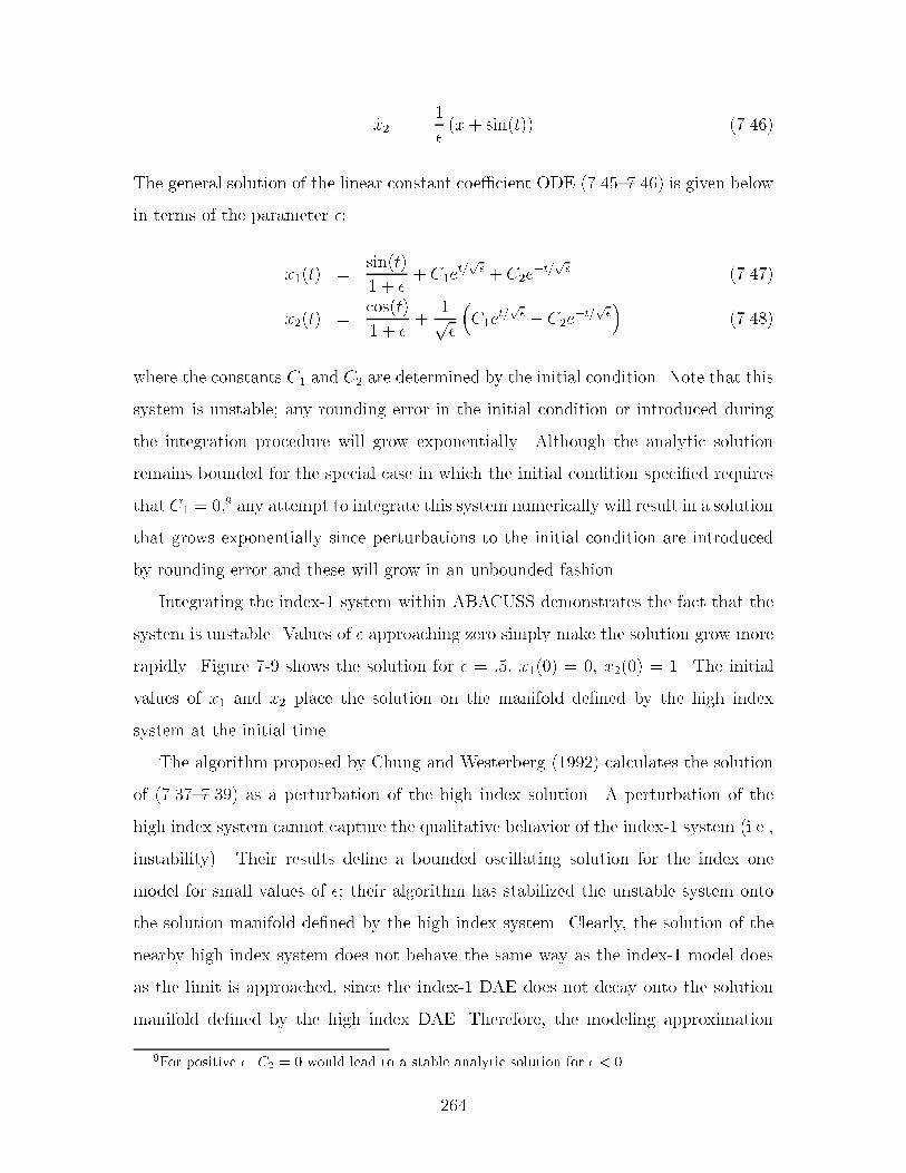
$x� ��
��x" sin�t�� �����
The general solution of the linear constant coe�cient ODE ��������� is given below
in terms of the parameter ��
x��t� �sin�t�
� " �" C�e
t�p " C�e
�t�p �����
x��t� �cos�t�
� " �"
�p�
�C�e
t�p � C�e
�t�p
�����
where the constants C� and C� are determined by the initial condition Note that this
system is unstable� any rounding error in the initial condition or introduced during
the integration procedure will grow exponentially Although the analytic solution
remains bounded for the special case in which the initial condition speci�ed requires
that C� � ��� any attempt to integrate this system numerically will result in a solution
that grows exponentially since perturbations to the initial condition are introduced
by rounding error and these will grow in an unbounded fashion
Integrating the index� system within ABACUSS demonstrates the fact that the
system is unstable Values of � approaching zero simply make the solution grow more
rapidly Figure �� shows the solution for � � ��� x���� � �� x���� � � The initial
values of x� and x� place the solution on the manifold de�ned by the high index
system at the initial time
The algorithm proposed by Chung and Westerberg ������ calculates the solution
of ��������� as a perturbation of the high index solution A perturbation of the
high index system cannot capture the qualitative behavior of the index� system �ie�
instability� Their results de�ne a bounded oscillating solution for the index one
model for small values of �� their algorithm has stabilized the unstable system onto
the solution manifold de�ned by the high index system Clearly� the solution of the
nearby high index system does not behave the same way as the index� model does
as the limit is approached� since the index� DAE does not decay onto the solution
manifold de�ned by the high index DAE Therefore� the modeling approximation
For positive �� C� � � would lead to a stable analytic solution for � ��
���

ABACUSS Dynamic Simulation
X1
X2
Y
Variable Values x 103
Time0.00
10.00
20.00
30.00
40.00
50.00
60.00
70.00
80.00
90.00
100.00
0.00 2.00 4.00 6.00 8.00
Figure ��� The unstable solution of the index� system
���
setting � � � is not valid and should not be made This example highlights the
danger of blindly transforming an index� system to the �nearby� high index system�
indicating that �near index� systems do not� in general� exist Some of the arguments
employed in the Chung and Westerberg paper ������ to demonstrate the existence of
near index systems were mathematically incorrect� so the authors were obviously led
to incorrect conclusions In addition� they applied their algorithm to several unstable
systems� but never mentioned or recognized that the systems were unstable However�
in some cases� such as those demonstrated in section ���� the behavior of the high
index system represents the limit of the index� DAE and the modeler may choose to
formulate the high index system to improve the solution e�ciency
�� Scaling Variables and Equations
Scaling the linear system solved at each corrector iteration o�ers the potential to
increase the accuracy of the solution obtained Typical scaling methods �reviewed in
section ���� employ two diagonal scaling matrices to transform the original system
����� into a scaled equivalent ����� The choice of scaling matrices encompasses
two issues� the condition of the scaled system and the validity of measuring the error
in the scaled system of variables If the condition number of the scaled system is
considerably smaller than the original� then we expect a more accurate answer in
terms of the transformed variables �y � D��� �x �Golub and Van Loan� �����
J�x � f �����
�D�JD���y � D�f �����
However� accuracy can only be improved if the scaling can be performed without
introducing any signi�cant error As long as the diagonal elements of the scaling
matrices are restricted to integer powers of the machine base� the transformation is
exact even if it is performed using �nite precision oating point arithmetic The
mantissas are not altered� so no rounding error is introduced �ANSI�IEEE Std ����
���

�����
Diagonal matrices that minimize the condition number of the scaled system exist
�Braatz and Morari� ������ yet their determination requires J��� so calculating them
is clearly not an option when our goal is to improve the accuracy of the solution to
����� in an e�cient manner We have implemented a scaling strategy to improve
the accuracy of �x� measured in the norm used by the integrator� at each corrector
iteration The strategy employs column scaling followed by row equilibration using
diagonal matrices composed of elements that are integer powers of the machine base
When the error is measured in the norm used by the integrator� this scaling policy
brings the condition number of the scaled system close to the minimum value that
can be achieved using any diagonal matrices This scaling policy improves the bounds
on the relative solution error The details of the row and column scaling algorithms
employed are justi�ed and explained in the following sections
���� Scaling the Variables
The way in which the error is measured dictates the choice of the matrix D� used to
scale the variables The matrix D� could be chosen to minimize the condition of the
column scaled equivalent JC � JD�� but as van der Sluis ������ has shown �JD��
may provide misleading information about the accuracy in the solution of ����� if
the way in which the error in �x is measured is important In fact� he states that
selecting D� to minimize �JD�� is similar to answering the question �in which norm
does the error look most favorable� �van der Sluis� ����� Since we would like the
condition number of the resulting system to be indicative of the quality of the solution
that will be obtained� we select D� to re ect our error criterion
The default norm used by the BDF integration routines to estimate the truncation
error and measure the size of the corrector updates was de�ned in ���� and has been
repeated here for convenience�
kxkBDF �
vuut �
n
nXi��
���� xi�ri jxpi j" �ai
�����
���

where xpi is the value of the variable xi from the previous integration step� �ri is the
relative error tolerance and �ai is the absolute error tolerance for variable i This
weighted root mean square norm is equivalent to �pn times the Euclidean norm
in the transformed system of coordinates� D��� �x� when D� is chosen according to
�����
D� � fD � Rn�n � dii � �ri jxpi j" �ai� dij � � � i �� jg �����
The condition number of the transformed matrix JC provides an indication of the
quality of the solution that can be expected from the solution of the linear sys
tem ����� in the absence of row scaling Let �x and �f represent the error in
f and �x respectively Assuming that the only error introduced during the cal
culation is due to the initial storage of f � then linear error analysis shows that
k�xk k�xk � �J� k�fk kfk However� the quality of the solution of ����� is
given by k�xkBDF k�xkBDF A bound on this quantity is provided by the same
linear error analysis applied to the transformed system shown in �����
JD�D��� �x � JC�y � f �����
k�xkBDFk�xkBDF
�k�yk�k�yk�
� ��JC�k�fk�kfk�
�����
Thus� when D� is selected according to ������ ��JC� is the condition number that
re ects the accuracy of the solution of the linear system
Scaling the variables in this way is easy to implement and has several advantages
It re ects the physics of the problem by using information that is available within the
integrator and passes this information to the linear algebra It permits the modeler to
work in a convenient set of units� greatly diminishing the need to select units for the
simulation variables merely to improve the performance of the numerical algorithms��
It automatically adapts when variables change over many orders of magnitude during
the course of the simulation� a common occurrence in batch process simulations
�The consistent initialization of such problems is not a�ected by this scaling and remains sensitiveto the units selected�
���

In addition� this scaling ensures that the magnitude of each of the elements of the
iteration matrix properly re ects the way in which the error of the linear system will
be measured� the selection of pivots during Gaussian elimination and the selection of
the scale factors used during row equilibration are governed by the magnitude of the
elements in the iteration matrix Since pivots are selected to reduce the growth in
the solution error and the row scaling factors are chosen to reduce the condition of
the linear system� choosing D� to re ect the way in which the integrator measures
the error should result in a more accurate solution of the linear system in terms of
the BDF norm Furthermore� the condition of the scaled iteration matrix can be
calculated using a Euclidean norm� this provides the condition of the original matrix
calculated according to the norm used by the integrator Therefore� the condition of
the scaled iteration matrix indicates the di�culty in obtaining an accurate solution in
terms of the way in which the integrator measures accuracy Using the scaled iteration
matrix JC � the accuracy criterion ����� derived in section �� can be applied using
the condition number de�ned on the two norm
To implement the scaling de�ned above as part of a numerical algorithm� D� is
approximated using integer powers of the machine base � This provides the matrix
%D� de�ned in ����� for a base two machine
%D� � fD � Rn�n � dii � �blog��rijxpi j�ai�c� dij � � � i �� jg �����
Only integer powers of the machine base need to be stored to de�ne the matrix These
can be calculated e�ciently using the functions recommended in the IEEE oating
point standard �ANSI�IEEE Std ���� �����
���� Scaling the Equations
The equations are scaled to minimize the condition number of the column scaled
iteration matrix The scaling employed balances the rows of JC � an integer scale
���

factor is chosen so that the scaled norm of each row is between one and �
D� � fD � Rn�n � dii � ��blog�kJikc� dij � � � i �� jg �����
In the rest of this section we will demonstrate that although this approach does not
guarantee a reduction of the condition of the matrix� for the sparse matrices in which
we are interested� it guarantees that the condition of the scaled matrix is close to the
condition of the optimally row scaled matrix We extend the results of van der Sluis
������ to prove that the scaling matrix de�ned in ����� provides a �scaled equivalent
of JC with a condition number that is within a factor of �pq of the optimally row
scaled matrix de�ned on the two norm� where q is the maximum number of nonzero
elements in any column of JC
Van der Sluis ������ generalized the work of Bauer ������� proving the row equili
bration theorem and demonstrating that row equilibration can satisfy the optimal row
scaling for a fairly wide class of norms However� row equilibration does not �nd the
optimal scaling matrix to minimize the condition number de�ned on the two norm�
which is the condition number of JC that re ects the fact that the error is measured
in the BDF norm We extend this work to show that simple row equilibration allows
us to determine a �scaled equivalent of the iteration matrix that is with a factor of
�pq of the optimal
Van der Sluis ������ used the row equilibration theorem �theorem ��� to show
that �� (DA� is within a factor ofpm of the optimally scaled matrix in terms of the
two norm We extend his result ����� to sparse matrices in the following corollary
Corollary � � Let (D be the scaling matrix that equilibrates the two norm of the rows
of (DA� The condition number of (DA de�ned on the two norm is within a factor ofpq of the condition number of the optimal row scaled matrix� so�
�� (DA�
minD�Dm ��DA�� pq �����
Proof� Given kAk� �pqmaxj
���AH�j����van der Sluis� ������ we obtain the follow
���

ing inequality
��� (DA����
�� (DA�� pq
maxj
����� (DA�H�j
����
�� (DA������
We employ the fact that �DA is row equilibrated and divide both sides of �����
k �DAk�
� �DA
minD�DmkDAk��DA
�pqk �DAHkk
�
� �DA
minD�DmkDAk��DA
� k � �� �� � � �m �����
Use ����� and ����� to substitute for the numerator on the right hand side of ������
k �DAk�
� �DA
minD�DmkDAk��DA
� pqminD�Dm
kDAk��DA
minD�DmkDAk��DA
� k � �� �� � � �m �����
which simpli�es to the desired result for the appropriate choice of ��
k �DAk�
� �DA
minD�DmkDAk��DA
� pq �����
Let ��A� � infx�Rn�kxk��� kAxk� kxk� � kA��k�
Rowequilibration �solves� the scaling problem for certain classes of norms and
bounds the distance to the optimal for ��DA� when optimizing over D � Dn How
ever� when using the matrix in a numerical algorithm� the scaling matrix must be se
lected from the space of diagonal matrices consisting of integer powers of the machine
base to eliminate the possibility of introducing roundo� error during the transfor
mation�� At �rst glance� this indicates that an integer programming problem must
be solved to �nd the optimal scaling matrix� but theorem �� demonstrates that a
solution with condition number that is within a factor � of the best obtainable can
be found easily
��An added bene�t is that functions usually exist ANSI IEEE Std� ���� � ��� to manipulatethe exponent of the �oating point number directly� allowing such manipulations to be performedextremely e�ciently�
���

Let %Dm be the class of nonsingular m�m diagonal matrices with nonzero elements
that are integer powers of the machine base � %dii � ��i where �i is any integer� The
following theorem proves that the optimal value of ��DB���DA� over %Dm is within
a factor of � of the optimum over Dm for any functions � and � satisfying the
assumptions of the row equilibration theorem
Theorem � � For A�B � Rm�n with ��DB� � maxj����DB�H�j
���� where k�k� is
an absolute norm� and ��DA� is left�monotonic on DmA� de�ne (D � Dm as the
matrix that minimizes ��DB���DA� over Dm� Let �i � �jlog � (dii�
kand de�ne %D
as an integer approximation to (D with elements %dii de�ned as follows
%dii �
��� ��i if ��i � (dii � ��i����
��i�� if ��i���� � (dii � ��i�������
The minimum of ��DB���DA� over %Dn is within a factor of � of the optimal over
Dm� so
minD�Dm
��DB�
��DA�� min
D� �Dm
��DB�
��DA�� � min
D�Dm��DB�
��DA������
Furthermore� rounding the nonzero elements of (D to an integer power of the machine
base according to ��� � de�nes the matrix %D � %Dm that satis�es ���� for all � such
that � � � � ����
�� %DB�
�� %DA�� � min
D�Dm��DB�
��DA������
Proof� Let -D�m and -D�
m be the classes of nonsingular m �m diagonal matrices with
nonzero elements satisfying -d�ii � ���� �' and -d�ii � &�� �� for i � � � � �m respectively
��The parameter allows the theorem to apply whether the elements of the diagonal scalingmatrix !D is rounded up or down to the nearest integer power of two�
���

De�ne -Dm � -D�m � -D�
m Since -Dkm%Dm � Dm for k � �� ��
minD�Dm
��DB�
��DA�� minDf� �Dkm�D�� �Dm
��DfD B�
��DfD A������
Using the facts that � is leftmonotonic and maxj����DB�T �j
���� mink jdkkjmaxj
���BT �j����
we have the following
minDf� �Dkm�D�� �Dm
��DfD B�
��DfD A�� min
Df� �Dkm�D�� �Dm
��DfD B�
maxj jdfjjj��D A������
� minD�� �Dm
mini jdfiij��D B�
maxj jdfjjj��D A������
� minD�� �Dm
�
�
��D B�
��D A������
The left hand inequality in ����� is self evident
To prove the second part of the theorem� de�ne -D � %D�� (D and use ����� to
show the following holds�
� � -dii � ���� if ��i � (dii � ��i����
��� � -dii � � if ��i���� � (dii � ��i�������
Therefore� -djj � ����� ����� for all j � �� � � �m Substitute %D -D for (D to show that
%D satis�es the same bound given for the optimal D � %Dm
minD�Dm
��DB�
��DA���� -D %DB�
�� -D %DA�� mini j -diij�� %DB�
maxj j -djjj�� %DA��
����� %DB�
������ %DA��
�
�
�� %DB�
�� %DA������
Theorem �� demonstrates that we can easily determine a row scaling that gen
erates a �scaled equivalent of A that is within a factor of � of the best possible
row scaled matrix for any condition number for which the row equilibration theorem
applies Moreover� if A � B � Rn�n and (D equilibrates the two norm of the rows
of A and ��A� � infx�Rn�kxk��� kAxk� kxk�� then combining the results of �����
and ����� demonstrates that �� %DA� is within a factor of �pq from the minimum
���
��DA� over D � Dn for the diagonal matrix %D de�ned in �����
��� %DA����
�� %DA�� pq
maxj
����� %DA�T �j
����
�� %DA�
� �pq minD�Dm
maxj����DA�T �j
���
��DA�� �
pq minD�Dm
kDAk���DA�
�����
Equation ����� shows that we can easily calculate a �scaled equivalent of the
scaled corrector iteration matrix JC � simply by equilibrating the two norm of the
rows of JC and rounding to an integer power of the machine base according to �����
Thus� we can scale the corrector iteration matrix by �rst scaling its columns� and
then scale its rows using the matrix %D The resulting matrix is within a factor �pq
of the optimally scaled matrix in terms of the way the integrator measures the error�
and it can be calculated e�ciently
The scaling algorithm that we have implemented within DASOLV and DSL��S
scales the iteration matrix every time it is reevaluated� typically after several integra
tion steps First the columns of the matrix are scaled� then the rows are scaled using
the %D de�ned in ����� when � � � However� the �i used to de�ne %D are determined
without actually calculating the two norms of the rows of JC to make the algorithm
more e�cient Let ji � �JTC�i The �i must satisfy the de�nition given in theorem ��
which can be rearranged as follows to eliminate the square root operation �proved in
theorem A���
�i � � �log �kjik��
�� �
jlog
��jTi ji
����k� �
�
�log
�jTi ji
�!�����
Since the rows of JC are sparse� the dot product jTi ji can be calculated e�ciently
�requiring O��n� operations��� The oor of log can be performed very e�ciently
by employing the logb function recommended by the IEEE oating point standard
�ANSI�IEEE Std ���� ����� which is de�ned as logb�x� ����log �x���� The func
��Du� et al� � ��� de�ne � as the number of nonzero entries in the matrix� so ��n is the averagenumber of nonzeroes per row�
���

tion merely accesses the exponent of the binary representation of the oating point
number The right hand side of ����� can be rewritten using the fact that bykc �bbyc kc for any integer k to make use of logb Thus� �i can be calculated according
to ������ the cost of this calculation is dominated by the computation of the dot
product of a sparse vector
�i �
�
�logb�jTi ji�
!�����
Only the vector � needs to be stored to represent the matrix %D The iteration matrix
may be scaled either implicitly �Forsythe and Moler� ����� during the calculation or
explicitly before it is factored using the function scalb �ANSI�IEEE Std ���� �����
Currently� we use explicit scaling to avoid making any changes to the sparse linear
algebra routines
The combination of row and column scaling just presented has reduced the con
dition number of the iteration matrix on all of the example problems on which it has
been tested In fact� scaling has reduced the condition number on the batch distil
lation models from approximately ���� to ��� Thus� the scaling method o�ers the
opportunity to extend the range of problems that may be solved with a machine of
given precision If the condition number of the corrector iteration matrix is reduced
substantially� the scaled iteration matrix may meet the conditions under which accu
racy may be guaranteed while the unscaled matrix cannot The scaling has entirely
eliminated the spikes observed on some simulations where the requested tolerance has
been loosened� and on other simulations the scaling has reduced the number of spikes
that have been observed The scaled simulation is solved more e�ciently because
there are fewer truncation error failures� residual evaluations� and Jacobian factoriza
tions However� in both cases the residual error combined with the condition of the
iteration matrix are not su�cient to guarantee the accuracy of the solution
An e�cient implementation of this scaling has been coded directly within the
DASOLV and DSL��S integrators and is transparent to the user�� The scaling algo
��The user merely sets a �ag to indicate that scaling should be performed� In ABACUSS� this
���

rithm can be applied to any BDF integration code on any machine that adheres to the
IEEE oating point standard� although it is most suited for sparse systems We have
already ported and tested the scaling on more than �ve Unix platforms Preliminary
results show improvements to the integrator�s e�ciency even on problems that can
be solved accurately with the standard integration scheme� these improvements are
more noticeable using DASOLV
�� Automatic Detection of Potential Inaccuracy
The criterion indicating an accurate solution of the corrector iteration ����� can be
checked after the solution of every corrector iteration In order to apply this criterion
the following quantities are required�
� A bound on the error in the residual values
� The condition number of the corrector iteration matrix� or an upper bound on
the condition number
� A bound on the backward error resulting from the LU factorization of the
corrector iteration matrix
In order to apply the criterion automatically� these quantities must be calculated e�
ciently so the checks can be performed without reducing the e�ciency of the numerical
integration code
A bound on the rounding error in the equation residuals can be calculated every
time the terms in the corrector iteration matrix are evaluated provided that the re
verse mode of automatic di�erentiation is employed �Iri et al�� ����� Iri and Kubota�
����� Kubota and Iri� ����� Since the reverse mode of automatic di�erentiation is
implemented within ABACUSS �Tolsma and Barton� ������ estimates of the residual
error �f are available In addition� the backward error resulting from the LU fac
torization of the iteration matrix can be determined during the factorization of the
matrix itself at little additional cost �Reid� ����� Arioli et al�� �����
option can be set at run time�
���

In general� estimating the condition number of a matrix is a di�cult task How
ever� since the matrix with which we are dealing is a sparse� rowequilibrated matrix�
fairly tight upper bounds on the condition number can be obtained For a row equi
librated matrix� a bound on the condition number is obtained from the determinant
of the row equilibrated matrix as follows �Guggenheimer et al�� ������
���DJ� �����det��DJ���� �����
Guggenheimer et al� ������ show that no tighter bound on the constant � is possible
From theorem ��� the condition number of the �equilibrated matrix� �� %DJ�� is
within a factor of � of the row equilibrated matrix� so
�� %DJ� ������det��DJ���� �����
The determinant of the row equilibrated matrix can be evaluated simply by multi
plying the pivots of the factored� row equilibrated matrix Unfortunately� the matrix
�DJ was not formed during the scaling process� instead� the �equilibrated matrix was
formed and factored However� the elements of �D were calculated before the matrix
was scaled in order to obtain �D Since �D � �D�D� the determinant of �DJ can be
calculated as long as the elements of �D are stored when �D is calculated In fact�
det��DJ� � det��DJ� det��D� �����
The determinant of �DJ can be determined by multiplying the pivots of the �
equilibrated iteration matrix� and the det��D� can be determined as the row scaling
factors are calculated For the scaling that has been implemented� � � -dii � �
The criterion ����� required that � � �� and we noted that if this was not
satis�ed� then ����� should be applied directly in order to estimate k�xkBDF We
now argue that we can bound the value of k�xkBDF from the information provided by
the evaluation and factorization of the corrector iteration matrix During evaluation
���

of the matrix we obtain an estimate for �f and during the factorization we obtain
an estimate of �J Our estimates for these quantities will not change during the
corrector iteration unless the matrix is reevaluated Newton�s method for the solution
of nonlinear systems is stable when started from within the region of convergence
�Wozniakowski� ������ so we consider the rounding error introduced if we had the
exact solution of the system Numerical evaluation of the function at the exact
solution x� di�ers from zero only by the error in evaluation the function �f �
f�x�� � �f " � �����
and from perturbation analysis of the system at x��
�J" �J���x " �x� � �f �����
Since we have assumed that x� is the exact solution to the f�x� � �� �x � � Using
the perturbed system ������ a result analogous to ����� obtained�
k�xkBDF � �J�
kJkBDF � �J� k�JkBDFk�fkBDF �����
Thus� every time the corrector iteration matrix is factored and evaluated we can
determine whether k�xkBDF � � indicating the possibility that the desired corrector
tolerance cannot be achieved even when the numerically calculated Newton update
is zero We note that we would like to converge the corrector iteration so that the
numerically calculated Newton updates are less than ���� k�xkBDF
��� E�ect of Scaling
The implemented scaling technique serves two purposes First it enables us to auto
matically scale models better than any user of the system could scale the models by
selecting appropriate units for the system variables� because a scale factor is selected
locally �in time� for each variable� rather than each type of variable �eg� enthalpy�
���

temperature� etc� Second� the scaling determines the optimal condition of the sys
tem for the purposes of error analysis� and enables us to bound the condition number
of the iteration matrix e�ciently
We recognize that the improvements to the performance of the code hinge upon
whether the scaling a�ects the selection of the pivots during Gaussian elimination
Since the matrix has been scaled by integer powers of the machine base� Gaussian
elimination will calculate exactly the same answer if the same pivots are selected
�Forsythe and Moler� ����� However� if the pivots change� then the answer may
change as well Therefore� the scaling helps the integration if it leads to better
pivot selection during the linear algebra The column scaling is required so that
the pivot selection is attempting to minimize the backward error in the appropriate
norm The row scaling can only help the performance if it reduces the backward
error of the matrix factorization However� many linear algebra packages decide to
row equilibrate matrices before attempting to factor them� so this is normally a good
procedure Since MA�� does not row equilibrate the matrix� this should help� but we
cannot guarantee that it will Since the backward error of the Gaussian elimination
grows with the system size� larger systems are more likely to cause problems when the
condition number is the same� and our scaling is more likely to bene�t these systems
The scaling also permits us to analyze the answers that we obtain from the Newton
iteration The accuracy of the Newton iteration is limited by the error in the residuals
and the condition number of the Jacobian The condition number that we should use
in these circumstances is the minimum condition number� so we would like to have
a wellscaled matrix Our scaling provides us with a reasonably tight bound on the
condition number that can be employed to detect systems in which the potential for
loss of accuracy exists
The scaling will have no e�ect on the performance of the integration code if the
same pivots are selected� so for systems that are well scaled over the entire time
domain the same performance can be expected Since the scaling is implemented very
e�ciently� it will not decrease the performance However� for poorly scaled systems�
the scaling will probably change the pivots that are selected and thus change the
���
performance of the code This is easily seen by noting that the choice of units in
which the model variables are expressed can cause simulations to fail The ability
to automatically detect the potential for inaccurate solutions due to illconditioning
allows the code to warn users of this possibility However� we should note that this is a
worst case scenario Note that the maximum magni�cation of the error in the solution
is rare� both the error and the residuals must be in the appropriate directions for this
to occur Therefore� on many illconditioned systems� the integrator may perform
quite well because the maximum ampli�cation of the error is not observed Our
examples merely demonstrate that in some cases the ampli�cation of the error does
occur
�� Conclusions
Equationbased simulation languages provide a exible environment in which to pose
dynamic simulation problems� yet this exibility puts severe demands on the embed
ded numerical solution algorithms We have found that the batch distillation of wide
boiling azeotropic mixtures is a very di�cult problem for the numerical integrator
used within ABACUSS In fact� we have discovered di�culties during the integra
tion of such problems that clearly indicate that the desired solution accuracy cannot
be achieved We have proven that that these problems stem from the inability to
obtain accurate solutions from the corrector iteration of the BDF integrator Using
linear error analysis� we have proven that the accuracy of the corrector depends on
both the condition of the iteration matrix and the accuracy to which the residuals
are evaluated We then proved that an illconditioned iteration matrix can lead to
the observed problems Furthermore� we have demonstrated that even nonsti� linear
time invariant ODE systems can become illconditioned
We have derived a criterion under which we can ensure that the desired accu
racy can be maintained and that the simulation results can be trusted For well
conditioned systems� the BDF methods should have no problem obtaining an accu
rate solution as long as the residuals are accurate However� the batch distillation
���
examples given here do not meet this criterion� and we admit the possibility of the
observed inaccurate solutions
Since wellconditioned systems can be solved reliably� we have investigated scal
ing techniques to improve the conditioning of the corrector iteration matrix Two
diagonal scaling matrices� with nonzero elements that are integer powers of the ma
chine base� are used to transform the linear system encountered at each corrector
step without introducing any rounding error We have shown that the column scaling
must be chosen to re ect the error criterion imposed by the BDF integrator Once
the columns have been scaled to re ect this error criterion� we are free to choose the
row scaling that minimizes the two norm condition number of the resulting system
Finding an exact minimizer of the two norm condition requires the solution of an
integer programming problem However� by extending the results of van der Sluis�
we have proven that for the sparse matrices in which we are interested� we can obtain
an approximate solution of this problem with a condition number that is quite close
to the minimum We have demonstrated that this approximate minimizer can be
determined without even evaluating the condition number of the system This scal
ing can be performed automatically and e�ciently within any BDF integrator We
have implemented the algorithm within both DASOLV and DSL��S the integration
codes used within ABACUSS The code is very e�cient� making use of functions that
manipulate the exponents of the binary representation of the oating point numbers�
and is entirely transparent to the user of the integration code
This numerical scaling technique has been shown to mitigate the problem of ill
conditioning on the distillation examples� reducing the condition number of the system
by �� orders of magnitude in some cases Unfortunately� problems can always be
constructed which are su�ciently illconditioned that the desired accuracy cannot be
guaranteed with a given machine precision In such cases� the simulation must be
performed in higher precision Note that these results apply to the dynamic simulation
of any system� not just batch distillation
Identifying potential problems in controlling the integration accuracy requires
bounding the condition of the iteration matrix� the error of the evaluated residu
���

als� and the backward error of the matrix factorization E�cient strategies for all are
required to identify and warn of potential problems automatically
Finally� the ability to make modeling decisions that improve the condition of
the DAE that is integrated has been illustrated Future development of these ideas
may focus on ways to interpret the information within the corrector iteration ma
trix to identify speci�c elements or sets of equations that may be leading to the
illconditioning of the matrix Proper identi�cation of the problematic terms may
permit the user to reformulate the model� if suitable modeling assumptions can be
made without sacri�cing the applicability of the results� in a way that enables the
numerical routines to perform better In addition� symbolic techniques capable of re
ducing the error in the calculated residuals may also increase the number of problems
that can be solved reliably� and these should be investigated further
���

Chapter �
Initial Step Size Selection for
DierentialAlgebraic Systems
�� Introduction
The transient behavior of many physical systems of interest exhibits both continuous
and discrete characteristics On the one hand� continuous behavior is naturally for
mulated mathematically as di�erentialalgebraic equations �DAEs� �Pantelides et al��
����� Brenan et al�� ����� Mattsson� ����� Cellier and Elmqvist� ������ and on the
other� discrete behavior is typically the result of either external control actions or au
tonomous discontinuities �Barton and Park� ����� Mathematically� discrete aspects
of the system behavior are modeled as changes in the functional form of the under
lying DAE The existence of such discontinuities complicates the solution procedure
and increases the need to start integration codes e�ciently
The solution of an initial value problem described by DAEs containing discon
tinuities can be formulated as a combined discrete�continuous simulation problem
�Cellier� ����� Barton and Pantelides� ����� In fact� the mathematical formulation
of this problem is typically represented as a sequence of initial value problems con
taining continuous models Discontinuities� commonly known as events� de�ne the
boundaries between these continuous domains and may result in a discrete change
to either the variable values� the functional form of the model� or both Thus� the
���

simulation domain of interest &to� tf� is partitioned into NC continuous subdomains
&tk��� tk� � k � � � � � NC in which to � t� and tf � tNC The combined simula
tion problem is de�ned as follows�
f k�xk� $xk� yk� uk� t� � �
uk � uk�t�
"#$ t � &tk��� tk� � k � � � � �NC ����
where xk � Rn�kx � yk � R
n�ky � uk � R
n�ku � and f k � Rn
�kx � R
n�kx � R
n�ky �
Rn�ku � R R
n�kx �n
�ky The event times tk may be de�ned either explicitly �time
events� or implicitly �state events� during the course of the simulation If all of the
discontinuities are de�ned explicitly� the solution of each of the initial value problems
may proceed in a straightforward fashion �Ellison� ����� Otherwise� the time at
which these events occur must be determined simultaneously with the solution of the
initial value problems� an e�cient algorithm for detecting and locating state events
within a linear multistep method has been developed by Park and Barton ������
In any case� the solution of a single combined simulation problem may require
the solution of many initial value problems Integration codes with the ability to
handle sti� systems� such as BDF methods� automatically adjust both the step size
and the order to produce an accurate solution e�ciently To maintain credibility
of the error estimates� which are based on the local error in the solution� the step
size control permits only moderate changes in the step length on any given step
Practical experience has shown that this strategy permits an e�cient solution once
the step size is �on scale� for the problem This implies that the step size chosen at the
beginning of each subdomain should be �on scale� for the current system dynamics
If the initial step is not chosen properly� the step size control is quite ine�cient at
�nding a value that is on scale Moreover� the error estimates may fail to recognize
an unacceptable solution when the step size is not on scale Since the integrator
will be started many times during a combined simulation experiment� the reliability
and e�ciency of the initial phase of the integration algorithm can have a signi�cant
impact on the performance of the overall solution procedure
���

This chapter derives an e�cient method to start the integration code for an ar
bitrary initial value problem in DAEs� corresponding to any particular instance �k�
in ���� Since this work has been motivated by combined simulation problems� the
method has been tailored for the calculation sequence encountered during the com
bined simulation of DAE models �Park and Barton� ����� and the information that
is readily available in combined simulation environments such as ABACUSS� and
gPROMS �Barton� ����� The method applies to DAE systems with index � � for
which a consistent initial condition is known
Next� we examine the heuristics commonly used to select the initial step length
within ODE and DAE codes� and examine methods that have been employed to
improve upon these heuristics for ODE codes We then consider how some of the
fundamental di�erences between DAEs and ODEs �Petzold� ����b� a�ect the initial
phase of the integration code For example� the information available at the start
of the integration and the form of the equations to be solved preclude the direct
extension of the ODE methods However� since the underlying problem is similar�
the same basic ideas used to increase e�ciency and reliability at the start of the
integration apply In particular� the method we propose addresses the di�erences that
exist in the speci�cation of initial conditions for DAE systems We exploit the facts
that a consistent initialization calculation must be performed before the integration
method is called� and that expressions for the partial derivatives of the equations are
now commonly available within combined simulation environments
�� Initial Step Size Selection
The initial step size that is selected must be �on scale� for the problem under con
sideration It should be small enough to capture the dynamics of interest within
the requested accuracy� yet it should not be so small that it signi�cantly a�ects the
e�ciency of the solution A number of authors have addressed the selection of initial
�ABACUSS Advanced Batch and Continuous Unsteady�State Simulator� Process Modeling Soft�ware� a derivative work of gPROMS Software� Copyright � � by the Imperial College of Science�Technology and Medicine�
���

step length in codes used to solve ordinary di�erential equations �Gear� ����a� Watts�
����� Gladwell et al�� ����� Shampine� ������ and a more complete description of the
previous work can be found there Here we address the heuristics for initial step size
selection contained within popular DAE codes
Several rules of thumb are commonly employed to select the initial step size in
codes designed to solve ordinary di�erential equations The simplest strategy is to
require the user to provide an initial step size Another technique seen in practice is
to calculate the length of the initial step as a ��xed� fraction of the length of the �rst
output interval These are two of the strategies implemented within DASSL �Petzold�
����a�� if the user does not supply a value� DASSL defaults to either a fraction of
initial output length or the inverse of the norm of the variable derivatives �Shampine
and Gordon� ������ whichever is smaller Allowing the user to specify the initial step
size permits educated users to exploit knowledge about the speci�c system they want
to solve� but most users will supply a somewhat arbitrary value because they may not
have a good idea of what an appropriate initial step length is On the other hand�
the length of the �rst output interval should provide some indication of the scale
of the problem However� as Watts ������ discusses� the user may not care about
the initial behavior of the solution� so the �rst output interval may not re ect the
initial dynamics of the problem Furthermore� this criterion does not even consider
the solution accuracy desired Using the norm of the variable derivatives is more
sensible� however� the time derivatives of the algebraic variables are not required to
specify a consistent set of initial conditions for the DAE� and for systems evolving
from a steady state the time derivatives are initially zero
To ensure accuracy during the initial step� Sedgwick ������ suggested starting
the integration at the smallest permissible step size given the machine precision
The integrator will then steadily increase the step size until it reaches a reasonable
value Since most codes do not permit the step size to change too rapidly� with
this approach many steps will probably be required before the step size levels o�
at a reasonable value For example� DASSL only permits the step size to increase
by a factor of two on any step where an increase in step size is desired� in order
���

to insure that the error estimates remain valid �Brenan et al�� ����� For linear
multistep methods� a doubling of the step size often requires refactorization of the
corrector iteration matrix Therefore� starting with too small a step size will incur
unnecessary computational costs �for a dramatic illustration of this� see the bouncing
ball example in section ��� In addition� the asymptotic error estimates may become
so contaminated with roundo� errors that they prevent the step size from increasing
as it should �Watts� ������ reducing the e�ciency of the integrator even further
This phenomenon is likely to be magni�ed when dealing with DAE systems� since the
condition number of the iteration matrix scales as ��h� for index� DAEs �Petzold�
����b�� implying that the accuracy of the solution to the linear system solved at each
corrector iteration is more sensitive to rounding errors when the step size is small
If an initial step that is too large is attempted� the user relies on the integrator
to reduce the step size until the error criterion is satis�ed Such a situation arises
when the initial step length is selected as a fraction of the initial output interval
and the user is not particularly interested in the initial behavior of the solution
Several problems may result from such an approach The asymptotic error estimates
may not be valid for the large step sizes attempted initially In such cases� the
predictor will not be close to the true solution and may cause the corrector iteration
to fail The step size is reduced and the procedure is repeated until the corrector
converges and the integration tolerance is satis�ed For linear multistep methods�
the heuristics typically require refactorization of the corrector iteration matrix after a
failed corrector iteration or a signi�cant step reduction� so successive step reductions
are ine�cient In addition� the possibility exists that the error criterion could be
satis�ed at a step size which is too large for the asymptotic error estimates to be
valid In such a case� some local phenomena may be missed entirely �Watts� �����
For example� the norm of the di�erence between the predicted and corrected solutions
may not be a unimodal function� this implies that a solution that satis�es the error
tolerances may exist for which the corrector polynomial does not accurately represent
the true solution over the initial interval Although this phenomenon is probably rare�
the initial step size selection procedure should avoid such situations
���

More sophisticated strategies to select the initial step size have been developed
These strategies are based on estimates of the norm of the variables� derivatives
�Shampine and Gordon� ������ the value of the local Lipschitz constants �Shampine�
����� for the system� or the norm of the higher order derivatives �Watts� ����� Glad
well et al�� ����� Shampine� ����� of the variables at the initial time These methods
are concerned with both stability and accuracy when selecting the initial step size�
but in most cases it is assumed that the equations will not be sti� at the initial
conditions Although these ideas are applicable to linear multistep methods� most of
this work has focused on the application of onestep methods to explicit systems of
ODEs An estimate of the behavior of the solution at the initial time is developed�
and this estimate is used to �nd an appropriate initial step size In most cases� these
methods rely on the existence of explicit expressions for $x in terms of x and t
In this work� we follow the basic idea of deriving an approximation for the behavior
of the solution at the initial condition� but the treatment of fully implicit DAE systems
���� requires a di�erent approach to derive estimates of the initial solution behavior
In the next section� we highlight the di�erences between the explicit ODE systems
addressed in the past and the DAEs with which we are concerned
�� Scope
This work addresses the initial phase of the integration of index� DAE systems in
implicit form using a linear multistep method The systems considered are those
de�ned in ���� corresponding to a particular instance �k� We determine an e�cient
step size to be used during the �rst integration step on which a �rst order linear
multistep method is employed Consistent initial values �see section ��� $x�to�� x�to��
and y�to� are supplied to the integration routine These values are the result of a
consistent initialization calculation performed before the integrator is called Kr+oner
et al� ������ have shown that failure to provide consistent initial conditions will result
in a myriad of problems including possible failure of the integrator on the �rst step
and inaccurate solution of the problem In addition� routines to evaluate the partial
���
derivatives of f � and the derivatives of the input functions� dudt� are supplied
We do not consider any of these requirements as serious limitations of our approach
because we envision the primary application for this technique to be integration codes
embedded within modern combined simulation environments Within such environ
ments the functional form of the model is explicitly available� so the partial derivatives
can be calculated automatically and e�ciently �Tolsma and Barton� ����� Since the
user can specify a DAE model of arbitrary index within these systems� we advocate
the calculation of the consistent initial condition as a separate phase of the solution
procedure� the structure of the model is analyzed in this phase of the calculation
First� the equations that de�ne a consistent initial condition are identi�ed and solved
�Pantelides� ����� Feehery and Barton� ����a� Next� if the system is high index� in
most practical cases an equivalent index� DAE can be derived automatically �Fee
hery and Barton� ����a� Hence� even in the high index case� it can be assumed
that an index� system will always be passed to the numerical integration code for
solution Previous researchers have determined conditions under which the solutions
of the reinitialization problems required at the junctions of the simulation domains
�t � tk� are de�ned unambiguously �Br+ull and Pallaske� ����� Br+ull and Pallaske�
����� Barton and Park� �����
BDF �Gear� ����� integration codes have been shown to be e�cient and highly
reliable for the solution of index� DAEs� so these are typically employed within
simulation environments It is possible to start these methods at a higher order by
using onestep methods� such as a fourth order RungeKutta method �Gear� ����a�
Gear� ����b� Brankin et al�� ����� However� these techniques are most applicable
when the system is not sti� and an explicit RK method can be employed The
applicability of implicit RK methods for the same purpose is questionable because a
set of p nonlinear systems of equations must be solved to start a pth order method
�Gear� ����b� In many situations� the systems are not sti� during the initial portion
of the integration because the fast transients in the system are excited and the step size
is chosen based on accuracy rather than stability requirements �Lambert� ������ but
this property is not guaranteed In a simulation environment we wish to emphasize
���

the reliability of the numerical solution� and to minimize the need for user intervention
in tuning the solution process Hence� to ensure stability� we employ a �rst order BDF
method which is Astable �Hairer and Wanner� ������ this also permits us to take
advantage of the order selection strategies within DASSL
Hybrid techniques employing an explicit RK method initially that switches to
a BDF scheme for stability �Keeping� ����� were not considered in order to retain
the guarantees for the detection of state events provided by the method of Park and
Barton ������ In cases where state events are guaranteed not to occur in the initial
phase of the integration these methods may be e�ective� but guarantees concerning
stability and state event location cannot be provided in general
�� Methodology
A higher order approximation of the behavior of the solution at the initial time
is employed to start the �rst order BDF method e�ciently This approximation
estimates the di�erence between the �rst order method and the true solution to
provide an estimate of the initial step size The estimate is then employed to advance
the solution over the initial integration step and to solve for the length of this step
simultaneously The method consists of the following steps�
� Determine the derivatives of the algebraic variables $yo at the initial time The
second derivatives of the di�erential variables +xo are also obtained
� Estimate the value for the initial step size
� Advance the simulation over the �rst integration step� calculating the initial
step size and the variable values simultaneously
The objectives of the �nal two steps in this procedure are similar to those of
Gladwell et al� ������ and Shampine ������� these employ the basic concept proposed
by Sedgwick ������ in a more e�cient fashion The procedure is implemented by
modifying the integrator�s behavior over the �rst integration step Our approach
���

di�ers from those employed for ODEs because we are dealing with fully implicit DAE
models� and we assume that the Jacobian will be available
The �rst step is required because the consistent initial condition for the index�
DAE passed to the integration code does not de�ne $y� on the other hand� for the
explicit ODE case� the time derivatives of all the variables are always available from
a function evaluation The bene�ts obtained by using this information for the �rst
order prediction are demonstrated in section �� The estimate of +x also derived
at this step provides a convenient way to estimate the initial step size �hest� at the
second stage of our procedure This contrasts with the initial estimates employed
for ODE codes in which only �rst derivative information is typically available at the
start Attempts to obtain more information by taking small steps are complicated
by the fact that while the truncation error is reduced as the step size decreases� the
relative contribution of rounding error is increased as the step size decreases
The last step in the procedure involves the solution of a nonlinear system of
equations to determine the optimal initial step size and the solution of the DAE at
this time simultaneously The availability of the Jacobian matrix and an estimate for
the optimal step size from the previous steps in our method enables this system of
equations to be solved using a modi�ed Newton iteration The solution of this system
of equations satis�es the DAE model and the criteria employed to de�ne the optimal
initial step size� which are described in section �� Note that these criteria consider
the step size and order selection heuristics employed by the integration code While
the examples provided within this paper employ the heuristics of the integration
code DASSL �Brenan et al�� ������ the same ideas apply to other linear multistep
methods At the conclusion of this step� we verify that the estimate of the local
truncation error decreases as the step size is reduced to support the assumption that
we have determined the �rst point at which the desired error norm is attained
The method outlined above exploits the fact that a consistent initialization calcu
lation has been performed in order to derive a linear system to calculate the algebraic
derivatives Although solution of this linear system is not required �a zero order
approximation for the algebraic variables could be employed in the predictor�� avail
���

ability of the derivatives of the algebraic variables enables much larger initial step
sizes to pass the truncation error tolerance In cases where any of the algebraic vari
ables are changing signi�cantly at the initial time� the zero order approximation will
not be very accurate This will result in a large di�erence between the predicted
and corrected solution on the initial integration step� requiring a very small initial
step in order to meet the error criterion Many additional steps are then required to
increase the step size to the value that might have been possible if these derivatives
were available In contrast� the algebraic derivatives can be determined with little
computational e�ort The bene�ts that this calculation has on the e�ciency of the
initial stages of the integration is demonstrated on a collection of example problems
detailed in section ��
The remainder of this chapter discusses each of the steps described above in more
detail First� the consistent initialization calculation is reviewed since the derivation
of the system employed in step � of our procedure relies upon the equations used to
determine the consistent initial condition This method is then compared with the
heuristics currently employed within DASSL� demonstrating the bene�ts of employing
this technique within combined simulation environments
� Consistent initial conditions
Before the integration of a system of DAEs can begin� a set of consistent initial con
ditions must be de�ned These are represented by initial values for the di�erential
variables x� their derivatives $x� and the algebraic variables y that satisfy the model
equations� their �rst and higher order time derivatives� and an additional set of speci
�cations enforced at the initial time The additional speci�cations take up the degrees
of freedom that remain when all constraints on $x� x� and y implied by the DAE model
and its time derivatives are taken into account The ability to express the initial con
ditions in terms of general algebraic relationships between the model variables at the
initial time� rather than simply specifying initial values for a subset of the variables� is
required to formulate many simulation problems of interest �Barton and Pantelides�
���

����� This work considers index� DAEs ���� for which the following matrix has
full rank�
��f
� $x
�f
�y
�����
When the matrix in ���� has full rank� the model equations ���� and additional
initial speci�cations ���� need to be solved simultaneously to determine initial values
$xo � $x�to�� xo � x�to�� and yo � y�to��
f� $xo� xo� yo� u�to�� to� � � ����
c� $xo� xo� yo� u�to�� to� � � ����
Therefore� c � Rnx �Rnx �Rny �Rnu �R Rnx We refer to the solution of �������
as a set of consistent initial conditions Note that full rank of the matrix shown in
���� is a su�cient condition for the index � �
The index one DAEs considered in this work represent models that are either
naturally expressed as index� di�erential algebraic systems� or that are a member of
the family of equivalent index� systems corresponding to a model that is naturally
expressed as a high index �ie� index � �� DAE The equivalent index� models con
sidered have been derived from the application of the dummy derivative algorithm
�Mattsson and S+oderlind� ������ which can be applied to high index models automat
ically �Feehery and Barton� ����a� This algorithm yields a DAE whose structural
index is one� for all such systems� the matrix appearing in ���� is structurally non
singular �Du� et al�� ����� The algorithm can also be applied to the class of special
index� DAEs �Pantelides� ����� that do not satisfy ���� based on structural crite
ria Thus� the implementation described here applies to all index� systems for which
structural criteria can correctly determine the additional equations constraining the
initial condition
Consistent initial conditions are obtained by solving f� $xo� xo� yo� uo� to� � � and
g� $xo� xo� yo� u�to�� to� � � Typically an initial guess that is close to the solution
���

is provided� either from a physical analysis or a solution obtained using another
numerical strategy such as homotopy continuation� and a modi�ed Newton method
is used to converge the system� we assume that an appropriate guess is provided� so the
method will succeed Implementation of this method requires the partial derivatives
of the f and g with respect to $x� x� and y These derivatives are easily calculated by
applying symbolic �Hearn� ����� or automatic di�erentiation techniques �Hillstrom�
����� Bischof et al�� ����� to the functions f and g� so they are readily available within
equation based modeling environments such as SpeedUp� ABACUSS� and gPROMS
�AspenTech� ����� Barton� �����
The convergence criterion speci�ed for the Newton iteration must take into ac
count the way in which error in the solution to the DAEs will be measured by the
integrator At the very least� the size of the �nal Newton updates for x and y must
satisfy the truncation error criterion employed on the �rst integration step to enable
the �rst integration step to proceed To ensure that the desired accuracy can be
achieved during the integration� the distance of the numerical approximation from
the exact solution to the initialization problem should be controlled� the impact that
the termination criterion has on accuracy of the numerical solution is discussed in
chapter � and elsewhere �Allgor and Barton� ����a� Iri� ����� Insu�ciently accu
rate convergence of the initialization problem will lead to the same type of numerical
di�culties caused by an inconsistent initial condition �Kr+oner et al�� �����
It is therefore assumed that the values of $xo� xo� and yo at the conclusion of
the Newton iteration provide su�ciently accurate consistent initial conditions for the
solution of the DAE model ���� Theoretically� no more information is required to
start the integration However� the integrator can be started more e�ciently if $yo is
provided The next section demonstrates that both $yo and +xo can be calculated quite
cheaply using a portion of the Jacobian matrix employed during the initialization
calculation
���
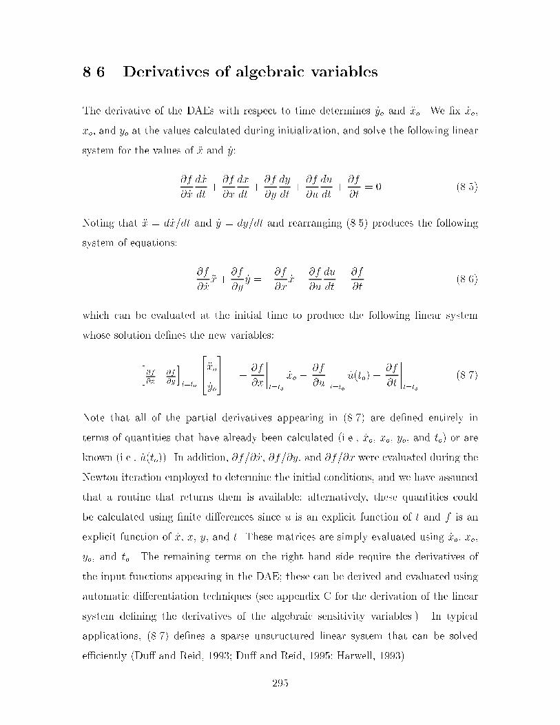
� Derivatives of algebraic variables
The derivative of the DAEs with respect to time determines $yo and +xo We �x $xo�
xo� and yo at the values calculated during initialization� and solve the following linear
system for the values of +x and $y�
�f
� $x
d $x
dt"�f
�x
dx
dt"�f
�y
dy
dt"�f
�u
du
dt"�f
�t� � ����
Noting that +x � d $xdt and $y � dydt and rearranging ���� produces the following
system of equations�
�f
� $x+x "
�f
�y$y � ��f
�x$x� �f
�u
du
dt� �f
�t����
which can be evaluated at the initial time to produce the following linear system
whose solution de�nes the new variables�
h�f� �x
�f�y
it�to
��+xo
$yo
� � � �f
�x
����t�to
$xo � �f
�u
����t�to
$u�to�� �f
�t
����t�to
����
Note that all of the partial derivatives appearing in ���� are de�ned entirely in
terms of quantities that have already been calculated �ie� $xo� xo� yo� and to� or are
known �ie� $u�to�� In addition� �f� $x� �f�y� and �f�x were evaluated during the
Newton iteration employed to determine the initial conditions� and we have assumed
that a routine that returns them is available� alternatively� these quantities could
be calculated using �nite di�erences since u is an explicit function of t and f is an
explicit function of $x� x� y� and t These matrices are simply evaluated using $xo� xo�
yo� and to The remaining terms on the right hand side require the derivatives of
the input functions appearing in the DAE� these can be derived and evaluated using
automatic di�erentiation techniques �see appendix C for the derivation of the linear
system de�ning the derivatives of the algebraic sensitivity variables� In typical
applications� ���� de�nes a sparse unstructured linear system that can be solved
e�ciently �Du� and Reid� ����� Du� and Reid� ����� Harwell� �����
���

To guarantee that ���� can be solved to determine unique +xo and $yo� the matrix
on the left hand side must be nonsingular During the consistent initialization� we
can check that the matrix shown in ���� is structurally nonsingular �Du� et al�� �����
�deriving an equivalent index� system for which this holds by applying the method
of dummy derivatives� if necessary� Thus� for any DAE system to which we have
obtained a consistent set of initial conditions for the equivalent index� model� we
will have a structurally nonsingular matrix in ���� However� this matrix may still
be singular� so we need to check the pivots of this factored matrix as we attempt to
solve this system Singularity of this matrix is not su�cient to show that ���� is even
locally index � �� but it raises the suspicion that the index of the system and�or the
degrees of freedom for consistent initialization cannot be properly determined using
structural criteria In these situations� the code terminates with a warning indicating
the strong suspicion that the model is still high index despite any attempts at index
reduction For example� consider the following linear constant coe�cient DAE�
$x� � x� " x� � y� � � ����
$x� � x� � x� " y� � � ����
x� " x� � � �����
The combination of Pantelides� algorithm and the method of dummy derivatives will
yield the following system�
$x� � x� " y� � y� � � �����
y� � x� � y� " y� � � �����
x� " y� � � �����
$x� " y� � � �����
where x� and $x� have been replaced by the algebraic variables y� and y� The matrix
���

&�f� $x �f�y' is given by�
�%%%%%%�
� �� � �
� � �� �
� � � �
� � � �
&&&&&&�
which� while structurally nonsingular� is still singular In the linear time invariant
case� this indicates that the structural algorithm has underestimated the true index of
this DAE� which is � Unfortunately� in general� no conclusions can be drawn about
the index of general nonlinear DAE systems based on the singularity of this matrix�
but we can suspect that the index has been underestimated
Factorizing the matrix on the left hand side of ���� dominates the computational
cost of determining +xo and $yo Since this matrix is smaller than the Jacobian matrix
used in the Newton iteration during initialization� the additional cost of calculating $yo
and +xo is expected to be small compared to the e�ort required to solve the initialization
problem
�� Initial step size
The integration will start using a �rst order method� so the initial step length can be
determined based on accuracy requirements alone� since the �rst order BDF method
is stable We consider the accuracy criteria when choosing the initial step size In
particular� larger steps will lead to a more e�cient solution if the accuracy can be
maintained using larger step sizes
The heuristics used to control the step size within DASSL adjust the step size
based on the estimate of the local error These error estimates are asymptotically
correct in the case of constant step size and order �Brenan et al�� ������ so the
heuristics within DASSL favor sequences of steps at constant size and order We
employ the following criteria to identify a step size to use on the initial step that will
lead to an e�cient integration�
���

� The initial step must satisfy the requested error tolerances
� The length of the second integration step must be the same size or greater than
the length of the initial step
� The norm used to measure local error in the solution must accurately represent
the deviation from the predicted solution� ie� the �rst order approximation
should interpolate the solution to within the requested tolerances over the do
main of the initial step
These criteria warrant some explanation The requested error tolerances are enforced
using the weighted norm of the di�erence between the predicted and corrected solu
tion Based solely on this criterion� the maximum step that satis�es the local error
criterion would be selected
The second criterion limits the size of the initial step in order to ensure that
the next step can be carried out at the same size The purpose of this criterion is
to take advantage of the heuristics employed within multistep methods that favor
sequences of steps of constant length and order The initial step size considers the
heuristic used to determine the length of the subsequent step For example� DASSL
employs a conservative strategy to select the size of the next step in order to limit
the number of truncation error failures� therefore� a fairly aggressive initial step can
pass the convergence tolerance� but the size of the succeeding step will be reduced In
addition� successive steps of the same size are typically required to increase the order of
the integration method DASSL only considers increasing the order of approximation
of a kth order method after k " � successful steps of the same length at order k
We assume that the potential bene�ts a�orded by increasing the integration order
outweigh any advantage that may be obtained by taking a slightly larger initial step
Since the second step will also employ a �rst order approximation� we will see that the
conservative step size heuristics dictate that our second criterion is more restrictive
than our �rst
The third criterion is included to ensure that no local phenomena in which we
are interested are missed because the initial time discretization is too coarse The
���

�rst order approximation to the solution is asymptotically correct� but the initial step
size needs to be small enough so that the local estimate of the error represents the
divergence from this asymptotic limit Therefore� the �rst point in time at which the
local error reaches the value de�ned by the second criterion is desired Although we
cannot guarantee that some important phenomena have not been missed� we select
the initial step size in a way that attempts to ensure that the �rst order approximation
properly interpolates the solution over the initial step Over this region� we expect
the norm of the di�erence between the predicted and corrected solution to increase
with step size� and we can easily evaluate the derivative of the error norm with
respect to step size at the completion of the initial step However� ensuring that
important phenomena are not overlooked is di�cult� because the numerical accuracy
of the solution to the model equations tends to decrease as the step size is decreased
because the corrector matrix becomes more illconditioned as h approaches zero for
index� DAEs
We refer to a step of maximum length that meets these criteria as the optimal
initial step size hopt in the remainder of this chapter� note that our de�nition di�ers
slightly from the de�nition of hopt used by Gladwell ������ and Watts ������ due to
the introduction of the second and third criteria Equations that de�ne hopt according
to the �rst two criteria are derived in the following section We demonstrate that these
equations can be solved during the �rst integration step by augmenting the system
of equations solved during the corrector iteration
����� De�ning the optimal initial step size
Although the consistent initialization calculations distinguish between the di�erential
and algebraic variables of the model� the integration code makes no such distinction
For convenience� the model equations are de�ned in terms of a single vector of vari
ables throughout the remainder of the paper Let nz � nx " ny� zT � &xT yT '� and
$zT � & $xT $yT ' Rather than de�ning a new function� we let the function f operate on
the vectors z and $z with the assumption that f� $x� x� y� u� t� � f� $z� z� u� t� where by
the de�nition of a DAE� �f� $z is singular everywhere The �rst criterion de�ning
���
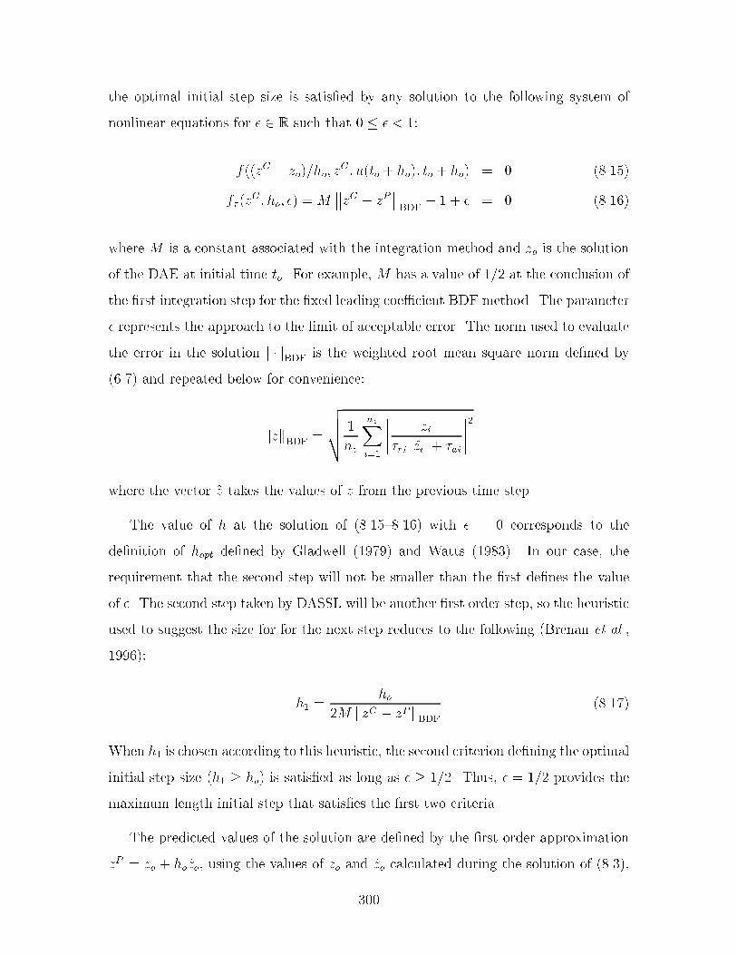
the optimal initial step size is satis�ed by any solution to the following system of
nonlinear equations for � � R such that � � � � ��
f��zC � zo�ho� zC � u�to " ho�� to " ho� � � �����
f �zC � ho� �� � M
��zC � zP��BDF
� � " � � � �����
where M is a constant associated with the integration method and zo is the solution
of the DAE at initial time to For example� M has a value of �� at the conclusion of
the �rst integration step for the �xed leading coe�cient BDF method The parameter
� represents the approach to the limit of acceptable error The norm used to evaluate
the error in the solution k�kBDF is the weighted root mean square norm de�ned by
���� and repeated below for convenience�
kzkBDF �
vuut �
nz
nzXi��
���� zi�ri j(zij" �ai
�����
where the vector (z takes the values of z from the previous time step
The value of h at the solution of ��������� with � � � corresponds to the
de�nition of hopt de�ned by Gladwell ������ and Watts ������ In our case� the
requirement that the second step will not be smaller than the �rst de�nes the value
of � The second step taken by DASSL will be another �rst order step� so the heuristic
used to suggest the size for for the next step reduces to the following �Brenan et al��
������
h� �ho
�M kzC � zPkBDF�����
When h� is chosen according to this heuristic� the second criterion de�ning the optimal
initial step size �h� � ho� is satis�ed as long as � � �� Thus� � � �� provides the
maximum length initial step that satis�es the �rst two criteria
The predicted values of the solution are de�ned by the �rst order approximation
zP � zo " ho $zo� using the values of zo and $zo calculated during the solution of �����
���

����� and ���� Equations ��������� are then solved for zC and ho using a modi�ed
Newton method that permits the use of a deferred Jacobian Initial guesses for zC
and ho must be provided in order for the method to converge A method to estimate
an initial guess for h is discussed in the next section This estimate seeks to �nd the
smallest value of h for which ��������� hold in order to satisfy the third criterion
above
����� Initial step size estimator
Any solution of ��������� satis�es the �rst two criteria for hopt provided � cor
responds to the step size heuristics of the particular code We also desire a value
ho for which the error estimate is also valid� noting that the values of ho satisfying
��������� may not be unique
For small ho� the di�erence between the solution predicted by the linear approxi
mation at to and the exact solution of the DAE is given by the higher order terms in
a Taylor series expansion about the initial point�
z�to " ho�� �zo " h $zo� � z�to " ho�� zP �h�
�+zo "O�h�� �����
The BDF method approximates the exact solution z�to"ho� with the solution of �����
zC The integration code maintains the validity of the approximation by controlling
the local truncation error� so the calculated solution zC obeys a similar relationship�
zC � �zo " h $zo� � zC � zP � h�
�+zo "O�h�� �����
From ������ we estimate the quantity zC � zP used to de�ne the local truncation
error in ����� using h�+zo� Using this approximation� an estimate of the initial step
size that satis�es ����� is given as follows�
hest �
s� ��� ��
M k+zokBDF�����
���

The error estimate is credible if the second term in the Taylor series dominates the
higher order terms in the series over a step of length hest The algebraic derivative
calculation provides +xo� but +yo is required to de�ne +zo completely Since only the norm
of +zo is required to estimate the initial step size and k�kBDF scales with the square
root of the number of elements in the vector� we assume that k +zokBDF � k +xokBDF as
an initial approximation At the conclusion of the initial integration step� we attempt
to verify that the di�erence between the predicted value and the solution zC at hest
for the di�erential variables is approximated by the second order term in the Taylor
series indicating that the contributions from the higher order terms are negligible
����� Initial time step combined with step size selection
The variable values and the optimal size for the initial step are simultaneously deter
mined during the �rst integration step The nonlinear system ��������� is solved
for &z�ho�� ho'T using a modi�ed Newton iteration in which a deferred Jacobian is
employed
The linear system solved at each step of the standard corrector iteration �ie� if
ho were speci�ed� on the initial integration step follows�
h�f�z
" �ho
�f� �z
i h�zk
i� G�zk � �f��zk � zo�ho� z
k� u� ho� �����
In order to solve for both z�ho� and ho simultaneously� we solve the following system
at each step of the Newton iteration�
���f�z
" �ho
�f� �z
� zk�zoh�
�f� �z
" �f�u
�u�t
" �f�t
�f��z
�f��h
����zk�hk
� � J
���xk�hk
� �
���f��zk � zo�h� z
k� u� hk�
�f �zk� hk� ��
�
�����
Observe that the standard corrector iteration matrix G is equivalent to the �rst nz
rows and columns of the Jacobian matrix J used for the modi�ed corrector iteration
On large problems� factoring the corrector iteration matrix dominates the compu
tational cost of the integration method� so BDF codes avoid factoring the corrector
���

iteration matrix at each time step by employing the already factored corrector itera
tion matrix from a previous time step until the convergence of the Newton iteration
deteriorates to an unacceptable level This implies that as long as the guess for hest is
reasonably close� the same Jacobian matrix can be used throughout the entire New
ton iteration� and that only the matrix G should be factored� so it can be used on
the subsequent integration step without requiring a refactorization
For the type of systems in which we are interested� the matrix G is sparse and
unstructured� so the integration code employs linear algebra routines that take ad
vantage of this �Du� and Reid� ����� Du� and Reid� ����� Although the additional
row contained in J is dense� the matrix J remains sparse The structure of J is ex
ploited by factoring only the matrix G and by treating the last row and column of J
separately At each Newton iteration ����� can be solved for the cost of two backsub
stitutions on a system of size nz and a couple of dot products� the solution procedure
is described in appendix B The main reason to avoid forming and factoring J is to
avoid having to refactor the corrector matrix on the next integration step However�
some additional bene�ts are obtained by exploiting the fact that the additional row
contained in J is dense The dense row in J removes any block diagonal structure
from J that may have existed in G Treating the additional row separately takes full
advantage the block structure of G� which is particularly important for the simulta
neous integration of a DAE system and its parametric sensitivities� for these systems�
e�cient solution techniques have been developed that exploit the fact that the linear
systems encountered will block decompose �Maly and Petzold� ����� Feehery et al��
�����
The derivative expressions appearing in the last column of J were required to
compute the derivatives of the algebraic variables in section ��� so routines to provide
them are assumed Let D de�ne the diagonal matrix of variable weights for the root
mean square norm�
D � Rnz�nz � dij �
�'�'�
�
jzoijri�ai if i � j�
� if i �� j
�����
���

The derivatives of f are expressed below in terms of the diagonal matrix D
�f�z
�M
nz kz � zP kBDFD�&z � zP ' �����
�f�h
��M
nz kz � zP kBDF&z � zP 'D� $zo �����
All the information needed to evaluate these terms is available at each step in the
iteration The denominators de�ned in ��������� are guaranteed to be nonzero at
the solution of the system because��z � zP
��BDF
� �� � ��M This ensures that
the last row of J is nonzero at the solution Another advantage obtained when the
additional row and column are excluded from the factored portion of the Jacobian
matrix is that the elements of these vectors can be updated at every step of the
modi�ed Newton iteration
Initial guesses for z�hest� are provided from the second order Taylor series evalu
ated at hest If the iteration fails to converge� the solution of the system is attempted
again at ��hest After two failures� we revert to a standard corrector iteration until a
feasible� not optimal� step size is determined
After successful completion of the integration step� we verify that the interpolation
of the calculated solution satis�es the BDF approximation of the model equations
We select a time h � hopt� such that h is not so small that it requires refactorization
of the corrector iteration matrix We check that the truncation error at this step size
is smaller While this does not guarantee that we have determined the smallest value
of h that satis�es ������ it veri�es that the �rst interpolated solution approximates
the computed solution of the BDF approximation of the model equations ����� at
the selected time
The iteration matrix G employed during the modi�ed Newton iteration is refac
tored according to the same heuristics used to decide whether to reevaluate the cor
rector iteration matrix in response to a step size change Therefore� the method
proposed will obtain the desired initial step size in the same number or fewer matrix
factorizations than would be achieved by simply starting the integrator with the ini
tial guess provided by our estimator� as long as the initial guess hest is close enough
���

to hopt to permit the Newton iteration to converge If hest is slightly larger than hopt�
we obtain the advantage that the second integration step can be taken at the same
step size by calculating hopt If hest is slightly smaller than hopt� a larger step can
be employed Since superlinear convergence of the corrector is achieved� the optimal
initial step size is determined with little additional e�ort The performance of the
method is discussed in section ��
� Implementation within DSL� S
The algorithm described in the preceding sections has been implemented within the
DAE code DSL��S �Feehery et al�� ����� � a code derived from DASSL �Petzold�
����a� that has been designed for large unstructured sparse systems of DAEs� em
ploying the MA�� �Harwell� ����� linear algebra routines The code automatically
scales the corrector iteration matrix to re ect the error norm employed and minimize
the condition number of the resulting corrector iteration matrix �Allgor and Barton�
����a� In addition� DSL��S employs an e�cient method for the integration of the
DAE with its associated sensitivity equations The code either uses a usersupplied
routine to evaluate the vector uodudt " �f�t required by the algebraic derivative
calculation or it determines these using �nite di�erences If sensitivity equations are
integrated as well� then DSL��S either employs the usersupplied routine that pro
vides ��f� $x�t � $x�p"��f�y�t �y�p"��f�p�t evaluated at to to determine the
derivatives of the algebraic sensitivities� or it determines them using �nite di�erences
All of the other information required to implement the algorithm is readily available
within the previous implementation of the code as since the Jacobian is required for
integration �DSL��S permits the use of a mixed analytic and numerical Jacobian�
A robust and e�cient implementation of the method described in the previous
sections requires that certain �special� cases are identi�ed and dealt with appropriately
First� the value for hest must be provided in cases when k+zokBDF � � Two cases are
considered depending on whether k $zokBDF � � If k $zokBDF �� �� then the following
���

estimate developed by Shampine ������ is employed�
hest ���� ��
� k $zkBDF�����
On the other hand� if k $zokBDF � �� then the code defaults to a fraction of the requested
initial output length The di�culty with the implementation of this scheme is to
determine when the norms are close enough to zero to be considered zero We check
to see whether k $zokBDF tout kzokBDF is small in order to relate the norm to the scale
of the problem Although this scheme may take a conservative initial step size in the
case when the system is sitting at steady state� or when only the second derivatives
are zero� we feel it is better to take a conservative approach rather than attempt to
take the maximum size step that the code will allow Recognize that if the system is
truly operating at steady state� then the augmented system of equations will not have
a solution because ����� cannot be solved since the prediction is the exact solution
of the system
The e�ciency of the iteration is a�ected by the criteria that are used to determine
whether the augmented system of equations ��������� is converged Obviously� the
convergence of the variables zC of the DAE must adhere to the same criteria used
for a typical integration step Since this criteria is based on the size of the updates
to the variable values� it will be di�cult to satisfy this criteria unless the step size is
no longer changing by an appreciable amount However a slightly smaller initial step
size� one that leads to a negative residual in ������ is acceptable if the magnitude of
the negative residual is close enough to zero� this is analogous to choosing a value of
� that is slightly larger than �� These facts indicate that e�ciency advantages may
be obtained by �xing the step size and merely converging the variable values once
����� obtains a negative value close enough to zero In general� such a strategy is not
appropriate to implement within Newton�s method because updates for all variables
are determined However� since ����� is the last equation in the system and ho is
the last variable� the update to ho can be set to zero before the back substitution on
the rest of the matrix is performed This is particularly easy to implement in our
���

augmented system since the last row and column are treated separately As shown in
appendix B� the updates to the variables in the absence of a change in ho are given
by v� The other advantage to this strategy is that the derivatives of f with respect
to both zC and h often contain signi�cant contributions from numerical error in the
evaluation of zC � zP which means that the step size may continue to change by
small amounts even when its value has essentially converged By �xing the step size
once it is near the answer� these small changes to the step size �possibly caused by
numerical error in the derivative expressions� cannot deteriorate the convergence rate
of the DAE variables
The Newton iteration has been modi�ed slightly to improve the convergence when
hest is a poor initial guess for hopt First� every time h is changed by a substantial
factor� or on the initial Newton step� only the DAE variables are updated in order
to get a more accurate value for f and to be able to evaluate the derivatives of
f This is a tailored recovery strategy from the guaranteed numerical singularity of
the Jacobian on the �rst Newton step that occurs because zP � zC�� This allows
the Newton step to update the values of the DAE variables on the �rst step and
determine the convergence rate of the Newton iteration Furthermore� large changes
to h are not permitted on a given Newton step� h is not permitted to change by more
than an order of magnitude on any given step If such a large change is indicated�
h is changed by an order of magnitude� and the variable values z are determined by
the predictor polynomial for a step of this length This strategy has improved the
convergence of the method in situations where hest provides a poor estimate for hopt
On most problems� the largest initial step length that will satisfy the error criteria is
desired because the relative size of the contributions of the numerical rounding error
to the variable updates will be smaller Since the error in the approximation of the
derivatives is being controlled by the truncation error criterion� the largest step that
satis�es the truncation error check should approximate the derivatives to the desired
accuracy
Finally� cases in which the addition of ����� to the DAE system leads to a singular
system must be handled These cases arise whenever zC � zP � �� so the last row
���

of the matrix becomes zero Since this always happens on the �rst Newton step�
the tailored recovery strategy mentioned above is employed However� singularity
of this matrix may occur on other steps as well Whenever the pivot corresponding
to h becomes too small� h is doubled �in an attempt to avoid situations where the
predictor is extremely accurate�� and a standard integration step is attempted at this
step length
���

�� Computational Performance
The computational performance of the algorithm is reported for a set of hybrid dis
crete�continuous simulation problems These examples show the bene�ts of this tech
nique in terms of both an increase in the initial step length and a reduction in the
number of Jacobian factorizations and residual evaluations that are required for the
overall simulation
First� the technique is demonstrated for a classic discrete�continuous simulation�
the bouncing ball When the ball is falling� the equations of motion in a gravity �eld
govern its trajectory� these equations de�ne a system of ordinary di�erential equa
tions When the ball hits the ground� the ball rebounds with a fraction of the vertical
speed at which it contacted the ground according to the coe�cient of restitution The
method of Park and Barton ������ that is used to locate discontinuities during the
simulation introduces algebraic variables and equations to the model that represent
discontinuity functions In the case of the bouncing ball� two discontinuity functions
are added to the model to identify when the ball hits the ground The �rst indicates
whether the ball is touching the ground �the center of the ball with diameter �m is
touching if y � ����� the second ensures that vy � � �ie� the ball is falling� The
equations representing the index � DAE model of the system are�
f �
�%%%%%%%%%%%%�
$x� vx
$y � vy
$vx
$vy " ����
d� " y � ���
d� " vy
&&&&&&&&&&&&�
� � �����
where x and y represent the position of the center of the ball� and vx and vy represent
the velocities in each coordinate direction Initial conditions of vx � �� vy � �� x � ��
y � ��� are speci�ed
This example demonstrates the advantage of determining the derivatives of the al
���
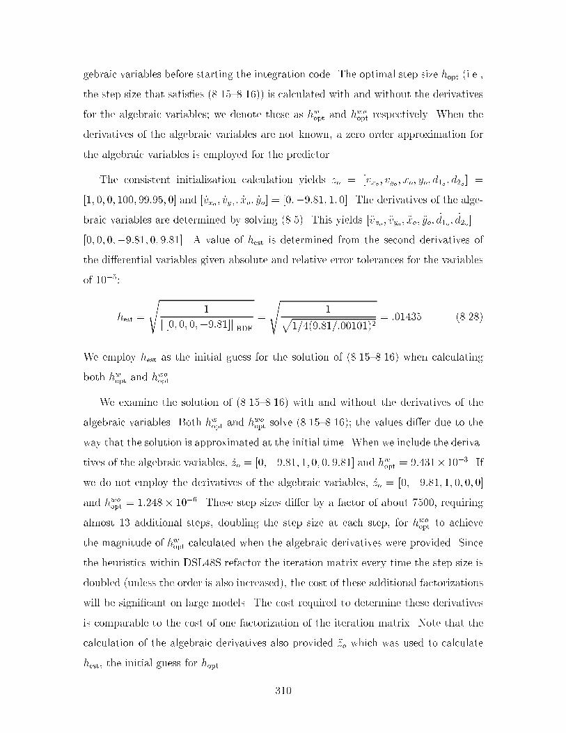
gebraic variables before starting the integration code The optimal step size hopt �ie�
the step size that satis�es ���������� is calculated with and without the derivatives
for the algebraic variables� we denote these as hwopt and hwoopt respectively When the
derivatives of the algebraic variables are not known� a zero order approximation for
the algebraic variables is employed for the predictor
The consistent initialization calculation yields zo � &vxo� vyo� xo� yo� d�o� d�o' �
&�� �� �� ���� ������ �' and & $vxo� $vyo� $xo� $yo' � &�������� �� �' The derivatives of the alge
braic variables are determined by solving ���� This yields &+vxo� +vyo� +xo� +yo� $d�o� $d�o' �
&�� �� �������� �� ����' A value of hest is determined from the second derivatives of
the di�erential variables given absolute and relative error tolerances for the variables
of �����
hest �
s�
k&�� �� �������'kBDF�
s�p
���������������� ������ �����
We employ hest as the initial guess for the solution of ��������� when calculating
both hwopt and hwoopt
We examine the solution of ��������� with and without the derivatives of the
algebraic variables Both hwopt and hwoopt solve ���������� the values di�er due to the
way that the solution is approximated at the initial time When we include the deriva
tives of the algebraic variables� $zo � &�������� �� �� �� ����' and hwopt � ���������� If
we do not employ the derivatives of the algebraic variables� $zo � &�������� �� �� �� �'
and hwoopt � ������ ��� These step sizes di�er by a factor of about ����� requiring
almost �� additional steps� doubling the step size at each step� for hwoopt to achieve
the magnitude of hwopt calculated when the algebraic derivatives were provided Since
the heuristics within DSL��S refactor the iteration matrix every time the step size is
doubled �unless the order is also increased�� the cost of these additional factorizations
will be signi�cant on large models The cost required to determine these derivatives
is comparable to the cost of one factorization of the iteration matrix Note that the
calculation of the algebraic derivatives also provided +zo which was used to calculate
hest� the initial guess for hopt
���
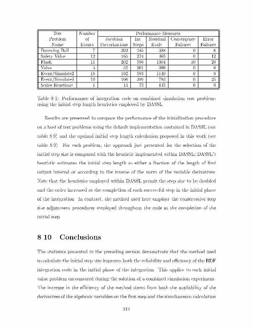
Test Number Performance MeasuresProblem of Jacobian Int� Residual Convergence ErrorName Events Factorizations Steps Evals� Failures Failures
Bouncing Ball � ��� ��� ��� �
Safety Valve �� � � ��� � � � ��
Flash �� ��� �� ���� �� ��
Valve � �� ��� �� �
Event�Simulate� �� ��� ��� ���� � �
Event�Simulate� �� � �� ��� � ��
Series Reactions � �� �� ��� � �
Table ��� Performance of integration code on combined simulation test problemsusing the initial step length heuristics employed by DASSL
Results are presented to compare the performance of the initialization procedure
on a host of test problems using the default implementation contained in DASSL �see
table ��� and the optimal initial step length calculation proposed in this work �see
table ��� For each problem� the approach just presented for the selection of the
initial step size is compared with the heuristic implemented within DASSL� DASSL�s
heuristic estimates the initial step length as either a fraction of the length of �rst
output interval or according to the inverse of the norm of the variable derivatives
Note that the heuristics employed within DASSL permit the step size to be doubled
and the order increased at the completion of each successful step in the initial phase
of the integration In contrast� the method used here employs the conservative step
size adjustment procedures employed throughout the code at the completion of the
initial step
��� Conclusions
The statistics presented in the preceding section demonstrate that the method used
to calculate the initial step size improves both the reliability and e�ciency of the BDF
integration code in the initial phase of the integration This applies to each initial
value problem encountered during the solution of a combined simulation experiment
The increase in the e�ciency of the method stems from both the availability of the
derivatives of the algebraic variables on the �rst step and the simultaneous calculation
���

Test Number Performance MeasuresProblem of Jacobian Int� Residual Convergence ErrorName Events Factorizations Steps Evals� Failures Failures
Bouncing Ball � �� � � ��� � �
Safety Valve �� ��� ��� ��� � �
Flash �� ��� �� ���� � ��
Valve � �� ��� ��� � ��
Event�Simulate� �� �� ��� ��� � �
Event�Simulate� �� ��� ��� ��� � ��
Series Reactions � � � ��� � �
Table ��� Performance of integration code on combined simulation test problemsusing the optimal initial step length calculation
of the variable values and the initial step length during the �rst integration step
Using the derivatives of the algebraic variables at the initial time improves the
accuracy of the prediction during the �rst integration step Without these deriva
tives the initial step length will be restricted to much smaller values In fact� if
the �rst order terms in the Taylor series for the algebraic variables dominate the
higher order terms� then the initial step size cannot be greater than the point at
which the norm of the �rst order terms exceeds the allowable error tolerance �ie�
(ho � �ny " nx�M�ny k $ykBDF�� The value (ho approximates the largest step size that
could succeed on the initial step if the $yo are not determined Since the derivatives
of the algebraic variables can be calculated inexpensively� the bene�ts appear clear
Determining these values allows the size of the initial step length to be governed by
the second order terms in the Taylor series This additional calculation improves the
performance of the integration of DAEs� distinguishing this method from those ap
plied to ODEs In addition� the algebraic derivative calculation provides the second
derivatives of the di�erential variables +xo which can be used to estimate the length
of the optimal initial step length
The second derivatives of the di�erential variables provide information that can
be employed to estimate an initial step size that maintains the validity of the error
estimate but is on scale for the problem The method presented establishes criteria
that de�ne the optimal initial step length We have demonstrated that a step satisfy
���

ing these criteria can be found by augmenting the system of equations solved during
the corrector iteration The augmented system of equations can be solved using the
same corrector iteration matrix Whenever a good initial estimate of the optimal
step size is calculated by our estimation procedure� the optimal initial step size can
be determined without any additional factorizations of the corrector iteration matrix
The solution statistics for the example problems demonstrate the improvements of
the e�ciency of the solution procedure In addition� the step size selection procedure
employed during the initial phase of the integration is more conservative and leads to
fewer convergence and error test failures� yet it remains more e�cient
Since this method improves both the e�ciency and reliability of the code in the
initial phase of the integration� it can provide signi�cant bene�ts for the hybrid
discrete�continuous simulation of large models with frequent discontinuities The
method is ideally implemented within combined simulation environments where the
required derivative information is available
���

���

Chapter �
MixedInteger Dynamic
Optimization
This chapter presents some preliminary results on how the decomposition approach
for the batch process development problem introduced in chapter � extends to a more
general class of mixedinteger dynamic optimization problems We de�ne mixed�time�
invariant�integer dynamic optimization as the class of problems for which the decom
position strategy applies� and demonstrate that simple extensions of mixedinteger
nonlinear programming �MINLP� techniques are doomed to failure on this class of
problems On the other hand� our approach combines dynamic optimization with
insight based targeting techniques to decompose the optimization into subproblems
providing rigorous upper and lower bounds on the objective This approach has the
potential to eliminate total enumeration of the discrete space� assures termination in
a �nite number of iterations� and yields a rigorous bound on the distance between
the solution found and the global solution
��� Introduction
Many problems in process design and operation require the optimal selection of
quantities that vary over time When a mathematical model of the process is avail
able� these quantities may be calculated using dynamic optimization� in fact� several
���
researchers in the chemical engineering community have developed algorithms for
the optimization of largescale dynamic systems �Cuthrell and Biegler� ����� Vas
siliadis� ����� Feehery and Barton� ����a� However� many problems also contain
discrete quantities or decisions that cannot be described using purely continuous
dynamic models of the system The growing recognition of the importance of dis
crete�continuous �or hybrid� dynamic systems to the chemical industry has recently
motivated the development of appropriate simulators �Barton and Park� ����� Sim
ilarly� the optimization of hybrid dynamic systems cannot always be performed using
purely continuous formulations This motivates new algorithms capable of handling
classes of mixedinteger dynamic optimization �MIDO� problems
Recently� dynamic optimization of large scale continuous systems has been demon
strated �Charalambides et al�� ����b�� and dynamic optimization capabilities have
even been embedded in process simulators such as ABACUSS However� limited
progress has been made that addresses dynamic problems coupled with discrete deci
sions Charalambides et al� ������ formulate �batch process synthesis� as a multistage
mixedinteger dynamic optimization problem� but no solution procedures have been
reported Mohideen et al� ������ consider design and control in the presence of uncer
tainty� formulating the problem as a stochastic mixedinteger optimal control problem
This problem is transformed into a �nite dimensional MINLP through discretization
of the time domain with orthogonal collocation on �nite elements However� the
nonconvexities inherent in this problem are not discussed� so the application of tradi
tional MINLP algorithms to this problem is likely to reduce to an ad hoc improvement
strategy that may prune the optimal discrete alternative �Sahinidis and Grossmann�
����� Bagajewicz and Manousiouthakis� �����
In contrast� we present a decomposition approach to MIDO that is capable of
providing rigorous bounds on the global solution in spite of the nonconvexities inher
ent in the variational subproblems In addition� this decomposition is the �rst that
permits either collocation or numerical integration based strategies to be used for
the variational subproblems In the following sections� we formally de�ne the MIDO
algorithm and the class of problems it addresses Further� we demonstrate how the
���

required subproblems can be derived and solved on a relatively simple batch process
development example
��� Problem Scope
We consider the class of mixedinteger dynamic optimization problems that conform
to the following formulation�
minut�v�y�tf
�Xk
�k�xk�tfk�� uk�t
fk�� v� y� t
fk� "
Xk
Z tfk
t�k
Lk�xk�t�� uk�t�� v� y� t�dt
�����
Subject to�
fk�xk�t�� $xk�t�� uk�t�� v� y� t� � � � k� t � &t�k� tfk' ����
gk�xk�t�� $xk�t�� uk�t�� v� y� t� � � � k� t � &t�k� tfk' ����
h�v� y� t� � � ����
�kp�xk�tp�� $xk�tp�� uk�tp�� v� y� tp� � � � k� p � f�� npkg ����
where
xk � Xk Rnx uk � Uk � R
nuk �ku �
�k
Uk � U Rnu v � V R
nv y � Y � f�� �gny
fk � Xk � Rnxk � Uk � V � &�� �'ny � R R
nxk
gk � Xk � Rnxk � Uk � V � &�� �'ny � R R
ngk
h � V � &�� �'ny � R Rnh
�kp � Xk � Rnxk � Uk � V � &�� �'ny � R R
nkp
and xk�t� are the continuous variables describing the state of the dynamic system k�
uk�t� are continuous controls whose optimal time variations on the interval &t�k� tfk' are
required� v are continuous time invariant parameters whose optimal values are also
���
required� y are a special set of time invariant parameters that can only take binary
values� and tfk is a special continuous time invariant parameter known as the �nal
time of system k This formulation allows for nk dynamic models that are coupled
by the time invariant parameters v and y It is the presence of the binary time
invariant parameters y that distinguishes formulation ������� from other recent quite
general dynamic optimization formulations �Vassiliadis et al�� ����� We conjecture
the existence of a more general class of problems that also contain binary controls
�ie� functions whose time variation is restricted to take �� values� but will only
consider the class ������� Hence� to coin a term� ������� might be called a mixed
time invariant integer dynamic optimization
The constraints ������� warrant some explanation Equations ���� represent
a general set of di�erentialalgebraic equations �DAEs� describing the kth dynamic
system� each dynamic model k can only interact with another dynamic model k� �� k
through the time invariant parameters As such� ���� will include a lumped dynamic
model of the system in question coupled with any path equality constraints that
system k must satisfy� the number of controls that remain as decision variables in the
optimization is reduced by each path equality constraint added to the formulation
Note that for any admissible realization of the fu�t�� v� y� tfg �one that satis�es the
logical constraints ���� and produces a solvable DAE� the choice of which degrees
of freedom to designate as controls u�t� and the presence of path constraints may
have a profound in uence on the di�erential index �Brenan et al�� ����� of ����
For practical purposes� we will further assume that� while ���� may have arbitrary
index� the index is time invariant and can be correctly determined using structural
criteria Hence� the method of dummy derivatives may be used either for numerical
solution of the initial value problems �IVPs� in ���� �Mattsson and S+oderlind� �����
Feehery and Barton� ����a�� or to derive an equivalent index� discretization of ����
via collocation �Feehery and Barton� ����� Here� we emphasize that the di�erential
index of the model solved may be a function of y� but that the index must remain
time invariant for any integer realization of y For example� the following system is
���

index� if y� � y� and index� otherwise�
$x��t� � �x��t� " x��t�
x��t� " �y� � y��x��t� � u�t� ����
y� " y� � �
Inequalities ���� represent a general set of path inequality constraints that must be
satis�ed by a solution of the optimization Feehery and Barton �����b� discuss an
algorithmic approach to the solution of dynamic optimizations containing such path
constraints This approach will invoke further assumptions concerning inequalities
����� arising from the need to couple ���� with any active members of ���� during
the solution process Speci�cally� we require that the coupled system formed when
some of the constraints ���� are active and some of the controls are treated as state
variables remains solvable for the selected partition of the control variables Con
straints placed on the dynamic model at speci�c times� such as initial conditions or
�nal time requirements� are represented by ���� In addition� ���� de�nes constraints
that coordinate the operation of the nk di�erent dynamic models through the time
invariant integer �y� and continuous �v� parameters Note that models that cannot
be decoupled through the use of time invariant parameters can be represented within
this formulation by permitting only one dynamic model �ie� nk � ��
��� Applying MINLP algorithms
The development of our approach for mixedinteger dynamic optimization proceeds
from an analogy with algorithmic approaches to MINLP An excellent review and
discussion of MINLP algorithms is given by Floudas ������ First� we examine the
applicability of two popular and general approaches used for MINLP problems to
the MIDO problem We discuss both Branch and Bound approaches� analogous to
those used for MILP problems� and decomposition approaches such as the General
ized Benders Decomposition �GBD� �Geo�rion� ����� and the Outer Approximation
���

Method �OA� �Duran and Grossmann� ����� and its variants The problems that
may be encountered when extending either of these techniques to the MIDO problem
are discussed� which leads us to pursue an alternative decomposition approach for
mixed integer dynamic optimization based on domain speci�c knowledge
A Branch and Bound approach to MIDO requires the existence of a continuous
relaxation to problem �������� and the ability to solve this relaxation to global
optimality The required relaxation poses both theoretical and practical problems
For example� problems for which the DAE ���� is solvable for integral values of y but
is not solvable for one or more values of y � ��� �� can be constructed quite easily
The linear time varying DAE system ���� coupled with the logical point constraint
���� serves as a pathological example�
����y�t �y�t
�
�� �y�t
��� $x�
$x�
� "
��� �
� �
���x�x�
� �
����
� ����
y� " y� � � ����
Brenan et al� ������ show that the DAE ���� which arises when y � &��� ��'T has the
solution x � ��t�&t� �'T for any function ��t�� demonstrating that the solution is not
unique However� ���� is solvable for any integer realization of y that satis�es ����
In addition� ���� forms an index � system at t � � for certain integer realizations of
y� and is index � at other times� while this does not relate to the solvability of �����
it may cause practical di�culties for any integration procedure
Similarly� the index of ���� can vary locally for y in the interval ��� �� even though
the index may be well de�ned according to structural criteria for integral values of
y� for example� see ���� Local variations in the index create severe problems for
current general purpose approaches to the numerical solution of high index DAEs
�Feehery and Barton� ����a�
More importantly� even if we assume that a valid continuous relaxation exists�
any but the simplest dynamic optimization problems exhibit multiple local optima
almost pathologically� as shown by Banga and Sieder ������ Furthermore� no current
���

techniques can solve a general dynamic optimization to guaranteed global optimality
�disregarding the prohibitive computation a global optimal control would require��
and there are no indications that such a technique will be developed in the near
future Since we cannot guarantee that a relaxation of ������� can be solved to
global optimality� relaxed solutions cannot serve as valid lower bounds for implicit
enumeration of the Branch and Bound tree Therefore� a Branch and Bound approach
to MIDO is doomed to explicitly enumerate the Branch and Bound tree In contrast�
the decomposition approach that we propose does not require a global solution of the
dynamic optimization� yet it still o�ers the potential to avoid total enumeration of
the discrete space
Decomposition approaches for MINLP are based on the idea that sequences of
rigorous upper �nonincreasing� and rigorous lower �nondecreasing� bounds can be
derived that will converge within a �nite number of iterations Convergence occurs
when the upper and lower bounds approach to within the desired tolerance� or when
all the discrete alternatives lying beneath the current upper bound have been enumer
ated The di�erent decomposition algorithms are distinguished by the way in which
these sequences are generated and by the properties required to ensure validity of the
bounds For example� basic GBD places strict conditions on the functions appearing
in the MINLP in order to derive an equivalent dual representation of the problem�
relaxations of the dual are then used to generate a sequence of valid nondecreasing
lower bounds for classes of MINLPs adhering to these restrictions For all other de
composition approaches� similar restrictions are placed on the type of models to which
the algorithm can be applied successfully
The upper bound in a decomposition approach is calculated in a similar manner
in all cases� the binary variables y are �xed to integer values� reducing the MINLP
to a NLP that can then be solved to yield a rigorous upper bound on the solution�
the upper bound is valid even if the global solution to the NLP is not found When
the y are �xed to integer values� the MIDO ������� can be viewed as a NLP since
an equivalence can be established between the classical necessary conditions for op
timality of a continuous dynamic optimization �Bryson and Ho� ����� and the local
���

solution of an NLP in the context of either control parameterization �Kraft� �����
or collocation �Logsdon and Biegler� ����� However� in general� this NLP will not
possess the theoretical properties required for successful application of MINLP de
composition techniques� the global optimum of the NLP must be guaranteed and the
Primal must permit the derivation of valid support constraints for the Master prob
lem �Floudas� ����� In particular� it is important to stress that obtaining the global
optimum of the dynamic optimization is not su�cient for the application of OA and
GBD techniques �Sahinidis and Grossmann� ����� Bagajewicz and Manousiouthakis�
����� These theoretical barriers have motivated this investigation of an alternative
decomposition approach that does not require that these properties are maintained
by the primal In our approach� sequences of nonincreasing upper bounds and nonde
creasing lower bounds are retained In addition� we introduce the notion of a primal
bounding model to permit the method to exploit either the global solution of the
dynamic optimization problem or tighter convex underestimators of the primal than
those furnished by a screening model
��� Decomposition Approach to MIDO
We propose a decomposition approach in which the lower bounding model does not
depend on the solution properties of the continuous optimization problem In fact�
the lower bounding model is derived from domain speci�c knowledge gathered from
physical laws and engineering insight The algorithm assumes the existence of the
following subproblems�
Master Problem which is the solution to a socalled screening model This model
can be solved to guaranteed global optimality to yield a rigorous lower bound on
the solution to the MIDO The model is derived from domain speci�c knowledge
Primal Problem which is the solution of the continuous dynamic optimization re
sulting from �xing y in ������� to an admissible integer realization This yields
a rigorous upper bound on the solution to the MIDO
���

Primal Bounding Problem which provides a tighter lower bound on the solution
to the primal problem for a �xed realization of y than that provided by the
Master Note that this subproblem� unlike the other two� is not absolutely nec
essary� but its existence can improve our estimate of the quality of the solution
obtained
We denote the solution of the master and primal problems at each iteration as zMk and
zPk respectively� and de�ne %zPk as a lower bound on the solution of the primal at each
iteration Obviously after every iteration of the primal subproblem zMk � %zPk � zPk
Limiting cases are observed when one of these two inequalities is always satis�ed with
equality� in which case we have either found the global optimum of the primal� or we
have no tighter lower bound for the primal than the one provided by the master
problem The following algorithm simpli�es in these two limits We also denote
the lower bound on the global solution by LBD and the upper bound on the global
solution as UBD and choose to update both at every iteration The current solution
of the master problem is used to terminate the iteration sequence A owchart of the
following algorithm is shown in �gure ���
� Initialize�
�a� iteration counter k � �
�b� LBD � ��� UBD ��
� Solve Master Problem
�a� Obtain zMk
�b� LBD � mink��k�zMk � %zPk��
� Terminate if zMk � UBD or if the Master Problem was infeasible
�a� The distance from the best solution found to the global minimum is known
to be less than UBD � LBD
�b� The global solution is described by one of the discrete alternatives that
has been examined �y � fyk� � �k� � kg�
���

� Solve the Primal and Primal Bounding Problems
�a� Obtain zPk and %zPk If the Primal Bounding Problem does not exist� then
the lower bound for the primal is assigned to the solution of the master�
%zPk � zMk
�b� UBD � min�UBD� zPk �
� Add to the Master Problem an integer cut that excludes yk� and any constraints
that can be derived rigorously from the primal solution
� k � k " � Return to step �
��������������� ��������������������� ������
����������
����������Solve for z
P
k
UBD � min�UBD� z
P
k�
�
������� ������������ �����
��zM
k� UBD
or
infeasible�
z � UBD
z � z�
� UBD� LBD
k � �
LBD � ��
UBD ��
���������
Solve for zM
k
Update lower bound
LBD � mink��k
�zM
k � �zPk�
�
Solve for �zP
k
Figure ��� Flowchart of the MIDO decomposition algorithm
Figure �� depicts a sequence of iterates that could be achieved from the algorithm�
illustrating both the termination criterion and the bound on the distance to the global
solution Below we prove that the optimal discrete alternative has been examined and
explain the role that the primal bounding model plays in determining the bound on
the distance from the solution obtained to the global optimum
First� we prove that on termination the optimal discrete alternative has been ex
amined by showing that the unexplored discrete alternatives must result in solutions
���
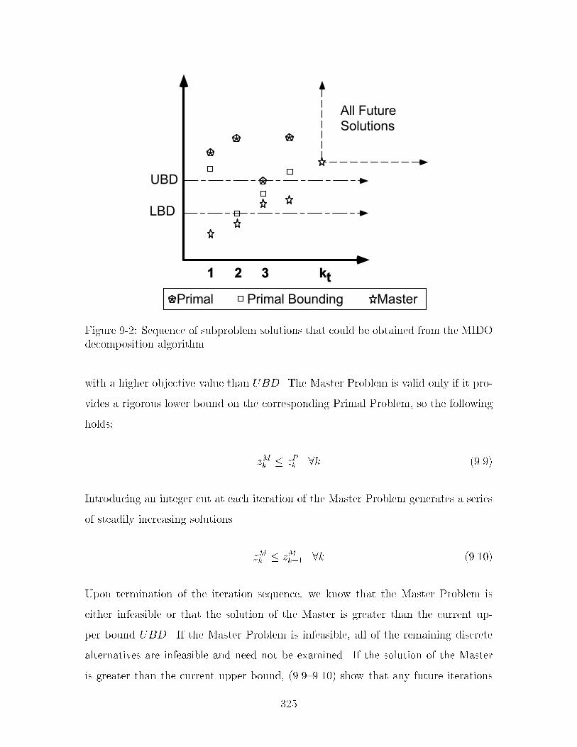
#� ��� 7���#� ����'���� ��
33 ,, .. 44
$'�
����8������� ���
�'�
Figure ��� Sequence of subproblem solutions that could be obtained from the MIDOdecomposition algorithm
with a higher objective value than UBD The Master Problem is valid only if it pro
vides a rigorous lower bound on the corresponding Primal Problem� so the following
holds�
zMk � zPk �k ����
Introducing an integer cut at each iteration of the Master Problem generates a series
of steadily increasing solutions
zMk � zMk�� �k �����
Upon termination of the iteration sequence� we know that the Master Problem is
either infeasible or that the solution of the Master is greater than the current up
per bound UBD If the Master Problem is infeasible� all of the remaining discrete
alternatives are infeasible and need not be examined If the solution of the Master
is greater than the current upper bound� �������� show that any future iterations
���
will result in solutions that are greater than the current upper bound This proves
that iteration technique is capable of avoiding total enumeration of the discrete al
ternatives� and that the discrete alternative leading to the global solution has been
investigated
Next we verify that we have obtained a bound on the distance to the global
solution We recognize that the global solution must be greater than the minimum of
the primal lower bounds LBD � mink %zPk Note that this contrasts with conventional
MINLP algorithms in which the solution of the Master problem always provides the
lower bound In conventional MINLP algorithms the global solution of the Primal
problem is guaranteed� so the lower bound can be updated after each solution of the
Master problem However� for the MIDO problem the solution of the Primal is not
guaranteed to provide the global optimum� so the lower bound can only be updated if
the solution of the Master is guaranteed to be less than the global optimum of all of
the previously examined Primal problems Since the solution of the Primal Bounding
model provides a rigorous lower bound on the solution of the Primal problem� the
lower bound can be updated after the solution of the Master problem as long as the
solution of the Master is not greater than any of the solutions of the Primal bounding
model found so far Figure �� shows that on the second iteration the lower bound
was updated after the solution of the Master problem� since zM� � %zP� However� after
the solution of the third Master problem� LBD cannot remain at the value given
by the %zP� because the possibility exists that a solution of the Primal problem with
value less than zM� exists The least upper bound is simply UBD� the in�mum of the
solutions of the primal subproblems Therefore the distance between the solution at
termination and the tightest bound we have obtained on the global solution is given
by UBD � LBD
Since zMk is forced to be nondecreasing at each step �through the introduction
of the integer cuts�� and there are a �nite number of integral realizations of yk� the
algorithm will terminate after a �nite number of iterations Depending on how tight
the screening model is� this property has the potential to avoid enumeration of the
entire discrete decision space
���

�� Casting Batch Process Development as a MIDO
This section demonstrates that the batch process development problem can be formu
lated as a mixed time invariant integer dynamic optimization problem that conforms
to ������ For illustration� the batch process development example from chapter �
is formulated according to ������
The goal of the MIDO is to select the values for the time invariant parameters and
control pro�les that minimize the production cost per unit mass of product P using
equipment that is available within the existing manufacturing facility The processing
costs are evaluated assuming cyclic steady state for the duration of the campaign�
ignoring end e�ects We employ simple dynamic models of both the distillation
column and the reactor for the purposes of illustration More complicated dynamic
models can be employed within the formulation� but they would make the expression
of all the model constraints within this text far more cumbersome In the following
model� time invariant parameters are represented by v and the controls are represented
by u The reactor temperature� the feed rate of reagent� the column re ux ratio� and
the positions of the valves governing the ow into the accumulators are treated as the
control variables in the optimization The superscripts on the controls and the time
invariant parameters indicate what the particular controls and parameters represent
Note that each task is denoted by the subscript k This di�ers slightly from the
notation employed in chapter � in which the subscript k referred to processing trains
We consider a superstructure with two distillation and reaction tasks� and let k refer
to an element taken from the ordered set K � fR�� D�� R�� D�g� and let KR and KD
refer to the order subsets of the reaction and distillation tasks Let inequality �eg�
k � k�� and arithmetic operations �eg� k � �� refer to operations performed with
respect to the ordinality of the elements of the set
We employ time invariant parameters to represent the state of the material en
tering and leaving each of the tasks These material states are represented by the
tanks surrounding each of the tasks shown in �gure �� The mass balance around
each of these tanks is enforced by constraints on the time invariant parameters Fig
���

ure �� denotes material transfers described by the model equations using solid lines
and transfers that occur at the beginning and end of the tasks using dotted or dashed
lines� these transfers are represented by point constraints in the formulation Trans
fers between these tanks are represented by point constraints in the model
)��
����
��
!��
��
!��
��
!��
��
!��
��
!��
!�� !�� !��!�� !��
�� �� �� �� �� #�����((
��
�� �� �� �� ����
((
��
�� �� �� �� ����
����
��
!��
��
!��
��
!��
��
!��
��
!��
!�� !�� !��!�� !��
�� �� �� �� ��((
��
�� �� �� �� ����
((
��
�� �� �� �� ����
Figure ��� The superstructure for the MIDO formulation of the process developmentexample from chapter �
���� Distillation Column Constraints
A simple equilibrium stage model of the batch distillation is employed �Bernot et al��
����� The model assumes no holdup on the trays� constant pressure� and does not
enforce energy balances All of the material in the column is contained in the liquid of
the reboiler The Wilson activity coe�cient model and the extended Antoine vapor
pressure model are used to determine the vaporliquid equilibrium� but have simply
���

been represented below using fVLE which de�nes the relationship between liquid and
vapor composition� pressure� and temperature We ignore utility costs in this example
in order to simplify the distillation model
The model of the distillation column contains NS equilibrium stages in the tray
section� resulting in NS "� stages The �rst stage corresponds to the reboiler� The
model of the distillation accounts for multiple columns of the same type operating
in exactly the same fashion This permits the columns to be modeled as one larger
column operating at a vapor rate that represents the sum of the individual rates
Reboiler�
dMek
dt� � V vapor
k
uRk " �xDeky
Dk �e� k � KD �����
M totalk �
Xe
Mek �k � KD �����
Mek � M totalk xeks �e� k � KD� s � � �����
V molk � fVol�xks� Tks� Pk� � k � KD� s � � �����
Equilibrium Stages�
fVLE �xks�yks� Tks� Pk� � � � k � KD� s � �� ns" � �����Xe
yeks � � � k � KD� s � �� ns" � �����
Operating Line�
xksuRk � yk�s��
�uRk " �
�� xDk � k � KD� s � �� ns" � �����
�Although this goes against the usual numbering convention� we have found that treating thereboiler as the �rst stage makes it considerably easier to provide a guess for the initial columnpro�le� since the initial pro�le from a column with fewer stages can be used as the initial guess forthe column with more stages�
���

Condenser�
xDk � yks � k � KD� s � ns" � �����
Dek � �dMek
dt� e� k � KD �����
nc��Xc��
�uScutck " uSock
� � � k � KD �����
dM cutcek
dt� Deku
Scutck � c � �� nc� �� e� k � KD �����
dMo�cek
dt� Deku
Sock � c � �� nc� �� e� k � KD �����
Note that the fraction of the distillate fed to each of the cut and o� cut accumulators
of the distillation column is speci�ed by the control variables uScutck and uSock Since all
of the distillate must be sent to the accumulators� ����� requires that these controls
sum to one The fraction of the distillate ow reaching the the splitter above each
of the accumulators that is sent to the accumulator can be de�ned as follows for the
cuts and o� cuts respectively�
Split Fraction for Cut ck �uScutck
��Pc��c���
�uScutc�k " uSoc�k
Split Fraction for O� Cut ck �
uSock
��Pcc��� u
Scutc�k �Pc��
c��� uSoc�k
The split fractions for each of the splitters �or the position of the valves directing the
ow into the accumulator� are not included as controls in the problem� but can be
calculated from uScutck and uSock easily
The operation of the column requires speci�cation of the initial conditions and any
requirements that are placed on the �nal state of the operation These constraints
follow
���

Inequality Path Constraints�
yDk Vmolk M total
k �Xi�ID
NiXn��
yCiknn %Vi �k � KD �����
� � uScutck � � �k � KD� c � �� nc� � �����
� � uSock � � �k � KD� c � �� nc� � �����
��� � uRk � �� �k � KD �����
Final Time Constraints�
Xe
M cutcek � vM
cut
ck � c � �� nc� �� k � KD �����
M cutcek � vM
cut
ck vXcut
cek � c � �� nc� �� e� k � KD �����Xe
Mo�cek � vM
o
ck � c � �� nc� �� k � KD �����
Mo�cek � vM
o
ck vXo
cek � c � �� nc� �� e� k � KD �����Xe
Mek � vMcut
ck � c � nc� k � KD �����
Mek � vMcut
ck vXcut
cek � c � nc� e� k � KD �����
Initial Time Constraints�
Mek � vMmix
k vXmix
ek � e� k � KD �����
M cutcek � � � c � �� nc� �� e� k � KD �����
Mo�cek � � � c � �� nc� �� e� k � KD �����
���� Reaction Constraints
The reaction step comprises the set of competing reactions shown below All of the
reactions are �rst order under the conditions in which the process may be operated�
���

reactions � and � are �rst order in A
A "B�� I
�� Py�
y�
W� W�
The relative rates of the reactions have been chosen so that they agree with an early
study of reaction temperature optimization �Denbigh� ����� following Arrhenius rate
expressions given by the constants in table ��
A simple dynamic model of the reactor is employed Both the temperature and
the rate at which material is charged to the reactor are treated as controls At the
completion of the reaction task the impeller is stopped� and the catalyst settles to the
bottom We assume that the reactions stop at this point Note that the model of the
standard reaction task has been augmented to include the equality path constraints
de�ning the amount of material charged from each of the feed tanks Several design
constraints restrict the operation of the reactor A molar ratio of solvent to A of
at least �� is required� the components B� W�� and W� all can act as the solvent�
and all of the solvent must be charged initially An excess of B �two times A� is also
required We assume that parallel reactors operate in phase In this model we assume
that reactors only di�er in size� so multiple reactors in parallel can be modeled as one
larger reactor� simplifying the model of the reaction task
DAE model of reaction task�
dMRin
ck�k
dt� uR
in
ck�k � c� k � KR� k� � KD �����
dMSin
ek
dt� uS
in
ek � e � ER k � KR �����
dMek
dt�
Xr�Rk
yRxnk ratekrekr " uSin
ek
���

"Xc
Xk�
uRin
ck�kvXRin
cek�k � e k � KR �����
Mek � M totalk xeks �e� k � KR �����X
e
xek � � �k � KR �����
Tk � uTk �k � KR �����
V molk � fVol�xk� Tk� Pk� � k � KR �����
V molk M total
k � Vk �k � KR �����
CekVk � Mek �e� k � KR �����
ratekr � CA�k re�EArRT � k � KR� r � �� � �����
ratekr � CI�k re�EArRT � k � KR� r � �� � �����
Inequality Path Constraints�
��� � uTk � ��� �k � KR �����
yRxnk Vk �Xi
Xn
yRiknn %V Voli �k � KR �����
�MA�k � MB�k � k � KR �����
Initial Time Constraints�
Mek �Xc
Xk�
vRinit
ck�k vXRin
cek�k " vSinitek � e� k � KR �����
MRin
ck�k � vRinit
ck�k � c� k � KR� k� � KD �����
MSin
ek � vSinitek � e� k � KR �����
Final Time Constraints�
Xe
Mek � vMRout
k � k � KR �����
Mek � vMRout
k vXRout
ek � e� k � KR �����
���

vMRin
ck�k � MRin
ck�k � c� k � KR� k� � KD �����
vSek � MSin
ek � e� k � KR �����
The design constraint on the solvent to reactant ratio can be expressed using the
following point constraint for each of the reaction tasks
��
()X
c
Xe�fA�Ig
Xk��KD
vRinit
ck�k vXRin
cek�k "Xe�fAg
vSinitek
*A �
()X
c
Xe�fB�W��W�g
Xk��KD
vRinit
ck�k vXRin
cek�k "Xe�fBg
vSinitek
*A � k � KR �����
We employ constraints expressed in terms of the integer time invariant parameters to
de�ne the process structure and a feasible allocation of equipment
Point Constraints�
Xi�ID
NiXn
yCikn � yDk �k � KD �����
Xi�IR
NiXn
zRikn � yRxnk �k � KD �����
V vapork �
Xi�ID
NiXn
yCiknn %V vapori �k � KD �����
vtcycle � tfk " yDk�t�ll " tempty " tre�ux
� �k � KD �����
vtmerged
k � tfk " yMk��vtmerged
k�� �k � KR �����
vtcycle � vt
merged
k " t�ll " tempty � k � KR �����
yDk �Xi�IR
NiXn��
zRikn � k � KR �����
zRikn � zRi�k���nyMk�� " yRikn � i � IR� k � KR �����
yMk � yDk � k � KR �����
���

� � yMk�� "NiXn
yRikn � i � IR� k � � � KR �����
Note that ����� assumes that the tasks are ordered R�� D�� R�� D�� etc In this
example the set K contains only two reaction and distillation tasks� so the subscript
k � � refers for k � KR refers to the previous reaction task and k � � refers to the
previous distillation Mass balances are enforced around each of the tanks used to
represent the material that is transferred from one task to another� and ����� ensures
that a fraction of all recycled material is purged
vMcut
ck �Xk��KR
vMRin
ckk� "Xk��KD
vCMckk� " vCPck " vCWck � c� k � KD �����
vCPck " vCWck � Xpurge
� Xk��KR�k��k
vMRin
ckk� "X
k��KD�k��kvCMckk�
�� c� k � KD �����
vXRin
cekk� � vXcut
cek � c� e� k � KD� k� � KR
�����
vMmix
k �Xe�ER
vSek "Xe
vMRout
k��
"Xc
vMo
ck "Xc
Xk��KD
vCMck�k � k � KD �����
vMmix
k vXmix
ek � vSek " vMRout
k�� vXRout
k���e
"Xc
vMo
ck vXo
cek� "Xc
Xk��KD
vCMck�kvXcut
cek� � e� k � KD �����
vSek � � � e � ER� k �����
The required product purity is enforced using the following constraint�
XproductXk�KD
Xc
Xe
vMcut
ck vXcut
cek MWe �Xk�KD
Xc
Xe�fPg
vMcut
ck vXcut
cek MWe �����
The itemized production costs can be calculated and assigned to time invariant pa
���

rameters
vRaw �Xk
Xe�ER
vSekCrawe MWe �����
vWaste �Xk�KD
Xc
Xe
vCWck vXcut
cek Cwastee MWe �����
vEquip � vtcycleXk
�Xi�IR
NiXn
yRiknnCEquipi "
Xi�ID
NiXn
yCiknn
������
The constraints de�ned by ��������� must be satis�ed The objective is listed below�
it de�nes the manufacturing cost per unit mass of �nal product
� �vRaw " vWaste " vEquipP
k�KD
Pc
Pe v
CPck vX
cut
cek MWe
�����
�� Application of the MIDO Decomposition Al�
gorithm
The Master Problem for this example is the MILP screening model for the batch
process development problem presented in chapter � The screening model determines
a feasible equipment allocation and provides initial guesses of the amounts of material
held in each of the tanks described by the time invariant parameters of the dynamic
optimization
The Primal Problem de�nes a dynamic optimization that considers the reaction
and distillation tasks and their recycles simultaneously This dynamic optimization
problem is obtained by simply �xing the integer parameters in the above formulation
at the value determined by the solution of the corresponding Master Problem The
time invariant parameters and controls are selected to minimize the production cost
per unit mass of product
We highlight several features of this problem that impact the use of dynamic opti
mization and the application of the proposed iteration technique First� the structure
of the process considered during dynamic optimization can change depending on the
���

values of the discrete variables chosen by the Master Problem We can simplify the
process structure before solving the dynamic optimization subproblem based on the
solution of the Master problem For instance� some of the processing tasks may not
exist within the current process structure In addition� we may want to consider re
ducing the number of distillation cuts permitted within the current process structure
based on the solution of the screening model Note that the superstructure de�ned
here permits for � overhead cuts� but neither solution of the screening model given in
chapter � required so many The qualitative behavior of the distillation may change
with small changes in the optimization parameters� for instance� a small change in
the feed composition to a distillation task may move the feed into a new batch dis
tillation region For this reason� we treat the active batch distillation as one of the
discrete variables characterizing the process structure� this allows us to address some
of the behavior known to lead to multimodality in the dynamic optimization during
the solution of the Master Problem
We note two applications for the Primal Bounding Model incorporated within our
algorithm First� the Primal Bounding Model provides us with a formal strategy for
employing the solutions from the global optimization of the nonconvex Primal sub
problems whenever such techniques are developed� Second� the Primal Bounding
Model provides a convenient and e�cient way in which to employ a screening model
that is posed as a convex MINLP The solution of a convex MINLP screening model
using traditional decomposition approaches such as GBD �Geo�rion� ����� or OA
�Duran and Grossmann� ����� results in an iteration strategy like the one shown in
�gure �� Rather than solving the MINLP screening model to completion on each
iteration� we can simply employ the NLP used as the Primal subproblem in the de
composition of the MINLP screening model as as the Primal Bounding model Using
this strategy� shown in �gure ��� the Master problem of the MIDO decomposition is
the same as the Relaxed Master problem used to solve the convex MINLP screening
model� the Primal Bounding Model is the convex NLP corresponding to the Primal
�It should be noted again that the global solutions to the Primal problem may not be used toconstruct valid support functions�
���

problem used to solve the MINLP screening model� and the Primal problem is the
dynamic optimization corresponding to the values of the y determined by the solution
of the Master problem At each iteration� the Master problem is augmented with the
support functions obtained from the solution of the Primal Bounding model� we can
continue to add constraints to the Master problem until the solution of the Master
problem rises above that of the Primal Bounding problem �eg� the solution of the
screening model has been determined� Using this strategy� the MINLP screening
model does not need to be solved to convergence at every iteration
������������
�� ��� ���� ���
�������
��������������������������������������
Solve for zP
k
UBD � min�UBD� z
P
k�
�
��
k � �
LBD � ��
UBD ��
���������
Solve for zM
k
Update lower bound
LBD � zM
k
zM
k� UBD
or
infeasible�
z � z�
� UBD
Figure ��� Decomposition algorithm employed for MINLP problems
��� Summary
This chapter has de�ned the class of problems termed mixed time invariant integer
dynamic optimization problems We demonstrated that simple extensions of tradi
tional MINLP algorithms are doomed to failure on this class of problems Instead�
we have developed a decomposition algorithm for this class of problems that gen
eralizes the decomposition algorithm employed for batch process development to a
���

�����
����������
Solve for zP
k
UBD � min�UBD� z
P
k�
�
������� ������������ �����
��zM
k� UBD
or
infeasible�
z � UBD
z � z�
� UBD� LBD
k � �
LBD � ��
UBD ��
���������
Solve for zM
k
Update lower bound
LBD � mink��k
�zM
k � �zPk�
�
Solve for �zP
k
���� ���7����5��&��7���
���� ���7����#� ����9�#
�%��� �� ! � :� ��
������������������������
�� ��� ���� ���
�������
Figure ��� MIDO decomposition algorithm when a convex MINLP screening modelis employed
broader class of problems The algorithm de�nes a rigorous iteration procedure that
guarantees improvement of the solution and potentially avoids explicit enumeration
of the entire discrete decision space The key to the application of this algorithm is
the ability to derive a screening model for the particular problem in which we are
interested
We have demonstrated that the batch process development can be formulated as a
MIDO problem� and derived the MIDO formulation for the batch process development
example of chapter �
�� Notation
����� Indexed Sets
C The set of distillation cuts� c � �� � � � NC
E The set of pure components in the system� e � �� � � �NC
���

ER The set of pure components regarded as raw material that may be supplied
I The set of equipment available in the manufacturing facility
ID Equipment suitable for distillation tasks ID I
IR Set of equipment suitable for reaction tasks IR I
K The set of processing tasks in the superstructure
KD The set of distillation tasks in the superstructure KD � K
KR The set of reaction tasks in the superstructure KR � K
Rk set of reactions occurring in the reaction task in processing train k In this
example� r � �� � � � �
S The set of de�ning the equilibrium stages in the column s � � � � � NS
����� Variables
Cek concentration of component e in the reaction task k
Dek molar ow of component e in the distillate of k
Mek molar holdup of component e in task k
M cutcek molar holdup of component e accumulated in cut c of task k
Mo�cek molar holdup of component e accumulated in the o� cut following cut c
of task k
M totalk total molar holdup in task k
MRin
ck�k feed to reactor k from cut c in of distillation k�
MSin
ek supply to reactor k of raw material e
ratekr rate of reaction r in task k
Vk total volume of material in task k
V molk molar volume of material in task k
V vapork e�ective vapor rate of the columns assigned to distillation task k
xek� xeks mole fraction of component e in the reactor k� mole fraction of component
e in the liquid phase of stage s in distillation k
xDek mole fraction of component e in the distillate of task k
���

ye mole fraction of component e in the vapor phase
zRkin n reactors of type i are assigned to reaction task k
����� Time Invariant Integer Optimization Parameters
yCikn n columns of type i are assigned to distillation task k
yRkin n reactors of type i begin processing reaction task k If tasks are merged�
they may also process reaction task k " �
yRxnk indicates whether reaction task k is performed
yDk indicates whether distillation k is performed
yMk indicates whether reaction task k is merged with reaction task k " �
����� Control Variables
uScutck fraction of the distillate of distillation k that is sent to the accumulator for
cut c
uRin
ck�k ow rate into reaction task k from the feed tank fed by cut c of distillation
task k�
uSin
ek ow rate into reaction task k from the supply tank containing raw material
e
uSock fraction of the distillate of distillation k that is sent to the accumulator for
o� cut c
uRk re ux ratio of distillation task
uTk temperature pro�le for reaction task k
���� Time Invariant Continuous Optimization Parameters
tfk the �nal time �eg� length of operation� of task k
vCMckk� the total molar ow from cut c of distillation k to the mixer tank that
feeds distillation k�
vCPck the total molar ow from cut c of distillation k in the product stream
���

vCWck the total molar ow from cut c of distillation k in the waste stream
vEquip cost per batch of equipment
vMcut
ck the total accumulation in cut c of distillation k
vXcut
cek the mole fraction of component e in cut c of distillation k
vMo
ck the total accumulation in o� cut c of distillation k
vMmix
k the total molar charge to the mixer tank feeding distillation k
vMRin
ck�k the total molar charge to the feed tank of reaction task k taken from cut
c of distillation task k�
vMRout
k the total molar holdup in the tank containing the e)uent of reaction task
k
vSek the total molar charge raw material e fed to reaction task k
vRaw cost per batch of raw material
vRinit
ck�k the initial charge to reaction task k taken from the feed tank fed by cut c
of distillation k�
vSinitek the initial charge to reaction task k from raw material supply tank e
vtcycle
the cycle time for process operating at cyclic steady state and employing
no intermediate storage
vtmerged
k the processing time for the potentially merged set of reaction tasks ending
with reaction task k
vRaw cost per batch of waste disposal
vXmix
ek the mole fraction of component e in mixer feeding distillation k
vXo
cek the mole fraction of component e in o� cut c of distillation k
vXRin
cek�k the mole fraction of component e in feed tank of reaction task k fed by
cut c of distillation k�
vXRout
ek the mole fraction of component e in tank containing the e)uent of reaction
task k
����� Parameters
MWe molecular weight component e
���

Ni number of equipment units i in the manufacturing facility
t�ll time required to charge one batch of material to an equipment unit
tempty time required to empty one batch of material from an equipment unit
tre�ux time required to bring a column to total re ux
%Vi processing volume of equipment unit i
%V vapori maximum vapor rate for distillation column i � ID
ekr the stoichiometric coe�cient for component e in reaction r of task k
���

���

Chapter �
Conclusions and Recommendations
This thesis has argued the importance of batch process development to the specialty
chemical and synthetic pharmaceutical industries To be e�ective� manufacturers
must rapidly develop e�cient processes The goals of rapid and e�cient development
are not necessarily mutually exclusive� and we feel that the application of state of
the art process modeling technology can reap bene�ts on these types of problems
in spite of the fact that little has been published demonstrating the bene�ts that
can be achieved through the application of detailed process models This thesis has
addressed two of the hurdles to routine application of process modeling technology
to batch process development First� a systematic and rigorous design procedure has
been derived that starts with the information provided by the laboratory synthesis
of a new product and employs models of the process at two levels of detail Second�
the numerical solution procedures required for the subproblems inside our framework
have been improved� making them more robust and e�cient
���� Screening Models for Batch Process Devel�
opment
This thesis has demonstrated that detailed discrete�continuous dynamic models can
be employed within a systematic methodology for the design of batch processes For
���

an e�ective yet practical approach� the detailed dynamic models should be used in
conjunction with simpler models capable of yielding rigorous lower bounds on the cost
of the resulting process that serve as design targets These bounding models have
been termed screening models since their solution can be used to prune or screen
discrete design alternatives that cannot lead to an optimal solution These models
address the discrete design decisions directly and replace the detailed dynamic models
with algebraic constraints that bound the dynamic performance The derivation of
these models was discussed in detail in chapter � and the models were demonstrated
on process development examples in chapters � and �
Since screening models provide rigorous bounds on the manufacturing cost� they
also permit the derivation of the �rst rigorous iteration strategy for the improvement
of the design as discussed in section �� The iteration strategy involves the solution of
the screening model followed by the dynamic optimization of the discrete�continuous
dynamic process model for the �xed values of the discrete decisions de�ned by the
solution of the screening model The solution of the screening model provides a
target for the dynamic optimization� and the solution of the dynamic optimization
�if feasible� de�nes a process design alternative in detail An integer cut is then
added to the screening model and the procedure is repeated Since the objective
value of every solution to the dynamic optimization must be greater than that of
the corresponding screening model� the iteration can be terminated once the current
screening model solution increases above the minimum of the previous solutions to
the dynamic optimization It is important to note that this algorithm generalizes to
a class of mixedinteger dynamic optimization problems� provided that appropriate
screening models can be constructed In chapter �� we also showed that this approach
provides the �rst rigorous method to address mixedinteger dynamic optimization
problems using control vector parameterization for the variational subproblem
Screening models also have the ability to address some of the synthesis decisions
involved in process design The ability to determine the best processing structure was
demonstrated by the case studies Both case studies demonstrate that the screening
models can quickly identify potentially favorable processing structures� so that de
���

tailed design e�orts can be focused on the most promising alternatives �rst In fact�
a large number of potential con�gurations may be eliminated through the use of
the screening models The screening models should capture the dominant operating
tradeo�s and design constraints in order to provide useful information� but they need
not embed all the tradeo�s in the problem in order to provide useful information
These models provide a convenient framework in which to apply limited information
about the process and automatically generate potentially bene�cial process alterna
tives that may not have been intuitively obvious to the engineer More importantly�
they provide a good starting point for detailed design and a metric against which
existing designs can be measured In fact� the information provided by the screen
ing model may be all that is required to demonstrate that further design e�orts are
unwarranted
���� Numerical Issues in the Simulation and Opti�
mization of Hybrid Discrete�Continuous Dy�
namic Systems
Stateoftheart process modeling environments place extremely high expectations on
the e�ciency and robustness of the numerical solution procedures This research
has improved both the robustness and e�ciency of the integration techniques em
ployed during the simulation and optimization of hybrid discrete�continuous dynamic
systems These improvements have been incorporated within DSL��S� a version of
DASSL �Petzold� ����a� for large sparse unstructured systems of DAEs� which was de
veloped as part of this research The code employs the MA�� linear algebra routines�
works with a combined analytic and numerical Jacobian matrix� and has incorpo
rated the automated scaling and e�cient initialization techniques described within
this thesis The code also contains an e�cient method for sensitivity analysis that
was developed by Feehery and Barton ������ The code has been implemented within
ABACUSS and is substantially more robust and e�cient than the version of DASOLV
���

�Jarvis and Pantelides� ����� employed within ABACUSS on the wide range of sim
ulations on which it has been tested
Simulations of the batch distillation of wideboiling azeotropic mixtures uncovered
some of these numerical di�culties Our investigation determined that the observed
problems were caused by an illconditioned corrector iteration matrix We found that
scaling of these models� even simply changing the units of the model variables� helped
the integration procedures substantially This motivated us to pursue automatic
scaling techniques to improve the solution procedure We demonstrated that the
desired variable scaling is dictated by the user de�ned error tolerances� and proved
that the implemented row scaling brings the two norm condition number of the scaled
iteration matrix to within a factor of �pq of the minimum possible� where q represents
the maximum number of nonzero entries in any column of the matrix The automated
scaling techniques make the model better scaled than any user implemented scaling
resulting from the selection of appropriate units of measurement In addition� the
scaling can automatically adapt to variable values changing over many orders of
magnitude during a simulation � a typical occurrence during the simulation of batch
processes The scaling also permits the code to automatically determine whether
the potential exists for the truncation error control within the integration method to
break down
Hybrid discrete�continuous dynamic simulation and dynamic optimization re
quires the integration code embedded within a simulation environment �eg� ABA
CUSS� to be started many times during a particular simulation or optimization cal
culation On these types of problems� the performance of the integration code during
the initial phase of the integration becomes more important Chapter � describes the
initialization procedure developed within this thesis Before the �rst integration step
is taken� the derivatives of the algebraic variables are determined along with the sec
ond derivatives of the di�erential variables This enables us to generate a reasonable
approximation of the step size that approaches the desired truncation error tolerance
We establish criteria that de�ne the optimal initial step length for a �rst order BDF
method� and we demonstrate that the length of a step that satis�es these criteria can
���

be determined by augmenting the system of equations solved during the corrector
iteration on the �rst integration step The implementation of this procedure does not
require any assumptions about the stability of the method at these step lengths� and
it permits the same method for the detection of implicit state events to be employed
throughout the integration Application of this method to hybrid discrete�continuous
simulation problems has demonstrated that it reduces the number of Jacobian fac
torizations required� increasing the e�ciency of the integration code Moreover� it
reduces the number of truncation error and convergence failures that are observed
The screening models derived within this research coupled with the advances in
the numerical capabilities of the solution procedures provide the engineer facing the
batch process development problem with a new and powerful approach� along with
the tools required to implement it
���� Recommendations for Future Research
Detailed hybrid discrete�continuous dynamic models of batch processes require an
accurate representation of the phenomena of interest For networks of reaction and
distillation tasks� this requires a large amount of data to represent the physical prop
erties and vapor liquid equilibrium for the system components� and to describe the
kinetics of the reactions occurring within the process Since these processes typically
involve some chemical species for which little information may be available within
existing databases� techniques to gather this data e�ciently or to estimate the key
properties are required In addition� the sensitivity of the resulting design to uncer
tainty in this data must be analyzed The sensitivity of the resulting design with
respect to these parameters can easily be performed within simulation environments
such as ABACUSS which can calculate parametric sensitivities These sensitivities
can be used to identify the parameters with the biggest impact on the process design
and to direct experimental e�orts to reduce the uncertainty in the most in uential pa
rameters The bene�ts that can be obtained through the use of process models provide
a motivation for obtaining this data Some of the chemical species� such as solvents
���

and familiar reagents may be common to many processes� so their properties may be
well understood However� the reaction kinetics and VLE data are required for the
new components The application of both computational chemistry �Bruneton et al��
����� and dynamic optimization will enable reaction kinetics to be determined from
calorimetric data in a routine fashion Similarly� advances in calorimeter technology
coupled with the increased use of in situ infrared spectroscopy have greatly reduced
the experimental e�ort required to obtain this data Computational chemistry can
be employed to screen potential reaction mechanisms� and dynamic optimization can
be employed to perform the parameter estimation In addition� it may be possible to
regress or re�ne binary VLE parameters from data obtained from laboratory batch
distillation columns using dynamic parameter estimation For modeling to be rou
tinely applied to new processes� e�cient methods are required to obtain data These
techniques should be investigated further� now that methods that require the data
are available as process design tools
The screening models that have been developed within this research address pro
cesses comprised of only reaction and distillation tasks However� many specialty
chemical and synthetic pharmaceutical processes contain other unit operations� such
as crystallization� extraction� �ltration� solvent switch� fermentation� and drying
Routine application of detailed dynamic simulation and optimization to batch pro
cesses requires development of model libraries for these common batch processing
operations In addition� to increase the applicability of the screening models� suitable
models that bound the dynamics of these operations should be developed Further
more� to deal with the detailed modeling of operations such as crystallization� im
provements to hybrid modeling environments are required to handle the distribution
of the particle sizes More importantly� the separation targets only consider homoge
neous mixtures� yet many specialty chemical processes contain heterogeneous �LLE or
VLLE� mixtures To extend the modeling approach to such systems� the batch distil
lation targeting theory must be extended to heterogeneous systems� and capabilities
for discrete�continuous dynamic models to detect the appearance and disappearance
of liquid phases and to change the model appropriately during the dynamic simulation
���

are required Both are active research topics
A systematic or automated methodology to derive targets for the reaction tasks
is also desired Currently the targets are developed on a case by case basis by iden
tifying key operating tradeo�s and capturing these within the screening models �see
chapters � and �� Reactor targeting techniques have been developed to de�ne the
attainable region that can be achieved by di�erent continuous reactor con�gurations
�PFRs and CSTRs�� but this research relies on geometric arguments and has only
been able to consider two and three dimensional �component� systems �Hildebrandt
and Glasser� ����� Hildebrandt et al�� ����� Glasser et al�� ����� Hildebrandt and
Biegler� ����� Other research has examined de�ning the reactor targets via the so
lution of a dynamic optimization problem �Hatipoglu and Rippin� ����� Balakrishna
and Biegler� ����a� Balakrishna and Biegler� ����b� Balakrishna and Biegler� �����
Sund and Lien� ����� However� the inherently nonconvex nature of the dynamic
optimization presents a major problem if the desired rigorous bounding properties
are to be guaranteed Extensions of the geometric approaches to handle higher di
mensional systems and to account for optimal temperature pro�les and feed addition
rates for fed batch reactors may permit a systematic methodology to develop targets
for the reactors A key to this development is the extension of current geometric tech
niques to capture the time�temperature tradeo�s in conjunction with the conversions
between competing reactions
The fact that screening models enable a rigorous iteration procedure for mixed
integer dynamic optimization �MIDO� problems opens up the possibility of deriving
screening models to address other classes of MIDO problems such as the synthesis of
operating procedures �Rivas and Rudd� ����� The goal in the synthesis of operating
procedures is to de�ne a cost e�ective� safe� and operationally feasible way to move
the process from one operating state to another This requires sequences of valve
and pump operations to transfer material between the equipment items allocated to
processing tasks through complex piping networks �Foulkes et al�� ������ and the ma
nipulation of control pro�les for the processing units Synthesizing such sequences
can be a di�cult task where the associated risks are high� products or valuable inter
���

mediates may be contaminated by incorrect operations� or extremely dangerous situ
ations might be created from accidentally mixing chemicals that should be kept apart
�Lakshmanan and Stephanopoulos� ����� In batch plants� it requires procedures
to ensure the safety of operations such as the startup of batch distillation columns
and the charging of reactants given the control system implemented in the plant
Validation alone requires detailed hybrid simulation of the entire process �Crooks
and Macchietto� ����� Simulation provides the means to evaluate the feasibility of
proposed procedures� but the synthesis of these procedures de�nes a dynamic opti
mization problem in terms of both discrete and continuous decisions The continuous
decisions relate to the set points for controllers� the ows of steam and cooling water
�or the settings for the control valves� to di�erent equipment units� and the de�nition
of control pro�les for all of the units within the facility Discrete decisions relate to
valves that are either open or closed� pumps and other equipment that is either on
or o�� control systems that are either in manual or automatic mode� and whether
speci�c units are used or idle These problems remain very di�cult� but the recent
results can yield parametric sensitivities for hybrid discrete�continuous dynamic sys
tems �Barton� ����� Coupling these sensitivities with screening models may enable
these problems to be investigated within a MIDO framework
Batch process development also requires a large quantity of data to describe the
equipment within the processing facility� to describe the processing operations� to
de�ne the operating policies� and to de�ne the schedule for the manufacturing facil
ities equipment The ability to manage this data is a di�cult task� and a software
environment both to manage the data and access the appropriate numerical tools is
required The environment must have facilities to specify the process models� access
the numerical tools� and analyze the results
A central feature of such an environment is the representation of the batch process
and the batch plant The tools incorporated within the environment will rely upon
seamless communication with the information stored in these models The plant can
be represented by a graph where the nodes represent physical items of equipment
�including reactors� distillation columns� valves� pumps� sections of pipe� etc� The
���

arcs of the graph represent the connections between these items The graph should
contain the information typically found in a process and instrumentation diagram
The process can also be represented by a graph� a hierarchical state task network
�STN� can be used to describe the process at multiple levels of detail �Allgor et al��
����� Processing tasks will require models� possibly several models at di�erent levels
of detail� to describe the physical and chemical transformations that can occur within
the task
Since both the plant and the process will be described by graphs� it is natural to
build these models using graphical methods Furthermore� high level communication
between the engineer and the software is essential for the development environment
to speed the engineer�s design procedure Earlier in this research we investigated a
framework with which to represent the processing facility We developed the notion
of an equipment class Each item of equipment within the processing facility is
described as an instance of a particular equipment class The equipment classes
can be constructed in a hierarchical fashion Each equipment class is speci�es the
class that it inherits from� new attributes for the class� and the instances of contained
classes and their interconnections The plant was described as an instance of an
equipment class We developed a graphical environment within which the equipment
classes could be constructed� but this area of the research was not pursued further
For many specialty chemical and synthetic pharmaceutical processes the manage
ment of the data representing the process is a major concern Creating an environment
that provides a framework to capture and store the knowledge about the process and
the current process design is essential The model would then provide a uni�ed frame
work in which to represent the process over the entire lifetime of the process This
environment can then generate descriptions of the process recipe in the form required
for the individuals working on the process� and maintain versions of the process that
are constructed as the design procedure continues Process design tools for batch
processes have recently been developed such as the BatchDesignKit �Linninger et
al�� ����a� Linninger et al�� ����b� and BATCH PLUSTM �Aspen Technology� Inc�
������ but they need to evolve to a state that permits the seamless integration of
���

process models at several levels of detail and permits access to both sophisticated
scheduling algorithms and detailed dynamic simulation and optimization
���

Appendix A
Matrix and Vector Norm Proofs
This chapter contains proves some vector and norm properties that are exploited
within the thesis These theorems are not new� but the proofs have been provided to
aid the reader in understanding the proofs contained in the body of the thesis
Theorem A � For D � Dn� x � X� and k�k� an absolute �Bauer et al� � �
vector norm� then the following holds�
minjjdjjj kxk � kDxk � max
jjdjjj kxk �A��
Proof� De�ne the vectors z � minj jdjjjx and .z � maxj jdjjjx For every component
i of Dx� the following hold
minjjdjjjjxij � �Dx�i � max
jjdjjjjxij �A��
jzij � �Dx�i � j.zij �A��
Since the norm is absolute� �A�� shows that kxk � kDxk � k.zk
Note that all of the H+older pnorms are absolute� so this holds for the norms in which
we are interested
Theorem A � maxj���AH�j
���� kAk�
���

Proof� Let ej represent the jth column of the identity matrix We also know that
kAk� ���AH
����Bauer et al�� �����
maxj
���AH�j���
� maxj
��AHej���
�A��
� maxx�fej � j��������mg
��AHx���
kxk��A��
� supx�X
��AHx���
kxk��A��
���AH
���
�A��
Theorem A � kAk� �pm���AH�j
���
Proof� We use the relationship between the two norm and the Froebenius norm
�Golub and Van Loan� �����
kAk� � kAkF �
sXi
Xj
aij �A��
�
qk�AH��k�� " k�AH��k�� " � � �" k�AH�mk�� �A��
�rmmax
jk�AH�jk�� �A���
�pmmax
j
���AH�j���
�A���
The following theorem is used to avoid the square root operation when calculat
ing the two norm of the rows of the iteration matrix during the automated scaling
algorithm
Theorem A � De�ne Z as the set of integers� Let p� q � Z and x� r� � � R where
� � � � � and q � �� We de�ne p � bxc and �� so x � bxc " � � p " �� We de�ne
r � pq � bpqc � �q � ��q� The following holds for all q � ��
x
q
!�
bxcq
!�A���
���

Proof� Expand the right hand side and use the relationship that for a � Z and y � R�ba " yc � bac" byc
x
q
!�
p" �
q
!�A���
�
p
q
!"r " �
q
!�A���
�
p
q
!"q � � " �
q
!�A���
�
p
q
!"
q � � " �
q
!�A���
�
p
q
!�
bxcq
!�A���
However� by de�nition bxqc � bbxc qc� so equality must hold
A�� Comments on condition numbers� inf� sup�
and rectangular matrices
The ratio sup� �A� inf� �A� can be de�ned for any matrix A When A is square
and invertible� we can de�ne A�� Let v � Ax and we have inf kAxk kxk �
inf kvk kA��vk This can be rewritten as sup kA��vk kvk � kA��k For the two
norm this quantity takes on the familiar form kAk� kA��k�� and we can see that the
condition number is the ratio of the largest to smallest singular values We de�ne
kA��k� �� for singular A� which makes sense when we examine the the SVD of A
The same de�nition is employed for other norms� knowing that consistent norms are
related �Golub and Van Loan� ����� The condition number de�ned on the two norm
has useful properties since it relates to the diagonal form of the matrix
���

���

Appendix B
Solution of an augmented system
of linear equations
Consider the following linear system of equations�
��A c
rT e
���zh
� �
��bf
� �B��
where A � Rn�n � c� r� z� b � Rn � and f� h� e � R� Assume that A is nonsingular and
that it has been factored� so that linear systems of the form Az � b can be solved
e�ciently This implies that �B�� can be solved without factoring the entire matrix
The �rst n rows of �B�� can be expressed as follows�
z � A���b� hc� �B��
Substituting the expression for x from �B�� into the last row of �B�� yields the
following�
h�e� rTA��c� " rTA��b � f �B��
���
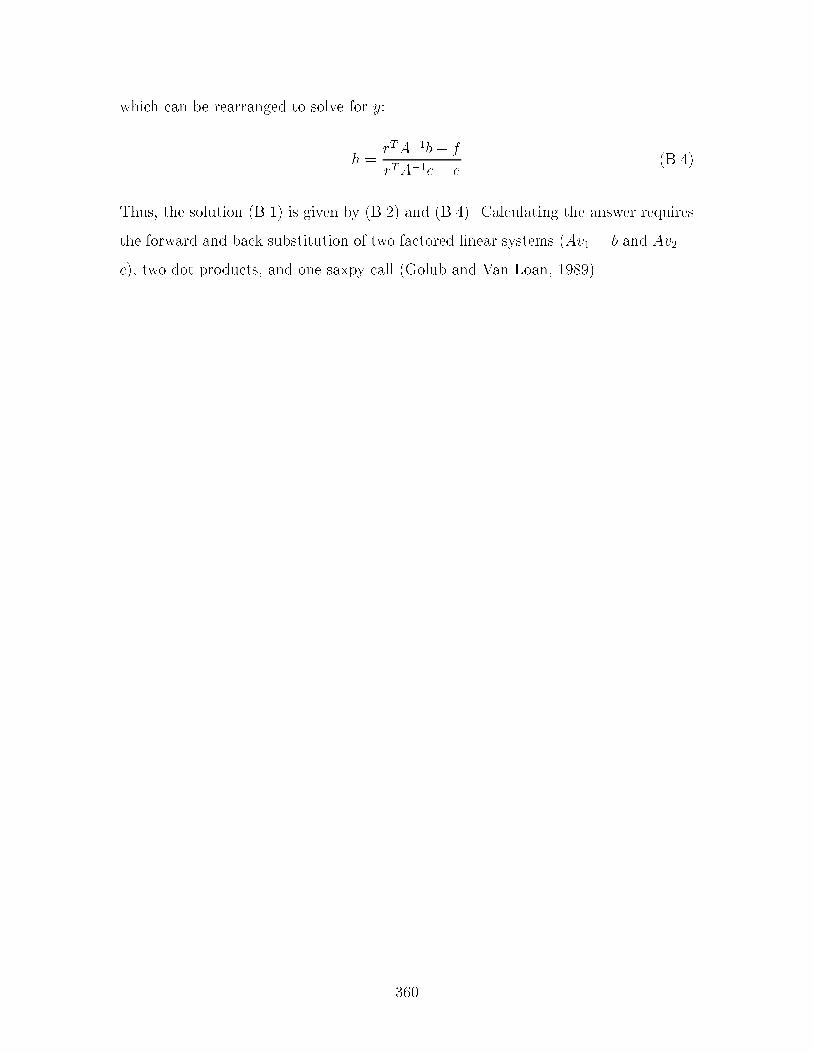
which can be rearranged to solve for y�
h �rTA��b� f
rTA��c� e�B��
Thus� the solution �B�� is given by �B�� and �B�� Calculating the answer requires
the forward and back substitution of two factored linear systems �Av� � b and Av� �
c�� two dot products� and one saxpy call �Golub and Van Loan� �����
���

Appendix C
Time derivatives of the algebraic
sensitivity variables
The linear system that de�nes the time derivatives of the algebraic sensitivity variables
di�ers from ���� in only the right hand side vector
The sensitivity equations corresponding to the parameter p are de�ned by taking
the di�erential of the DAE model with respect to p as follows �since �u�p � ���
�f
� $x
� $x
�p"�f
�x
�x
�p"�f
�y
�y
�p"�f
�p� � �C��
The values �x�p and �y�p are referred to as the di�erential and algebraic sensitivity
variables for the parameter p Di�erentiating �C�� with respect to time yields the
following�
��f
� $x�t
� $x
�p"�f
� $x
�+x
�p"
��f
�x�t
�x
�p"�f
�x
� $x
�p"
��f
�y�t
�y
�p"�f
�y
� $y
�p"
��f
�p�t�C��
which can be evaluated at to to de�ne the derivatives of the algebraic sensitivity
variables as shown below�
���

h�f� �x
�f�y
it�to
����x�p
� �y�p
�t�to
� ����f
� $x�t"�f
�x
�t�to
� $x
�p
����t�to
� ��f
�x�t
����t�to
�x
�p
����t�to
� ��f
�y�t
����t�to
�y
�p
����t�to
� ��f
�p�t
����t�to
�C��
The right hand side of �C�� needs to be provided to the integration code in order to
solve for the derivatives of the algebraic sensitivity variables Although this requires
the second order derivatives of the DAE equations� only equations in which time
appears explicitly can contribute to the right hand side �ie� those containing controls
or time� Since time often does not appear explicitly� or may only appear in a few
equations� the right hand side vector may be easily calculated in many cases If time
appears explicitly in many equations� the e�ort required to evaluate the right hand
side may not be worth the bene�ts that are obtained by calculating the derivatives
of the algebraic sensitivity variables
If a routine is provided to calculate the right hand side of �C��� DSL��S will
determine the derivatives of the algebraic sensitivities
���

Appendix D
Review of Batch Plant Design
Literature
What is commonly referred to as the �Batch Plant Design Problem� is the problem of
minimizing the investment cost required to purchase a set of equipment items in order
to meet a �xed set of production requirements This deterministic design problem
was �rst addressed by Ketner ������ and later by Loonkar and Robinson ������
����� Their original formulations of the batch plant design problem were fairly
restrictive with respect to the types of operating alternatives that were considered�
they considered only simple processing scenarios Subsequent research has focused
on considering more sophisticated operating strategies during the plant design The
progress on this problem has recently been reviewed by Rippin ������ and Reklaitis
������ The growth in the list of publications in this area since Rippin�s previous
review �����a� demonstrates that a signi�cant amount of research has been conducted
over the last ten years However� progress in these areas has been incremental� and
to this date a rigorous formulation of the problem that accounts for all possible
alternatives has not been found
The objective in the plant design problem is typically stated as the minimization
of investment cost which consists of the costs to install the batch� semicontinuous�
and continuous equipment in the processing facility� detailed aspects of the design
such as the instrumentation� and the connecting pipes and valves are typically ig
���

nored Recently� however� systematic approaches to determine the optimal layout
of the processing equipment has been considered �Jayakumar and Reklaitis� �����
Jayakumar and Reklaitis� ����� This objective is minimized subject to production
and operating constraints The production constraints usually specify the amount of
each product required within a given time horizon� and the operating constraints are
used to insure the feasible operation of the proposed design The engineer is faced
with the task of determining a way to minimize the objective within the operating and
production constraints imposed on the system These engineering decisions have been
decomposed by Reklaitis ������ into the following hierarchy of design subproblems�
� Determine the recipe task network
� Select the best operating strategy �single product� multiproduct� or multipur
pose�
� Create the equipment con�guration �storage locations� parallel units� and the
assignment of units to processing stages�
� Size equipment and determine the cost of the design
When analyzing the progress that has been achieved on the batch plant design prob
lem� it may be useful to examine the improvements made to each of the subproblems
de�ned above This view of the design problem is useful when analyzing the way
in which particular instances of the design problem are solved In fact� many of the
heuristic solution methodologies applied to this problem utilize a similar decomposi
tion of the decision tasks
Rippin �����a� has proposed a di�erent way to classify batch processing problems
that focuses on what facets of the batch process design is to be addressed The
components of the problem statement dictate what decisions and�or assumptions
the engineer must make The components of the problem considered by Rippin are
organized into the following classes�
product requirements Requirements for products are speci�ed in quantity and
time Time horizons for products may be given� or the production may have
���

to meet a set of delivery dates In some cases the demand may be uncertain
requiring added exibility in the design
process tasks These are identi�able operations carried out on the system compo
nents The mode of execution �ie� batch� must be given along with the se
quence of tasks to be carried out The performance of each task �ie� operating
conditions� must also be determined Often times these items are given as a
product �recipe� and assumed �xed during the design procedure
system structure The types� sizes� and number of equipment items must be de
termined Tasks must be assigned to equipment items or groups Constraints
on the sequencing of tasks must be enforced Product campaigns or a detailed
production plan is required The role of intermediate storage must also be
considered
design objective The cost objective must be formulated
solution methods Exact and heuristic methods are considered The tradeo�s be
tween e�ciency and accuracy must be balanced
Rippin partitions each of these categories into its essential elements� and examines the
way in which each of the elements is ful�lled The variation in the way these elements
are ful�lled describes the di�erent design problems that have been addressed Rip
pin�s method of classi�cation is useful for analyzing which design problems have been
studied� it demonstrates that improvements to the original �batch design� problem
have focused primarily on the following areas�
� Considering multiple products
� Including the cost of semicontinuous units
� Using parallel units both inphase and outofphase
� Utilizing multipurpose operating procedures
� Varying the task to stage assignment
� Accounting for discrete equipment sizes
���

� Incorporating intermediate storage and accounting for its cost
� Planning for uncertainty in the design
� Varying the solution methods used
The impact each of these items has had on the formulation and solution of the �batch
plant design problem� will be covered in the rest of this section
D�� Multiple Products
The �rst attempt at systematically minimizing the capital investment for a batch
process was undertaken by Loonkar and Robinson ������ They considered the capital
cost of the batch and semicontinuous equipment for a single product plant Given a
�recipe� for the product consisting of a sequence of operations and processing times�
the challenge was to �nd the equipment sizes which minimize the cost of the plant
The optimal cost was determined using calculus to derive the �rst order necessary
conditions for optimality� the resulting set of equations was then solved to obtain an
optimum of the convex programming problem The authors extended this idea to
multiproduct plants producing products in single product campaigns �Robinson and
Loonkar� ����� All the products manufactured must follow the same sequence of
processing steps� but some of the products may not require certain processing stages
A multivariable direct search was used to solve for the optimum value of the objective
function In both of these formulations it was assumed that the equipment is available
in a continuous range of sizes
With few exceptions� the batch process design problems addressed after ���� have
dealt exclusively with multiproduct and multipurpose plants One notable exception
is the work of Yeh and Reklaitis ������ In their work the authors focused on issues
relating to the synthesis of the process structure� so they chose a single product plant
to eliminate many of the production planning aspects which complicate the problem
���

D�� Semicontinuous units
The initial work on the batch process design problem considered the cost of semicon
tinuous equipment in the objective function �Ketner� ����� Loonkar and Robinson�
����� Robinson and Loonkar� ����� Most of the recent work addressing this problem
has ignored the costing and sizing of the semicontinuous units based on the following
three assumptions�
� The cost of semicontinuous equipment is negligible compared to the cost of the
batch units �Suhami and Mah� �����
� The cost of the semicontinuous equipment is relatively constant over the range
of plant con�gurations being considered in the design problem� therefore� it can
be removed from the objective function �Vaselenak et al�� �����
� The semicontinuous units will usually be selected based on criteria other than
cost such as safety or prior experience �Sparrow et al�� �����
The cost of batch equipment is typically a function of equipment type and volume and
the cost of semicontinuous equipment is expressed as a function of processing rate
In the work of Loonkar and Robinson ������ ����� the inclusion of semicontinuous
units was necessary to facilitate their solution procedure Since the operation times
of the semicontinuous equipment items are a function of the processing rate� they
treated the processing rates of the semicontinuous units as the decision variables of
the problem
In contrast to this� Sparrow et al� ������ chose to ignore the costing and sizing of
the semicontinuous units They state that these units will be chosen on the basis of
safety or past experience� and their selection will not in general be dictated by cost
Even though the size of the semicontinuous units will determine the time required
to transfer material to and from the vessels� most recent formulations have assumed
that the emptying and �lling times are �xed and are not functions of the volume of
material processed The processing rate of the equipment can be selected to meet
the assumed �lling and emptying times without signi�cant changes to the cost of the
semicontinuous units that need to be purchased
���

One exception to the trend of ignoring the semicontinuous units is the work of
Knopf et al� ������ They consider the design of a cottage cheese process in which the
cost of operating the semicontinuous units �separatorhomogenizerpasteurizer units�
is substantial The operating and investment costs for these units are considered in
the objective function� and these costs drive the design decisions
More recently� Yeh and Reklaitis ������ have incorporated the cost and sizing of
the semicontinuous units in order to calculate the cycle times of stages of the process
ing Their research focused on the synthesis of a superstructure for the batch process�
where the selection of the task to stage assignments may have a signi�cant a�ect on
the number of semicontinuous units� such as pumps� which are required However�
they drew no conclusions about the need to accurately express the costing and sizing
of the semicontinuous units� although it is clear that the appropriate merging of tasks
may eliminate some of the semicontinuous units from the process structure �Patel
et al�� ����� Similarly� Modi and Karimi ������ include semicontinuous units when
considering �nite intermediate storage They account for the costing and sizing of
the semicontinuous units� but the heuristic procedure which they use to optimize the
design is based partly on the assumption that the cost of a semicontinuous unit is far
less than that of a batch unit
While the assumptions regarding the relative costs of the semicontinuous units
may be valid under certain circumstances� the treatment of the issue points out that
the plant design problem will need to be evaluated for the speci�c case at hand� and
solution procedures should only be applied where they are applicable The important
costs of any design problem will most likely need to be considered on a case to case
basis
D�� Parallel Units
The processing tasks for a particular product are executed in one or more of the
equipment items existing in the plant Typically� a task or group of tasks is assigned
to a processing stage� and then one or more equipment items is assigned to this
���
processing stage for a particular product
Every processing stage must be assigned an item or group of items in which the
processing tasks will be carried out If one equipment item is assigned to a particular
stage� the only design decisions required are the selection of the size and type of unit
assigned However� if more than one unit is assigned in parallel� several decisions
must be made
� How many items in parallel are to be used
� Are the units to be operated inphase or outofphase
� Should the units in parallel be of the same size
Considering parallel units in the process structure increases the combinatorial com
plexity of the design problem and may require the use of tailored optimization proce
dures Since the complexity typically governs the performance of the solution proce
dures� problem simpli�cations that reduce the complexity� or tailored solution algo
rithms are often required If the type of parallel units considered is limited in some
way� then the complexity is reduced and solution methods that take advantage of this
simpli�cation may be employed For this reason� the type of parallel units considered
has been limited in much of the research that has been conducted so far
The �rst paper to address the use of parallel units was written by Sparrow et al�
������ The authors extended the formulation of Robinson and Loonkar ������ by
considering the addition of identical parallel units at each stage operating out of phase
Units used in this fashion serve to reduce the cycle time of a particular processing
stage and have been studied by many other authors �Grossmann and Sargent� �����
Knopf et al�� ����� Suhami and Mah� ����� Yeh and Reklaitis� ����� Vaselenak et al��
����� Faqir and Karimi� �����
The use of parallel units operating in phase has been considered by relatively
few studies Flatz ������ ����� mentions the use of in phase parallel units� but his
evolutionary design procedure does not systematically attempt to account for their
use Yeh ������ demonstrates that there is no incentive to use in phase parallel units
or units of di�erent size operating in parallel for the design of single product plants
���

Papegeorgaki and Reklaitis �����a� ����b� are the �rst to include the use of in
phase parallel units in a systematic fashion� their formulation of the multipurpose
design problem accounts for the use of in phase parallel units which may di�er in
size They formulate the problem as an MINLP with integer variables representing
the use of a particular unit for a given task In phase parallel units are included
by forming product groups which can contain units of di�erent sizes These prod
uct groups are then assigned to particular tasks with groups assigned to the same
task operating out of phase However� incorporating this exibility through the use
of integer variables rapidly increases the combinatorial complexity of the problem�
rendering current MINLP solution procedures ine�ective in the problem solution In
addition to the added complexity� the structure of the constraints yields a problem
with a considerable amount of degeneracy which places an additional burden on the
solution technique To avoid some of the degeneracy� additional constraints are added
to the formulation Papageorgaki details an approximate solution procedure designed
speci�cally for this problem �Papageorgaki and Reklaitis� ����b�
D�� Multipurpose Plants
The extension of the design problem to multipurpose plants requires fairly detailed
aspects of the production planning problem be solved at the design stage� simul
taneously with the sizing and structural aspects of the design The de�nition of a
multipurpose plant has not been agreed upon by all researchers in the �eld A mul
tipurpose plant will provide the most exible plant designs where di�erent batches
of the same product may follow di�erent routes through the plant The following
de�nitions will be used in an attempt to avoid confusion with the use of these terms�
Multiproduct Plant A plant producing more than one product in the form of single
product campaigns Every batch of a given product follows the same route
through the plant
Multipurpose Plant with Single Production Routes The plant consists of many
processing stages each having multiple identical batch units each operating in
���

parallel� out of phase Every product passes through a �xed subset of these
stages� thus� each product follows only one production route and every batch of
a given product has the same size �Faqir and Karimi� �����
Multipurpose Plant with Multiple Production Routes In this case each prod
uct may have follow multiple routes through the process A given product may
have multiple batch sizes corresponding to di�erent processing routes �Faqir
and Karimi� �����
Multi�plant Plant A plant where the equipment items are permanently partitioned
into parallel processing trains
Multipurpose Plant The most general form of processing A given product need
not follow the same processing path from one batch to the next The same
equipment may be reused for di�erent tasks of the same product Equipment
items may be shared between products during the same production campaign
The initial work attempting to address multipurpose plants was performed by
Suhami and Mah ������ They proposed a design formulation for a multipurpose
plant with single production routes� they only considered multiple products within a
campaign if they could be processed via parallel production routes They developed
a heuristic procedure to generate sets of �compatible� products� those which do not
share any equipment items� to be processed in each campaign Groups of these com
patible product sets were formed such that each group covered all of the products
to be produced For each group of product sets� the appropriate horizon constraints
were developed according to some heuristic rules The resulting MINLP was then
solved for each product group The lowest cost solution was considered the optimum
Several years later� Imai and Nishida ������ presented a way to systematically deter
mine the best group of product sets They determined the best group of product sets
by solving a set partitioning problem They generated the horizon time constraints
from this set� but did not detail the method used to derive the constraints
Vaselenak et al� ������ extended the previous work by developing a multiperiod
formulation which uses a superstructure to embed all of the possible product con�gu
���

rations They employ a systematic procedure to derive the maximal set of compatible
products which is used to generate the horizon constraints based on the available pro
duction time for each equipment unit These constraints are then �merged� to form
an equivalent set of constraints that treats the portion of the horizon time allotted
to each product as the independent variables The resulting superstructure creates a
single MINLP which can be solved for the optimum The authors realize that only
in some cases� the �fully merged� case� will the derived horizon constraints result in
a relaxed NLP which is convex Thus� in many of the cases� they cannot guarantee
optimality of their solution
Faqir and Karimi ������ attack the work of Vaselenak These authors formulate a
programming problem to address the same problem as that of Vaselenak Their for
mulation results in a single MINLP� and the formulation does not depend on whether
the horizon constraints can be �fully merged� �Vaselenak et al�� ����� This proce
dure involves fewer variables and constraints than the method of Vaselenak� and the
equivalence of their resulting formulation and the original one based on the horizon
times of each equipment item can be formally proven However� the relaxed NLP
may not be convex� so this method also cannot guarantee a globally optimal solution
Thus� it can be seen that even for the relatively simple case of single production route
multipurpose plants� a globally optimal solution cannot be guaranteed
Later� Faqir and Karimi ������ extend this idea to plants with multiple production
routes� they consider all of the possible routes that a each product can follow through
the plant and group these into sets of compatible production routes A similar method
for deriving the horizon constraints and solving the resulting problem is employed
The resulting problem is more complex� and once again a globally optimal solution
cannot be guaranteed Kiraly et al� ������ address a very similar problem� but they
employ a twostep decomposition strategy to arrive at the optimal investment cost
The aforementioned formulations can only handle situations where the equipment
items can be allocated to parallel processing trains� each representing a particular
production route� in every campaign considered
���

D� Varying the Task to Stage Assignment
One aspect of batch processes which makes them particularly exible is the distinction
between the plant and the process A manufacturing process is free utilize the plant in
the most appropriate way for every product it produces While the processing tasks
are de�ned for each product� the way in which to implement them on the plant is
not A processing stage may be assigned single or multiple processing tasks Yeh and
Reklaitis ������ showed that selecting the optimal task to stage assignment enables
more e�cient use of the processing equipment� but adds complexity to the design
decisions Even though the optimal assignment may greatly improve the e�ciency of
a design� the task to stage assignment problem has been overlooked in most of the
batch plant design literature
Papageorgaki and Reklaitis �����a� are the �rst to consider the task to stage
assignment within the plant design of multipurpose plants In fact� they are the �rst
to formulate the design for a plant operating in true multipurpose fashion They
account for multiple production routes� the use of an equipment item for di�erent
tasks within the same production campaign� and for the use of in phase and out
of phase parallel items of equipment at each processing stage Their formulation
seems superior to any others proposed thus far� but the number of integer variables is
excessive They have found that standard MINLP solution techniques fail miserably
when applied to this problem� usually yielding solutions which are inferior to those
determined by much simpler formulations of the design problem Since the problem is
so di�cult to solve� the added exibility within this formulation cannot be exploited
The authors address this problem by proposing a method to decompose and solve
the MINLP to near optimality in a companion paper �Papageorgaki and Reklaitis�
����b�
���

D� Discrete Equipment Sizes
Much of the equipment purchased for a new batch plant will be chosen from a set
of standard equipment sizes However� in many of the programming formulations of
the batch plant design problem� standard equipment sizes have been overlooked in
order to facilitate the solution of the problem In fact� the size of the equipment to be
purchased in a batch plant has been considered a continuous variable in many of the
formulations of the batch design problem �Robinson and Loonkar� ����� Grossmann
and Sargent� ����� Suhami and Mah� ����� Birewar and Grossmann� ����� These
authors usually state that the equipment can be rounded up to the next standard
size to produce a realistic feasible design
On the other hand� some authors have demonstrated that simply rounding the
optimal equipment sizes found in a continuous solution up to the next standard size
will not necessarily produce an optimal design In order to account for this� these
authors have explicitly considered the discrete equipment sizes in their problem for
mulations �Sparrow et al�� ����� Flatz� ����� Faqir and Karimi� ����� Incorporating
the standard equipment sizes explicitly in the problem formulation adds combinatorial
complexity to the problem which usually increases the solution time
Recently� however� the initial justi�cation for incorporating standard equipment
sizes� to make the problem more realistic� seems to have given way Grossmann et
al� ������ have shown that many design problems which involve nonlinear separable
objective functions and bilinear constraints can be reformulated The formulations of
Voudouris and Grossmann �����a� ����b� take advantage of the discrete equipment
sizes to transform the NLP �Grossmann and Sargent� ����� or MINLP �Birewar and
Grossmann� ����� formulations into a mixed integer linear programming problems
�MILP� The MILP formulations have the advantage that they can be solved to
global optimality Also� the methods used to solve these problems are more robust
than those that attempt to cope with nonconvex NLPs
In many cases the MILP problem contains no more variables than the original
problem and can be e�ciently solved by taking advantage of the special structure
���

of the design problem In other cases� such as the formulation of Faqir and Karimi
������� converting the bilinear constraints into an equivalent set of linear ones re
quires the addition of many variables In these situations� the MILP which must be
solved is considerably larger than the original MINLP� and the bene�ts of the trans
formation are not quite as clear� although global optimality of the solution can still
be guaranteed
D�� Intermediate Storage
Intermediate storage is often used in batch processes to reduce the amount of idle
time processing stages by partitioning the plant into two or more processing trains�
each with its own batch size and cycle time The processing rate of each of the trains
must be equal to insure that the size of the intermediate storage remains �nite In
order to employ intermediate storage� two basic decisions need to be made�
� Determine the location of the intermediate storage
� Determine the size of intermediate storage required at each location
In many design problems the cost of intermediate storage is ignored� and the
storage is located according to several scenarios � unlimited intermediate storage
�UIS�� no intermediate storage �NIS�� or zero wait �ZW� In such cases the size and
cost of the required storage is not of primary concern and is not considered when
choosing between design alternatives
Takamatsu et al� ������ �rst addressed the problem of determining the amount of
storage required to decouple two processing trains They demonstrated that the min
imum required storage is a function of the batch sizes and cycle times of the upstream
and downstream units� the initial holdup in the tank� the �lling and emptying rates of
the storage vessel� and the lag time between the two batch units They showed that
the optimal storage cost is a discontinuous function of the batch sizes and calculated
the optimal storage size when the �lling and emptying rates of the storage tank are
equivalent The minimum storage size was given as a function of the greatest com
���

mon measure of the batch sizes and the lag time between units Karimi and Reklaitis
������ considered a similar case where the �lling and emptying rates of the tank are
not equal They determined the minimum storage requirement by �rst deriving an
analytical solution to the di�erential equation describing the tank holdup via Fourier
series analysis� ignoring any changes in volume upon mixing With this solution� they
determined the minimum and maximum values of the holdup Karimi and Reklaitis
������ built upon this work by determining the minimum volume requirement for a
processing network in which the number of parallel units both upstream and down
stream of the storage may vary They calculated the lag time policy which minimizes
the storage requirement More importantly� they generated a simple upper bound� in
dependent of the lag time policy employed� for quickly estimating the storage volume
requirements
The optimal sizing of intermediate storage within a multiproduct plant has been
addressed by Modi and Karimi ������ The authors developed a method which con
siders the cost and sizing of intermediate storage during the design stage of a multi
product plant The heuristic procedure used is based on deriving an initial design and
then improving on it by adjusting the processing rates of the semicontinuous units�
the number of batch units at each stage� and by varying the allocation of the total
production time allotted to each product However� this method does not explicitly
address the location of the storage within the process The method must be run
repeatedly� with storage at di�erent locations� in order to determine the best location
for the storage
Yeh and Reklaitis ������ addressed the issue of storage location for a single prod
uct plant Heuristic rules to identify the best locations for additional intermediate
storage are de�ned� intermediate storage is located in order to maximize the equip
ment savings for the processing train not containing the time limiting stage The
sizing procedures for the storage are not detailed� but the bound presented by Karimi
and Reklaitis ������ can be employed
An interesting use of intermediate storage was considered by Shah and Pantelides
������ They note that multiproduct plants operating in campaign mode often con
���

tain products with stable intermediates If longterm storage is available� as it is for
the products� then these intermediates may be produced as the product of a given
campaign When these intermediates are used in the production of several products�
the value of producing them in their own campaign is obvious They demonstrate
that even in the cases where the intermediate is only used by one product� producing
it in a campaign is often bene�cial because it may allow other intermediates to be pro
duced at the same time However� the MINLP programming formulation presented
only considers such processing structures for single product plants
Another bene�t of intermediate storage is its ability to balance the e�ects of
process uctuations Takamatsu et al� ������ considered using intermediate storage
to adjust for uncertainties in the processing times and batch sizes of the upstream
and downstream units They allowed for variations within a set of predetermined
limits and determined the storage required to ensure smooth operation of the batch
process
In general� the use of intermediate storage has not been studied in a very compre
hensive way in the current literature For example� a method to locate intermediate
storage in a multipurpose plant has not yet been addressed More complicated and
subjective issues such as the cost of inventory� the maintenance and clean out costs for
the storage vessels� the labor costs associated with transferring material to and from
the vessels� material contamination� processing delays� and the loss of batch identity
have been identi�ed but have not been dealt with in any sort of systematic fashion
D� Design Under Uncertainty
The uncertainties encountered in batch process design problems can be classi�ed into
two broad categories �Johns et al�� ������
Short term Batch to batch variations These include uncertainties in processing
times� batch sizes� size factors� and equipment availability
Long term Variations with time scales on the order of months or years These
include available production time� production amounts� and the composition of
���

the product slate
These two types of variations may be handled di�erently in the design procedure
Short term variations may be absorbed by the overdesign of individual units or storage
tanks �Takamatsu et al�� ����� or through the manipulation of operating conditions
Long term uncertainty is typically handled at the design stage when the engineers are
faced with the decision of whether to build in the face of uncertainty or whether to
wait until some uncertainty is resolved before making the decision to build or expand
�Johns et al�� �����
The work of Johns et al� ������ has shown that alternative design procedures
should be compared based on the evaluation of objective criteria over the entire life
of the plant They noted that it is best to evaluate risk through a con�dence level
criterion� putting a bound on the acceptable level of risk� rather than arti�cially
attempting to incorporate the acceptable risk level by demanding an in ated internal
rate of return for the project
Studies speci�cally addressing the design of a batch plants have focused on both
technical and commercial uncertainty �Wellons and Reklaitis� ����� Reinhart and
Rippin� ����� Shah and Pantelides� ����� Wellons and Reklaitis consider uncertain
ties in both the design parameters and in the production quantities To account for
both types of uncertainties they partition the constraints into two sets
hard constraints The constraints that must always be satis�ed These include mass
and energy balance constraints
soft constraints The constraints that may be violated� but the violation of these
constraints would be subject to a penalty These include ability to meet the
production quantity and horizon time constraints
The authors propose a design formulation where they insert the upper�lower bound
values of the uncertain parameters into the hard constraints to insure that they are
satis�ed Penalty terms are then assigned to the violation of the soft constraints
The design problem� allowing for staged expansion� is formulated as an MINLP The
authors conclusions follow those of Johns et al� that demonstrate it is often best to
���

design for a planned plant expansion In contrast to this approach� Shah and Pan
telides ������ address a set of possible production scenarios by solving a multiperiod
deterministic design problem They minimize the capital investment required to in
sure that the production requirements can be met for each possible set of product
requirements They employ the method of Shah and Pantelides ������ to solve the
deterministic design problem
Short term variations and the stochastic variability have not typically been han
dled at the design stage However� procedures to size intermediate storage to insure
smooth operation of the plant even while batch sizes and cycle times may vary within
some predetermined bounds have been addressed �Takamatsu et al�� ����� How
ever� systematic methods to account for the stochastic variation of task timings and
batch size variations have not been addressed at the design stage Felder and others
have shown that the performance of a given plant subject to stochastic variations�
such as uncertain processing times and equipment downtime� can be quanti�ed by
discrete event simulation �Felder� ����� Morris� ����� Felder et al�� ����� These
studies demonstrate that these variations cause the plant to perform di�erently from
its planned mode of operation
D�� Solution Methods
The methods which are applicable to the batch design problem are those that can
handle the optimization of both discrete and continuous variables Most of the design
problems can be formulated as a mixed integer nonlinear program �MINLP�� repre
senting the discrete decisions with integer variables To date� no methods are available
which can provide e�cient solutions to such problems In fact� in many of the cases
the relaxed nonlinear program �NLP� derived from the MINLP is nonconvex� so a
globally optimal solution cannot be guaranteed
Due to di�culty in solving many of the problems that might be imagined� many
researchers have restricted the type of design problem that they consider Often they
choose a problem formulation that �ts within the solution framework that they intend
���

to use to solve the problem While this technique may allow solution of the problems
considered in a reasonable amount of time� these researchers may be ignoring impor
tant plant con�gurations which may lead to lower costs In addition� the demands on
the process may be uncertain� so obtaining the globally optimal solution to a problem
that is at best an approximation is probably not all that relevant For these reasons�
it is important to consider several questions when choosing an optimization method�
� What type of problem can we formulate How much freedom do we have in the
formulation of the objective function and the constraints
� How large a problem can we solve in a �reasonable� amount of time
� Can we guarantee the optimality of our solution
� How robust is our algorithm
� How important is obtaining the optimum Will near optimal solutions do
� What is a �reasonable� amount of time for the problem we wish to solve
� How easy is it to formulate the desired problem within the solution framework
Answers to these questions should aid in the selection of an appropriate solution
method for a speci�c problem Some of the techniques that have been applied to the
design problem will be mentioned� along with some of the advantages and disadvan
tages of these methods
Sparrow et al� ������ consider both heuristic procedures and branch and bound
techniques to handle the discrete decisions involved in their formulation of the batch
plant design Their research demonstrated that heuristic procedures could be very
e�ective in handling the solution of the design problem they considered Their heuris
tics provided good solutions� usually optimal� in a much shorter amount of time than
the branch and bound procedure In fact� they used their heuristics to generate a fea
sible solution to the problem to provide a bound for the branch and bound algorithms
pruning procedure
Grossmann and Sargent ������ show that the plant design can be formulated
as an mixed integer nonlinear programming problem Much of the research that
���

followed considered modi�cations to their formulation of the problem and similar
solution techniques �Suhami and Mah� ����� Vaselenak et al�� ����� Faqir and Karimi�
����� Grossmann and Sargent� as well as others� employ variable transformations
to convexify the NLP When the relaxed NLP is convex� these methods will provide
a global optimum However� it is often di�cult to derive the constraint equations
to represent the process feasibility This has been demonstrated by the di�culty in
formulating the horizon time constraints for the case of the single production route
multiproduct plants �Suhami and Mah� ����� Imai and Nishida� ����� Vaselenak et
al�� ����� Faqir and Karimi� ����� These MINLP problems have been solved using
both the Outer Approximation�Equality Relaxation method �Duran and Grossmann�
����� and the Generalized Benders Decomposition �Benders� ����� Geo�rion� �����
Voudouris and Grossmann �����a� employed a di�erent approach to attack the
combinatorial nature of the design problem They showed that some of the MINLP
formulations �Grossmann and Sargent� ����� Vaselenak et al�� ����� Faqir and Karimi�
����� can be reformulated as MILP problems This reformulation has the advan
tage of being easier to solve since the relaxed problem is an LP for which e�cient
programming algorithms are available In addition� the MILP algorithms are more
robust These problems can be solved more e�ciently� but the objective function
and constraints are fairly restrictive with respect to the type of problem that may be
formulated
An approach which circumvents restrictions on the way in which the problem is
formulated was presented by Patel et al� ������ They employ a simulated annealing
algorithm� a type of local search technique� that enables great exibility in the way
in which they can formulate the objective function Although they cannot guarantee
optimal solutions� their method performed very well In fact� in several example
problems they obtained better solutions than were found using MINLP techniques
They were able to obtain better solutions because they could consider more complex
equipment con�gurations than were considered in the cases solved by the MINLP
methods
���

D��� Conclusions
The batch plant design problems that have been considered thus far have merely
been extensions to the original work of Loonkar and Robinson ������ ����� and
Sparrow ������ All of the work has focused on extending the original formulations to
incorporate more complex equipment superstructures and operating procedures No
attempt has been made to introduce a comprehensive reformulation of the problem�
or to seriously question the assumptions inherent in the existing formulations Hence�
in his ���� review� Rippin characterized the progress in this research as ��lling in the
holes�
One aspect of these formulations which needs serious consideration is the way in
which restrictions and more complicated operating procedures may be considered
One step in this direction has been made by Patel et al� ������ by using a simulated
annealing technique Their formulation was the �rst to consider parallel units of
di�erent size in a systematic procedure The importance of allowing such operating
con�gurations was emphasized by Flatz ������� he considered such options when
describing how a batch plant design may be improved in an evolutionary fashion
People will not be able to take advantage of these algorithms until it becomes easier
to adapt these programming techniques to the real life problem facing the engineer
The automated programming formulations for the �plant design problem� should
coincide with the problem actually faced by an organization considering investment
in a new manufacturing facility Therefore� the assumptions on which these problem
formulations rely need to be considered on a case by case basis The fact that most of
the solution procedures depend upon certain assumptions renders them inapplicable
to many real life problems Some aspects which deserve consideration are the cost
of semicontinuous units� the cost of intermediate storage� and the cost of inventory
All of these costs have been shown to be signi�cant in certain cases �Knopf et al��
����� Cohen and Zeftel� ����� Although the cost associated with inventory is often
di�cult to assess� its cost should not be dismissed if it happens to be an important
component of the total design cost The solution methods and problem formulations
���

must be tailored to the problem at hand� rather than attempting to tailor the problem
to the desired solution method
Finally� the fundamental premises upon which these formulations are based �
�xed demand and known operating conditions � should be evaluated for their va
lidity We know that the lifecycle of the products is much shorter than the lifetime
of the plant� so in how many cases are the demands that will be placed on the plant
known with any certainty Although a signi�cant amount of progress has been made
in addressing the design under uncertainty� the current formulations are still far from
meeting the practical requirements If the future requirements of the plant are un
known� is it worth attempting to �nd an optimal solution to a problem which is at
best approximate and at worst irrelevant If �nding an optimal solution is worth
while� then the most optimal operating procedures should certainly be considered
at the design stage This will add a layer of complexity and a need for advanced
simulation tools� but it will create the opportunity to produce more e�cient designs
In conclusion it seems apparent that most real life batch plants are not designed
in this fashion� except in the rare cases that the product demands are known within
a reasonable degree of certainty Due to the uncertainty in the demands� the abil
ity to consider more complex operating procedures and equipment con�gurations is
probably not the most pressing need in the area of batch design We feel it is more
appropriate to consider optimizing the design of the batch processes rather than that
of the batch plants The work on the plant design has made some progress in the
area of the process design� but batch process design has been considered infrequently
and is a wide open area for research
���

���

Bibliography
W P Adams and H D Sherali A tight linearization and an algorithm for zeroone quadratic programming problems Management Science� ���������������������
W P Adams and H D Sherali Linearization strategies for a class of zeroone mixedinteger programming problems Operations Research� �������������� March�April ����
W P Adams and H D Sherali Mixedinteger bilinear programming problemsMathematical Programming� ����������� ����
C S Adjiman� I P Androulakis� C D Maranas� and C A Floudas A global optimization method� � bb� for process design Computers Chem� Engng� ���S��S����S���� ����
B S Ahmad and P I Barton Solvent recovery targeting for pollution preventionin pharmaceutical and specialty chemical manufacturing AIChE SymposiumSeries� �������������� ����
B S Ahmad and P I Barton Synthesis of batch processes with integrated solventrecovery and recycling In Proceedings AIChE Annual Meeting� pages Paper No����D� Miami� November ����
B S Ahmad and P I Barton Homogeneous multicomponent azeotropic batch distillation AIChE J�� ����������������� December ����
B S Ahmad� Y Zhang� and P I Barton Solvent recovery targeting in preparation�����
B S Ahmad Synthesis of Batch Processes with Integrated Solvent Recovery PhDthesis� Massachusetts Institute of Technology� Cambridge� MA� March ����
F A AlKhayyal Generalized bilinear programming� Part I models� applicationsand linear programming relaxation Eur� J� Oper� Res�� ����������� ����
R J Allgor and P I Barton Automatic scaling of di�erentialalgebraic equationsIn preparation� June ����
R J Allgor and P I Barton Mixedinteger dynamic optimization Computers Chem�Engng� ���S��S����S���� ����
R J Allgor� M D Barrera� P I Barton� and L B Evans Optimal batch processdevelopment Computers Chem� Engng� ���������������� ����
���

ANSI�IEEE Std ��� IEEE standard for binary oatingpoint arithmetic An American National Standard� Institute of Electrical and Electronics Engineers� Incand American National Standards Institute� New York� ����
M Arioli� J W Demmel� and I S Du� Solving sparse linear systems with sparsebackward error SIAM J� Matrix Anal� Appl�� �������������� April ����
Aspen Technology� Inc Achieving true potential� BATCH PLUSTM Cambridge�MA� ����
AspenTech BATCHFRAC User Guide Aspen Technology� Inc� June ����
AspenTech SpeedUp User Manual Release ��� Aspen Technology UK Ltd� ����
AspenTech SpeedUp Library Manual Release ���� ����
M J Bagajewicz and V Manousiouthakis On the generalized Benders decomposition Computers Chem� Engng� ��������������� October ����
S Balakrishna and L T Biegler Constructive targeting approaches for the synthesisof chemical reactor networks Ind� Eng� Chem� Res�� ����������� ����
S Balakrishna and L T Biegler Targeting strategies for the synthesis and energyintegration of nonisothermal reactor networks Ind� Eng� Chem� Res�� ������������� ����
S Balakrishna and L T Biegler A uni�ed approach for the simultaneous synthesis ofreaction� energy� and separation systems Ind� Eng� Chem� Res�� �����������������
J R Banga and W D Seider Global optimization of chemical processes usingstochastic algorithms In C A Floudas and P M Pardalos� editors� NonconvexOptimizaton and its Applications Kluwer Academic Pub� ����
M D Barrera and L B Evans Optimal design and operation of batch processesChem� Eng� Comm�� pages ������ ����
M D Barrera Optimal Design and Operation of Batch Processes PhD thesis�Massachusetts Institute of Technology� June ����
P I Barton and S Gal*an Sensitivity features in ABACUSS ABACUSS ProjectReport ����� Dept of Chemical Engineering� Massachusetts Institute of Technology� Cambridge� MA� March ����
P I Barton and C C Pantelides The modelling of combined discrete�continuousprocesses AIChE Journal� �������������� ����
P I Barton and T Park Analysis and Control of Combined Discrete�ContinuousSystems� Progress and Challenges in the Chemical Process Industries AIChESymposium Series� ���� in press
P I Barton� W F Feehery� and J E Tolsma Optimization features in ABACUSSABACUSS Project Report ����� Dept of Chemical Engineering� MassachusettsInstitute of Technology� Cambridge� MA� January ����
P I Barton The Modelling and Simulation of Combined Discrete�Continuous Pro�cesses PhD thesis� University of London� ����
���

P I Barton Batch process simulation� Why and how In AspenWorld ���� Boston�Massachusetts� November ��� ����
P I Barton Generalized junction conditions for parametric sensitivities ABACUSSProject Report ����� Dept of Chemical Engineering� Massachusetts Institute ofTechnology� Cambridge� MA� December ����
F L Bauer� J Stoer� and C Witzgall Absolute and monotonic norms Numer�Math�� ���������� ����
F L Bauer Optimally scaled matrices Numer� Math�� �������� ����
E M L Beale and J A Tomlin Special facilities in a general mathematical programming system for nonconvex problems using ordered sets of variables InJ Lawrence� editor� OR �� Proceedings of the Fifth International Converenceon Operational Research� pages �������� New York� ���� International Federation of Operational Research Societies� Tavistock
J F Benders Partitioning procedures for solving mixedvariables programming problems Numerische Mathematik� ���������� ����
C Bernot� M F Doherty� and M F Malone Patterns of composition change inmulticomponent batch distillation Chemical Eng� Science� ����������� ����
T Bhatia and L T Biegler Dynamic optimization in the design and scheduling ofmultiproduct batch plants Ind� Eng� Chem� Res�� ����������� ����
D B Birewar and I E Grossmann Incorporating scheduling in the optimal designof multiproduct batch plants Computers Chem� Engng�� ���������������� ����
C Bischof� A Carle� G Corliss� A Griewank� and P Hovland ADIFOR� Generating derivative codes from Fortran programs Scienti�c Programming� ��������������
J Blazewics� M Dror� and J Weglarz Mahematical programming formulations formachine scheduling� a survey Eur� J� Oper� Res�� ����������� ����
J P Boston� H J Britt� S Jirapongphan� and V B Shah BATCHFRAC� Anadvanced system for simulation of batch distillation operations In R S HMah and W D Seider� editors� Proceedings of the Conference on Foundationsof Computer�Aided Process Design� volume �� page ���� New York� July ����Engineering Foundation
R D Braatz and M Morari Minimizing the Euclidean conditon number SIAM J�Control and Optimization� ���������������� November ����
R W Brankin� I Gladwell� and L F Shampine Starting BDF and Adams codes atoptimal order J� Comp� Appl� Math�� �������������� March ����
K E Brenan� S L Campbell� and L R Petzold Numerical Solution of Initial�ValueProblems in Di�erential Algebraic Equations SIAM� Philadelphia� ����
A Brooke� D Kendrick� and A Meeraus GAMS A User�s Guide Release ���� TheScienti�c Press� San Francisco� CA� ����
���

L Br+ull and U Pallaske On consistent initialization of di�erentialalgebraic equationswith discontinuities In H Wacker and W Zulehner� editors� Proceedings ofthe Fourth Equopean conference on Mathematics in Industry� pages ��������Netherlands� ���� B G Teubner Stuttgart and Kluwer Academic Publishers
L Br+ull and U Pallaske On di�erential algebraic equations with discontinuities Zangew Math Phys� ����������� ����
C Bruneton� C Ho�� and P I Barton Computer aided identi�cation of chemicalreaction hazards Computers Chem� Engng� ���S��S ����S���� ����
A E Bryson and Y Ho Applied Optimal Control Hemisphere� New York� ����
Pawel Bujakiewicz Maximum weighted matching for high index di�erential algebraicequations PhD thesis� TU Delft� Delft� Netherlands� ����
F E Cellier and H Elmqvist Automated formula manipulation supportsobjectoriented continuoussystem modeling IEEE Control Systems Magazine������������� April ����
F E Cellier Combined Continuous�Discrete System Simulation by Use of DigitalComputers� Techniques and Tools PhD thesis� Swiss Federal Institute of Technology Zurich� ����
M S Charalambides� N Shah� and C C Pantelides Optimal batch process synthesis In Proceedings AIChE Annual Meeting� pages Paper No ����C� St Louis�November ����
M S Charalambides� N Shah� and C C Pantelides Synthesis of batch reaction�distillation processes using detailed dynamic models Computers Chem�Engng� ���S��S����S���� ����
M S Charalambides� N Shah� and C C Pantelides Optimal design of integratedbatch processes I preliminary process design In Proceedings AIChE AnnualMeeting� pages Paper No ����G� Miami� November ����
M S Charalambides Optimal Design of Integrated Batch Processes PhD thesis�University of London� November ����
Y Chung and A W Westerberg A proposed numerical algorithm for solving nonlinear index problems Ind� Eng� Chem� Res�� ���������������� ����
Y Chung and A W Westerberg Solving a class of near index problems as perturbations of index problems Ind� Eng� Chem� Res�� ����������������� ����
R L Cohen and L Zeftel Materials requirements planning in the CPI CEP� pages������ April ����
CPLEX Optimization� Inc� Incline Village� NV Using the CPLEX Callable Libraryand CPLEX Mixed Integer Library� ����
E W Crabtree and M M ElHalwagi Synthesis of acceptable reactions AIChESymposium Series� ���������������� ����
C A Crooks and S Macchietto A combined MILP and logicbased approach tothe synthesis of operating procedures for batch plants Chem� Eng� Comm�������������� ����
���

J E Cuthrell and L T Biegler On the optimization of di�erentialalgebraic processsystems AIChE J�� ������������� ����
J E Cuthrell and L T Biegler Simultaneous optimization and solution methods forbatch reactor control pro�les Computers Chem� Engng� �������������� ����
A J Czulek An experimental simulator for batch chemical processes ComputersChem� Engng� ���������������� ����
M M Daichendt and I E Grossmann Preliminary screening for the MINLP synthesis of process systems � I Aggregation and decomposition techniques Com�puters Chem� Engng�� �������������� ����
M M Daichendt and I E Grossmann Preliminary screening procedure for theMINLP synthesis of process systems � II Heat exchanger networks ComputersChem� Engng�� �������������� ����
A G Davidyan� V N Kiva� G A Meski� and M Morari Batch distillation in acolumn with a middle vessel Chemical Engineering Science� ���������������������
K G Denbigh Optimum temperature sequences in reactors Chem� Eng� Sci�� ���������� ����
Urmila M Diwekar Batch Distillation � Simulation� Optimal design� and ControlSeries in chemical and mechanical engineering Taylor and Francis� Washington�DC� ����
M F Doherty and J D Perkins On the dynamics of distillation processes I�The simple distillation of multicomponent nonreacting� homogeneous liquid mixtures Chem� Eng� Science� ����������� ����
M F Doherty and J D Perkins On the dynamics of distillation processes II� Thesimple distillation of model solutions Chem� Eng� Science� ����������� ����
M F Doherty and J D Perkins On the dynamics of distillation processes III�The topology structure of ternary residue curve maps Chem� Eng� Science�������������� ����
I S Du� and J K Reid MA��� a fortran code for direct solution of sparse unsymmetric linear systems of equations Technical Report RAL������ RutherfordAppleton Laboratory� Oxon� UK� October ����
I S Du� and J K Reid The design of MA��� a code for the direct solution of sparseunsymmetric linear systems of equations Technical Report RALTR������Rutherford Appleton Laboratory� Oxon� UK� August ����
I S Du�� A M Erisman� and J K Reid Direct Methods for Sparse MatricesClarendon Press� Oxford� ����
M A Duran and I E Grossmann An outerapproximation algorithm for a classof mixedinteger nonlinear programs Mathematical Programming� ���������������
A Edelman The complete pivoting conjecture for Gaussian elimination is falseMathematica Journal� �������� ����
���

D Ellison E�cient automatic integration of ordinary di�erential equations withdiscontinuities Mathematics and Computers in Simulation� ��������� ����
L B Evans Steadystate simulation� A stateoftheart review In The Fifth Inter�national Symposium on Process Systems Engineering� pages �������� Kyongju�Korea� July ����
J R Fair� D E Steinmeyer� W R Penney� and B B Crocker Liquidgas systemsIn R H Perry� D W Green� and J O Maloney� editors� Perry�s ChemicalEngineers� Handbook Sixth Edition� pages �������� McGrawHill� Inc� NewYork� ����
N M Faqir and I A Karimi Optimal design of batch plants with single productionroutes Ind� Eng� Chem� Res�� ���������������� ����
N M Faqir and I A Karimi Design of multipurpose batch plants with multiple production routes In Proceedings Third International Conference on Foundationsof Computer�Aided Process Design� pages �������� Snowmass� Colorado� ����
W F Feehery and P I Barton A novel approach to dynamic optimization of ODEand DAE systems as high index problems In AIChE Annual Meeting� MiamiBeach� Florida� November ����
W F Feehery and P I Barton A di�erentiationbased approach to simulationand dynamic optimization with highindex di�erentialalgebraic equations InM Berz� C Bischof� G Corliss� and A Griewank� editors� Computational Dif�ferentiation SIAM� ����
W F Feehery and P I Barton Dynamic simulation and optimization with inequalitypath constraints Computers Chem� Engng� ���S��S����S���� ����
W F Feehery� J E Tolsma� and P I Barton E�cient sensitivity analysis of largescale di�erentialalgebraic systems Appl� Num� Math�� May ���� in press
R M Felder� G B McLeod� and R F Moldin Simulation for the capacity planningof specialty chemicals production CEP� pages ������ June ����
R M Felder Simulation � a tool for optimizing batchprocess production ChemicalEngineering� pages ������ April ��� ����
Z T Fidkowski� M F Malone� and M F Doherty Computing azeotropes in multicomponent mixtures Computers Chem� Engng� ����������������� ����
W Flatz Equipment sizing for multiproduct plants Chemical Engineering� pages������ February ��� ����
W Flatz Sizing equipment for multiproduct plants Chemical Engineering� pages�������� July ��� ����
Christodoulos A Floudas Nonlinear and Mixed�Integer Optimization Oxford University Press� New York� ����
G E Forsythe and C B Moler Computer Solution of Linear Algebraic SystemsPrenticeHall� Inc� Englewood Cli�s� NJ� ����
N R Foulkes� M J Walton� P K Andow� and M Galluzzo Computeraidedsynthesis of complex pump and valve operations Computers Chem� Engng�������������������� ����
���

W M Fruit� G V Reklaitis� and J M Woods Simulation of multiproduct batchchemical processes The Chemical Engineering Journal� ���������� ����
C W Gear Simultaneous numerical solution of di�erentialalgebraic equations IEEETransactions on Circuit Theory� CT��������� ����
C W Gear Method and initial stepsize selection in multistep ODE solvers TechnicalReport UIUCDCSR������� Department of Computer Science� University ofIllinois at UrbanaChampaign� Urbana� IL� ����
C W Gear RungeKutta starters for multistep methods ACM Trans� Math� Soft�ware� ���������� ����
A M Geo�rion Generalized Benders decomposition Journal of Optimization Theoryand Applications� ����������� ����
I Gladwell� L F Shampine� and R W Brankin Automatic selection of the initialstep size for an ODE solver J� Comp� Appl� Math�� �������������� ����
I Gladwell Initial value routines in the NAG library ACM Trans� Math� Software����������� ����
B Glasser� D Hildebrandt� and D Glasser Optimal mixing for exothermic reversiblereactions Ind� Eng� Chem� Res�� ������������� ����
F Glover and E Wolsey Converting the ��� polynomial programming problem to a��� linear program Operations Research� ����������� ����
F Glover Improved linear integer programming formulations of nonlinear integerproblems Mgmt� Sci�� ����������� ����
G H Golub and C F Van Loan Matrix Computations Johns Hopkins UniversityPress� Baltimore� second edition� ����
N Gould On growth in Gaussian elimination with complete pivoting SIAM J�Matrix Anal� Appl�� ����������� ����
I E Grossmann and R W H Sargent Optimum design of multipurpose chemicalplants Ind� Eng� Chem� Process Des� Dev�� �������������� ����
I E Grossmann� V T Voudouris� and O Ghattas Mixedinteger linear programmingreformulations for some nonlinear discrete design optimization problems In C AFloudas and P M Pardalos� editors� Recent Advances in Global Optimization�pages ������� Princeton University Press� ����
H Guggenheimer� A S Edelman� and C R Johnson A simple estimate fo thecondition number of a linear system College Mathematics Journal� ��������������
E Hairer and G Wanner Solving Ordinary Di�erential Equations II� Sti� andDi�erential�Algebraic Equations� volume �� of Springer Series in ComputationalMathematics SpringerVerlag� New York� ����
E Hairer and G Wanner Solving Ordinary Di�erential Equations I� Nonsti� Prob�lems� volume � of Springer Series in Computational Mathematics SpringerVerlag� New York� second edition� ����
���

Harwell Harwell Subroutine Library � Speci�cations �Release �� Volume Theoretical Studies Department� AEA Technology� Didcot� Oxfordhsire� UK� June����
T Hatipoglu and D W T Rippin The e�ects of optimal temperature and feedaddition rate pro�les on batch reactions and sequences of batch operations �the development of a catalogue of attainable regions In Institution of ChemicalEngineers Symposium Series No� ��� pages ������� Pergamon Press� ����
A C Hearn REDUCE User�s Manual� Version � The Rand Corporation� SantaMonica� CA� ����
N J Higham and D J Higham Large growth factors in Gaussian elimination withpivoting SIAM J� Matrix Anal� Appl�� �������������� April ����
Nicholas J Higham Accuracy and Stability of Numerical Algorithms SIAM� Philadelphia� ����
D Hildebrandt and L T Biegler Synthesis of chemical reactor networks In L TBiegler and M F Doherty� editors� Fourth International Conference on Foun�dations of Computer�Aided Process Design� pages ������ Snowmass� CO� July���� CACHE
D Hildebrandt and D Glasser The attainable region and optimal reactor structuresChem� Eng� Science� ���������������� ����
D Hildebrandt� D Glasser� and C Crowe Geometry of the attainable region generated by reaction and mixing� With and without constraints Ind� Eng� Chem�Res�� ��������� ����
K E Hillstrom Users guide for JAKEF Technical Report Technical Memorandum ANL�MCSTM��� Mathematics and Computer Science Division� ArgonneNational Laboratory� ���� South Cass Ave� Argonne� IL ������ ����
IBM Corporation Optimization Subroutine Library Guide and Reference� SC��������� ����
M Imai and N Nishida New procudure generating suboptimal con�gurations tothe optimal design of multipurpose batch plants Ind� Eng� Chem� Process Des�Dev�� �������������� ����
M Iri and K Kubota Norms� rounding errors� partial derivatives and fast automaticdi�erentiation IEICE Transactions� E�������������� March ����
M Iri� T Tsuchiya� and M Hoshi Automatic computation of partial derivatives androunding error estimates with applications to largescale systems of nonlinearequations J� Comp� Appl� Math�� �������������� December ����
M Iri History of automatic di�erentiation and rounding error estimation InA Griewank and G F Corliss� editors� Automatic Di�erentiation of Algorithms�Theory� Implementation� and Application� chapter One� pages ���� SIAM� ����
R B Jarvis and C C Pantelides Numerical methods for di�erentialalgebraic equations new problems and new solutions In Proceedings AIChE Annual Meeting�page Session ���� Los Angeles� November ����� ����
���

R B Jarvis and C C Pantelides DASOLV � a di�erential algebraic equationsolver Technical report� Centre for Process Systems Engineering� Imperial College� London� March ����
S Jayakumar and G V Reklaitis Chemical plant layout via graph partitioning�ISingle level Computers Chem� Engng�� ���������� May ����
S Jayakumar and G V Reklaitis Chemical plant layout via graph partitioningIIMultiple levels Computers Chem� Engng�� �������������� ����
G S Joglekar and G V Reklaitis A simulator for batch and semicontinuous processes Computers Chem� Engng� ������������� ����
W R Johns� G Marketos� and D W T Rippin The optimal desing of chemicalplant to meet timevarying demands in the presence of technical and commercialuncertainty Trans IChemE� ����������� ����
I A Karimi and G V Reklaitis Optimal selection of intermediate storage tankcapacity in a periodic batch�semicontinuous process AIChE Journal� �������������� ����
I A Karimi and G V Reklaitis Intermediate storage in noncontinuous processesinvolving stages of parallel units AIChE Journal� ������������ ����
B J Keeping E�cient methods for the Solution of Large Systems of Di�erential�Algebraic Equations PhD thesis� University of London� July ����
S E Ketner Minimize batch equipment cost Chemical Engineering� pages ���������� August ����
L M Kiraly� F Friedler� and L Szoboszlai Optimal design of multipurpose batchchemical plants Computers Chem� Engng�� ���������������� ����
Henry Z Kister Distillation Operation McGrawHill� Inc� New York� ����
Henry Z Kister Distillation Design McGrawHill� Inc� New York� ����
J P Knight and G J McRae An approach to process integration based on thechoice of system chemistry Presented at AIChE Annual Meeting� Paper No� �d� November ����
J P Knight� M A Tatang� and G J McRae Incorporating environmental objectivesin process design and operation In Proceedings of second International Con�ferance on Foundations of Computer�Aided Process Operations� Crested Butte�Colorado� July ����� ����
F C Knopf� M R Okos� and G V Reklaitis Optimal design of batch�semicontinousprocesses Ind� Eng� Chem� Process Des� Dev�� ������������ ����
E Kondili� C C Pantelides� and R W H Sargent A general algorithm for schedulingof batch operations In Proceedings Third International Symposium on ProcessSystems Engineering� pages ������ Sydney� Australia� ����
E Kondili� C C Pantelides� and R W H Sargent A general algorithm for shortterm scheduling of batch operations � I MILP formulation Computers Chem�Engng� ���������� ����
���
D Kraft On converting optimal control problems into nonlinear programming problems Comp� Math� Prog�� ����������� ����
A Kr+oner� W Marquardt� and E D Gilles Computing consistent initial conditionsfor di�erentialalgebraic equations Computers Chem� Engng�� ���S����S��������
K Kubota and M Iri Estimates of rounding errors with fast automatic di�erentiationand interval analysis Journal of Information Processing� �������������� ����
R Lakshmanan and G Stephanopoulos Synthesis of operating procedures for complete chemical plants � III planning in the presence of qualitative� mixing constraints Computers Chem� Engng� ����������� ����
J D Lambert Numerical Methods for Ordinary Di�erential Systems� the initialvalue problem John Wiley and Sons� Inc� New York� ����
A A Linninger� S A Ali� and G Stephanopoulos Knowledgebased validation andwaste management of batch pharmaceutical process designs Computers Chem�Engng� ���S�����S����� S ����
A A Linninger� E Stephanopoulos� S A Ali� A Salomone� A Modi� J Aumond�and G Stephanopoulos BatchDesignKit� A comprehensive computeraideddesign framework with ecological considerations In Proceedings AIChE AnnualMeeting� Chicago� IL� November ���� AIChE
J S Logsdon and L T Biegler Accurate solution of di�erentialalgebraic optimization problems Ind� Eng� Chem� Res�� ������������� ����
Y R Loonkar and J D Robinson Minimization of capital investment for batchprocesses Ind� Eng� Chem� Process Des� Dev�� ������������� ����
S Macchietto Bridging the gap � integration of design� operations scheduling andcontrol In Proceedings of Second International Conference on Foundations ofComputer�Aided Process Operations� Crested Butte� Colorado� July ������ ����
T Maly and L R Petzold Numerical methods and software for sensitivity analysisof di�erentialalgebraic systems Appl� Num� Math�� ��������� ����
J A Mandler Implementation issues in the dynamic simulation of complex chemicalprocesses In Proceedings AIChE Annual Meeting� Miami� FL� November ����
C D Maranas and C A Floudas Global optimization in generalized geometricprogramming Computers Chem� Engng� �������������� ����
S E Mattsson and G S+oderlind Index reduction in di�erentialalgebraic equationsusing dummy derivatives SIAM J� Sci� and Stat� Comp�� �������������� ����
S E Mattsson On modeling and di�erential�algebraic systems Simulation� ������������ January ����
G P McCormick Computability of global solutions to factorable nonconvex programs� Part I� � convex underestimating problems Mathematical Programming������������ ����
A K Modi and I A Karimi Design of multiproduct batch processes with �niteintermediate storage Computers Chem� Engng�� ���������������� ����
���

A Modi� J P Aumond� M Mavrovouniotis� and G Stephanopoulos Rapidplantwide screening of solvents for batch processes Computers Chem� Engng����S��S����S���� ����
M J Mohideen� J D Perkins� and E N Pistikopoulos Optimal synthesis and designof dynamic systems under uncertainty Computers Chem� Engng�� ���S��S����S���� ����
J M Montagna� O A Iribarren� and F C Galiano The design of multiproduct batchplants with process performance models Trans� Inst� Chem� Eng�� ��������������� ����
J J Mor*e and D C Sorensen Newton�s method In G H Golub� editor� Stud�ies in Numerical Analysis� pages ����� Mathematical Association of America�Washington� DC� ����
K R Morison and R W H Sargent Optimization of multistage processes describedby di�erentialalgebraic equations Lect� Notes Math�� ������������ ����
R C Morris Simulating batch processes Chemical Engineering� pages ������ May��� ����
I M Mujtaba and S Macchietto The role of holdup on the performance of binary batch distillation In Proceedings Fourth International Symposium on Pro�cess Systems Engineering� pages I����I����� Montebello� Canada� August �������
I M Mujtaba and S Macchietto Optimal operation of multicomponent batchdistillation � multiperiod formulation and solution Computers Chem� Engng������������������ ����
L Naess� A Mjaavatten� and J O Li Using dynamic process simulation fromconception to normal operation of process plants Computers Chem� Engng������������� ����
S Ochs� P Rosendorf� I Hyanek� Z Xiaomang� and W H Ray Dynamic owsheet modeling of polymerization processes using POLYRED Computers Chem�Engng�� ���������������� ����
C C Pantelides and P I Barton Equationoriented dynamic simulation currentstatus and future perspectives Computers Chem� Engng� ���S����S���� ����
C C Pantelides� D Gritsis� K R Morison� and R W H Sargent The mathematicalmodeling of transient systems using di�erentialalgebraic equations ComputersChem� Engng�� �������������� ����
C C Pantelides The consistent initialization of di�erentialalgebraic systems SIAMJ� Sci� and Stat� Comp�� ���������� ����
C C Pantelides Uni�ed frameworks for optimal process planning and schedulingIn Proceedings of Second International Conference on Foundations of Computer�Aided Process Operations� Crested Butte� CO� July ����
Christos H Papadimitriou and Kenneth Steiglitz Combinatorial optimization � al�gorithms and complexity Prentice Hall� Englewood Cli�s� NJ� ����
���

S Papageorgaki and G V Reklaitis Optimal design of multipurpose batch plants� Problem formulation Ind� Eng� Chem� Res�� ����������������� ����
S Papageorgaki and G V Reklaitis Optimal design of multipurpose batch plants� A decompostion solution strategy Ind� Eng� Chem� Res�� ���������������������
T Park and P I Barton State event location in di�erentialalgebraic models ACMTrans� Mod� Comput� Sim�� ������������� ����
A N Patel� R S H Mah� and I A Karimi Preliminary design of multiproduct noncontinuous plants using simulated annealing Computers Chem� Engng���������������� ����
J F Pekny and M G Zentner Learning to solve process scheduling problems�The role of rigorous knowledge acquisition frameworks In Proceedings of SecondInternational Conference on Foundations of Computer�Aided Process Operations�Crested Butte� CO� July ����
L R Petzold A description of DASSL� a di�erential�algebraic system solver InIMACS World Congress on System Simulation and Scienti�c Computation� pages�������� Montreal� Canada� August ���� IMACS
L R Petzold Di�erential�algebraic equations are not ODEs SIAM J� Sci� and Stat�Comp�� ���������� ����
J M Pinto and I E Grossmann A continuous time mixed integer linear programming model for short term scheduling of multistage batch plants Ind� Eng�Chem� Res�� ������������� ����
E Polastro and J Nystrom The �ne chemicals industry � the exodus outside thetriad In Beating the Recession� Chemical Specialities USA �� Symposium�pages ���� Pittsburgh� PA� September ����� ���� Spring Innovations Limited
L S Pontryagin� V Boltyanskii� R Gamkrelidge� and E Mishenko The Mathe�matical Theory of Optimal Processes Interscience Publishers Inc� New York�����
A A B Pritsker and R E Hurst GASP IV� a combined continuousdiscreteFORTRANbased simulation language Simulation� ��������� ����
A A B Pritsker Introduction to Simulation and SLAM II John Wiley� ����
I Quesada and I E Grossmann Global otimization of bilinear processs networkswith multicomponent ows Computers Chem� Engng�� ����������������� ����
H W Ray Dynamic modelling of polymerization process owsheets usingPOLYRED In st Industrial Chemical Engineering Technology Topical Con�ference� AIChE Annual Meeting� St Louis� USA� November ���� ����
R C Reid� J M Prausnitz� and B E Poling The Properties of Gases and Liquids��th ed McGrawHill� Inc� New York� ����
J K Reid Sparse matrices In A Iserles and M J D Powell� editors� The Stateof the Art in Numerical Analysis� pages ����� Oxford University Press� Oxford�UK� ����
���

H J Reinhart and D W T Rippin Design of exible multiproduct plants � anew procedure for optimal equipment sizing under uncertainty In ProceedingsAIChE Annual Meeting� New York� November ����
G V Reklaitis and M L Preston A perspective on computer integrated processengineering In IChemE Symposium Series No� � � Computer IntegratedProcess Engineering� CIPE ���� pages ������� Hemisphere Publishing� Corp�New York� ����
G V Reklaitis Progress and issues in computer aided batch process design InProceedings Third International Conference on Foundations of Computer�AidedProcess Design� pages �������� Snowmass� Colorado� ����
G V Reklaitis Perspectives on scheduling and planning of process operations InProceedings Fourth International Symposium on Process Systems Engineering�Montebello� Canada� ����
G V Reklaitis Overview of scheduling and planning of batch process operationsIn Proceedings NATO Advanced Study Institute � Batch Process Systems Engi�neering� Antayla� Turkey� June ���� NATO Advanced Study Institute
D W T Rippin Design and operation of multiproduct and multipurpose batchchemical plants � an analysis of problem structure Computers Chem� Engng��������������� ����
D W T Rippin Simulation of single and multiproduct batch chemical plants foroptimal design and operation Computers Chem� Engng�� ������������� ����
D W T Rippin Batch process systems engineering� A retrospective and andprospective review Computers Chem� Engng�� ���S��S��S��� ����
J R Rivas and D F Rudd Synthesis of failuresafe operations AIChE J�� �������������� March ����
J D Robinson and Y R Loonkar Minimising capital investment for multiproductbatchplants Process Technology International� ��������������� November ����
N V Sahinidis and I E Grossmann Convergence properties of generalized Bendersdecomposition Computers Chem� Engng� �������������� July ����
H E Salomone and O A Iribarren Posynomial modeling of batch plants� A procedure to include process decision variables Computers Chem� Engng� �������������� ����
H E Salomone� J M Montagna� and O A Iribarren Dynamic simulations in thedesign of batch processes Computers Chem� Engng� �������������� ����
R W H Sargent and G R Sullivan The development of an e�cient optimal controlpackage In Proc� � th IFIP Conf� Optimization Tech� Pt� �� ����
G Schilling and C C Pantelides A simple continuoustime process scheduling formulation and a novel solution algorithm Computers Chem� Engng� ���S��S���������� ����
D Sedes Modeling� simulation and process safety analysis A case study� theformaldehyde process Technical report� Department of Chemical Engineering�MIT� ����
���

A E Sedgwick An e�ective variable order Adams method Technical Report ���Dept of Computer Science� University of Toronto� Toronto� Canada� ����
N Shah and C C Pantelides Optimal longterm campaign planning and design ofbatch operations Ind� Eng� Chem� Res�� ����������������� ����
N Shah and C C Pantelides Design of multipurpose batch plants with uncertainproduction requirements Ind� Eng� Chem� Res�� ���������������� ����
N Shah� C C Pantelides� and R W H Sargent A general algorithm for shorttermscheduling of batch operations � II Computational issues Computers Chem�Engng� ���������� ����
N Shah E�cient Scheduling� Planning and Design of Multipurpose Batch PlantsPhD thesis� Imperial College� February ����
L F Shampine and M K Gordon Some numerical experiments with DIFSUBSIGNUM Newsletter� �������� ����
L F Shampine Lipschitz constants and robust ODE codes In J T Oden� editor� Computational Methods in Nonlinear Mechanics� chapter ��� pages �������NorthHolland� New York� ���� Proceedings of the TICOM Second International Conference
L F Shampine Measuring sti�ness Applied Numerical Mathematics� �������������March ����
L F Shampine Starting variableorder Adams and BDF codes Applied NumericalMathematics� ������������� August ����
L F Shampine Illconditioned matrices and the integration of sti� ODEs J� Comp�Appl� Math�� ����������� ����
Shell Shell Brie�ng Service Report on Petrochemicals Shell Brie�ng Service� ����
R J W Sim CADSIM � user�s guide and reference manual Technical report�Imperial College� ����
E M B Smith and C C Pantelides Global optimisation of general process modelsIn I E Grossmann� editor� Global Optimization in Engineering Design� chapter �� Kluwer� Boston� MA� December ���� in press
E L S!rensen� S W S!rensen� and R Gani Simulation and analysis of batchchemical processes In L Puigjaner and A Espu(na� editors� Computer�OrientedProcess Engineering Elsevier� ����
R E Sparrow� G J Forder� and D W T Rippin The choice of equipment sizes formultiproduct batch plants Heuristics vs branch and bound Ind� Eng� Chem�Process Des� Dev�� �������������� ����
G W Stewart and J Sun Matrix Perturbation Theory Academic Press� Inc� NewYork� ����
S C Stinson Custom chemicals C�EN� pages ������ February �� ����
G Strang Linear Algebra and Its Applications Academic Press� New York� secondedition� ����
���

I Suhami and R S H Mah Optimal design of multipurpose batch plants Ind� Eng�Chem� Process Des� Dev�� ������������� ����
E B Sund and K Lien An optimal control formulation of the reactionmixingproblem In Proceedings AIChE Annual Meeting� Chicago� November ����
S Sundaram and L B Evans Synthesis of separations by batch distillation Ind�Eng� Chem� Res�� �������������� March ����
T Takamatsu� I Hashimoto� and S Hasebe Optimal design and operation of abatch process with intermediate storage tanks Ind� Eng� Chem� Process Des�Dev�� �������������� ����
T Takamatsu� I Hashimoto� S Hasebe� and M O�Shima Design of a exible batchprocess with intermediate storage tanks Ind� Eng� Chem� Process Des� Dev�������������� ����
S Tan� R S H Mah� and I A Karimi An interactive approach to the design ofnoncontinuous plants Computers Chem� Engng�� ������������ ����
P Tanartkit and L T Biegler Stable decomposition for dynamic optimization Ind�Eng� Chem� Res�� ������������� ����
Menner A Tatang Direct incorporation of uncertainty in chemical and environ�mental engineering systems PhD thesis� Massachusetts Institute of Technology�Cambridge� MA� ����
D M Terry� A J Zehnder� C F Cordeiro� and G S Joglekar Using BATCHESto evaluate process alternatives through resource management In ProceedingsAIChE Spring National Meeting� Houston� TX� April ����
J E Tolsma and P I Barton On computational derivatives Submitted to Comput�Chem� Engng�� ����
B Tricoire Design and scheduling of multiproduct batch plants with application topolymer production PhD thesis� University of Massachusetts� Amherst� MA�����
A van der Sluis Condition numbers and equilibration of matrices Numer� Math����������� ����
A van der Sluis Condition� eqilibration and pivoting in linear algebraic systemsNumer� Math�� ��������� ����
D B Van Dongen and M F Doherty On the dynamic of distillation processesVI�Batch distillation Chem� Eng� Science� ������������� ����
S Vasantharajan and LT Biegler Simultaneous strategies for optimization ofdi�erentialalgebraic systems with enforcement of error criteria ComputersChem� Engng� ������������� ����
J A Vaselenak� I E Grossmann� and A W Westerberg An embedding formulationfor the optimal scheduling and design of multipurpose batch plants Ind� Eng�Chem� Res�� �������������� ����
V S Vassiliadis� C C Pantelides� and R W H Sargent Solution of a class ofmultistage dynamic optimization problems � problems without path constraintsInd� Eng� Chem� Res�� ����������� ����
���

V S Vassiliadis Computational Solution of Dynamic Optimization Problems withGeneral Di�erential�Algebraic Constraints PhD thesis� University of London�����
R von Watzdorf� U G N+af� and C C Pantelides Deterministic and stochastic simulation of batch�semicontinuous processes Computers Chem� Engng� ���S��S����S���� ����
V T Voudouris and I E Grossmann Mixedinteger linear programming reformulations for batch process design with discrete equipment sizes Ind� Eng� Chem�Res�� ���������������� ����
V T Voudouris and I E Grossmann Optimal synthesis of multiproduct batchplants with cyclic scheduling and inventory considerations In Proceedings AIChEAnnual Meeting� page Paper No ���c� Miami� Florida� November ����
W Rudin Principles of Mathematical Analysis McGrawHill� Inc� New York� ����
H A Watts Algorithm ��� Starting step size for an ODE solver J� Comp� Appl�Math�� ���������� ����
H S Wellons and G V Reklaitis Design of multiproduct batch plants under uncertainty with staged expansion Computers Chem� Engng�� ��������������������
A W Westerberg� K Abbot� and B Allan Plans for ASCEND IV� Our next generation equationbased modelling environment In AspenWorld ���� Boston�Massachusetts� November ��� ����
J H Wilkinson Rounding Errors in Algebraic Processes PrenticeHall� Inc� Englewood Cli�s� NJ� ����
J A Wilson Dynamic model based optimisation in the design of a batch processinvolving simultaneous reaction and distillation In Institution of Chemical En�gineers Symposium Series No� ��� pages ������� Pergamon Press� ����
M L Winkel� L C Zullo� P J T Verheijn� and C C Pantelides Modelling and simulation of the operation of an industrial batch plant using gPROMS ComputersChem� Engng� ���S��S����S���� ����
H Wozniakowski Numerical stability for solving nonlinear equations Numer� Math������������� ����
Z Xueya and R W H Sargent The optimal operation of mixed production facilities � a general fromulation and some approaches for the solution In TheFifth International Symposium on Process Systems Engineering� pages ��������Kyongju� Korea� July ����
N C Yeh and G V Reklaitis Synthesis and sizing of batch�semicontinous processes�Single product plants Computers Chem� Engng�� �������������� ����
S E Zitney and M A Stadtherr Frontal algorithms for equationbased chemicalprocess owsheeting on vector and parallel computers Computers Chem� Engng��������������� ����
S E Zitney� L Brull� L Lang� and R Zeller Plantwide dynamic simulation onsupercomputers AIChE Symposium Series� ���������������� ����
���

S E Zitney� J Mallya� T A Davis� and M A Stadtherr Multifrontal vs frontaltechniques for chemical process simulation on supercomputer Computers Chem�Engng� ���������������� ����
S E Zitney Sparse matrix methods for chemical process separation calculationson supercomputers In Supercomputing ���� pages �������� Los Alamitos� CA�November ���� IEEE Comput Soc Press
���
Top Related