


Languages
Pages
Legal

Faculty of Mechanical EngineeringEngineering Computing Panel
MMJ 1113 Computational Methods for Engineers
Solution of Nonlinear Equations
Abu Hasan Abdullah
Feb 2013
abu.hasan.abdullah�dev.null MMJ 1113 Computational Methods for Engineers Solution of Nonlinear Equations 1 / 32

Outline
1 Introduction
abu.hasan.abdullah�dev.null MMJ 1113 Computational Methods for Engineers Solution of Nonlinear Equations 2 / 32

Outline
1 Introduction
2 Engineering Applications
abu.hasan.abdullah�dev.null MMJ 1113 Computational Methods for Engineers Solution of Nonlinear Equations 2 / 32
Outline
1 Introduction
2 Engineering Applications
3 Methods Available
Incremental Search Method
Bisection Method
Newton-Raphson Method
Secant Method
Fixed Point Iteration Method
abu.hasan.abdullah�dev.null MMJ 1113 Computational Methods for Engineers Solution of Nonlinear Equations 2 / 32
Outline
1 Introduction
2 Engineering Applications
3 Methods Available
Incremental Search Method
Bisection Method
Newton-Raphson Method
Secant Method
Fixed Point Iteration Method
4 Root Finding with Matlab
5 Roots of Nonlinear Polynomials
6 Bibliographyabu.hasan.abdullah�dev.null MMJ 1113 Computational Methods for Engineers Solution of Nonlinear Equations 2 / 32
Introduction
Many engineering analyses require determination of value(s) of variable x that
satisfy a nonlinear equation
f(x) = 0 (1)
where x is known as roots of Eq. (1) or zeros of function f(x).
Number of roots maybe finite or infinite depending on nature of problem and
physical problem
Examples of f(x) are
x4 − 80x + 120 = 0 polynomial
tan x − tanh x = 0 transcendental equation
abu.hasan.abdullah�dev.null MMJ 1113 Computational Methods for Engineers Solution of Nonlinear Equations 3 / 32
Engineering ApplicationsExample Problem 1
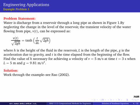
Problem Statement:
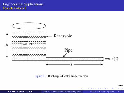
Water is discharge from a reservoir through a long pipe as shown in Figure 1.By
neglecting the change in the level of the reservoir, the transient velocity of the water
flowing from pipe, v(t), can be expressed as:
v(t)p
2gh= tanh
“ t
2L
p
2gh”
where h is the height of the fluid in the reservoir, L is the length of the pipe, g is the
acceleration due to gravity, and t is the time elapsed from the beginning of the flow.
Find the value of h necessary for achieving a velocity of v = 5 m/s at time t = 3 s when
L = 5 m and g = 9.81 m/s2.
Solution:
Work through the example–see Rao (2002).
abu.hasan.abdullah�dev.null MMJ 1113 Computational Methods for Engineers Solution of Nonlinear Equations 4 / 32
Engineering ApplicationsExample Problem 1
Figure 1 : Discharge of water from reservoir.abu.hasan.abdullah�dev.null MMJ 1113 Computational Methods for Engineers Solution of Nonlinear Equations 5 / 32
Engineering ApplicationsExample Problem 2
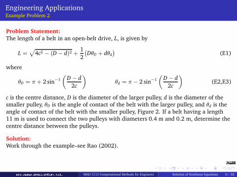
Problem Statement:
The length of a belt in an open-belt drive, L, is given by
L =p
4c2 − (D − d)2 +1
2
`DθD + dθd
´(E1)
where
θD = π + 2 sin−1
„D − d
2c
«
θd = π − 2 sin−1
„D − d
2c
«
(E2,E3)
c is the centre distance, D is the diameter of the larger pulley, d is the diameter of the
smaller pulley, θD is the angle of contact of the belt with the larger pulley, and θd is the
angle of contact of the belt with the smaller pulley, Figure 2. If a belt having a length
11 m is used to connect the two pulleys with diameters 0.4 m and 0.2 m, determine the
centre distance between the pulleys.
Solution:
Work through the example–see Rao (2002).abu.hasan.abdullah�dev.null MMJ 1113 Computational Methods for Engineers Solution of Nonlinear Equations 6 / 32

Engineering ApplicationsExample Problem 2
Figure 2 : Open belt drive.abu.hasan.abdullah�dev.null MMJ 1113 Computational Methods for Engineers Solution of Nonlinear Equations 7 / 32
Engineering ApplicationsExample Problem 3
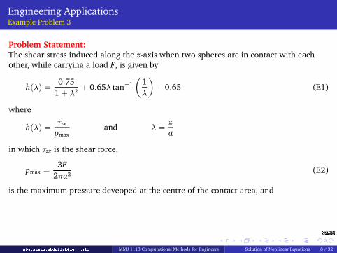
Problem Statement:
The shear stress induced along the z-axis when two spheres are in contact with each
other, while carrying a load F, is given by
h(λ) =0.75
1 + λ2+ 0.65λ tan
−1
„1
λ
«
− 0.65 (E1)
where
h(λ) =τzx
pmaxand λ =
z
a
in which τzx is the shear force,
pmax =3F
2πa2(E2)
is the maximum pressure deveoped at the centre of the contact area, and
abu.hasan.abdullah�dev.null MMJ 1113 Computational Methods for Engineers Solution of Nonlinear Equations 8 / 32
Engineering ApplicationsExample Problem 3
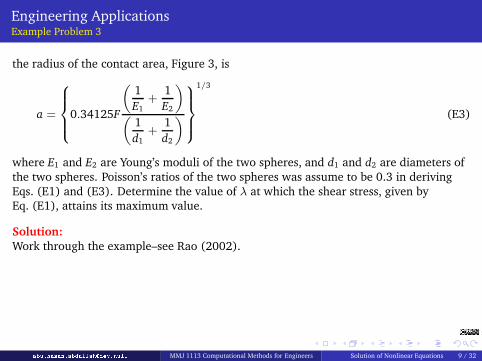
the radius of the contact area, Figure 3, is
a =
8
>><
>>:
0.34125F
„1
E1+
1
E2
«
„1
d1+
1
d2
«
9
>>=
>>;
1/3
(E3)
where E1 and E2 are Young’s moduli of the two spheres, and d1 and d2 are diameters of
the two spheres. Poisson’s ratios of the two spheres was assume to be 0.3 in deriving
Eqs. (E1) and (E3). Determine the value of λ at which the shear stress, given by
Eq. (E1), attains its maximum value.
Solution:
Work through the example–see Rao (2002).
abu.hasan.abdullah�dev.null MMJ 1113 Computational Methods for Engineers Solution of Nonlinear Equations 9 / 32
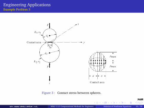
Engineering ApplicationsExample Problem 3
Figure 3 : Contact stress between spheres.abu.hasan.abdullah�dev.null MMJ 1113 Computational Methods for Engineers Solution of Nonlinear Equations 10 / 32
Methods Available
Incremental Search Method
Bisection Method
Newton-Raphson Method
Secant Method
Regula Falsi Method
Fixed Point Iteration Method
Bairstow’ Method
Muller’s Method
abu.hasan.abdullah�dev.null MMJ 1113 Computational Methods for Engineers Solution of Nonlinear Equations 11 / 32
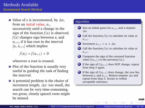
Methods AvailableIncremental Search Method
Value of x is incremented, by ∆x,
from an initial value, x1,
successively until a change in the
sign of the function f(x) is observed.
f(x) changes sign between xi and
xi+1, if it has root in the interval
[xi, xi+1] which implies
f(xi) × f(xi+1) < 0
wherever a root is crossed.
Plot of the function is usually very
useful in guiding the task of finding
the interval.
A potential problem is the choice of
increment length, ∆x: too small, the
search can be very time-consuming,
too great, closely spaced roots might
be missed.
Algorithm
1 Sets an initial guess for xi=1, and a stepsize∆x.
2 Call the function f(x) to calculate its value atxi=1.
3 Increment xi+1 = xi + ∆x.
4 Call the function f(x) to calculate its value atxi+1.
5 Compares the sign of the returned functionvalue f(xi+1) to the previous f(xi).
6 If the sign of f(xi+1) does NOT change, repeatfrom Step 3 again.
7 If the sign of f(xi+1) does change, the root liesbetween xi and xi+1. Reduce stepsize ∆x andrepeat from Step 3. Iterate to withinacceptable tolerance.
abu.hasan.abdullah�dev.null MMJ 1113 Computational Methods for Engineers Solution of Nonlinear Equations 12 / 32
Methods AvailableIncremental Search Method–Example 1
Problem Statement:
Find the root of the equation
f(x) =1.5x
(1 + x2)2− 0.65 tan
−1
„1
x
«
+0.65x
1 + x2= 0 (E1)
using the incremental search method with x1 = 0.0 and ∆x(1) = 0.1.
Solution:
Work through the example.
abu.hasan.abdullah�dev.null MMJ 1113 Computational Methods for Engineers Solution of Nonlinear Equations 13 / 32
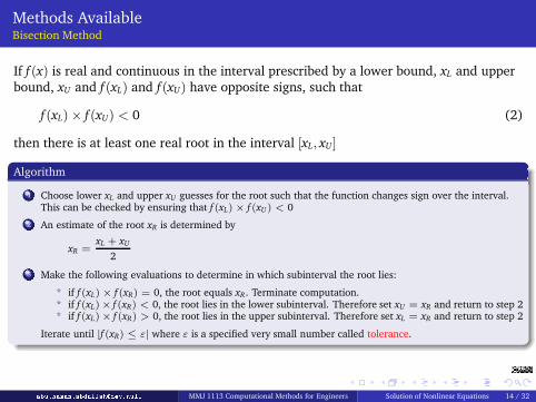
Methods AvailableBisection Method
If f(x) is real and continuous in the interval prescribed by a lower bound, xL and upper
bound, xU and f(xL) and f(xU) have opposite signs, such that
f(xL) × f(xU) < 0 (2)
then there is at least one real root in the interval [xL, xU]
Algorithm
1 Choose lower xL and upper xU guesses for the root such that the function changes sign over the interval.This can be checked by ensuring that f(xL) × f(xU) < 0
2 An estimate of the root xR is determined by
xR =xL + xU
2
3 Make the following evaluations to determine in which subinterval the root lies:
* if f(xL) × f(xR) = 0, the root equals xR. Terminate computation.* if f(xL)× f(xR) < 0, the root lies in the lower subinterval. Therefore set xU = xR and return to step 2* if f(xL) × f(xR) > 0, the root lies in the upper subinterval. Therefore set xL = xR and return to step 2
Iterate until |f(xR) ≤ ε| where ε is a specified very small number called tolerance.abu.hasan.abdullah�dev.null MMJ 1113 Computational Methods for Engineers Solution of Nonlinear Equations 14 / 32
Methods AvailableBisection Method–Example 1
Problem Statement:
Find the root of the equation
f(x) =1.5x
(1 + x2)2− 0.65 tan
−1
„1
x
«
+0.65x
1 + x2= 0 (E1)
using the bisection method with x(1)l = 0.0, x
(1)u = 2.0 and ε = 0.005.
Solution:
Modify the Fortran code, ex1s31.f, and Matlab code , bise t.m, to solve Eq. (E1)
above.
abu.hasan.abdullah�dev.null MMJ 1113 Computational Methods for Engineers Solution of Nonlinear Equations 15 / 32
Methods AvailableNewton-Raphson Method
Function f(x) is expressed using Taylor’s series about an arbitrary point, x1
f(x) = f(x1) + (x − x1)f′(x1) +
1
2!(x − x1)
2f ′′(x1) + . . . (3)
where f , f ′, f ′′, . . . are evaluated at x1
Consider only the first two terms in the expansion
f(x) = f(x1) + (x − x1)f′(x1) = 0 (4)
and set f(x) = 0 to give
f(x1) + (x − x1)f′(x1) = 0 (5)
abu.hasan.abdullah�dev.null MMJ 1113 Computational Methods for Engineers Solution of Nonlinear Equations 16 / 32
Methods AvailableNewton-Raphson Method
Since higher order derivative terms were neglected in the approximation of f(x) in
Eq. (4), the solution of Eq. (5) yields the next approximation to the root (instead of
the exact root) as
x = x2 = x1 −f(x1)
f ′(x1)(6)
x2 denotes improved approximation to the root. For the next improvement we use
x2 in place of x1 on the RHS of Eq. (6) to obtain x3
The iterative procedure of Newton-Raphson method is generalized as
xi+1 = xi −f(xi)
f ′(xi): i = 1, 2, . . . (7)
abu.hasan.abdullah�dev.null MMJ 1113 Computational Methods for Engineers Solution of Nonlinear Equations 17 / 32
Methods AvailableNewton-Raphson Method–Example 1
Problem Statement:
Find the root of the equation
f(x) =1.5x
(1 + x2)2− 0.65 tan
−1
„1
x
«
+0.65x
1 + x2= 0 (E1)
using the Newton-Raphson method with the starting point x1 = 0.0 and the
convergence criteria ε = 10−5.
Solution:
Modify the Fortran code, ex1s32.f, and Matlab code, newton.m, to solve Eq. (E1)
above.
abu.hasan.abdullah�dev.null MMJ 1113 Computational Methods for Engineers Solution of Nonlinear Equations 18 / 32
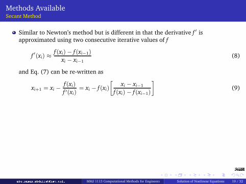
Methods AvailableSecant Method
Similar to Newton’s method but is different in that the derivative f ′ is
approximated using two consecutive iterative values of f
f ′(xi) ≈f(xi) − f(xi−1)
xi − xi−1
(8)
and Eq. (7) can be re-written as
xi+1 = xi −f(xi)
f ′(xi)= xi − f(xi)
»xi − xi−1
f(xi) − f(xi−1)
–
(9)
abu.hasan.abdullah�dev.null MMJ 1113 Computational Methods for Engineers Solution of Nonlinear Equations 19 / 32
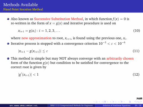
Methods AvailableFixed Point Iteration Method
Also known as Successive Substitution Method, in which function f(x) = 0 is
re-written in the form of x = g(x) and iterative procedure is used on
xi+1 = g(xi) : i = 1, 2, 3, . . . (10)
where new approximation to root, xi+1, is found using the previous one, xi.
Iterative process is stopped with a convergence criterion 10−3 < ε < 10−6
|xi+1 − g(xi+1)| ≤ ε (11)
This method is simple but may NOT always converge with an arbitrarily chosen
form of the function g(x) but condition to be satisfied for convergence to the
correct root is given by
|g′(xi+1)| < 1 (12)
abu.hasan.abdullah�dev.null MMJ 1113 Computational Methods for Engineers Solution of Nonlinear Equations 20 / 32
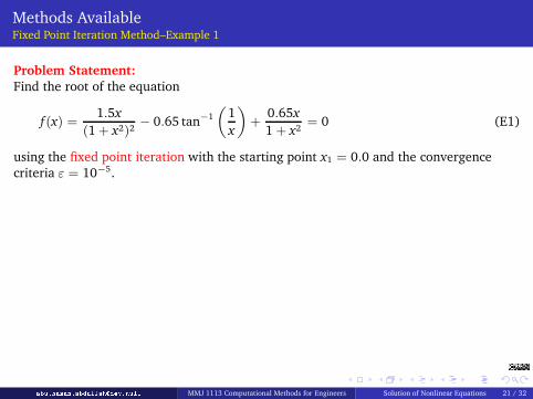
Methods AvailableFixed Point Iteration Method–Example 1
Problem Statement:
Find the root of the equation
f(x) =1.5x
(1 + x2)2− 0.65 tan
−1
„1
x
«
+0.65x
1 + x2= 0 (E1)
using the fixed point iteration with the starting point x1 = 0.0 and the convergence
criteria ε = 10−5.
abu.hasan.abdullah�dev.null MMJ 1113 Computational Methods for Engineers Solution of Nonlinear Equations 21 / 32
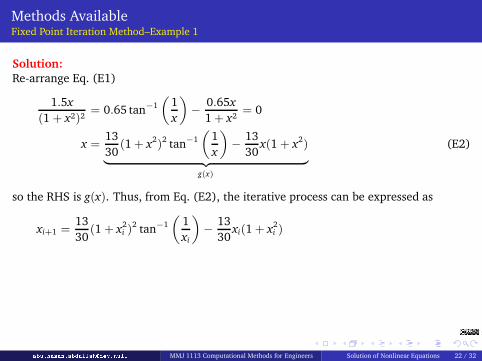
Methods AvailableFixed Point Iteration Method–Example 1
Solution:
Re-arrange Eq. (E1)
1.5x
(1 + x2)2= 0.65 tan
−1
„1
x
«
−0.65x
1 + x2= 0
x =13
30(1 + x
2)2tan
−1
„1
x
«
−13
30x(1 + x
2)
| {z }
g(x)
(E2)
so the RHS is g(x). Thus, from Eq. (E2), the iterative process can be expressed as
xi+1 =13
30(1 + x
2i )
2tan
−1
„1
xi
«
−13
30xi(1 + x
2i )
abu.hasan.abdullah�dev.null MMJ 1113 Computational Methods for Engineers Solution of Nonlinear Equations 22 / 32

Root Finding with MatlabExample 1
Problem Statement:
Find the root of the equation
f(x) = tan−1
x = 0
using Matlab.
Solution:
Matlab Codex = -2*pi:0.01:2*pi;fx = 'atan(x)';fplot(fx,[-2*pi 2*pi℄)xlabel('x'),ylabel('y=f(x)'),title('Root Finding')root = fzero(fx,1.6)abu.hasan.abdullah�dev.null MMJ 1113 Computational Methods for Engineers Solution of Nonlinear Equations 23 / 32
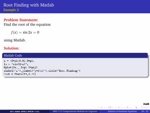
Root Finding with MatlabExample 2
Problem Statement:
Find the root of the equation
f(x) = sin 2x = 0
using Matlab.
Solution:
Matlab Codex = -2*pi:0.01:2*pi;fx = 'sin(2*x)';fplot(fx,[-2*pi 2*pi℄)xlabel('x'),ylabel('y=f(x)'),title('Root Finding')root = fzero(fx,0.75)abu.hasan.abdullah�dev.null MMJ 1113 Computational Methods for Engineers Solution of Nonlinear Equations 24 / 32
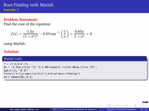
Root Finding with MatlabExample 3
Problem Statement:
Find the root of the equation
f(x) =1.5x
(1 + x2)2− 0.65 tan
−1
„1
x
«
+0.65x
1 + x2= 0
using Matlab.
Solution:
Matlab Codex = -2.0:0.01:2;fx = '1.5*x./(1+x.^2).^2-0.65*(atan(1./x))+0.65*x./(1+x.^2)';fplot(fx,[-2 2℄)xlabel('x'),ylabel('y=f(x)'),title('Root Finding')x2 = fzero(fx,-0.1)abu.hasan.abdullah�dev.null MMJ 1113 Computational Methods for Engineers Solution of Nonlinear Equations 25 / 32
Roots of Nonlinear Polynomials
There is theorem which states that there is no such formula for general
polynomials of degree higher than four.
In practice we use numerical method to solve polynomial equations of degree
higher than two.
As a special case of f(x) = 0, consider a polynomial equation
f(x) = anxn + an−1x
n−1 + . . . + a2x2 + a1x + a0 = 0 (13)
where n denote degree of polynomial, a0, a1, a2 . . . an are coefficients of
polynomial. Eq. (13) in general will have n roots
abu.hasan.abdullah�dev.null MMJ 1113 Computational Methods for Engineers Solution of Nonlinear Equations 26 / 32
Roots of Nonlinear Polynomials
If x1, x2 . . . xn are roots of Eq. (13), they are related to the coefficients ofpolynomial as
nX
i=1
xi = −
an−1
an
nX
i=1
xi
nX
j=1,j6=1
xixj = −
an−2
an
nX
i=1
xi
nX
j=1,j6=i
nX
k=1,k 6=j
xixjxk = −
an−3
an
. . .
x1x2 . . . xn−1xn = (−1)n a0
an(14)
abu.hasan.abdullah�dev.null MMJ 1113 Computational Methods for Engineers Solution of Nonlinear Equations 27 / 32
Roots of Nonlinear PolynomialsMuller’s Method
Your homework!
Read Section 7.4, pp 167–171 of STEVEN C. CHAPRA, RAYMOND P. CANALE (2006): Numerical Methods for Engineers, 5ed,ISBN 007-124429-8, McGraw-Hill
Read Section 2.11, pp. 84–88 of SINGIRESU S. RAO (2002): Applied Numerical Methods for Engineers and Scientists, ISBN0-13-089480-X, Prentice Hall
abu.hasan.abdullah�dev.null MMJ 1113 Computational Methods for Engineers Solution of Nonlinear Equations 28 / 32
Roots of Nonlinear PolynomialsExample 1
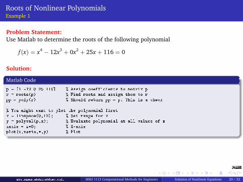
Problem Statement:
Use Matlab to determine the roots of the following polynomial
f(x) = x4 − 12x
3 + 0x2 + 25x + 116 = 0
Solution:
Matlab Codep = [1 -12 0 25 116℄ % Assign oeffi ients to matrix pr = roots(p) % Find roots and assign them to rpp = poly(r) % Should return pp = p. This is a he k% You might want to plot the polynomial firstx = linspa e(0,12); % Set range for xy = polyval(p,x); % Evaluate polynomial at all values of xxaxis = x*0; % X-axisplot(x,xaxis,x,y) % Plotabu.hasan.abdullah�dev.null MMJ 1113 Computational Methods for Engineers Solution of Nonlinear Equations 29 / 32
Roots of Nonlinear PolynomialsExample 2
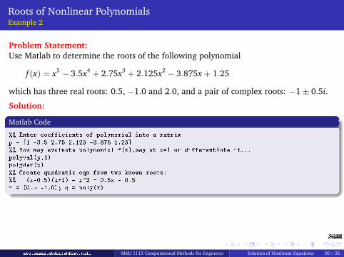
Problem Statement:
Use Matlab to determine the roots of the following polynomial
f(x) = x5 − 3.5x
4 + 2.75x3 + 2.125x
2 − 3.875x + 1.25
which has three real roots: 0.5, −1.0 and 2.0, and a pair of complex roots: −1 ± 0.5i.
Solution:
Matlab Code%% Enter oeffi ients of polynomial into a matrixp = [1 -3.5 2.75 2.125 -3.875 1.25℄%% You may evaluate polynomial f(x),say at x=1 or differentiate it...polyval(p,1)polyder(p)%% Create quadrati eqn from two known roots:%% (x-0.5)(x+1) = x^2 + 0.5x - 0.5r = [0.5 -1.0℄; q = poly(r)abu.hasan.abdullah�dev.null MMJ 1113 Computational Methods for Engineers Solution of Nonlinear Equations 30 / 32
Roots of Nonlinear PolynomialsExample 2
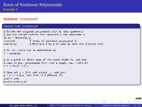
Solution: (continued)
Matlab Code (continued)% Divide the original polynomial f(x) by this quadrati % eqn and assign results into quotient d and remainder e[d e℄ = de onv(p,q)roots(d) % Roots of quotient polynomial d onv(d,q) % Multiply d by q to ome up with the original f(x)% Or, ALL roots may be determined byr = roots(p)% As a guide to where some of its roots might be, you may% want to plot polynomial f(x) over a range, say, -10<x<10x = [-10:0.1:10℄;% Then set y = f(x) and x-axis ... and ploty = x.^4-3.5*x.^3+2.75*x.^2-3.875*x+1.25;yis0 = x*0;plot(x,yis0,x,y)abu.hasan.abdullah�dev.null MMJ 1113 Computational Methods for Engineers Solution of Nonlinear Equations 31 / 32
Bibliography
1 SINGIRESU S. RAO (2002): Applied Numerical Methods for Engineers and Scientists, ISBN0-13-089480-X, Prentice Hall
2 STEVEN C. CHAPRA, RAYMOND P. CANALE (2006): Numerical Methods for Engineers, 5ed,ISBN 007-124429-8, McGraw-Hill
3 DAVID KINCAID AND WARD CHENEY (1991): Numerical Analysis: Mathematics of ScientificComputing, ISBN 0-534-13014-3, Brooks/Cole Publishing Co.
4 STEVEN C. CHAPRA (2005): Applied Numerical Methods with MATLAB for Engineers andScientists, ISBN 007-124484-0, McGraw-Hill
5 WILLIAM J. PALM III (2005): Introduction to Matlab 7 for Engineers, ISBN 007-123262-1,McGraw-Hill
6 JOHN D. ANDERSON, JR. (1995): Computational Fluid Dynamics–The Basics withApplications, ISBN 007-113210-4, McGraw-Hill
abu.hasan.abdullah�dev.null MMJ 1113 Computational Methods for Engineers Solution of Nonlinear Equations 32 / 32
Top Related