


Languages
Pages
Legal


Missile longitudinal autopilot design using a newsuboptimal nonlinear control method
M. Xin and S.N. Balakrishnan
Abstract: A missile longitudinal autopilot is designed using a new nonlinear control synthesistechnique called the u–D approximation. The particular u–D methodology used is referred to asthe u–D H2 design. The technique can achieve suboptimal closed-form solutions to a class ofnonlinear optimal control problems in the sense that it solves the Hamilton–Jacobi–Bellmanequation approximately by adding perturbations to the cost function. An interesting feature of thismethod is that the expansion terms in the expression for suboptimal control are nothing butsolutions to the state-dependent Riccati equations associated with this class of problems. The u–DH2 design has the same structure as that of the linear H2 formulation except that the two Riccatiequations are state dependent. Numerical simulations are presented that demonstrate the potentialof this technique for use in an autopilot design. These results are compared with the recentlypopular SDRE H2 method.
1 Introduction
Modern aircraft or missiles often operate in flight regimeswhere nonlinearities significantly affect dynamic response.For example, a high-performance missile must be quicklyresponsive to and follow accurately any guidance com-mands, so that it can intercept fast moving and agile targets.Many nonlinear control methods have been proposed for themissile autopilot design. One popular method of formulationhas been the optimal control of nonlinear dynamics withrespect to a mathematical index of performance [1]. A majordifficulty in this line of approach is finding solutions to theresulting Hamilton–Jacobi–Bellman (HJB) equation.
Suboptimal solutions are found by power series expan-sion methods. Wernli and Cook [2] developed an approachby bringing the original system into an apparent linear form.Their suboptimal control involves finding the Taylorexpansion of the solution to a state-dependent Riccatiequation. But the convergence of this series is notguaranteed and the resulting control law leads to largecontrol efforts when the initial states are large. Garrard [3, 4]formulated another approach that expanded both the optimalcost and the nonlinear dynamics as power series of the statesand employed it in the high-angle-of-attack maneuverableaircraft. However, this method has to assume the structureof the optimal cost as a scalar polynomial with undeter-mined coefficients which contains all possible combinationsof products of the elements of the state vector. As the systemorder increases, the complexity of determining thesecoefficients increases dramatically. The common problemwith these methods is that they do not offer a way to ensurethat the system is asymptotically stable in the large.
Beard et al. [5] adopted the Galerkin approximation tosolve the HJB equation. It was used to synthesise anonlinear optimal control for a missile autopilot system[6]. The control laws are given as a series of basis functions.To find an admissible control to satisfy all the ten conditionsproposed in that paper is not an easy task.
Another recently emerging technique that systematicallysolves the nonlinear regulator problem is the state-dependent Riccati equation (SDRE) method [7]. By turningthe equations of motion into a linear-like structure, thisapproach permits the designer to employ linear optimalcontrol methods such as the LQR methodology and the H1design technique for the synthesis of nonlinear controlsystems. The SDRE method however, needs onlinecomputations of the algebraic Riccati equation at eachsample time.
A new suboptimal nonlinear controller synthesis (�–Dapproximation) technique based on approximate solution tothe Hamilton–Jacobi–Bellman equation is proposed in thispaper. By introducing an artificial variable �; the costate lcan be expanded as a power series in terms of �: Thistechnique can overcome the problem of large-control-for-large-initial-states encountered by using the control law in[2]. By adjusting some perturbation parameters in the costfunction, we are also able to modulate the transientperformance of the system.
We extend the standard linear H2 optimal control methodto nonlinear problems using the �–D technique. The linearH2 control problem has been studied and implemented since1960s [8]. It is used to find a proper controller that stabilisesthe system internally and minimise the H2 norm of thetransfer function from the exogenous input to the perform-ance output. With output feedback, the H2 design ends upwith having to solve two Riccati equations. Some studiesexamined the use of H2 controller design in nonlinearsystems. In [9], the SDRE H2 method was used to design afull-envelope pitch autopilot. However, solving two Riccatiequations online is very timeconsuming. In this paper, �–DH2 design is proposed for the same problem as that in [9]that gives an approximate closed-form solution to the twostate-dependent Riccati equations.
q IEE, 2003
IEE Proceedings online no. 20030966
doi: 10.1049/ip-cta:20030966
The authors are with the Department of Mechanical and AerospaceEngineering and Engineering Mechanics, University of Missouri-Rolla,Rolla, MO 65401, USA
Paper first received 23rd October 2002 and in revised form 29th July 2003
IEE Proc.-Control Theory Appl., Vol. 150, No. 6, November 2003 577
2 Suboptimal control of a class of nonlinearsystems
We consider systems described by
_xx ¼ f ðxÞ þ BðxÞu ð1Þ
The problem is to find the control u(t) which minimises thecost J given by
J ¼ 1
2
Z 1
0ðxT Qx þ uT RuÞdt ð2Þ
where x 2 O � Rn; f :O ! Rn; B 2 Rnm; u :O ! Rm; Q 2Rnn; R 2 Rmm; O is a compact set in Rn; Q is positivesemidefinite matrix and R is positive definite matrix; fð0Þ ¼0: The solution to (2) is obtained by solving the Hamilton–Jacobi–Bellman partial differential equation [1]
@VT
@xf ðxÞ 1
2
@VT
@xBðxÞR1BTðxÞ @V
@xþ 1
2xT Qx ¼ 0 ð3Þ
with Vð0Þ ¼ 0: The optimal control is given by
u ¼ R1BTðxÞ @V
@xð4Þ
and V(x) is the optimal cost, i.e.
VðxÞ ¼ minu
1
2
Z 1
0ðxT Qx þ uT RuÞdt ð5Þ
The HJB equation is extremely difficult to solve in general;in this study we find approximate solutions. Add pertur-bations to the cost function as
J ¼ 1
2
Z 1
0xT Q þ
X1i¼1
Di�i
!x þ uT Ru
" #dt
ð6Þ
where � and Di are chosen such that Q þP1
i¼1 Di�i is
positive semidefinite. For later use we rewrite the state
equation as
_xx ¼ f ðxÞ þ BðxÞu
¼ A0 þ �AðxÞ�
� �x þ g0 þ �
gðxÞ�
� �u
ð7Þ
where A0 is a constant matrix such that ðA0; g0Þ is astabilisable pair and ½ðA0 þ AðxÞÞ; ðg0 þ gðxÞÞ� is pointwisecontrollable. Define
l ¼ @V
@xð8Þ
By using (8) in (3) we have
lT f ðxÞ 1
2lT BðxÞR1BTðxÞlþ 1
2xT Q þ
X1i¼1
Di�i
!x ¼ 0
ð9Þ
Assume a power series expansion of l as
l ¼X1i¼0
Ti�ix ð10Þ
where Ti are to be determined and assumed to be symmetric.By substituting (10) into (3) and equating the coefficients ofpowers of � to zero we get
T0A0 þ AT0 T0 T0g0R1gT
0 T0 þ Q ¼ 0 ð11Þ
T1ðA0 g0R1gT0 T0Þ þ ðAT
0 T0g0R1gT0 ÞT1
¼ T0AðxÞ�
ATðxÞT0
�þ T0g0R1 gT
�T0
þ T0
g
�R1gT
0 T0 D1 ð12Þ
T2ðA0 g0R1gT0 T0Þ þ ðAT
0 T0g0R1gT0 ÞT2
¼ T1AðxÞ�
ATðxÞT1
�þT0g0R1 gT
�T1
þT0
g
�R1gT
0 T1 þT0
g
�R1 gT
�T0 þT1g0R1gT
0 T1
þT1g0R1 gT
�T0 þT1
g
�R1gT
0 T0 D2
ð13Þ
TnðA0g0R1gT0 T0ÞþðAT
0 T0g0R1gT0 ÞTn
¼ Tn1AðxÞ�
ATðxÞTn1
�
þXn1
j¼0
Tj g0R1 gT
�þg
�R1gT
0
� Tn1j
þXn2
j¼0
TjgR1gT Tn2jþXn1
j¼1
Tjg0R1gT0 TnjDn
ð14Þ
Since the right-hand side of (11)–(14) involve x and �;Ti ¼ Tiðx; �Þ: The expression for control can be obtained ina power series as
u ¼ R1BTðxÞl ¼ R1BTðxÞX1i¼0
Tiðx; �Þ�ix ð15Þ
Note that (11) is an algebraic Riccati equation. The rest ofequations are linear Lyapunov equations. In the rest of thispaper we call this method the �–D approximationtechnique. The algorithm in [2] results in the‘�-approximation’ (without the Di terms) although througha different approach. A problem with the �-approximation isthat large initial conditions may give rise to large control oreven instability. We avoid it by constructing Di as
D1 ¼ k1el1t T0AðxÞ�
ATðxÞT0
�
�ð16Þ
D2 ¼ k2el2t T1AðxÞ�
ATðxÞT1
�
�ð17Þ
..
.
Dn ¼ knelnt Tn1AðxÞ�
ATðxÞTn1
�
�ð18Þ
where ki and li > 0; i ¼ 1; n are constants. Themotivation for this kind of Di construction is to offsetthe large control results from the state dependent term A(x)in (11)–(14). For example, when A(x) includes a cubicterm, a higher initial state will result in higher initial Ti
and consequently higher initial control. So if we choose Di
such that
IEE Proc.-Control Theory Appl., Vol. 150, No. 6, November 2003578

Ti1AðxÞ�
ATðxÞTi1
� Di
¼ eiðtÞ Ti1AðxÞ�
ATðxÞTi1
�
�ð19Þ
where eiðtÞ ¼ 1 kielit and eiðtÞ is a small number, ei can
be used to suppress this large value to propagate in(12)–(14). eiðtÞ is chosen to satisfy some conditionsrequired in the proof of convergence and stability of thealgorithm [10] while elit with li > 0 is used to let theperturbation terms in the cost function and HJB equationdiminish with time. ðki; liÞ are design parameters which canbe tuned to adjust system transient performance.
Remark 2.1: Solutions to (11)–(14) are carried out offlinefrom top to bottom. Equation (11) is a standard algebraicRiccati equation. The rest of (12)–(14) are linear equationsin terms of T2; ;Tn with constant coefficients A0 g0R1gT
0 T0 and AT0 T0g0R1gT
0 : So we get the closed-form solutions for T2; ;Tn with just one matrix inverseoperation after some algebra.
Remark 2.2: � is just an intermediate variable. It turns out tobe cancelled by the choice of Di matrices (see (16)–(18)).In the simulation, it is set to one. Theoretical work onconvergence of series expansion of
P1i¼0 Tiðx; �Þ�i; semi-
globally asymptotic stability of the �–D method etc. can befound in [10].
3 Missile longitudinal autopilot design
3.1 Formulation of �– D H2 problem
Consider the general nonlinear system
_xx ¼ f ðxÞ þ BwðxÞw þ BuðxÞu ð20Þ
z ¼ czðxÞ þ DzuðxÞu ð21Þ
y ¼ cyðxÞ þ DywðxÞw ð22Þ
where w is the exogenous input including trackingcommand and noises injected into the system; u is thecontrol, z is the performance output and y is themeasurement output.
The nonlinear dynamic is rewritten to have a linear-likestructure as
_xx ¼ AðxÞx þ BwðxÞw þ BuðxÞu ð23Þ
z ¼ CzðxÞx þ DzuðxÞu ð24Þ
y ¼ CyðxÞx þ DywðxÞw ð25Þ
Then the following formulation is similar to the standardlinear H2 problem except that the coefficent matrices of x, uand w are state-dependent. This has the same formulation asSDRE H2 at this point [9].
The linear H2 problem leads to solving two Riccatiequations given in terms of their hamiltonians
A BuR12 RT
12 BuR12 BT
u
R1 þ R12R12 RT
12 ðA BuR12 RT
12ÞT
�ð26Þ
ðA V12V12 CyÞT CT
y V12 Cy
V1 þ V12V12 VT
12 ðA V12V12 CyÞ
�ð27Þ
where
V1 ¼ BwBTw V12 ¼ BwDT
yw V2 ¼ Dyw DTyw
R1 ¼ CTz Cz R12 ¼ CT
z Dzu R2 ¼ DTzu Dzu ð28Þ
Assume that the solutions to (26) and (27) are P1 and P2:If we rewrite (20)–(22) as linear-like systems (23)–(25),the nonlinear H2 problem needs to solve the state-dependentRiccati equation (26) and (27) where the argument x hasbeen omitted for brevity. Construct the nonlinear feedbackcontroller via
dxx
dt¼ Ac xx þ Bc y ð29Þ
u ¼ Cc xx ð30Þwhere Ac; Bc; and Cc are
Ac ¼ A þ BuCc BcCy ð31Þ
Bc ¼ ½P2CTy þ V12�V1
2 ð32Þ
Cc ¼ R12 ½BT
u P1 þ RT12� ð33Þ
It is interesting to note that solving the state-dependentRiccati equation (26) is equivalent to solving the followingnonlinear optimal control problem:
Find u(t) to minimise J where
J ¼Z 1
0xT ½ðR1 R12R1
2 RT12Þx þ uT R1
2 u�dt ð34Þ
subject to
_xx ¼ ½AðxÞ BuðxÞR12 RT
12�x þ BuðxÞu ¼ f ðxÞ þ BuðxÞuð35Þ
This class of nonlinear optimal control problem can besolved by using the �–D technique. The same is true for thesecond state-dependent Riccati equation (27).
3.2 Missile longitudinal dynamics
The missile model used in this paper is taken from [9]; itassumes constant mass, post burnout, no roll rate, zero rollangle, no sideslip, and no yaw rate. The rigid body equationsof motion reduce to two force equations, one momentequation, and one kinematic equation
_UU þ qW ¼P
FBX
mð36Þ
_WW qU ¼P
FBZ
mð37Þ
_qq ¼P
MY
IY
ð38Þ
_�� ¼ q ð39Þwhere U and W are components of velocity vector V
*
T alongthe body-fixed x- and z-axes; � is the pitch angle; q is thepitch rate about the body y-axis; m is the missile mass. Theforces along the body–fixed co-ordinates and moments
IEE Proc.-Control Theory Appl., Vol. 150, No. 6, November 2003 579

about the centre of gravity are shown in Fig. 1. The forceand moments about the centre of gravity areX
FBX¼ L sin a D cos a mg sin � ð40Þ
XFBZ
¼ L cos a D sin aþ mg cos � ð41Þ
XMY ¼ �MM ð42Þ
where a is angle of attack; L denotes lift; D denotes drag and�MM is the pitching moment.
L ¼ 1
2rV2SCL; D ¼ 1
2rV2SCD; �MM ¼ 1
2rV2SdCm ð43Þ
The normal force coefficient CZ is used to calculate the liftand drag coefficients
CL ¼ CZ cos a; CD ¼ CD0 CZ sin a ð44Þ
where CD0is the drag coefficient at the zero angle of attack.
The nondimensional aerodynamic coefficients at 6096maltitude are:
CZ ¼ ana3 þ bnajaj þ cn 2 M
3
� aþ dnd ð45Þ
Cm ¼ ama3 þ bmajaj þ cm 7 þ 8M
3
� aþ dmdþ emq
ð46Þ
In this paper we adopt Mach number M, angle of attack a;flight path angle g; and pitch rate q as the states since theyappear in the aerodynamic coefficients. Note that
tan a ¼ W
U; V2 ¼ U2 þ W2; M ¼ V
a; g ¼ � a ð47Þ
and
_MM ¼_VV
a; _VV ¼
_UUU þ _WWW
Vð48Þ
The numerical values for the coefficients in (45) and (46) aregiven in Table 1 and the physical parameters associated withthis missile are given in Table 2.
The state equations can now be written as
_MM ¼ 0:7P0S
ma½M2ðCD0
CZ sin a� g
asin g ð49Þ
_aa ¼ 0:7P0S
maMCZ cos aþ
g
aMcos gþ q ð50Þ
_gg ¼ 0:7P0S
maMCZ cos a
g
aMcos g ð51Þ
_qq ¼ 0:7P0Sd
IY
M2Cm ð52Þ
By substituting the aerodynamic data, (49)–(52) become
_MM ¼ 0:4008M2a3 sin a 0:6419M2jaja sin a
0:2010M2 2 M
3
� a sin a 0:0062M2
0:0403M2 sin ad 0:0311 sin g ð53Þ
_aa ¼ 0:4008Ma3 cos a 0:6419Mjaja cos a
0:2010M 2 M
3
� a cos a
0:0403M cos ad 0:0311cos g
Mþ q ð54Þ
_gg ¼ 0:4008Ma3 cos aþ 0:6419Mjaja cos a
þ 0:2010M 2 M
3
� a cos a
þ 0:0403M cos adþ 0:0311cos g
M ð55Þ
_qq ¼ 49:82M2a3 78:86M2jaja
þ 3:60M2 7 þ 8M
3
� a
14:54M2d 2:12M2q ð56Þ
Actuator dynamics are incorporated with the followingdynamics:
_dd€dd
�¼ 0 1
o2a 2zoa
�d_dd
�þ 0
o2a
�dc ð57Þ
where z ¼ 0:7 and oa ¼ 50: The normal acceleration (in gs)is described by
Table 2: Physical Parameters
Symbol Name Value
P0 Static Pressure 973:3 lb=ft2
IY Moment of Inertia 182:5 slug � ft2
S Reference Area 0:44 ft2
d Reference Distance 0:75 ft
m Mass 13:98 slug
a Speed of Sound 1036:4 ft= sec
g Gravity 32:2 ft= sec2
Table 1: Aerodynamic Coefficients
Force Moment
an ¼ 19:373 am ¼ 40:440
bn ¼ �31:023 bm ¼ �64:015
cn ¼ �9:717 cm ¼ 2:922
dn ¼ �1:948 dm ¼ �11:803
CD0¼ 0:300 em ¼ �1:719
VTγα θ
MY
CL L
D
FBZ CZ
FBX
W
U
horizontal reference
mg
body z-axis
body x-axis
Fig. 1 Longitudinal forces and moment acting on missile
IEE Proc.-Control Theory Appl., Vol. 150, No. 6, November 2003580

nz ¼P
FBZ
mgþ cos � ¼ 0:7P0S
mgM2CZ þ cosðgþ aÞ ð58Þ
In terms of the flight conditions at 6096m,
nz ¼ 12:901M2a3 20:659M2jaja
6:471M2 2 M
3
� a
1:297M2dþ cosðgþ aÞ ð59Þ
3.3 �– D controller design
The controller objective is to drive the system to track thecommanded normal acceleration (in gs). The tracking blockdiagram is shown in Fig. 2. The Kalman gain K1 and K2 arethe solutions of the dynamic feedback controller (29)–(33).The control weight is rc: The plant and output disturbanceweights are rw and rD: The performance weighting functionfor tracking error yr ym is chosen to be [9]
WtðsÞ ¼1
s þ 0:001ð60Þ
or in state-space form
Wt ¼At Bt
Ct 0
264
375 ¼ 0:001 1
1 0
�ð61Þ
Performance output is
z ¼ zt zc½ �T ð62ÞThe augmented state-space x is given as
x ¼ ½M; a; g; q; d; _dd; xt�T ð63ÞThe control variable is the fin deflection
u ¼ dc ð64ÞThe measurement vector is
ym ¼ nz M q½ �T ð65ÞThe acceleration command
yr ¼ nzcð66Þ
where nzcis the normal acceleration command. So the
output vector in the controller design is
y ¼ yr ym½ �T¼ nzcym
� �T¼ nzcnz M q
� �T ð67Þ
The exogenous input is
w ¼ nzcDplant Dnz
DM Dq
� �T ð68Þ
where Dplant is the process noise and ½DnZDM Dq�T the
measurement noise. In the simulation they are assumedgaussian with unit variance.
The plant noise weights are chosen to be:
rw ¼ 0:2 0:01 0:01 0:2 0:01 0:01½ �T ð69ÞThe measurement noise weights on nz; M and q are,respectively, the diagonal elements of
rD ¼0:01 0 0
0 0:001 0
0 0 0:01
24
35
ð70ÞTo avoid overflow in the numerical simulations, sin g=g isset to 1 when g is less than 104 radian.
In the �–D formulation we choose the partition of (7) as
_xx ¼ Aðx0Þ þ �AðxÞ Aðx0Þ
�
� �x
þ Bðx0Þ þ �BðxÞ Bðx0Þ
�
� �u
ð71ÞThe advantage of choosing this partition is that in the �–Dformulation T0 is solved from A0 and g0 in (7) and (11).If A0 ¼ Aðx0Þ and g0 ¼ Bðx0Þ are selected, one would havea good starting point for T0 because Aðx0Þ and Bðx0Þ keepmuch more system information than an arbitrary choice ofA0 and g0:
4 Numerical results and analysis
The simulation scenario is to initially command a zero-gnormal acceleration, a square wave of magnitude 10g at onesecond, returning to zero at three seconds. The initial statespace is x0 ¼ ½2:5 0 0 0 0 0 0�T :The simulation isrun at 100 Hz. In solving the two state-dependent Riccatiequations (26) and (27), we use T0; T1 and T2 terms in thel expansion (10). Three terms have been found to besufficient. For comparison we also use the SDRE H2 method.
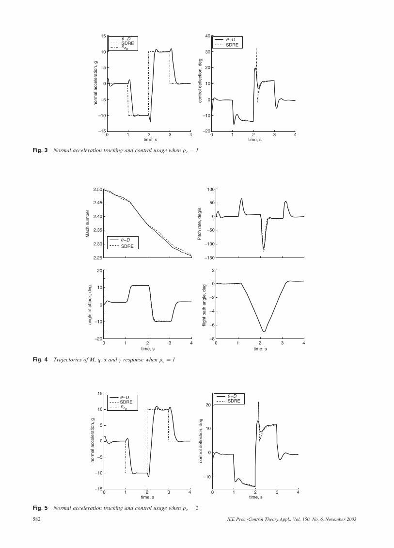
The results are presented in Figs. 3–9. Figure 3 showsthe commanded and achieved normal acceleration
yr = nzc K1 + Bu(x)
rc
zc
∫ C(x)
A(x)
K2
+
Wt
–
ym+ +
+
∆q
∆M
∆nz
+ + +
∆plant
zt
rw r∆
Fig. 2 H2 tracking block diagram
IEE Proc.-Control Theory Appl., Vol. 150, No. 6, November 2003 581
Mac
h nu
mbe
r
2.25
2.30
2.35
2.40
2.45
2.50
SDRE
Pitc
h ra
te, d
eg/s
–150
–100
–50
0
50
100
0
angl
e of
atta
ck, d
eg
–20
–10
0
10
20
1 2 3 4time, s
0
fligh
t pat
h an
gle,
deg
–8
–6
–4
–2
0
2
1 2 3 4time, s
q –D
Fig. 4 Trajectories of M, q, a and g response when rc ¼ 1
0
SDREnzc
norm
al a
ccel
erat
ion,
g
–15
–10
–5
0
5
10
15
1 2 3 4time, s
0
SDRE
cont
rol d
efle
ctio
n, d
eg
–10
0
10
20
1 2 3 4time, s
q –D q –D
Fig. 5 Normal acceleration tracking and control usage when rc ¼ 2
0
norm
al a
ccel
erat
ion,
g
1 2 3 4time, s
–15
–10
–5
0
5
10
q –D q –DSDREnzc
15
0
cont
rol d
efle
ctio
n, d
eg
1 2 3 4time, s
–20
–10
0
10
20
30
SDRE
40
Fig. 3 Normal acceleration tracking and control usage when rc ¼ 1
IEE Proc.-Control Theory Appl., Vol. 150, No. 6, November 2003582

and the control usage when the weight rc of control is 1.Both the SDRE method and the �–D method track very welland have reasonable transient responses. Figure 4 shows thatthe state histories are similar for both methods. The normal
acceleration tracking for SDRE has no overshoot and a littlefaster response. However, it needs considerable controleffort at this jump as seen from Fig. 4. Figure 5 representsthe effects of increase in the control weight rc to 2. While
0
norm
al a
ccel
erat
ion,
g
–15
–10
–5
0
5
10
15
1 2 3 4time, s
0
cont
rol d
efle
ctio
n, d
eg
–10
0
10
20
30
60
1 2 3 4time, s
Fig. 7 Normal acceleration tracking and control usage with rc ¼ 1 and with Di added
0
commandk1 = k2 = 0.9, t1 = t2 = 1
k1 = k2 = 0.9, t1 = t2 = 40
norm
al a
ccel
erat
ion,
g
–15
–10
–5
0
5
10
15
1 2 3 4time, s
0
cont
rol d
efle
ctio
n, d
eg
–10
–20
0
10
20
30
40
1 2 3 4time, s
k1 = k2 = 0.9, t1 = t2 = 1
k1 = k2 = 0.9, t1 = t2 = 40
Fig. 8 Normal acceleration tracking and control usage with rc ¼ 1 and with different ðki; liÞ
0
norm
al a
ccel
erat
ion,
g
–15
–10
–5
0
5
10
15
1 2 3 4time, s
0
cont
rol d
efle
ctio
n, d
eg
–10
0
10
20
30
60
1 2 3 4time, s
Fig. 6 Normal acceleration tracking and control usage with rc ¼ 1 and without Di
IEE Proc.-Control Theory Appl., Vol. 150, No. 6, November 2003 583
the control usage is reduced, the normal accelerationtracking shows more lag and overshoot.
As discussed in Section 2, the construction of pertur-bation matrices Di in (16)–(19) is used to overcome theinitial large control problem which is induced by thepropagation of large initial states through �–D algorithm(11)–(14). The �–D design parameters are chosen as
D1 ¼ e40t T0 AðxÞ�
ATðxÞT0
�
�;
D2 ¼ e40t T1AðxÞ�
ATðxÞT1
�
�ð72Þ
These parameters are selected based on many initialconditions of interest. For the initial state x0 ¼ ½2:5 0 0 00 0 0�T ; the tracking is good and the control usage isreasonable even without D1 and D2: To demonstrate thefunction of D1 and D2; the results from a different initialstate x0 ¼ ½3:5 50 50 100=s 0 0 0�T is given in Figs. 6 and 7.As can be seen from Fig. 6, the initial maximum control isabout 580 without D1 and D2 but is reduced to 290 with D1
and D2 in Fig. 7. The selection of ðki; liÞ in Di terms isproblem dependent. A large exponential parameter ischosen in this particular problem because we found thatlarge control only happens at the very early stage. It may notbe the case for other problems in which ðki; liÞ could besmall values. These are design parameters that need tuning.Numerical experiments with these parameters show that thesystem performance is not sensitive to the variations aroundthe selected values. To show this, Fig. 8 presents the resultswith two other sets of parameters k1 ¼ k2 ¼ 0:9; l1 ¼ l2 ¼40 and k1 ¼ k2 ¼ 0:9; l1 ¼ l2 ¼ 1: As can be seen, thetracking performance does not change significantly and themaximum control effort for both cases is about 370:Compared with large l1 ¼ l2 ¼ 40; the transient responsein the first second with l1 ¼ l2 ¼ 1 is only a little worse.
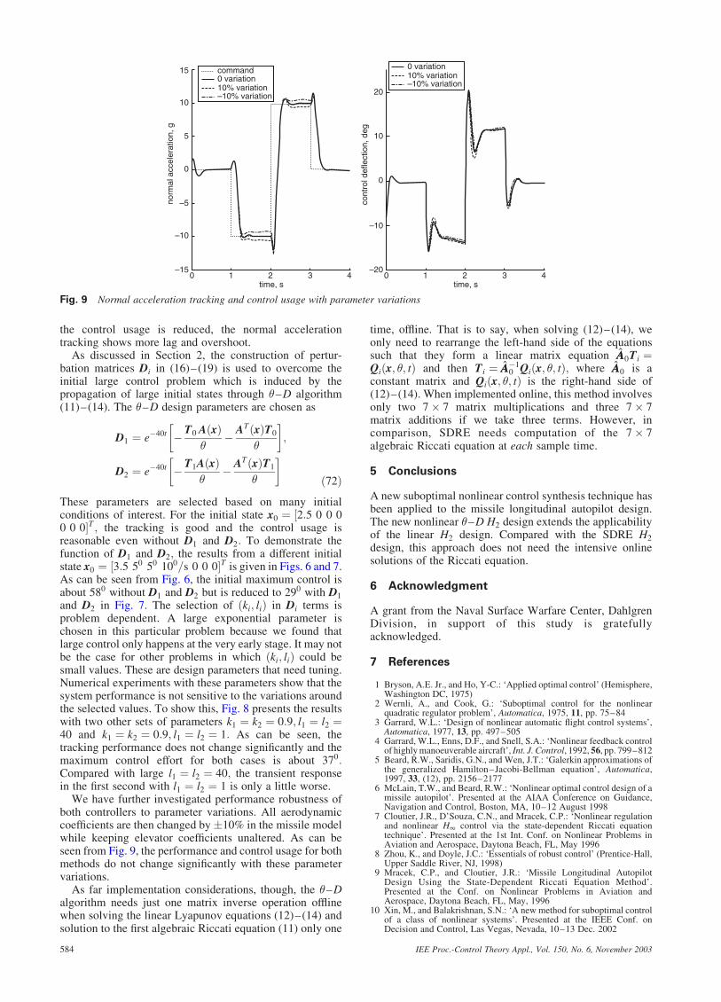
We have further investigated performance robustness ofboth controllers to parameter variations. All aerodynamiccoefficients are then changed by �10% in the missile modelwhile keeping elevator coefficients unaltered. As can beseen from Fig. 9, the performance and control usage for bothmethods do not change significantly with these parametervariations.
As far implementation considerations, though, the �–Dalgorithm needs just one matrix inverse operation offlinewhen solving the linear Lyapunov equations (12)–(14) andsolution to the first algebraic Riccati equation (11) only one
time, offline. That is to say, when solving (12)–(14), weonly need to rearrange the left-hand side of the equationssuch that they form a linear matrix equation AA0Ti ¼Qiðx; �; tÞ and then Ti ¼ AA1
0 Qiðx; �; tÞ; where AA0 is aconstant matrix and Qiðx; �; tÞ is the right-hand side of(12)–(14). When implemented online, this method involvesonly two 7 7 matrix multiplications and three 7 7matrix additions if we take three terms. However, incomparison, SDRE needs computation of the 7 7algebraic Riccati equation at each sample time.
5 Conclusions
A new suboptimal nonlinear control synthesis technique hasbeen applied to the missile longitudinal autopilot design.The new nonlinear �–D H2 design extends the applicabilityof the linear H2 design. Compared with the SDRE H2
design, this approach does not need the intensive onlinesolutions of the Riccati equation.
6 Acknowledgment
A grant from the Naval Surface Warfare Center, DahlgrenDivision, in support of this study is gratefullyacknowledged.
7 References
1 Bryson, A.E. Jr., and Ho, Y-C.: ‘Applied optimal control’ (Hemisphere,Washington DC, 1975)
2 Wernli, A., and Cook, G.: ‘Suboptimal control for the nonlinearquadratic regulator problem’, Automatica, 1975, 11, pp. 75–84
3 Garrard, W.L.: ‘Design of nonlinear automatic flight control systems’,Automatica, 1977, 13, pp. 497–505
4 Garrard, W.L., Enns, D.F., and Snell, S.A.: ‘Nonlinear feedback controlof highly manoeuverable aircraft’, Int. J. Control, 1992, 56, pp. 799–812
5 Beard, R.W., Saridis, G.N., and Wen, J.T.: ‘Galerkin approximations ofthe generalized Hamilton–Jacobi-Bellman equation’, Automatica,1997, 33, (12), pp. 2156–2177
6 McLain, T.W., and Beard, R.W.: ‘Nonlinear optimal control design of amissile autopilot’. Presented at the AIAA Conference on Guidance,Navigation and Control, Boston, MA, 10–12 August 1998
7 Cloutier, J.R., D’Souza, C.N., and Mracek, C.P.: ‘Nonlinear regulationand nonlinear H1 control via the state-dependent Riccati equationtechnique’. Presented at the 1st Int. Conf. on Nonlinear Problems inAviation and Aerospace, Daytona Beach, FL, May 1996
8 Zhou, K., and Doyle, J.C.: ‘Essentials of robust control’ (Prentice-Hall,Upper Saddle River, NJ, 1998)
9 Mracek, C.P., and Cloutier, J.R.: ‘Missile Longitudinal AutopilotDesign Using the State-Dependent Riccati Equation Method’.Presented at the Conf. on Nonlinear Problems in Aviation andAerospace, Daytona Beach, FL, May, 1996
10 Xin, M., and Balakrishnan, S.N.: ‘A new method for suboptimal controlof a class of nonlinear systems’. Presented at the IEEE Conf. onDecision and Control, Las Vegas, Nevada, 10–13 Dec. 2002
0
norm
al a
ccel
erat
ion,
g
–15
–10
–5
0
5
10
command0 variation10% variation–10% variation
15
1 2 3 4time, s
0
cont
rol d
efle
ctio
n, d
eg
–20
–10
0
10
20
1 2 3 4time, s
0 variation10% variation–10% variation
Fig. 9 Normal acceleration tracking and control usage with parameter variations
IEE Proc.-Control Theory Appl., Vol. 150, No. 6, November 2003584
Top Related