1

Midpoint Routing algorithms for Delaunay Triangulations

Weisheng Si and Albert Y. ZomayaCentre for Distributed and High Performance Computing

School of Information Technologies

2

The real life meaning of this paper:

Lazy man: If I only aim to reach the midpoint towards the destination in each move, can I reach the destination finally?

God: Yes, if you move on the class of graphs called Delaunay triangulations.

Prologue

3

Outline Background knowledge Related work Our work

The Midpoint Routing algorithm and its generalization

The Compass Midpoint algorithm and its generalization

Evaluation Open problem and Conclusion

4

Background Knowledge

Online routing

Our evaluation metrics for online routing

Delaunay triangulations

5

Online Routing In some networking scenarios, a packet only has

local information to find out its routes. Routing algorithms designed for such scenarios are called online routing algorithms.

We consider online routing in the same settings as those described in “Online routing in triangulations”: The environment is modeled by a geometric graph G(V, E),

where V is the set of nodes with known (x, y) coordinates and E is the set of links connecting the nodes.

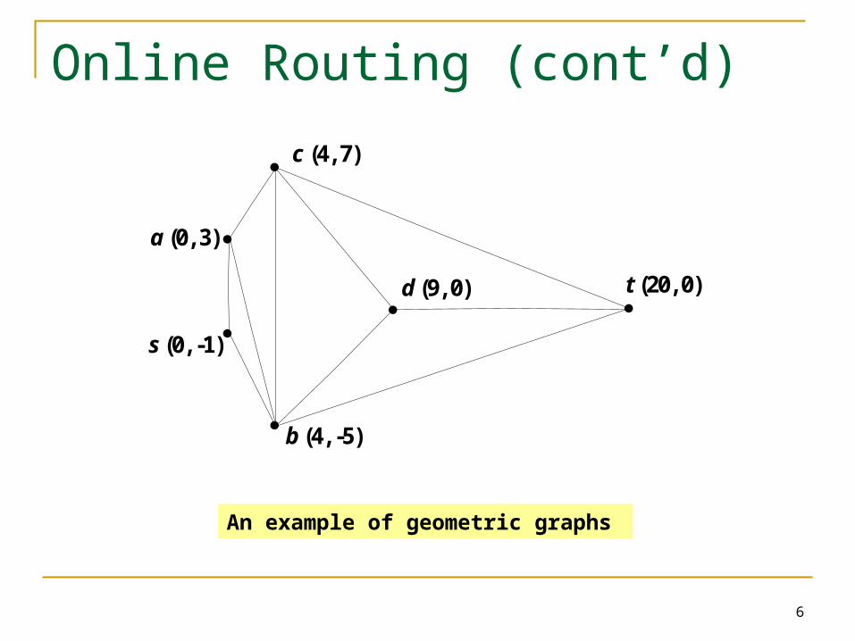
When a packet travels from a source node s to a destination node t, it carries the coordinates of t, and at each node v being visited, can learn the coordinates of the nodes in N(v), where N(v) denotes the set of v’s one-hop neighbors.

6

Online Routing (cont’d)

t (20, 0)

c (4, 7)

b (4, -5)

a (0, 3)

s (0, -1)

d (9, 0)

An example of geometric graphs

7

Online routing (cont’d) If an online routing algorithm A can move a packet

from any source s to any destination t in G, A is said to work for G.

If at each node v visited by a packet, A makes the routing decision for this packet only according to the coordinates of v, t, and the nodes in N(v), A is said to be memoryless or oblivious. ‘memoryless’ means that a packet records no information

learned during the traversal of a graph. Because the memoryless online routing (MOR) algorithms

have low complexity in both space and time for nodes and packets, they have received wide attention.

8

Our evaluation metrics for online routing For a source/destination pair (s, t) in G, we define

the deviation ratio of (s, t) by a routing algorithm A as the length of the path found by A from s to t versus the length of the shortest path from s to t.

For a graph G, we define the deviation ratio of G by A as the average deviation ratio of all (s, t) pairs in G.

In practice, the path length generally has two metrics: link distance link deviation ratio Euclidean distance Euclidean deviation ratio

9

Our evaluation metrics (cont’d) The deviation ratio concept is different from the c-

competitive concept A routing algorithm is c-competitive for a graph G, if for all

(s, t) pairs in G, their deviation ratios are not greater than a constant c.

The deviation ratio concept concerns the average performance of a routing algorithm on a graph, while the c-competitive concept concerns the worst-case performance of a routing algorithm on a graph.

The deviation ratio concept is different from the dilation concept and the stretch factor concept Both of them are defined to measure the path quality of a

subgraph with respect to the complete graph. Both of them are not used to evaluate routing algorithms.

10

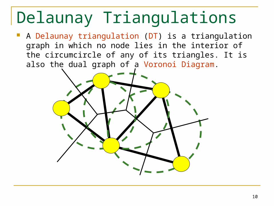
Delaunay Triangulations A Delaunay triangulation (DT) is a triangulation graph in

which no node lies in the interior of the circumcircle of any of its triangles. It is also the dual graph of a Voronoi Diagram.

11

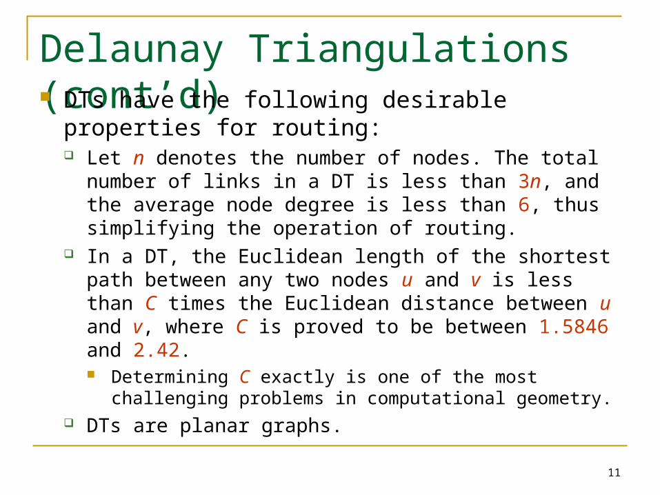
Delaunay Triangulations (cont’d) DTs have the following desirable properties for

routing: Let n denotes the number of nodes. The total number of

links in a DT is less than 3n, and the average node degree is less than 6, thus simplifying the operation of routing.

In a DT, the Euclidean length of the shortest path between any two nodes u and v is less than C times the Euclidean distance between u and v, where C is proved to be between 1.5846 and 2.42. Determining C exactly is one of the most challenging

problems in computational geometry. DTs are planar graphs.

12

Delaunay Triangulations (cont’d) Therefore, DTs have been widely proposed

as the network topologies.

In light of the above, this paper particularly focuses on the MOR algorithms for DTs.

13

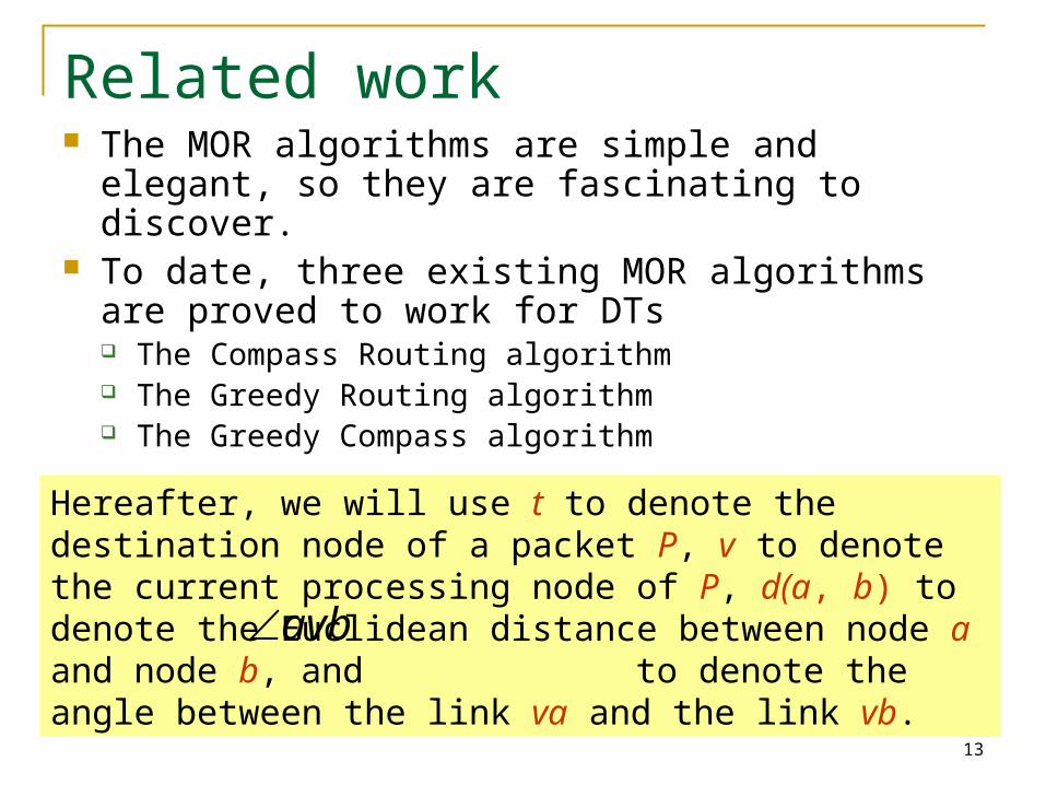
Related work The MOR algorithms are simple and elegant, so

they are fascinating to discover. To date, three existing MOR algorithms are proved

to work for DTs The Compass Routing algorithm The Greedy Routing algorithm The Greedy Compass algorithm

Hereafter, we will use t to denote the destination node of a packet P, v to denote the current processing node of P, d(a, b) to denote the Euclidean distance between node a and node b, and to denote the angle between the link va and the link vb.

avb

14

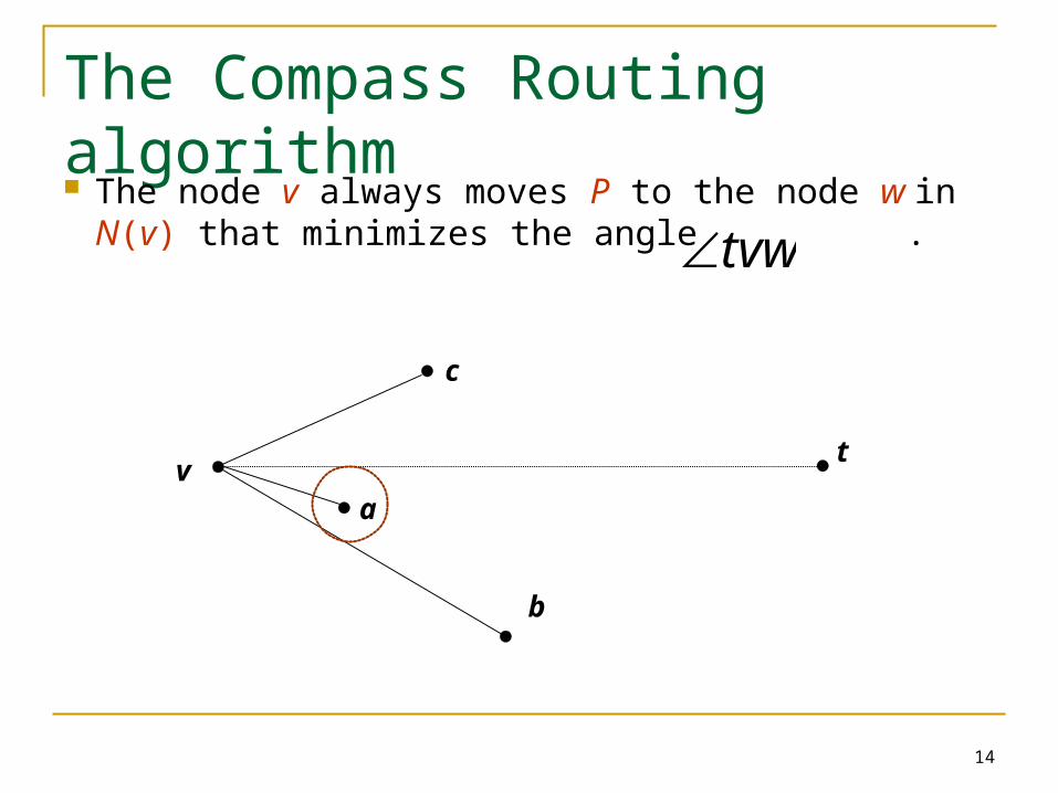
The Compass Routing algorithm The node v always moves P to the node w in

N(v) that minimizes the angle . tvw

v

c

t

b

a

15

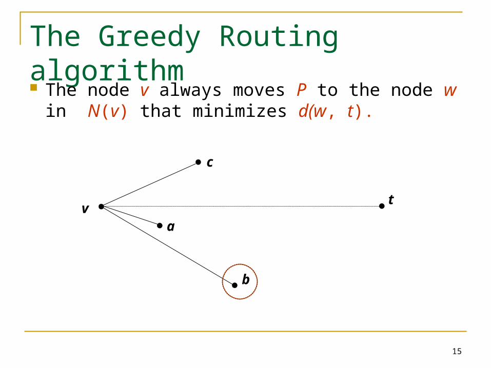
The Greedy Routing algorithm The node v always moves P to the node w in

N(v) that minimizes d(w, t).

v

c

t

b

a

16

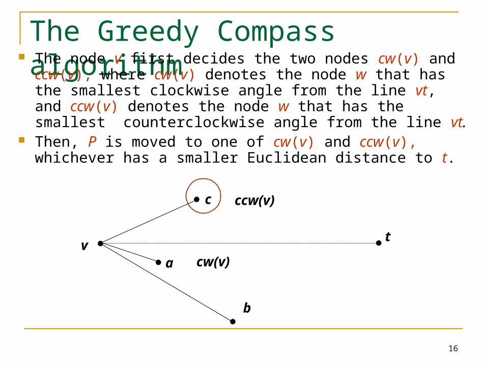
The Greedy Compass algorithm The node v first decides the two nodes cw(v) and ccw(v), where cw(v) denotes the node w that has the smallest clockwise angle from the line vt, and ccw(v) denotes the node w that has the smallest counterclockwise angle from the line vt.

Then, P is moved to one of cw(v) and ccw(v), whichever has a smaller Euclidean distance to t.

v

c

t

b

a

ccw(v)

cw(v)

17

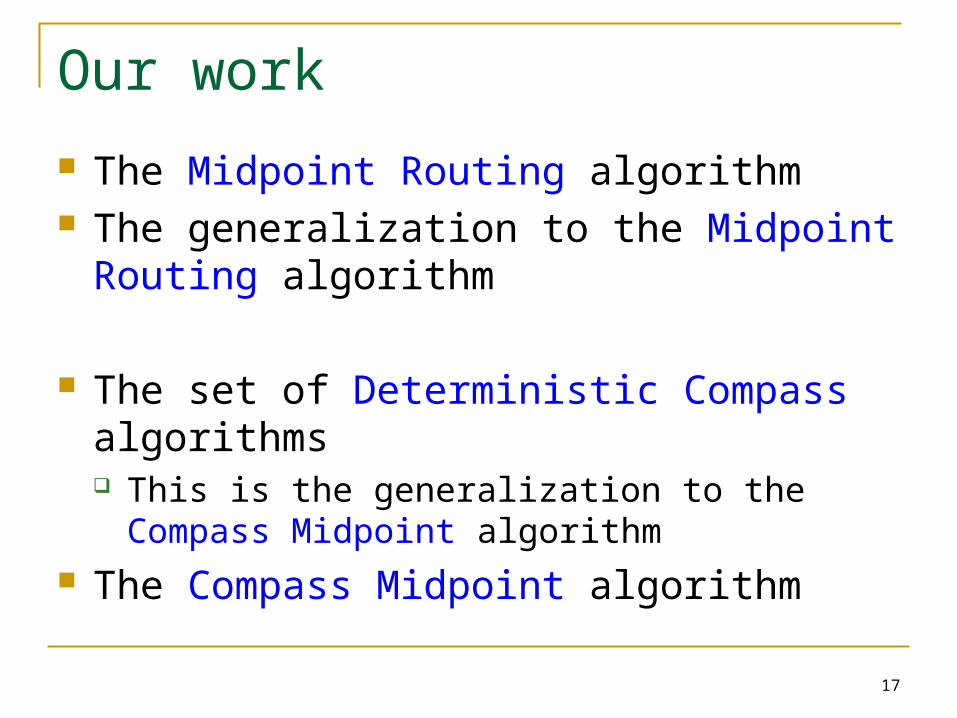
Our work

The Midpoint Routing algorithm The generalization to the Midpoint Routing

algorithm

The set of Deterministic Compass algorithms This is the generalization to the Compass

Midpoint algorithm The Compass Midpoint algorithm

18

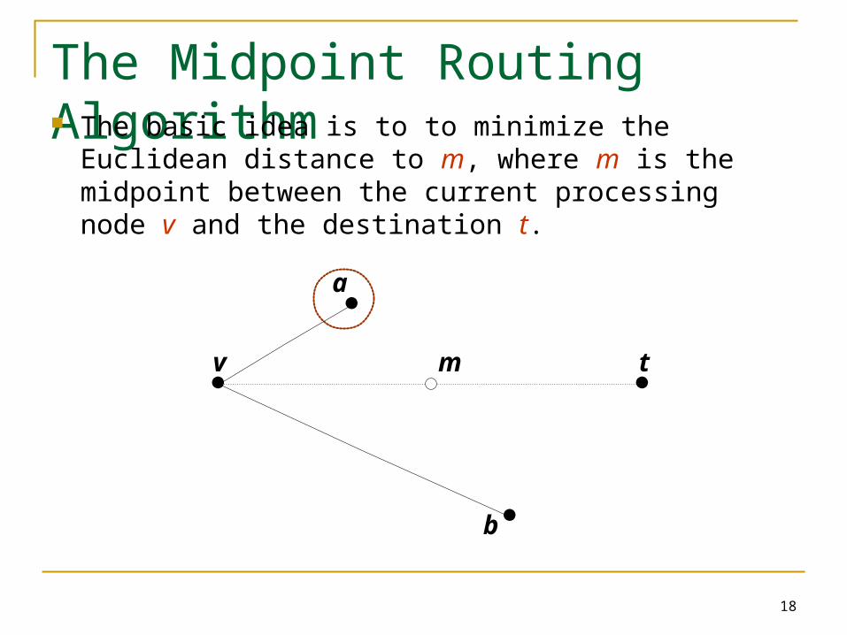
The Midpoint Routing Algorithm The basic idea is to to minimize the Euclidean

distance to m, where m is the midpoint between the current processing node v and the destination t.

tv

a

b

m

19

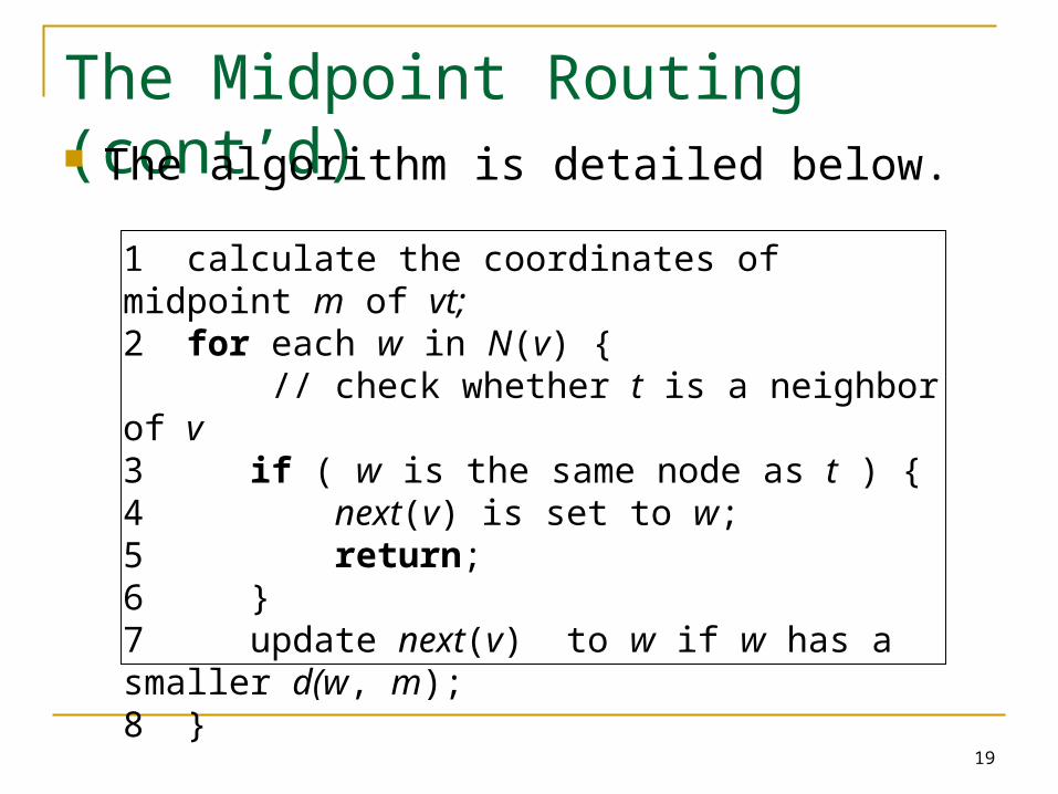
The Midpoint Routing (cont’d) The algorithm is detailed below.

1 calculate the coordinates of midpoint m of vt;2 for each w in N(v) { // check whether t is a neighbor of v3 if ( w is the same node as t ) {4 next(v) is set to w;5 return;6 }7 update next(v) to w if w has a smaller d(w, m);8 }

20

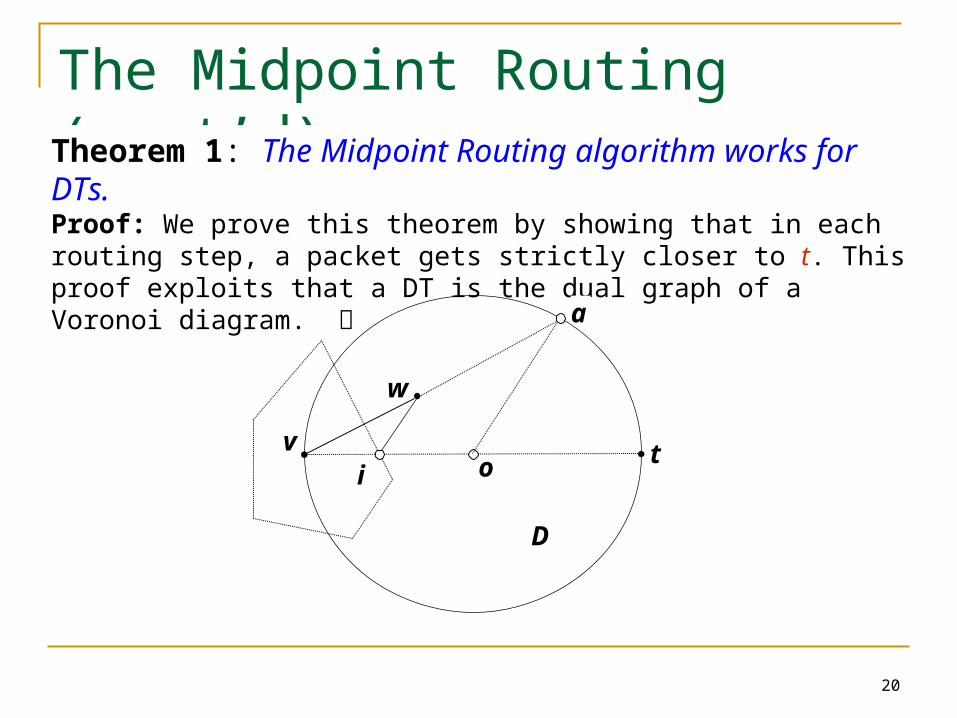
The Midpoint Routing (cont’d)Theorem 1: The Midpoint Routing algorithm works for DTs.Proof: We prove this theorem by showing that in each routing step, a packet gets strictly closer to t. This proof exploits that a DT is the dual graph of a Voronoi diagram.

ov

w

ti

D

a

21

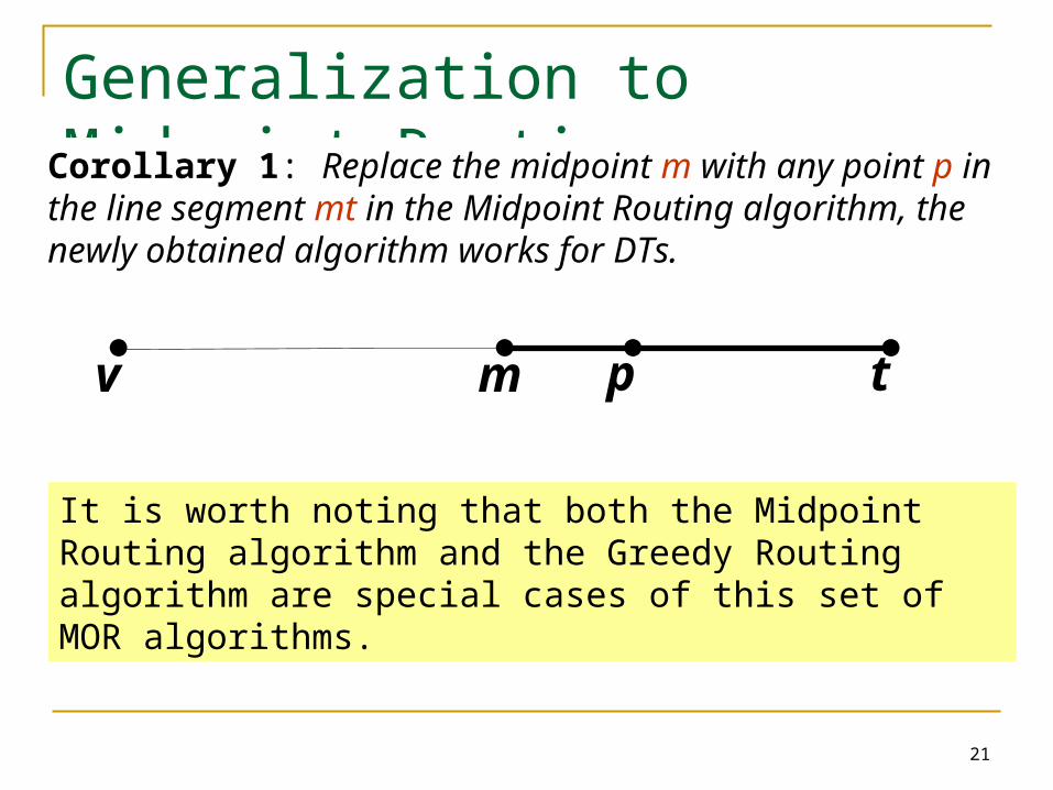
Generalization to Midpoint RoutingCorollary 1: Replace the midpoint m with any point p in the

line segment mt in the Midpoint Routing algorithm, the newly obtained algorithm works for DTs.

v tm p

It is worth noting that both the Midpoint Routing algorithm and the Greedy Routing algorithm are special cases of this set of MOR algorithms.

22

Generalization -- Proof

m

v

w

tp

Dm Dp

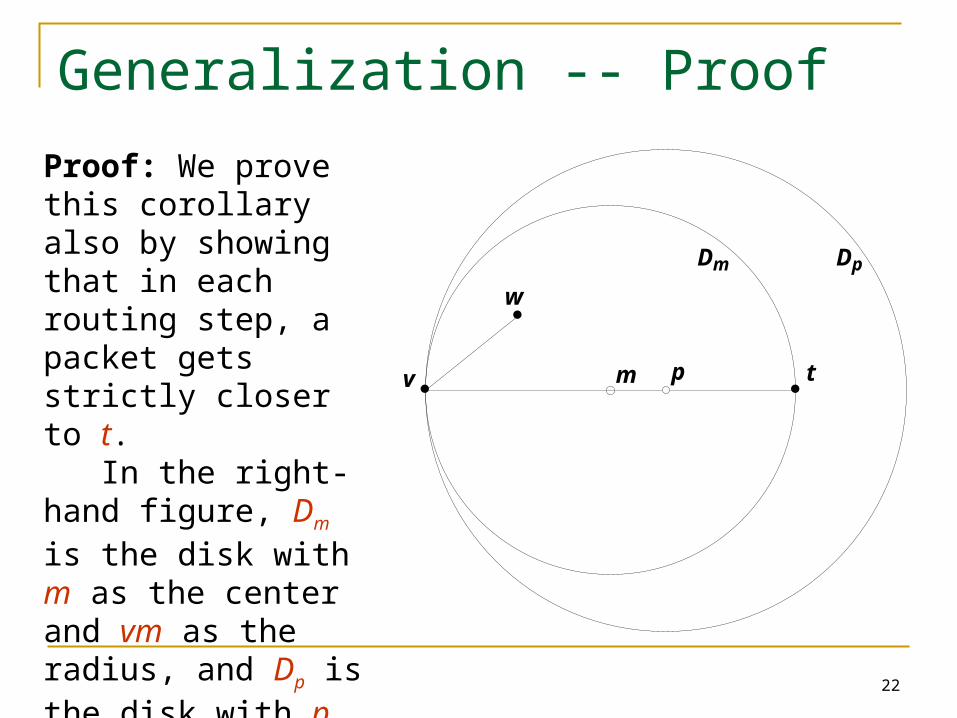
Proof: We prove this corollary also by showing that in each routing step, a packet gets strictly closer to t. In the right-hand figure, Dm is the disk with m as the center and vm as the radius, and Dp is the disk with p as the center and vp as the radius.

23

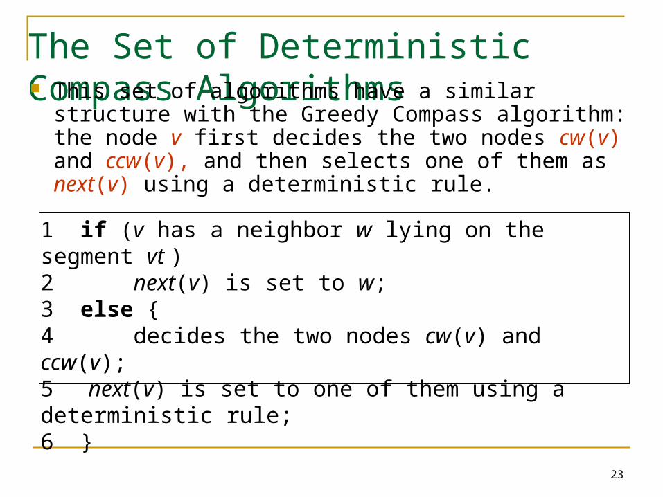
The Set of Deterministic Compass Algorithms This set of algorithms have a similar structure with the

Greedy Compass algorithm: the node v first decides the two nodes cw(v) and ccw(v), and then selects one of them as next(v) using a deterministic rule.

1 if (v has a neighbor w lying on the segment vt )2 next(v) is set to w; 3 else {4 decides the two nodes cw(v) and ccw(v);5 next(v) is set to one of them using a deterministic rule; 6 }

24

Proof Roadmap for “the set of Deterministic Compass algorithms work for DTs”

Lemma 1

Lemma 2

Theorem 2

Corollary 2

25

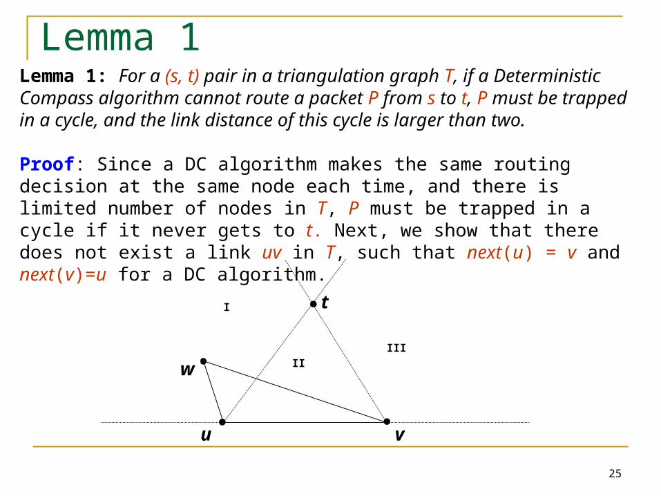
Lemma 1 Lemma 1: For a (s, t) pair in a triangulation graph T, if a Deterministic Compass algorithm cannot route a packet P from s to t, P must be trapped in a cycle, and the link distance of this cycle is larger than two.

Proof: Since a DC algorithm makes the same routing decision at the same node each time, and there is limited number of nodes in T, P must be trapped in a cycle if it never gets to t. Next, we show that there does not exist a link uv in T, such that next(u) = v and next(v)=u for a DC algorithm.

u

t

v

I

II

III

w

26

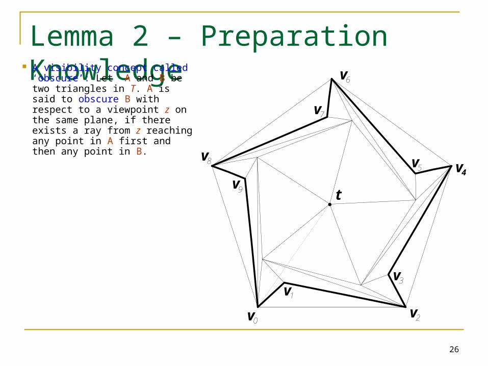
Lemma 2 – Preparation Knowledge A visibility concept called ‘obscure’: Let A and B be two triangles in T. A is said to obscure B with respect to a viewpoint z on the same plane, if there exists a ray from z reaching any point in A first and then any point in B.

t

v0

v1

v2

v3

v4v5

v6

v7

v8

v9

27

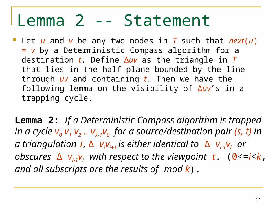
Lemma 2 -- Statement Let u and v be any two nodes in T such that next(u) = v

by a Deterministic Compass algorithm for a destination t. Define Δuv as the triangle in T that lies in the half-plane bounded by the line through uv and containing t. Then we have the following lemma on the visibility of Δuv’s in a trapping cycle.

Lemma 2: If a Deterministic Compass algorithm is trapped in a cycle v0 v1 v2… vk-1v0 for a source/destination pair (s, t) in a triangulation T, Δ vivi+1 is either identical to Δ vi-1vi or obscures Δ vi-1vi with respect to the viewpoint t. (0<=i<k, and all subscripts are the results of mod k).

28

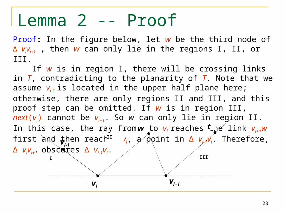
Lemma 2 -- ProofProof: In the figure below, let w be the third node of Δ vivi+1 , then w can only lie in the regions I, II, or III. If w is in region I, there will be crossing links in T, contradicting to the planarity of T. Note that we assume vi-1 is located in the upper half plane here; otherwise, there are only regions II and III, and this proof step can be omitted. If w is in region III, next(vi) cannot be vi+1. So w can only lie in region II. In this case, the ray from t to vi reaches the link vi+1w first and then reaches vi, a point in Δ vi-1vi. Therefore, Δ vivi+1 obscures Δ vi-1vi.

vi+1

I III

w t

vi-1

II

vi

29

Theorem 2 A triangulation is regular, if it can be obtained by

vertically projecting the faces of the lower convex hull of a 3-dimension polytope onto the plane.

Theorem 2: Any Deterministic Compass algorithm works for regular triangulations.

Proof: Edelsbrunner proved that if a triangulation T is a regular triangulation, T has no set of triangles that can form an obscuring cycle with respect to any viewpoint in T. Given Lemma 1 and Lemma 2, if a Deterministic Compass algorithm does not work for T, there must exist a set of triangles forming an obscuring cycle, thus causing contradictions. Therefore, this theorem holds.

30

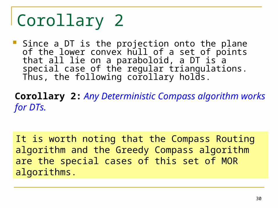
Corollary 2 Since a DT is the projection onto the plane of the lower

convex hull of a set of points that all lie on a paraboloid, a DT is a special case of the regular triangulations. Thus, the following corollary holds.

Corollary 2: Any Deterministic Compass algorithm works for DTs.

It is worth noting that the Compass Routing algorithm and the Greedy Compass algorithm are the special cases of this set of MOR algorithms.

31

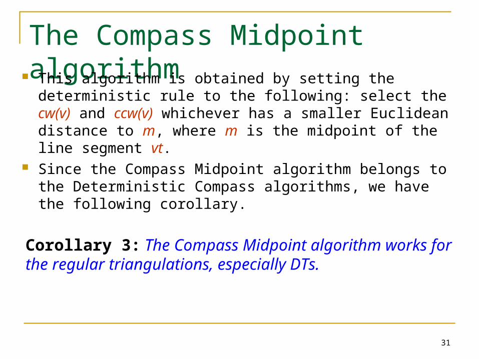
The Compass Midpoint algorithm This algorithm is obtained by setting the deterministic rule

to the following: select the cw(v) and ccw(v) whichever has a smaller Euclidean distance to m, where m is the midpoint of the line segment vt.

Since the Compass Midpoint algorithm belongs to the Deterministic Compass algorithms, we have the following corollary.

Corollary 3: The Compass Midpoint algorithm works for the regular triangulations, especially DTs.

32

Evaluations

Euclidean and link deviation ratios of the five MOR algorithms: Compass Routing Greedy Routing Greedy Compass Midpoint Routing Compass Midpoint

33

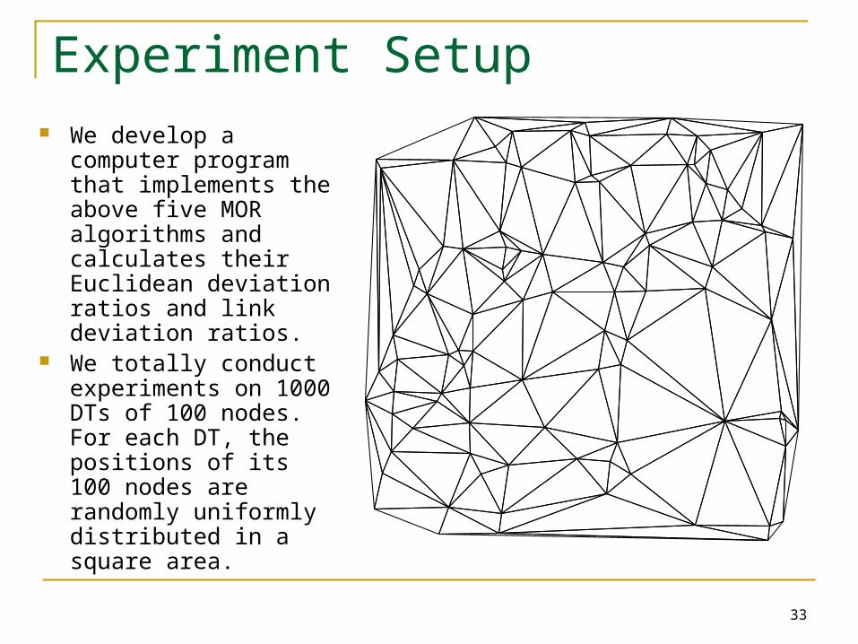
Experiment Setup We develop a computer

program that implements the above five MOR algorithms and calculates their Euclidean deviation ratios and link deviation ratios.

We totally conduct experiments on 1000 DTs of 100 nodes. For each DT, the positions of its 100 nodes are randomly uniformly distributed in a square area.

34

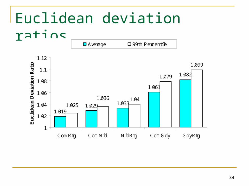
Euclidean deviation ratios

1.0191.029 1.033

1.061

1.082

1.04

1.079

1.099

1.0251.036

1

1.02

1.04

1.06

1.08

1.1

1.12

ComRtg ComMid MidRtg ComGdy GdyRtg

Eu

clid

ean

Dev

iati

on

Rat

io

Average 99th Percentile

35

Euclidean deviation ratios (cont’d) Both average and 99th percentile Euclidean deviation ratios

of these five algorithms are very small (all below 1.1). So all of them perform well in average and general cases, and

hence are practical for applications.

ComRtg performs the best, and the next four ones are in turn ComMid, MidRtg, ComGdy, and GdyRtg. This reflects that minimizing the angle to the destination at each

routing step is very effective in reducing the Euclidean distances of the paths, while minimizing the Euclidean distance to the destination is less effective.

The two new algorithms MidRtg and ComMid perform in the middle among these five algorithms.

36

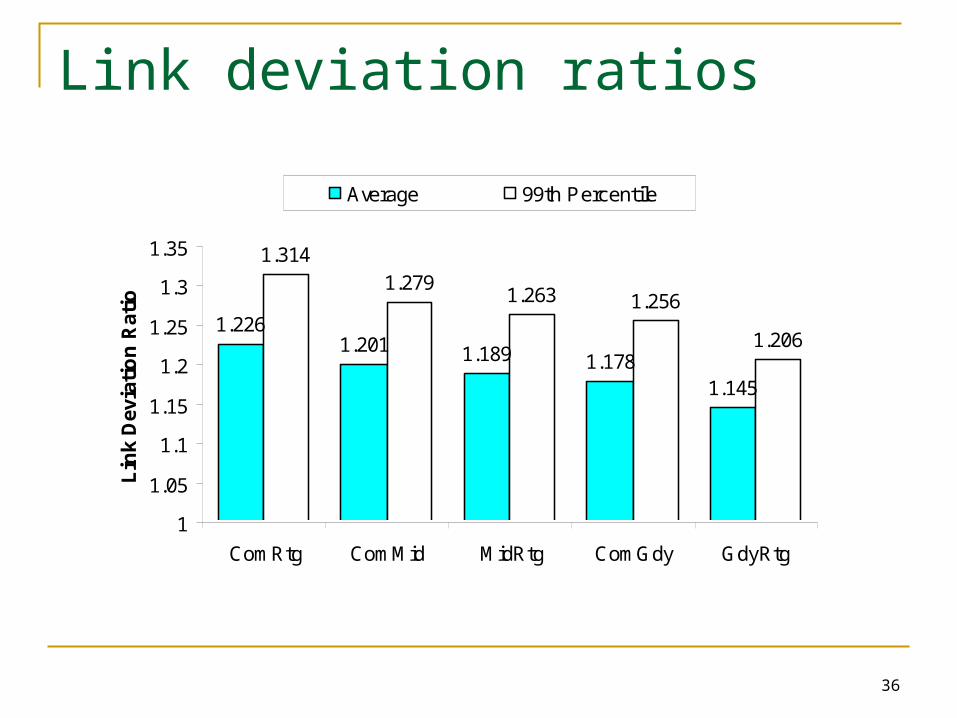
Link deviation ratios

1.2261.201 1.189 1.178

1.145

1.3141.279

1.263 1.256

1.206

1

1.05

1.1

1.15

1.2

1.25

1.3

1.35

ComRtg ComMid MidRtg ComGdy GdyRtg

Lin

k D

evia

tio

n R

atio

Average 99th Percentile

37

Link deviation ratios (cont’d) Both average and 99th percentile link deviation ratios of

these five algorithms are very small (all below 1.32). So all of them perform well in average and general cases, and

hence are practical for applications.

GdyRtg performs the best, and the next four ones are in turn ComGdy, MidRtg, ComMid, and ComRtg. This reflects that minimizing the Euclidean distance to the

destination at each routing step is very effective in reducing the link distances of the paths, while minimizing the angle to the destination is less effective.

The two new algorithms MidRtg and ComMid perform in the middle among these five algorithms.

38

An Open Problem It was proved that the Greedy Compass algorithm

works for arbitrary triangulations. Suggesting that combining the references to angles and

to Euclidean distances can generate more capable MOR algorithms.

This leads to the conjecture that the Compass Midpoint algorithm presented in this paper works for arbitrary triangulations.

Right now, we cannot prove or disprove this conjecture. If this conjecture is proved true, the Compass Midpoint algorithm becomes more meaningful.

39

Conclusions We found and proved two new MOR algorithms and two

new sets of MOR algorithms working for DTs. Our evaluations showed that

All the evaluated five algorithms can find paths with low link and Euclidean deviation ratios on DTs in average and general cases, so they are practical for applications.

The two algorithms perform in the middle among these five algorithms in terms of both link and Euclidean deviation ratios, so they are suitable for the applications requiring satisfactory performance in both link and Euclidean metrics.

Though our algorithms and proofs are simple, they possess an elementary nature, so they help in gaining insight into the MOR algorithms and the DTs.

40

Thank you!Questions and suggestions?