


Languages
Pages
Legal


Microneedle Mediated Transdermal
Vaccine Delivery
Aaron Tan, Michael Young, Samir Saidi, Chris Plunkett
October 29 2016
BENG 221

2
Table of Contents
Introduction 3
Problem Statement 4
Poke and Flow 4
Assumptions 4
Model Parameters 5
Analytical Solution 5
Numerical Solution 9
Poke and Patch 11
Model Parameters 11
Numerical Solution 11
Discussion and Conclusion 12
References 14
Appendix 15
MATLAB: Poke and Flow Analytical 15
MATLAB: Poke and Flow Numerical 16
MATLAB: Poke and Patch 18

3
Introduction
Vaccination remains one of the most
effective means of preventative medicine in
existence. A wide variety of viral diseases
ranging from flu strains to HPV have been
severely reduced in prevalence by vaccination
practices. Traditionally, these agents are
delivered via hypodermic needle or through
an aerosolized nasal spray providing an
efficient and rapid means of inoculation.
However, new and evolving methods geared
toward reducing total dosage, reducing
hazardous sharp wastes, and improving
effectiveness of the elicited immune response
continue to emerge. Among these novel
vaccination strategies is transdermal
administration. Vaccines show improved performance when delivered via transdermal administration due
to a large number of specialized “Langerhans” immune cells within the epidermal and dermal layers.
Figure 1 outlines the dermal layers and these specialized cells. Transdermal delivery also has the
advantage of circumventing first pass metabolism by the gastrointestinal tract and the liver thereby
maximizing cellular exposure to the antigen and immune response [1].
A large body of recent work in transdermal drug delivery has focused on microneedles. These devices
utilize an array of needles whose length and diameter are on the order of microns. Needles are able to
penetrate the stratum corneum and
expose epidermal tissue to the drug
payload while minimizing pain due to lack
of nerve endings. Furthermore, these
devices are small, manageable, and
sometimes degradable allowing for
improved handling administration and
medical waste. These traits have made
microneedle injection a promising mode
for vaccine delivery [2].
There are various methods for drug
delivery when utilizing microneedles.
Needles may be solid or hollow and are in
some cases degradable over time. Figure 2
illustrates four common strategies for
microneedle drug delivery. Poke and
Flow utilizes a hollow needle to inject a
small payload of agent into the epidermis
where it is then able to diffuse into the
Figure 1: Diagram of skin. Points of interest include
protective stratum corneum (15-20 um) that needs to be
bypassed for drug delivery, and the dermal (2000 um) and
epidermal (130-180 um) [1] layers that include immune
cells.
Figure 2: Drug is eluted through needles in poke-flow approach. In
poke-release, the needles are degradable and contain the drug. In
coat-poke, the drug is applied on the needles prior to penetration.
The poke-patch method uses micro-needles to create pores in the
skin; afterwards, a patch is placed on top of the penetration site. [3]
4
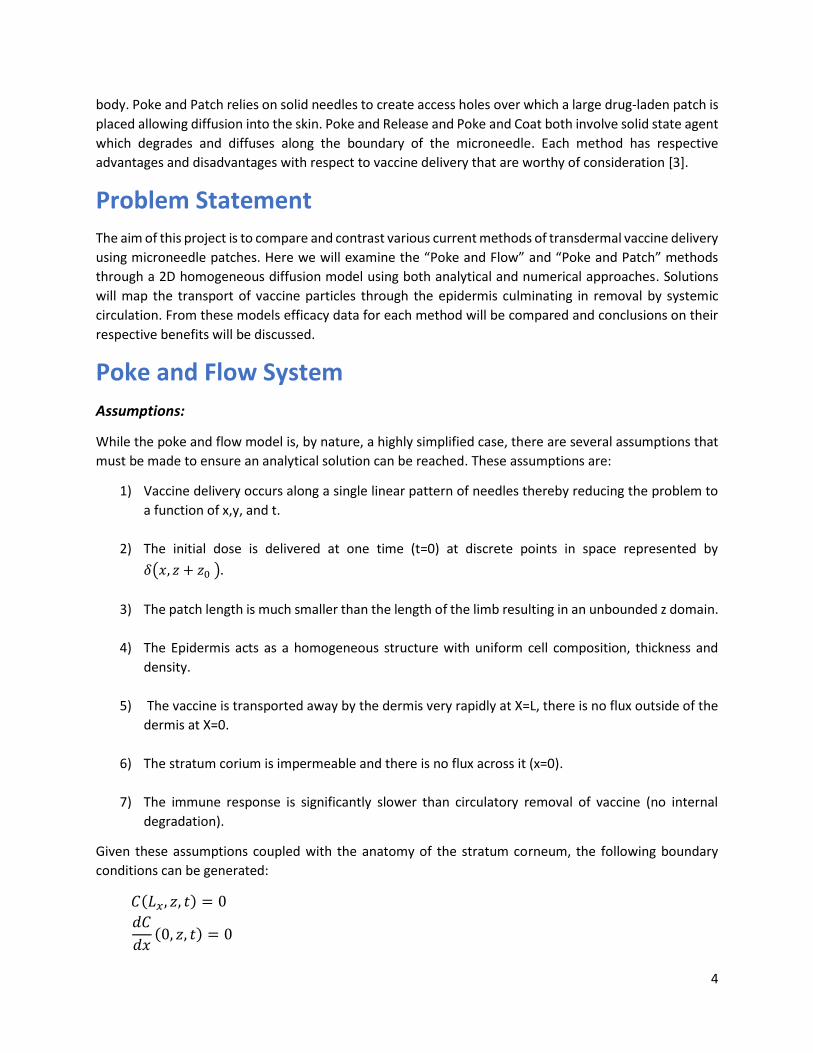
body. Poke and Patch relies on solid needles to create access holes over which a large drug-laden patch is
placed allowing diffusion into the skin. Poke and Release and Poke and Coat both involve solid state agent
which degrades and diffuses along the boundary of the microneedle. Each method has respective
advantages and disadvantages with respect to vaccine delivery that are worthy of consideration [3].
Problem Statement
The aim of this project is to compare and contrast various current methods of transdermal vaccine delivery
using microneedle patches. Here we will examine the “Poke and Flow” and “Poke and Patch” methods
through a 2D homogeneous diffusion model using both analytical and numerical approaches. Solutions
will map the transport of vaccine particles through the epidermis culminating in removal by systemic
circulation. From these models efficacy data for each method will be compared and conclusions on their
respective benefits will be discussed.
Poke and Flow System
Assumptions:
While the poke and flow model is, by nature, a highly simplified case, there are several assumptions that
must be made to ensure an analytical solution can be reached. These assumptions are:
1) Vaccine delivery occurs along a single linear pattern of needles thereby reducing the problem to
a function of x,y, and t.
2) The initial dose is delivered at one time (t=0) at discrete points in space represented by
𝛿(𝑥, 𝑧 + 𝑧0 ).
3) The patch length is much smaller than the length of the limb resulting in an unbounded z domain.
4) The Epidermis acts as a homogeneous structure with uniform cell composition, thickness and
density.
5) The vaccine is transported away by the dermis very rapidly at X=L, there is no flux outside of the
dermis at X=0.
6) The stratum corium is impermeable and there is no flux across it (x=0).
7) The immune response is significantly slower than circulatory removal of vaccine (no internal
degradation).
Given these assumptions coupled with the anatomy of the stratum corneum, the following boundary
conditions can be generated:
𝐶(𝐿𝑥, 𝑧, 𝑡) = 0
𝑑𝐶
𝑑𝑥(0, 𝑧, 𝑡) = 0

5
Z axis is unbounded (infinite)
As well as the following initial condition:
𝐶(𝑥, 𝑧, 0) = 𝐶0(𝛿 (𝑥, 𝑧 +𝐿𝑧
2) + 𝛿(𝑥, 𝑧 ) + 𝛿 (𝑥, 𝑧 −
𝐿𝑧
2))
Model Parameters:
The poke and flow model relies on
several experimentally or clinically
derived parameters. The first of these is
the initial vaccine antigen concentration
denoted as C0. Data derived from Fluvax,
an inactivated flu vaccine, set the antigen
dose at 10−10 𝜇𝑔/𝜇𝑚3 [4]. The second
major coefficient is the depth, Lx, of the
epidermis over which we wish to observe
diffusion. As shown in Figure XX, the
epidermis is a relatively thin layer and is
estimated here to be 75um across all z
(see assumption 4). While the limb itself
is unbounded in Z, the specific points of
the microneedles require a reference length
Lz. Here we hope to model 3 individual
microneedles and, by estimating needle
density in a recent study of transdermal
vaccination, a value of 500um was selected [1]. Finally, the diffusion constant of the epidermis must be
estimated for small molecules. This was done experimentally by Römgens et al. who employed
Fluorescence recovery after photo bleaching (FRAP) assay for molecules within the skin layers. By
observing migration of fluorescent molecules into the bleached region, a value of roughly9 𝜇𝑚2/𝑠 [6].
Given these coefficients we may proceed to an analytical solution for the model.
Analytical Solution:
The diffusion profile of the poke and flow approach was solved analytically, using a Green’s function. The
two-dimensional diffusion equation is shown, along with our initial condition of three separate
microneedle injections modeled by Dirac Delta functions and our homogeneous boundary conditions
(zero value at 𝑥 = 0, zero flux at 𝑥 = 𝐿𝑥, and unbounded in z). The x axis represents the depth into the
skin, and the z axis represents the length of the limb, which is assumed to be an infinite domain because
it is much longer than the thickness of the skin
Figure 3: H&E histology stain of skin with microneedle
injection sites. This figure demonstrates the orientation and
layers relevant to our 2D model showing X and Z directions as
well as the three needle locations [5].

6
Two-dimensional diffusion equation:
𝜕𝐶
𝜕𝑡= 𝐷 (
𝜕2𝐶
𝜕𝑥2+
𝜕2𝐶
𝜕𝑧2 )
Initial Condition:
𝐶(𝑥, 𝑧, 0) = 𝐶0 (𝛿 (𝑥, 𝑧 +𝐿𝑧
2) + 𝛿(𝑥, 𝑧) + 𝛿 (𝑥, 𝑧 −
𝐿𝑧
2))
Boundary Conditions: 𝜕
𝜕𝑥𝐶(0, 𝑧, 𝑡) = 0
𝐶(𝐿𝑥 , 𝑧, 𝑡) = 0
𝐶(𝑥, ±∞, 𝑡) = 0
The Green’s function for the problem is given by the product of the Green’s function in x and the Green’s
function in z (𝐺 = 𝑔𝑥𝑘 ∙ 𝑔𝑧𝑚). The full formulation is shown below.
Two-dimensional Green’s Function:
𝐺(𝑥, 𝑧, 𝑡; 𝑥0, 𝑧0, 𝑡0) = ∑ ∑ 𝑔𝑥𝑘(𝑥, 𝑡; 𝑥0, 𝑡0) ∙ 𝑔𝑧𝑚(𝑧, 𝑡; 𝑧0, 𝑡0)
𝑚𝑘
where
𝑔𝑥𝑘(𝑥, 𝑡; 𝑥0, 𝑡0) = ∑2
𝐿𝑥cos (
𝑘𝜋𝑥0
2𝐿𝑥) ∙ cos (
𝑘𝜋𝑥
2𝐿𝑥)
∞
𝑘=𝑜𝑑𝑑
𝑒−𝐷(
𝑘𝜋2𝐿𝑥
)2
(𝑡−𝑡0)
𝑔𝑧𝑚(𝑧, 𝑡; 𝑧0, 𝑡0) =1
√4𝜋𝐷(𝑡 − 𝑡0)𝑒
−(𝑧−𝑧0)2
4𝐷(𝑡−𝑡0)
Because this problem has homogeneous boundary conditions and does not contain a generation
or consumption term, the solution can be found by integrating the product of the initial condition as a
function of x0 and z0 and the Green’s Function over the x0 and z0 domains.
7
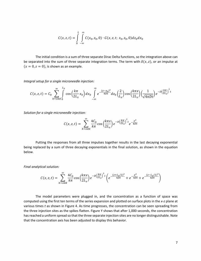
𝐶(𝑥, 𝑧, 𝑡) = ∫ ∫ 𝐶(𝑥0, 𝑧0, 0) ∙ 𝐺(𝑥, 𝑧, 𝑡; 𝑥0, 𝑧0, 0)𝑑𝑧0𝑑𝑥0
∞
−∞
𝐿
0
The initial condition is a sum of three separate Dirac Delta functions, so the integration above can
be separated into the sum of three separate integration terms. The term with 𝛿(𝑥, 𝑧), or an impulse at
(𝑥 = 0, 𝑧 = 0), is shown as an example.
Integral setup for a single microneedle injection:
𝐶(𝑥, 𝑧, 𝑡) = 𝐶0 ∑ ∫ cos (𝑘𝜋
2𝐿𝑥𝑥0) 𝑑𝑥0
𝐿𝑥
0
∞
𝑘=𝑜𝑑𝑑
∫ 𝑒−(𝑧−𝑧0)2
4𝐷𝑡 𝑑𝑧0
∞
−∞
(2
𝐿𝑥) cos (
𝑘𝜋𝑥
2𝐿𝑥) (
1
√4𝜋𝐷𝑡) 𝑒
−𝐷(𝑘𝜋2𝐿𝑥
)2
𝑡
Solution for a single microneedle injection:
𝐶(𝑥, 𝑧, 𝑡) = ∑4𝐶0
𝑘𝜋cos (
𝑘𝜋𝑥
2𝐿𝑥) 𝑒
−𝐷(𝑘𝜋2𝐿𝑥
)2
𝑡𝑒−
𝑧2
4𝐷𝑡
∞
𝑘=𝑜𝑑𝑑
Putting the responses from all three impulses together results in the last decaying exponential
being replaced by a sum of three decaying exponentials in the final solution, as shown in the equation
below.
Final analytical solution:
𝐶(𝑥, 𝑧, 𝑡) = ∑4𝐶0
𝑘𝜋cos (
𝑘𝜋𝑥
2𝐿𝑥) 𝑒
−𝐷(𝑘𝜋2𝐿𝑥
)2
𝑡(𝑒−
(𝑧+𝐿𝑧/2)2
4𝐷𝑡 + 𝑒−𝑧2
4𝐷𝑡 + 𝑒−(𝑧−𝐿𝑧/2)2
4𝐷𝑡 )
∞
𝑘=𝑜𝑑𝑑
The model parameters were plugged in, and the concentration as a function of space was
computed using the first ten terms of the series expansion and plotted on surface plots in the x-z plane at
various times t as shown in Figure 4. As time progresses, the concentration can be seen spreading from
the three injection sites as the spikes flatten. Figure Y shows that after 1,000 seconds, the concentration
has reached a uniform spread so that the three separate injection sites are no longer distinguishable. Note
that the concentration axis has been adjusted to display this behavior.

8
Figure 4: Concentration in the x-z plane at various times from 1 to 500 seconds.
Figure 5: Concentration in the x-z plane 1,000 seconds post-injection. Note that the concentration axis has
been adjusted to show the uniform concentration profile in the z direction, but the maximum concentration
is 2 orders of magnitude lower than the maximum concentration depicted by the spikes at t = 1 second.

9
Numerical Solution:
The numerical approximation to our problem was found by using finite differences. Finite
differences uses discrete substitutions for derivatives to find approximate values of the derivatives at each
point on a grid. First, the 2D space was discretized in the x and z directions into a grid with sizes ∆𝑥 and∆𝑧,
respectively. Time was discretized into units ∆𝑡 large. Next, the discretized approximations of the
derivatives could be used. They use points surrounding the point of interest in the spatial dimensions to
solve for the next point in time. The approximations are shown below.
𝜕𝐶
𝜕𝑡 →
𝐶(𝑥, 𝑧, 𝑡 + ∆𝑡) − 𝐶(𝑥, 𝑧, 𝑡)
∆𝑡
𝜕2𝐶
𝜕𝑥2 →
𝐶(𝑥 − ∆𝑥, 𝑧, 𝑡) − 2𝐶(𝑥, 𝑧, 𝑡) + 𝐶(𝑥 + ∆𝑥, 𝑧, 𝑡)
∆𝑥2
𝜕2𝐶
𝜕𝑧2 →
𝐶(𝑥, 𝑧 − ∆𝑧, 𝑡) − 2𝐶(𝑥, 𝑧, 𝑡) + 𝐶(𝑥, 𝑧 + ∆𝑧, 𝑡)
∆𝑧2
These can be substituted into the 2D diffusion equation to yield the following.
𝐶(𝑥, 𝑧, 𝑡 + ∆𝑡) − 𝐶(𝑥, 𝑧, 𝑡)
∆𝑡= 𝐷 (
𝐶(𝑥 − ∆𝑥, 𝑧, 𝑡) − 2𝐶(𝑥, 𝑧, 𝑡) + 𝐶(𝑥 + ∆𝑥, 𝑧, 𝑡)
∆𝑥2+
𝐶(𝑥, 𝑧 − ∆𝑧, 𝑡) − 2𝐶(𝑥, 𝑧, 𝑡) + 𝐶(𝑥, 𝑧 + ∆𝑧, 𝑡)
∆𝑧2)
Solving for the point we are interested in calculating, the equation becomes:
𝐶(𝑥, 𝑧, 𝑡 + ∆𝑡) = 𝐷 (𝐶(𝑥 − ∆𝑥, 𝑧, 𝑡) − 2𝐶(𝑥, 𝑧, 𝑡) + 𝐶(𝑥 + ∆𝑥, 𝑧, 𝑡)
∆𝑥2+
𝐶(𝑥, 𝑧 − ∆𝑧, 𝑡) − 2𝐶(𝑥, 𝑧, 𝑡) + 𝐶(𝑥, 𝑧 + ∆𝑧, 𝑡)
∆𝑧2) ∆𝑡 + 𝐶(𝑥, 𝑧, 𝑡)
We developed a script in MATLAB that would use the finite differences approximation above to
solve for the concentration values in 2D over time, given initial concentration values for every point in the
discretized grid. To simulate the poke and flow method, every point in the grid was set to zero except the
points representing the microneedles, which were set to the concentration C0. These values were then
allowed to change according to the values around them. The poke and patch method was simulated with
the same initial conditions, but at every time point, the points representing the microneedles were set to
C0. This represents the constant concentration of the vaccine at each of these points in the poke and
patch method.
The numerical approximation showed nearly the same concentration profile and dynamics as the
analytical solution. However, the scaling does not agree well. We believe that this has something to do
with the delta function in the analytical solution, because there is no equivalent for this in the discrete
domain. Surface plots of the concentration are shown below.

10
Figure 6: Numerical solution for the Patch and Flow method. The concentration starts out relatively high
and very localized, as is expected from the initial conditions. The peaks spread out and flatten while
rounding off at the top. Eventually, a relatively even concentration in the z-direction develops near the
microneedles.

11
Poke and Patch System
Model Parameters:
The “Poke and Patch” model operates on, unless otherwise stated, the
same assumptions, coefficients, boundary conditions, and initial
conditions. The notable exception which differentiates this model is the
constant reservoir of drug available rather than the instantaneous dose.
As shown in Figure 7, this is due to the generation of open punctures in
the skin which are covered by a large patch reservoir. This is reflected in
the boundary conditions which now reflect this as follows:
𝐶(𝑥 = 0, 𝑧= {−𝐿
2𝑧, 0,
𝐿
2𝑧} , 𝑡)=C0
𝐶(𝐿𝑥, 𝑧, 𝑡) = 0
𝑑𝐶
𝑑𝑥(0, 𝑧≠ {−
𝐿
2𝑧, 0,
𝐿
2𝑧} , 𝑡) = 0
𝑑𝐶
𝑑𝑧(𝑥, −𝐿𝑧 , 𝑡) =
𝑑𝐶
𝑑𝑧(𝑥, 𝐿𝑧 , 𝑡) = 0
In order to evaluate a solution, the initial condition at time=0 is changed
to state that the concentration at all points in the model is 0 shown below
as:
𝐶(𝑥, 𝑧, 0) = 0
Numerical Solution:
The poke and patch model starts out identical to the poke and flow
method, but the models quickly become different. Instead of widening
and flattening the peaks, the peaks stay pinned at the C0 value while the
“valleys” in between the peaks become shallower and shallower. The
concentration values end up much higher overall, as is expected for a
continuous release of vaccine instead of the instantaneous release of
vaccine. Surface plots of the poke and patch model are shown below.
Figure 7: Poke and Patch
method graphical overview.
Holes are generated by a
solid needle and then covered
by a large patch containing a
relatively large concentration
of drug or antigen [7].

12
Discussion and Conclusion
The data modeled here suggests that the Poke and Patch method may produce superior results.
At 1,000 seconds post-injection, the minimum concentration of any point in the space enclosed by the
three needles is more than an order of magnitude higher in the Poke and Patch model than in the Poke
and Flow model. This means that a much greater overall dose can be achieved using the Poke and Patch
method. Additionally, Poke and Patch utilizes solid needles which are less prone to failure and are more
structurally sound. The inclusion of a patch also makes dose alterations much more manageable as
antigen flux can be stopped at any time [2].
Despite the observed advantages for Poke and Patch, there are several inherent limitations within
our model that may interfere with results. As stated above, there is a scaling discrepancy with the
numerical solution for the Poke and Flow model. While the root cause is unknown, it likely arise from the
use of 𝛿(𝑥, 𝑧) functions to describe dose points. Despite interest in the Poke and Release and Poke and
Figure 8: Numerical solution for the Poke and Patch method. Values begin at a high concentration at the
site of needle injection. Over time, valleys between peaks form and steadily increase suggesting
increased coverage.
13
Coat methods, our model is currently unable to resolve the complex boundary of a degrading needle.
Thus, for our methods, the injection site is compressed to a single point. For our Poke and Patch solution,
the issue of depletion is never fully addressed. In practice, the concentration of drug within the patch
would decrease as a function of time though our model assumes the reservoir is so large this is negligible.
Finally, it should be noted that the method of action by which vaccines operate is through the immune
response. The breakdown of vaccine and corresponding generation of antibodies and antigen presenting
cells is not modeled as an inhomogeneous sink term in this model.
Future attempts at microneedle delivery modeling will focus first on the immune response.
Obtaining a reliable value for in-vivo breakdown of antigen will likely require experimentation though,
with this data, the model can be vastly improved in accuracy. Following this improvements to boundary
value modeling aimed at incorporating the needle geometry will allow for studies of more advanced
methods of transdermal delivery such as Poke and Coat. Finally, expansion to a full 3D geometry of
needles would allow for modeling of complex patterns that may optimize dose coverage across the
epidermis. These areas of improvement serve as excellent ways to advance the model as well as our
understanding of transdermal delivery.

14
References
[1] Koen van der Maaden, Wim Jiskoot, Joke Bouwstra, Microneedle technologies for (trans)dermal drug
and vaccine delivery, Journal of Controlled Release, Volume 161, Issue 2, 20 July 2012, Pages
645-655, ISSN 0168-3659, http://dx.doi.org/10.1016/j.jconrel.2012.01.042.
[2] Kim Y-C, Park J-H, Prausnitz MR. Microneedles for drug and vaccine delivery. Advanced drug delivery
reviews. 2012;64(14):1547-68.
[3] Prausnitz MR, Langer R. Transdermal drug delivery. Nature biotechnology. 2008;26(11):1261-1268.
doi:10.1038/nbt.1504.
[4] Fluvax Data Sheet. CSL Biotherapies. 2016
[5] Sullivan, S.P. et al. Dissolving polymer microneedle patches for influenza vaccination. Nat Med 16,
915-920 (2010).
[6] Römgens, Anne M., et al. "Diffusion profile of macromolecules within and between human skin
layers for (trans) dermal drug delivery." Journal of the mechanical behavior of biomedical
materials 50 (2015): 215-222.
[7] Ita, Kevin. "Transdermal delivery of drugs with microneedles—Potential and
challenges." Pharmaceutics 7.3 (2015): 90-105.
15
Appendix
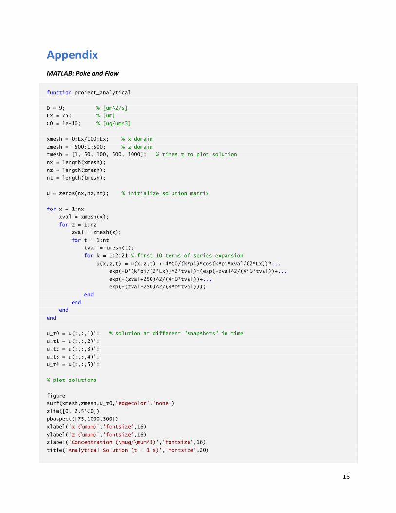
MATLAB: Poke and Flow
function project_analytical
D = 9; % [um^2/s]
Lx = 75; % [um]
C0 = 1e-10; % [ug/um^3]
xmesh = 0:Lx/100:Lx; % x domain
zmesh = -500:1:500; % z domain
tmesh = [1, 50, 100, 500, 1000]; % times t to plot solution
nx = length(xmesh);
nz = length(zmesh);
nt = length(tmesh);
u = zeros(nx,nz,nt); % initialize solution matrix
for x = 1:nx
xval = xmesh(x);
for z = 1:nz
zval = zmesh(z);
for t = 1:nt
tval = tmesh(t);
for k = 1:2:21 % first 10 terms of series expansion
u(x,z,t) = u(x,z,t) + 4*C0/(k*pi)*cos(k*pi*xval/(2*Lx))*...
exp(-D*(k*pi/(2*Lx))^2*tval)*(exp(-zval^2/(4*D*tval))+...
exp(-(zval+250)^2/(4*D*tval))+...
exp(-(zval-250)^2/(4*D*tval)));
end
end
end
end
u_t0 = u(:,:,1)'; % solution at different "snapshots" in time
u_t1 = u(:,:,2)';
u_t2 = u(:,:,3)';
u_t3 = u(:,:,4)';
u_t4 = u(:,:,5)';
% plot solutions
figure
surf(xmesh,zmesh,u_t0,'edgecolor','none')
zlim([0, 2.5*C0])
pbaspect([75,1000,500])
xlabel('x (\mum)','fontsize',16)
ylabel('z (\mum)','fontsize',16)
zlabel('Concentration (\mug/\mum^3)','fontsize',16)
title('Analytical Solution (t = 1 s)','fontsize',20)

16
figure
surf(xmesh,zmesh,u_t1,'edgecolor','none')
zlim([0, 2.5*C0])
pbaspect([75,1000,500])
xlabel('x (\mum)','fontsize',16)
ylabel('z (\mum)','fontsize',16)
zlabel('Concentration (\mug/\mum^3','fontsize',16)
title('Analytical Solution (t = 50 s)','fontsize',20)
figure
surf(xmesh,zmesh,u_t2,'edgecolor','none')
zlim([0, 2.5*C0])
pbaspect([75,1000,500])
xlabel('x (\mum)','fontsize',16)
ylabel('z (\mum)','fontsize',16)
zlabel('Concentration (\mug/\mum^3)','fontsize',16)
title('Analytical Solution (t = 100 s)','fontsize',20)
figure
surf(xmesh,zmesh,u_t3,'edgecolor','none')
zlim([0, 2.5*C0])
pbaspect([75,1000,500])
xlabel('x (\mum)','fontsize',16)
ylabel('z (\mum)','fontsize',16)
zlabel('Concentration (\mug/\mum^3)','fontsize',16)
title('Analytical Solution (t = 500 s)','fontsize',20)
figure
surf(xmesh,zmesh,u_t4,'edgecolor','none')
pbaspect([75,1000,500])
xlabel('x (\mum)','fontsize',16)
ylabel('z (\mum)','fontsize',16)
zlabel('Concentration (\mug/\mum^3)','fontsize',16)
title('Analytical Solution (t = 1000 s)','fontsize',20)
end
Published with MATLAB® R2015b
MATLAB: Poke and Flow
%%Program for making animation from array C
%Plot first frame
s = surf(z,x,C(:,:,1),'edgecolor','none');
%Set aspect ratio and axis for better viewing
pbaspect([750 75 750])
axis([0 1000 0 75 0 .02])
%Label figure

17
title('Numerical Solution (Finite Differences)')
xlabel('z (\mum)')
ylabel('x (\mum)')
zlabel('Concentration (\mug/\mum^3)*10^-^1^0')
%open video file
vidObj = VideoWriter('AnimationImp.avi');
open(vidObj);
% Step size (30 in this case) determines frame rate
for i = 1:30:length(C(1,1,:));
%updates data in the plot
s.ZData = C(:,:,i);
%captures frame
F = getframe(gcf);
%writes to video
writeVideo(vidObj,F);
end
%close video file
close(vidObj);
%Plots single figure at t = 1,50,100,200,500
figure
s = surf(z,x,C(:,:,10),'edgecolor','none');
title('Numerical Solution (t = 1 s)')
xlabel('z (\mum)')
ylabel('x (\mum)')
zlabel('Concentration (\mug/\mum^3)*10^-^1^0')
pbaspect([750 75 750])
axis([0 1000 0 75 0 .02])
figure
s = surf(z,x,C(:,:,500),'edgecolor','none');
title('Numerical Solution (t = 50 s)')
xlabel('z (\mum)')
ylabel('x (\mum)')
zlabel('Concentration (\mug/\mum^3)*10^-^1^0')
pbaspect([750 75 750])
axis([0 1000 0 75 0 .02])
figure
s = surf(z,x,C(:,:,1000),'edgecolor','none');
title('Numerical Solution (t = 100 s)')
xlabel('z (\mum)')
ylabel('x (\mum)')
zlabel('Concentration (\mug/\mum^3)*10^-^1^0')
pbaspect([750 75 750])
axis([0 1000 0 75 0 .02])
figure
s = surf(z,x,C(:,:,2000),'edgecolor','none');
title('Numerical Solution (t = 200 s)')
xlabel('z (\mum)')

18
ylabel('x (\mum)')
zlabel('Concentration (\mug/\mum^3)*10^-^1^0')
pbaspect([750 75 750])
axis([0 1000 0 75 0 .02])
figure
s = surf(z,x,C(:,:,5000),'edgecolor','none');
title('Numerical Solution (t = 500 s)')
xlabel('z (\mum)')
ylabel('x (\mum)')
zlabel('Concentration (\mug/\mum^3)*10^-^1^0')
pbaspect([750 75 750])
axis([0 1000 0 75 0 .02])
Published with MATLAB® R2015b
MATLAB: Poke and Patch
%%Program for making animation from array C
%Plot first frame
s = surf(z,x,C(:,:,1),'edgecolor','none');
%Set aspect ratio and axis for better viewing
pbaspect([750 75 750])
axis([0 1000 0 75 0 .02])
%Label figure
title('Numerical Solution (Finite Differences)')
xlabel('z (\mum)')
ylabel('x (\mum)')
zlabel('Concentration (\mug/\mum^3)*10^-^1^0')
%open video file
vidObj = VideoWriter('AnimationImp.avi');
open(vidObj);
% Step size (30 in this case) determines frame rate
for i = 1:30:length(C(1,1,:));
%updates data in the plot
s.ZData = C(:,:,i);
%captures frame
F = getframe(gcf);
%writes to video
writeVideo(vidObj,F);
end
%close video file
close(vidObj);

19
%Plots single figure at t = 1,50,100,200,500
figure
s = surf(z,x,C(:,:,10),'edgecolor','none');
title('Numerical Solution (t = 1 s)')
xlabel('z (\mum)')
ylabel('x (\mum)')
zlabel('Concentration (\mug/\mum^3)*10^-^1^0')
pbaspect([750 75 750])
axis([0 1000 0 75 0 .02])
figure
s = surf(z,x,C(:,:,500),'edgecolor','none');
title('Numerical Solution (t = 50 s)')
xlabel('z (\mum)')
ylabel('x (\mum)')
zlabel('Concentration (\mug/\mum^3)*10^-^1^0')
pbaspect([750 75 750])
axis([0 1000 0 75 0 .02])
figure
s = surf(z,x,C(:,:,1000),'edgecolor','none');
title('Numerical Solution (t = 100 s)')
xlabel('z (\mum)')
ylabel('x (\mum)')
zlabel('Concentration (\mug/\mum^3)*10^-^1^0')
pbaspect([750 75 750])
axis([0 1000 0 75 0 .02])
figure
s = surf(z,x,C(:,:,2000),'edgecolor','none');
title('Numerical Solution (t = 200 s)')
xlabel('z (\mum)')
ylabel('x (\mum)')
zlabel('Concentration (\mug/\mum^3)*10^-^1^0')
pbaspect([750 75 750])
axis([0 1000 0 75 0 .02])
figure
s = surf(z,x,C(:,:,5000),'edgecolor','none');
title('Numerical Solution (t = 500 s)')
xlabel('z (\mum)')
ylabel('x (\mum)')
zlabel('Concentration (\mug/\mum^3)*10^-^1^0')
pbaspect([750 75 750])
axis([0 1000 0 75 0 .02])
Published with MATLAB® R2015b
Top Related